

Submitted:
16 September 2026
Posted:
17 September 2026
You are already at the latest version
Abstract
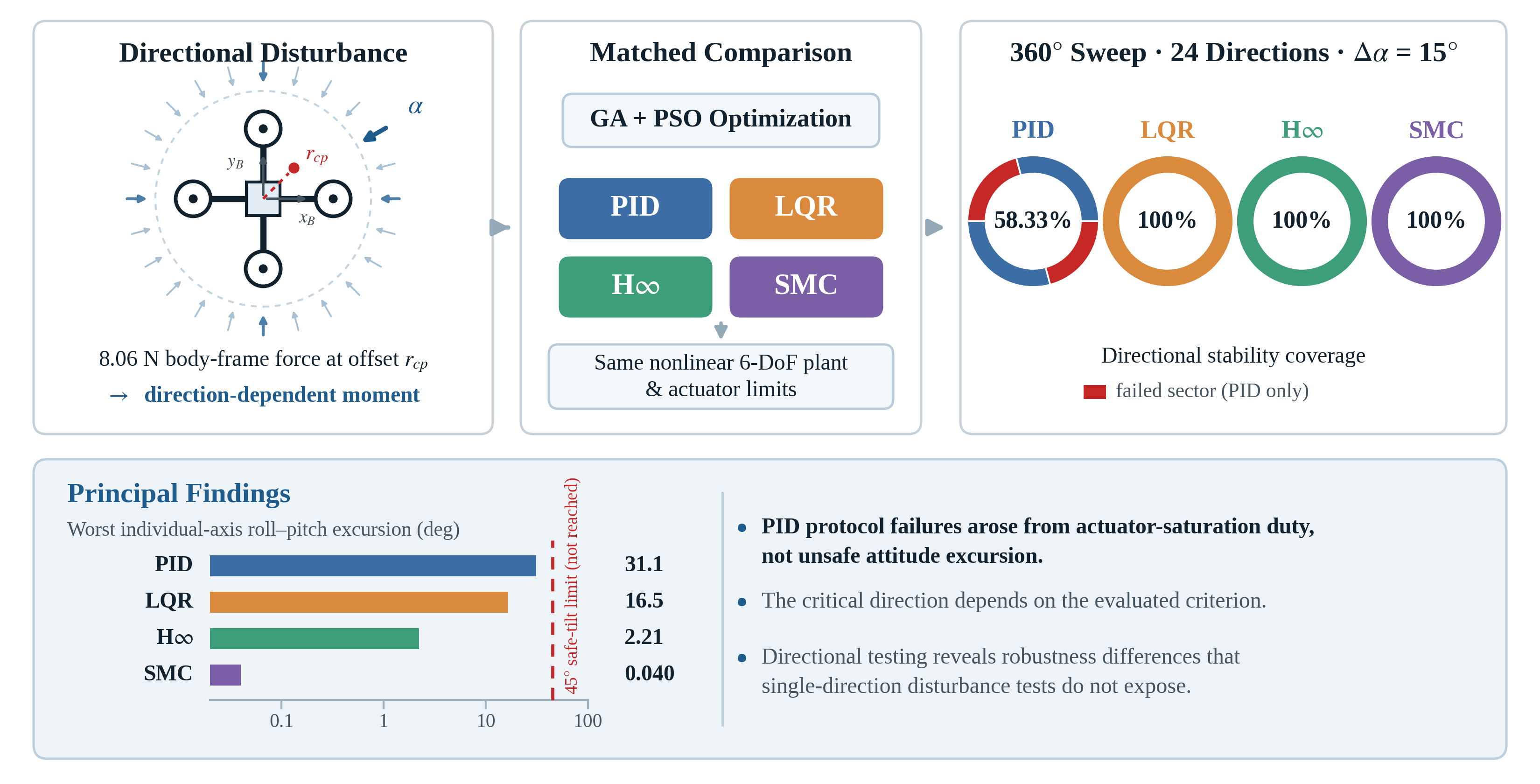
Quadrotor attitude controllers are usually evaluated against wind arriving from a single direction, leaving the directional structure of attitude robustness and actuator-limited failure poorly characterized. This study compares proportional–integral–derivative (PID), linear quadratic regulator (LQR), H-infinity and sliding mode controllers within a unified framework in which a real-coded genetic algorithm and particle swarm optimization tune every configuration against an identical objective, plant and constraint set. A nonlinear six-degree-of-freedom Newton–Euler model with actuator saturation supports three scenarios: step tracking under a finite-duration wind force, sustained helical tracking, and a complete 0 to 360 degree azimuthal sweep of a body-frame disturbance moment at 15 degree resolution. Sliding mode control achieved the best helical tracking accuracy, reducing position root-mean-square error from 1.079 to 0.677 metres, the smallest directional excursion of 0.040 degrees, and the lowest saturation duty of 9.2 percent; LQR required the lowest normalized control effort; and H-infinity combined near-circular directional envelopes with nearly immediate attitude recovery. PID retained stable directional coverage over only 58.33% of azimuths, failing solely through saturation duty above the adopted limit rather than unsafe tilt. Overall, SMC and H∞ maximize disturbance suppression, whereas LQR offers the best trade-off between tracking accuracy and control efficiency for autonomous flight in windy environments.
Keywords:
quadrotor UAV
; directional wind disturbance
; attitude robustness
; actuator saturation
; sliding mode control
; H-infinity control
; linear quadratic regulator
; post-disturbance recovery
1. Introduction
Quadrotor unmanned aerial vehicles (UAVs) are widely used in inspection, mapping, monitoring, transportation, and autonomous-flight research because of their vertical take-off and landing, hovering, and maneuverability. Their nonlinear, multivariable, underactuated, and open-loop unstable dynamics, however, strongly couple translational and rotational motion and make closed-loop performance sensitive to modeling uncertainty, aerodynamic loads, actuator limits, and external disturbances [1,2,3]. Consequently, meaningful controller assessment should extend beyond nominal hover and isolated step responses.
No single control architecture provides the best combination of tracking accuracy, robustness, control effort, and implementation complexity under all conditions. Comparative studies report different rankings depending on the plant, trajectory, constraints, and performance metrics [4,5,6]. Fair comparison therefore requires a common nonlinear plant, identical actuator limits and disturbance scenarios, and consistent evaluation criteria.
PID control remains attractive because of its simplicity and low computational cost, although its performance depends strongly on gain selection and operating conditions. Robust-adaptive and intelligent PID variants [7,8], as well as GA- and PSO-based tuning approaches [9,10], have therefore been investigated; PSO has also been combined with sliding-mode tuning and disturbance-observer compensation [11]. LQR provides systematic state-feedback design and has demonstrated effective quadrotor stabilization and trajectory tracking [4,12], but its linearized design requires validation on the nonlinear constrained plant. Robust formulations explicitly address disturbance attenuation and have been applied to cascaded quadrotor control and wind rejection [13,14].
SMC is particularly attractive for rejecting matched uncertainties and disturbances. Quadrotor studies include foundational backstepping and sliding-mode designs [15], fast-terminal manifolds [16], finite- and fixed-time disturbance observers [17,18], experimentally evaluated disturbance-observer SMC [19], dynamic sliding modes [20], adaptive integral-terminal designs [21], saturation-aware adaptive SMC [22], high-order disturbance observers [23], and super-twisting or finite-time formulations [24,25]. However, differences in models, constraints, objectives, and disturbance definitions make direct cross-study ranking of PID, LQR, , and SMC difficult.
Two comparative studies are especially relevant. Al-Qadasi et al. [26] compared GA- and PSO-tuned PID, LQR, and attitude controllers under nominal response, wind gusts, and actuator saturation, but excluded SMC, full six-degree-of-freedom trajectory tracking, and directional robustness analysis. Rinaldi et al. [6] compared PID, LQR, model predictive control, feedback linearization, and SMC using a common nonlinear Newton–Euler model, but did not examine cross-controller metaheuristic tuning or a complete directional disturbance sweep.
Wind disturbances can produce tracking errors, attitude excursions, increased control activity, and reduced recovery margin. Existing approaches include extended-state observers [27], state-dependent sliding gains [28], fixed-time adaptive observers under turbulent wind [18], fractional-order SMC [29], quaternion-based robust control [30], and higher-generation sliding-mode trajectory control [31]. Most evaluations, however, consider prescribed gusts, turbulence realizations, or only a few disturbance directions, providing limited information about the azimuths at which attitude, rate, recovery, or actuator-saturation limits are first violated.
This directional limitation is important because disturbance loads and their induced moments vary with orientation and application point. A controller that performs well for one disturbance direction may therefore experience substantially different actuator demands in another. Moreover, resistance to a finite translational gust does not necessarily establish attitude robustness against a directly applied disturbance moment. These mechanisms should therefore be evaluated separately while identifying the constraint responsible for any failure.
Optimization introduces an additional comparison issue. RCGA and PSO can tune nonlinear controller parameters without analytical gradients, but their outcomes depend on the objective function, parameter bounds, evaluation budget, and stochastic realization. Existing applications demonstrate the effectiveness of both methods [9,10,11,26], but do not establish universal optimizer superiority. The present study therefore employs budget-matched single runs and interprets the resulting optimizer comparison strictly as within-study evidence.
Accordingly, three gaps remain: a unified comparison of fundamentally different controllers on one constrained nonlinear plant; evaluation under sustained coupled three-dimensional tracking and finite gusts; and a systematic directional robustness protocol capable of identifying failure sectors and binding actuator constraints. This study addresses these gaps by evaluating PID, LQR, , and SMC controllers tuned using RCGA and PSO under common plant dynamics, objectives, constraints, and simulation conditions. The evaluation includes nominal step tracking, a finite-duration translational gust, wind-disturbed helical tracking, and an attitude-only – force-azimuth sweep at resolution. In the directional study, the applied force acts through an aerodynamic center-of-pressure offset to generate a body-frame disturbance moment, thereby separating direct attitude robustness from the translational-gust scenarios.
The main contributions of this study are summarized as follows:
- 1.
- A nonlinear six-degree-of-freedom Newton–Euler quadrotor model, based on an established comparative framework [6], is used within a common cascaded architecture for all controller evaluations.
- 2.
- PID, LQR, , and SMC are optimized and evaluated under identical plant dynamics, objective functions, actuator constraints, and simulation conditions to enable a consistent cross-controller comparison.
- 3.
- RCGA and PSO are compared using identical objective functions, parameter bounds, plant models, and computational budgets. The resulting comparison is interpreted as controlled within-study evidence rather than a statistical claim of universal optimizer superiority.
- 4.
- The optimized controllers are evaluated during sustained three-dimensional helical-trajectory tracking to assess coupled translational and rotational performance beyond conventional hover and isolated step responses.
- 5.
- A constant-magnitude body-frame force acting through an aerodynamic center-of-pressure offset is swept over the complete azimuthal range at resolution to quantify directional sensitivity, stable coverage, failure sectors, recovery behavior, angular-rate response, and actuator saturation.
- 6.
- Translational-gust and direct-moment scenarios are evaluated separately, allowing tracking degradation, attitude excursion, recovery, control effort, actuator saturation, and the mechanism responsible for any protocol-defined failure to be assessed without conflating the two disturbance mechanisms.
The remainder of this paper is organized as follows. Section 2 presents the modelling, controller design, optimization, stability, and evaluation methods. Section 3 reports the nominal, finite-disturbance, helical-tracking, and directional-robustness results. Section 4 discusses the principal findings, related work, practical implications, and limitations. Finally, Section 5 presents the conclusions and future research directions.
2. Materials and Methods
This section presents the common mathematical and numerical framework used for quadrotor modelling, controller design, optimization, stability analysis, simulation benchmarking, and directional-robustness evaluation.
2.1. Quadrotor System Modelling and Problem Formulation
A common nonlinear quadrotor model is used for controller design, optimization, and comparative evaluation. Analytical claims are restricted to the stated assumptions, while simulation results are interpreted as numerical evidence.
2.1.1. Reference Frames, Notation, and Modelling Assumptions
Two right-handed frames are employed: the North–East–Down (NED) inertial frame and the body-fixed frame attached to the centre of mass. The , , and axes point forward, starboard, and downward, respectively, consistent with standard Newton–Euler quadrotor modelling [4,5,7]. Under NED, altitude is .
The quadrotor uses a plus (+) configuration with arm length ℓ, as illustrated in Figure 1. The virtual control inputs are
where is collective thrust, and are roll/pitch differential-thrust inputs, and is the yaw moment.
The model adopts the following assumptions:
- (A1)
- The vehicle is a rigid body of constant mass m, with its centre of mass at .
- (A2)
- The airframe is symmetric, with
- (A3)
- Rotor thrust and reaction torque satisfywhile blade flapping, ground effect, induced-flow transients, and rotor interactions are neglected.
- (A4)
- (A5)
- Attitude is represented by ZYX Euler angleswith .
- (A6)
- A continuous-time full-state-feedback model is assumed; sensor noise, estimation errors, delays, discretization, and battery dynamics are neglected.
- (A7)
- Environmental disturbances are bounded, piecewise-continuous forces applied at a fixed aerodynamic reference point, as defined in Section 2.2.
Principal symbols used throughout the formulation are summarized in Table 1.
2.1.2. Attitude Representation and Kinematics
The translational and attitude kinematics are
and
where
The transformation is singular at . At hover, , giving the local approximation used for linear controller design; the nonlinear relation is retained in simulation.
2.1.3. Translational Dynamics
Newton’s second law in gives
with
The component dynamics are
2.1.4. Rotational Dynamics
Including rotor gyroscopic effects, aerodynamic damping, control moments, and external disturbances, Euler’s rigid-body equation is
where
and
The component dynamics are
2.1.5. Rotor Aerodynamics and Control Allocation
The mapping between squared rotor speeds and virtual inputs is
Equivalently,
Defining the allocation matrix as ,
with physically admissible rotor speeds
The reaction-torque-to-thrust ratio is
For the adopted parameters, m, indicating lower direct yaw authority than the roll/pitch authority generated through the arm length m.
2.1.6. Compact Nonlinear State-Space Representation
Define
and
The constrained nonlinear plant is
where
and
The model therefore captures nonlinear coupling, underactuation, disturbance inputs, and actuator constraints within a common plant.
2.1.7. Model and Actuator Parameters
The parameters in Table 2, adopted from the comparative model of Rinaldi et al. [6], are used for all controllers. The Lumenier QAV250 [32] is cited only as a representative small-quadrotor size class; the simulation parameters are not identified from that platform.
The hover rotor speed is
The corresponding moment limits are
and
Thus, yaw authority is approximately lower than the maximum roll/pitch moment authority.
2.1.8. Actuator Saturation and Command-Shaping Constraints
Actuator dynamics are represented by instantaneous bounded virtual inputs, consistent with [6]. The applied control vector is
where
The common actuator bounds are
Outer-loop commands are additionally constrained by
and
For a steady tilt , vertical force balance requires
With , the corresponding theoretical thrust-limited tilt is
Similarly, steady disturbance rejection requires
These actuator constraints are applied identically to all controllers and are explicitly considered in the subsequent directional-robustness assessment.
2.2. Environmental Disturbance Model
The wind disturbance is represented as a body-frame force applied at an offset aerodynamic centre of pressure. An off-centre force generates both a translational force and a disturbance moment [7]:
Equivalently,
where
In the position-tracking scenarios, acts through the translational dynamics, whereas in the attitude-only directional study, the induced moment acts directly on the rotational dynamics. This distinction preserves the physical mechanism of each benchmark.
2.2.1. Fixed-Direction Disturbance-Window Study
A prescribed body-frame force is applied over a finite interval using the smooth activation function
with
where s. Identical disturbance magnitude, direction, timing, references, initial conditions, and actuator limits are used for all controllers in the step-tracking and helical-trajectory scenarios.
2.2.2. Directional Attitude-Robustness Study
The directional study varies only the horizontal azimuth of a constant-magnitude body-frame disturbance:
For D3, N and N, giving N. The azimuth convention is
The sweep is sampled every :
The repeated point is used only to close directional plots.
The corresponding disturbance moment is
For each azimuth, attitude excursion, geometric tilt, angular rate, control effort, actuator saturation, and recovery time are recorded. Geometric tilt is
A direction is classified as stable when all prescribed excursion, rate, saturation, and recovery criteria are satisfied. The stable-direction set is
with coverage
Figure 2 summarizes the directional disturbance framework used in this study.
2.3. Statement of the Control Problem
Consider the constrained nonlinear system of Equations (26)–(29), with the parameters of Table 2, the disturbance model above, and the common actuator constraints.
Let
For controller and optimizer , the tuned parameter vector is
where is defined in Section 2.5.2.
Each optimized configuration is then assessed on the same plant, references, disturbance models, and constraints in terms of nominal tracking, three-dimensional trajectory tracking, disturbance recovery, and directional stability coverage. The closed loop must satisfy
For the directional study, the principal quantity of interest is the stable-direction set and its boundary:
2.4. Controller Synthesis and Metaheuristic Tuning Framework
2.4.1. Cascaded Architecture and Outer Position Loop
All configurations use the cascaded architecture in Figure 3. The outer loop regulates position and generates acceleration, attitude, and collective-thrust commands; the inner loop is implemented using PID, LQR, , or SMC. The outer-loop structure is common to all configurations [1,33].
The position error is
and the filtered outer-loop PID is
Using measured velocity avoids derivative kick for piecewise-constant references [2].
The acceleration command is limited by
and mapped to yaw-compensated attitude references:
The collective thrust is
For , this reduces to the mapping used by Rinaldi et al. [6]:
The common command limits are
2.4.2. Inner-Loop Attitude Control Laws
Define
with wrapped yaw error
All controllers receive the same references, states, constraints, and disturbances.
PID Control
The filtered PID controller is
with
where
The corresponding filtered PID form is
Linear Quadratic Regulator
The LQR controller is designed from the hover-linearized attitude model
where
The quadratic objective is
with
The Riccati equation
gives
Under the standard stabilizability and detectability conditions, the linearized closed loop is asymptotically stable [36,37,38]. Metaheuristic tuning is therefore performed over the positive diagonal weights in Q and R. Since no integral action is included, constant disturbance moments may produce a nonzero steady-state error [36,37,39].
Robust Control
The controller uses the same linearized attitude model and seeks to bound the worst-case gain from exogenous input w to weighted performance output z:
The generalized-plant matrices are
and
Thus,
The controller is synthesized such that
equivalently,
Sliding-Mode Control
For SMC, define
and the sliding surface
Using near hover,
The rotational dynamics are written as
with
The equivalent control is
and the implemented SMC law is
2.5. Metaheuristic Tuning Framework
2.5.1. Decision Variables and Admissible Sets
Each inner-loop controller is tuned jointly with the common outer position controller, so the comparison concerns complete closed-loop configurations. Let denote the decision vector and admissible parameter box for controller configuration c. Shared gains are used across the three position channels and, where applicable, across the roll, pitch, and yaw channels. The adopted variables and bounds are listed in Table 3.
Positive LQR and weights preserve their respective synthesis conditions. For SMC,
and maintains the smooth boundary-layer approximation. Because large switching gains may exceed the actuator authority, all candidates are evaluated using the saturated nonlinear model.
2.5.2. Unified Objective Function
The same objective function, weights, thresholds, simulation horizon, and metric definitions are used for all controller families:
For tracking error ,
The penalty term is
where
and
For non-settling responses, is used as a finite penalty surrogate.
The common weights are
The optimal parameter vector is
Final assessment also uses physical metrics such as RMSE, IAE, geometric tilt, recovery time, saturation, and control effort.
2.5.3. Fairness of the Optimization Comparison
Within each controller family, RCGA and PSO use identical parameter bounds, objective functions, plant models, initial conditions, references, disturbance models, solvers, and random initialization seeds. Both use a population or swarm size of 30.
For PID, LQR, and SMC,
whereas for the more computationally expensive synthesis,
Thus, RCGA and PSO are budget-matched within each controller family.
Each optimizer is executed once per configuration using a reproducible seed. The comparison therefore represents controlled single-run evidence rather than a statistical claim of optimizer superiority; multiple independent runs and nonparametric testing would be required for the latter [48]. Cross-controller conclusions are based jointly on J and the reported physical performance metrics.
2.5.4. Real-Coded Genetic Algorithm
RCGA operates directly on the continuous parameter vectors of Table 3 [49,50]. The population at generation g is
with uniform initialization
Fitness is evaluated through the nonlinear closed-loop simulation:
Tournament selection and elitism are employed [51], with
Gaussian mutation is
where
Candidates are projected onto the admissible box:
The convergence criterion is
2.5.5. Particle Swarm Optimization
PSO updates each particle using personal and global best information [55]. The velocity update is
followed by
When a component reaches a bound,
The personal and global best solutions are updated as
and
PSO uses the same objective, parameter bounds, population size, model, and stopping conditions as RCGA within each controller family. The two methods therefore differ primarily in their search mechanisms, and neither is assumed to dominate a priori [49].
2.6. Stability Analysis
This section summarizes the analytical stability properties of the closed-loop framework under the stated assumptions. Analytical results are distinguished from numerical synthesis conditions and simulation-based evidence.
2.6.1. Equilibrium and Hover Trim
For the undisturbed nonlinear model with inactive saturation, an equilibrium satisfies
At hover,
and translational force balance requires
Hence, and , while position and yaw remain arbitrary. The hover-equilibrium set is therefore
The hover thrust occupies one third of the available collective-thrust range:
2.6.2. Local Linearization
Linearization about hover with gives
Thus, vertical motion is directly controlled by , whereas horizontal motion is generated through roll and pitch.
The attitude subsystem is
with A and B defined in Equation (70). The imposed attitude-command limit supports the local linear approximation during nominal operation, but does not provide a formal guarantee under large disturbances. Large-angle behaviour is therefore assessed using the nonlinear saturated model [39].
2.6.3. Controllability, Stabilizability, and Detectability
For the attitude subsystem, define
The controllability matrix contains
Since is nonsingular,
so is controllable and therefore stabilizable.
With , is observable and detectable. These conditions ensure the existence of the stabilizing LQR solution for admissible positive weights [36,37].
The full hover-linearized model similarly satisfies
2.6.4. Controller-Specific Stability Analysis
PID Control
For attitude channel i,
with
Combining the plant with the filtered PID law gives
where
The quartic Routh–Hurwitz conditions are
Linear Quadratic Regulator
The LQR closed-loop matrix is
For ,
Robust Control
The synthesized controller internally stabilizes the generalized linear plant and satisfies
Equivalently,
Sliding-Mode Control
For sliding channel i,
With
ideal switching gives
Thus, guarantees finite-time reaching, with
For the implemented boundary layer,
yielding
and
2.6.5. Bounded Disturbances, Saturation, and Model Uncertainty
For locally exponentially stable unsaturated closed-loop dynamics, sufficiently small bounded disturbances yield a local input-to-state stability bound
where and are class- and class- functions, respectively [39].
When actuators saturate, the applied control differs from the unsaturated law and the preceding PID, LQR, and guarantees no longer apply directly. Likewise, SMC reaching may fail if the required moment cannot be delivered.
A persistent disturbance moment cannot be statically balanced if
No controller is synthesized over an explicit parametric-uncertainty set. Accordingly, the analytical results support local hover stability and bounded local disturbance responses, while the large-disturbance and saturation behaviour is assessed numerically.
2.6.6. Directional Control Authority: Analytical Robustness Boundary
The directional robustness boundary is partly determined by actuator authority and therefore applies independently of the selected controller.
Proposition 1
Consider a constant body-frame disturbance moment subject to
A necessary condition for a constant-attitude equilibrium with is
where
At equilibrium, the control moment must balance the disturbance moment. Violation of any inequality in Equation (149) therefore eliminates exact static trim, although finite-duration recovery may still be possible.
For D3,
which gives
The maximum roll and pitch disturbance moments are
For yaw,
so
Hence, the necessary static-trim conditions are satisfied for all disturbance azimuths,
including all sampled directions in .
2.7. Simulation and Benchmarking Formulation
2.7.1. Numerical Setup
Three disturbance scenarios are considered: D1 evaluates disturbed step tracking, D2 evaluates disturbed three-dimensional helical tracking, and D3 evaluates directional attitude robustness. All controllers are simulated using the continuous-time nonlinear model and MATLAB’s adaptive Dormand–Prince solver (ode45). The numerical settings are summarized in Table 4.
D3 uses event-based termination at the prescribed near-flip or angular-rate threshold. All benchmarks are continuous-time simulations; discrete-time implementation effects are not modelled.
2.7.2. Reference Signals
Scenario S1: Nominal Step Response
A simultaneous position and yaw step is applied at s:
This scenario evaluates nominal transient and steady-state tracking performance.
Scenario S2: Three-Dimensional Helical Trajectory
The reference trajectory is
with
The trajectory provides sustained coupled three-dimensional motion with a centripetal acceleration of
2.7.3. Disturbance Scenarios
D1 and D2 apply body-frame force disturbances to the full 12-state model, whereas D3 isolates attitude robustness under a direct aerodynamic disturbance moment.

Table 5.
Disturbance scenarios.
| Scenario | [N] | Magnitude | Window [s] | Applied moment | Plant |
|---|---|---|---|---|---|
| D1: disturbed step | N | No; | 12-state | ||
| D2: disturbed helix | N | No; | 12-state | ||
| D3: directional sweep | N | Attitude-only |
For D1 and D2,
with ; hence, the disturbance acts directly on translation and affects attitude indirectly through the cascaded controller.
For D3,
Using [64], with kg m−3, m2, and , the N resultant corresponds to
This value is an equivalent severity indicator rather than an identified airframe wind speed [65].
The force acts at
producing
D3 uses the attitude-only model with and no propagated translational states.
2.7.4. Performance Metrics
For tracking error , the common integral metrics are
and
For step responses, percentage overshoot is
and the 2% settling time is
Non-settling responses are assigned .
The total control-effort index is
Because the virtual inputs have different physical units, is interpreted only as a relative control-activity index.
For D3, is controller-independent; therefore, attitude-control activity is evaluated using
with directional mean
Actuator saturation is quantified by
Attitude-excursion, recovery-time, and directional-robustness metrics are defined in Section 2.8.2.
2.8. Roll/Pitch Failure-Angle Sweep Protocol
The directional sweep evaluates how horizontal wind direction affects roll–pitch stability. For each azimuth angle, the body-frame force and centre-of-pressure moment are constructed, and the attitude-only closed-loop model is simulated. Attitude excursion, angular-rate magnitude, recovery time, control effort, and actuator saturation are then evaluated using common criteria. The overall directional roll/pitch failure-angle sweep protocol is illustrated in Figure 4. The protocol produces sampled stable and failed directional sectors rather than a single failure angle.
2.8.1. Direction Set and Disturbance Construction
The complete horizontal-azimuth grid is
For polar visualization only, the response at is repeated at to close each envelope. This repeated endpoint is excluded from , the stable-direction set , and the coverage measure .
Because the disturbance includes a fixed vertical component, the azimuth convention refers to its horizontal projection:
For each , the body-frame disturbance force is
Its magnitude is independent of direction:
The force acts at the body-frame centre-of-pressure offset
and generates the disturbance moment
Expanding Equation (181) gives
The disturbance is applied smoothly over s using the activation function defined in Equation (44).
The physical plant contains the six attitude states
with the necessary controller states appended. The collective thrust is fixed at , and the translational states are not propagated. The D3 sweep therefore evaluates directional attitude robustness under directly applied disturbance moments.
2.8.2. Attitude-Excursion, Angular-Rate, and Coverage Measures
For each direction , the maximum absolute roll and pitch excursions are
The maximum individual-axis roll–pitch excursion used by the stability classifier is
Because the classification evaluates roll–pitch integrity, the roll–pitch angular-rate magnitude is defined as
The maximum component rates are retained separately:
For diagnostic purposes, the full body-rate norm is also calculated:
The full body-rate norm is reported only as a diagnostic quantity because it can be dominated by yaw. Accordingly, is used for roll–pitch classification, while is reported separately to identify yaw-dominated motion.
For complementary diagnostic reporting, the coordinate-independent geometric tilt is calculated as:
The geometric tilt is reported as a coordinate-independent diagnostic measure and is not used in the stability classifier. Classification is based on the maximum individual-axis roll–pitch excursion defined in Equation (185).
The recovery time is the earliest time after disturbance removal for which the roll–pitch excursion and roll–pitch rate remain within their recovery bounds:
For controller c, the sampled stable-direction set is
The stable angular coverage and its percentage are
Because , the identified sector boundaries have a directional resolution of and should be interpreted as sampled rather than exact continuous critical angles.
2.8.3. Failure Classification
The common classification thresholds are
The safe-tilt boundary was selected to represent a practical multirotor operational limit rather than a universal instability boundary. This value is consistent with the default maximum in-air tilt specified by the PX4 multicopter position controller and the default maximum lean angle documented for ArduPilot Copter [66,67]. The remaining thresholds are explicit protocol choices introduced in this study to ensure identical classification across all controllers. Specifically, denotes a near-inverted roll–pitch condition, bounds excessive roll–pitch rate, and a saturation duty above identifies prolonged operation at the actuator limits. Similarly, the recovery window and the persistent recovery bands of and are study-defined evaluation criteria. They should therefore not be interpreted as universal physical limits of quadrotor flight.
The actuator-saturation duty is calculated using Equation (175). Each tested direction is assigned one mutually exclusive classification according to
The event-based solver terminates if the componentwise roll–pitch excursion reaches or the roll–pitch angular-rate magnitude reaches . The latter is a numerical safety threshold equal to twice the classification limit and is not used as the reported stability boundary.
Yaw error, , and the full body-rate norm are reported separately but are not used as roll–pitch failure criteria. This distinction prevents yaw-authority-driven motion from being misclassified as roll–pitch instability.
2.8.4. Recovery Criterion
Disturbance resistance and post-disturbance recovery are evaluated separately. Let and define the instantaneous componentwise roll–pitch excursion as
Accordingly, . The recovery time is
The persistence requirement prevents a temporary threshold crossing from being interpreted as recovery. If no admissible recovery time exists within the recovery window, . Simulations terminated by near-flip or numerical rate-safety events are classified before recovery is evaluated. The yaw rate r and the full-body-rate norm are reported diagnostically but are not included in the roll–pitch recovery criterion.
2.8.5. Directional Stability Sectors and Coverage
For controller c, the stable, failed, and recovered direction sets are
The recovered-direction set is evaluated independently of the complete stable-direction set . Consequently, a direction may satisfy the recovery criterion while failing the complete stability protocol because of excessive actuator-saturation duty or another classification condition. Adjacent samples with the same classification are grouped into maximal circular sectors. A sector crossing is reported as a wrap-around sector.
The stable angular coverage is
The same calculation is applied to the recovered-direction set. Because the sweep is discrete, the reported transition directions have a resolution of and represent boundaries between sampled sectors rather than exact continuous critical angles.
2.8.6. Scope of the Protocol
The protocol quantifies a sampled directional attitude-robustness envelope for the prescribed disturbance magnitude, centre-of-pressure offset, duration, actuator limits, and classification thresholds. It measures a different property from nominal tracking accuracy; therefore, both tracking and directional robustness metrics are required for controller comparison.
The results are conditional on the attitude-only D3 model with and no propagated translational states. They characterize roll/pitch integrity, flip-like behaviour, and recovery under direct disturbance moments. Yaw error is excluded from failure classification but reported separately.
Accordingly, the sweep provides simulation evidence for the discrete set with resolution. It does not constitute a continuous robustness margin, global region-of-attraction proof, or universal wind-withstand limit.
3. Results
This section reports the controller-optimization outcomes and the closed-loop results obtained under nominal step tracking, finite-duration wind disturbance, helical-trajectory tracking, and the directional roll–pitch robustness sweep.
3.1. Optimization Results and Controller Selection
The PID, LQR, , and SMC architectures were optimized using GA and PSO under the same objective function and simulation framework. For each architecture, the parameter set with the lowest objective-function value was retained for the subsequent evaluations. The resulting objective values and selected configurations are listed in Table 6, while the complete baseline, GA-optimized, and PSO-optimized parameter sets required for reproduction are reported in Appendix A.1.
PSO yielded the lowest objective value for all four architectures. The selected values were 11.70, 9.54, 5.23, and 4.28 for PID, LQR, , and SMC, respectively.
3.2. Nominal Step-Tracking Results
The selected PSO configurations and the baseline PID–PID controller were evaluated for , , , , and . Figure 5 presents the position and attitude responses, and Table 7 lists the aggregated response metrics.
The baseline position response did not satisfy the adopted settling criterion within the simulation interval. Among the optimized configurations, PID–SMC recorded the shortest aggregated position rise and settling times and the lowest position IAE and ITAE. PID–PID recorded the lowest position overshoot. For the aggregated attitude response, PID–SMC recorded the shortest rise and settling times and the lowest overshoot, while PID– recorded the lowest ITAE.
3.3. Step Tracking Under a Finite-Duration Wind Disturbance
In D1, the nominal step references were retained and the body-frame wind force , with magnitude , was applied during . Figure 6 presents the resulting position and attitude responses.
Each row in Table 8 reports one controller under the same D1 conditions. The position metrics aggregate the x, y, and z responses, whereas the attitude metrics aggregate the , , and responses. The reported , , and are the worst-case values across the corresponding three axes; IAE and ITAE are summed across those axes. Thus, the attitude entries are not yaw-specific quantities. The corresponding individual axis-wise position and attitude metrics are reported in Appendix A.2.
All controller configurations remained closed-loop stable during D1 and returned toward the commanded position after the disturbance interval. PID–SMC recorded the lowest position IAE and ITAE and the shortest aggregated position settling time. PID– and PID–SMC both recorded the lowest position overshoot. PID–LQR recorded the shortest aggregated attitude settling time, while PID–SMC recorded the shortest attitude rise time and the lowest attitude overshoot.
3.4. Helical-Trajectory Tracking Under Wind Disturbance
In D2, the four PSO-optimized controller pairs tracked the helical reference defined under Scenario S2 in Section 2.7.2. The body-frame wind force , with magnitude , was applied during .
Representative frames from the three-dimensional simulations are shown in Figure 7. Figure 8 compares the complete trajectories, and Figure 9 presents the corresponding position and attitude time responses. All four controllers completed the helical trajectory and remained closed-loop stable throughout the simulation.
For D2, let denote the three-dimensional position-error magnitude. The D2 recovery threshold is calculated over the two-second pre-disturbance interval as . The D2 recovery time is the earliest time after disturbance removal at which continuously for . This moving-reference recovery metric differs from the attitude-based D3 recovery criterion. The normalized control effort is defined as
The D2 tracking, recovery, tilt, and normalized-control-effort metrics are listed in Table 9.
SMC recorded the lowest RMSE, MAE, IAE, ISE, wind-window RMSE, and maximum wind-window position error. LQR recorded the shortest recovery time and the lowest normalized control effort. The maximum geometric tilt ranged from to , and, for every controller, the maximum value occurred within the D2 wind window.
Figure 10 reports the LQR control response, for which . The corresponding normalized effort values were for PID, for , and for SMC.
3.5. Directional Roll–Pitch Robustness Results
The D3 disturbance direction was swept over using identical initial conditions, actuator constraints, disturbance duration, and classification criteria for all controllers. Table 10 summarizes the directional classification, attitude, angular-rate, effort, saturation, and recovery results.
LQR, , and SMC satisfied the complete stability protocol over the full directional sweep. PID satisfied the protocol over 58.33% of the sweep; its failed classifications occurred for and and corresponded to saturation duty above the 35% classification threshold. No controller reached the individual-axis excursion boundary or the near-flip boundary.
Figure 11 presents the maximum geometric tilt over wind azimuth. The recorded maxima were , , , and for PID, LQR, , and SMC, respectively.
The maximum individual-axis roll–pitch excursions were , , , and for PID, LQR, , and SMC, respectively, as shown in Figure 12.
The directional geometric-tilt envelopes are shown in Figure 13. The worst directions reported in Table 10 were for PID and LQR, for , and for SMC.
Figure 14 presents the differential attitude-control effort and saturation duty. The mean differential-effort values were 53.921, 59.003, 59.805, and 59.836 for PID, LQR, , and SMC, respectively. The maximum saturation duties were 38.452%, 15.964%, 11.971%, and 9.222%, respectively.
The stability and recovery classifications are shown in Figure 15. All controllers satisfied the roll–pitch recovery criterion over the complete sweep. The worst recovery times were for PID, for LQR, for , and for SMC. No near-flip event was recorded at the tested disturbance magnitude.
4. Discussion
4.1. Synthesis of the Principal Findings
The framework of Section 2 was designed to isolate controller structure as the principal comparison variable. All four inner-loop controllers act on the same nonlinear plant of Equations (26)–(29), use the same parameters in Table 2, share the outer-loop architecture of Figure 3, and are subject to the common actuator and command limits of Equations (Section 2.1.8), (36), and (37). They are also tuned with the common objective of Equations (93)–(98) over the admissible ranges in Table 3, using budget-matched RCGA and PSO settings as defined in Section 2.5.3. PSO returned the lower objective value for all controller families (Table 6); therefore, the subsequent comparisons use the PSO-selected configurations. Because the optimizer comparison is based on a controlled single run, it is interpreted as within-study evidence rather than a statistical claim of universal superiority [48].
The principal result is that controller separation depends strongly on the benchmark. Nominal step tracking, D1, and D2 show relatively small differences among the optimized controllers (Table 7, Table 8, and Table 9), whereas the D3 directional sweep separates them clearly. Stable directional coverage is for PID and for LQR, , and SMC (Table 10, Figure 15). The worst geometric tilt also ranges widely, from for PID to for SMC (Figure 11). Thus, the complete directional sweep of Equation (176) reveals differences that fixed-direction tests do not.
The failure mechanism is equally important. The D3 classifier of Equations (195) and (196) shows that no controller exceeded the individual-axis excursion limit or approached the near-flip threshold. PID’s ten failed directions resulted only from saturation duty exceeding the protocol limit, while its maximum individual-axis excursion remained (Figure 12). The study therefore characterizes directional robustness margins and saturation-based protocol failure rather than demonstrating an actual flip.
4.2. Nominal Response and the Finite-Duration Force Disturbance (D1)
The nominal results confirm that all optimized configurations achieve fast and well-damped tracking. PID–SMC produced the shortest position rise and settling times and the lowest aggregate position IAE and ITAE, whereas PID–PID and PID– produced the smallest overshoots (Table 7, Figure 5). These differences are consistent with the controller structures: the SMC law of Equation (88) provides strong corrective action near the sliding manifold, while the formulation weights attitude, rate, and control activity through Equation (78) [40,42,43].
D1 applies a translational disturbance force to the full 12-state model with (Table 5); therefore, the attitude response arises indirectly through the outer-loop roll and pitch commands of Equations (59a) and (). The optimized controllers all recovered promptly after the disturbance, while the baseline response exhibited substantially larger accumulated error and longer settling (Table 8, Figure 6). Because the optimized responses converge to similar values once the disturbance window ends, D1 confirms effective transient-force rejection but only weakly discriminates among the optimized inner-loop designs. This motivates the direct-moment directional protocol of Section 2.8.
4.3. Helical Tracking Under Wind (D2)
D2 evaluates the same controllers during sustained coupled three-dimensional motion. The trajectory is defined in Section 2.7.2, and the resulting performance is summarized in Table 9. SMC achieved the lowest position RMSE, reducing it from m for PID to m, with the same ordering retained during the wind window. Since the D2 force enters the translational dynamics rather than the rotational input channels, the resulting SMC advantage reflects the complete cascaded configuration rather than only the matched-disturbance property of Equation (91) [43,44,47].
LQR achieved the lowest normalized D2 control effort defined by Equation (201), while SMC required slightly greater actuation for its improved tracking accuracy (Table 9, Figure 10). This is consistent with the LQR cost of Equation (71), which explicitly penalizes control through R, whereas the SMC switching contribution in Equation (88) maintains corrective action within the boundary-layer approximation of Equation (89) [37,38].
The D2 maximum geometric tilt is nearly identical for all controllers, spanning only –. This similarity should not be interpreted as equal attitude robustness because all configurations share the roll/pitch command limits of Equations (37) and (62). The common command shaping therefore constrains the D2 tilt response and limits its ability to distinguish the inner-loop controllers. The direct-moment D3 benchmark was introduced specifically to expose these differences.
4.4. Directional Roll–Pitch Robustness (D3)
D3 differs from D1 and D2 in disturbance mechanism. The force defined by Equation (178) acts at the offset centre of pressure of Equation (180) and generates the direct moment of Equation (181). This moment is applied to the attitude-only model of Equation (183), with and no propagated translational states. As stated in Section 2.8.6, D3 tilt, rate, effort, saturation, and recovery quantities are therefore complementary to, rather than directly comparable with, the D1 and D2 tracking metrics.
The D3 moment geometry explains the principal directional pattern. Proposition 1 in Section 2.6.6 gives the necessary static-trim condition of Equation (149). For the implemented geometry, Equation (182) gives maximum roll and pitch disturbance moments of N·m, below the corresponding N·m limits in Equation (150); the maximum yaw disturbance moment is N·m, below the N·m yaw limit. Hence, static trim remains feasible for every tested direction. However, the yaw channel reaches of its available authority, whereas roll and pitch reach only , making yaw the most heavily loaded channel.
This asymmetry is reflected in Figure 14. From Equation (182), the yaw disturbance component is proportional to , so it vanishes at and and reaches its largest magnitude at and . The saturation-duty curves follow the same pattern, and PID’s failed sectors, and , are centred around these high-yaw-loading directions. Thus, the observed saturation boundary is primarily a yaw-loading signature rather than a roll–pitch tilt boundary.
The attitude envelopes exhibit a different directional pattern. Figure 11, Figure 12, and Figure 13 show that the largest roll–pitch excursions occur near directions where the induced roll or pitch moments are largest, while the largest saturation duty occurs near the yaw-moment maxima. Consequently, the critical direction depends on the metric: the direction that maximizes attitude excursion is not the same as the direction that maximizes actuator saturation. This distinction is one of the main advantages of the full sweep.
The coverage results in Table 10 are consistent with this mechanism. LQR, , and SMC retained stable coverage, whereas PID exceeded the saturation-duty threshold in ten directions. Because Equation (149) remains satisfied at every azimuth, these failures cannot be attributed to loss of static control authority. A plausible contributor is the absence of explicit anti-windup in the implemented PID law: its integral state in Equation (65a) continues to evolve during actuator saturation, which can prolong limit contact after the disturbance has decayed [34,35]. This interpretation is consistent with the saturation-duty metric of Equation (175) and should be treated as a mechanism supported by the implemented model rather than as a universal property of PID control.
The angular-rate results provide further evidence that yaw dominates the full body-rate response. The roll–pitch rate metric of Equation (186) remains far below the 30 rad·s−1 classification threshold for every controller, while the component values in Table 10(b) show much larger yaw-rate maxima. Because yaw is intentionally excluded from the roll–pitch failure classifier of Equation (196), these high yaw rates are diagnostic rather than failure-triggering quantities. This reinforces that the present D3 protocol evaluates roll–pitch integrity under a disturbance geometry that loads yaw most strongly.
Control effort and saturation duty likewise measure different phenomena. PID recorded the lowest mean differential effort, while SMC recorded the highest, yet PID also had the largest saturation duty and SMC the smallest (Table 10, Figure 14). The differential effort of Equation (173) measures integrated control activity, whereas Equation (175) measures time spent near an actuator bound. Therefore, effort alone cannot characterize actuator-limited robustness, and both quantities are required for meaningful interpretation.
Stability classification and post-disturbance recovery also represent distinct properties. The stable and recovered sets are defined independently by Equations (199a) and (). PID failed the stability protocol at ten of twenty-four directions but recovered in all twenty-four, and all four controllers achieved full recovery coverage (Figure 15). The recovery criterion of Equation (198) therefore should not be interpreted as equivalent to the complete stability classifier. The nearly immediate recovery values of and SMC indicate that their roll–pitch states were already within the recovery band when the disturbance ended.
4.5. Comparison with Related Work, Practical Implications, and Scope
The contribution of the present work lies primarily in the evaluation protocol rather than in proposing a new controller. Previous comparative studies have assessed quadrotor controllers using nominal stabilization, trajectory tracking, and standard transient metrics [4,5,6], while wind-rejection studies have demonstrated effective disturbance attenuation using , observer-based, and sliding-mode approaches [14,18,27,28,68]. These studies generally consider a fixed direction, a small set of wind cases, or prescribed disturbance profiles. The present framework extends this literature by resolving the disturbance azimuth explicitly through the grid of Equation (176), reporting stable and failed sectors through the coverage definition of Equation (200), and linking the observed boundaries to attitude excursion, recovery, and actuator saturation. The resulting directional envelopes in Figure 13 and the stability maps in Figure 15 therefore provide information that cannot be obtained from a single-direction test.
Three practical implications follow within the stated simulation scope. First, directional coverage must always be reported together with the actuator constraints that produce it; the coverage values in Table 10 are conditional on the bounds of Equation (Section 2.1.8) and the parameters of Table 2. Second, the present platform has lower yaw moment authority than roll/pitch authority, as quantified by Equations (31) and (32); therefore, an off-axis force applied at an offset centre of pressure can become a yaw-saturation problem before it becomes a roll–pitch trim problem. Third, controller selection should be criterion-dependent: SMC provides the strongest attitude regulation in the present sweep, LQR gives the lowest D2 control effort, and combines small directional excursions with rapid recovery, while PID requires sufficient saturation margin or additional anti-windup protection.
The conclusions remain conditional on the implemented model and protocol. The simulations assume continuous-time full-state feedback without sensor noise, estimation error, computation delay, or battery dynamics, and actuator dynamics are represented by the bounded virtual-input model of Equation (33). The disturbance is smoothly gated by Equation (44) and uses the scenario definitions of Table 5. D1 and D2 apply translational forces with , whereas D3 applies the induced moment to the attitude-only plant; accordingly, their numerical metrics should not be compared directly. In addition, the grid of Equation (176) limits directional boundary resolution to one sampling interval, and the classifier thresholds of Equation (195) are protocol-dependent. The safe-excursion limit is consistent with established multirotor practice [66,67], whereas the saturation-duty, rate, and recovery thresholds are study-defined.
Within these limits, four conclusions are supported by the reported evidence: directional robustness distinguishes the optimized controllers more clearly than nominal tracking; the observed PID failures arise from sustained actuator saturation rather than unsafe roll–pitch excursion or loss of static trim authority; stability classification and post-disturbance recovery are distinct properties; and the critical direction depends on whether attitude excursion or actuator usage is used as the governing metric.
5. Conclusions and Future Work
This study presented a unified framework for comparing RCGA- and PSO-optimized PID, LQR, , and SMC quadrotor controllers under common plant dynamics, constraints, and disturbance scenarios. The controllers were evaluated under disturbed step tracking, wind-disturbed helical tracking, and a complete – directional attitude-robustness sweep at resolution.
The directional assessment provided the principal findings. PID achieved stable coverage, whereas LQR, , and SMC maintained . The largest attitude excursions occurred near , while the highest saturation demand occurred near and , where the induced yaw moment was greatest. SMC provided the strongest directional attitude regulation, LQR offered the most balanced tracking–effort trade-off, and exhibited low directional sensitivity and rapid recovery. PID was the least directionally robust, with failures caused exclusively by the saturation-duty criterion rather than unsafe tilt, excessive roll–pitch rate, or failed recovery. Thus, no controller was superior across all criteria.
The results further demonstrate that directional stability, recovery, control effort, and actuator saturation should be assessed separately. All controllers achieved full recovery coverage despite PID failing the stability protocol in ten of twenty-four directions, while lower control effort did not necessarily imply lower saturation susceptibility. No response approached the prescribed near-flip boundary; therefore, the study quantifies directional robustness margins and saturation-based failure mechanisms rather than actual flip or flip recovery. Overall, the proposed directional framework complements conventional tracking benchmarks by revealing controller limitations and actuator-critical disturbance directions that may remain hidden in fixed-direction evaluations.
Several extensions follow directly from the boundaries of the present study. Experimental and hardware-in-the-loop validation is the most important, since the evidence is simulation-based under idealized sensing and full-state feedback; the protocol of Section 2.8 transfers unchanged to a hardware-in-the-loop bench. The disturbance model should be broadened to multiple magnitudes, durations, and profiles, including stochastic turbulence spectra and aerodynamic uncertainty, and to a magnitude sweep that estimates the critical disturbance level at which flip-like behaviour begins, a quantity the present fixed-magnitude protocol cannot determine. Moreover, the plant can be extended with first-order rotor and motor dynamics, battery-voltage droop, sensor noise, estimation error, and computation delays, and evaluated under parametric uncertainty in mass, inertia, and aerodynamic coefficients, as well as under motor faults and actuator degradation.
Author Contributions
Conceptualization, Y.Q. and M.H.; methodology, Y.Q.; software, Y.Q.; validation, Y.Q.; formal analysis, Y.Q.; investigation, Y.Q.; resources, Y.Q.; data curation, Y.Q.; writing—original draft preparation, Y.Q.; writing—review and editing, Y.Q., N.A. and M.H.; visualization, Y.Q.; supervision, N.A. and M.H.; project administration, Y.Q. and N.A.; funding acquisition, N.A. All authors have read and agreed to the published version of the manuscript.
Funding
This research was funded by the Interdisciplinary Research Center for Smart Mobility and Logistics, King Fahd University of Petroleum & Minerals, under project number INML2621.
Data Availability Statement
All simulation codes and data supporting the findings of this study are provided as Supplementary Materials with this manuscript submission and are also available from the corresponding author upon reasonable request. The materials will be made publicly available in a GitHub repository upon publication of the article.
Acknowledgments
The authors gratefully acknowledge King Fahd University of Petroleum & Minerals (KFUPM) for providing the academic environment and research facilities that supported this study. During the preparation of this manuscript, the authors used Claude for language refinement, grammatical correction, and assistance with improving the clarity and presentation of selected text. The authors reviewed and edited all outputs and take full responsibility for the content of this publication.
Conflicts of Interest
The authors declare no conflicts of interest.
Abbreviations
The following abbreviations are used in this manuscript:
| D1 | Disturbed step-tracking scenario |
| D2 | Disturbed helical-tracking scenario |
| D3 | Directional attitude-robustness scenario |
| DOF | Degree of freedom |
| IAE | Integral of absolute error |
| ITAE | Integral of time-weighted absolute error |
| LQR | Linear quadratic regulator |
| PID | Proportional–integral–derivative |
| PSO | Particle swarm optimization |
| RCGA | Real-coded genetic algorithm |
| RMSE | Root-mean-square error |
| SMC | Sliding mode control |
| UAV | Unmanned aerial vehicle |
Appendix A
Appendix A.1. Baseline and Optimized Controller Parameters
This appendix reports the complete baseline, GA-optimized, and PSO-optimized controller parameter sets used in the study. The outer-loop PID gains are denoted by , , and , whereas the corresponding inner-loop gains are denoted by , , and . The derivative-filter bandwidth and time constant satisfy , subject to the numerical precision shown in the tables. The PSO parameter sets were retained for the subsequent evaluations because they produced the lowest objective-function value within every controller architecture. Table A1, Table A2, Table A3, and Table A4 report the complete parameter sets for the four controller architectures.
Table A1.
Baseline and optimized parameters of the PID–PID controller.
| Loop | Method | (s−1) | (s) | |||
|---|---|---|---|---|---|---|
| Outer position loop | Baseline (pidtune) | 2.407 | 0.451 | 2.854 | 16.360 | 0.0611 |
| GA optimized | 23.980 | 7.013 | 12.950 | 268.170 | 0.0037 | |
| PSO optimized | 25.998 | 0.100 | 16.371 | 300.000 | 0.0033 | |
| Inner attitude loop | Baseline (pidtune) | 3.749 | 4.694 | 0.059 | 7.985 | 0.1250 |
| GA optimized | 11.865 | 2.951 | 0.522 | 189.620 | 0.0053 | |
| PSO optimized | 9.765 | 0.123 | 1.399 | 10.701 | 0.0930 |
Note: The same outer-loop gain triplet is applied to the three position channels, and the same inner-loop gain triplet is applied to the three attitude channels, as defined in the controller formulation.
Table A2.
Baseline and optimized parameters of the PID–LQR controller.
| Parameter | Baseline | GA optimized | PSO optimized |
|---|---|---|---|
| 20.000 | 20.000 | 30.010 | |
| 1.200 | 0.240 | 0.100 | |
| 11.000 | 10.950 | 12.850 | |
| 130.000 | 133.400 | 191.460 | |
| 180.000 | 186.960 | 199.910 | |
| 110.000 | 112.260 | 52.100 | |
| 2.000 | 2.740 | 0.160 | |
| 4.000 | 0.470 | 0.100 | |
| 5.000 | 5.280 | 1.980 | |
| 0.300 | 0.290 | 0.160 | |
| 1.800 | 0.400 | 0.580 | |
| 1.500 | 1.190 | 0.350 |
Table A3.
Baseline and optimized parameters of the PID– controller.
| Parameter | Baseline | GA optimized | PSO optimized |
|---|---|---|---|
| 20.000 | 39.790 | 40.000 | |
| 1.200 | 0.235 | 0.100 | |
| 11.000 | 16.244 | 16.084 | |
| 130.000 | 276.920 | 400.000 | |
| 180.000 | 155.760 | 319.360 | |
| 110.000 | 29.940 | 211.040 | |
| 2.000 | 1.380 | 0.100 | |
| 4.000 | 18.810 | 20.000 | |
| 5.000 | 19.480 | 10.370 | |
| 0.300 | 0.818 | 3.000 | |
| 1.800 | 1.779 | 1.935 | |
| 1.500 | 1.601 | 1.825 |
Table A4.
Baseline and optimized parameters of the PID–SMC controller.
| Parameter | Baseline | GA optimized | PSO optimized |
|---|---|---|---|
| 12.500 | 35.3028 | 40.0000 | |
| 7.500 | 0.12719 | 0.10000 | |
| 8.500 | 14.3953 | 15.0651 | |
| 27.000 | 56.9371 | 58.4464 | |
| 530.000 | 442.473 | 730.898 | |
| a | 0.100 | 0.194541 | 0.020000 |
Appendix A.2. Axis-Wise Performance Metrics for the D1 Scenario
Table A5 and Table A6 report the individual axis-wise metrics used to construct the aggregated D1 results in Table 8. For each response group, the aggregated rise time, settling time, and overshoot are the maximum values across the corresponding axes, whereas the aggregated IAE and ITAE are obtained by summing the individual axis values. The steady-state error (SSE) is reported only in the present appendix because it is not included in the aggregated comparison.
Table A5.
Axis-wise position-response metrics under the D1 finite-duration wind disturbance.
| Controller | Axis | (%) | (s) | (s) | SSE (m) | IAE | ITAE |
|---|---|---|---|---|---|---|---|
| PID–PID baseline | x | 46.1 | 1.516 | 31.626 | 9.3262 | 119.9020 | |
| y | 16.2 | 1.610 | 30.442 | 3.8159 | 43.6879 | ||
| z | 18.9 | 1.306 | 28.789 | 2.9151 | 29.8242 | ||
| PID–PID PSO | x | 5.8 | 0.973 | 18.350 | 2.6000 | 10.7412 | |
| y | 0.3 | 1.013 | 18.094 | 0.9801 | 3.7690 | ||
| z | 2.2 | 1.149 | 18.098 | 0.7783 | 2.7292 | ||
| PID–LQR PSO | x | 5.0 | 0.705 | 18.309 | 2.1657 | 8.4541 | |
| y | 0.3 | 0.745 | 18.076 | 0.8519 | 3.0754 | ||
| z | 1.9 | 0.674 | 1.165 | 0.5792 | 1.9022 | ||
| PID– PSO | x | 3.8 | 0.732 | 18.227 | 2.1288 | 6.8467 | |
| y | 0.2 | 0.730 | 17.888 | 0.7891 | 2.3299 | ||
| z | 1.4 | 0.676 | 1.185 | 0.5439 | 1.4830 | ||
| PID–SMC PSO | x | 3.8 | 0.679 | 18.202 | 2.1076 | 6.7369 | |
| y | 0.4 | 0.678 | 17.893 | 0.7762 | 2.3005 | ||
| z | 1.6 | 0.629 | 1.086 | 0.5311 | 1.4449 |
Table A6.
Axis-wise attitude-response metrics under the D1 finite-duration wind disturbance.
| Controller | Angle | (%) | (s) | (s) | SSE (rad) | IAE (rad) | ITAE (rad s) |
|---|---|---|---|---|---|---|---|
| PID–PID baseline | — | 0.000 | 20.972 | 0.7337 | 10.9176 | ||
| — | 0.000 | 21.082 | 1.3937 | 16.3023 | |||
| 22.240 | 0.074 | 0.916 | 0.0377 | 0.0885 | |||
| PID–PID PSO | — | 0.000 | 18.527 | 0.8358 | 9.0812 | ||
| — | 0.000 | 18.570 | 1.2961 | 13.4645 | |||
| 4.370 | 0.436 | 0.999 | 0.0645 | 0.2907 | |||
| PID–LQR PSO | — | 0.000 | 18.182 | 0.8796 | 8.9917 | ||
| — | 0.000 | 18.182 | 1.4395 | 13.4589 | |||
| 3.924 | 0.420 | 18.182 | 0.0959 | 0.1864 | |||
| PID– PSO | — | 0.000 | 18.206 | 0.8787 | 8.9274 | ||
| — | 0.000 | 18.228 | 1.3987 | 13.3085 | |||
| 6.213 | 0.083 | 0.941 | 0.0256 | 0.0381 | |||
| PID–SMC PSO | — | 0.000 | 18.206 | 0.8943 | 8.9528 | ||
| — | 0.000 | 18.228 | 1.4259 | 13.3550 | |||
| 1.923 | 0.067 | 0.905 | 0.0198 | 0.0160 |
Note: Overshoot is not reported for roll and pitch because their reference commands are zero; hence,
the conventional percentage overshoot definition is not applicable. Their reported rise times are zero
for the same reason. The long roll–pitch settling times primarily reflect the finite-duration disturbance
window and subsequent recovery rather than nominal command-following dynamics.
References
- Mahony, R.; Kumar, V.; Corke, P. Multirotor aerial vehicles: Modeling, estimation, and control of quadrotor. IEEE Robot. Autom. Mag. 2012, 19, 20–32. [Google Scholar] [CrossRef]
- Kendoul, F. Survey of advances in guidance, navigation, and control of unmanned rotorcraft systems. J. Field Robot. 2012, 29, 315–378. [Google Scholar] [CrossRef]
- Bouabdallah, S. Design and Control of Quadrotors with Application to Autonomous Flying . Doctoral Dissertation, École Polytechnique Fédérale de Lausanne, Lausanne, Switzerland, 2007. [Google Scholar]
- Okasha, M.; Kralev, J.; Islam, M. Design and experimental comparison of PID, LQR and MPC stabilizing controllers for Parrot Mambo mini-drone. Aerospace 2022, 9, 298. [Google Scholar] [CrossRef]
- Shakeel, T.; Arshad, J.; Jaffery, M.A.; Rehman, A.U.; Eldin, E.T.; Ghamry, N.A.; Shafiq, M. A comparative study of control methods for X3D quadrotor feedback trajectory control. Appl. Sci. 2022, 12, 9254. [Google Scholar] [CrossRef]
- Rinaldi, M.; Primatesta, S.; Guglieri, G. A comparative study for control of quadrotor UAVs. Appl. Sci. 2023, 13, 3464. [Google Scholar] [CrossRef]
- Boubakir, A.; Souanef, T.; Labiod, S.; Whidborne, J.F. A robust adaptive PID-like controller for quadrotor unmanned aerial vehicle systems. Aerospace 2024, 11, 980. [Google Scholar] [CrossRef]
- Chen, H.; Xie, X.; Gu, W. Fast and intelligent proportional–integral–derivative attitude control of quadrotor and dual-rotor coaxial unmanned aerial vehicles based on all-true composite motion. Drones 2024, 8, 747. [Google Scholar] [CrossRef]
- Li, K.; Bai, Y.; Zhou, H. Research on quadrotor control based on genetic algorithm and particle swarm optimization for PID tuning and fuzzy control-based linear active disturbance rejection control. Electronics 2024, 13, 4386. [Google Scholar] [CrossRef]
- Rinaldi, M.; Moslehi, M.; Guglieri, G.; Primatesta, S. PSO-based PID tuning for PMSM-quadrotor UAV system. Eng. Proc. 2025, 90, 2. [Google Scholar] [CrossRef]
- Jing, Y.; Wang, X.; Heredia-Juesas, J.; Fortner, C.; Giacomo, C.; Sipahi, R.; Martinez-Lorenzo, J. PX4 simulation results of a quadcopter with a disturbance-observer-based and PSO-optimized sliding mode surface controller. Drones 2022, 6, 261. [Google Scholar] [CrossRef]
- Reich, M.I. Error-state LQR formulation for quadrotor UAV trajectory tracking. arXiv revised. 2025, arXiv:2501.15768. [Google Scholar] [CrossRef]
- Hui, N.; Guo, Y.; Han, X.; Wu, B. Robust H-infinity dual cascade MPC-based attitude control study of a quadcopter UAV. Actuators 2024, 13, 392. [Google Scholar] [CrossRef]
- Bannwarth, J.X.J.; Kazemi, S.; Stol, K. Frequency-dependent H-infinity control for wind disturbance rejection of a fully actuated UAV. Robotica 2024, 42, 1781–1795. [Google Scholar] [CrossRef]
- Bouabdallah, S.; Siegwart, R. Backstepping and sliding-mode techniques applied to an indoor micro quadrotor. In Proceedings of the 2005 IEEE International Conference on Robotics and Automation, Barcelona, Spain, 18–22 April 2005; pp. 2247–2252. [Google Scholar] [CrossRef]
- Labbadi, M.; Iqbal, J.; Djemai, M.; Boukal, Y.; Bouteraa, Y. Robust tracking control for a quadrotor subjected to disturbances using new hyperplane-based fast terminal sliding mode. PLoS ONE 2023, 18, e0283195. [Google Scholar] [CrossRef] [PubMed]
- Li, B.; Zhang, H.; Niu, Y.; Ran, D.; Xiao, B. Finite-time disturbance observer-based trajectory tracking control for quadrotor unmanned aerial vehicle with obstacle avoidance. Math. Methods Appl. Sci. 2023, 46, 1096–1110. [Google Scholar] [CrossRef]
- Miranda-Moya, A.; Castañeda, H.; Wang, H. Fixed-time extended observer-based adaptive sliding mode control for a quadrotor UAV under severe turbulent wind. Drones 2023, 7, 700. [Google Scholar] [CrossRef]
- Jing, Y.; Mirza, A.; Sipahi, R.; Martinez-Lorenzo, J. Sliding mode controller with disturbance observer for quadcopters; experiments with dynamic disturbances and in turbulent indoor space. Drones 2023, 7, 328. [Google Scholar] [CrossRef]
- Ventura, J.O.; Morales, D.B.; Oliver, J.P.O.; Quesada, E.S.E. Dynamic sliding mode control with PID surface for trajectory tracking of a multirotor aircraft. IEEE Access 2023. [Google Scholar] [CrossRef]
- Jiao, S.; Wang, J.; Hua, Y.; Zhuang, Y.; Yu, X. Trajectory-tracking control for quadrotors using an adaptive integral terminal sliding mode under external disturbances. Drones 2024, 8, 67. [Google Scholar] [CrossRef]
- Kuang, J.; Chen, M. Adaptive sliding mode control for trajectory tracking of quadrotor unmanned aerial vehicles under input saturation and disturbances. Drones 2024, 8, 614. [Google Scholar] [CrossRef]
- Xu, L.; Qin, K.; Tang, F.; Shi, M.; Lin, B. A novel attitude control strategy for a quadrotor drone with actuator dynamics based on a high-order sliding mode disturbance observer. Drones 2024, 8, 131. [Google Scholar] [CrossRef]
- Ye, Y.; Hu, S.; Zhu, X.; Sun, Z. An improved super-twisting sliding mode composite control for quadcopter UAV formation. Machines 2024, 12, 32. [Google Scholar] [CrossRef]
- Ma, J.; Yu, S.; Hu, W.; Wu, H.; Li, X.; Zheng, Y.; Zhang, J.; Chen, P. Finite-time robust flight control of logistic unmanned aerial vehicles using a time-delay estimation technique. Drones 2024, 8, 58. [Google Scholar] [CrossRef]
- Al-Qadasi, Y.A.; Alyazidi, N.M.; Shafiullah, M. Metaheuristic-optimized PID, LQR, and H∞ controllers for quadrotor UAV attitude control. In Proceedings of the 2026 IEEE 23rd International Multi-Conference on Systems, Signals & Devices (SSD), Catania, Italy, 31 March–1 April 2026; pp. 663–669. [Google Scholar] [CrossRef]
- Wang, H.; Li, N.; Wang, Y.; Su, B. Backstepping sliding mode trajectory tracking via extended state observer for quadrotors with wind disturbance. Int. J. Control Autom. Syst. 2021, 19, 3273–3284. [Google Scholar] [CrossRef]
- Perozzi, G.; Efimov, D.; Biannic, J.-M.; Planckaert, L. Trajectory tracking for a quadrotor under wind perturbations: Sliding mode control with state-dependent gains. J. Frankl. Inst. 2018, 355, 4809–4838. [Google Scholar] [CrossRef]
- Wang, H.; Liang, J.; Yan, C. Fractional-order sliding-model-based anti-wind disturbance control for quadrotor UAVs. J. Guangdong Univ. Technol. 2026, 43, 79–86. [Google Scholar] [CrossRef]
- Bae, J.-J.; Kang, J.-Y. Quaternion-based robust sliding-mode controller for quadrotor operation under wind disturbance. Aerospace 2025, 12, 93. [Google Scholar] [CrossRef]
- Mechali, O.; Messaoui, A.Z.; Senouci, A.; Messaoui, A.A.; Mechali, A.; Petru, J. Theory and practice for trajectory tracking of quadrotor UAV via a fifth generation sliding mode approach. In Proceedings of the 2023 International Conference on Networking and Advanced Systems (ICNAS), 2023; pp. 1–6. [Google Scholar] [CrossRef]
- GetFPV. QAV250 Carbon Fiber Mini FPV Quadcopter ARF by Lumenier. Available online: https://www.getfpv.com/qav250-carbon-fiber-mini-fpv-quadcopter-arf.html (accessed on 22 August 2026).
- Etkin, B.; Reid, L.D. Dynamics of Flight: Stability and Control, 3rd ed.; John Wiley & Sons: New York, NY, USA, 1996. [Google Scholar]
- Åström, K.J.; Hägglund, T. Advanced PID Control; Systems and Automation Society: Research Triangle Park, NC, USA, 2006. [Google Scholar]
- Åström, K.J.; Murray, R.M. Feedback Systems: An Introduction for Scientists and Engineers; Princeton University Press: Princeton, NJ, USA, 2008. [Google Scholar]
- Hu, T.; Lin, Z. Control Systems with Actuator Saturation: Analysis and Design; Birkhäuser: Boston, MA, USA, 2001. [Google Scholar]
- Anderson, B.D.O.; Moore, J.B. Optimal Control: Linear Quadratic Methods; Prentice Hall: Englewood Cliffs, NJ, USA, 1990. [Google Scholar]
- Kwakernaak, H.; Sivan, R. Linear Optimal Control Systems; Wiley-Interscience: New York, NY, USA, 1972. [Google Scholar]
- Khalil, H.K. Nonlinear Systems, 3rd ed.; Prentice Hall: Upper Saddle River, NJ, USA, 2002. [Google Scholar]
- Doyle, J.C.; Glover, K.; Khargonekar, P.P.; Francis, B.A. State-space solutions to standard H2 and H∞ control problems. IEEE Trans. Autom. Control 1989, 34, 831–847. [Google Scholar] [CrossRef]
- Gahinet, P.; Apkarian, P. A linear matrix inequality approach to H∞ control. Int. J. Robust. Nonlinear Control 1994, 4, 421–448. [Google Scholar] [CrossRef]
- Zhou, K.; Doyle, J.C. Essentials of Robust Control; Prentice Hall: Upper Saddle River, NJ, USA, 1998. [Google Scholar]
- Slotine, J.-J.E.; Li, W. Applied Nonlinear Control; Prentice Hall: Englewood Cliffs, NJ, USA, 1991. [Google Scholar]
- Edwards, C.; Spurgeon, S.K. Sliding Mode Control: Theory and Applications; Taylor & Francis: London, UK, 1998. [Google Scholar]
- Green, M.; Limebeer, D.J.N. Linear Robust Control; Prentice Hall: Englewood Cliffs, NJ, USA, 1995. [Google Scholar]
- Slotine, J.-J.E.; Sastry, S.S. Tracking control of nonlinear systems using sliding surfaces, with application to robot manipulators. Int. J. Control 1983, 38, 465–492. [Google Scholar] [CrossRef]
- Utkin, V.I. Variable structure systems with sliding modes. IEEE Trans. Autom. Control 1977, 22, 212–222. [Google Scholar] [CrossRef]
- Derrac, J.; García, S.; Molina, D.; Herrera, F. A practical tutorial on the use of nonparametric statistical tests as a methodology for comparing evolutionary and swarm intelligence algorithms. Swarm Evol. Comput. 2011, 1, 3–18. [Google Scholar] [CrossRef]
- Wolpert, D.H.; Macready, W.G. No free lunch theorems for optimization. IEEE Trans. Evol. Comput. 1997, 1, 67–82. [Google Scholar] [CrossRef]
- Goldberg, D.E. Genetic Algorithms in Search, Optimization, and Machine Learning; Addison-Wesley: Reading, MA, USA, 1989. [Google Scholar]
- Michalewicz, Z. Genetic Algorithms + Data Structures = Evolution Programs, 3rd ed.; Springer: Berlin/Heidelberg, Germany, 1996. [Google Scholar]
- Miller, B.L.; Goldberg, D.E. Genetic algorithms, tournament selection, and the effects of noise. Complex Syst. 1995, 9, 193–212. [Google Scholar]
- Holland, J.H. Adaptation in Natural and Artificial Systems; University of Michigan Press: Ann Arbor, MI, USA, 1975. [Google Scholar]
- Eshelman, L.J.; Schaffer, J.D. Real-coded genetic algorithms and interval-schemata. In Foundations of Genetic Algorithms 2; Whitley, L.D., Ed.; Morgan Kaufmann: San Mateo, CA, USA, 1993; pp. 187–202. [Google Scholar]
- Herrera, F.; Lozano, M.; Verdegay, J.L. Tackling real-coded genetic algorithms: Operators and tools for behavioural analysis. Artif. Intell. Rev. 1998, 12, 265–319. [Google Scholar] [CrossRef]
- Clerc, M.; Kennedy, J. The particle swarm—explosion, stability, and convergence in a multidimensional complex space. IEEE Trans. Evol. Comput. 2002, 6, 58–73. [Google Scholar] [CrossRef]
- Kennedy, J.; Eberhart, R. Particle swarm optimization. In Proceedings of the ICNN’95—International Conference on Neural Networks, Perth, Australia, 27 November–1 December 1995; Volume 4, pp. 1942–1948. [Google Scholar] [CrossRef]
- Shi, Y.; Eberhart, R. A modified particle swarm optimizer. In Proceedings of the 1998 IEEE International Conference on Evolutionary Computation, Anchorage, AK, USA, 4–9 May 1998; pp. 69–73. [Google Scholar] [CrossRef]
- Kalman, R.E. Contributions to the theory of optimal control. Bol. Soc. Mat. Mex. 1960, 5, 102–119. [Google Scholar]
- Sontag, E.D. Smooth stabilization implies coprime factorization. IEEE Trans. Autom. Control 1989, 34, 435–443. [Google Scholar] [CrossRef]
- Sussmann, H.J.; Sontag, E.D.; Yang, Y. A general result on the stabilization of linear systems using bounded controls. IEEE Trans. Autom. Control 1994, 39, 2411–2425. [Google Scholar] [CrossRef]
- Teel, A.R. Global stabilization and restricted tracking for multiple integrators with bounded controls. Syst. Control Lett. 1992, 18, 165–171. [Google Scholar] [CrossRef]
- Fuller, A.T. In-the-large stability of relay and saturating control systems with linear controllers. Int. J. Control 1969, 10, 457–480. [Google Scholar] [CrossRef]
- NASA Glenn Research Center. Drag coefficient and the drag equation. Available online: https://www1.grc.nasa.gov/beginners-guide-to-aeronautics/drag-coefficient/ (accessed on 27 August 2026).
- Hattenberger, G.; Bronz, M.; Condomines, J.-P. Evaluation of drag coefficient for a quadrotor model. Int. J. Micro Air Veh. 2023, 15, 175682932211483. [Google Scholar] [CrossRef]
- PX4 Autopilot Development Team. Parameter Reference (v1.12). Available online: https://docs.px4.io/v1.12/en/advanced_config/parameter_reference.html (accessed on 27 August 2026).
- ArduPilot Development Team. PosHold Mode—Copter Documentation. Available online: https://ardupilot.org/copter/docs/poshold-mode.html (accessed on 27 August 2026).
- Jung, S. Precision landing of unmanned aerial vehicle under wind disturbance using derivative sliding mode nonlinear disturbance observer-based control method. Aerospace 2024, 11, 265. [Google Scholar] [CrossRef]
Figure 1.
Quadrotor reference frames, rotor arrangement, thrust directions, and virtual control inputs for the plus (+) configuration.
Figure 1.
Quadrotor reference frames, rotor arrangement, thrust directions, and virtual control inputs for the plus (+) configuration.
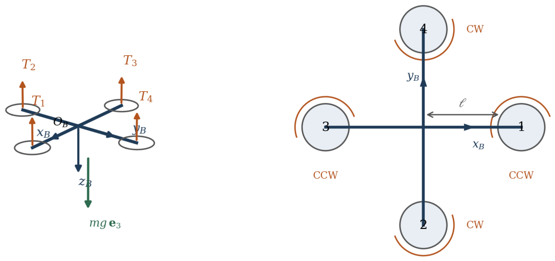
Figure 2.
Directional attitude-robustness framework. A body-frame disturbance with a constant horizontal magnitude of 8 N and a fixed vertical component of N is applied at an offset centre of pressure.
Figure 2.
Directional attitude-robustness framework. A body-frame disturbance with a constant horizontal magnitude of 8 N and a fixed vertical component of N is applied at an offset centre of pressure.
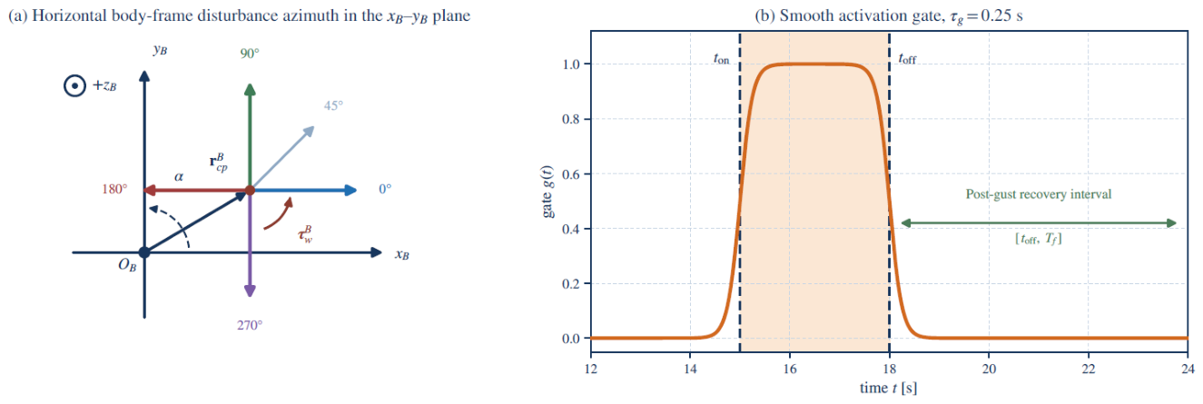
Figure 3.
Cascaded closed-loop architecture used for all controller configurations. The position controller and yaw-compensated tilt-and-thrust mapping are common to all configurations; only the inner attitude controller is replaced.
Figure 3.
Cascaded closed-loop architecture used for all controller configurations. The position controller and yaw-compensated tilt-and-thrust mapping are common to all configurations; only the inner attitude controller is replaced.
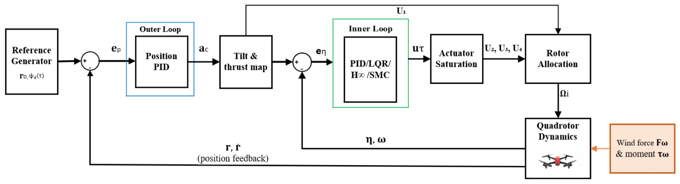
Figure 4.
Directional roll/pitch failure-angle sweep protocol. For each wind azimuth, the disturbance force and centre-of-pressure moment are constructed, the attitude-only model is simulated, and the resulting excursion, recovery, effort, and saturation metrics are used for directional classification.
Figure 4.
Directional roll/pitch failure-angle sweep protocol. For each wind azimuth, the disturbance force and centre-of-pressure moment are constructed, the attitude-only model is simulated, and the resulting excursion, recovery, effort, and saturation metrics are used for directional classification.
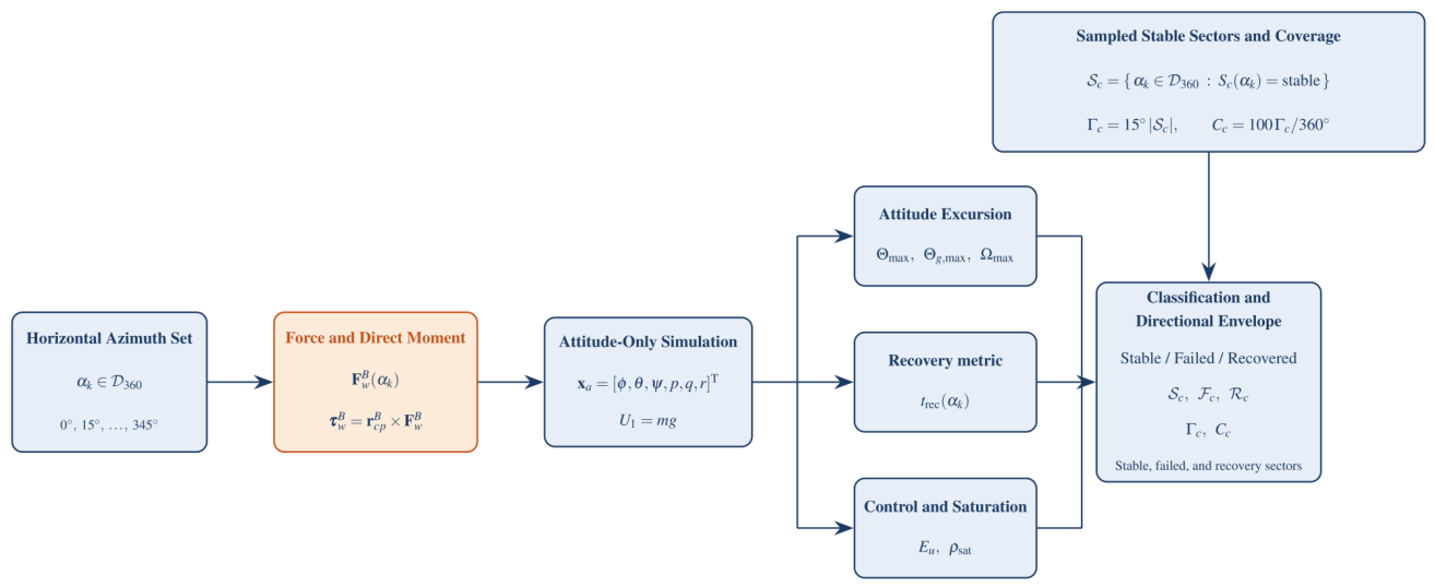
Figure 5.
Nominal position and attitude step responses of the baseline and PSO-optimized controller pairs for , , , , and .
Figure 5.
Nominal position and attitude step responses of the baseline and PSO-optimized controller pairs for , , , , and .
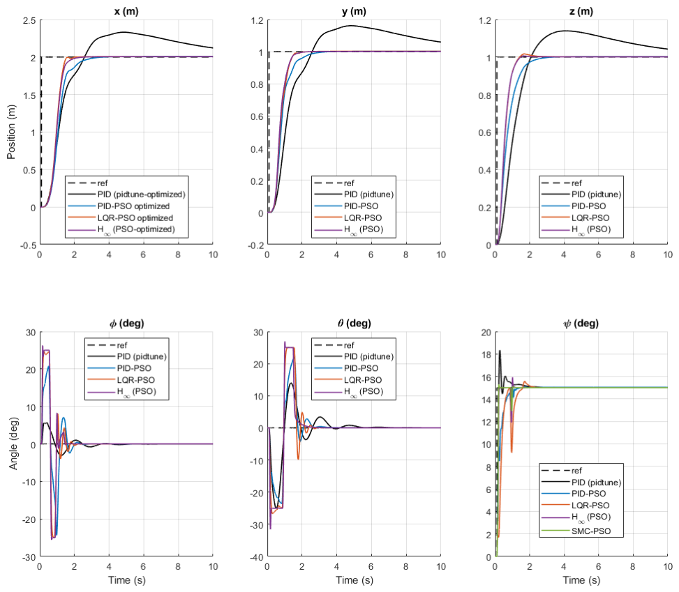
Figure 6.
Position and attitude responses under a body-frame wind disturbance applied during (D1 scenario).
Figure 6.
Position and attitude responses under a body-frame wind disturbance applied during (D1 scenario).
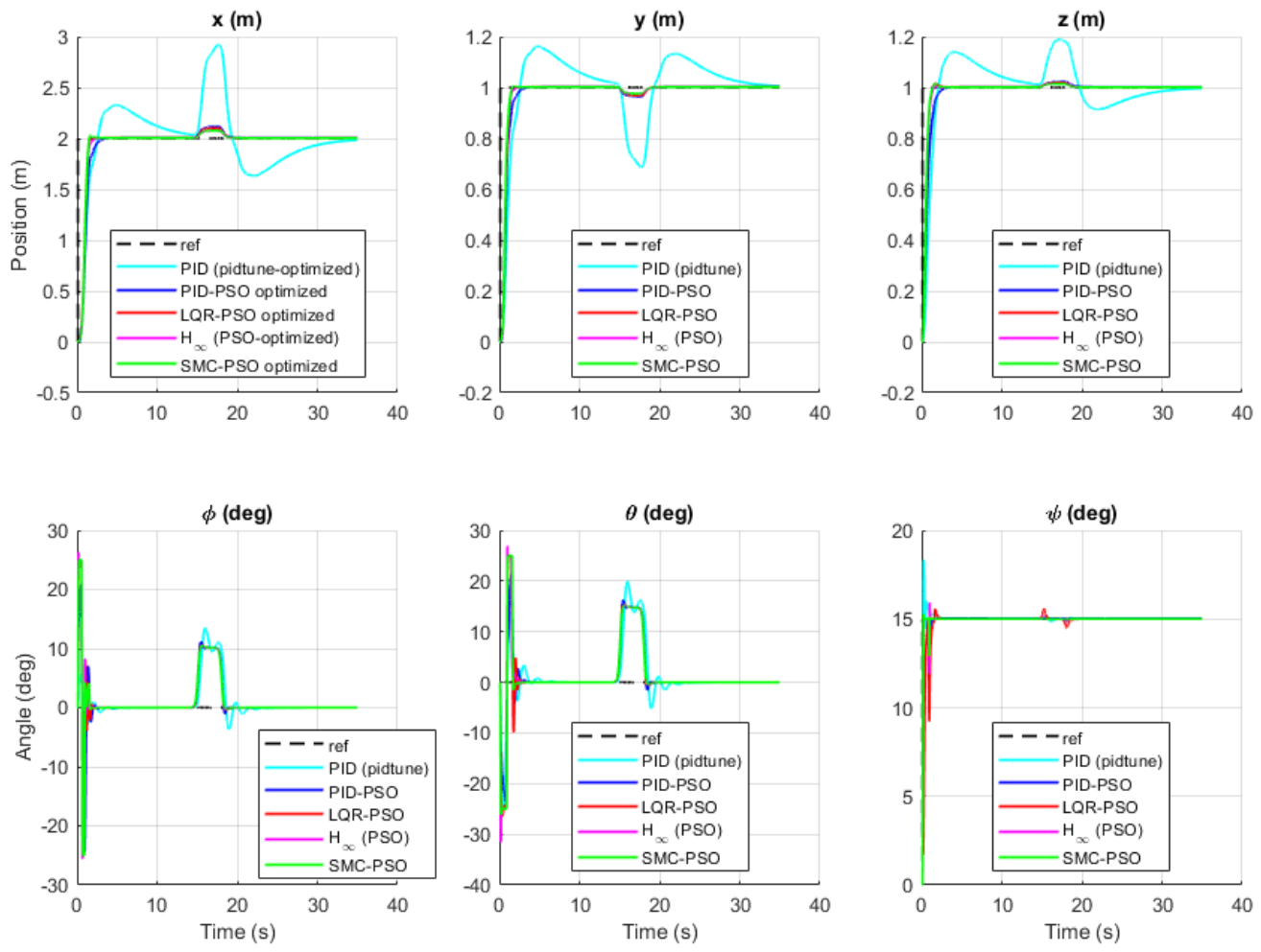
Figure 7.
Helical-path tracking under wind disturbance: (a) departure from the initial position, (b) tracking during the wind-disturbance interval, and (c) arrival at the final position.
Figure 7.
Helical-path tracking under wind disturbance: (a) departure from the initial position, (b) tracking during the wind-disturbance interval, and (c) arrival at the final position.
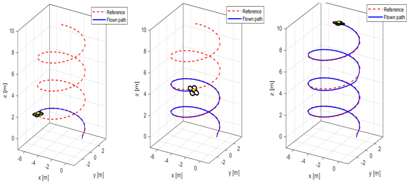
Figure 8.
Three-dimensional helical trajectories obtained using the PSO-optimized PID, LQR, , and SMC controllers under the D2 wind disturbance.
Figure 8.
Three-dimensional helical trajectories obtained using the PSO-optimized PID, LQR, , and SMC controllers under the D2 wind disturbance.
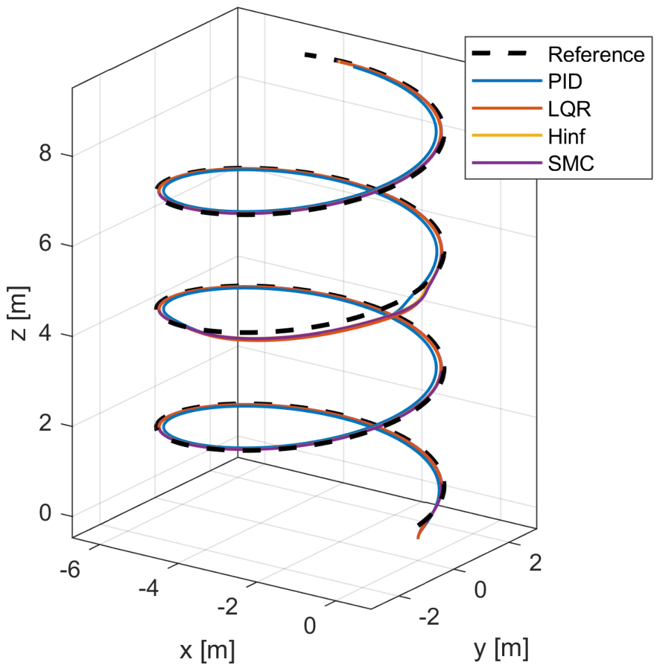
Figure 9.
Position and attitude responses during helical-trajectory tracking under a body-frame wind disturbance applied during (D2 scenario).
Figure 9.
Position and attitude responses during helical-trajectory tracking under a body-frame wind disturbance applied during (D2 scenario).
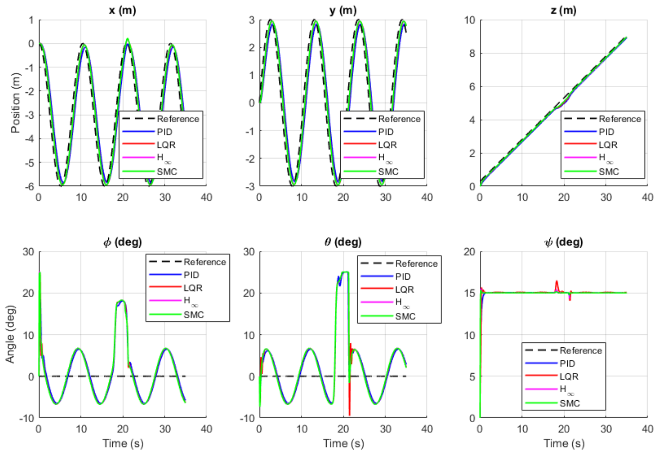
Figure 10.
Control response of the optimized LQR controller during D2: wind-force components (top), control-input magnitudes (middle), and instantaneous and cumulative normalized control effort (bottom).
Figure 10.
Control response of the optimized LQR controller during D2: wind-force components (top), control-input magnitudes (middle), and instantaneous and cumulative normalized control effort (bottom).
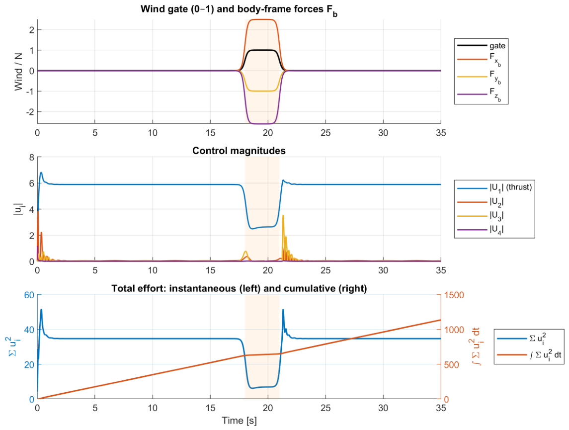
Figure 11.
Maximum geometric tilt versus horizontal wind azimuth for the four optimized controllers.
Figure 11.
Maximum geometric tilt versus horizontal wind azimuth for the four optimized controllers.
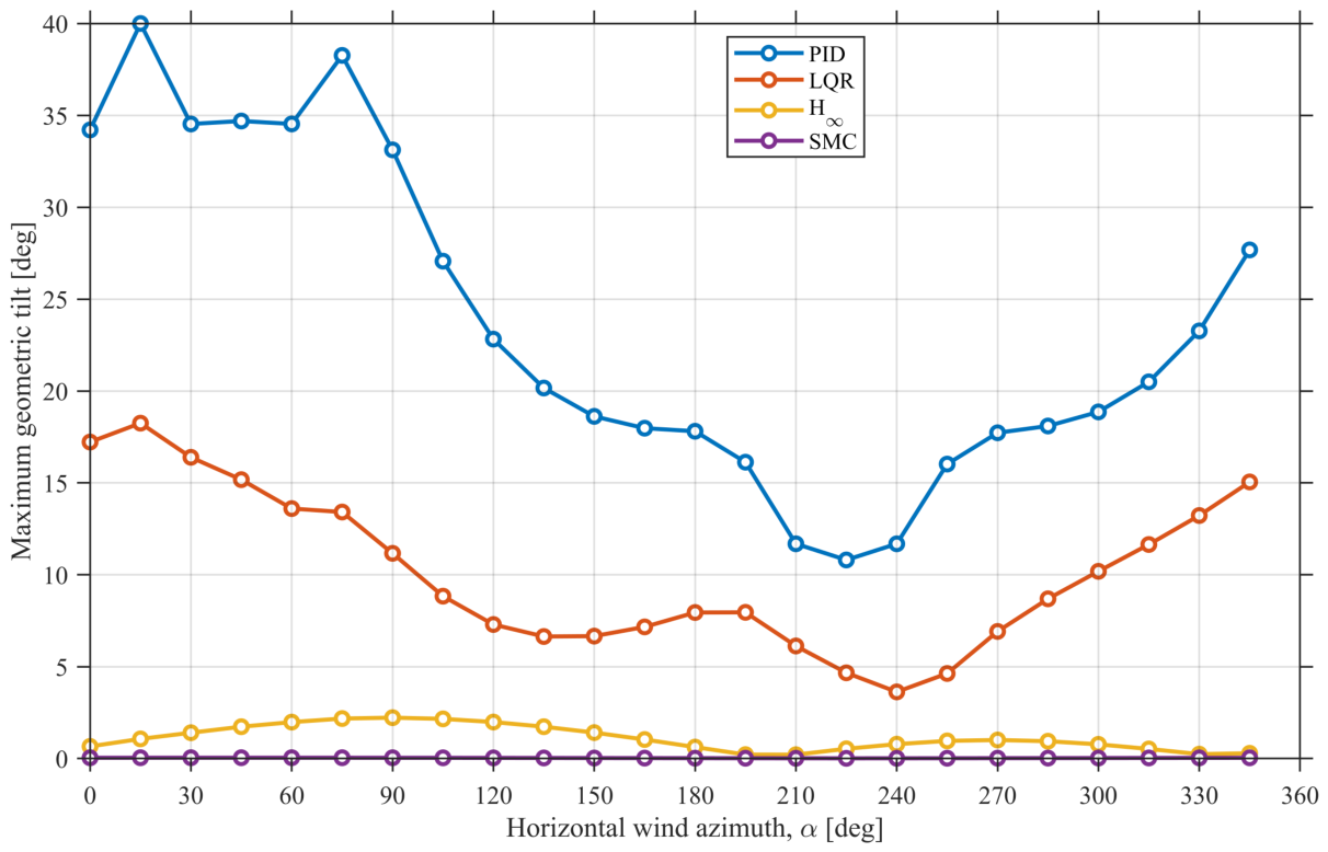
Figure 12.
Maximum individual-axis roll–pitch excursion across the complete wind-direction sweep, with the safe-excursion and near-flip boundaries.
Figure 12.
Maximum individual-axis roll–pitch excursion across the complete wind-direction sweep, with the safe-excursion and near-flip boundaries.
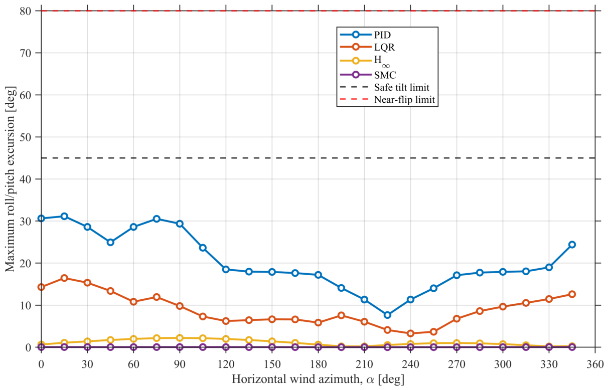
Figure 13.
Directional geometric-tilt envelopes: (a) comparison of all controllers and (b) enlarged and SMC responses.
Figure 13.
Directional geometric-tilt envelopes: (a) comparison of all controllers and (b) enlarged and SMC responses.
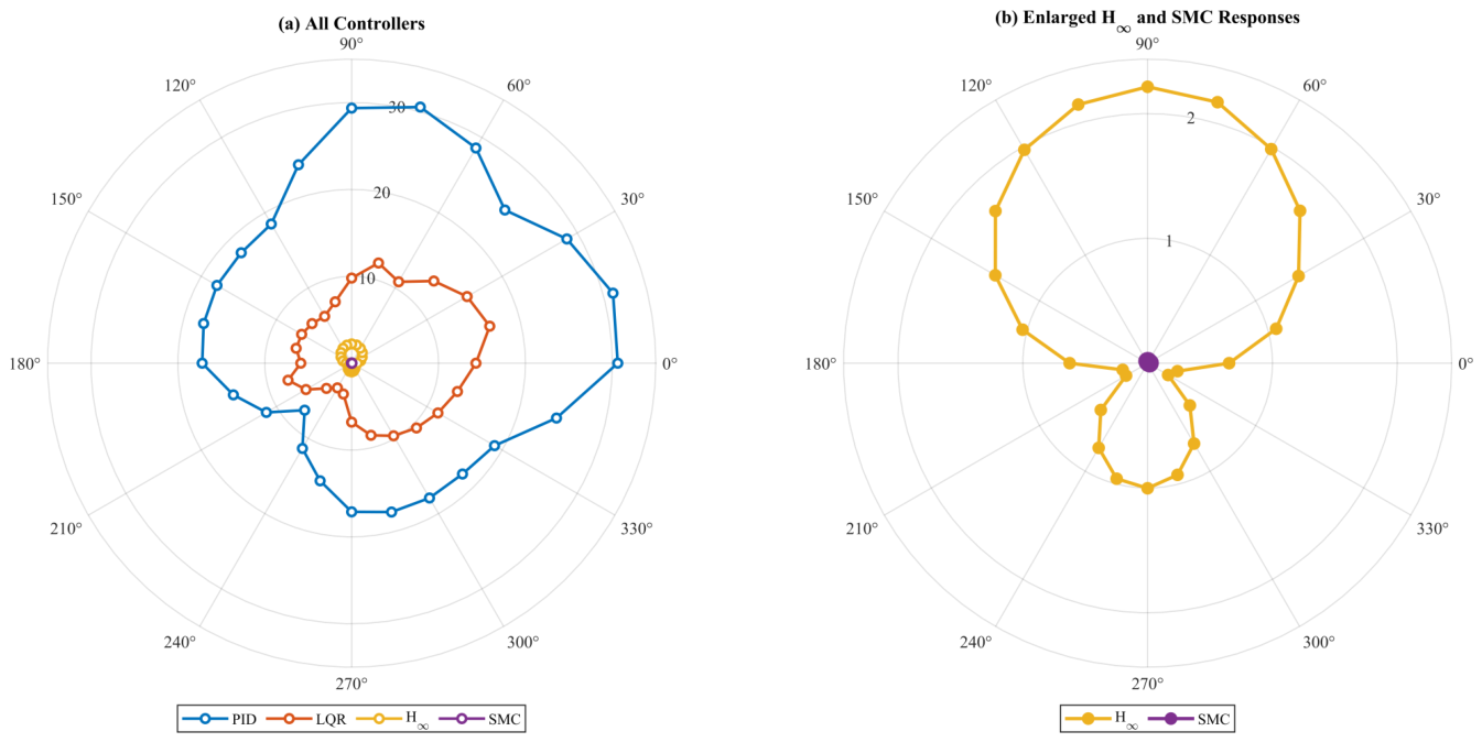
Figure 14.
Directional comparison of (a) differential attitude-control effort and (b) actuator-saturation duty, including the 35% protocol threshold.
Figure 14.
Directional comparison of (a) differential attitude-control effort and (b) actuator-saturation duty, including the 35% protocol threshold.
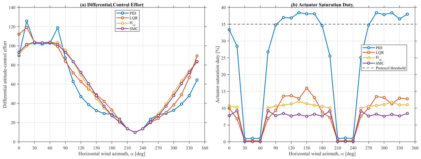
Figure 15.
Directional robustness maps: (a) stability classification, (b) post-disturbance recovery over the wind sweep.
Figure 15.
Directional robustness maps: (a) stability classification, (b) post-disturbance recovery over the wind sweep.
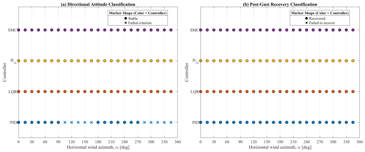
Table 1.
Principal notation.
| Symbol | Definition | Unit |
|---|---|---|
| Inertial position | m | |
| Inertial velocity | ||
| Euler angles | rad | |
| Body angular velocity | ||
| Body-to-inertial rotation matrix | – | |
| Euler-rate transformation | – | |
| Collective thrust | N | |
| Roll/pitch differential thrust | N | |
| Yaw moment | ||
| Rotor angular speed | ||
| Body-frame disturbance force | N | |
| Body-frame disturbance moment | ||
| m | Mass | kg |
| J | Inertia matrix | |
| Rotor polar inertia | ||
| ℓ | Arm length | m |
| b | Thrust coefficient | |
| d | Drag-torque coefficient |
Table 2.
Physical and actuator parameters of the simulated quadrotor.
| Parameter | Symbol | Value | Unit |
|---|---|---|---|
| Mass | m | kg | |
| Gravitational acceleration | g | ||
| Roll moment of inertia | |||
| Pitch moment of inertia | |||
| Yaw moment of inertia | |||
| Rotor polar moment of inertia | |||
| Arm length | ℓ | m | |
| Thrust coefficient | b | ||
| Drag-torque coefficient | d | ||
| Translational damping coefficient | |||
| Rotational damping coefficient | |||
| Maximum collective thrust | N | ||
| Maximum roll/pitch differential thrust | N | ||
| Maximum yaw moment | |||
| Maximum roll/pitch moment |
Table 3.
Decision variables and admissible parameter bounds for each controller configuration.
| Configuration | Decision vector | Bounds | |
|---|---|---|---|
| PID–PID | 8 | ||
| PID–LQR | 12 | ||
| PID– | 12 | ||
| PID–SMC | 6 |
Table 4.
Numerical integration and simulation settings.
| Setting | Value |
|---|---|
| Solver | Explicit adaptive Dormand–Prince (ode45) for all controllers |
| D1 numerical settings | Relative/absolute tolerances: |
| D2 numerical settings | Relative/absolute tolerances: ; maximum step and output interval: s |
| D3 numerical settings | Relative/absolute tolerances: ; event-based termination |
| Tuning horizon | 20 s for GA and PSO |
| Nominal step horizon | 10 s |
| Disturbed step horizon | 35 s |
| Helical-trajectory horizon | 35 s |
| D1/D2 initial state | ; controller states initialized to zero |
| D3 initial state | , |
| Optimizer repeatability | Fixed random seed; one retained run per optimizer–controller pair |
Table 6.
Summary of the controller optimization results and selected configurations.
| Controller | Baseline J | GA Best J | PSO Best J | PSO Improvement | Selected Method |
|---|---|---|---|---|---|
| PID | 121.58 | 65.33 | 11.70 | 90.38% | PSO |
| LQR | 848.05 | 20.51 | 9.54 | 98.88% | PSO |
| 1293.14 | 7.31 | 5.23 | 99.60% | PSO | |
| SMC | – | 4.50 | 4.28 | 4.89%* | PSO |
| *Improvement of PSO relative to the GA solution because no separate baseline SMC result was used. | |||||
Table 7.
Aggregated nominal step-response performance of the baseline and PSO-optimized controllers.
Table 7.
Aggregated nominal step-response performance of the baseline and PSO-optimized controllers.
| Controller | Position response | Attitude response | ||||||||
|---|---|---|---|---|---|---|---|---|---|---|
| (s) | (s) | (%) | IAE | ITAE | (s) | (s) | (%) | IAE | ITAE | |
| PID–PID baseline | 1.614 | – | 16.56 | 7.47 | 22.10 | 0.074 | 4.994 | 22.24 | 0.598 | 0.680 |
| PID–PID PSO | 1.149 | 2.504 | 0.39 | 3.58 | 2.59 | 0.436 | 2.496 | 4.37 | 0.855 | 0.702 |
| PID–LQR PSO | 0.745 | 1.404 | 1.68 | 2.96 | 1.70 | 0.420 | 2.456 | 3.80 | 1.090 | 0.777 |
| PID– PSO | 0.732 | 1.671 | 0.59 | 2.98 | 1.64 | 0.083 | 2.072 | 6.21 | 0.987 | 0.639 |
| PID–SMC PSO | 0.679 | 1.353 | 1.62 | 2.93 | 1.59 | 0.067 | 1.859 | 1.92 | 1.020 | 0.700 |
Table 8.
Aggregated performance under the D1 finite-duration wind disturbance.
| Controller | Position response | Attitude response | ||||||||
|---|---|---|---|---|---|---|---|---|---|---|
| (s) | (s) | (%) | IAE | ITAE | (s) | (s) | (%) | IAE | ITAE | |
| PID–PID baseline | 1.610 | 31.626 | 46.14 | 16.10 | 193.0 | 0.074 | 21.082 | 22.24 | 2.17 | 27.3 |
| PID–PID PSO | 1.149 | 18.350 | 5.81 | 4.36 | 17.2 | 0.436 | 18.570 | 4.37 | 2.20 | 22.8 |
| PID–LQR PSO | 0.745 | 18.309 | 5.05 | 3.60 | 13.4 | 0.420 | 18.182 | 3.92 | 2.42 | 22.6 |
| PID– PSO | 0.732 | 18.227 | 3.80 | 3.46 | 10.7 | 0.083 | 18.228 | 6.21 | 2.30 | 22.3 |
| PID–SMC PSO | 0.679 | 18.202 | 3.80 | 3.41 | 10.5 | 0.067 | 18.228 | 1.92 | 2.34 | 22.3 |
Table 9.
Performance comparison for helical-trajectory tracking under the D2 wind disturbance.
| Controller | RMSE | MAE | IAE | ISE | Wind RMSE | |||||
|---|---|---|---|---|---|---|---|---|---|---|
| (m) | (m) | (m s) | (m2 s) | (m) | (m) | (s) | (deg) | (deg) | (s) | |
| PID | 1.0790 | 1.0759 | 37.658 | 40.748 | 1.0253 | 1.0913 | 1.39 | 30.417 | 30.417 | 3.7113 |
| LQR | 0.7661 | 0.7648 | 26.769 | 20.540 | 0.7302 | 0.8000 | 1.21 | 30.611 | 30.611 | 3.6910 |
| 0.7188 | 0.7178 | 25.122 | 18.084 | 0.6886 | 0.7414 | 1.31 | 30.607 | 30.607 | 3.7648 | |
| SMC | 0.6768 | 0.6760 | 23.659 | 16.034 | 0.6470 | 0.7083 | 1.23 | 30.616 | 30.616 | 3.7942 |
Table 10.
Directional roll–pitch attitude-robustness summary.
| (a) Directional classification and attitude metrics | ||||||
|---|---|---|---|---|---|---|
| Controller | Stable coverage |
Worst geometric tilt |
Worst individual-axis excursion |
Worst direction |
Maximum saturation |
Worst recovery |
| (%) | (deg) | (deg) | (deg) | (%) | (s) | |
| PID | 58.33 | 39.997 | 31.141 | 15 | 38.452 | 0.481 |
| LQR | 100 | 18.251 | 16.454 | 15 | 15.964 | 0.202 |
| 100 | 2.225 | 2.214 | 90 | 11.971 | ||
| SMC | 100 | 0.046 | 0.040 | 45 | 9.222 | |
| (b) Angular-rate and control metrics | ||||||
| Controller |
(rad s−1) |
(rad s−1) |
(rad s−1) |
(rad s−1) |
(–) |
|
| PID | 8.140 | 7.975 | 22.420 | 8.196 | 53.921 | |
| LQR | 3.024 | 2.547 | 16.376 | 3.244 | 59.003 | |
| 0.353 | 0.702 | 26.805 | 0.768 | 59.805 | ||
| SMC | 0.011 | 0.011 | 18.682 | 0.012 | 59.836 |
Note: Classification uses Θexc,max; Θg,max is diagnostic. Component-rate maxima are independent and may occur at different
times or azimuths.
Disclaimer/Publisher’s Note: The statements, opinions and data contained in all publications are solely those of the individual author(s) and contributor(s) and not of MDPI and/or the editor(s). MDPI and/or the editor(s) disclaim responsibility for any injury to people or property resulting from any ideas, methods, instructions or products referred to in the content. |
© 2026 by the authors. Licensee MDPI, Basel, Switzerland. This article is an open access article distributed under the terms and conditions of the Creative Commons Attribution (CC BY) license (http://creativecommons.org/licenses/by/4.0/).
Copyright: This open access article is published under a Creative Commons CC BY 4.0 license, which permit the free download, distribution, and reuse, provided that the author and preprint are cited in any reuse.