
Submitted:
16 September 2026
Posted:
16 September 2026
You are already at the latest version
Abstract
The \(k\)-SAT problem is a canonical NP-complete problem for which no efficient algorithm is known. This paper proposes a hybrid quantum–classical algorithm that employs Grover's algorithm as the inner local search of a randomized outer loop. Each outer iteration measures a random assignment, prepares a problem-dependent superposition over the Hamming ball of radius \(r\) around it, and applies amplitude amplification to locate a satisfying assignment. Because the ball center is measured, the outer loop remains a classical repetition over independently sampled balls and contributes the inverse success probability rather than its square root; balancing this against the inner quadratic speedup shifts the optimal radius from \(n/(k+1)\) to \(n/(1+\sqrt{k})\) and yields the running time $(2-2/(1+\sqrt{k}))^{n}$, up to polynomial factors—\(1.268^{n}\) for \(k=3\), below the best known classical \(1.307^{n}\). The contribution is not an asymptotic record—the best known quantum exponents for \(k\)-SAT, obtained by amplifying stronger classical solvers as black boxes, remain smaller—but a fully explicit, gate-level construction: the problem-dependent state over the Hamming ball and the \(k\)-SAT oracle are decomposed into elementary quantum gates, and the polynomial gate and qubit overheads are accounted for in full.
Keywords:
k-SAT problem
; Grover’s algorithm
; amplitude amplification
; quantum local search
; Hamming ball
; hybrid quantum–classical algorithm
; gate-level construction
1. Introduction
The k-SAT problem () is a canonical NP-complete problem [1], and no polynomial-time algorithm for it is known. Classical algorithms for k-SAT fall broadly into two categories: deterministic and probabilistic. Deterministic approaches typically rely on divide-and-conquer, exhaustive search, or backtracking, while probabilistic methods often employ local search heuristics. The worst-case time complexity of state-of-the-art algorithms in both categories is generally , where n is the number of Boolean variables and is a constant base. Since a smaller implies lower computational complexity, much research [2,3,4] has focused on minimizing this exponential base.
On the probabilistic side, Paturi, Pudlák, and Zane [2] introduced the PPZ algorithm in 1997, achieving a randomized upper bound significantly below . Schöning [3] subsequently proposed a simple local search algorithm with expected running time , yielding , which improved upon the earlier PPZ bound of Ref. [2]. Hofmeister et al. [5] later refined Schöning’s approach, reducing the 3-SAT complexity to . Meanwhile, Paturi et al. [6] enhanced the original PPZ framework into the PPSZ algorithm, achieving for unique 3-SAT (the variant with exactly one satisfying assignment). Hertli [7] subsequently extended this analysis, proving that the PPSZ bound under the uniqueness assumption applies equally to general 3-SAT. More recently, Hansen et al. [8] introduced a biased variant of PPSZ, further improving the unique 3-SAT bound to .
Parallel to these randomized advances, significant effort has been devoted to derandomization and deterministic algorithm design. Dantsin et al. [9] showed how to simulate Schöning’s random walk deterministically, at the price of a mildly larger base: their Hamming-ball local search runs in time , i.e., for . For 3-SAT specifically, they introduced a tailored local search strategy that further reduced the bound to . Moser and Scheder [10] later completed the full derandomization of Schöning’s algorithm using limited independence. Brueggemann and Kern [4] refined the local search strategy of Dantsin et al., reducing the 3-SAT complexity to . Scheder [11] further improved this bound to . To the best of our knowledge, the current best deterministic algorithm for 3-SAT remains that of Kutzkov and Scheder [12], achieving . Despite over a decade of effort, no improvement has been found, highlighting the need for fundamentally new paradigms.
Quantum algorithms have demonstrated advantages over classical counterparts in several computational tasks, including integer factorization, unstructured search, and search on graphs [13,14,15], and they are by now a standard tool in application areas such as machine learning and combinatorial optimization [16,17,18]. Motivated by these developments, we investigate the application of quantum computation to the k-SAT problem. Prior quantum approaches to k-SAT largely accelerate an existing classical solver while keeping its structure inside a black-box oracle. Grover’s algorithm alone yields [14]. Combining Grover search with the then best classical 3-SAT algorithm ( [5]) lowers the exponent to [19], and applying amplitude amplification [20] to the PPSZ algorithm [6,7,8] gives for 3-SAT. These are, to our knowledge, the strongest known exponents for worst-case k-SAT in the gate model. Inspired by the classical algorithm in [3], we propose a hybrid quantum-classical algorithm that employs Grover’s algorithm as a local search subroutine for solving k-SAT. The proposed algorithm is a hybrid quantum-classical procedure: its outer loop classically samples local search spaces, while its inner loop performs quantum search. It proceeds in t outer iterations. In each iteration, a problem-dependent superposition state is constructed over a local search space—specifically, a Hamming ball of radius r centered at a randomly generated assignment—by exploiting the problem structure. Grover’s algorithm is then applied to this state in its amplitude-amplification form—the number of solutions inside a ball is not known in advance, so the exponential-search variant is used—to search for a satisfying assignment. Because the outer loop is a classical repetition over independently sampled balls, the number of outer iterations is governed by the classical success probability, and the resulting running time is (with the optimal radius ), which improves upon the classical local-search bounds for k-SAT [3,9] and, at , upon the best known classical algorithm [8] ( versus ; see Section 3.6 for the general-k comparison). These gains are over classical solvers: black-box amplification of a stronger classical solver yields smaller quantum exponents [6,8,19,20].
The contributions of this work can be summarized as follows.
- An explicit, gate-level construction. Both the problem-dependent superposition over the Hamming ball and the k-SAT oracle are decomposed into elementary gates, so that no black-box oracle is left in the complexity and the polynomial overhead is fixed at gates in total.
- A hybrid framework with a re-optimized ball radius. Because the center of each ball is measured, the outer loop is a classical repetition over independently sampled balls and contributes the inverse success probability rather than its square root; balancing this factor against the quadratic speedup of the inner search shifts the optimal radius from the classical to , so that the classical repetition does not simply reproduce the classical Hamming-ball exponent.
- A complete accounting and a numerical verification. The qubit and gate costs of the whole construction are counted, and the two bounds on which the exponent rests—the success probability of a ball and the marked amplitude of the constructed state—are checked numerically for on small planted instances (Section 4).
The remainder of this paper is organized as follows. Section 2 introduces the k-SAT problem, defines quantum analogues of the three fundamental classical logic gates involved, and reviews Grover’s algorithm. Section 3 presents the proposed algorithm, beginning with an overview of the framework, followed by the construction of the problem-dependent state and the decomposition of the Grover oracle for k-SAT into elementary quantum gates. The section concludes with an analysis of the algorithm’s feasibility and time complexity and with a comparison against prior quantum algorithms. Section 4 reports the numerical verification of the two bounds entering the exponent; Section 5 offers concluding remarks, and the Appendix details the gate-level implementation of the conditional neighborhood expansion.
2. Preliminaries
2.1. Definition of the k-SAT Problem
The k-SAT problem in conjunctive normal form (CNF) is defined as follows. Let be a finite set of n Boolean variables, and let be a set of m clauses. Each clause is given by , where each is called a literal; for simplicity, the k literals of a clause are assumed to involve k distinct variables, so that no clause contains both and . This is the case considered throughout, and it is what makes the k branches generated by [Equation (5)] distinct. The k-SAT problem asks whether there exists an assignment, such that the formula is satisfied. If is satisfied by a, then a is called a satisfying assignment of .
Note that for fixed n and m, each distinct set of clauses defines a unique instance of the k-SAT problem. Throughout, m is taken to be polynomially bounded in n, so that the clause count contributes only a polynomial factor to all running times reported below. In classical computation, a Boolean variable takes a binary value of either 0 (false) or 1 (true), and logical operations act on one or more such variables. By analogy, a quantum truth value can be defined as a superposition of the basis states 0 and 1. A quantum logical variable assumes such a quantum truth value and is naturally represented by a qubit, whose state encodes this value. Consequently, a quantum logical operation is defined as a quantum gate acting on one or more qubits, transforming their joint quantum state.
The k-SAT problem involves n Boolean variables, each taking a value in . Consequently, there are possible assignments, which constitute the search space . Each assignment can be encoded as a computational basis state , where . In the remainder of this paper, we identify each classical assignment with its corresponding computational basis state.
2.2. Quantum Realizations of Logic Gates: NOT, AND, and OR
As shown above, the k-SAT problem is built upon three basic logical operations: (∧), (∨), and (¬). Their quantum analogues, denoted as , , and , are defined as follows.
The classical operation maps and . Its quantum analogue, , is defined by its action on the computational basis:
This operator is equivalent to the single-qubit Pauli-X gate, which flips .
The classical gate () embeds into a reversible three-qubit operator :
This is precisely the Toffoli gate, which applies a bit-flip to the third qubit if and only if the first two qubits are both 1.
The classical operation acts on two Boolean variables, yielding 0 if and only if both inputs are 0. Its reversible quantum analogue, , is defined on three qubits as:
where ⊕ denotes addition modulo 2. This operation flips the target qubit conditioned on at least one of the control qubits or being 1. The gate can be implemented via and . Specifically, one applies to each of the first two qubits, then to all three qubits, and finally to each of the three qubits.
2.3. Grover’s Algorithm
In Grover’s algorithm, the Grover iteration is applied times to the system state, where is the search space size (n being the number of qubits) and M is the number of solutions. The qubits are then measured in the computational basis, which returns a solution with probability ; repeating the whole procedure times raises the success probability to at least .
The Grover iteration consists of the following four steps:
- Apply the oracle O: , where if x is a solution and otherwise. This marks the solution states by flipping their phases.
- Apply the Hadamard transform .
- Apply the diffusion operator , which reflects the state about |0⟩ (equivalently, flips the phase of all non-zero computational basis states).
- Apply the Hadamard transform .
Using the identity , where is the equal superposition state, the Grover iteration simplifies to
where O is the oracle defined in Step 1.
If an oracle is available that marks the solution states of a given problem, Grover’s algorithm can solve it without exploiting additional problem-specific structure beyond the oracle itself. In particular, for the k-SAT problem, assuming such an oracle exists and the instance has a unique solution (), Grover’s algorithm achieves a time complexity of . This provides a quadratic speedup over exhaustive classical search and outperforms the best known classical deterministic algorithms for k-SAT, though it remains slower than state-of-the-art probabilistic solvers. Nevertheless, incorporating problem structure into the quantum algorithm can further reduce the complexity, as demonstrated in the subsequent analysis.
3. The Proposed Algorithm
3.1. Algorithm Framework
The proposed algorithm is a hybrid quantum-classical procedure whose outer loop performs t classically repeated iterations, each consisting of the following three steps:
- Random assignment generation. Prepare the uniform superposition state by applying to n qubits initialized in , then measure all qubits in the computational basis to obtain a random assignment .
- Subspace state preparation. Construct a problem-dependent quantum state starting from the randomly generated assignment a.
- Grover search within subspace. Apply Grover’s algorithm to to search for a solution to the k-SAT instance.
3.2. Construction of the Problem-Dependent State
The problem-dependent state is constructed by applying the following two procedures iteratively r times, starting from the randomly generated assignment a; throughout this section, denotes the state of the round being considered.
-
Clause evaluation (E). This procedure computes the quantum truth value of each clause in the k-SAT instance. For a clause , we introduce auxiliary qubits , all initialized to 0. Let denote the qubit corresponding to literal . The quantum OR operation () is applied sequentially: first to , , and ; then to , , and ; and so on, until finally to , , and . The final result is stored in . Across all m clauses, this requires auxiliary qubits, with the truth values of clauses stored in , respectively.The full clause-evaluation operator is defined aswhere denotes the sequence of gates applied to clause , as described above. After applying E, the state of the current round becomes entangled with each clause register aswhere and are the (unnormalized) components of that state supported on the subspaces in which clause evaluates to false and true, respectively.
-
Conditional neighborhood expansion (F). This procedure applies a conditional transformation to each computational basis state in the superposition , expanding the neighborhood of one unsatisfied clause. Let be the index of the first clause that is false under a, and let denote conditioning on the clause-register pattern in which clauses are true and clause is false, i.e., the multiply-controlled unitary that acts as the identity unless the clause registers hold that pattern and that applies the operation in its argument whenever they do. The conditional expansion operator is defined as the product of these controlled unitaries,where is the expansion operator associated with clause . The m control patterns are mutually exclusive—no assignment can have two first-false clauses—and the expansion changes only the assignment and label registers, so the clause registers are left untouched while a factor acts and, on any computational basis state, at most one factor of Equation (3) differs from the identity; the factors therefore commute. Equivalently, on a basis state of the clause registers F reduces to the direct sum of the unitaries , one summand for each sector in which clause is the first clause that is false, together with the identity on the sector in which all clauses are true: an individual summand is only a partial isometry, and it is the completeness of the mutually exclusive sectors that makes the operator F unitary. Each factor is a controlled unitary, and hence unitary, by construction, and so is their product. On a computational basis state whose clause registers hold the values , exactly one sector is selected—the expansion of the first clause that is false, i.e., of clause —whereas if a satisfies every clause no expansion takes place, in which case F acts as the identity on the assignment and label registers. Thus F performs a single k-way branching per round instead of a simultaneous expansion of all m clauses. This mirrors the branching step of a classical local search, in which a single unsatisfied clause is selected and each of its k literals is tried in turn; applying instead the expansion of every false clause—each controlled by the single clause —would generate branches in a single round for an assignment with false clauses and would not correspond to the classical search tree. The circuit implementation of F is illustrated in Figure 1.Each block acts on the assignment register and on an auxiliary label register s of qubits, initialized to : a unitary W first prepares a uniform superposition over k basis states of s, which then controls a Pauli- flip of the corresponding literal,where prepares the uniform superposition in s, the label values being understood cyclically, , so that the basis states of s are indexed by ; the second sum then acts as the identity on the unused label values , which for is the single all-zero label (cf. Appendix A) and is empty when , so that it completes the first factor to a unitary on the whole register space. flips the variable to which the literal refers. Acting on an assignment a that falsifies , this block giveswhere denotes the assignment obtained by flipping the bit corresponding to literal in a. Each differs from a in exactly one bit position and satisfies , so maps a to a uniform, coherent superposition over its k Hamming-distance-1 neighbors that satisfy , with the chosen branch recorded in the label register s. This label is retained rather than uncomputed, and no unitary can do otherwise: the corresponding map on the assignment register alone, , is not an isometry—for and it gives , and the obstruction persists for inside the sector where is active: were the label reset, the falsifying input 000 would keep a component of amplitude on , the very state that the control leaves untouched for the orthogonal input 100—so no unitary that generates Equation (5) can also return s to . Consequently each of the r rounds of the construction employs its own label register (and, in the case , its own copy of the auxiliary register w of Appendix A), and each round keeps its own copy of the clause registers as well, since these cannot be uncomputed either (see the discussion of Equation (6)). We provide an implementation scheme of using elementary quantum gates in Appendix A.
The full construction procedure can then be written as
where denotes the clause-evaluation operator [Equation (2)] acting on the i-th copy of the clause registers, which starts in , and the conditional neighborhood expansion [Equation (3)] controlled by those registers and acting on the label register of the i-th round. In each round the quantum truth values of all clauses are first computed by for the assignment currently held in the assignment register, and the conditional neighborhood expansion is then applied on the basis of these truth values. Unlike the oracle of Equation (9), the expansion changes the assignment register, so the clause registers of a round cannot be uncomputed by : applying after the expansion computes the clause values of the new assignment on top of those of the previous one, and the registers return to 0 only when the assignment register is left unchanged—which holds for the oracle but not here. Like the branch label of F [Equation (5)], they are therefore retained rather than uncomputed and reused. This iterative process leverages the clause structure of the k-SAT instance to transform the initial random assignment into a problem-dependent superposition. The resulting state is supported on basis states of the form , tensored with the retained clause registers, in which x lies in the Hamming ball and the labels record the k-way choices taken along the corresponding branch of the search tree, so that the state forms a local search subspace tailored to the problem instance.
Remark on unitarity. All the operators employed above are unitary: , , and act as permutations of the computational basis (and are self-inverse); the Hadamard transform H and are Hermitian and satisfy ; W is a state-preparation unitary [Equation (4) and Appendix A]; E [Equation (2)], [Equation (7)], [Equation (4)] and F [Equation (3)] are products of multiply-controlled unitaries, each control condition being a computational-basis pattern on the clause registers (so that the operator reduces to a direct sum of unitaries over the mutually exclusive sectors), and the same holds for the construction C [Equation (6)], the oracle O [Equation (9)] and the Grover iteration G [Equation (1)]. Within the construction, the only non-unitary object in the analysis is the branch-and-forget map introduced below Equation (5), which is not an executed operation but the shortcut of discarding the branch labels: its failure to be an isometry is precisely why the label registers—and, as explained above, the clause registers of each round—are retained and never discarded, so that every step of the construction is a unitary gate. Non-unitary operations occur only where the algorithm measures—in generating the random assignment in Step 1, in the intermediate checks performed by the exponential-search variant of amplitude amplification in Step 3, and in the final readout—and it is the measurement in Step 1 that keeps the outer loop over balls a classical repetition.
3.3. Oracle for the k-SAT Problem
In this subsection, we decompose the oracle O into elementary quantum operations. As previously described, the oracle O identifies solution states and flips their phases. To detect these states, we first apply the clause-evaluation operator E [Equation (2)] to compute the quantum truth values of all m clauses. Subsequently, the quantum AND operation () is applied sequentially times to evaluate the entire formula . This formula-evaluation procedure is defined as
where are auxiliary qubits initialized to 0, and denotes the gate acting on qubits x, y, and z. This step requires auxiliary qubits in total, with the final truth value of stored in .
Writing the collection of labels produced by the construction as l, the problem-dependent state can be decomposed into two orthogonal components based on the value of :
where and are unnormalized and span the subspaces corresponding to unsatisfying and satisfying assignments, respectively (the label and clause registers of the construction are spectators: the oracle below acts as the identity on them and uses its own clause and formula registers, initialized to 0, so the marking condition depends only on the assignment). After applying the clause-evaluation operator E [Equation (2)] and the formula-evaluation operator [Equation (7)], the system becomes entangled with the ancilla qubit :
Finally, a controlled-NOT () gate is applied to the ancilla qubits (control) and (target), where is initialized to . This operation transforms the entangled state into
The complete oracle for the k-SAT problem is then given by
where and are the inverses of the clause-evaluation operator E [Equation (2)] and the formula-evaluation operator [Equation (7)], respectively. These uncomputation steps restore the clause and formula registers to their initial states, ensuring that the oracle acts as a pure phase oracle on the computational basis; it is the identity on the label and clause registers of the construction.
3.4. Reachability within Hamming Balls
Suppose is a satisfying assignment. We now show that after r iterations of the construction procedure [Equation (6)], the state has amplitude at least on the marked subspace, i.e., on the components of Equation (8) whose assignment register holds a satisfying assignment. The Hamming distance between two assignments x and y, denoted , is the number of bit positions in which they differ. The set of all assignments within Hamming distance r from a center assignment a is called a Hamming ball, denoted .
By construction [Equation (6)], each literal-flip operator satisfies . Consequently, all assignments reachable via the state-generation procedure lie within . For any clause that is unsatisfied by a, at least one literal in must evaluate to true under . Flipping the corresponding variable in a yields an assignment such that
Thus, after r rounds of the construction procedure [Equation (6)], the state necessarily contains a component whose assignment register holds a satisfying assignment: at every round the selected clause contains at least one literal that is true under (which satisfies every clause), so a distance-decreasing flip is always available, and the path that applies such a flip in each of the r rounds ends at unless it meets another satisfying assignment after rounds, in which case no further expansion takes place and the path ends there. More quantitatively, every branch of the expansion carries the same amplitude [Equation (5)], so the distance-decreasing path carries the amplitude , or the larger amplitude if it ends after rounds. Distinct paths are recorded by distinct label configurations and are therefore mutually orthogonal, so their contributions add in quadrature, with no interference and hence no cancellation; the squared overlap, i.e., the probability, of with the marked subspace is thus at least , since the distance-decreasing path alone has an amplitude of magnitude no less than on that subspace. Moreover, once the assignment register reaches a satisfying assignment it is no longer modified: every clause is satisfied there, hence none of the control patterns of Equation (3) holds and F acts as the identity on the assignment and label registers, so the amplitude of the component that ends there is preserved. The amplitude of on the marked subspace is therefore at least , so amplitude amplification locates a satisfying assignment within iterations. Since the number of satisfying assignments inside the ball is not known in advance, we use the exponential-search variant of amplitude amplification [20], which preserves this scaling up to a constant factor.
3.5. Time Complexity
Throughout, running times are counted as the number of elementary gates; the depth of a single run is of the same order as its gate count, since the amplitude-amplification iterations are sequential, and the t classically repeated runs multiply both quantities by the same factor.
The size of the Hamming ball satisfies the following bounds [9]:
where and is the binary entropy function.
Assume the given k-SAT instance has at least one satisfying assignment, and fix one such assignment . The analysis below therefore does not require the instance to have a unique solution, and the unique-solution assumption made for plain Grover search in Section 2.3 is not needed here. Under the uniform distribution over all assignments, the probability that a fixed solution lies in is at least
Since the initial random assignment is measured before the quantum search, different balls are sampled classically and independently, so the outer loop is a purely classical repetition. The probability that a single sampled ball contains a fixed satisfying assignment is [Equation (10)], so repetitions are required to locate a ball containing a solution. Within such a ball, the constructed state is spread over the reachable branches of the search tree, at most of them, each recorded by its own label configuration; by the amplitude bound established in Section 3.4 its amplitude on the satisfying assignments is at least ; applying amplitude amplification [20] therefore locates a satisfying assignment in iterations. Note also that the reflection is taken about the prepared state rather than about the equal superposition [cf. Equation (1)]: writing , where denotes the construction C [Equation (6)] preceded by the Pauli- layer that prepares the measured assignment |a⟩, the diffusion operator is realized as . The total runtime (up to polynomial factors) is therefore
Minimizing this expression with respect to (equivalently, minimizing ) and using yields the optimal choice , i.e., , which gives
For comparison, the corresponding classical template performs local-search steps, since the search tree of depth r has leaves, and the two factors are balanced at ; the resulting exponent is , i.e., exactly the Hamming-ball local search of Dantsin et al. [9]. Replacing by the quadratic of amplitude amplification is what shifts the optimal radius to and yields Equation (11). In particular, when , the time complexity is .
Finally, we make the polynomial overhead explicit. Each gate is implemented by a single (Toffoli) gate together with a constant number of single-qubit gates, so the clause-evaluation operator E [Equation (2)] requires gates and auxiliary qubits, while the formula-evaluation operator [Equation (7)] requires gates and auxiliary qubits. Since the oracle [Equation (9)] consists of E, , their inverses, and a single , a single oracle call costs elementary gates and uses auxiliary qubits of its own. Together with the rounds of state preparation [Equation (6)] and the Grover iterations performed for each of the sampled balls, the total number of elementary gates over all runs is
with auxiliary qubits for the oracle’s own clause and formula registers, which are uncomputed by and and are therefore reused across all Grover iterations and t sampled balls. The registers of the construction, by contrast, cannot be uncomputed and are therefore retained: because both the branch label [Equation (5)] and the clause registers [Equation (6)] of a round are kept, each of the rounds uses its own label register of qubits, plus L qubits in the case (see Appendix A), and its own clause ancillas, i.e., and qubits in total, respectively. Both counts are polynomial in n for and leave the exponential scaling of Equation (11) unchanged. In summary, the explicit construction fixes the polynomial overhead of the algorithm rather than leaving it inside an unaccounted-for oracle. Table 1 collects the resulting resources for : the optimal radius , the number of classically repeated runs, the number of amplitude-amplification iterations performed in each run, and the exponential base of Equation (11). The two factors balance at , and their product reproduces ; note that the classical factor alone, , is much smaller than the total cost, so that the exponent is dominated by the inner quantum search. Single-run gate counts and qubit counts are those of Equations (12) and the accompanying text, namely elementary gates per run and qubits in total, with ; both are polynomial in n and m and multiply the base .
3.6. Comparison with Prior Quantum Algorithms
Table 2 collects the best known exponents for worst-case 3-SAT in the gate model together with the exponent obtained here. Table 3 lists the same comparison for general k with , where Schöning’s bound and the deterministic Hamming-ball template are confronted with the exponent obtained here. The exponent of the present algorithm lies below both classical bounds for every , since the optimal fraction exceeds both and ; the gap to the Hamming-ball template that it accelerates is substantial—at the base falls from to , a reduction of about —and it persists over the whole range, the exponent obtained here being strictly smaller than both classical exponents.
A quantum algorithm that accelerates a classical solver as a black box achieves, up to polynomial factors, the square root of that solver’s exponent; the quality of the resulting bound is therefore determined by the quality of the underlying classical algorithm. Grover search alone gives [14]; combining it with the best classical 3-SAT algorithm of its time ( [5]) gives [19]; and applying amplitude amplification [20] to the PPSZ algorithm [6,7,8] gives . The present construction, by contrast, accelerates a Hamming-ball (Dantsin-type) local search whose classical exponent is ( for ; instance-specific refinements of this Hamming-ball search reach [9], [4], and [11], but they modify the local search itself rather than the ball-by-ball template accelerated here), and it does so only in its inner loop: because the random assignment of Step 1 is measured, the outer loop over balls remains classical, so the exponent is rather than the square root that a fully coherent variant would give. For general k, the classical reference points are Schöning’s local search [3], the deterministic Hamming-ball search [9], and the PPSZ-type bounds [6,8]; the exponent obtained here lies below Schöning’s for every (for instance at and at ; Table 3 extends the comparison up to ), so the improvement claimed in the abstract refers to the classical local-search bounds, while for it also applies to the best known classical algorithm, whose exponent is [8]. Consequently, the exponents obtained here do not compete with those listed above, and we make no claim of an improvement in the asymptotic exponent over previous quantum algorithms. The contribution of this work is instead an explicit, gate-level realization of a problem-structured quantum local search, in which the problem-dependent superposition over the Hamming ball and the k-SAT oracle are both decomposed into elementary quantum gates (Section 3.2 and Section 3.3). Extending this explicit construction so that its exponent becomes competitive—for example, by removing the measurement in Step 1 so that the outer loop can also be amplified—is an interesting direction for future work; for a recent study of quantum advantage for structured k-SAT that accounts for fault-tolerant overheads, see Ref. [21].
4. Numerical Verification
The exponent of Equation (11) rests on two worst-case bounds: the probability that a uniformly sampled ball contains a solution [Equation (10)], and the lower bound on the amplitude of the constructed state on the marked subspace (Section 3.4). Both are checkable independently on small instances, and we do so here for on planted random instances with clauses and to 38. The probability is measured by Monte Carlo sampling of the ball center, with centers per point, while the marked amplitude
is obtained by exact enumeration of the branch tree of Equation (6); the sum runs over those leaves ℓ whose assignment satisfies every clause and is the depth of ℓ. Equation (13) is precisely the amplitude of on the marked subspace: by Equation (5) such a leaf carries the amplitude , and distinct leaves are recorded by distinct label configurations and are therefore mutually orthogonal, so that their amplitudes combine in quadrature. The enumeration also reproduces the structural statement of Section 3.4 directly: in every run reported below, a ball containing a solution produced a satisfying leaf of the enumerated tree.
Figure 2(a) confronts the measured with Equation (10). Because is a sum of n independent fair bits, the probability that a uniformly random center lies within distance r of a fixed solution is exactly the binomial tail , which can be evaluated without sampling error; the figure shows both this exact value and the Monte Carlo estimate. The two agree at every point to within the statistical error of the sampler, which validates the sampling of the ball center on which the amplitude measurements rely, and every point lies inside the window of Equation (10). The plotted ratio tends toward the lower end of that window rather than toward unity: the entropy factor taken alone overestimates by a root-of-n factor, and at the optimal radius the ratio to the lower bound of Equation (10) lies between and for every n studied, so that the bound is tight up to its root-of-n correction. At the other radii the ratio to the lower bound runs from at to at , the increase being that of the factor of Equation (10).
Figure 2(b) shows the measured in units of the guaranteed bound . Every point satisfies , as required, but the bound is far from tight: at the optimal radius the ratio grows from at to 831 at , in proportion to : the measured stays of order to rather than decaying, while the guaranteed bound falls off exponentially. Two effects contribute. First, a leaf that satisfies the formula at depth carries rather than , so every satisfying leaf reached before the last round raises above the bound. Second, and more importantly, the planted instances used here are not unique-solution instances: with clauses a random k-SAT instance has of order satisfying assignments in expectation, about 7 at and about 110 at , so a ball of radius r typically contains several solutions instead of the single one assumed in the worst case. The measured therefore probes the typical instance, whereas is a guarantee that must hold for the least favorable placement of a single solution, which is the situation the analysis of Section 3.4 is designed for. The number of enumerated trees per point falls with r, from 40 at to 13–20 at , because each enumeration visits leaves. This is the main source of the residual scatter of the points at the largest n, and it also dominates the uncertainty of the last two entries of Table 4: repeating the measurement at with a different number of trees moves from to , that is, the ratio to the bound from 476 to 831.
Table 4 collects the corresponding costs at , with balls and amplitude-amplification iterations per ball, and Figure 3 shows the total cost against n. The measured base decreases from at to at , and a least-squares fit over gives , below the asymptotic value of Equation (11). This gap is not a claim of a better complexity. The measured quantities are averages over planted instances, whereas Equation (11) bounds every instance, and over the range of n accessible here the polynomial overhead alone, of order elementary gates as in Equation (12), is already large enough to bridge the difference: the bound exceeds the measured cost by a factor growing from 2 at to 290 at , whereas a polynomial overhead of order in the total cost is 230 at the largest n studied and exceeds that difference at every smaller n; extrapolating a base from this window would therefore not be meaningful. What the numbers do establish is that both ingredients of the analysis are valid, and conservative in the typical case: obeys Equation (10) including the root-of-n correction, the amplitude bound of Section 3.4 holds at every point, and the inner quantum search is far cheaper than the worst-case estimate on which Equation (11) is built.
5. Conclusions
The k-SAT problem is NP-complete and admits no known efficient classical solution. The best known classical algorithms for 3-SAT run in time [6,7,8]. In this paper, we propose a hybrid quantum-classical algorithm that integrates Grover’s search as a local subroutine within a randomized framework.
Assuming the given k-SAT instance is satisfiable, the proposed hybrid algorithm requires classically repeated iterations of the outer loop (up to polynomial factors) to find a satisfying assignment with probability at least , for any constant . Each round uses its own clause registers of qubits together with a label register of qubits; these are retained rather than uncomputed and therefore accumulate over the r rounds, whereas the oracle uses its own clause and formula registers, which are uncomputed and reused. Both counts are polynomial in n and immaterial for the exponential scaling. In each iteration, Grover’s algorithm searches within a Hamming ball of radius centered at a uniformly random assignment. As detailed in Section 3.2, we construct a problem-dependent superposition state that encodes all candidate solutions within this Hamming ball based on the clause structure. Subsequently, Section 3.3 presents an explicit, gate-level implementation of the oracle that identifies solution states within this superposition, built from the elementary gates , , , and .
The overall runtime of our algorithm is , which improves upon the classical local-search bounds for k-SAT and, at , upon the best known classical algorithm (). The gain over the classical Hamming-ball template comes from the inner quantum search alone: because the center of each ball is measured, the outer sampling of balls remains a classical repetition and contributes the factor rather than its square root, and balancing this factor against the cost of amplitude amplification shifts the optimal radius from to (Table 1), the resulting base lying below both classical local-search bounds for every (Table 3). The explicit constructions of Section 3.2 and Section 3.3 fix the polynomial overhead at elementary gates in total, so that the total cost is that of Equations (11) and (12) and no unaccounted-for oracle is left in the complexity. Both bounds entering this exponent were verified numerically on small planted instances (Section 4). This exponent does not improve upon the best known quantum algorithms, which are obtained by accelerating stronger classical solvers [6,8,19,20] (Table 2). The main contribution of this work is therefore an explicit, gate-level realization of a problem-structured quantum local search rather than a new asymptotic record; eliminating the measurement in Step 1 so that the outer loop can also be amplified is a promising direction for future work.
Supplementary Materials
Author Contributions
Conceptualization, methodology, software, validation, formal analysis, investigation, writing—original draft preparation, writing—review and editing, visualization: the author. The author has read and agreed to the published version of the manuscript.
Funding
This research was funded by the Hainan Natural Science Foundation of China, grant numbers 621RC741 and 622RC668.
Institutional Review Board Statement
Not applicable.
Informed Consent Statement
Not applicable.
Data Availability Statement
Conflicts of Interest
The author declares no conflicts of interest.
Appendix A. Implementation of F c i
The implementation of can be divided into two steps. The first step prepares the state , i.e., a uniform superposition over k computational basis states in the label register s, which is initialized to . The second step conditionally flips each qubit of a controlled by the corresponding component of s [Equation (4)]; the register s then records which branch was taken and is retained rather than uncomputed [Equation (5)]. Three cases must be considered based on the value of k: (1) , (2) , and (3) , where q denotes the number of qubits in s.
In the first case (), the uniform superposition over all k basis states of s is prepared by applying Hadamard gates to all q qubits, i.e., in Equation (4). The second step of then employs Pauli-X gates conditioned on s via multi-controlled gates; for these are and (Toffoli) gates, while for each of them decomposes into Toffoli gates together with ancillas, which leaves the polynomial overhead of Section 3.5 unchanged. Taking as an example, suppose for illustration that a is in the basis state 0000 (in the algorithm a holds the assignment being expanded). Hadamard gates are first applied to the two auxiliary qubits to generate the uniform superposition state:
Subsequently, each of the four qubits in a is flipped conditioned on the corresponding basis state of s. The quantum circuit for these controlled-flip operations is depicted in Figure A1. After these operations, s and a become entangled as follows:
In the second case, a uniform superposition over exactly k computational basis states of s cannot be prepared by directly applying Hadamard gates. However, this state can be approximately obtained through an iterative procedure: Hadamard gates are repeatedly applied to the all-zero component of s, controlled by an additional auxiliary qubit register w initialized to , where L denotes the number of iterations of the procedure.
Taking as an example, s requires qubits to encode k computational basis states. We first prepare the full uniform superposition over all computational basis states of s by applying Hadamard gates to every qubit. The resulting state s can be decomposed as:
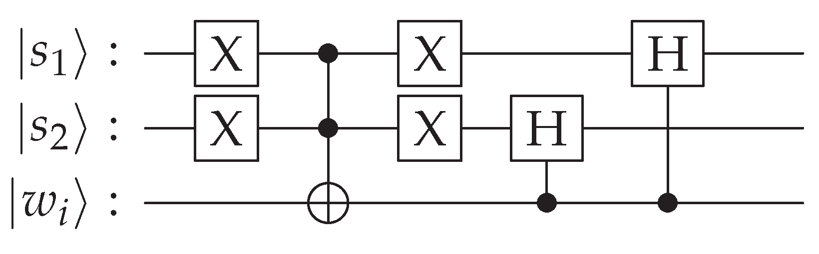
where spans the desired subspace and corresponds to the unwanted all-zero component. Applying the operation depicted in Figure A2 to s and w affects only the component, transforming it into , where
In general, the i-th application of the operation on s and w affects only , transforming it into , where
and the first i qubits of w are in the state 1. After L applications of this operation, the joint state of s and w can be expressed as:
The amplitude of is , so the residual weight of the unwanted all-zero component is , i.e., exponentially small in L. Within each branch i, the k desired basis states carry equal amplitudes (i.e., for the present case , ), so the marginal distribution over the desired basis states is uniform up to the residual weight that the state places on the unwanted component. Each application of the operation to the all-zero component of s requires one additional auxiliary qubit initialized to 0, so the register w comprises L qubits. Like s, the register w is retained as part of the branch label of its round [Equations (4) and (5)] and does not return to , so that each of the r rounds uses its own copy; choosing for a fixed keeps the residual weight of the unwanted all-zero component small enough that the total error accumulated over the rounds, of order , is .
The third case () requires a uniform superposition over a specified subset S of k of the computational basis states, which can be prepared exactly by standard state-preparation techniques. Starting from the equal superposition , the indicator function of S is computed into an auxiliary qubit and one step of amplitude amplification [20] rotates the marked component into the target state . Since the subset occupies a fraction of the search space, amplification iterations suffice, and the indicator of S is evaluated with elementary gates from its classical description; alternatively, the uniform superposition over can be prepared directly by the recursive construction of Ref. [22] and mapped onto S by a classically controlled permutation. In both cases the prepared state deviates from the exact uniform superposition by at most at a cost of gates, which leaves the exponential scaling of Equation (11) unaffected.
Conditional structure. The selection that defines each factor of Equation (3)—clauses true and clause false—is a computational-basis condition on the clause registers , and is therefore realized by a multiply-controlled gate: the m control patterns are computed simultaneously into a flag register by a reversible cascade of gates with work ancillas, is then applied controlled on the i-th flag, and the flags are uncomputed; if no flag is set, i.e., if every clause is satisfied, no expansion is applied. Because changes only the assignment and label registers, the clause registers are untouched while the expansion acts, so the flags remain valid and their uncomputation is exact, returning all work ancillas to 0 for reuse in the next round. The conditional structure thus adds gates per round to the gates of the clause evaluation, which leaves the polynomial overhead of Section 3.5 unchanged.
Figure A1.
Entanglement between computational basis components of s and a via four Toffoli gates. The first gate entangles the 11 component of s with the 0001 component of a; the second, third, and fourth gates analogously entangle 10, 00, and 01 of s with 0010, 1000, and 0100 of a, respectively.
Figure A1.
Entanglement between computational basis components of s and a via four Toffoli gates. The first gate entangles the 11 component of s with the 0001 component of a; the second, third, and fourth gates analogously entangle 10, 00, and 01 of s with 0010, 1000, and 0100 of a, respectively.
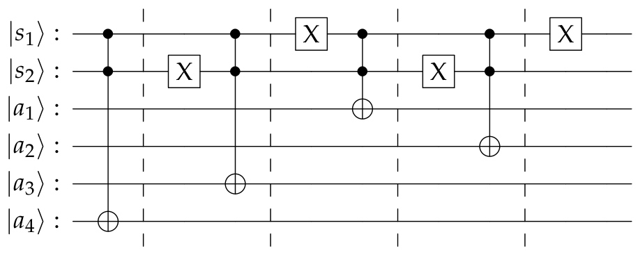
Figure A2.
Circuit decomposition of the expansion operation on the all-zero component of s using an ancilla qubit .
Figure A2.
Circuit decomposition of the expansion operation on the all-zero component of s using an ancilla qubit .
References
- Karp, R.M. Reducibility Among Combinatorial Problems. In 50 Years of Integer Programming 1958-2008: From the Early Years to the State-of-the-Art; Jünger, M., Liebling, T.M., Naddef, D., Nemhauser, G.L., Pulleyblank, W.R., Reinelt, G., Rinaldi, G., Wolsey, L.A., Eds.; Springer Berlin Heidelberg: Berlin, Heidelberg, 2010; pp. 219–241. [Google Scholar] [CrossRef]
- Paturi, R.; Pudlák, P.; Zane, F. Satisfiability Coding Lemma. In Proceedings of the Proceedings of the 38th Annual IEEE Symposium on Foundations of Computer Science (FOCS ’97), 1997; pp. 566–574. [Google Scholar] [CrossRef]
- Schöning, U. A probabilistic algorithm for k-SAT and constraint satisfaction problems. In Proceedings of the Proceedings of the 40th Annual IEEE Symposium on Foundations of Computer Science (FOCS ’99), 1999; pp. 410–414. [Google Scholar] [CrossRef]
- Brueggemann, T.; Kern, W. An improved deterministic local search algorithm for 3-SAT. Theor. Comput. Sci. 2004, 329, 303–313. [Google Scholar] [CrossRef]
- Hofmeister, T.; Schöning, U.; Schuler, R.; Watanabe, O. A Probabilistic 3-SAT Algorithm Further Improved. In Proceedings of the Proceedings of the 19th Annual Symposium on Theoretical Aspects of Computer Science, Berlin, Heidelberg, 2002; STACS ’02, pp. 192–202. [Google Scholar]
- Paturi, R.; Pudlák, P.; Saks, M.E.; Zane, F. An improved exponential-time algorithm for k-SAT. J. ACM 2005, 52, 337–364. [Google Scholar] [CrossRef]
- Hertli, T. 3-SAT Faster and Simpler—Unique-SAT Bounds for PPSZ Hold in General. SIAM J. Comput. 2014, 43, 718–729. [Google Scholar] [CrossRef]
- Hansen, T.D.; Kaplan, H.; Zamir, O.; Zwick, U. Faster k-SAT algorithms using biased-PPSZ. In Proceedings of the Proceedings of the 51st Annual ACM SIGACT Symposium on Theory of Computing (STOC ’19), 2019; pp. 578–589. [Google Scholar] [CrossRef]
- Dantsin, E.; Goerdt, A.; Hirsch, E.A.; Kannan, R.; Kleinberg, J.; Papadimitriou, C.; Raghavan, P.; Schöning, U. A deterministic (2-2/(k+1))n algorithm for k-SAT based on local search. Theor. Comput. Sci. 2002, 289, 69–83. [Google Scholar] [CrossRef]
- Moser, R.A.; Scheder, D. A Full Derandomization of Schöning’s k-SAT Algorithm. In Proceedings of the Proceedings of the 43rd Annual ACM Symposium on Theory of Computing (STOC ’11), 2011; pp. 245–252. [Google Scholar]
- Scheder, D. Guided Search and a Faster Deterministic Algorithm for 3-SAT. In Proceedings of the LATIN 2008: Theoretical Informatics; Laber, E.S., Bornstein, C., Nogueira, L.T., Faria, L., Eds.; Berlin, Heidelberg, 2008; pp. 60–71. [Google Scholar]
- Kutzkov, K.; Scheder, D. Using CSP To Improve Deterministic 3-SAT. arXiv 2010, arXiv:1007.1166. [Google Scholar]
- Shor, P.W. Polynomial-Time Algorithms for Prime Factorization and Discrete Logarithms on a Quantum Computer. SIAM J. Comput. 1997, 26, 1484–1509. [Google Scholar] [CrossRef]
- Grover, L.K. Quantum Mechanics Helps in Searching for a Needle in a Haystack. Phys. Rev. Lett. 1997, 79, 325–328. [Google Scholar] [CrossRef]
- Shenvi, N.; Kempe, J.; Whaley, K.B. Quantum random-walk search algorithm. Phys. Rev. A 2003, 67, 052307. [Google Scholar] [CrossRef]
- Schuld, M.; Sinayskiy, I.; Petruccione, F. An introduction to quantum machine learning. Contemp. Phys. 2015, 56, 172–185. [Google Scholar] [CrossRef]
- Biamonte, J.; Wittek, P.; Pancotti, N.; Rebentrost, P.; Wiebe, N.; Lloyd, S. Quantum machine learning. Nature 2017, 549, 195–202. [Google Scholar] [CrossRef] [PubMed]
- Gemeinhardt, F.; Garmendia, A.; Wimmer, M.; Weder, B.; Leymann, F. Quantum Combinatorial Optimization in the NISQ Era: A Systematic Mapping Study. ACM Comput. Surv. 2024, 56, 36. [Google Scholar] [CrossRef]
- Ambainis, A. Quantum search algorithms. ACM SIGACT News 2004, 35, 22–35. [Google Scholar] [CrossRef]
- Brassard, G.; Høyer, P.; Mosca, M.; Tapp, A. Quantum amplitude amplification and estimation. Contemp. Math. 2002, arXiv:quant305, 53–74. [Google Scholar] [CrossRef]
- Brehm, M.; Weggemans, J. Assessing fault-tolerant quantum advantage for k-SAT with structure. Quantum 2026 1975, arXiv:2412.1327410. [Google Scholar] [CrossRef]
- Grover, L.; Rudolph, T. Creating superpositions that correspond to efficiently integrable probability distributions. arXiv 2002. [Google Scholar]
Figure 1.
Quantum circuit implementing procedure F. The qubit encodes the quantum truth value of the i-th clause; the block is activated only when (open circle, i.e., clause is false) while all preceding clauses are true (filled circles), so that at most one block acts on each computational basis state, and no block acts when every clause is satisfied (the filled control drawn on the row of dots belongs to the control line coming from the preceding clause qubits and passes through the omitted rows); s denotes the label register of the round, shared by its blocks , prepared in a uniform superposition of k basis states and retained as the branch label [Equations (4) and (5)] (each round uses its own copies of the clause registers and its own register ); and denotes the state of the round being expanded, i.e., the problem-dependent superposition constructed so far.
Figure 1.
Quantum circuit implementing procedure F. The qubit encodes the quantum truth value of the i-th clause; the block is activated only when (open circle, i.e., clause is false) while all preceding clauses are true (filled circles), so that at most one block acts on each computational basis state, and no block acts when every clause is satisfied (the filled control drawn on the row of dots belongs to the control line coming from the preceding clause qubits and passes through the omitted rows); s denotes the label register of the round, shared by its blocks , prepared in a uniform superposition of k basis states and retained as the branch label [Equations (4) and (5)] (each round uses its own copies of the clause registers and its own register ); and denotes the state of the round being expanded, i.e., the problem-dependent superposition constructed so far.
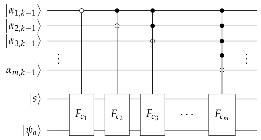
Figure 2.
Verification of the two bounds entering the exponent, for . (a) The measured in units of the entropy factor , for , , , , and . Solid lines are the exact binomial tail with r the integer nearest , open symbols the Monte Carlo estimate at the same points, dotted lines the lower bound of Equation (10) and the dashed line its upper bound; every value lies inside the window. (b) The measured marked amplitude in units of the guaranteed bound , drawn as the dashed line at unity, for the radii of panel (a) and for the optimal radius up to . The bound holds everywhere and is increasingly conservative as r grows.
Figure 2.
Verification of the two bounds entering the exponent, for . (a) The measured in units of the entropy factor , for , , , , and . Solid lines are the exact binomial tail with r the integer nearest , open symbols the Monte Carlo estimate at the same points, dotted lines the lower bound of Equation (10) and the dashed line its upper bound; every value lies inside the window. (b) The measured marked amplitude in units of the guaranteed bound , drawn as the dashed line at unity, for the radii of panel (a) and for the optimal radius up to . The bound holds everywhere and is increasingly conservative as r grows.
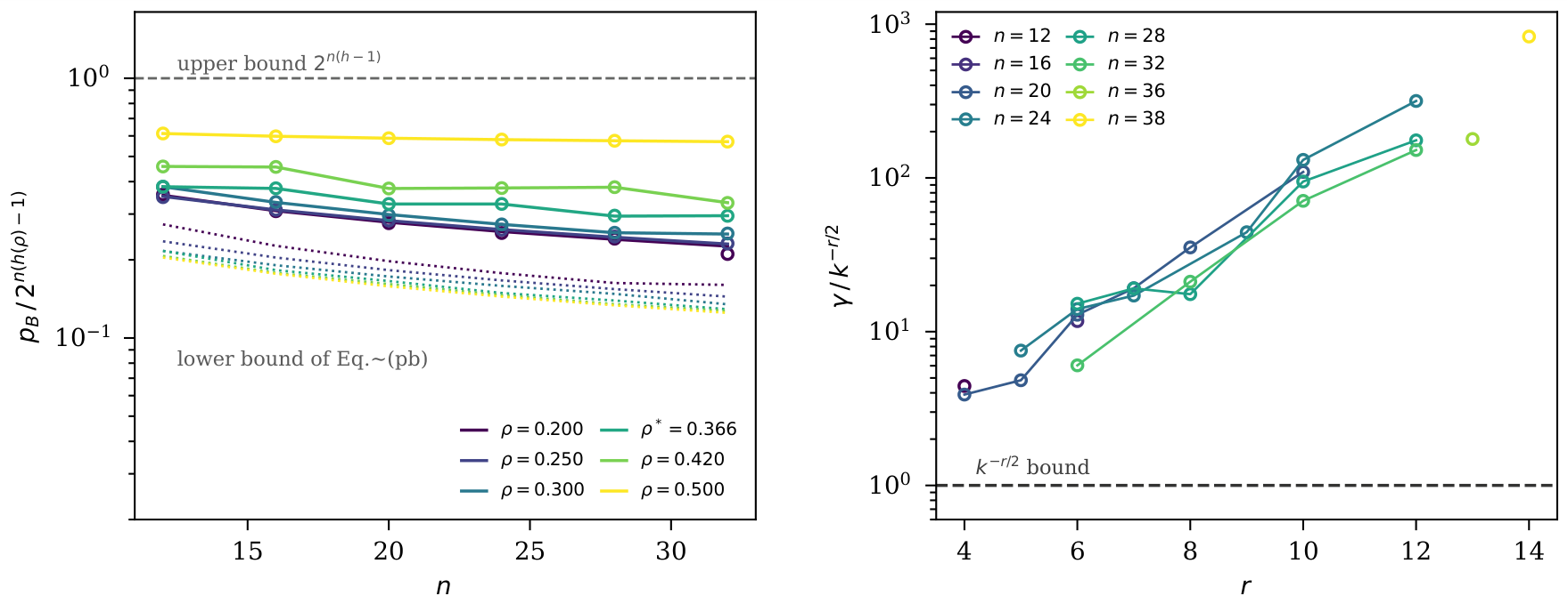
Figure 3.
Total cost at the optimal radius against n, for . Symbols are the measured values of Table 4, the solid line a least-squares fit over and the dashed line the asymptotic bound of Equation (11). The measured base lies below the bound because the bound uses the worst-case amplitude , and over this range of n the polynomial overheads that Equation (11) discards are of the same order as the difference.
Figure 3.
Total cost at the optimal radius against n, for . Symbols are the measured values of Table 4, the solid line a least-squares fit over and the dashed line the asymptotic bound of Equation (11). The measured base lies below the bound because the bound uses the worst-case amplitude , and over this range of n the polynomial overheads that Equation (11) discards are of the same order as the difference.
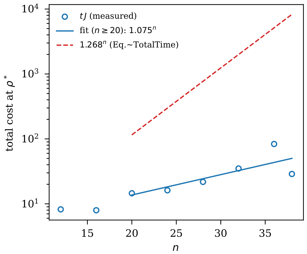

Table 1.
Resources of the proposed algorithm at the optimal radius , for . Classically repeated runs: , with h the binary entropy function. Amplitude-amplification iterations per run: . Exponential base of Equations (11) and (12): , so that up to polynomial factors.
| k | t | Iterations | ||
|---|---|---|---|---|
| 3 | ||||
| 4 | ||||
| 5 |
Table 2.
Exponential base in the gate-model running time for worst-case 3-SAT. The first two rows are classical reference points included for comparison; the remaining rows are quantum gate-model algorithms.
Table 2.
Exponential base in the gate-model running time for worst-case 3-SAT. The first two rows are classical reference points included for comparison; the remaining rows are quantum gate-model algorithms.
| Algorithm | Base |
|---|---|
| Classical: Schöning’s local search [3] | |
| Classical: best known (PPSZ-type) [6,7,8] | |
| Grover search (oracle only) [14] | |
| Grover search + Hofmeister et al. [5,19] | |
| Amplitude amplification + PPSZ [6,8,20] | |
| This work (Grover within a Hamming ball, hybrid) |
Table 3.
Exponential bases in the running time for general k: Schöning’s local search [3], the deterministic Hamming-ball template [9], and the exponent obtained here. The present exponent lies below both classical bounds for every .
| k | Schöning | Hamming ball | This work |
|---|---|---|---|
| 3 | |||
| 4 | |||
| 5 | |||
| 6 | |||
| 7 | |||
| 8 | |||
| 9 | |||
| 10 |
Table 4.
Numerical verification at the optimal radius for . is the exact binomial tail ; is the marked amplitude of Equation (13) measured by exact enumeration of the branch tree; and is the base of the total cost , with classically repeated balls of amplitude-amplification iterations each, to be compared with of Equation (11). The guaranteed lower bound is .
Table 4.
Numerical verification at the optimal radius for . is the exact binomial tail ; is the marked amplitude of Equation (13) measured by exact enumeration of the branch tree; and is the base of the total cost , with classically repeated balls of amplitude-amplification iterations each, to be compared with of Equation (11). The guaranteed lower bound is .
| n | r | ||||
|---|---|---|---|---|---|
| 12 | 4 | ||||
| 16 | 6 | ||||
| 20 | 7 | ||||
| 24 | 9 | ||||
| 28 | 10 | ||||
| 32 | 12 | 152 | |||
| 36 | 13 | 179 | |||
| 38 | 14 | 831 |
Disclaimer/Publisher’s Note: The statements, opinions and data contained in all publications are solely those of the individual author(s) and contributor(s) and not of MDPI and/or the editor(s). MDPI and/or the editor(s) disclaim responsibility for any injury to people or property resulting from any ideas, methods, instructions or products referred to in the content. |
© 2026 by the authors. Licensee MDPI, Basel, Switzerland. This article is an open access article distributed under the terms and conditions of the Creative Commons Attribution (CC BY) license (http://creativecommons.org/licenses/by/4.0/).
Copyright: This open access article is published under a Creative Commons CC BY 4.0 license, which permit the free download, distribution, and reuse, provided that the author and preprint are cited in any reuse.