

Submitted:
16 September 2026
Posted:
16 September 2026
You are already at the latest version
Abstract
Probabilistic machine-learning outputs are increasingly used in financial decision-support systems, yet small or unstable score differences can trigger costly portfolio changes. We develop a two-stage machine-learning decision-support framework for a fixed-size exchange-traded fund (ETF) portfolio. Frozen model scores undergo non-decreasing logistic recalibration on an independent Calibration stage. A zero-slope optimum closes the calibration gate and prohibits discretionary membership replacement; positive-slope groups proceed to Policy Validation, which selects a candidate–holding margin boundary or no active updating. The audit-triggered corrected evaluation covers 18 Chinese equity ETFs, three model classes, and seven non-overlapping evaluation periods. Brier score decreased in 15 of 21 model–period groups, although the mean Monotone-minus-RAW Brier change remained near zero (0.000079); expected calibration error decreased in 17 groups and grouped reliability error in 19. Nine fits retained positive slopes and 12 reached the zero boundary. Among the two prespecified primary models, seven of 14 groups closed at Calibration, five further groups selected no active updating, and two authorized updating. Relative to uncalibrated model probabilities (RAW), monotone paths reduced active replacements from 26 to 11, active-member turnover from 6.50 to 2.75, and mean transaction cost from 25.20 to 19.35 basis points of initial equity. The seven-window economic contrast was positive in two windows, negative in three, and zero in two (mean 0.005187). The framework authorizes or refuses unsupported actions without claiming return enhancement.
Keywords:
machine learning
; financial technology (FinTech)
; probability recalibration
; decision support
; abstention
; exchange-traded funds
; portfolio updating
; turnover constraint
1. Introduction
Exchange-traded funds (ETFs) provide liquid, low-cost access to diversified market exposures, and machine learning is increasingly used to rank assets and support systematic portfolio updating. A common workflow fits a predictive model, ranks the available assets, and reconstructs a Top-K portfolio at each rebalancing date. This workflow can extract nonlinear cross-sectional information, but it can also turn small and unstable score changes into repeated trades. The practical research problem is therefore not only whether a model predicts well, but whether its output provides sufficient evidence to justify a costly portfolio change [1,2,3,4,5,6,7].
Existing approaches mainly improve the predictor, calibrate its probabilities, impose turnover constraints, or apply confidence and no-trade thresholds. These methods address important parts of the deployment problem, yet three gaps remain when a fixed-size portfolio is updated recursively. Raw probabilities may not correspond to observed event frequencies; an absolute confidence threshold does not compare a candidate with the asset it would replace; and ranking changes do not by themselves establish that turnover and transaction costs are economically justified [8,9,10,11,12,13].
These gaps motivate a decision interface centered on portfolio-relative evidence. In the present application, the probability difference between a candidate ETF and a current holding is interpreted as evidence for replacement. The probability map must therefore be non-decreasing: a decreasing recalibration would reverse the frozen score ordering and contradict the meaning of the candidate–holding margin. The deployment decision must then separate whether Calibration retains a positive score–outcome direction, whether independent Policy Validation authorizes a finite action boundary, and whether the resulting account path produces economic value after costs. Recent calibration research similarly treats monotonicity or ranking preservation as an explicit design property [14,15].
This article develops a cost-sensitive two-stage authorization protocol around these requirements. Frozen base models provide native scores, and a constrained non-decreasing logistic map adjusts their probability scale. A zero fitted slope closes the Calibration gate and prohibits discretionary membership replacement; positive-slope groups proceed to Policy Validation, which selects either a finite candidate–holding boundary or no active updating. A common recursive account engine then enforces the fixed portfolio size, one-replacement budget, next-day execution, equal-weight restoration, and transaction-cost accounting. Accordingly, the ETF setting serves as a FinTech application of a broader machine-learning decision-support problem: how probabilistic outputs should be translated into costly sequential actions when the system is allowed to abstain.
The study addresses four research questions. RQ1 asks how monotone score-space logistic recalibration changes held-out probability quality. RQ2 asks how often the constrained fit retains a positive score–outcome association and how often it activates calibration-stage abstention. RQ3 characterizes how final monotone-gated policies alter authorization coverage, discretionary replacements, turnover, and costs relative to corresponding uncalibrated model-probability (RAW) policies. RQ4 evaluates whether these changes translate into incremental held-out economic value.
The contribution is an integrated deployment protocol rather than a new general-purpose calibration algorithm. First, it turns calibrated probabilities into portfolio-relative candidate–holding evidence while preserving the ordering semantics needed by the replacement decision. Second, it connects calibration-stage abstention, independently validated action authorization, and a common recursive account so that probability quality, realized activity, costs, and economic outcomes can be evaluated along one auditable chain. The reported evidence is intentionally bounded: reliability improves more consistently than total probabilistic loss, two-stage abstention limits realized activity, and economic effects remain heterogeneous.
2. Related Work
2.1. Machine Learning, FinTech, and Portfolio Implementation
Cross-sectional asset-prediction research uses linear and regularized models, tree-based learners, and deep architectures to capture nonlinear interactions and high-dimensional predictors [1,2,3,4]. Evidence from the Chinese stock market further shows that apparent predictive performance depends on market structure, sample construction, and evaluation design [5]. Much of this literature ranks assets and evaluates portfolio outcomes after prediction. The translation from a small score change to a membership replacement is often treated as part of portfolio construction rather than as a separately validated decision.
Flexible predictors can therefore create unstable portfolio changes even when their average forecasting performance is competitive. Transaction costs and turnover restrictions become first-order implementation considerations [7,13]. Equal weighting is useful when the objective is to isolate membership decisions rather than combine them with continuous weight estimation [16]. The remaining gap is a transparent rule for deciding when the relative evidence between a candidate and a current holding is strong enough to authorize replacement.
Predict-then-optimize and decision-focused-learning research emphasizes that prediction metrics need not align with downstream constrained decisions [17,18]. The present framework does not train a portfolio objective end to end. Instead, it separates base-model fitting, probability recalibration, policy selection, and account evaluation so that each layer remains auditable.
2.2. Probability Calibration and Ranking Preservation
The Brier score measures squared error between predicted probabilities and binary outcomes, with lower values indicating better probabilistic forecasts [19,20]. Its classical decomposition separates reliability, which measures probability–frequency agreement; resolution, which reflects separation between groups with different observed outcome frequencies; and uncertainty, which is determined by the overall event rate [21]. Logistic post-hoc calibration is widely used to convert an uncalibrated scalar score into a probability [22,23]. Calibration error, however, depends on the estimator and binning design, so no single diagnostic should be treated as sufficient [10,24].
For decisions based on pairwise probability differences, ordering is part of the method definition. Receiver operating characteristic (ROC)-regularized and constrained monotonic calibration methods explicitly recognize the value of preserving ranking while adjusting probability reliability [14,15]. Our two-parameter logistic map is simpler than those general methods: it is imposed as a non-decreasing score-to-probability interface because a decreasing map would reverse the candidate–holding interpretation.
2.3. Selective Action, Abstention, and No-Trade Policies
Selective prediction permits a system to abstain instead of forcing a prediction or action for every observation [11,25]. Financial threshold rules apply a related idea by requiring stronger evidence before executing a trade [12]. Portfolio research also recognizes no-trade regions and economically constrained policies as tools for limiting unnecessary turnover [7,13].
Our framework differs in the location and meaning of abstention. A zero constrained recalibration slope closes the calibration gate because a constant probability contains no candidate–holding evidence. For positive slopes, a separate Policy Validation stage can still select no active updating. These are two distinct abstention decisions: one concerns the direction supported by Calibration, and the other concerns the action boundary supported by validation utility.
The distinction is also one of component integration. Calibration studies primarily target probabilistic reliability, selective-prediction studies usually abstain at the prediction level, and financial no-trade rules typically constrain an already formed trading signal. This study connects these layers through a portfolio-relative margin, a non-decreasing score-to-probability interface, a separately validated action boundary, and a common recursive account engine. The contribution is therefore an auditable decision protocol that clarifies where abstention occurs and how it propagates to execution and cost attribution, rather than a claim that any individual component is novel in isolation.
Table 1 makes this integration claim explicit. It is a component map of the representative literature streams cited above, not a claim that every paper in a stream lacks every unmarked element. The novelty claimed here is the stage-defined combination and audit linkage of the components, rather than invention of calibration, abstention, or turnover control individually.
3. Materials and Methods
3.1. Notation and Stage Linkage
To reduce visual clutter, the formal definitions use local notation. Unless a comparison across groups requires otherwise, we condition on a fixed base model a and rolling window w and suppress the indices . ETF identifiers are indexed by i and j, rebalancing dates by t, probability states by , candidate–holding pairs by q, ten-day return periods by u, evaluation observations by , and calibration bins by b. Full group indices are restored in result-level comparisons and audit artifacts. Certainty-equivalent return (CER) is the account-level economic criterion used below. Figure 1 provides the semantic overview of the stage linkage; after the component quantities have been defined, Equation (17) gives the corresponding compact mathematical summary.
3.2. Study Design and Temporal Protocol
The study uses a pre-specified ETF panel and seven rolling windows. Each window separates Training, Calibration, Policy Validation, and a previously held-out evaluation period; a purge removes observations whose label endpoints cross the next-stage boundary. The model, recalibration map, policy boundary, and account rules are fitted or selected only in their authorized stages. The empirical panel composition and exact window boundaries are reported with the experimental setting in Section 4.1 and in Supplementary Tables S1 and S2. Figure 1 summarizes the complete stage-separated workflow, including the RAW and monotone branches, the Calibration gate, Policy Validation, and the common recursive account engine.
To make the source of researcher degrees of freedom explicit, Table 2 records the principal frozen design choices and the stage in which they are used. These values are frozen protocol inputs that were unchanged by the audit-triggered correction; they are not quantities selected from the corrected held-out outcomes.
3.2.1. Point-in-Time Universe, Labels, and Features
The local-index convention introduced above is used throughout the formal definitions, with the model–window pair understood unless it is written explicitly. Let be the set of eligible ETFs on signal date t. For , let be the first eligible trading day after t, and let be the tenth eligible trading day after . The back-adjusted (HFQ) price series is used for label construction. The label return is
where and are respectively the back-adjusted opening and closing prices used only to construct the forward label. The account layer separately uses unadjusted market prices for execution and valuation. Let be the descending cross-sectional rank of , with rank one assigned to the largest return. Let denote the indicator function, equal to one when its argument is true and zero otherwise. Define
Thus is the number of positive labels on date t, and identifies membership in the future top 30% of the eligible cross-section. The signal-date universe is fixed before any forward outcome is inspected. If any eligible ETF lacks a required endpoint, the date is marked LABEL_DATE_INVALID and the entire date is excluded; individual ETFs are never deleted to restore a cross-section after observing future data. The feature vector contains only information available through t, whereas is assigned only after the forward endpoint is known.
The feature vector contains 13 price–volume characteristics computed only from date t and earlier observations: 5- and 20-day momentum, short reversal, 10-day moving-average deviation, 20-day volatility, 14-day relative strength index, moving-average-convergence–divergence, 10-day high–low range, 20-day maximum drawdown, 5-day volume change, 20-day Amihud illiquidity, and 20-day return skewness and kurtosis. The two momentum variables measure directional persistence at short and medium horizons; short reversal measures one-day mean reversion; moving-average deviation, relative strength, and moving-average convergence–divergence describe trend position and overextension; volatility, high–low range, and maximum drawdown represent dispersion, intraday range, and downside history; volume change and Amihud illiquidity describe trading activity and liquidity; and skewness and kurtosis represent distributional asymmetry and tail concentration. Median imputation and standardization are fitted inside each Training fold. The processed is the sole predictor input used to estimate the local score , while is its binary Training target; no forward return enters . Complete equations and minimum histories appear in Supplementary Table S3; the frozen model grids and fitting details appear in Supplementary Table S4.
3.3. Base Models and Monotone Recalibration
Model index , , and denotes standard logistic regression, elastic-net logistic regression, and LightGBM, respectively [26,27]. Standard logistic regression serves as a low-complexity policy baseline, whereas elastic-net logistic regression and LightGBM are the two prespecified primary policy models. Hyperparameters are selected entirely inside Training by three chronological folds, with fitting rows and label endpoints restricted to dates before the fold validation start. Mean binary log loss is the selection criterion, with lower values indicating better probabilistic fit. Preprocessing is fitted separately inside each fold. Here, denotes inverse regularization strength, the -ratio controls the relative contribution of and penalties in the elastic-net model, and the maximum number of leaves controls LightGBM tree complexity. The frozen grids are for standard logistic regression; and -ratio for elastic-net logistic regression; and leaves , learning rate 0.05, and 60 trees for LightGBM. No class weights or resampling are used.
For the fixed model–window pair, let be the frozen native positive-class score for ETF i on date t, where the positive class is future membership in the top 30% of the eligible cross-section defined in Equation (2). The RAW probability is
For logistic models, is the real-valued linear decision score before the sigmoid transformation; for LightGBM, it is the corresponding binary raw margin. A read-only audit verified agreement between Equation (3) and the stored positive-class probability to machine precision for all 21 model–window groups.
3.3.1. Constrained Recalibration and Calibration Gate
Let denote the ETF–date observations assigned to Calibration in the fixed window. The intercept is unrestricted, whereas the slope is constrained to be non-negative so that recalibration cannot reverse the ordering induced by the frozen score. For arbitrary , define
The fitted parameters are obtained by minimizing Calibration log loss under the same non-negativity constraint:
The reported Monotone probability is . The two-parameter objective is convex. This constrained logistic map was chosen for its convex objective, interpretable direction, exact Karush–Kuhn–Tucker (KKT) zero-boundary state, and limited flexibility under the relatively small Calibration samples. The optimizer permits the exact boundary solution ; boundary status is confirmed by the KKT condition rather than by a tuned positive-slope threshold. The KKT check establishes that is the constrained optimum rather than a small positive estimate classified as zero by an arbitrary decision threshold. A numerical reporting tolerance is used only to identify the optimizer’s recorded boundary state and is not varied as a model parameter.
The Calibration gate is represented by a binary variable g: admits the Monotone state to Policy Validation, whereas closes the gate. Using the indicator function defined above,
When , Equation (4) is strictly increasing and preserves the frozen score ordering. When , all monotone probabilities equal . The zero-gate state is therefore a statement about the current constrained recalibration fit, not a universal rejection of the base predictor. Let denote the held-out decision dates. The discretionary replacement set is then empty throughout held-out evaluation:
This deterministic no-active-update rule prevents security-code tie-breaking from producing arbitrary membership changes under constant probabilities. It is a decision-interface rule introduced in this study, not a general claim that the base model has no predictive ability.
3.4. Two-Stage Action Authorization and Recursive Account
Let be the four ETFs held immediately before the discretionary decision on date t, after any forced event has been processed, with . The candidate set is . For a candidate , holding , and probability state , define
The margin is relative evidence for replacing holding i with candidate j; it is not a cardinal expected-return difference. For example, means that the candidate probability exceeds the holding probability by five percentage points; it does not represent a 5% expected-return advantage. At fixed within the current model–window pair, let order by decreasing probability, and let order by increasing probability. Ties are resolved by the frozen ETF code order. The paired margins are
At most discretionary membership replacement is allowed per rebalancing date; consequently, only can be authorized in this study.
The finite boundary set is
The boundary is measured on the probability scale; for example, requires a four-percentage-point candidate advantage before discretionary replacement can be authorized. We use NAU to denote no active update and write the corresponding policy as . RAW policies always enter Policy Validation. A monotone policy enters Policy Validation only when . For a finite , let denote the unadjusted opening price used for next-day execution, and let denote execution feasibility of pair q on date t. The value requires valid positive execution prices for the outgoing and incoming ETFs, a sellable outgoing ETF, and a buyable incoming ETF. The authorized discretionary action set is
Thus is either the single best candidate–holding pair or the empty set, and is the number of authorized discretionary replacements. A policy is eligible only if its annualized one-way active-member turnover is at most 2.4. Let be the Policy Validation rebalancing dates and T the number of trading days in that stage. Define
where is annualized active-member turnover, not realized capital turnover; forced events do not enter it. Define and . Policy Validation evaluates net certainty-equivalent return (CER) at the prespecified primary risk-aversion coefficient ; the account-level CER definition is given explicitly below. Let be the set of eligible boundaries attaining the best validation CER. The maximizing set and the frozen tie choice are
The second line of Equation (13) implements the frozen tie rule: among CER values equal within the recorded numerical tolerance, the largest boundary is selected, and denotes no active updating. RAW and open-gate Monotone states select their policies separately because recalibration changes the numerical probability scale. A closed Monotone gate bypasses this selection and sets before entering the common account engine.
3.4.1. Recursive Account, Execution, and Costs
Signals are formed at the close and executed at on the next trading day. A security with zero volume or an invalid is not tradable. Buy-side and sell-side commission plus comprehensive trading fees are 0.0005 per notional, and slippage is 0.0005 per notional on each side. ETF secondary-market stamp tax is zero; no minimum commission is modeled. Initial equity is 1,000,000 monetary units per account path. RAW and monotone paths share the same cash-funded RAW-probability Top-K initial holdings within each model–window pair. This common RAW-ranked initialization isolates subsequent action authorization: positive-slope monotone mappings preserve the same initial ordering, whereas zero-slope mappings contain no defensible ranking and would otherwise require arbitrary tie-breaking. Portfolios are long only and restored to equal weights after execution. The account applies the retained dividend and share-adjustment ledger identically to both methods; the final audit contains 20 applied dividends and 11 applied share adjustments.
The policy equations describe discretionary membership authorization only. To define the account state, let be cash immediately after the transition on date t, let be the number of shares of ETF i, and let be its unadjusted valuation price. Then
Thus is total equity and is the post-transition portfolio weight. The superscript denotes the account state immediately before the transition at date t. The deterministic account transition applies valid sell orders before buy orders, exact cash feasibility, order-specific costs, retained dividends, share adjustments, and equal-weight restoration, where is the pre-specified ledger of execution feasibility and corporate-action events on date t. Consequently, a closed gate or uses the same map with ; it disables discretionary replacement but not valuation, forced events, or corporate actions.
For a fixed selected account path, let be the net portfolio return in ten-trading-day period u and let N be the number of periods. Define
where is the arithmetic mean and is the second central moment, i.e., the population-form variance of the observed net ten-day return series. Certainty-equivalent return rewards a higher mean net return while penalizing return variability; higher values are preferred. For risk-aversion coefficient , annualized net certainty-equivalent return is
The factor converts ten-trading-day moments to an annual scale. The primary value is ; is a prespecified sensitivity analysis reported in Supplementary Table S11.
With all component quantities now defined, the stage-wise decision chain can be summarized compactly. For this summary, admits every RAW state to Policy Validation and applies the Calibration gate:
This expression is a compact summary rather than an additional decision rule: Training fixes f, Calibration estimates and determines monotone eligibility, Policy Validation selects , and held-out evaluation applies the frozen action and account maps without refitting.
The objectives are deliberately stage-specific rather than interchangeable. Training log loss selects the base probabilistic model; Calibration log loss fits the low-dimensional constrained probability map; Policy Validation maximizes net CER subject to the turnover-eligibility rule; and held-out evaluation reports probability quality and realized account outcomes without feeding them back into any earlier stage of the corrected replay. Brier score is the primary held-out probability-quality metric, while ECE, reliability decomposition, calibration slope/intercept diagnostics, realized activity, costs, and CER answer different diagnostic or economic questions. This stage-local separation does not erase the audit history described below: the monotone correction itself was registered after the original held-out outputs had been viewed. Table 3 summarizes the information flow within the corrected replay.
3.5. Evaluation and Audit Protocol
For a fixed model–window group and probability state, let be the evaluation ETF–date observations, with and . The Brier score (BS) is the mean squared error of the probabilistic forecasts; lower values indicate better probabilistic accuracy. It is defined as
Expected calibration error (ECE) is the secondary calibration diagnostic. It summarizes the weighted discrepancy between average predicted probabilities and observed event frequencies across bins; lower values indicate better calibration. All probability changes use the convention
so a negative value denotes improvement. Expected calibration error uses ten equal-width bins. Let for , with , let , and define and for nonempty bins. Then
Brier score is the primary probability metric; ECE, calibration intercept and slope, reliability diagrams, and a grouped ten-bin Brier decomposition are diagnostic. With , write reliability, resolution, and uncertainty as , , and , respectively. The grouped decomposition is
where
Lower reliability error and higher resolution are favorable. Because the diagnostic uses fixed bins, its resolution term reflects bin occupancy and must not be interpreted as a direct change in ranking discrimination for positive-slope mappings.
RQ3 characterizes how the final monotone-gated policies alter authorization coverage, discretionary replacements, turnover, and costs relative to the corresponding RAW policies. RQ4 uses the paired Monotone-minus-RAW contrast as its primary economic estimand because RAW and Monotone share the same frozen base model, initialization, execution rules, account engine, and cost semantics within each model–window pair. This matched counterfactual isolates the incremental effect of the recalibration-and-authorization interface; it is not designed as a claim of market-beating performance. The comparison is averaged across the two primary policy models within each of the seven non-overlapping held-out periods. The seven windows are the primary descriptive unit; they are not treated as statistically independent replicates.
3.5.1. Audit-Triggered Correction and Reporting Status
A pre-submission semantic audit found that the original unconstrained logistic remapping of RAW probabilities could reverse the ordering produced by the frozen base model. Such reversals were inconsistent with candidate–holding margins as relative replacement evidence. All outputs dependent on the original remapping were therefore invalidated. Before recomputation, a single correction was registered: non-decreasing logistic recalibration of frozen native scores, KKT recognition of a zero-slope boundary, and deterministic no active updating when that boundary was reached. The ETF panel, data partitions, features, labels, fitted base models, RAW predictions, policy grid, account rules, transaction costs, and statistical definitions were unchanged. A subsequent registered unified account replay regenerated both RAW and monotone account paths under the corrected cash-funded initialization and common corporate-action, cost, tax, and CER semantics. The evaluation reported below is the sole authoritative audit-triggered corrected held-out result set; immutable prior outputs and the complete audit history are retained outside the inferential path.
4. Results
The Results are organized in the same order as the four research questions. Section 4.1 first establishes the empirical setting and audit integrity; the following sections then evaluate probability quality (RQ1), Calibration-gate states (RQ2), realized action authorization and costs (RQ3), and held-out economic effects (RQ4).
4.1. Empirical Setting and Protocol Integrity
The formal universe contains 18 surviving Chinese equity ETFs selected before the corrected evaluation. Products enter point in time only after their configured tradability and maturity requirements are met. The panel represents a pre-specified surviving set and does not reconstruct the complete historical Chinese ETF market. Back-adjusted (HFQ) histories are used for features and labels, whereas unadjusted prices are used for execution and valuation. All data were read from a frozen local AKShare cache, and no market data were downloaded during the corrected evaluation. The complete panel and entry metadata are provided in Supplementary Table S1.
Seven rolling windows isolate Training, Calibration, Policy Validation, and held-out evaluation. Their held-out periods do not overlap, although they share one market and rolling training histories; temporal dependence therefore cannot be excluded. Exact boundaries are shown in Table 4 and reproduced in Supplementary Table S2. The historical labels W03–W09 are retained verbatim from the frozen protocol and audit artifacts to preserve lineage; they identify the seven authorized complete windows and do not denote unreported held-out results.
The score-equivalence audit passed for all 21 model–window groups, with maximum numerical disagreement below . The constrained calibration fits produced nine positive interior slopes and 12 KKT zero-boundary solutions. The final replay registered 420 Policy Validation grid rows, 312 actual validation paths, and 42 final account paths: 21 RAW and 21 monotone. All fixed-portfolio ledger states satisfied , no forced maintenance events occurred, ETF stamp tax was zero, capital-conservation errors were zero, account artifacts were bound to the final authoritative manifest, and derived reporting artifacts were bound to a separate reporting manifest.
4.2. RQ1: Reliability Improved More Consistently Than Total Probabilistic Loss
Brier and grouped diagnostic summaries are reported in Table 5. Brier score decreased in 15 of 21 model–window groups, while ECE decreased in 17. Complete probability results and grouped decompositions are provided in Supplementary Tables S6 and S7; the corresponding visual summaries are shown in Figure 2 and Figure 3. Under the convention in Equation (19), the mean was and the median was . Thus, most groups showed small improvements, but a small number of larger deteriorations left the mean close to zero and slightly unfavorable. The mean was , and the median was .
The grouped Brier decomposition clarified the difference between ECE and total Brier loss. Reliability error decreased in 19 of 21 groups, but grouped resolution increased in only three. Among the nine positive-slope groups, Brier score, ECE, and reliability improved in seven, while grouped resolution increased in three. Among the 12 zero-boundary groups, reliability improved in all 12 and resolution increased in none. The zero-boundary maps collapse probabilities to a constant, explaining much of the grouped-resolution loss. Positive-slope maps preserve score ranking by construction; changes in grouped resolution for those groups reflect fixed-bin occupancy rather than a loss of ROC ordering.
4.3. RQ2: Half of the Policy Groups Entered Calibration-Stage Abstention
Across all probability groups, positive slopes were retained in 9 of 21 fits and the constrained optimum reached zero in 12. LightGBM retained positive slopes in five of seven periods, compared with two of seven for each logistic model (Table 6). Among the two prespecified primary policy models, seven of 14 groups opened the calibration gate and seven closed it.
Figure 4 visualizes the constrained recalibration slope and Calibration-gate state for each model–window group.
The gate states were consistent with the constrained objective rather than an additional performance screen. Positive boundary gradients at accompanied closed gates, whereas negative gradients led to positive interior slopes. The complete sample sizes, positive-label rates, score–label covariances, diagnostic AUC values, boundary gradients, and optimizer states are included in Supplementary Table S5 and visualized in Supplementary Figure S1. A zero slope is interpreted narrowly: under the current Calibration sample and constrained logistic map, the fit did not retain a positive score–outcome association. It is not interpreted as proof that the base model has no predictive ability in every period.
4.4. RQ3: Two-Stage Abstention Limited Realized Portfolio Activity
For the two prespecified primary policy models, 14 model–window groups followed four reporting pathways (Table 7). Seven groups closed at the Calibration gate. Of the seven positive-slope groups, five selected no active updating in Policy Validation and two selected finite boundaries that realized replacements in the held-out account. Thus, 12/14 primary groups abstained from discretionary membership replacement and 2/14 authorized it. Logistic regression is retained as a low-complexity exploratory policy baseline and is reported separately in the Supplementary Materials. These labels describe action authorization, not a claim that the account made no trades: initialization, equal-weight restoration, and corporate-action accounting remain active in all paths. The complete 21-group gate and policy-state summary is reported subsequently in Table 8.
Relative to the corresponding RAW final paths for the two primary policy models, monotone paths reduced active replacements from 26 to 11 and active-member turnover from 6.500 to 2.750 (Table 9). Mean transaction cost per primary-model path declined from 2520.27 to 1935.12 monetary units, equivalent to 25.20 versus 19.35 basis points of initial equity; the corresponding primary-path medians were 1852.13 versus 1598.63 monetary units, or 18.52 versus 15.99 basis points. Aggregate totals are descriptive sums across 14 primary-model paths. These reductions are consistent with lower discretionary updating and are partly mechanical consequences of lower action coverage; they do not alone establish superior economic utility. One final held-out path reached annualized active-member turnover of 2.50, exceeding the 2.40 eligibility level used in Policy Validation while satisfying the hard per-rebalancing budget . This is interpreted as imperfect validation-to-held-out transfer of aggregate activity, not as an account-rule violation. The complete three-model descriptive totals remain in the Supplementary Materials.
Across 350 paired held-out decision dates for the two primary policy models, both policies held on 317 dates, RAW replaced while monotone held on 22, RAW held while monotone replaced on seven, and both replaced on four. The hold-versus-replace disagreement rate was , with a tendency for the final monotone policy to suppress RAW-authorized replacements (Figure 5). The complete three-model action matrix contains 525 paired dates and is reported descriptively in the Supplementary Materials.
The final authoritative replay reports the selected RAW and monotone paths, not a new zero-boundary counterfactual for every open group. Superseded selected-versus-zero comparisons remain audit history and are not used for the main inference. This keeps the final economic comparison aligned with one account engine, one company-action ledger, zero ETF stamp tax, and the registered CER annualization.
4.5. RQ4: Economic Effects Were Heterogeneous
The window-level economic contrast is also visualized in Figure 6. The primary estimand is the equal average of the elastic-net logistic and LightGBM monotone-minus-RAW net differences within each of the seven windows. It was positive in two windows, negative in three, and zero in two; the mean difference was 0.005187. With seven temporally ordered windows, this is a descriptive effect summary rather than a formal independent-sample test. Across all 21 model–window pairs, the corresponding differences were positive in 6, negative in 5, and zero in 10. The complete values are reported in Table 10. The derived sensitivity analysis remained heterogeneous: the seven-window mean monotone-minus-RAW CER was -0.000206, 0.005187, and 0.010580 for , respectively; positive and negative window effects coexisted under all three settings.
W03 contributed the largest positive window-average difference, whereas W05 and W06 were negative. The corrected evaluation therefore does not establish a stable or statistically supported economic advantage of monotone over RAW policies.
5. Discussion
5.1. Interpretation of the Research Questions
RQ1 distinguishes probability reliability from total probabilistic loss. Most model–period groups showed lower ECE and grouped reliability error, but the average Brier change remained close to zero. Zero-boundary fits improved reliability by replacing heterogeneous scores with the Calibration base rate, while eliminating grouped resolution. Positive-slope fits preserved ranking, although fixed-bin resolution still changed with bin occupancy. Monotone recalibration therefore improved frequency alignment more consistently than it improved overall probabilistic loss.
RQ2 and RQ3 show that abstention occurred at two distinct decision layers. The Calibration gate asks whether the constrained score-to-probability relation retains a positive orientation; it is not a universal test of base-model validity. Policy Validation then asks whether an eligible candidate–holding margin supports active updating under the validation utility and turnover constraint. Twelve of 21 groups closed at Calibration, seven additional positive-slope groups selected no active updating, and two groups authorized finite-boundary updating and realized replacements. The resulting reduction in activity and costs supports the intended authorization mechanism, but lower turnover alone is not evidence of superior economic utility.
RQ4 confirms that economic value remained conditional. The primary seven-window contrast was positive in two windows, negative in three, and zero in two, with a mean of 0.005187. Across all 21 model–window pairs, 6 differences were positive, 5 negative, and 10 zero. The strongest defensible finding is therefore that the framework provides semantic consistency and decision restraint; it does not establish unconditional return enhancement.
5.2. Deployment Implications and Audit Transparency
The framework separates responsibilities across the deployment chain. Base models provide ranking scores, monotone recalibration adjusts probability reliability without reversing a positive ordering, the zero-slope gate refuses score states that collapse under the constrained map, Policy Validation selects action authorization, and the account engine enforces implementation constraints. This organization may be useful beyond ETFs whenever probabilistic output authorizes costly, state-dependent actions and the system should be able to decline action.
The audit-triggered correction also defines the evidential status of the study. The correction was introduced after the original held-out outputs had been viewed, so the revised results are not an untouched first-look confirmation. The response was limited to the identified semantic inconsistency, immutable prior outputs remain available for traceability, and the corrected method and reporting definitions were registered before the unified replay. This transparency reduces the confirmatory strength of the evidence but avoids retaining an implementation that contradicted the stated candidate–holding interpretation.
5.3. Limitations and Future Work
The evidence is bounded by a panel of 18 surviving Chinese equity ETFs and seven non-overlapping held-out periods drawn from one market. Statistical independence cannot be assumed, and the corrected evaluation is not a pristine first look. In addition, the fixed , , equal-weight design, ten-day horizon, fixed-bin diagnostics, and pre-specified cost model may not transfer to other portfolio settings. Future work should evaluate the same frozen authorization logic on later data, broader point-in-time ETF universes, and external markets without using those outcomes to redesign the method.
6. Conclusions
The Introduction identified three deployment gaps, and the evidence answers them in the same order. First, raw scores need not have a reliable frequency interpretation. Addressing this gap, monotone recalibration reduced Brier loss in 15 of 21 model–window groups and ECE in 17; reliability therefore improved more consistently than total probabilistic loss (RQ1). The constrained slope also reached zero in 12 groups, providing an explicit abstention state when the fitted probability map contained no candidate–holding ordering evidence (RQ2).
Second, an absolute confidence threshold does not compare a candidate with the holding it would replace. The proposed policy instead uses the pairwise margin in Equation (8) and selects its boundary only in Policy Validation. Among the two prespecified primary policy models, seven groups closed at Calibration, five further groups selected no active updating, and only two authorized finite-boundary replacements. This directly resolves the decision-interface problem by requiring portfolio-relative, stage-separated evidence rather than an isolated probability level (RQ2–RQ3).
Third, a ranking change does not by itself show that turnover and transaction costs are justified. Relative to RAW, the monotone paths reduced discretionary replacements from 26 to 11, active-member turnover from 6.500 to 2.750, and aggregate transaction costs from 35283.84 to 27091.68 monetary units. However, the seven-window economic contrast remained heterogeneous and did not support a stable incremental-value claim (RQ3–RQ4). The framework therefore addresses the authorization and auditability problem, but the present evidence does not establish universal economic superiority. Broader prospective and external evaluation is required before generalizing the economic findings.
Supplementary Materials
The following supporting information can be downloaded at the website of this paper posted on Preprints.org. The Supplementary Materials provide the complete ETF panel, exact temporal boundaries, feature equations, model grids, 21-group gate diagnostics, full probability results, grouped Brier decomposition, 21-group policy states, 42 final account paths, immutable correction records, and cryptographic result manifests. All quantitative figures are accompanied by Python/Matplotlib source; Figure 1 is supplied as editable TikZ source.
Author Contributions
Conceptualization, S.L. and Q.L.; methodology, S.L.; software, S.L.; validation, S.L., W.Z. and Y.W.; formal analysis, S.L. and W.Z.; investigation, S.L., W.Z. and Y.W.; data curation, S.L. and Y.W.; writing—original draft preparation, S.L.; writing—review and editing, S.L., W.Z., Y.W. and Q.L.; visualization, S.L.; supervision, Q.L. All authors have read and agreed to the published version of the manuscript.
Funding
This research received no external funding.
Institutional Review Board Statement
Not applicable.
Informed Consent Statement
Not applicable.
Data Availability Statement
Code, frozen configuration files, derived result tables, figure- and table-generation source, audit records, and cryptographic manifests supporting this study are provided in the Supplementary Materials and accompanying source package. The underlying market data were obtained through AKShare from public market sources and are not redistributed in the supplementary package; access remains subject to the original data providers’ terms.
Acknowledgments
The authors acknowledge Central South University for providing an academic environment supporting this work.
Conflicts of Interest
The authors declare no conflict of interest.
Use of Artificial Intelligence
OpenAI ChatGPT was used to assist with English-language editing, structural clarity, and presentation review. It was not used to generate market data, conduct the statistical or portfolio analyses, or determine numerical results. All AI-assisted text and presentation changes were reviewed and verified by the authors, who take full responsibility for the final manuscript.
References
- Kelly, B.T.; Xiu, D. Financial machine learning. Found. Trends Financ. 2023, 13, 205–363. [Google Scholar] [CrossRef]
- Gu, S.; Kelly, B.; Xiu, D. Empirical asset pricing via machine learning. Rev. Financ. Stud. 2020, 33, 2223–2273. [Google Scholar] [CrossRef]
- Gu, S.; Kelly, B.; Xiu, D. Autoencoder asset pricing models. J. Econom. 2021, 222, 429–450. [Google Scholar] [CrossRef]
- Chen, L.; Pelger, M.; Zhu, J. Deep learning in asset pricing. Manag. Sci. 2024, 70, 714–750. [Google Scholar] [CrossRef]
- Leippold, M.; Wang, Q.; Zhou, W. Machine learning in the Chinese stock market. J. Financ. Econ. 2022, 145, 64–82. [Google Scholar] [CrossRef]
- Arnott, R.; Harvey, C.R.; Markowitz, H. A backtesting protocol in the era of machine learning. J. Financ. Data Sci. 2019, 1, 64–74. [Google Scholar] [CrossRef]
- Li, H.; Wu, C.; Zhou, C. Machine+Heuristics: Nonlinear parametric portfolio policies with economic restrictions. J. Financ. Mark. 2026, 79, 101001. [Google Scholar] [CrossRef]
- Silva Filho, T.; Song, H.; Perello-Nieto, M.; Santos-Rodriguez, R.; Kull, M.; Flach, P. Classifier calibration: A survey on how to assess and improve predicted class probabilities. Mach. Learn. 2023, 112, 3211–3260. [Google Scholar] [CrossRef]
- Guo, C.; Pleiss, G.; Sun, Y.; Weinberger, K.Q. On calibration of modern neural networks. In Proceedings of the 34th International Conference on Machine Learning; PMLR: Sydney, Australia, 2017; Volume 70, pp. 1321–1330. [Google Scholar]
- Vaicenavicius, J.; Widmann, D.; Andersson, C.; Lindsten, F.; Roll, J.; Schön, T. Evaluating model calibration in classification. In Proceedings of the Twenty-Second International Conference on Artificial Intelligence and Statistics; PMLR: Naha, Japan, 2019; Volume 89, pp. 3459–3467. [Google Scholar]
- Geifman, Y.; El-Yaniv, R. SelectiveNet: A deep neural network with an integrated reject option. In Proceedings of the 36th International Conference on Machine Learning, Long Beach, CA, USA, 2019; PMLR; Volume 97, pp. 2151–2159. [Google Scholar]
- Kuznetsov, O.; Kostenko, O.; Klymenko, K.; Hbur, Z.; Kovalskyi, R. Machine Learning Analytics for Blockchain-Based Financial Markets: A Confidence-Threshold Framework for Cryptocurrency Price Direction Prediction. Appl. Sci. 2025, 15, 11145. [Google Scholar] [CrossRef]
- Boyd, S.; Busseti, E.; Diamond, S.; Kahn, R.N.; Koh, K.; Nystrup, P.; Speth, J. Multi-period trading via convex optimization. Found. Trends Optim. 2017, 3, 1–76. [Google Scholar] [CrossRef]
- Berta, E.; Bach, F.; Jordan, M.I. Classifier Calibration with ROC-Regularized Isotonic Regression. In Proceedings of the 27th International Conference on Artificial Intelligence and Statistics, Valencia, Spain, 2024; PMLR; Volume 238, pp. 1972–1980. [Google Scholar]
- Zhang, Y.; Batista, G.E.A.P.A.; Kanhere, S.S. Instance-Wise Monotonic Calibration by Constrained Transformation. In Proceedings of the Forty-First Conference on Uncertainty in Artificial Intelligence; PMLR: Rio de Janeiro, Brazil, 2025; Volume 286, pp. 4920–4932. [Google Scholar]
- DeMiguel, V.; Garlappi, L.; Uppal, R. Optimal versus naive diversification: How inefficient is the 1/N portfolio strategy? Rev. Financ. Stud. 2009, 22, 1915–1953. [Google Scholar] [CrossRef]
- Elmachtoub, A.N.; Grigas, P. Smart “Predict, then Optimize”. Manag. Sci. 2022, 68, 9–26. [Google Scholar] [CrossRef]
- Mandi, J.; Kotary, J.; Berden, S.; Mulamba, M.; Bucarey, V.; Guns, T.; Fioretto, F. Decision-focused learning: Foundations, state of the art, benchmark and future opportunities. J. Artif. Intell. Res. 2024, 80, 1623–1701. [Google Scholar] [CrossRef]
- Brier, G.W. Verification of forecasts expressed in terms of probability. Mon. Weather Rev. 1950, 78, 1–3. [Google Scholar] [CrossRef]
- Gneiting, T.; Raftery, A.E. Strictly proper scoring rules, prediction, and estimation. J. Am. Stat. Assoc. 2007, 102, 359–378. [Google Scholar] [CrossRef]
- Murphy, A.H. A new vector partition of the probability score. J. Appl. Meteorol. 1973, 12, 595–600. [Google Scholar] [CrossRef] [PubMed]
- Platt, J.C. Probabilistic outputs for support vector machines and comparisons to regularized likelihood methods. In Advances in Large Margin Classifiers; Smola, A.J., Bartlett, P.L., Schölkopf, B., Schuurmans, D., Eds.; MIT Press: Cambridge, MA, USA, 1999; pp. 61–74. [Google Scholar]
- Niculescu-Mizil, A.; Caruana, R. Predicting good probabilities with supervised learning. In Proceedings of the 22nd International Conference on Machine Learning; ACM: New York, NY, USA, 2005; pp. 625–632. [Google Scholar] [CrossRef]
- Roelofs, R.; Cain, N.; Shlens, J.; Mozer, M.C. Mitigating bias in calibration error estimation. In Proceedings of the 25th International Conference on Artificial Intelligence and Statistics, Valencia, Spain, 2022; PMLR; Volume 151, pp. 4036–4054. [Google Scholar]
- Lechuga Lopez, L.J.; Shamout, F.E.; Rudner, T.G.J. An empirical analysis of calibration and selective prediction in multimodal clinical condition classification. Proc. 7th Conf. Health Inference Learn. PMLR. 2026, Volume 333, 794–833. [Google Scholar]
- Zou, H.; Hastie, T. Regularization and variable selection via the elastic net. J. R. Stat. Soc. Ser. B 2005, 67, 301–320. [Google Scholar] [CrossRef]
- Ke, G.; Meng, Q.; Finley, T.; Wang, T.; Chen, W.; Ma, W.; Ye, Q.; Liu, T.-Y. LightGBM: A highly efficient gradient boosting decision tree. In Advances in Neural Information Processing Systems; Curran Associates: Red Hook, NY, USA, 2017; Volume 30, pp. 3146–3154. [Google Scholar]
Figure 1.
Two-stage action-authorization protocol and audit-triggered unified evaluation. RAW and positive-slope Monotone states undergo separate Policy Validation, whereas a zero-slope Monotone state closes the Calibration gate and enters the same account engine without discretionary membership replacement. The corrected held-out evaluation is reported as audit-triggered rather than as an untouched first look.
Figure 1.
Two-stage action-authorization protocol and audit-triggered unified evaluation. RAW and positive-slope Monotone states undergo separate Policy Validation, whereas a zero-slope Monotone state closes the Calibration gate and enters the same account engine without discretionary membership replacement. The corrected held-out evaluation is reported as audit-triggered rather than as an untouched first look.
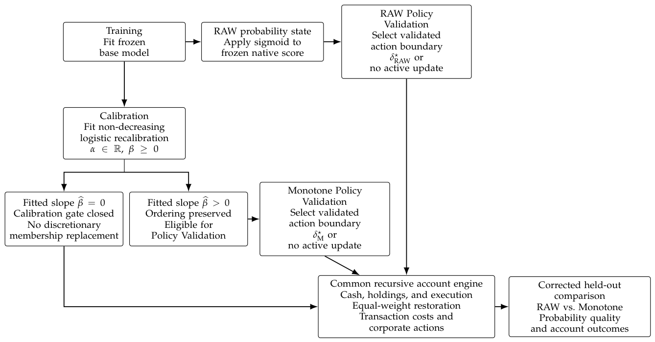
Figure 2.
Held-out Brier-score differences by model and period. Negative values favor monotone recalibration.
Figure 2.
Held-out Brier-score differences by model and period. Negative values favor monotone recalibration.
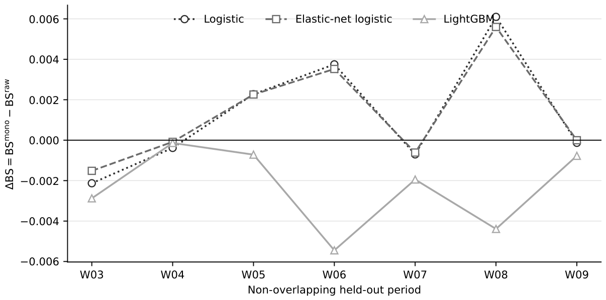
Figure 3.
Pooled held-out reliability diagrams by model. Bin counts are shown for populated bins with at least 50 observations. Curves closer to the diagonal indicate better calibration. Curves pool seven periods within each model and are diagnostic rather than inferential.
Figure 3.
Pooled held-out reliability diagrams by model. Bin counts are shown for populated bins with at least 50 observations. Curves closer to the diagonal indicate better calibration. Curves pool seven periods within each model and are diagnostic rather than inferential.
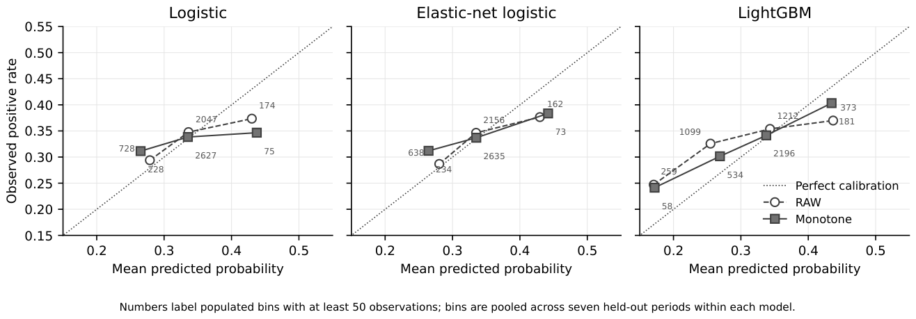
Figure 4.
Constrained recalibration slopes. A recorded zero denotes a KKT boundary solution and a closed gate; a positive value denotes an interior solution and an open gate.
Figure 4.
Constrained recalibration slopes. A recorded zero denotes a KKT boundary solution and a closed gate; a positive value denotes an interior solution and an open gate.
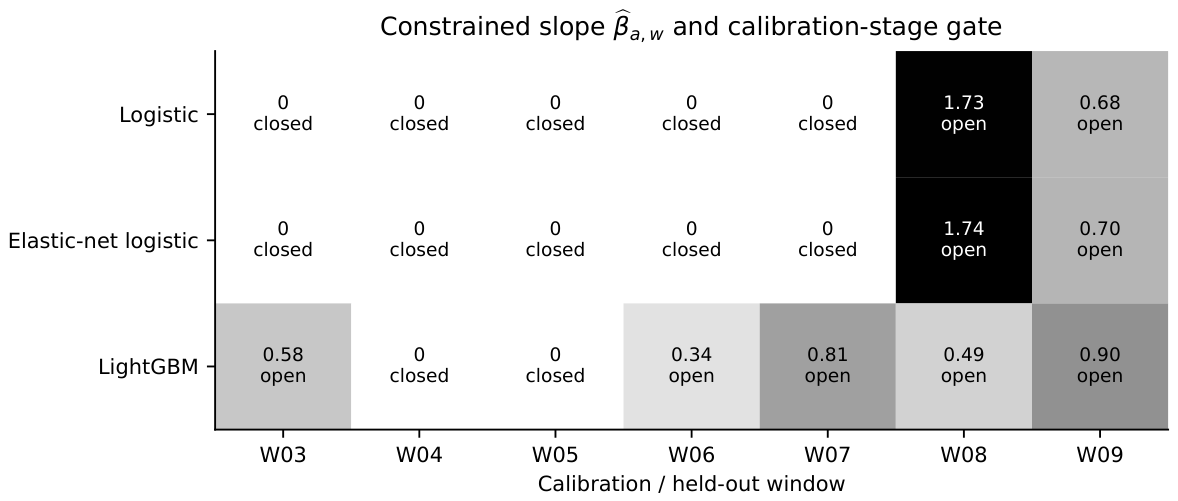
Figure 5.
Held-out hold-or-replace action-state comparison for the two prespecified primary policy models. Rows show RAW actions and columns show corrected monotone actions.
Figure 5.
Held-out hold-or-replace action-state comparison for the two prespecified primary policy models. Rows show RAW actions and columns show corrected monotone actions.
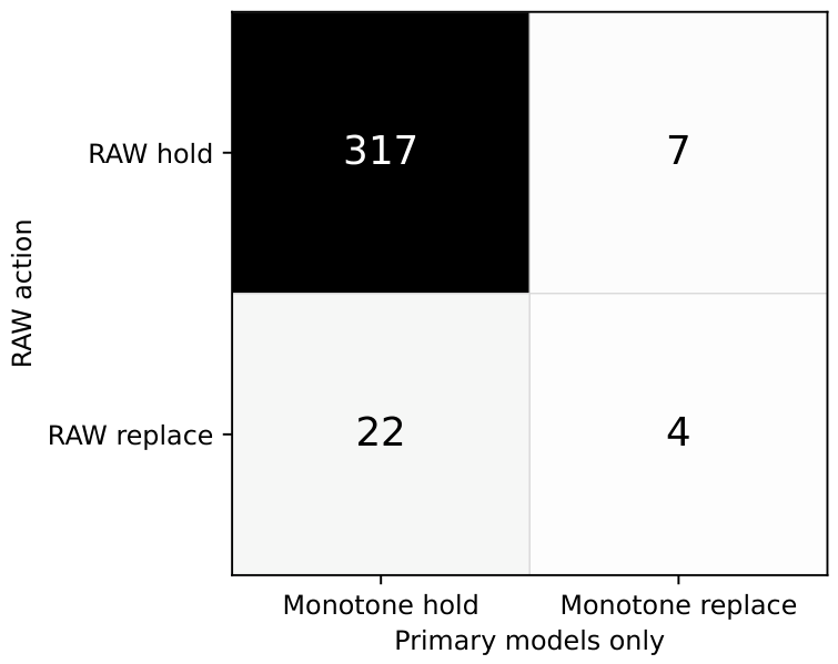
Figure 6.
Net differences by primary policy model and held-out period. Diamonds show the within-period average of elastic-net logistic and LightGBM; positive values favor the Monotone policy.
Figure 6.
Net differences by primary policy model and held-out period. Diamonds show the within-period average of elastic-net logistic and LightGBM; positive values favor the Monotone policy.
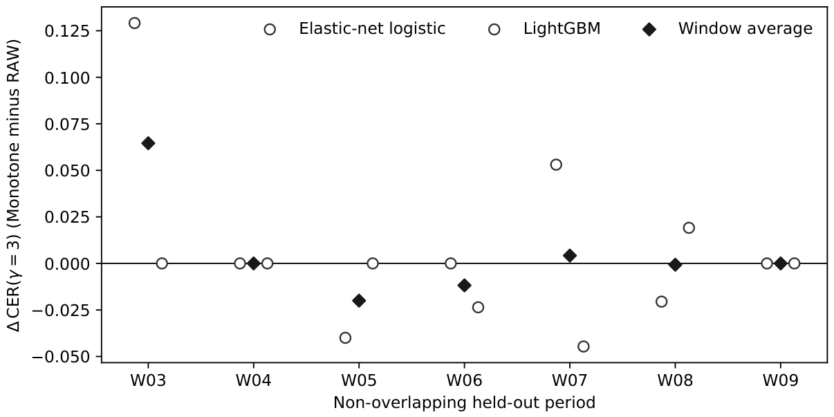

Table 1.
Component-level positioning relative to representative literature streams cited in this section. The comparison summarizes the roles emphasized by the cited studies and is not intended as an exhaustive claim about every paper in each stream.
Table 1.
Component-level positioning relative to representative literature streams cited in this section. The comparison summarizes the roles emphasized by the cited studies and is not intended as an exhaustive claim about every paper in each stream.
| Representative stream | Primary emphasis | Component carried into the present protocol | Integration point addressed here |
|---|---|---|---|
| Post-hoc / monotone calibration [9,14,15] | Probability reliability and, for monotone methods, ordering preservation | Non-decreasing score-to-probability map | Calibration is linked to an explicit action gate and later portfolio decision stages |
| Selective prediction [11,25] | Abstention when predictive evidence is insufficient | Explicit no-action behavior | Abstention is separated into Calibration-stage gate closure and Policy-Validation no-active-update selection |
| Financial threshold / no-trade / turnover control [7,12,13] | Restraining costly or weakly justified portfolio actions | Turnover eligibility and no-active-update option | Action evidence is defined by a calibrated candidate–holding probability margin and selected on an independent stage |
| Predict-then-optimize / decision-focused learning [17,18] | Alignment of predictive outputs with downstream decisions | Explicit downstream economic criterion | Training, recalibration, policy selection, and held-out account evaluation remain stage-separated and auditable rather than end-to-end |
| This study | Auditable deployment decision support | All components above | Matched RAW/Monotone recursive-account audit links probability quality, action coverage, turnover, costs, and economic outcomes |
Table 2.
Protocol provenance for principal fixed design choices. The listed constants were unchanged by the audit-triggered correction and are not selected from the corrected held-out outcomes. The audit-triggered monotone correction itself is not classified as a pre-held-out design choice; it was introduced after the original held-out outputs had been viewed, as disclosed in Section 5.2.
Table 2.
Protocol provenance for principal fixed design choices. The listed constants were unchanged by the audit-triggered correction and are not selected from the corrected held-out outcomes. The audit-triggered monotone correction itself is not classified as a pre-held-out design choice; it was introduced after the original held-out outputs had been viewed, as disclosed in Section 5.2.
| Design element | Frozen value | Protocol role | Fixed before held-out evaluation? |
|---|---|---|---|
| Temporal architecture | 1008 Training, 126 Calibration, 252 Policy Validation, 252 held-out trading days; 252-day rolling step | Separates model fitting, recalibration, policy selection, and evaluation in time | Yes |
| Prediction / rebalance horizon | 10 trading days | Uses a common horizon for labels, rebalance decisions, and account-return periodization | Yes |
| Portfolio action budget | , , long-only, equal-weight restoration | Isolates membership authorization and limits discretionary replacement to one pair per rebalance | Yes |
| Policy boundary set | Nine finite boundaries from 0 to 0.15 (Equation 10) plus NAU | Candidate set searched only in Policy Validation; NAU is the explicit no-active-update policy | Yes |
| Turnover eligibility | Annualized one-way active-member turnover | Feasibility filter applied before validation-CER maximization | Yes |
| Economic criterion | Primary ; sensitivity | Net CER selects the Policy Validation boundary; sensitivity values are reporting-only checks | Yes |
| Execution-cost model | 5 bp commission and 5 bp slippage per side; ETF stamp tax 0 | Shared account-cost semantics for RAW and Monotone paths | Yes |
| Deterministic tie rules | ETF code order for ranking ties; largest boundary for CER ties within tolerance | Prevents discretionary tie resolution after outcomes are observed | Yes |
| Model-selection grids | Frozen logistic, elastic-net, and LightGBM grids in Supplementary Table S4 | Hyperparameters selected by chronological Training-only cross-validation | Yes |
Table 3.
Stage-specific objectives and information flow.
| Stage | Quantity fitted or selected | Criterion / role | Held-out outcomes used within stage? |
|---|---|---|---|
| Training | Base model and hyperparameters | Three chronological folds; mean binary log loss | No |
| Calibration | and gate state | Calibration log loss with the exact non-negative boundary allowed | No |
| Policy Validation | or NAU | Maximize net among turnover-eligible policies | No |
| Held-out evaluation | No fitting or selection | Brier score primary for probability quality; ECE/REL and calibration diagnostics supplementary; activity, costs, and CER characterize deployment outcomes | Evaluation only |
Table 4.
Exact temporal boundaries. Cal. denotes Calibration and Policy denotes Policy Validation.
| Window | Train start | Train end | Cal. start | Cal. end | Policy start | Policy end | Held-out start | Held-out end |
|---|---|---|---|---|---|---|---|---|
| W03 | 2013-01-15 | 2017-03-10 | 2017-03-13 | 2017-09-11 | 2017-09-12 | 2018-09-20 | 2018-09-21 | 2019-10-11 |
| W04 | 2014-02-07 | 2018-03-21 | 2018-03-22 | 2018-09-20 | 2018-09-21 | 2019-10-11 | 2019-10-14 | 2020-10-26 |
| W05 | 2015-02-12 | 2019-04-03 | 2019-04-04 | 2019-10-11 | 2019-10-14 | 2020-10-26 | 2020-10-27 | 2021-11-08 |
| W06 | 2016-03-01 | 2020-04-16 | 2020-04-17 | 2020-10-26 | 2020-10-27 | 2021-11-08 | 2021-11-09 | 2022-11-21 |
| W07 | 2017-03-13 | 2021-04-29 | 2021-04-30 | 2021-11-08 | 2021-11-09 | 2022-11-21 | 2022-11-22 | 2023-12-04 |
| W08 | 2018-03-22 | 2022-05-18 | 2022-05-19 | 2022-11-21 | 2022-11-22 | 2023-12-04 | 2023-12-05 | 2024-12-18 |
| W09 | 2019-04-04 | 2023-05-30 | 2023-05-31 | 2023-12-04 | 2023-12-05 | 2024-12-18 | 2024-12-19 | 2025-12-31 |
Table 5.
Held-out probability changes and grouped Brier diagnostics. BS, ECE, and REL improvements correspond to negative Monotone-minus-RAW changes; RES improvement corresponds to a positive change.
Table 5.
Held-out probability changes and grouped Brier diagnostics. BS, ECE, and REL improvements correspond to negative Monotone-minus-RAW changes; RES improvement corresponds to a positive change.
| Slope state | n | BS improved | ECE improved | REL improved | RES improved | Mean | Mean |
|---|---|---|---|---|---|---|---|
| All groups | 21 | 15 | 17 | 19 | 3 | 0.000079 | -0.020380 |
| Positive slope () | 9 | 7 | 7 | 7 | 3 | -0.000429 | -0.019164 |
| Zero boundary () | 12 | 8 | 10 | 12 | 0 | 0.000461 | -0.021292 |
Table 6.
Constrained slope and gate states by base model. Calibration area under the receiver operating characteristic curve (AUC) is reported only as a diagnostic and is not a second gate.
Table 6.
Constrained slope and gate states by base model. Calibration area under the receiver operating characteristic curve (AUC) is reported only as a diagnostic and is not a second gate.
| Model | Groups | Median | Median Cal. AUC | ||
|---|---|---|---|---|---|
| Elastic-net logistic | 7 | 2 | 5 | 0.000 | 0.474 |
| LightGBM | 7 | 5 | 2 | 0.487 | 0.544 |
| Logistic | 7 | 2 | 5 | 0.000 | 0.461 |
Table 7.
Two-stage abstention and realized held-out policy pathways for the two prespecified primary policy models.
Table 7.
Two-stage abstention and realized held-out policy pathways for the two prespecified primary policy models.
| Pathway | Criterion | Groups | Held-out status |
|---|---|---|---|
| Calibration-gated abstention | 7 | No discretionary replacement | |
| Policy-validated abstention | ; selected NAU | 5 | No discretionary replacement |
| Policy-authorized, no held-out trigger | ; finite selected delta | 0 | No realized replacement |
| Policy-authorized updating | ; finite selected delta | 2 | At least one realized replacement |
Table 8.
Gate state, selected monotone policy, and realized action path for all 21 model–period groups. Reader-facing labels replace the machine-readable audit codes retained in the source data.
Table 8.
Gate state, selected monotone policy, and realized action path for all 21 model–period groups. Reader-facing labels replace the machine-readable audit codes retained in the source data.
| Window | Model | Gate | Selected policy | Active replacements |
|---|---|---|---|---|
| W03 | Elastic-net logistic | Closed () | No active update | 0 |
| W03 | LightGBM | Open | No active update | 0 |
| W03 | Logistic | Closed () | No active update | 0 |
| W04 | Elastic-net logistic | Closed () | No active update | 0 |
| W04 | LightGBM | Closed () | No active update | 0 |
| W04 | Logistic | Closed () | No active update | 0 |
| W05 | Elastic-net logistic | Closed () | No active update | 0 |
| W05 | LightGBM | Closed () | No active update | 0 |
| W05 | Logistic | Closed () | No active update | 0 |
| W06 | Elastic-net logistic | Closed () | No active update | 0 |
| W06 | LightGBM | Open | No active update | 0 |
| W06 | Logistic | Closed () | No active update | 0 |
| W07 | Elastic-net logistic | Closed () | No active update | 0 |
| W07 | LightGBM | Open | 10 | |
| W07 | Logistic | Closed () | No active update | 0 |
| W08 | Elastic-net logistic | Open | No active update | 0 |
| W08 | LightGBM | Open | 1 | |
| W08 | Logistic | Open | No active update | 0 |
| W09 | Elastic-net logistic | Open | No active update | 0 |
| W09 | LightGBM | Open | No active update | 0 |
| W09 | Logistic | Open | No active update | 0 |
Table 9.
Activity and path-level transaction costs for the 14 primary-model account paths. Monetary cost is also reported in basis points (bp; 1 bp = 0.01%) of the 1,000,000 initial equity per path.
Table 9.
Activity and path-level transaction costs for the 14 primary-model account paths. Monetary cost is also reported in basis points (bp; 1 bp = 0.01%) of the 1,000,000 initial equity per path.
| Method | Paths | Active replacements | Active turnover | Mean cost | Median cost | Mean/median bp |
|---|---|---|---|---|---|---|
| Monotone | 14 | 11 | 2.750 | 1935.12 | 1598.63 | 19.35/15.99 |
| RAW | 14 | 26 | 6.500 | 2520.27 | 1852.13 | 25.20/18.52 |
Table 10.
Window-averaged monotone-minus-RAW net differences. Positive values favor the Monotone policy.
Table 10.
Window-averaged monotone-minus-RAW net differences. Positive values favor the Monotone policy.
| Window | Direction | |
|---|---|---|
| W03 | 0.064567 | positive |
| W04 | 0.000000 | zero |
| W05 | -0.019990 | negative |
| W06 | -0.011791 | negative |
| W07 | 0.004219 | positive |
| W08 | -0.000699 | negative |
| W09 | 0.000000 | zero |
Disclaimer/Publisher’s Note: The statements, opinions and data contained in all publications are solely those of the individual author(s) and contributor(s) and not of MDPI and/or the editor(s). MDPI and/or the editor(s) disclaim responsibility for any injury to people or property resulting from any ideas, methods, instructions or products referred to in the content. |
© 2026 by the authors. Licensee MDPI, Basel, Switzerland. This article is an open access article distributed under the terms and conditions of the Creative Commons Attribution (CC BY) license (http://creativecommons.org/licenses/by/4.0/).
Copyright: This open access article is published under a Creative Commons CC BY 4.0 license, which permit the free download, distribution, and reuse, provided that the author and preprint are cited in any reuse.