

Submitted:
15 September 2026
Posted:
16 September 2026
You are already at the latest version
Abstract
The incompressible Navier–Stokes equations have recently been shown to admit finite-time singularities from smooth data under smooth bounded forcing. Since unbounded velocity gradients are physically inadmissible, the only element of the equations open to revision is the constitutive relation \(\sigma=-pI+F(\nabla u)\). From the Cauchy momentum equation we derive the most general \(F\) compatible with frame indifference, isotropy and the Cayley–Hamilton theorem, \(F=\alpha_1D+\alpha_2D\cdot D\) with invariant-dependent coefficients, and prove that the constant-coefficient second-order model \(\sigma=-pI+2\mu D+4\lambda D\cdot D\) violates the second law in three dimensions, is an exact gradient in two, and cannot bound velocity gradients. The improvement must therefore enter the linear coefficient, and the lowest-order admissible law is \(\sigma=-pI+2\mu(1+\tau^2 D: D) D+4\lambda\ D\cdot\ D\) with a material time \(\tau\). We prove that the second law requires \(\tau\ge|\lambda|/(\sqrt6\mu)\) and, by an exact block decomposition of the tangent operator, that monotonicity requires the sharp bound \(\tau\ge\sqrt{2/3}\,|\lambda|/\mu\), twice the thermodynamic one. Under it the momentum operator is strongly monotone with quartic growth, the equations lie in the Ladyzhenskaya–Lions class \(p=4\), solutions are global, unique and bounded, and the forced blow-up cannot occur. Exact solutions in simple shear and gravity-driven pipe flow give a two-measurement protocol for \(\tau\) and \(\lambda\) with an internal consistency test, and a strained vortex exhibits the arrest of collapse at strain rate \(1/\tau\). A boundary-layer theory consistent to second order shows that \(\lambda\) drops out exactly, that the flat-plate layer has a leading-edge regime \(\delta\propto x^{1/4}\), \(\tau_w\propto x^{-3/4}\) crossing over to Blasius scaling at \(\ell_\tau=\tau^2U^3/(2\nu)\), and that only the wedge flow \(U\propto x^{1/3}\) remains self-similar. Numerical solutions and experimental protocols are given.
Keywords:
Navier–Stokes equations
; constitutive relations
; non-Newtonian flows
; boundary layers
; regularity
; removal of finite-time blow-up
1. Introduction
1.1. The Navier–Stokes Equations and Their Limits
The equations that bear the names of Navier [15] and Stokes [24] have described the motion of incompressible viscous fluids for two centuries. Written in the tensor notation adopted throughout this paper, they read
where is the velocity, p the pressure, the density, the viscosity, the body force per unit mass, the gradient operator and the velocity gradient, so that is the convective acceleration. Their success is not in doubt. Direct numerical simulations of (1) reproduce turbulent statistics to within experimental accuracy at every Reynolds number that has so far been computed [14,18], and the equations underpin the whole of engineering fluid mechanics.
Whether (1) is complete, however, has been an open question since Leray [10] constructed weak solutions whose regularity he could not establish. The question was formalised by the Clay Mathematics Institute [7] and remained open until 8 September 2026, when a proof was announced, together with a formalisation in the Lean proof assistant, that a smooth incompressible fluid initially at rest, acted upon by a smooth bounded body force and possessing finite kinetic energy throughout, develops a singularity in finite time: the velocity becomes unbounded while the energy remains finite [17]. Closely related results for the Euler, Boussinesq and porous-medium equations were obtained independently at the same time [3]. The proof establishes statements C and D of the Clay formulation, i.e., blow-up under smooth forcing; the unforced problem remains open. The construction is a collapsing vortex whose core shrinks and accelerates without bound, its strain rate diverging as the singular time is approached.
For the physicist the mathematical statement has an immediate corollary. Infinite velocity and infinite velocity gradient are not attainable by any real liquid or gas: the incompressible equations are valid only for speeds well below the sound speed, and the Newtonian constitutive law from which the viscous term of (1) descends was derived, by Navier and by Stokes alike, under the assumption of a small velocity gradient. A model that can be driven by a bounded, smooth force into a state its own derivation excludes has, at that point, ceased to describe the fluid. The conclusion is not that the Navier–Stokes equations are wrong—they are demonstrably an excellent approximation over an enormous range of conditions—but that they are incomplete, in precisely the sense that they lack the physics that intervenes when the velocity gradient becomes large. The purpose of this paper is to identify that physics from first principles, to formulate the improved governing equations that result, to prove that they have the regularity the Navier–Stokes equations lack, and to work out their consequences in a form that can be tested.
1.2. Where the Equations Can Be Changed
The derivation of (1) contains one, and only one, hypothesis that is not a conservation law. Mass conservation for an incompressible fluid is ; momentum conservation for any continuum is Cauchy’s equation
with the Cauchy stress. Neither admits adjustment. The physical content of a particular fluid enters solely through the constitutive relation
and the choice , linear in the velocity gradient, is what turns (2) into (1). This observation was made forcefully by Sun [26], who proposed retaining the next term permitted by the Cayley–Hamilton theorem and obtained with the rate-of-strain tensor and a new “second-order viscosity”. The model is a particular member of the class of isotropic tensor functions studied by Reiner [20] and Rivlin [21], in which is the cross-viscosity, and it raises exactly the right question: given that only can be changed, what form must take?
1.3. Programme and Results
We answer this question in three steps, summarised in Figure 1.
First (§Section 3) we derive the most general compatible with material frame indifference, isotropy and the second law. Frame indifference removes the dependence on the spin, so that ; the representation theorem of Rivlin Ericksen [22] and the Cayley–Hamilton theorem reduce to with coefficients that are functions of the two nontrivial invariants of ; and the second law imposes a dissipation inequality on those coefficients.
Second (§Section 4) we show that the constant-coefficient second-order model cannot be the improvement sought. Three theorems establish that with constant the model violates the second law in three dimensions, that in two dimensions the term is an exact gradient so that the model is dynamically identical to Navier–Stokes, and that a quadratic stress produces a cubic, non-coercive dissipation that cannot bound the velocity gradient. The second of these has a consequence that must be stated plainly: every two-dimensional result obtained from the constant-coefficient model, including the wedge-flow boundary layers of Sun [26], is an artefact of an inconsistent reduction in which the modified pressure was not carried through the transverse momentum balance. The improvement must therefore enter the coefficient of the linear term.
Third (§§Section 5Section 6) we formulate the lowest-order admissible law,
in which is a material time—the reciprocal of the strain rate beyond which the fluid stiffens against further deformation—and derive its governing equations. We prove that the second law requires (theorem 3) and, by an exact decomposition of the tangent stress operator into decoupled blocks, that monotonicity of the stress—the condition for Hadamard well-posedness—requires (theorem 4), exactly twice the thermodynamic bound. Under the latter condition the momentum operator is strongly monotone with quartic growth and the equations belong to the class introduced by Ladyzhenskaya [9] and Lions [11], for which global existence and uniqueness are known for growth exponent ; here . The forced finite-time blow-up of the Navier–Stokes equations therefore cannot occur (theorem 5). The mechanism is transparent: the effective viscosity grows with the strain rate, so that the viscous stress in a collapsing core eventually grows as and overwhelms the inertial amplification, which grows as . The collapse is arrested at strain rate and core size ; the Navier–Stokes equations, which contain no such scale, can be driven past it.
The remainder of the paper develops the theory to the point of experimental test. Section 7 gives exact solutions in simple shear and in gravity-driven pipe flow, from which a two-measurement protocol determines and separately and the inequality provides an internal consistency check; it also presents the stiffened Burgers vortex as a numerical example of arrested collapse. Section 8 develops the boundary-layer theory of the new equations consistently to second order in the layer thickness. Its principal results are that drops out of the boundary-layer equations identically, that the flat-plate layer has a leading-edge regime with and that crosses over to Blasius scaling at the material length , and that among the Falkner–Skan wedge flows only remains exactly self-similar. The non-similar flat-plate equations are solved by marching, the self-similar wedge is tabulated, and both are shown to agree with their analytic limits. Section 9 discusses the relation of the theory to turbulence and to direct numerical simulation, its regime of validity, its extensions, and what has and has not been proved.
2. Kinematics, Balance Laws and Notation
2.1. Tensor Notation
We follow the conventions of Sun [26]. Vectors and second-order tensors are set in boldface; () are the Cartesian base vectors and summation over repeated indices is implied. The gradient operator is and acts as a vector: the velocity gradient is the outer (dyadic) product
The symmetric and antisymmetric parts of the velocity gradient are the rate-of-strain tensor and the spin tensor,
For second-order tensors , the single and double contractions are and ; the divergence of a tensor is the contraction with ∇ on the right, , which for a symmetric tensor coincides with the left divergence . The convective acceleration is ; the frequently written is avoided because it obscures the fact that the operand is the tensor . The Frobenius norm is , the Laplacian is , and powers are , .
The principal invariants of are
For an incompressible fluid , so that and, by the Cayley–Hamilton identity traced, . Throughout we use and as the two independent invariants.
2.2. Balance Laws
For a continuum of constant density the balances of mass and linear momentum are
and the balance of angular momentum, in the absence of body couples, is . These hold for every continuum and admit no adjustment. Under isothermal conditions the second law, in the form of the Clausius–Duhem inequality with Helmholtz free energy [27], reduces to
and for a fluid without elastic energy storage ( in isothermal motion) to the dissipation inequality .
2.3. Constitutive Relation
To close (8)–() a constitutive relation must be supplied. For a fluid without memory the stress is a function of the present velocity gradient,
in which p is the constraint pressure enforcing (8) and is the extra stress. The Newtonian choice gives (1), because for solenoidal . Every other property of a particular fluid enters through , and it is to the determination of that we now turn.
3. The Admissible Form of the Constitutive Relation
Three principles constrain : material frame indifference, material symmetry (isotropy), and the second law. We take them in turn. None of the results of this section is new in continuum mechanics [16,22,27], but assembling them in the present context is what determines the structure of the improved equations, and the lemma on that closes the section is used repeatedly.
3.1. Material Frame Indifference
Under a superposed rigid motion , with orthogonal, the velocity gradient transforms as
where is antisymmetric. The symmetric part transforms objectively, , while the spin acquires the frame rotation, . Since is arbitrary, the requirement can hold for all observers only if does not depend on [16]:
This is the first structural fact: whatever nonlinearity is added to the Newtonian law must be built from alone. Models in which the stress depends on through combinations other than are not constitutive relations for a fluid but artefacts of a particular observer.
3.2. Isotropy and the Cayley–Hamilton Theorem
For an isotropic fluid the second condition in (13) holds for all orthogonal , so that is an isotropic tensor function of the single symmetric tensor . The representation theorem of Rivlin Ericksen [22] states that every such function is a polynomial in with coefficients that are functions of the invariants, and the Cayley–Hamilton theorem [5],
reduces every power , , to a combination of , and . Hence
with for an incompressible fluid. The term is an isotropic stress and is absorbed into the constraint pressure p. Two remarks are essential for what follows.
First, (15) is exhaustive: there is no further term to add. The Navier–Stokes equations correspond to , ; the model of Sun [26] to , with both constant; the fluid of Reiner [20] and Rivlin [21], of which the latter is a special case, to arbitrary .
Second, the coefficients are functions of the invariants, not constants. The historical reason for treating them as constants is that in the small-gradient limit and the invariant dependence is a higher-order correction. Precisely because the problem before us is the large-gradient limit, the invariant dependence of is not a refinement but the heart of the matter.
3.3. The Second Law
Whatever are chosen, they must satisfy (17) identically. The following lemma converts (17) into an explicit condition.
Lemma 1
(bound on the cubic invariant). For every traceless symmetric in three dimensions,
with equality if and only if has eigenvalues proportional to , i.e., is an axisymmetric extension or compression.
Proof.
In the eigenbasis of , with eigenvalues and , one has , by the identity . It suffices to maximise on the circle , . The Lagrange conditions for cyclic imply, on subtracting pairs, , so that at an extremum at least two eigenvalues coincide. With and one finds and . Homogeneity of degree three in gives the general statement. □
Corollary 1.
For traceless symmetric the largest eigenvalue satisfies , with equality in the same configuration.
Proof.
Maximise subject to , : by Cauchy–Schwarz , so . □
3.4. Consequence: the Linear Coefficient Must Depend on the Strain Rate
Inequality (17) with lemma 1 gives the necessary and sufficient condition
because the cubic invariant can be made to take either sign at the extremal orientation. Equation (19) is the key structural constraint of the theory. If is a nonzero constant, then must grow at least linearly with ; a constant is excluded. In other words, one cannot add a second-order term to the Newtonian law without at the same time modifying the coefficient of the first-order term, and the modification must make the fluid stiffer at large strain rate. The next section makes the failure of the constant-coefficient model explicit; §Section 5 then chooses the simplest that satisfies (19).
4. The Constant-Coefficient Second-Order Model
The model with constant [26] is the natural first candidate for an improved law, and it is instructive to see precisely why it fails. The three theorems of this section are independent of one another; each alone would disqualify the model as the sought-for completion of the Navier–Stokes equations.
4.1. Violation of the Second Law
Theorem 1
(thermodynamic inadmissibility). For constant and constant , the dissipation is negative for some traceless symmetric . Specifically, with ,
Proof.
Immediate from lemma 1: at the extremal configuration , the sign being chosen opposite to that of . □
The failure is not marginal. For any fluid with there exists an axisymmetric straining motion of finite strain rate beyond which the model generates mechanical energy from nothing. This is the well-known thermodynamic defect of the Reiner–Rivlin fluid with constant cross-viscosity [6,27]. It is worth noting why it escaped detection in Sun [26]: the entropy inequality was verified there only for two-dimensional flow, Equation (25) of that paper, where vanishes identically by continuity (). The check is vacuous in two dimensions and fails in three.
4.2. Dynamical Invisibility in Two Dimensions
Theorem 2
(planar flows). For every planar incompressible flow with ,
Consequently the equations of motion of the constant-coefficient model coincide, in planar flow, with the Navier–Stokes equations under the substitution .
Proof.
The in-plane part of is a traceless symmetric tensor, for which the Cayley–Hamilton theorem reads ; since when , one has . In components, with and , and . The components involving vanish. Taking the divergence, with , gives (21) with . Substituting in () then gives . □
The identity was also confirmed by symbolic computation for an arbitrary stream function (appendix ). Its consequence for the two-dimensional results of Sun [26] is unavoidable. The wedge-flow boundary-layer equation of that paper, its Equation (27), retains a term in the streamwise momentum balance while taking the pressure to be the outer pressure . But at the same order in the layer thickness the transverse momentum balance reads
where , and substituting this into the streamwise balance gives , which cancels the retained term identically. The consistent boundary-layer equations are Prandtl’s, unchanged; the wall shear parameter is for every value of the parameter of that paper, and the “turbulent” profiles of its Figure 2 and Table 1 are not predictions of the model. We return to the boundary-layer reduction in §Section 8, where it is carried out consistently for the improved law.
The physical content of theorem 2 is that in planar flow the second-order stress is isotropic in the plane: the first normal-stress difference of a Reiner–Rivlin fluid vanishes identically [2]. The term is dynamically active only through genuinely three-dimensional straining, in which the three eigenvalues of are distinct.
4.3. Failure to Bound the Velocity Gradient
The third defect is not thermodynamic but analytic. Even where , the dissipation of the constant-coefficient model is at most cubic in and its sign is indefinite in the cubic term; it therefore provides no better a priori control of than the quadratic dissipation of the Navier–Stokes equations, which is exactly the control that fails to prevent blow-up. A term quadratic in in the stress can never be coercive, because is not monotone: the tangent map has , which takes both signs.
Taken together, theorems 1 and 2 and the observation just made show that the Cayley–Hamilton term cannot by itself supply the missing physics. Condition (19) locates where the physics must go: in the coefficient of .
5. The Improved Constitutive Relation and the Governing Equations
5.1. Choice of the Coefficients
Condition (19) requires to grow at least linearly in if , and the regularity theory of §Section 6 will require, independently of , that grow at least as . The coefficient is a scalar isotropic function of and may depend on both invariants. Dependence on , which is odd under , would make the linear coefficient different for extension and compression; we exclude it on the grounds that a fluid with no preferred direction should resist a straining motion and its reverse equally, and retain only dependence on . The lowest-order analytic correction is then
which gives the constitutive relation
Three material constants appear: the Newtonian viscosity (dimension M/LT), the cross-viscosity (dimension M/L, the “second-order viscosity coefficient” of Sun [26]), and a material time (dimension T). The combination is the strain rate at which the effective viscosity has doubled; below it the fluid is Newtonian to , above it the fluid stiffens. Higher even powers, , are admissible and would refine (24) at still larger strain rate; nothing below depends on their absence except the numerical values of the constants in the regularity estimates, and the theory of §Section 6 applies to any with growth exponent .
5.2. Thermodynamic Admissibility
Theorem 3
(second law). The dissipation of (24),
is non-negative for every traceless symmetric if and only if
Proof.
Let . By lemma 1, , and by the inequality of arithmetic and geometric means , so that under (26). Conversely, at the extremal of lemma 1 with the sign of opposite to that of , , a quadratic in s whose discriminant is ; it is negative for some s precisely when . At the bracket is the perfect square , vanishing at . □
The theorem couples the two new constants. A fluid with cross-viscosity cannot exist without a gradient-stiffening time of at least ; the model of Sun [26] is the limit , excluded unless . Figure 2(a) shows the admissible region in the plane; Figure 2(b) shows along the worst orientation for several . A second, stronger boundary also appears in the figure; it is the monotonicity condition of theorem 4, to which we come in §Section 6.
5.3. Governing Equations
Substituting (24) into () and using for the Newtonian part, with and (dimension L2), we obtain the improved governing equations
In Cartesian components,
where . The last term is identical to that of Sun [26], Equation (16) there, since ; the penultimate term is new. Expanding the derivatives,
which exhibits the structure of the stiffening term: an isotropic viscosity enhancement plus a force directed along the gradient of . Explicit Cartesian and cylindrical component forms are given in appendix .
5.4. Dimensionless Form
is the parameter introduced by Sun [26]; it depends on the length scale alone, as noted there. is a gradient number, the ratio of the flow strain rate to the material strain rate ; it plays the role that the Weissenberg number plays for viscoelastic liquids, although the physics is different, since (24) has no memory. The admissibility conditions read (second law) and (monotonicity). Relative to the Newtonian viscous term the stiffening term is , with the dimensionless local strain rate: it is negligible where the local strain rate is small compared with and dominant where it is large, irrespective of the Reynolds number. This is the decisive difference from the term , which is fixed by the length scale.
5.5. Energy Identity
Taking the inner product of the momentum equation with , integrating over a domain with no-slip walls or periodic boundaries, and using and the symmetry of ,
By theorem 3, whenever the integrand is bounded below by with (take and use the arithmetic–geometric bound with the remaining fractions). Hence for any bounded forcing on ,
This is the estimate that the Navier–Stokes equations lack, and it is the source of everything in §Section 6.
5.6. Limiting Cases
6. Monotonicity, Well-Posedness and the Removal of Blow-Up
Thermodynamic admissibility guarantees that the fluid dissipates energy, but not that the equations are well posed. The additional requirement is that the extra stress
be a monotone function of : for all traceless symmetric ,
Monotonicity is what makes the viscous operator elliptic in the sense required for the initial-value problem to be well posed in the sense of Hadamard: where it fails, the linearised equations admit modes that grow without bound at arbitrarily small scales, and the constitutive relation is unstable [8]. For the differentiable at hand, (35) holds if and only if the tangent (Gâteaux) operator is positive semidefinite,
since .
6.1. The Tangent Operator
Differentiating,
so that, using ,
The first two terms are non-negative; the third is of indefinite sign and is the only route by which monotonicity can fail.
6.2. The Sharp Monotonicity Theorem
Theorem 4
(monotonicity). The extra stress of (24) is monotone on traceless symmetric tensors if and only if
For it is strongly monotone: for all ,
Proof.
Fix and work in its eigenbasis, , , . Write , with , , and off-diagonal with entries , . The three terms of (38) decouple exactly between the diagonal and off-diagonal parts: ; involves only ; and contains no cross term. Hence with
where in (41) k is the index complementary to and .
Off-diagonal block. for all if and only if for each k, i.e., over both signs of (replace by ). By corollary 1, with equality attainable, so the condition for all of norm s is
Diagonal block. Parametrise the traceless diagonal tensors by an angle: , and let and be the orthonormal basis of the two-dimensional space of traceless diagonal tensors. Using , , and the triple-angle formulae,
With , () becomes the quadratic form
where , and . Its trace is positive and its determinant is
Since , the determinant is non-negative for all whenever , and it is negative at when . Thus the diagonal block is positive semidefinite for all of norm s under exactly the same condition (43) as the off-diagonal block.
The theorem is sharp: at the form vanishes when is the axisymmetric tensor of norm and is any shear in a plane containing the axis. In physical terms, for an axisymmetric strain and a perturbing shear in a plane containing the axis, contributes to the shear stress, an effective viscosity reduction; the condition for all is precisely . This configuration—a stretched vortex—is exactly the geometry of the blow-up construction, and we return to it in §Section 7.4. An independent numerical minimisation of over all (appendix ) located the threshold at , in agreement with , and reproduced the bound (40) to four significant figures at and .
Corollary 2
(coercivity and growth). For there are constants depending only on such that for all traceless symmetric ,
Proof. (47) is theorem 3 with a fraction of the quartic term retained after the arithmetic–geometric step; () follows from ; () follows by integrating (40) along the segment from to after retaining, in the proof of theorem 4, the fraction of not consumed by the arithmetic–geometric bound (for a positive fraction is available). □
6.3. Global Existence, Uniqueness and Regularity
Theorem 5
(global well-posedness). Let , let , and let be a smooth divergence-free initial velocity and a smooth bounded body force. Then for every the system (27) possesses a unique weak solution on with
satisfying the energy identity (32). Moreover the solution is strong,
so that the enstrophy is bounded uniformly on for every T.
Proof.
The proof follows the monotone-operator method of Ladyzhenskaya [9] and Lions [11], chapter 2, §5, and we indicate only where the hypotheses enter. Existence. Galerkin approximations satisfy the energy identity, and by (47) they are bounded in (Korn’s inequality on the torus gives ). By (), is bounded in , and the convective term is bounded in because by the Sobolev embedding . Hence is bounded in , the Aubin–Lions lemma gives strong convergence in , the convective term passes to the limit, and monotonicity (35) with Minty’s trick identifies the weak limit of as . Uniqueness. For two solutions let . Subtracting the equations, testing with and using (),
The right side is bounded by by interpolation between and and Young’s inequality; since , Gronwall’s lemma gives . (For general growth exponent p the same argument closes for ; here .) Regularity. On the torus one may test the equation with ; the viscous term yields, by () applied pointwise to difference quotients, the positive quantity , and the convective term is bounded by , which is absorbed for exactly as in Málek et al. [12]; see also Málek et al. [13], chapter 5. The estimate closes with and . □
Corollary 3
(no finite-time blow-up). Under the hypotheses of theorem 5, the velocity gradient of the improved equations satisfies and for every . The finite-time singularity of the Navier–Stokes equations under smooth bounded forcing [17], in which the velocity becomes unbounded, cannot occur: for the Navier–Stokes equations bounded enstrophy implies regularity by the Ladyzhenskaya–Prodi–Serrin criterion, so any Navier–Stokes blow-up is accompanied by unbounded enstrophy, whereas the enstrophy of the improved equations is bounded on every finite interval.
6.4. Physical Mechanism and the Regularisation Scale
The mathematics has a simple physical reading, sketched in Figure 3. In the blow-up solution a vortex core of size ℓ collapses under an axial strain, and its azimuthal velocity v grows so that stays finite. The strain rate in the core is , the inertial (stretching) amplification of vorticity is proportional to , and the Newtonian viscous stress that opposes it is proportional to : viscosity loses at small scale, and nothing in (1) stops the collapse. In (27) the viscous stress is , which grows as and overtakes the amplification once . The collapse is arrested at strain rate and the core reaches a minimum size
the length at which the Newtonian viscous time equals the material time . This is the regularisation scale of the theory. It is a property of the fluid, not of the flow, and it plays for the improved equations the role that the Kolmogorov scale plays for a turbulent flow: whereas can be made arbitrarily small by increasing the dissipation rate , cannot. In a turbulent flow with the stiffening term is negligible everywhere and (27) is indistinguishable from (1); it acts only where the cascade, or a forced collapse, would otherwise drive the strain rate past .
7. Exact Solutions and the Determination of the Material Constants
The theory contains two constants beyond the Newtonian viscosity. Both must be measured, and the measurements must be consistent with theorem 4. This section gives the exact solutions on which the measurements can be based, and a numerical example—the stiffened Burgers vortex—that exhibits the arrest of collapse in a genuinely three-dimensional flow.
7.1. Simple Shear and Viscometry
For the steady simple shear the velocity gradient is , so
Figure 4 displays them. Three remarks follow. (i) The shear viscosity increases quadratically with the shear rate; the material time is read directly from the rate at which it has doubled, or from the curvature of at small rate. (ii) The first normal-stress difference vanishes identically—this is theorem 2 again—and the second is quadratic in the rate with coefficient . The measurement of therefore gives including its sign. (iii) The consistency condition becomes, in terms of measurable quantities,
which is a falsifiable statement about a single rheogram. A fluid that showed a measurable without shear thickening at the rate would violate the theory.
7.2. Gravity-Driven Flow in an Inclined Pipe
Consider the steady flow of the fluid down an infinitely long circular pipe of radius R inclined at an angle to the horizontal, with no imposed pressure gradient—the configuration proposed by Sun [26] for the determination of . We use cylindrical coordinates with along the pipe axis in the direction of the flow, so that the gravitational body force is , and seek by the semi-inverse method a solution . Then
and the nonzero stress components are
Continuity is satisfied identically. The three components of () are
Since the pipe is infinite and the ends are at equal pressure, ; the and r equations then give
where is the pressure on the axis; the hydrostatic term vanishes in a vertical pipe (), and we write for the wall pressure in that case. The z equation integrates once, with regularity at the axis, to
Equation (64) is a cubic for whose left side is strictly increasing in ; it has exactly one real root for every r, and the profile is obtained by quadrature from . Note the division of labour between the two constants: controls the velocity profile through (64) and does not enter it, because ; controls the transverse pressure distribution through (60) and enters that only through .
With the wall shear rate of Poiseuille flow , the dimensionless variables , and the parameter
(64) reads , and the flow rate and wall–axis pressure difference in the vertical pipe () are
with the Poiseuille flow rate. For , , and , which recovers Equation (47) of Sun [26], . For , and : the profile approaches that of a power-law fluid of index and the wall shear rate falls as . Table 2 and Figure 5 give the intermediate values.
7.3. Protocol for the Determination of and
The two exact solutions lead to the following procedure (Figure 6).
- 1.
- Measure in the Newtonian range, by any standard method.
- 2.
- In a vertical pipe of radius R, measure the flow rate Q under gravity alone, over a range of R (or of ) so that spans the range where departs from unity. Invert the first of (66), or read Table 2, to obtain and hence . Every pipe must return the same ; the collapse of against is the first test of the theory.
- 3.
- In the same pipe, measure the pressure difference between the wall and the axis in a cross-section, . With known, the second of (66) gives , including its sign.
- 4.
- Verify (theorem 4). Failure would indicate that the fluid is outside the class described by (24), for instance because it has memory.
- 5.
- Independently, in a rotational rheometer, measure and and compare with (56). The agreement of the two determinations of and of is the second test.
For low-viscosity liquids such as water no departure from Newtonian behaviour has been resolved by rheometry up to shear rates of order –, which places below roughly s and below about a micrometre; the theory is therefore not in conflict with any existing measurement on simple liquids, and its regularisation scale, while small, remains three orders of magnitude above the molecular scale at which the continuum description itself would fail. For suspensions and other complex fluids that shear-thicken at accessible rates, all of the quantities in steps 2–5 are measurable with existing apparatus.
7.4. A Strained Vortex: Arrest of Collapse
The Burgers vortex [4] is the exact steady Navier–Stokes solution in which an axisymmetric vortex is held against viscous diffusion by the irrotational strain . It is the simplest model of the stretched vortex tubes that populate turbulent flows and, in the geometry of OpenAI [17], of the collapsing core of the blow-up solution, in which grows without bound. We use it here as a three-dimensional test of the improved law with all terms active.
With the rate of strain is
so that and, because the strain part has , . The azimuthal shear stress is therefore
which makes explicit the observation following theorem 4: in a stretched vortex the cross-viscosity reduces the effective viscosity by , and it is the term that keeps the effective viscosity positive for all precisely when . The azimuthal momentum equation, with the radial and axial equations satisfied by a pressure that is a function of r and z alone, is
with and as . In terms of the Burgers radius , the scaled variables , , and the parameters , and , this becomes
whose Newtonian solution is with peak vorticity . Equation (70) was solved by a finite-difference Newton iteration in the regular variable (appendix ); Figure 7 shows the result for .
The peak vorticity of the Burgers vortex is : for a given circulation it grows linearly with the strain rate, without limit, which is the elementary form of the collapse mechanism. In the improved law it is reduced by 2% at , 7% at , 18% at and 28% at , and the core radius (the position of the velocity maximum) grows from to over the same range. The reduction sets in when in the core reaches order one; since in the core is dominated by the azimuthal shear, of order , the onset is at , i.e., for the case shown, which is what the figure displays. The cross-viscosity, with the sign that reduces the effective viscosity, slightly intensifies the vortex at small but is overpowered by the stiffening as grows. Thus a vortex subjected to ever-increasing strain does not collapse: its core saturates at the size of (53) and its peak vorticity at the value set by the material time, rather than growing without bound with .
8. Boundary-Layer Theory
The boundary layer is where velocity gradients are largest in a high-Reynolds-number flow, and it is where Prandtl [19] showed that a viscous term, however small its coefficient, cannot be neglected. It is therefore the natural setting in which the improved law acts, and it is also the setting most amenable to experimental verification, since wall shear stress and boundary-layer profiles are routinely measured. This section derives the boundary-layer equations of (27) consistently, solves them for the flat plate and for wedge flows, and identifies the measurements that would confirm or refute the theory.
8.1. Order-of-Magnitude Analysis
Consider steady two-dimensional flow past a wall with outer velocity , and let be the layer thickness, L the streamwise length, . Prandtl’s estimates, listed in table I of Sun [26], are ; ; ; , in units of U and L. In planar flow
and the components of the two new stress operators are, to leading order,
The y-momentum equation determines the pressure variation across the layer. The term () produces , whose streamwise gradient is of the same order as () and, as shown in §Section 4, cancels it identically—this is theorem 2 in boundary-layer form. The term () produces a pressure variation whose streamwise gradient, , is smaller than (72) by a factor . We conclude:
Proposition 1
(boundary-layer equations). To leading order in ϵ, the boundary-layer equations of the improved system (27) are
with at and as . The cross-viscosity λ does not appear; the pressure across the layer is . The wall shear stress is
Equation (76) is Prandtl’s equation with the shear viscosity replaced by the viscometric function of (56). This is as it should be: within a thin layer the flow is locally a simple shear, and the only material function a simple shear can probe is . The corresponding equation for a power-law fluid was studied by Acrivos et al. [1]; the present case differs in possessing a Newtonian core at small rate, which produces the two-regime structure described next. The retained term is the largest in the equation wherever , and the parameter that measures its importance is
the correction is governed by , not by alone, and increases with Reynolds number at fixed gradient number because the layer thins.
8.2. The Flat Plate: Non-Similar Equations and the Material Length
For introduce the Blasius variables , , so that and . Then , and the natural streamwise scale is the material length
Substituting into (76), the standard non-similar form of the convective terms [23] gives
with at and as . For the stiffening term vanishes and (80) reduces to the Blasius equation; the flat plate “forgets” the material time downstream, because the wall shear rate falls below at . Upstream of the stiffening term dominates and a different similarity structure emerges.
8.2.1. Leading-Edge Similarity Solution
Seek with . Then , , , and one finds and , so that the right side of (80) is exactly. The term is while the Newtonian term vanishes as . The leading-edge problem is therefore
which is the boundary-layer equation of a power-law fluid of index in the form of Acrivos et al. [1]. Its numerical solution (appendix ) gives
The corresponding physical scalings are
where . The wall shear stress therefore varies as near the leading edge, more steeply than the Blasius , and the layer grows as , more slowly than : near the leading edge the shear-stiffened fluid behaves, in the boundary layer, like a fluid of higher viscosity that thins the layer and raises the friction. Figure 8 sketches the two regimes.
8.2.2. Numerical Solution and Crossover
Equation (80) was integrated by marching in X from , where the leading-edge solution (81) supplies the initial profile, to , with the streamwise derivatives discretised backward and the two-point boundary-value problem in at each station solved by collocation (appendix ). Table 1 and Figure 9 summarise the results. The skin-friction function follows the leading-edge law (83) to within for and approaches the Blasius value from below for , reaching at . Between the two it passes through a shallow minimum, at , some below Blasius: in the crossover region the wall shear rate has fallen below , so that the stress is nearly Newtonian, while the profile is still the fuller profile inherited from the stiffened regime upstream, with the smaller wall gradient that a fuller profile of given thickness implies. The displacement thickness is monotone and reaches its Blasius value (in units of ) from above.
The total drag of a plate of length L, , is obtained by quadrature; in the last column of Table 1 it is compared with the Blasius value . A plate shorter than experiences markedly more drag than Blasius— more at and a factor at —while a plate longer than is within of Blasius. Since drag on a plate is among the simplest fluid-mechanical measurements, this provides a direct test: plotted as against , data from plates of different lengths at different speeds must collapse onto the curve of Table 1. The collapse requires varying L and U independently; a set of measurements at fixed L and varying U would show rising above as exceeds .
8.3. Wedge Flows
For the outer flow the Falkner–Skan variables are and , so that the wall-normal gradient is , and hence
Three cases arise.
Decelerating and weakly accelerating flows, . at the leading edge and downstream: the flat-plate structure of two regimes and a crossover at is generic.
Strongly accelerating flows, . grows downstream as : the flow is Newtonian near the origin and stiffens downstream, the reverse of the flat-plate ordering. The case (plane stagnation point, wedge half-angle ) is the one studied by Sun [26]; there , and the boundary layer is not self-similar under the improved law. The self-similarity claimed for that case in Sun [26] was a consequence of the term, which we have shown drops out; with the physically active term the Hiemenz flow at the stagnation point is unchanged and departures from it grow quadratically with distance from the stagnation line. The correct equation is
which replaces Equation (36) of that paper.
The exactly self-similar wedge, . Equation (84) shows that is independent of x if and only if , which corresponds to the Falkner–Skan pressure-gradient parameter , a wedge of half-angle . For this flow, and for no other wedge, the improved boundary layer is exactly self-similar:
with , . The physical reason is that in this flow the wall shear rate is constant along the wall, so that the local ratio of the strain rate to does not change with x. Table 3 and Figure 10 give the solution. At the Falkner–Skan value is recovered. As increases the wall value of decreases while the wall stress increases, the profiles become fuller and the displacement thickness grows. Table 3 is the correct counterpart, for the improved theory, of table II in Sun [26]; unlike that table it is derived from equations that are consistent in both momentum components, and it applies to the wedge rather than to the stagnation-point flow.
8.4. Unsteady Boundary Layers
The similarity transformation of Sun [25] for unsteady laminar layers, , , , applies to (76) without modification other than the replacement of by with . For the wedge, and is constant, so that the unsteady problem , with , remains a problem in two variables. The impulsively started wedge is thus the simplest unsteady problem in which the material time enters, and its early-time behaviour—a Rayleigh layer that is stiffened for —can be worked out from the same equation. We do not pursue it here.
8.5. Experimental Tests
The boundary-layer results reduce to a small number of measurable statements.
- 1.
- In a shear-thickening liquid of known and , the skin-friction distribution on a flat plate, plotted as against , must follow the curve of Figure 9(b): near the leading edge, a dip near , and Blasius beyond. Plates of different lengths at different speeds must collapse.
- 2.
- The total drag of a plate, , must follow the last column of Table 1 as a function of ; this requires only a force balance.
- 3.
- Velocity profiles measured in the stiffened regime must be fuller than Blasius when scaled by , as in Figure 9(a).
- 4.
- On a wedge the wall shear stress must be independent of x and equal to with the value taken from Table 3; on a plane stagnation point it must follow Hiemenz near the stagnation line and depart quadratically with distance from it.
- 5.
- No dependence on may be detected in any boundary-layer quantity; is measurable only through the transverse pressure or the normal-stress difference .
The last statement is a strong one. It says that the boundary layer is blind to half of the new physics, and that the search for the cross-viscosity must be conducted in pipe flow or in a rheometer, not on a flat plate.
9. Discussion
9.1. Relation to Turbulence and to Direct Numerical Simulation
The improved equations are not a theory of turbulence, and it is important to say precisely what they are and are not. Turbulence at the Reynolds numbers of laboratory and engineering interest is reproduced by direct numerical simulation of the Navier–Stokes equations to within experimental accuracy [14]. In such flows the smallest strain rates are of order , with the dissipation rate, and the largest gradients, at the Kolmogorov scale , are still far from any strain rate at which a simple liquid departs from Newtonian behaviour. The stiffening term of (27) is then negligible everywhere, the cross-viscosity term is a small correction to the pressure field, and the improved equations reproduce every result of Navier–Stokes DNS. The theory does not predict a change in the turbulent statistics of water or air at accessible Reynolds numbers, and it should not be read as doing so.
What the theory changes is the small-scale end of the cascade in the limit that the Navier–Stokes equations cannot handle. Whether by forcing, as in OpenAI [17], or possibly by the internal dynamics of the cascade at Reynolds numbers far beyond present reach, the Navier–Stokes equations can be driven to strain rates beyond any bound. The improved equations cannot: they possess a fixed regularisation scale at which the effective viscosity has grown enough to arrest the cascade, and they provide the a priori bound (33) that the Navier–Stokes equations lack. In this sense the improved theory stands to the Navier–Stokes equations as the Navier–Stokes equations stand to the Euler equations: the added term is negligible almost everywhere and decisive in the thin regions where the lower-order theory becomes singular.
The Reynolds-averaging problem is unaffected. The closure problem of turbulence is the problem of predicting means without resolving the scales that produce them, and no change in the constitutive relation removes it. If anything, the improved equations sharpen it, since they show that the small-scale dynamics is well defined and bounded, so that the difficulty is one of computation and statistics, not of the existence of the object being computed. We differ here from Sun [26], who proposed that turbulence arises from the second-order stress at a critical ; theorem 2 shows that in two dimensions that stress does nothing, and in three dimensions the transition to turbulence in a Newtonian liquid is, on all the evidence, a property of the Navier–Stokes equations themselves.
9.2. Regime of Validity and the Physical Origin of
The improved law is a continuum constitutive relation and shares the assumptions of any such relation: local equilibrium, scale separation between the molecular and the hydrodynamic, and absence of memory. The material time is the strain rate scale at which the fluid’s microstructure—for a simple liquid, its molecular arrangement; for a suspension, the particle configuration—can no longer relax within a strain period, so that the stress rises faster than linearly. In dense suspensions this is the well-known shear-thickening transition, at rates of 10– s−1, and there all of the predictions of §§Section 7Section 8 are directly testable. In simple liquids is bounded above by roughly s by existing rheometry, and the corresponding regularisation length m is well above the molecular scale; the continuum description therefore remains valid at , and the cut-off it provides intervenes before compressibility or molecular-scale effects, which set in at scales of m and speeds of m s−1. Whether the actual cut-off in a given liquid is set by the constitutive law, as modelled here, or by compressibility or molecular effects intervening first, is an experimental question that the present theory cannot settle; what the theory establishes is that a cut-off of the constitutive kind, if present, is sufficient to remove the singularity, and it gives the form that such a cut-off must take.
Memory effects have been excluded. A fluid whose stress depends on the history of (a viscoelastic liquid) is described by the Rivlin–Ericksen or Oldroyd families, in which the second-order term involves the convected derivative of and . For such fluids the present law is the zero-relaxation-time limit, and the inequality should be regarded as a test of the applicability of the memoryless description.
9.3. Extensions
The developments of Sun [26], appendices B and C, for compressible flow and for heat transfer carry over. For a compressible fluid the incompressibility constraint is removed, , and (15) acquires the bulk term ; the natural generalisation of (24) is
with the deviator of and the bulk viscosity, and theorems 3 and 4 apply to the deviatoric part unchanged. In the energy equation the dissipation function is of (25), positive by theorem 3, so that the temperature equation is
in a boundary layer the viscous heating is , enhanced in the stiffened regime. The Reynolds-averaged form of (27) contains, in addition to the Reynolds stress, the mean of the nonlinear viscous stress, ; in flows where this is negligible and the standard RANS closures apply unchanged.
The mathematical theory can be extended in several directions that we have not pursued: to bounded domains with no-slip walls, for which the results of Málek et al. [13] and subsequent work on p-structure fluids apply with additional technicalities in the regularity argument; to the whole space , the setting of statement C of the Clay problem; and to general growth with , for which theorem 4 must be re-proved with the appropriate constants.
9.4. What Has and Has Not Been Proved
We have been careful to distinguish the status of the various results. Lemma 1, corollary 1 and theorems 1, 2, 3 and 4 are proved completely in the text, and the last has been verified independently by numerical minimisation. The exact solutions of §Section 7 and the reductions of §Section 8 are elementary. Theorem 5 is proved by verifying that the hypotheses of the classical monotone-operator theory hold and by reference to that theory for the passage to the limit and for the strong-solution estimate; the uniqueness argument is given in full. A reader who wishes to see the theorem proved without reference to the literature will find every step in Lions [11] and Málek et al. [13]; a formalisation in a proof assistant, in the manner of OpenAI [17], would be a natural next step and we would welcome it. The numerical results of §§Section 7Section 8 have been checked against their analytic limits (Poiseuille, Burgers, Blasius, Falkner–Skan, the leading-edge law) and are believed accurate to the figures quoted.
We have not proved that any real fluid obeys (24); that is a matter for experiment, and §§Section 7.3 and Section 8 specify the experiments. We have not proved that the unforced Navier–Stokes equations blow up, which remains open, nor that the improved equations are the only admissible completion—higher even powers of in are equally admissible and differ only at strain rates beyond . What we have proved is that the constant-coefficient second-order model is not admissible, that any admissible completion must stiffen the linear coefficient, that the lowest-order such completion is globally well posed, and that its consequences for pipe flow, rheometry, vortex dynamics and boundary layers are definite and measurable.
10. Conclusions
Starting from the Cauchy momentum equation and asking what constitutive relation a fluid must obey if its velocity gradients are to remain bounded, we have arrived at
and the governing equations (27). The principal results are the following.
- 1.
- Frame indifference, isotropy and the Cayley–Hamilton theorem restrict the extra stress to with invariant-dependent coefficients, and the second law requires : a second-order term cannot be added without stiffening the first-order term.
- 2.
- The constant-coefficient second-order model violates the second law in three dimensions, is an exact gradient in two dimensions, and cannot bound the velocity gradient. Its two-dimensional boundary-layer predictions are artefacts of an inconsistent reduction.
- 3.
- For the improved law, thermodynamic admissibility requires and monotonicity requires ; the second bound is sharp, is exactly twice the first, and is attained in a stretched vortex.
- 4.
- Under the monotonicity condition the momentum operator is strongly monotone with growth exponent , the equations have unique global strong solutions on the torus, the enstrophy is bounded on every finite interval, and the forced finite-time blow-up of the Navier–Stokes equations cannot occur. The regularisation scale is .
- 5.
- In simple shear , , . In gravity-driven pipe flow the velocity profile depends on alone and the transverse pressure on ; the two are determined by two measurements in one apparatus and must satisfy the monotonicity inequality.
- 6.
- In a stretched vortex the cross-viscosity reduces and the stiffening increases the effective viscosity; the peak vorticity saturates instead of growing linearly with the strain.
- 7.
- The boundary-layer equations are Prandtl’s with the viscometric viscosity; drops out identically. The flat-plate layer has a leading-edge regime, , , with , crossing over at to Blasius. Among wedge flows only is self-similar, with the wall stress function tabulated. The plane stagnation point is not self-similar.
The theory is complete in the sense that it contains no free functions, only two material constants beyond the viscosity, both measurable by the protocols given, and it makes predictions—for plate drag, for skin friction near a leading edge, for the flow rate and transverse pressure in a pipe, for the wall stress on a wedge—that can confirm or refute it with existing apparatus.
Data Availability Statement
The scripts that generate every number and figure in this paper are available from the corresponding author.
Conflicts of Interest
The authors report no conflict of interest.
References
- Acrivos, A.; Shah, M. J.; Petersen, E. E. Momentum and heat transfer in laminar boundary-layer flows of non-Newtonian fluids past external surfaces. AIChE J. 1960, 6, 312–317. [Google Scholar] [CrossRef]
- Bird, R. B.; Armstrong, R. C.; Hassager, O. Dynamics of Polymeric Liquids, 2nd edn; Wiley, 1987; vol. 1. [Google Scholar]
- <sc>Buckmaster, T. & Alpöge, L.</sc> 2026 Finite-time blow-up with smooth forcing for the incompressible porous-medium, Boussinesq and three-dimensional Euler equations. Preprints with Lean formalisation, September 2026.
- Burgers, J. M. A mathematical model illustrating the theory of turbulence. Adv. Appl. Mech. 1948, 1, 171–199. [Google Scholar] [CrossRef]
- Cayley, A. A memoir on the theory of matrices. Phil. Trans. R. Soc. Lond. 1858, 148, 17–37. [Google Scholar] [CrossRef]
- Dunn, J. E.; Fosdick, R. L. Thermodynamics, stability, and boundedness of fluids of complexity 2 and fluids of second grade. Arch. Rat. Mech. Anal. 1974, 56, 191–252. [Google Scholar] [CrossRef]
- Fefferman, C. L. Existence and smoothness of the Navier–Stokes equation. In The Millennium Prize Problems; Carlson, J., Jaffe, A., Wiles, A., Eds.; Clay Mathematics Institute, 2006; pp. 57–67. [Google Scholar]
- Joseph, D. D.; Saut, J. C. Change of type and loss of evolution in the flow of viscoelastic fluids. J. Non-Newton. Fluid Mech. 1985, 20, 117–141. [Google Scholar] [CrossRef]
- Ladyzhenskaya, O. A. The Mathematical Theory of Viscous Incompressible Flow, 2nd edn; Gordon & Breach, 1969. [Google Scholar]
- Leray, J. Sur le mouvement d’un liquide visqueux emplissant l’espace. Acta Math. 1934, 63, 193–248. [Google Scholar] [CrossRef]
- Lions, J.-L. Quelques méthodes de résolution des problèmes aux limites non linéaires; Dunod, 1969. [Google Scholar]
- Málek, J.; Nečas, J.; Růžička, M. On the non-Newtonian incompressible fluids. Math. Model. Meth. Appl. Sci. 1993, 3, 35–63. [Google Scholar] [CrossRef]
- Málek, J.; Nečas, J.; Rokyta, M.; Růžička, M. Weak and Measure-valued Solutions to Evolutionary PDEs; Chapman & Hall, 1996. [Google Scholar]
- Moin, P.; Mahesh, K. Direct numerical simulation: a tool in turbulence research. Annu. Rev. Fluid Mech. 1998, 30, 539–578. [Google Scholar] [CrossRef]
- Navier, C. L. M. H. Mémoire sur les lois du mouvement des fluides. Mém. Acad. R. Sci. Inst. Fr. 1823, 6, 389–440. [Google Scholar]
- Noll, W. On the continuity of the solid and fluid states. J. Rat. Mech. Anal. 1955, 4, 3–81. [Google Scholar] [CrossRef]
- <sc>OpenAI</sc> 2026 Finite time blowup for Navier–Stokes. Preprint, 8 September 2026, with Lean formalisation (github.com/openai/NavierStokesAndEuler).
- Pope, S. B. Turbulent Flows, 2000 ed; Cambridge University Press.
- Prandtl, L. Über Flüssigkeitsbewegung bei sehr kleiner Reibung. In Verh. III. Int. Math.-Kongr., 1904 ed; Teubner: Heidelberg; pp. 484–491.
- Reiner, M. A mathematical theory of dilatancy. Am. J. Math. 1945, 67, 350–362. [Google Scholar] [CrossRef]
- Rivlin, R. S. The hydrodynamics of non-Newtonian fluids. I. Proc. R. Soc. Lond. A 1948, 193, 260–281. [Google Scholar] [CrossRef]
- Rivlin, R. S.; Ericksen, J. L. Stress-deformation relations for isotropic materials. J. Rat. Mech. Anal. 1955, 4, 323–425. [Google Scholar] [CrossRef]
- Schlichting, H.; Gersten, K. Boundary-Layer Theory, 9th edn; Springer, 2017. [Google Scholar]
- Stokes, G. G. On the theories of the internal friction of fluids in motion, and of the equilibrium and motion of elastic solids. Trans. Camb. Phil. Soc. 1845, 8, 287–319. [Google Scholar]
- Sun, B. H. Similarity solutions of a class of unsteady laminar boundary layer. Phys. Fluids 2024, 36, 083616. [Google Scholar] [CrossRef]
- Sun, B. H. Fundamental equations for the turbulent motion of an incompressible viscous fluid. Phys. Fluids 2025, 37, 055144. [Google Scholar] [CrossRef]
- Truesdell, C.; Noll, W. The Non-Linear Field Theories of Mechanics, 1965 ed; Springer.
Figure 1.
Logical structure of the theory. The conservation laws are fixed; the constitutive hypothesis is the only element open to physical judgement. Frame indifference, isotropy with the Cayley–Hamilton theorem, the second law and monotonicity act successively to determine the admissible form of the stress and the inequalities its coefficients must satisfy. The Navier–Stokes equations are the member of the family with no strain-rate scale.
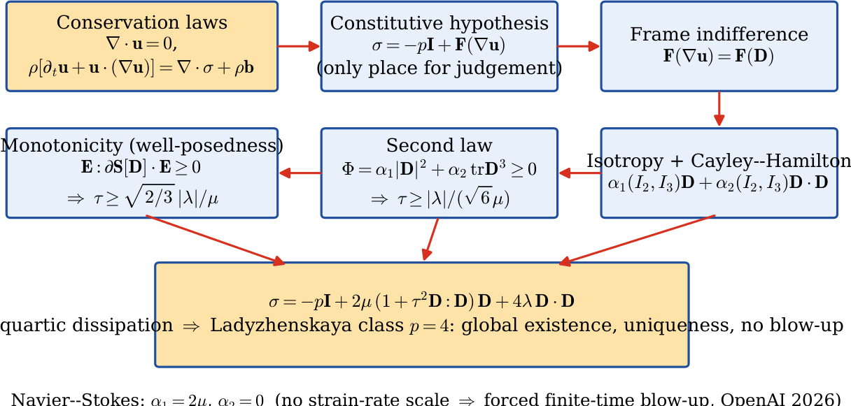
Figure 2.
(a) The plane. Below the second law is violated; between and the law is dissipative but the stress is not monotone and the equations are ill posed; above the theory is admissible and well posed. (b) Dissipation normalised by its Newtonian value along the extremal (axisymmetric straining) orientation of lemma 1, as a function of , for (the constant-coefficient model), , and .
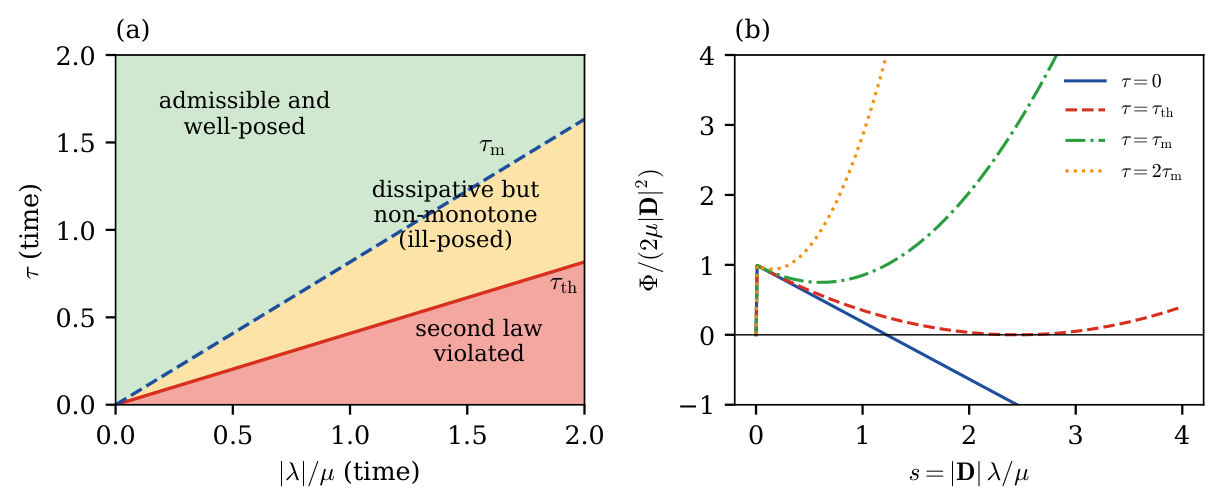
Figure 3.
Mechanism of the arrest of collapse. (a) Effective viscosity of the improved law compared with the constant Newtonian viscosity. (b) Relative magnitudes, in a collapsing core, of the inertial amplification , the Newtonian viscous stress , and the viscous stress of the improved law : the Newtonian stress is overtaken by the amplification, the improved stress is not.
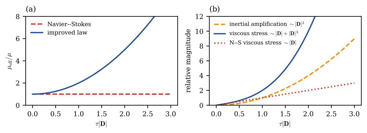
Figure 4.
Viscometric functions of the improved law in simple shear, with an arbitrary reference rate. (a) Shear stress for several values of . (b) Normal-stress differences: , .
Figure 4.
Viscometric functions of the improved law in simple shear, with an arbitrary reference rate. (a) Shear stress for several values of . (b) Normal-stress differences: , .
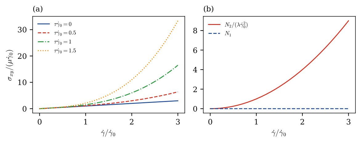
Figure 5.
Gravity-driven pipe flow. (a) Velocity profiles for (Poiseuille), , 1 and 3, normalised by the Poiseuille centre-line velocity. (b) Flow-rate ratio and wall shear rate as functions of , with the large- law . (c) Transverse pressure distribution in the vertical pipe for the same values of .
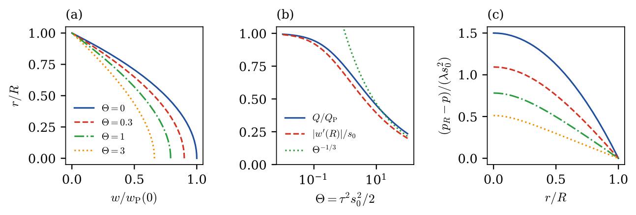
Figure 6.
The pipe experiment. Flow down a vertical pipe under gravity alone; the flow rate determines and the wall–axis pressure difference determines . The consistency condition and the rheometric cross-check provide two independent tests.
Figure 6.
The pipe experiment. Flow down a vertical pipe under gravity alone; the flow rate determines and the wall–axis pressure difference determines . The consistency condition and the rheometric cross-check provide two independent tests.
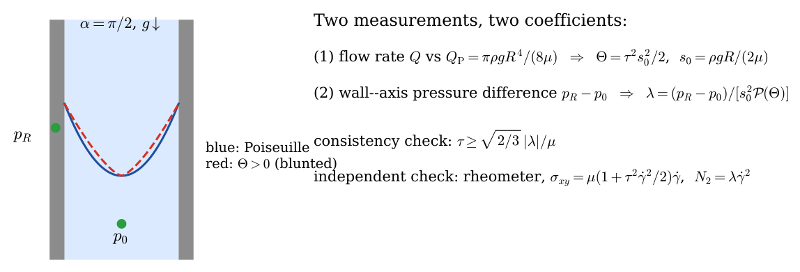
Figure 7.
The stiffened Burgers vortex, . (a) Azimuthal velocity and (b) vorticity for (Burgers), , and , with . (c) Peak vorticity as a function of , for and for , a value inside the admissible region of theorem 4.
Figure 7.
The stiffened Burgers vortex, . (a) Azimuthal velocity and (b) vorticity for (Burgers), , and , with . (c) Peak vorticity as a function of , for and for , a value inside the admissible region of theorem 4.
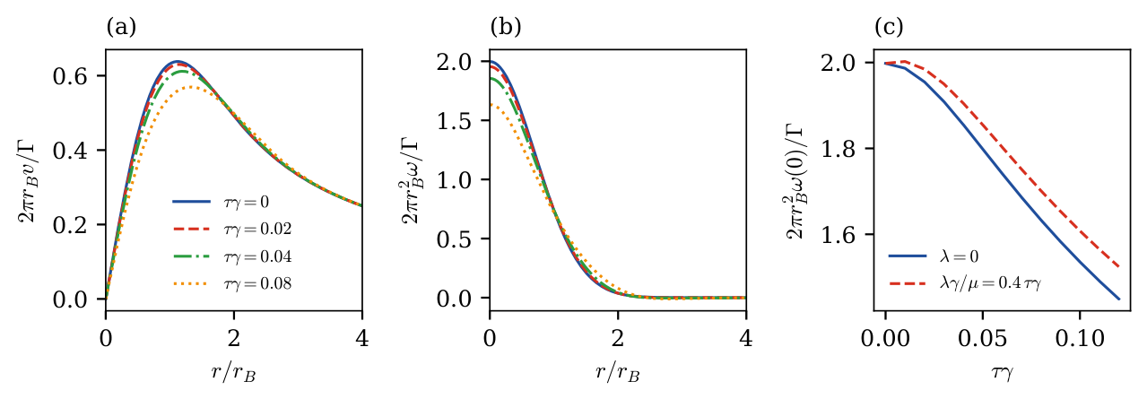
Figure 8.
Structure of the flat-plate boundary layer of the improved law. Upstream of the material length the wall shear rate exceeds , the fluid is shear-stiffened, and with ; downstream the layer relaxes to Blasius scaling, , . Velocity profiles are fuller in the stiffened regime.
Figure 8.
Structure of the flat-plate boundary layer of the improved law. Upstream of the material length the wall shear rate exceeds , the fluid is shear-stiffened, and with ; downstream the layer relaxes to Blasius scaling, , . Velocity profiles are fuller in the stiffened regime.
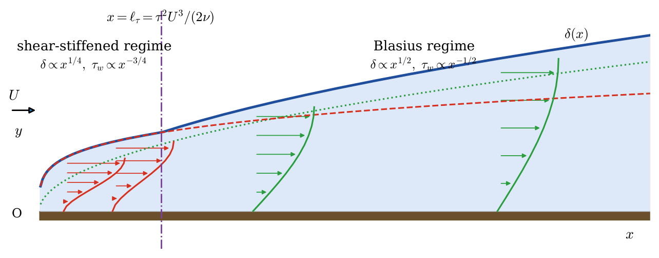
Figure 9.
Non-similar flat-plate solution. (a) Velocity profiles at , scaled by the local 99% thickness; the profiles become fuller as the leading edge is approached. (b) Skin-friction function against X, with the Blasius value and the leading-edge law (83). (c) Displacement and 99% thicknesses.
Figure 9.
Non-similar flat-plate solution. (a) Velocity profiles at , scaled by the local 99% thickness; the profiles become fuller as the leading edge is approached. (b) Skin-friction function against X, with the Blasius value and the leading-edge law (83). (c) Displacement and 99% thicknesses.
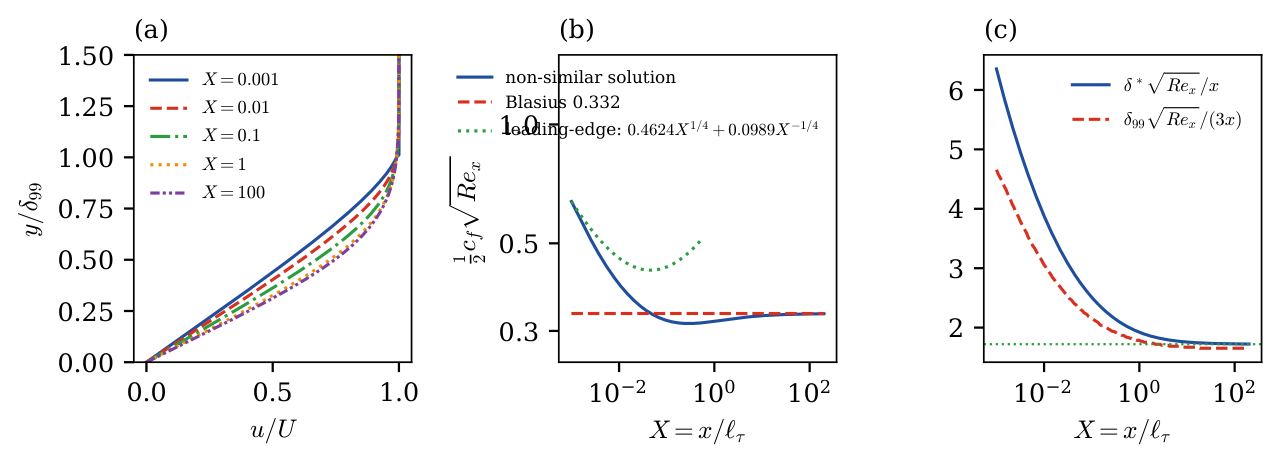
Figure 10.
The self-similar wedge boundary layer for . (a) Velocity profiles ; (b) . The profiles become fuller and the wall curvature smaller as grows, while the wall stress (Table 3) increases.
Figure 10.
The self-similar wedge boundary layer for . (a) Velocity profiles ; (b) . The profiles become fuller and the wall curvature smaller as grows, while the wall stress (Table 3) increases.
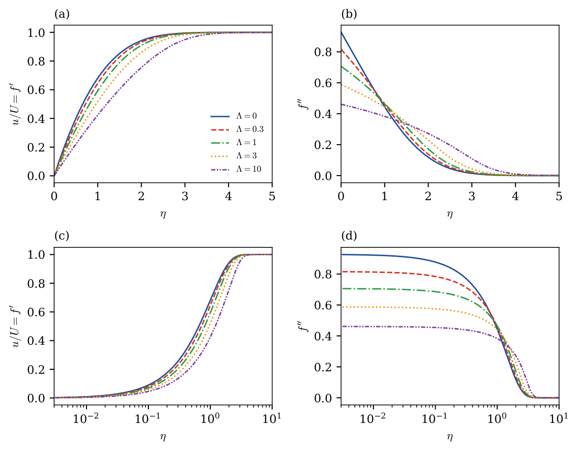

Table 1.
Flat-plate boundary layer of the improved law: wall value of , skin-friction function, displacement and 99% thicknesses, and total drag coefficient of a plate of length L, as functions of (or ).
Table 1.
Flat-plate boundary layer of the improved law: wall value of , skin-friction function, displacement and 99% thicknesses, and total drag coefficient of a plate of length L, as functions of (or ).
| for | |||||
|---|---|---|---|---|---|
| 0.0822 | 0.6381 | 6.355 | 13.97 | 4.671 | |
| 0.1370 | 0.3944 | 3.879 | 9.17 | 2.777 | |
| 0.2169 | 0.3189 | 2.511 | 6.46 | 1.810 | |
| 0.2560 | 0.3133 | 2.160 | 5.81 | 1.563 | |
| 1 | 0.2924 | 0.3174 | 1.922 | 5.36 | 1.434 |
| 3 | 0.3127 | 0.3231 | 1.814 | 5.11 | 1.355 |
| 10 | 0.3245 | 0.3279 | 1.756 | 5.01 | 1.341 |
| 100 | 0.3310 | 0.3313 | 1.726 | 4.96 | 1.328 |
| Blasius | 0.3321 | 0.3321 | 1.721 | 4.91 | 1.328 |
Table 2.
Gravity-driven pipe flow: flow rate, centre-line velocity and wall shear rate relative to Poiseuille values, and the pressure function of (66), as functions of .
Table 2.
Gravity-driven pipe flow: flow rate, centre-line velocity and wall shear rate relative to Poiseuille values, and the pressure function of (66), as functions of .
| 0 | 1.0000 | 1.0000 | 1.0000 | 1.5000 | 1.000 |
| 0.1 | 0.9448 | 0.9578 | 0.9217 | 1.3085 | 0.872 |
| 0.3 | 0.8724 | 0.8999 | 0.8291 | 1.0934 | 0.729 |
| 1 | 0.7438 | 0.7907 | 0.6823 | 0.7817 | 0.521 |
| 3 | 0.6020 | 0.6609 | 0.5366 | 0.5123 | 0.342 |
| 10 | 0.4513 | 0.5123 | 0.3930 | 0.2928 | 0.195 |
Table 3.
The self-similar wedge boundary layer (86): wall curvature of the stream function, wall shear-stress function and displacement thickness as functions of . The wall shear stress is , independent of x: it is uniform along the wall.
Table 3.
The self-similar wedge boundary layer (86): wall curvature of the stream function, wall shear-stress function and displacement thickness as functions of . The wall shear stress is , independent of x: it is uniform along the wall.
| 0 | 0.9277 | 0.9277 | 0.8046 |
| 0.05 | 0.9013 | 0.9379 | 0.8162 |
| 0.1 | 0.8793 | 0.9473 | 0.8267 |
| 0.2 | 0.8441 | 0.9643 | 0.8456 |
| 0.3 | 0.8163 | 0.9795 | 0.8623 |
| 0.5 | 0.7742 | 1.0062 | 0.8910 |
| 0.7 | 0.7426 | 1.0293 | 0.9157 |
| 1 | 0.7067 | 1.0595 | 0.9474 |
| 1.5 | 0.6636 | 1.1019 | 0.9914 |
| 2 | 0.6322 | 1.1377 | 1.0282 |
| 3 | 0.5878 | 1.1970 | 1.0886 |
| 5 | 0.5326 | 1.2882 | 1.1801 |
| 10 | 0.4615 | 1.4446 | 1.3350 |
Disclaimer/Publisher’s Note: The statements, opinions and data contained in all publications are solely those of the individual author(s) and contributor(s) and not of MDPI and/or the editor(s). MDPI and/or the editor(s) disclaim responsibility for any injury to people or property resulting from any ideas, methods, instructions or products referred to in the content. |
© 2026 by the author. Licensee MDPI, Basel, Switzerland. This article is an open access article distributed under the terms and conditions of the Creative Commons Attribution (CC BY) license.
Copyright: This open access article is published under a Creative Commons CC BY 4.0 license, which permit the free download, distribution, and reuse, provided that the author and preprint are cited in any reuse.