
Submitted:
13 August 2026
Posted:
16 September 2026
You are already at the latest version
Abstract
Weed interference is one of the main yield constraints in sugarcane (Saccharum spp.), andsite-specific management depends on identifying infested areas accurately and at low cost.This paper describes an end-to-end pipeline for weed segmentation in sugarcane from un-manned aerial vehicle (UAV) orthomosaics. Annotation is semi-automatic: operator-drawnbounding boxes prompt the Segment Anything Model 2 (SAM 2) to produce binary masks,which are then vectorised and exported as georeferenced GeoJSON. Two encoder–decodersegmentation models, built on VGG16 and MobileNetV2 encoders, were trained on 5,000tiles cropped from those orthomosaics under identical early stopping, checkpointing, and L2regularisation. Evaluated over approximately 6.9 million labelled pixels across four classes— sugarcane canopy (background), narrow-leaf weeds, broadleaf weeds, and castor bean(Ricinus communis) — the VGG16 model reached 83.06% pixel accuracy and 0.692 meanintersection over union (mIoU), against 73.87% and 0.549 for MobileNetV2. Per-class anal-ysis shows that the dominant error is not confusion between weed types, which accountsfor 1.9% of the pixels belonging to those two classes in the VGG16 model, but confusionbetween weed patches and the surrounding sugarcane canopy: broadleaf weeds lose 25.0%of their pixels to background, and 15.9% of background pixels are assigned to a weed class.Because the two models were trained on different colour representations, we report thecomparison as an operational baseline rather than a controlled architectural benchmarkand state explicitly what that confounding does and does not permit.
Keywords:
precision agriculture
; weed detection
; sugarcane
; semantic segmentation
; con-volutional neural networks
; UAV remote sensing
; Segment Anything Model
1. Introduction
Weeds compete with sugarcane for water, nutrients, light, and space, and the resulting interference translates directly into lost yield. Field experiments in Brazilian sugarcane have quantified this: infestations dominated by Brachiaria decumbens reduced stalk yield by up to 82%, and mixed infestations of signalgrass and guineagrass caused reductions near 40% [1]. The same body of work established that interference is concentrated in a critical window early in the cycle [2], which is precisely the period in which a grower benefits most from knowing where the infestation is rather than simply that it exists.
Uniform herbicide application ignores that spatial structure. It treats clean and infested areas alike, raising input costs and selection pressure for resistance without a corresponding yield benefit. Site-specific management is the alternative, but it presupposes a map, and producing that map by scouting is slow and does not scale to the field sizes typical of commercial sugarcane.
Automated identification from imagery is difficult for reasons specific to this crop. Sugarcane and many of its associated weeds are grasses; they share colour and coarse texture, so the discrimination is a green-on-green problem in which spectral thresholds and hand-designed features perform poorly. Morphology varies with growth stage, illumination changes across a flight, and weed patches merge visually into the canopy that surrounds them. Convolutional neural networks (CNNs) address this by learning discriminative representations directly from data, and they have become the dominant approach in crop–weed recognition [3]. dos Santos Ferreira et al. [4] demonstrated the principle in Brazilian soybean using UAV imagery, and Verçosa [5] applied CNNs specifically to weed detection in sugarcane.
A practical obstacle remains upstream of the model: supervised segmentation needs pixel-level labels, and producing them by hand over orthomosaics covering hundreds of hectares is prohibitive. Promptable segmentation models change this economics. The Segment Anything Model [6] and its successor SAM 2 [7] generate high-quality masks from cheap prompts such as points or boxes, which allows an operator to supply a bounding box in seconds and obtain a mask that would otherwise take minutes to trace.
This paper reports a pipeline built around that idea and evaluated on commercial sugarcane fields. Our contributions are:
- 1.
- a semi-automatic annotation workflow in which operator bounding boxes prompt SAM 2, and the resulting masks are georeferenced and exported as GeoJSON so that predictions remain tied to field coordinates;
- 2.
- a dataset of 5000 tiles cropped from UAV orthomosaics of commercial sugarcane, annotated at pixel level across agronomically defined weed categories;
- 3.
- a per-class evaluation over approximately 6.9 million pixels showing that the limiting error in this task is the weed–canopy boundary rather than discrimination among weed types—a finding that contradicts the intuition that morphologically similar weed groups are the hard case.
2. Related Work
- Weed recognition with deep learning.
Adhinata et al. [3] survey machine learning and deep learning for weed and crop classification and identify the recurring difficulties: visual similarity between weed and crop, occlusion, illumination variability, and the need for early-stage detection when plants are small and least distinctive. Among applications in Brazilian agriculture, dos Santos Ferreira et al. [4] combined SLIC superpixel segmentation with CNN classification on UAV soybean imagery, separating soil, crop, grass, and broadleaf weeds. Work specific to sugarcane is comparatively sparse; Verçosa [5] developed a CNN-based detector for weeds in sugarcane fields and reported that image quality and class diversity dominate performance.
- Semantic segmentation.
Fully convolutional networks [8] established dense prediction by replacing fully connected layers with convolutions and upsampling. U-Net [9] added skip connections between a contracting encoder and an expanding decoder, recovering the spatial detail lost to pooling; it remains a strong default when annotated data are limited, which is the usual situation in agriculture. Garcia-Garcia et al. [10] review the field more broadly.
- Backbone architectures.
VGG16 [11] stacks small convolutions into a deep, uniform network; its roughly 138 million parameters make it expensive, but its features transfer well. MobileNetV2 [12] uses depthwise separable convolutions with inverted residuals and linear bottlenecks to reach about 3.4 million parameters, targeting devices with limited compute. EfficientNet [13] later formalised the trade-off through compound scaling. In agricultural deployment the choice matters because inference may run on an embedded platform in a sprayer rather than on a workstation.
- Promptable segmentation for annotation.
SAM [6] introduced promptable segmentation trained on a billion-mask corpus, achieving strong zero-shot transfer. SAM 2 [7] extends the architecture with streaming memory and improves both accuracy and speed on images. Using such a model as an annotation accelerator, rather than as the deployed predictor, is the role it plays here.
- Loss functions for imbalanced segmentation.
Cross-entropy weights every pixel equally and therefore under-serves small structures. Region-overlap losses respond to this: Dice loss [14] optimises overlap directly, Tversky loss [15] adds asymmetric control over false positives and negatives, focal Tversky loss [16] concentrates gradient on hard examples, and focal loss [17] addresses the analogous imbalance in dense detection.
3. Materials and Methods
3.1. Image Acquisition and Dataset Construction
The imagery consists of orthomosaics assembled from UAV flights over commercial sugarcane fields. The aircraft carried a high-resolution RGB sensor; the resulting mosaics capture both healthy stands and infested areas, and each retains its geographic referencing so that any derived product can be mapped back to field coordinates. From these orthomosaics we cropped 5000 tiles.
Five categories were annotated, following the groups agronomists use when prescribing control (Figure 1):
- Sugarcane canopy (background)—healthy stand with no relevant infestation;
- Narrow-leaf weeds—grasses (Poaceae) morphologically close to the crop;
- Broadleaf weeds—dicotyledonous species with wide leaf blades;
- Castor bean (Ricinus communis)—treated separately because of its distinctive palmate leaf and its agronomic importance in the region;
- Other creeping weeds—prostrate species not covered by the categories above.
Separating narrow-leaf from broadleaf weeds is not a taxonomic formality: the two groups respond to different herbicide classes, so the distinction is what makes a prediction actionable.
The models reported in Section 4 were trained and evaluated on the first four of these categories. The other creeping weeds class was heterogeneous by construction—it was defined residually, as whatever the other four did not cover—and excluding it removed a source of label noise without changing the agronomic decision the system supports, since creeping species are treated with the same broad-spectrum products as the broadleaf group. All results below are therefore four-class.
3.2. Semi-Automatic Annotation with SAM 2
Pixel-level annotation was produced through the four-step procedure summarised in Figure 2.
- 1.
- Prompting. An operator draws bounding boxes around the elements of interest in a tile. Boxes are colour-coded, and the operator does not trace outlines—a coarse box is sufficient.
- 2.
- Mask generation. The boxes are passed to SAM 2 [7] as prompts. The model returns a binary mask per prompted region.
- 3.
- Polarity convention. For weed classes, foreground (white) denotes the weed. For background tiles, which contain only healthy sugarcane, the operator marks the regions that are not of interest and the mask is inverted, so that white consistently denotes the class named by the tile label.
- 4.
- Georeferencing and export. Mask contours are vectorised and written to GeoJSON, preserving the geographic coordinates inherited from the orthomosaic. Masks, source tiles, and GeoJSON files are stored together.
Every mask was inspected. Where SAM 2 produced an unsatisfactory boundary, the prompt was redrawn and the mask regenerated; ambiguous cases were referred to an agronomist. No mask entered the training set without approval.
3.3. Network Architectures
Both models follow an encoder–decoder design in the style of U-Net [9], differing only in the encoder (Table 1). Encoders were initialised from ImageNet [18] and fine-tuned rather than frozen. VGG16 [11] was chosen for its representational capacity and reliable transfer; MobileNetV2 [12] for its suitability to embedded inference.
3.4. Training Configuration
Table 2 lists the hyperparameters. Learning rates in the range to are conservative, which is appropriate when fine-tuning pretrained weights on a comparatively small dataset; Smith [19] discusses the sensitivity of training to this choice.
Three mechanisms guard against overfitting. Early stopping halts training when validation loss stops improving, which Prechelt [20] analyses as an implicit capacity constraint. Checkpointing retains the best validation state rather than the final one. regularisation penalises large weights [21]; the theoretical background for all three is treated in Goodfellow et al. [22].
The colour-space difference in the last row of Table 2 is not a controlled variable but a property of the two configurations as they were run. It is a confounder, and Section 5.4 states what follows from that.
3.5. Loss Functions
Three losses were evaluated (Table 3). Dice loss performed best and was used for the reported models, which is consistent with the class-imbalance argument: weed pixels are a minority of every tile, and a loss that optimises region overlap is less easily dominated by the majority class than pixel-wise cross-entropy.
3.6. Evaluation Protocol and Metrics
The dataset was partitioned into training, validation, and test subsets. Validation guided early stopping and checkpointing; the test subset was used once, for the figures reported in Section 4.
Evaluation is at pixel level. Writing , , and for the true positive, false positive, and false negative pixel counts of class c, we report
together with overall pixel accuracy and the frequency-weighted IoU, which weights by the share of ground-truth pixels in class c. Overall accuracy is reported for continuity with earlier work but should not be read alone: with background accounting for 62.4% of all pixels, a model that simply predicted background everywhere would already score above 0.6.
4. Results
Both models were evaluated over approximately labelled pixels.1
4.1. VGG16
The VGG16 model reached 83.06% overall pixel accuracy and 0.692 mIoU (Table 4). Per-class results are given in Table 5 and the confusion structure in Figure 3a.
Narrow-leaf weeds were the strongest class (, ) and broadleaf weeds the weakest (, ). The reason is visible in Figure 3a: 25.0% of broadleaf pixels were assigned to background, and 7.5% of background pixels were assigned to broadleaf. Castor bean shows the same asymmetry in the opposite direction—its recall is high (84.8%) but its precision is only 0.712, because 8.0% of the much larger background class was predicted as castor bean.
Confusion between weed types is minor. Only 2.6% of narrow-leaf pixels were labelled broadleaf and 1.6% of broadleaf pixels labelled narrow-leaf. The limiting factor is not telling weeds apart; it is telling weeds from the canopy they sit in.
The loss curves (Figure 4a) fall steeply over the first epochs and flatten around the sixth; early stopping triggered at epoch 10, with training loss ending near 0.47 and validation loss near 0.67.
4.2. MobileNetV2
The MobileNetV2 model reached 73.87% accuracy and 0.549 mIoU. Its error pattern differs from VGG16’s in an important way. Narrow-leaf weeds, the strongest class for VGG16, are its weakest (, ), driven by low precision (0.559): 7.8% of background pixels were predicted as narrow-leaf, and because background is roughly six times larger than the narrow-leaf class, that small percentage overwhelms the true positives.
Background recall fell to 71.5%, against 84.1% for VGG16. In operational terms this is the more consequential figure: 28.5% of clean canopy was assigned to some weed class, which in a variable-rate prescription would mean spraying more than a quarter of the uninfested area.
Training ran 19 epochs before early stopping, with training loss ending near 0.28 and validation loss near 0.45 (Figure 4b).
4.3. Comparison
VGG16 leads on every aggregate metric: 9.19 percentage points of pixel accuracy, 0.143 of mIoU, and 0.106 of mean . It also leads on all four classes individually, by margins ranging from 0.058 for castor bean to 0.259 for narrow-leaf. MobileNetV2 uses roughly 2.5% of the parameters.
Three clarifications matter for reading these numbers.
First, the final loss values are not comparable across the two runs. MobileNetV2 ends at a lower validation loss (0.45) than VGG16 (0.67) while segmenting substantially worse. Loss magnitude depends on the configuration that produced it, and comparing absolute values across runs that differ in input representation says nothing about segmentation quality. The IoU and figures, which are computed on the same label space, are the comparable quantities.
Second, epochs are not compute. VGG16 requires substantially more arithmetic per forward pass than MobileNetV2, so reaching its stopping criterion in fewer epochs does not mean it trained faster in wall-clock or energy terms, and it does not make it cheaper to deploy.
Third, reducing input channels does not make VGG16 efficient. Moving from three channels to one affects only the first convolutional layer; it does not meaningfully reduce the cost of a 138-million-parameter network. Any claim that grayscale input made VGG16 computationally competitive with MobileNetV2 would be unsupported, and we do not make it.
5. Discussion
5.1. The Limiting Error Is the Weed–Canopy Boundary
The per-class analysis overturns the intuition that guided the class design. Narrow-leaf and broadleaf weeds were separated as distinct categories on the assumption that telling them apart would be the hard problem, since both are green vegetation seen from above and the two groups are morphologically closer to each other than to bare soil. In the VGG16 model, that confusion accounts for 2.6% and 1.6% of the respective classes—close to negligible.
What dominates instead is confusion with background. Of the 1 168 899 misclassified pixels in the VGG16 model, 1 104 104, or 94.5%, involve background on one side or the other. This is what a green-on-green problem looks like at pixel level: the network can tell a broad leaf from a grass blade, but it cannot reliably decide where a weed patch ends and the sugarcane canopy begins. Boundary pixels are intrinsically ambiguous—leaves overlap, shadows fall across both—and they are also where annotation itself is least certain.
This reframes what would improve the system. Higher-capacity weed classifiers address a problem that is largely solved here. Better boundary delineation—higher ground sample distance, boundary-aware loss terms, or multispectral bands that separate species spectrally where RGB cannot—addresses the problem that actually binds.
5.2. Operational Reading
Which error is costly depends on the decision the map feeds. For a variable-rate sprayer, background recall is close to a direct measure of wasted input: every clean pixel called a weed is area sprayed unnecessarily. VGG16’s 84.1% against MobileNetV2’s 71.5% is therefore the difference between spraying about 16% and about 28% of clean canopy, which bears directly on whether the system delivers the input saving that motivates it.
Conversely, weed recall bounds the infestation that escapes treatment. Both models recover roughly 72–73% of broadleaf pixels, so approximately one broadleaf pixel in four would go untreated under either. Given that interference is concentrated early in the cycle [2], that residue is not negligible, and it is the figure we would want to improve before field deployment.
5.3. The Annotation Pipeline
The component we expect to transfer most readily is the annotation workflow. Prompting SAM 2 with a coarse box replaces manual contour tracing, and because the exported GeoJSON retains geographic coordinates, a prediction remains a location in a field rather than a label on an image. That property is what connects the model to a prescription map. The approach is not specific to sugarcane and should apply to any crop where pixel-level annotation cost is the bottleneck.
5.4. Limitations
The architecture comparison is confounded. VGG16 was trained on grayscale input and MobileNetV2 on RGB. Architecture and colour space vary together, so the differences in Table 4 cannot be attributed to architecture alone. Colour is plausibly informative for distinguishing vegetation types, so the direction of the confound is not obvious a priori—if anything, the RGB model had the representational advantage and still performed worse, but that observation is not a substitute for the experiment. Resolving this requires training both architectures on both representations.
Single split, no repetitions. Results come from one train/validation/test partition and one training run per configuration. Without cross-validation or repeated seeds we cannot separate a genuine difference from run-to-run variance, and none of the reported gaps carries a confidence interval. The partitions were also not pixel-identical between the two models.
Class exclusion. The other creeping weeds category was annotated but excluded from the reported experiments. Performance on the full five-class problem is therefore unknown, and the reported figures are optimistic relative to it.
Narrow geographic and temporal scope. All imagery comes from one production region, one crop cycle, and one sensor configuration. Generalisation to other regions, varieties, growth stages, and illumination conditions is untested.
Labels inherit SAM 2’s behaviour. Although every mask was reviewed, the boundaries originate from a model. Any systematic bias in how SAM 2 delineates vegetation edges would be inherited by the labels and therefore by the trained networks—and since the weed–canopy boundary is precisely where the models fail, this limitation and the main finding are not independent.
5.5. Future Work
The immediate priorities follow from the limitations: a factorial experiment crossing architecture with colour space, and k-fold cross-validation with repeated seeds on identical partitions. Beyond that, data augmentation [23] would address the limited sample size; encoders with better accuracy-per-FLOP such as EfficientNet [13] are worth evaluating for embedded inference; and given that the binding constraint is the weed–canopy boundary, boundary-aware losses and multispectral or near-infrared bands are the most promising directions. Validating predicted maps against ground-truth scouting, and quantifying the herbicide actually saved, is what would establish agronomic value rather than only segmentation performance.
6. Conclusions
We presented a pipeline for weed segmentation in sugarcane from UAV orthomosaics that couples SAM 2-assisted annotation with encoder–decoder CNNs over four agronomically defined classes. Evaluated on approximately 6.9 million labelled pixels, a VGG16-based model reached 83.06% pixel accuracy and 0.692 mIoU against 73.87% and 0.549 for MobileNetV2.
The per-class analysis carries the more useful result. Discriminating among weed types—the difficulty the class design anticipated—is close to solved, accounting for 1.9% of the pixels in those two classes in the better model. Over 94% of all errors involve the boundary between weed patches and the surrounding canopy. That is where the remaining accuracy lies, and it points at sensing and boundary modelling rather than at larger classifiers.
The annotation workflow is the component we consider most portable: promptable segmentation reduces the cost of pixel-level labelling enough to make supervised segmentation practical at field scale, and georeferenced GeoJSON output keeps predictions tied to coordinates a sprayer can act on. The architecture comparison, by contrast, is an operational observation rather than a controlled result, for the reasons given in Section 5.4; treating it otherwise would overstate what these experiments establish.
| 1 | The two evaluations cover slightly different pixel totals ( for VGG16 and for MobileNetV2, a difference of 0.14%). The partitions were therefore not pixel-identical, which is a further reason to treat the between-model difference as approximate. |
References
- Kuva, M.A.; Gravena, R.; Pitelli, R.A.; Christoffoleti, P.J.; Alves, P.L.C.A. Períodos de interferência das plantas daninhas na cultura da cana-de-açúcar: Iii – capim-braquiária (brachiaria decumbens) e capim-colonião (panicum maximum). Planta Daninha 2003, 21, 37–44. [Google Scholar] [CrossRef]
- Kuva, M.A.; Pitelli, R.A.; Christoffoleti, P.J.; Alves, P.L.C.A. Períodos de interferência das plantas daninhas na cultura da cana-de-açúcar: I – tiririca. Planta Daninha 2000, 18, 241–251. [Google Scholar] [CrossRef]
- Adhinata, F.D.; Wahyono; Sumiharto, R. A comprehensive survey on weed and crop classification using machine learning and deep learning. Artif. Intell. Agric. 2024, 13, 45–63. [Google Scholar] [CrossRef]
- dos Santos Ferreira, A.; Freitas, D.M.; da Silva, G.G.; Pistori, H.; Folhes, M.T. Weed detection in soybean crops using ConvNets. Comput. Electron. Agric. 2017, 143, 314–324. [Google Scholar] [CrossRef]
- dos Santos, V.J.P. Desenvolvimento de algoritmo baseado em redes neurais convolucionais para detecção de ervas daninhas em áreas de cana-de-açúcar. In Trabalho de Conclusão de Curso (Undergraduate Thesis); Arthur Costa Falcão, T., Ed.; Universidade Federal de Alagoas, Campus de Engenharias e Ciências Agrárias: Rio Largo, AL, Brazil, 2022; 60p, Available online: https://www.repositorio.ufal.br/handle/123456789/9876.
- Kirillov, A.; Mintun, E.; Ravi, N.; Mao, H.; Rolland, C.; Gustafson, L.; Xiao, T.; Whitehead, S.; Berg, A.C.; Lo, W.-Y. Segment anything. In Proceedings of the 2023 IEEE/CVF International Conference on Computer Vision (ICCV); IEEE: New York, NY, USA, 2023; pp. 3992–4003. [Google Scholar] [CrossRef]
- Ravi, N.; Gabeur, V.; Hu, Y.-T.; Hu, R.; Ryali, C.; Ma, T.; Khedr, H.; Rädle, R.; Rolland, C.; Gustafson, L. SAM 2: Segment anything in images and videos. arXiv 2024. Available online: https://arxiv.org/abs/2408.00714.
- Long, J.; Shelhamer, E.; Darrell, T. Fully convolutional networks for semantic segmentation. In Proceedings of the 2015 IEEE Conference on Computer Vision and Pattern Recognition (CVPR); IEEE: New York, NY, USA, 2015; pp. 3431–3440. [Google Scholar] [CrossRef]
- Ronneberger, O.; Fischer, P.; Brox, T. U-Net: Convolutional networks for biomedical image segmentation. In Medical Image Computing and Computer-Assisted Intervention—MICCAI 2015; Springer International Publishing: Cham, Switzerland, 2015; Volume 9351, pp. 234–241. ISBN 978-3-319-24574-4. [Google Scholar] [CrossRef]
- Garcia-Garcia, A.; Orts-Escolano, S.; Oprea, S.; Villena-Martinez, V.; Garcia-Rodriguez, J. A review on deep learning techniques applied to semantic segmentation. arXiv 2017. Available online: https://arxiv.org/abs/1704.06857.
- Simonyan, K.; Zisserman, A. Very deep convolutional networks for large-scale image recognition. In Proceedings of the 3rd International Conference on Learning Representations (ICLR), San Diego, CA, USA, 7–9 May 2015; Available online: https://arxiv.org/abs/1409.1556.
- Sandler, M.; Howard, A.; Zhu, M.; Zhmoginov, A.; Chen, L.-C. MobileNetV2: Inverted residuals and linear bottlenecks. In Proceedings of the 2018 IEEE/CVF Conference on Computer Vision and Pattern Recognition (CVPR); IEEE: New York, NY, USA, 2018; pp. 4510–4520. [Google Scholar] [CrossRef]
- Tan, M.; Le, Q.V. EfficientNet: Rethinking model scaling for convolutional neural networks. In Proceedings of the 36th International Conference on Machine Learning (ICML); Proceedings of Machine Learning Research: Cambridge, MA, USA, 2019; Volume 97, pp. 6105–6114. Available online: https://proceedings.mlr.press/v97/tan19a.html.
- Milletari, F.; Navab, N.; Ahmadi, S.-A. V-Net: Fully convolutional neural networks for volumetric medical image segmentation. In Proceedings of the 2016 Fourth International Conference on 3D Vision (3DV); IEEE: New York, NY, USA, 2016; pp. 565–571. [Google Scholar] [CrossRef]
- Salehi, S.S.M.; Erdogmus, D.; Gholipour, A. Tversky loss function for image segmentation using 3D fully convolutional deep networks. In Proceedings of the Machine Learning in Medical Imaging (MLMI 2017), Held with MICCAI 2017; Springer International Publishing: Cham, Switzerland, 2017; Volume 10541, pp. 379–387. ISBN 978-3-319-67389-9. [Google Scholar] [CrossRef]
- Abraham, N.; Khan, N.M. A novel focal Tversky loss function with improved attention U-Net for lesion segmentation. In Proceedings of the 2019 IEEE 16th International Symposium on Biomedical Imaging (ISBI 2019); IEEE: New York, NY, USA, 2019; pp. 683–687. [Google Scholar] [CrossRef]
- Lin, T.-Y.; Goyal, P.; Girshick, R.; He, K.; Dollár, P. Focal loss for dense object detection. IEEE Trans. Pattern Anal. Mach. Intell. 2020, 42, 318–327. [Google Scholar] [CrossRef] [PubMed]
- Deng, J.; Dong, W.; Socher, R.; Li, L.-J.; Li, K.; Fei-Fei, L. ImageNet: A large-scale hierarchical image database. In Proceedings of the 2009 IEEE Conference on Computer Vision and Pattern Recognition (CVPR); IEEE: New York, NY, USA, 2009; pp. 248–255. [Google Scholar] [CrossRef]
- Smith, L.N. Cyclical learning rates for training neural networks. In Proceedings of the 2017 IEEE Winter Conference on Applications of Computer Vision (WACV); IEEE: New York, NY, USA, 2017; pp. 464–472. [Google Scholar] [CrossRef]
- Prechelt, L. Early stopping—But when? In Neural Networks: Tricks of the Trade; Orr, G.B., Müller, K.-R., Eds.; Springer: Berlin/Heidelberg, Germany, 1998; Volume 1524, pp. 55–69. ISBN 978-3-540-49430-0. [Google Scholar] [CrossRef]
- Krogh, A.; Hertz, J.A. A simple weight decay can improve generalization. In Proceedings of the Advances in Neural Information Processing Systems 4 (NIPS 1991); Moody, J.E., Hanson, S.J., Lippmann, R.P., Eds.; Morgan Kaufmann: Burlington, MA, USA, 1991; Volume 4, pp. 950–957. Available online: https://papers.neurips.cc/paper/1991/hash/8eefcfdf5990e441f0fb6f3fad709e21-Abstract.html.
- Goodfellow, I.; Bengio, Y.; Courville, A. Deep Learning; Adaptive Computation and Machine Learning; MIT Press: Cambridge, MA, USA, 2016; ISBN 978-0-262-03561-3. [Google Scholar]
- Shorten, C.; Khoshgoftaar, T.M. A survey on image data augmentation for deep learning. J. Big Data 2019, 6, 60. [Google Scholar] [CrossRef]
Figure 1.
Representative tiles for the five annotated categories. In each panel the left image shows the input tile with operator box prompts and the right image shows the corresponding SAM 2 masks.
Figure 1.
Representative tiles for the five annotated categories. In each panel the left image shows the input tile with operator box prompts and the right image shows the corresponding SAM 2 masks.
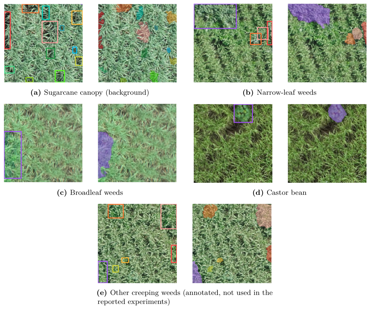
Figure 2.
Annotation pipeline. Step 1: operator-drawn bounding boxes on the input tile. Step 2: prompted regions after SAM 2 inference. Step 3: binary mask. Step 4: polarity-corrected mask for a background (sugarcane) tile, subsequently vectorised and exported to GeoJSON.
Figure 2.
Annotation pipeline. Step 1: operator-drawn bounding boxes on the input tile. Step 2: prompted regions after SAM 2 inference. Step 3: binary mask. Step 4: polarity-corrected mask for a background (sugarcane) tile, subsequently vectorised and exported to GeoJSON.
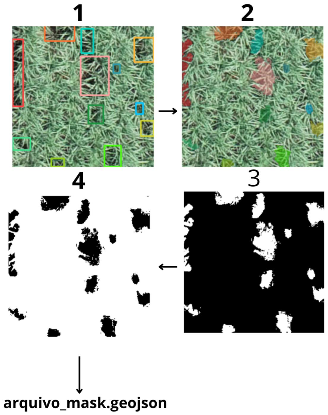
Figure 3.
Pixel-level confusion matrices, row-normalised. Each cell gives the percentage of the ground-truth class and the raw pixel count. In both models the off-diagonal mass concentrates in the background row and column rather than between the two weed-morphology classes.
Figure 3.
Pixel-level confusion matrices, row-normalised. Each cell gives the percentage of the ground-truth class and the raw pixel count. In both models the off-diagonal mass concentrates in the background row and column rather than between the two weed-morphology classes.
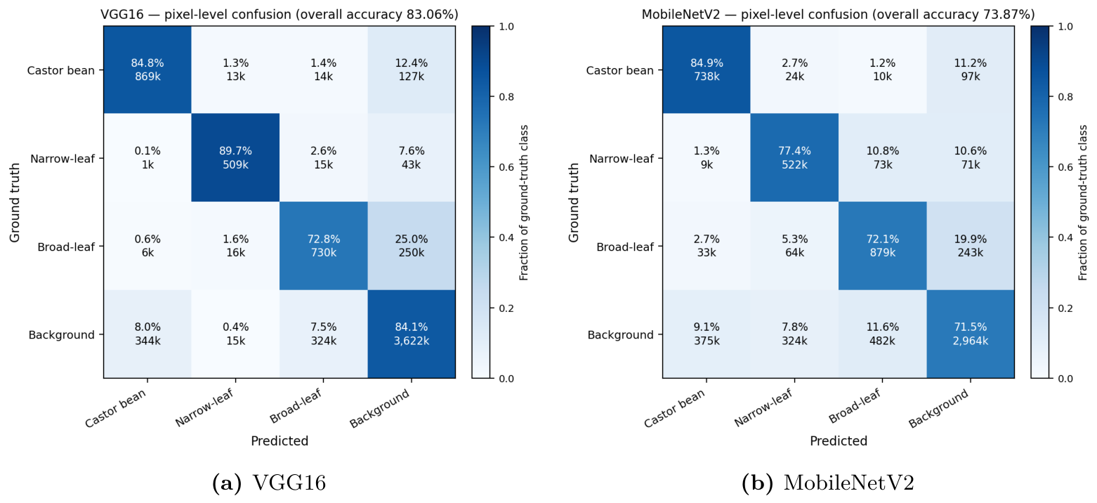
Figure 4.
Training and validation loss per epoch. The vertical scales differ between panels, and the absolute values are not comparable across the two configurations (Section 4).
Figure 4.
Training and validation loss per epoch. The vertical scales differ between panels, and the absolute values are not comparable across the two configurations (Section 4).
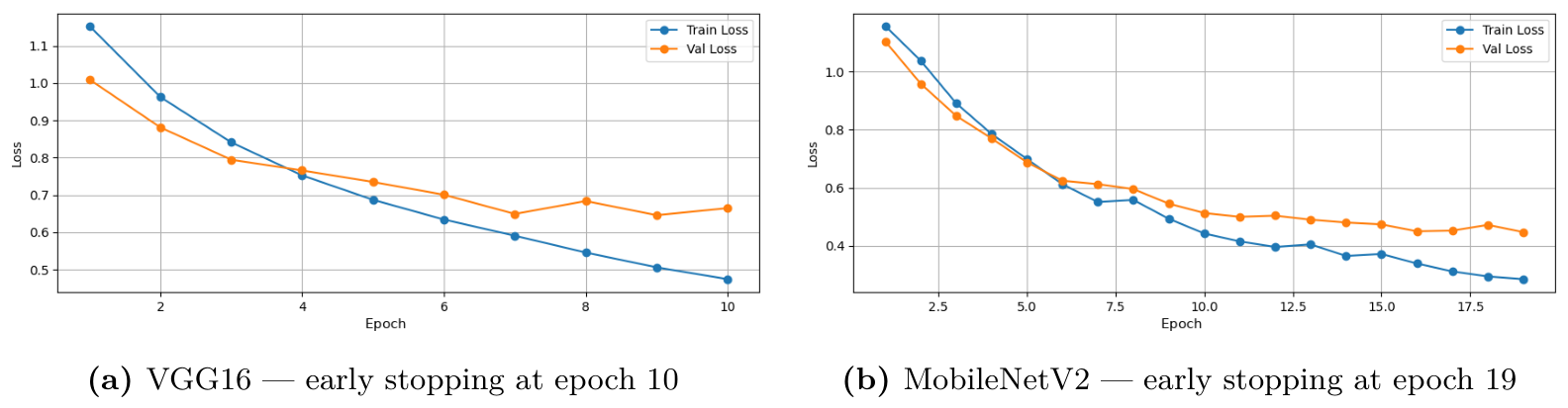

Table 1.
Encoder architectures evaluated.
| Encoder | Parameters | Rationale |
|---|---|---|
| VGG16 [11] | ≈138 M | Deep uniform stack of convolutions; high capacity and strong transfer, at high computational cost. |
| MobileNetV2 [12] | ≈3.4 M | Depthwise separable convolutions with inverted residuals; designed for resource-constrained inference. |
Table 2.
Hyperparameters and regularisation.
| Setting | Value |
|---|---|
| Learning rate | to |
| Batch size | 64 or 128 tiles |
| Early stopping | on validation loss; patience 3–4 epochs |
| Checkpointing | Weights saved whenever validation loss improved by at least |
| regularisation | Coefficient |
| Colour space | Grayscale (1 channel) for VGG16; RGB (3 channels) for MobileNetV2 |
Table 3.
Loss functions evaluated.
| Loss | Characteristics |
|---|---|
| Cross-entropy | Standard multi-class baseline; weights all pixels equally and is therefore sensitive to class imbalance. |
| Tversky [15] | Asymmetric weighting of false positives against false negatives; suited to imbalanced classes. |
| Dice [14] | Optimises region overlap directly; handled complex leaf boundaries best and was adopted. |
Table 4.
Aggregate results.
| Metric | VGG16 | MobileNetV2 |
|---|---|---|
| Overall pixel accuracy | 83.06% | 73.87% |
| Mean IoU | 0.692 | 0.549 |
| Frequency-weighted IoU | 0.719 | 0.596 |
| Mean | 0.813 | 0.707 |
| Epochs to early stopping | 10 | 19 |
| Evaluated pixels | 6 898 838 | 6 908 384 |
Table 5.
Per-class results, computed from the pixel-level confusion matrices in Figure 3.
Table 5.
Per-class results, computed from the pixel-level confusion matrices in Figure 3.
| VGG16 | MobileNetV2 | ||||||||
|---|---|---|---|---|---|---|---|---|---|
| Class | Support (px) | P | R | IoU | P | R | IoU | ||
| Castor bean | 1 024 335 | 0.712 | 0.848 | 0.775 | 0.632 | 0.639 | 0.849 | 0.729 | 0.574 |
| Narrow-leaf | 567 745 | 0.920 | 0.897 | 0.908 | 0.832 | 0.559 | 0.774 | 0.649 | 0.480 |
| Broadleaf | 1 001 561 | 0.674 | 0.728 | 0.700 | 0.539 | 0.609 | 0.721 | 0.660 | 0.493 |
| Background | 4 305 197 | 0.896 | 0.841 | 0.868 | 0.766 | 0.878 | 0.715 | 0.788 | 0.651 |
| Mean | 0.813 | 0.692 | 0.707 | 0.549 | |||||
Support is given for the VGG16 partition; the MobileNetV2 partition differs by 0.14% overall.
Disclaimer/Publisher’s Note: The statements, opinions and data contained in all publications are solely those of the individual author(s) and contributor(s) and not of MDPI and/or the editor(s). MDPI and/or the editor(s) disclaim responsibility for any injury to people or property resulting from any ideas, methods, instructions or products referred to in the content. |
© 2026 by the authors. Licensee MDPI, Basel, Switzerland. This article is an open access article distributed under the terms and conditions of the Creative Commons Attribution (CC BY) license (http://creativecommons.org/licenses/by/4.0/).
Copyright: This open access article is published under a Creative Commons CC BY 4.0 license, which permit the free download, distribution, and reuse, provided that the author and preprint are cited in any reuse.