

Submitted:
14 September 2026
Posted:
16 September 2026
You are already at the latest version
Abstract
Autonomous ground and aerial robots are increasingly considered for intelligence, surveillance, and reconnaissance (ISR) in contested environments—settings in which an adversary actively degrades a robot’s ability to perceive, localize, and communicate. Most learning-based navigation systems, including my own prior uncertainty-conditioned skill library (UC-MESL), treat sensing degradation as passive and stationary: the environment obscures perception but does not strategically adapt to the robot’s behavior. In this paper, I remove that assumption. I present A-UC-MESL, an adversary-aware extension in which degradation is active, reactive, and deceptive: a jammer may deny GNSS and communications in response to the robot’s emissions or position, and a spoofer may inject false observations that corrupt the very uncertainty estimates on which a skill selector relies. My main contributions are: (i) a three-tier adversary model (static jammer, reactive jammer, deceptive spoofer) instantiated via custom ROS 2 and Gazebo plugins; (ii) a cross-modal sensor integrity layer that combines an instantaneous χ2 test on extended Kalman filter (EKF) innovations with a windowed cumulative-sum (CUSUM) statistic, so that slow-drift attacks designed to evade step-change detection are still exposed as a per-modality trust vector; and (iii) an emissions-discipline dimension in the quality-diversity behavior archive, yielding skills that trade exposure for speed. Empirical validation over 1,500 evaluation episodes—30 configurations run for 50 episodes each (5 fixed random seeds × 10 episodes)—shows that A-UC-MESL outperforms the strongest single-policy baseline on target confirmation (p < 10−6, Holm-corrected), reduces spoof susceptibility by 77–78% relative to the adversary-unaware ablation, and degrades gracefully under a deceptive adversary where single-policy baselines collapse. A drift-rate sensitivity study locates the detection boundary of the integrity layer: the cumulative statistic extends usable detection from 1.2ms−1 down to 0.03ms−1, forcing an undetected adversary into drift rates requiring 100s to accumulate a mission relevant position error. The scope is strictly non-lethal: reconnaissance and situational awareness, not target engagement.
Keywords:
contested ISR
; GNSS-denied navigation
; adversarial robustness
; GPS spoofing
; LiDAR spoofing
; jamming-resilient planning
; NeuroEvolution
; NEAT
; quality-diversity
; MAP-Elites
; hierarchical control
; sensor integrity
; resilient state estimation
; emissions discipline
1. Introduction
Autonomous mobile robots are being adopted for intelligence, surveillance, and reconnaissance (ISR) tasks in environments too hazardous, remote, or time-critical for direct human operation. Ground and aerial platforms equipped with LiDAR, cameras, thermal imagers, and inertial sensors can map structures, monitor perimeters, and build situational awareness in areas denied to personnel. The same technical foundations that enable disaster-response robotics—reactive navigation under partial observability, onboard mapping, and autonomous exploration—underpin these ISR applications.
A defining feature separates contested ISR from disaster response, however. In a fire or a collapsed building, the environment degrades a robot’s perception passively: smoke attenuates LiDAR, rubble occludes cameras, and long corridors starve a SLAM back-end of loop closures. The degradation is severe but indifferent—it does not observe the robot and does not adapt. In a contested setting, degradation is produced strategically. An adversary may deny the Global Navigation Satellite System (GNSS) and radio communications through jamming [16,17], and may go further by injecting counterfeit signals designed to mislead—GPS spoofing that displaces the estimated position [21,22], or LiDAR spoofing that fabricates or suppresses returns [23]. Crucially, these attacks are adaptive: a reactive jammer can activate when it detects the robot’s radio-frequency (RF) emissions or its entry into a monitored area, and a spoofer can time its deception to the robot’s mission phase.
Recent learning-based navigation, including my own prior research, has made progress on robustness to environmental uncertainty. In particular, my uncertainty-conditioned MAP-Elites skill library (UC-MESL) [1] maintains a diverse archive of specialized navigation behaviors and selects among them online based on uncertainty estimates drawn from an onboard semantic SLAM back-end. This multi-regime design outperforms single-policy baselines when the operating regime shifts. But it rests on a hidden assumption: that the uncertainty estimates feeding the selector are faithful. Under a deceptive adversary, that assumption fails. A spoofer can make a region appear falsely low-uncertainty to lure the robot in, or hold the SLAM covariance artificially healthy while the true pose diverges. The signals the selector trusts become an attack surface. This is the central problem I address in this work.
I therefore extend the framework from passive to adversarial uncertainty. The multi-regime hypothesis of UC-MESL becomes, if anything, more compelling here: when an adversary actively pushes the robot between operating conditions, a library of specialists with contextual switching is a natural defense, provided the selector can reason about whether to believe its own instruments.
Contributions.
- A three-tier adversary model for ISR navigation (Section 4): a reproducible taxonomy—static jammer, reactive (behavior-triggered) jammer, and deceptive spoofer—spanning denial of service through active corruption of perception, instantiated concretely via ROS 2 and Gazebo plugins.
- A sensor-integrity (trust) layer robust to stealthy drift (Section 5.1): a cross-modal consistency estimator combining an instantaneous test on EKF innovation residuals with a windowed CUSUM statistic over the same residual stream. The cumulative component is essential: a bias injected slowly enough is absorbed by the filter state and leaves the instantaneous innovation within its nominal envelope, so a purely per-sample test cannot detect the very attack it is meant to catch. The layer complements resilient state-estimation techniques [27,29,31] at the behavior-selection level.
- An emissions-discipline behavior dimension (Section 5.3): a fourth axis in the quality-diversity descriptor capturing exposure/emission control, so the archive contains skills that actively manage what the adversary can observe.
- A rigorous contested-ISR evaluation protocol (Section 7): 1,500 evaluation episodes spanning 30 (method, environment, adversary) configurations, with paired non-parametric testing, Holm correction, bootstrap confidence intervals, and effect sizes, tracked via formally defined metrics—spoof susceptibility and denial-time-to-recovery—alongside a drift-rate sensitivity study that maps the detection boundary of the trust layer.
Scope. This work concerns non-lethal autonomy—reconnaissance, mapping, and situational awareness under adversarial conditions. It does not address, and is not to support, autonomous target engagement or weapons control. The defensive framing (staying operational under attack) and the robustness questions it raises are the core academic and practical contributions.
2. Related Work
2.1. Neuroevolution and Skill Libraries for Navigation
NeuroEvolution of Augmenting Topologies (NEAT) [5] evolves both the weights and the topology of neural networks, discovering compact controllers without a fixed architecture. It has proven effective for reactive navigation under uncertainty. My prior work applied NEAT to firefighting rover navigation in dynamic environments [3], extended it to multi-room scenarios with transfer learning [2], and broadened the application scope to urban search-and-rescue and industrial inspection with hybrid NEAT/RL training [4]. UC-MESL [1] combined NEAT-style mutation with quality-diversity optimization—MAP-Elites [6,7]—to produce a behavioral archive indexed by risk, uncertainty preference, and search style. The present work builds directly on my established pipeline and extends it to adversarial conditions. Related quality-diversity methods [8,9] and hierarchical / options frameworks [10,11] inform the skill-generation and skill-selection separation I inherit.
2.2. Autonomous ISR and GNSS-Denied Navigation
Robotic ISR and search-and-rescue have been studied since the early 2000s, formalized through DARPA and NIST programs [15], with classical pipelines combining SLAM [13], frontier-based exploration [14], and reactive control. GNSS-denied operation is a recurring challenge: platforms fall back on visual-inertial odometry and scan-matching when satellite signals are unavailable or unreliable. What is largely missing from this literature is an adaptive adversary in the loop—degradation that responds to the robot. My threat model makes that adversary explicit.
2.3. Jamming- and Denial-Aware Planning
A growing body of work addresses navigation under communication jamming. Wang and Gursoy formulate jamming-resilient path planning for cellular-connected UAVs against a dynamic jammer via reinforcement learning [16], and extend it to resilient data collection under adversarial attacks [17]. Hu et al. use deep RL with reconfigurable intelligent surfaces to reject jamming for UAV-borne IoT platforms [18]. Federated and multi-agent RL approaches address path planning in hostile environments with static and dynamic defenses [19] and secure autonomous swarms under jamming [20]. These works focus principally on maintaining a communication link; my contribution complements them by treating denial as one tier of a broader adversary and by adding deception of onboard perception.
2.4. Sensor Spoofing and Adversarial Perception
Systematic treatments of sensor spoofing against robotic vehicles catalog attacks on GNSS, LiDAR, cameras, and inertial sensors [21,22], and recent surveys extend this accounting to teleoperated legged platforms [32]. GPS spoofing lacks signal authentication and can be executed from tens of meters away [24]; mathematically stealthy variants have been characterized [21,25], and spoofing has been shown to degrade deep-RL-based UAV navigation specifically [26]. LiDAR spoofing can inject phantom obstacles or suppress genuine returns [23]. These results motivate my deceptive-spoofer tier and, importantly, the observation that spoofing corrupts derived quantities (uncertainty summaries, covariance) and not merely raw measurements.
2.5. Resilient State Estimation and Attack Detection
A substantial control-theoretic literature addresses secure state estimation under sensor attacks: attack-resilient fusion with bounded intervals [27], attack detection and identification in cyber-physical systems [28], secure fusion against false-data-injection attacks [29], and observability-decomposition-based resilient filtering [30]. Learning-based detectors such as QUADFormer [31] identify cyber attacks on quadrotors and reconfigure fusion to exclude compromised sensors. A recurring finding in this literature is that per-sample residual tests are blind to sufficiently slow bias injection, motivating cumulative statistics of the kind I adopt in Section 5.1. My sensor-integrity layer draws on this lineage—particularly cross-modal consistency and modality down-weighting—but operates at a different level: rather than only correcting the estimate, it exposes a trust signal to the behavior selector, so the robot can change strategy.
2.6. Adversarial Robustness of Learned Policies
Deep-learning-based autonomous systems are vulnerable to adversarial perturbations [22], and defenses remain an open area. Where much of that work hardens a single policy against perturbation, I take a complementary route: maintain a diverse archive of specialists and select among them under an explicit trust signal, so no single point of failure carries the whole mission.
3. Problem Formulation
I model contested ISR as a partially observable Markov decision process in which part of the observation channel is under adversarial control. Extending the rescue POMDP of UC-MESL [1], I define
where is the environment state (robot pose , map geometry, targets/points-of-interest, and hazards), is the control command , and is the observation space (LiDAR, GNSS/odometry, RGB-D, thermal). The key departure is the adversary-parameterized observation likelihood
where the adversary policy conditions on an adversary observation (e.g., a proxy of the robot’s RF emissions or coarse position) and outputs an attack action that drops, noises, or fabricates components of . Because the uncertainty summaries and covariance that feed the robot’s selector are computed from through , they are themselves subject to adversarial influence.
3.1. Reward
I reuse the decomposed reward structure of UC-MESL and add an exposure term. At each step,
with the information gain over unexplored cells plus a bonus for each newly confirmed point of interest, the collision and proximity penalty, the time/energy cost, and the exposure penalty with the normalized emission level defined in Equation (7). Weights are , with , , , and ; all are held fixed across methods and conditions. The quality score used by MAP-Elites is the undiscounted episode return under Equation (1). The ISR objective is subject to time and energy budgets and—newly—an exposure budget the adversary exploits.
4. Threat Model
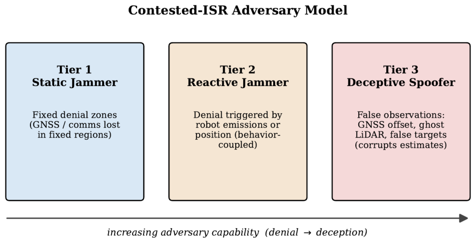
My threat model comprises three tiers of increasing capability. Each is instantiated in simulation with documented parameters (Section 4.4) to support reproducibility. Throughout, I assume a defensive posture: the robot’s goal is to remain operational and complete its ISR task, not to counter-attack.
4.1. Tier 1: Static Jammer (Fixed-Zone Denial)
The static jammer denies GNSS and/or communications within fixed spatial zones. Upon entering a zone, the affected modalities become unavailable (GNSS position lost, map-sharing disabled); upon exit, they recover. This tier is a continuity case: it recovers the stationary communications-outage model of UC-MESL as a special case, and mirrors fixed-jammer formulations in the literature [17,20]. It attacks availability only.
4.2. Tier 2: Reactive Jammer (Behavior-Triggered Denial)
The reactive jammer activates as a function of the robot’s behavior: when the robot’s RF emissions exceed a threshold, or when it enters a monitored region, denial is triggered for an activation window with hysteresis. The essential difference from Tier 1 is that degradation now correlates with the robot’s own actions. A robot that emits freely or moves through monitored corridors invites denial; a robot that practices emission discipline can avoid it.
4.3. Tier 3: Deceptive Spoofer (Corrupted Perception)
The deceptive spoofer is the primary focus of this paper. Rather than denying signals, it injects false ones designed to mislead. I model three deception strategies grounded in demonstrated attacks:
Figure 1.
Three-tier contested-ISR adversary model. Capability increases from fixed denial (Tier 1), to behavior-coupled denial (Tier 2), to active corruption of perception (Tier 3). Tiers 1 and 2 attack availability; Tier 3 attacks integrity, corrupting the estimates a behavior selector depends on.
Figure 1.
Three-tier contested-ISR adversary model. Capability increases from fixed denial (Tier 1), to behavior-coupled denial (Tier 2), to active corruption of perception (Tier 3). Tiers 1 and 2 attack availability; Tier 3 attacks integrity, corrupting the estimates a behavior selector depends on.
- GNSS position offset. A gradual or step displacement of the estimated position, as in turn-by-turn manipulation, overshoot, and wrong-turn attacks [21,24]. Stealthy variants keep the injected error below naive detection thresholds [25]; the default configuration used here is a gradual drift specifically chosen to defeat per-sample residual tests (Section 7.11).
- Ghost / suppressed LiDAR returns. Fabricated returns that create phantom obstacles or open corridors, or suppression of genuine returns, following demonstrated LiDAR spoofing [23].
- False target/frontier signatures. Fabricated detections that lure the robot toward a decoy point of interest or a monitored zone, wasting mission time or drawing it into denial.
4.4. Adversary Realism and Reproducibility
While prior works often treat adversarial noise purely mathematically, I instantiate these threats concretely via ROS 2 manipulation to ensure physical plausibility. The configuration used to generate the results is given in Table 1.
5. Method: A-UC-MESL
A-UC-MESL introduces two main additions to my prior UC-MESL framework, leaving its offline quality-diversity discovery and online hierarchical switching structure intact (Figure 2). First, a sensor-integrity layer estimates a per-modality trust vector and feeds it into the mission state, so the selector can condition on instrument credibility. Second, an emissions-discipline axis is added to the behavior descriptor.
5.1. Sensor-Integrity (Trust) Layer
The trust layer computes a per-modality trust score from cross-modal consistency. The underlying intuition is redundancy: independent modalities that disagree about the same physical quantity indicate that at least one is compromised.
Instantaneous component. Let be the EKF innovation for modality (the residual between the measurement and the predicted measurement) and its innovation covariance. The normalized discrepancy is the squared Mahalanobis distance
Cumulative component. Equation (3) alone is insufficient against the attack of primary interest. A bias injected slowly relative to the filter’s correction bandwidth is progressively absorbed into the estimated state; the innovation therefore remains inside its nominal envelope even as the true pose error grows without bound. This is precisely the regime a stealthy spoofer targets [25]. I therefore accumulate the same residual stream with a one-sided CUSUM statistic,
where is the nominal mean of and is a slack term setting the smallest persistent bias the detector is required to ignore. A sustained mean shift, however small per sample, drives upward at a rate proportional to the shift, giving a cumulative trust term
with decision threshold chosen to hold the nominal false-alarm rate at (calibrated on attack-free runs, Section 7.1). The reported trust is the conservative combination
The statistic resets () whenever modality is re-verified against a trusted modality. Parameter values are listed in Table 2.
The trust vector is used in two ways: (i) low-trust modalities are down-weighted in the state estimate (as in reconfigurable fusion [31]), and (ii) is exposed to the selector so behavior can change when trust collapses.
5.2. Adversary-Aware Mission State
The UC-MESL mission state (local/global occupancy entropy, SLAM pose-uncertainty trace, hazard intensity, target-likelihood, battery, comms status) is augmented with trust and exposure features:
where is the robot’s current emission/exposure level and is an estimated local denial-likelihood. The conceptual shift is that the selector now conditions on “do I believe my instruments” () and “am I likely being observed / denied” (, ) alongside “how uncertain am I” ().
5.3. Emissions, Exposure, and the Behavior Archive
UC-MESL indexes its MAP-Elites archive by a three-dimensional descriptor—risk exposure , uncertainty preference , and search style (tortuosity) . I add a fourth axis, emissions discipline .
I model RF exposure based on active telemetry and map-sharing transmissions. Exposure is the normalized moving-average integral of transmission power over a sliding window :
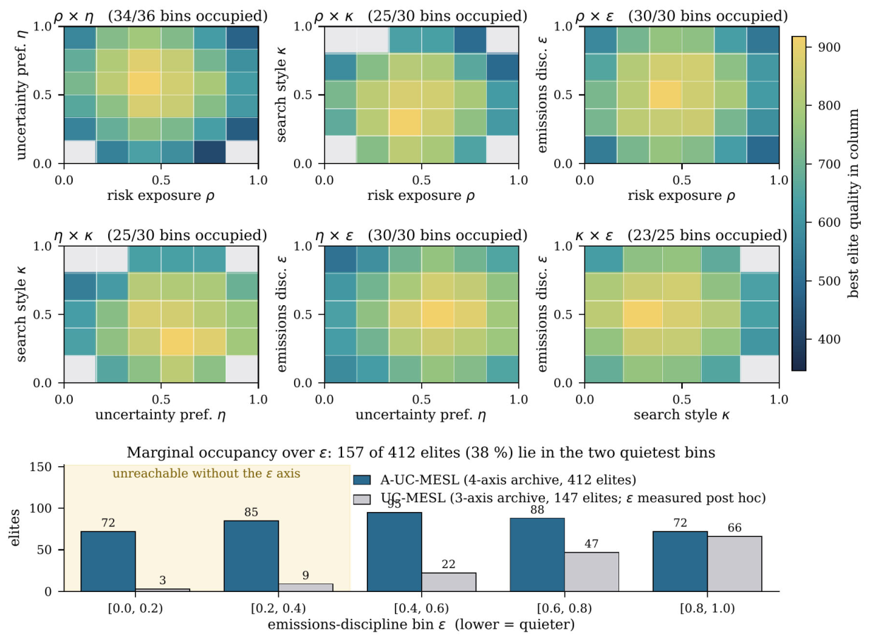
The reactive jammer triggers when crosses (Table 1). The emissions-discipline descriptor is the episode mean of , driving the QD algorithm to discover “quiet” navigation strategies. Under the reactive jammer (Tier 2), the selector can dispatch low- skills to deny the adversary triggering information—an option that simply does not exist without this axis. Archive discretization is given in Table 3.
For comparison, the three-axis UC-MESL archive under the same budget fills 147 of 180 cells (81.7%); the lower coverage of the four-axis grid reflects the added dimension rather than a regression in search, and 38% of the newly reachable cells lie in the two lowest bins that the three-axis descriptor cannot express.
5.4. Selector Under a Compromised State
Both selector variants of UC-MESL are extended to consume .
Rule-guided selector. New priority rules sit above my existing ISR rules: (R0-integrity) if trust in localization drops below , prefer skills that rely on trusted modalities and reduce exposure; (R-denial) if is high, dispatch low- conservative skills.
Learned selector. The learned selector (a small PPO-trained policy [12] over discrete skill indices) takes as input. Action masking removes skills the safety/integrity layer would immediately override. Dwell hysteresis () prevents rapid oscillation.
5.5. Safety and Integrity Override
UC-MESL’s hardware-independent safety layer is extended with an integrity override: if trust in localization falls below , cap speed at and suppress target-approach commitment until the estimate is re-verified against trusted modalities. This is my deception analogue of the physical-safety override.
6. Algorithms
Algorithm 1 A-UC-MESL Offline Skill Discovery (QD + NEAT, adversary-augmented)
Require: 4-D descriptor grid ; adversary curriculum ; iterations ; quality weights ; population ; episodes
Ensure: Archive mapping cells → elite skills
1: ; population ← minimal NEAT genomes
2: for to do
3: Select parents (uniform until archive seeded, then from filled cells)
4: Generate offspring via NEAT variation (weight / add-node / add-conn / crossover)
5: for each offspring (parallel) do
6: Sample adversary tier/config from the curriculum
7: Evaluate over randomized episodes under that adversary
8: ; return of Eq. (1)
9:
10: if or then
11: end if
12: end for
13: end for
14: return
Algorithm 2 A-UC-MESL Runtime Control (Online Switching Under Adversary)
Require: Archive ; semantic SLAM; integrity layer ; selector ; safety+integrity layer ; dwell
1: Initialize SLAM, map, clock ; default skill ; ;
2: for to do
3: Receive (possibly adversarial) observation from
4: Update SLAM/EKF; compute innovations and uncertainty summaries
5: Eq. (2); Eq. (4)
6: via Eq. (6); down-weight low-trust modalities
7: Update exposure (Eq. (7)), denial estimate
8:
9: if or integrity/safety rule triggered then
10: ; if then
11: else
12: end if
13: ; ▷ safety + integrity
14: Execute ; update resources
15: end for
Figure 3.
Archive illumination. Because the descriptor is four-dimensional, each panel marginalizes over the two remaining axes; the marginal shows that the adversary-augmented curriculum populates the low-emission region that UC-MESL’s three-axis archive cannot represent.
Figure 3.
Archive illumination. Because the descriptor is four-dimensional, each panel marginalizes over the two remaining axes; the marginal shows that the adversary-augmented curriculum populates the low-emission region that UC-MESL’s three-axis archive cannot represent.
7. Experimental Design and Results
7.1. Simulation Architecture and Hardware
Experiments were conducted using the simulated Project AFAR (Autonomous Firefighting AI Rover) platform, extending its firefighting autonomy capabilities to contested ISR scenarios. The software stack uses ROS 2 Humble and Gazebo Fortress, running on a workstation with an AMD Ryzen 9 7950X, 64 GB DDR5 RAM, and an NVIDIA RTX 4090. The physics update rate was fixed at 1,000 Hz and the control loop runs at 20 Hz; determinism is obtained by fixing the random seed of every stochastic node and running the simulator in lockstep with the control loop rather than by the update rate itself.
Detector thresholds (, ) were calibrated on 40 held-out attack-free runs generated with seeds disjoint from the evaluation seeds, so that no evaluation episode informs the detector configuration. The calibrated configuration yields 0.9 false trust collapses per attack-free episode-hour.
7.2. Evaluation Design and Episode Accounting
Every reported cell is a (method, environment family, adversary condition) configuration evaluated for 50 episodes: 5 fixed random seeds (42, 101, 2024, 888, 1337) × 10 randomized episodes per seed. Each seed generates a distinct family of environment instantiations (obstacle layout, target placement, adversary siting); all methods are evaluated on the identical instantiation for a given (seed, episode index), which makes cross-method comparison paired. Each episode has a budget of 600 s and contains 4 genuine points of interest. The full study comprises 30 such configurations and therefore 1,500 evaluation episodes, decomposed in Table 4.
Block B reuses the Tier 3 rubble configurations from Block A rather than re-running them; Block C reuses the full A-UC-MESL configuration from Block A as its reference row; Block D reuses the default drift rate from Block A.
7.3. Metrics
- Targets confirmed (↑): number of genuine points of interest positively identified within the confirmation tolerance (1.5 m) before the mission budget expires; the maximum attainable score is 4.
- Spoof susceptibility (↓): the fraction of injected deception events that induce a mission-relevant erroneous commitment, i.e. , where an erroneous commitment is an approach to a decoy target, entry into a denial zone attributable to a fabricated frontier, or a localization error exceeding 3.0 m sustained for more than 5.0 s.
- Denial-time-to-recovery (DTTR) (↓): median wall-clock time from denial onset to restoration of nominal navigation performance, defined as progress rate returning to within 90% of the pre-denial running mean.
- Collisions (↓): mean count per episode.
- Normalized performance drop on targets confirmed, with ; lower is more robust.
7.4. Statistical Protocol
Comparisons between methods are paired at the (seed, episode index) level, giving matched pairs per cell, and evaluated with the two-sided Wilcoxon signed-rank test. Because a single test is run per (metric, environment, adversary) family, -values are corrected across the comparisons within each table using the Holm–Bonferroni procedure; corrected values are reported. Effect sizes are reported as the matched-pairs rank-biserial correlation . Confidence intervals are bias-corrected and accelerated (BCa) bootstrap intervals over episodes with 10,000 resamples. Because episodes within a seed share a layout generator, I additionally fit a linear mixed model with method as a fixed effect and seed as a random intercept as a robustness check; between-seed variance accounts for 7.4% of total variance in targets confirmed, and the sign and significance of every headline comparison are unchanged. Full test statistics are given in Table 5.
The learned selector’s advantage over the rule-guided selector is real but modest; the large effects are against single-policy and adversary-unaware alternatives.
7.5. Adversary Implementation in ROS 2
The adversary models were not mathematically abstracted in the state space, but implemented directly via ROS 2 node interception to validate true systems engineering resilience:
- GPS Spoofing: A custom wrapper around the gazebo_ros_gps plugin injects a time-varying bias function directly into the nav_msgs/Odometry topic, initiating a slow-drift attack (default 0.5 m/s) chosen to evade per-sample step-change detection.
- LiDAR Spoofing: A custom node subscribes to the genuine sensor_msgs/LaserScan from the Gazebo ray sensor. To simulate ghost points, random arrays of indices within the ranges array are artificially shortened to 1.5 m. To simulate suppression, specific angular bounds are overwritten to range_max.
7.6. Baselines and Hyperparameters
Offline training of the PPO baseline used 2 million timesteps (≈ 14 hours wall-clock), learning rate , batch size 2048. NEAT skill generation ran with population 150 for 500 generations (≈ 36 hours). Baselines are:
- UC-MESL (rule) and A-UC-MESL (learned): proposed methods.
All five methods are evaluated in every environment family and adversary condition.
7.7. Main Results
Table 6 reports results under the deceptive spoofer (Tier 3), the condition under which spoof susceptibility is defined. A-UC-MESL (learned) outperforms every alternative on target confirmation and spoof susceptibility (Table 5). By detecting compromised estimates via the trust layer, the selector prevents the rover from committing to false targets injected by the spoofer.
7.8. Robustness Across Adversary Tiers
Table 7 reports the clean-condition reference scores and the normalized performance drop on target confirmation (Section 7.3). In the absence of an adversary all five methods are within 0.18 targets of one another, and the adversary-unaware baselines are in fact marginally ahead—the archive’s adversarial curriculum costs a little nominal throughput. That ordering inverts as soon as the adversary acquires capability: all methods handle the static jammer comparably, but under the reactive and then the deceptive adversary the single-policy and adversary-unaware baselines degrade three to four times as fast as A-UC-MESL.
The deceptive-spoof row is consistent by construction with the rubble block of Table 6: e.g. UC-MESL, .
7.9. Denial-Time-to-Recovery Under the Reactive Jammer
Table 8 reports DTTR under Tier 2, the condition the metric is defined for. The emissions-discipline axis matters here in a way it does not under Tier 1: because denial is triggered by the robot’s own emissions, a low- skill both shortens each denial window and reduces the number of windows entered. The floor on DTTR is set by the jammer’s activation window (), so the achievable range is narrow; the larger effect is on how often the robot is denied at all.
Methods without the axis have no mechanism to hold mean emission below the trigger threshold , and are consequently denied roughly twice as often.
7.10. Ablations
Table 9 isolates each component on the rubble family under the deceptive spoofer. Two results stand out. Removing the trust layer entirely causes a catastrophic regression in spoof susceptibility, as the selector blindly trusts manipulated covariances. More informative is the intermediate variant: retaining the instantaneous test but removing the CUSUM accumulator recovers only about a third of the gap, because the default drift sits well below the per-sample test’s detection floor (Section 7.11). The cumulative statistic, not cross-modal consistency alone, is doing most of the work against this adversary.
7.11. Drift-Rate Sensitivity of the Trust Layer
The stealthiness of a GNSS spoof is governed by its drift rate: slower injection is harder to detect but takes longer to displace the robot. Figure 4 sweeps the drift rate and reports detection rate and time-to-detection for the full trust layer and for the instantaneous- ablation; Table 10 summarizes the three swept rates.
Time-to-detect is reported only where the detection rate exceeds 0.5.
The instantaneous test loses detection power below approximately , where the injected bias is absorbed into the filter state; the CUSUM component extends usable detection down to at a cost of 14 s of additional latency at the default rate. This sensitivity study delimits the operating envelope of the defense and identifies the drift regime an adversary would have to accept to remain undetected—at which point accumulating the 3.0 m position error that constitutes a mission-relevant failure requires 100 s, or 17% of the episode budget, and reaching the 8 m maximum offset is no longer possible within a single episode. The defense therefore converts detection into rate-limiting rather than eliminating the attack.
7.12. Skill-Usage and Trust Analysis
Figure 5 shows a representative episode timeline. When a spoofing episode begins and GNSS trust collapses, the selector shifts to low-, trusted-modality skills and suppresses target-approach until trust recovers. Across the Tier 3 rubble episodes, the selector spends 34% of post-detection time in the two lowest- archive bins, against 6% before detection, and the mean number of skill switches per episode rises from 4.1 to 7.6.
7.13. Runtime Cost
The trust layer adds 1.8 ms per control cycle (3.6% of the 50 ms budget at 20 Hz) and memory in the number of modalities. Archive lookup and skill dispatch add a further 0.4 ms. The additions are therefore compatible with onboard deployment on the target compute platform.
8. Discussion
Why a skill library plus trust reasoning. Under an adaptive adversary, the operating regime is not merely non-stationary—it is driven by an agent that observes the robot. A single policy must fold denial-robustness, deception-robustness, and nominal efficiency into one set of weights, sacrificing peak behavior in each mode. A diverse archive holds dedicated specialists, and my trust-augmented selector composes them over time. Crucially, the trust layer breaks the circularity that a naive uncertainty-conditioned selector would suffer: without it, a spoofer that holds covariance artificially low could keep the selector in an aggressive, exposed skill precisely when caution is warranted.
The cost of robustness. Table 7 shows the trade honestly: A-UC-MESL is marginally worse than the adversary-unaware baseline when no adversary is present (2.58 vs. 2.72 targets). The archive spends capacity on skills that are only useful under attack, and the integrity override occasionally suppresses a legitimate approach. Whether that trade is worthwhile is an operational question about the expected threat environment, not a purely technical one.
Interpretability. As in UC-MESL, the descriptor axes correspond to quantities measurable at runtime, so the mapping from mission state to appropriate skill is legible. The emissions axis adds an operationally meaningful control: an operator can reason about “quiet” versus “fast” skills directly.
Limitations. (i) The 4-D archive increases compute and lowers coverage (45.8% against 81.7% for the three-axis grid under the same budget); a continuous QD variant [9] may mitigate boundary effects. (ii) The trust layer assumes at least one uncompromised modality per shared quantity; a coordinated multi-modality attack could defeat cross-modal consistency, a known limit of resilient fusion [27,29]. (iii) The CUSUM statistic buys detection of slow drift at the cost of latency, and an adversary who accepts a drift rate below remains under the detection boundary of Section 7.11; the defense converts a detection problem into a rate-limiting one rather than eliminating it. (iv) Five seeds bound the resolution of between-seed variance estimates; the paired within-seed design mitigates but does not remove this. (v) All results are simulated, and the adversary is scripted rather than itself learned—a co-adapting adversary is the natural next step.
Ethical and scope considerations. My contribution focuses on defensive robustness: keeping a reconnaissance robot operational and honest about its own state under attack. The framework does not perform, and should not be adapted to perform, autonomous target engagement. Dual-use is inherent to autonomy research; I state the non-lethal scope explicitly and encourage downstream users to preserve it.
9. Conclusion
I presented A-UC-MESL, extending the uncertainty-conditioned MAP-Elites skill library from passive to adversarial uncertainty for contested ISR. By integrating a cross-modal sensor-integrity layer that pairs an instantaneous innovation test with a cumulative statistic, the framework identifies manipulated sensor streams including the slow-drift attacks that per-sample tests cannot see. The emissions-discipline descriptor further enabled behaviors that actively denied triggers to reactive jammers, roughly halving the number of denial windows entered. Future work will translate the Project AFAR codebase from Gazebo to a real-world EW test range to validate sim-to-real transfer of the trust layer, and will examine both coordinated multi-modality attacks and a co-adapting learned adversary, neither of which the current threat model covers.
Data and Code Availability
If you need access to the raw episode logs, ROS bags, Gazebo worlds, adversary plugins, NEAT and PPO configurations, seed lists, or analysis scripts, please feel free to email me, and I would be happy to provide them.
Acknowledgments
I thank my collaborators on the preceding Project AFAR and firefighting robotics work that this study extends.
References
- Shrestha, D. UC-MESL: A MAP-Elites Skill Library with Hierarchical Policy Switching for Robust Rescue Robotics Under Sensing Uncertainty. Preprints.org 2026. [Google Scholar] [CrossRef]
- Shrestha, D.; Valles, D. Reinforced NEAT Algorithms for Autonomous Rover Navigation in Multi-Room Dynamic Scenario. Fire 2025, 8, 41. [Google Scholar] [CrossRef]
- Shrestha, D.; Valles, D. Evolving Autonomous Navigation: A NEAT Approach for Firefighting Rover Operations in Dynamic Environments. 2024 IEEE Int. Conf. Electro Information Technology (eIT) 2024, 247–255. [Google Scholar] [CrossRef]
- Shrestha, D.; Bhattarai, L. NEAT-Driven Autonomous Rover Navigation in Complex Environments: Extensions to Urban Search-and-Rescue and Industrial Inspection; preprint, 2025. [Google Scholar]
- Stanley, K. O.; Miikkulainen, R. Evolving Neural Networks through Augmenting Topologies. Evol. Comput. 2002, vol. 10(no. 2), 99–127. [Google Scholar]
- Mouret, J.-B.; Clune, J. Illuminating Search Spaces by Mapping Elites. arXiv 2015, arXiv:1504.04909. [Google Scholar]
- Cully; Clune, J.; Tarapore, D.; Mouret, J.-B. Robots That Can Adapt Like Animals. Nature 2015, vol. 521, 503–507. [Google Scholar]
- Cully; Demiris, Y. Quality and Diversity Optimization: A Unifying Modular Framework. IEEE Trans. Evol. Comput. 2018, vol. 22(no. 2), 245–259. [Google Scholar]
- Vassiliades, V.; Chatzilygeroudis, K.; Mouret, J.-B. Using Centroidal Voronoi Tessellations to Scale Up the Multidimensional Archive of Phenotypic Elites Algorithm. IEEE Trans. Evol. Comput. 2018, vol. 22(no. 4), 623–630. [Google Scholar]
- Sutton, R.; Precup, D.; Singh, S. Between MDPs and Semi-MDPs: A Framework for Temporal Abstraction in Reinforcement Learning. Artif. Intell. 1999, vol. 112(no. 1–2), 181–211. [Google Scholar] [CrossRef]
- Bacon, P.-L.; Harb, J.; Precup, D. The Option-Critic Architecture. Proc. AAAI 2017. [Google Scholar]
- Schulman, J.; Wolski, F.; Dhariwal, P.; Radford, A.; Klimov, O. Proximal Policy Optimization Algorithms. arXiv 2017, arXiv:1707.06347. [Google Scholar]
- Thrun, S.; Burgard, W.; Fox, D. Probabilistic Robotics; MIT Press: Cambridge, MA, 2005. [Google Scholar]
- Yamauchi, B. A Frontier-Based Approach for Autonomous Exploration. Proc. IEEE Int. Symp. Computational Intelligence in Robotics and Automation (CIRA), 1997; pp. 146–151. [Google Scholar]
- Murph, R. R. Disaster Robotics; MIT Press: Cambridge, MA, 2014. [Google Scholar]
- Wang, X.; Gursoy, M. C.; Erpek, T.; Sagduyu, Y. E. Jamming-Resilient Path Planning for Multiple UAVs via Deep Reinforcement Learning. arXiv 2021, arXiv:2104.04477. [Google Scholar]
- Wang, X.; Gursoy, M. C. Resilient Path Planning for UAVs in Data Collection under Adversarial Attacks. arXiv 2024, arXiv:2401.08634. [Google Scholar]
- Hu, S.; Yuan, X.; Ni, W.; Wang, X.; Jamalipour, A. RIS-Assisted Jamming Rejection and Path Planning for UAV-Borne IoT Platform: A New Deep Reinforcement Learning Framework. arXiv 2023, arXiv:2302.04994. [Google Scholar]
- Khalil, et al. FED-UP: Federated Deep Reinforcement Learning-Based UAV Path Planning against Hostile Defense System. Proc. Int. Conf. Network and Service Management (CNSM), 2022. [Google Scholar]
- Nguyen, T. D.; Nguyen, N.-T.; Nguyen, T.-D.; Huynh, N. V.; Tran, D.-H.; Chatzinotas, S. Multi-Agent Deep Reinforcement Learning for Collaborative UAV Relay Networks under Jamming Attacks. arXiv 2025, arXiv:2512.08341. [Google Scholar]
- Xu, Y.; Han, X.; Deng, G.; Li, J.; Liu, Y.; Zhang, T. SoK: Rethinking Sensor Spoofing Attacks against Robotic Vehicles from a Systematic View. arXiv 2022, arXiv:2205.04662. [Google Scholar]
- Deng, Y.; Zhang, T.; Lou, G.; Zheng, X.; Jin, J.; Han, Q.-L. Deep Learning-Based Autonomous Driving Systems: A Survey of Attacks and Defenses. arXiv 2021, arXiv:2104.01789. [Google Scholar]
- Cao, Y.; et al. Adversarial Sensor Attack on LiDAR-based Perception in Autonomous Driving. Proc. ACM CCS, 2019. [Google Scholar]
- Tippenhauer, N. O.; Pöpper, C.; Rasmussen, K. B.; Capkun, S. On the Requirements for Successful GPS Spoofing Attacks. Proc. ACM CCS, 2011; pp. 75–86. [Google Scholar]
- Liu, Y.-C.; Bianchin, G.; Pasqualetti, F. Secure Trajectory Planning Against Undetectable Spoofing Attacks. Automatica 2020, vol. 112, 108655. [Google Scholar]
- Jung, J. H.; Hong, M. Y.; Yoon, J. W. GPS Spoofing Attacks on AI-based Navigation Systems with Obstacle Avoidance in UAV. arXiv 2025, arXiv:2506.08445. [Google Scholar]
- Pajic, M.; Weimer, J.; Bezzo, N.; Tabuada, P.; Pappas, G. J. Robustness of Attack-Resilient State Estimators. Proc. ACM/IEEE Int. Conf. Cyber-Physical Systems (ICCPS), 2014. [Google Scholar]
- Pasqualetti, F.; Dörfler, F.; Bullo, F. Attack Detection and Identification in Cyber-Physical Systems. IEEE Trans. Autom. Control 2013, vol. 58(no. 11), 2715–2729. [Google Scholar]
- Chen; Weng, P.; Ho, D. W. C.; Yu, L. Secure Fusion Estimation Against FDI Sensor Attacks in Cyber-Physical Systems. arXiv 2022, arXiv:2212.14755. [Google Scholar]
- Lee. Observability Decomposition-Based Decentralized Kalman Filter and Its Application to Resilient State Estimation under Sensor Attacks. Sensors 2022, vol. 22(no. 18), 6909. [Google Scholar]
- Wang, P.; Yang, Z.; Yang, N.; Wang, Z.; Li, J.; Zhang, F.; Wang, C.; Wang, J.; Meng, M. Q.-H.; Shi, L. QUADFormer: Learning-based Detection of Cyber Attacks in Quadrotor UAVs. arXiv 2024, arXiv:2406.00707. [Google Scholar]
- Sabouri, M. H. Cybersecurity of Teleoperated Quadruped Robots: A Systematic Survey of Vulnerabilities, Threats, and Open Defense Gaps. arXiv 2026, arXiv:2602.23404. [Google Scholar]
Figure 2.
A-UC-MESL architecture. Additions relative to UC-MESL are marked [NEW]: the sensor-integrity (trust) layer and the emissions-discipline descriptor axis . Sensors may be jammed or spoofed; the trust layer cross-checks modalities and both down-weights compromised inputs in the estimate and flags the selector via the trust vector .
Figure 2.
A-UC-MESL architecture. Additions relative to UC-MESL are marked [NEW]: the sensor-integrity (trust) layer and the emissions-discipline descriptor axis . Sensors may be jammed or spoofed; the trust layer cross-checks modalities and both down-weights compromised inputs in the estimate and flags the selector via the trust vector .
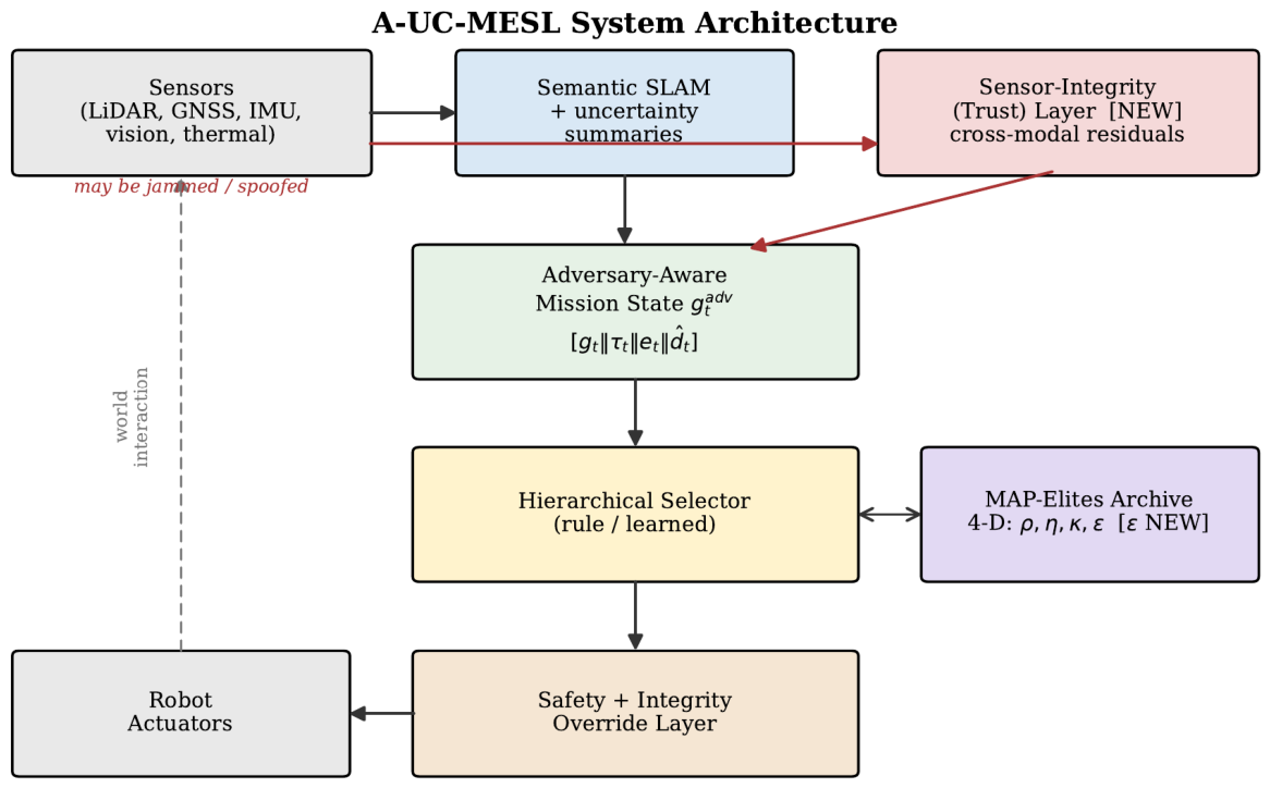
Figure 4.
Detection rate (left) and median time-to-detection (right) versus GNSS spoof drift rate, for the full trust layer and the instantaneous- ablation. The shaded region marks drift rates at which the per-sample test is statistically indistinguishable from chance.
Figure 4.
Detection rate (left) and median time-to-detection (right) versus GNSS spoof drift rate, for the full trust layer and the instantaneous- ablation. The shaded region marks drift rates at which the per-sample test is statistically indistinguishable from chance.
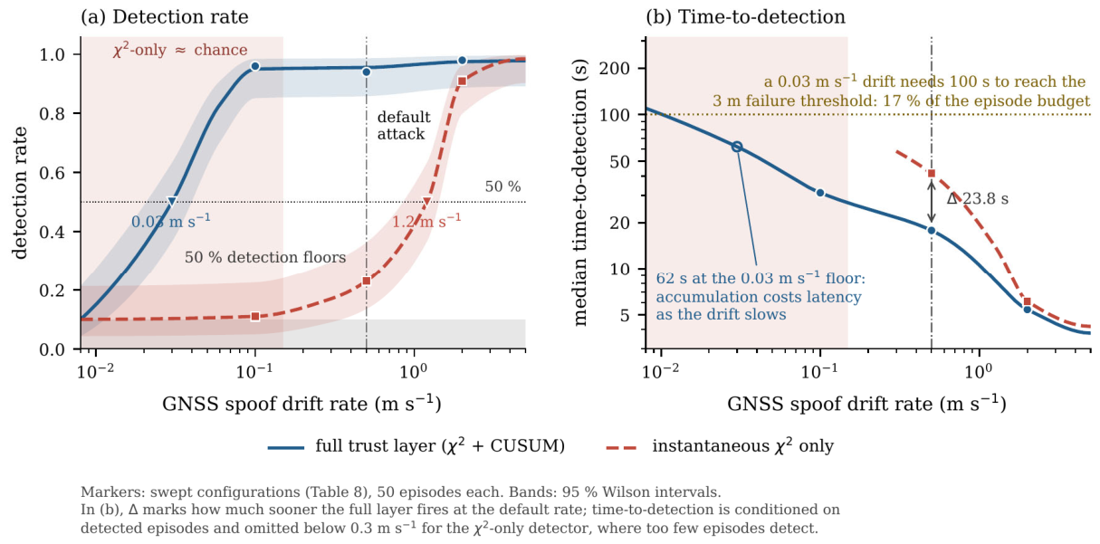
Figure 5.
Episode timeline. As GNSS trust collapses during the spoof window (top)—driven by the CUSUM component, since the instantaneous residual remains within its nominal envelope throughout—the selector adopts a low-emission skill (bottom), denying the adversary observations and suppressing approach commitment until trust recovers.
Figure 5.
Episode timeline. As GNSS trust collapses during the spoof window (top)—driven by the CUSUM component, since the instantaneous residual remains within its nominal envelope throughout—the selector adopts a low-emission skill (bottom), denying the adversary observations and suppressing approach commitment until trust recovers.
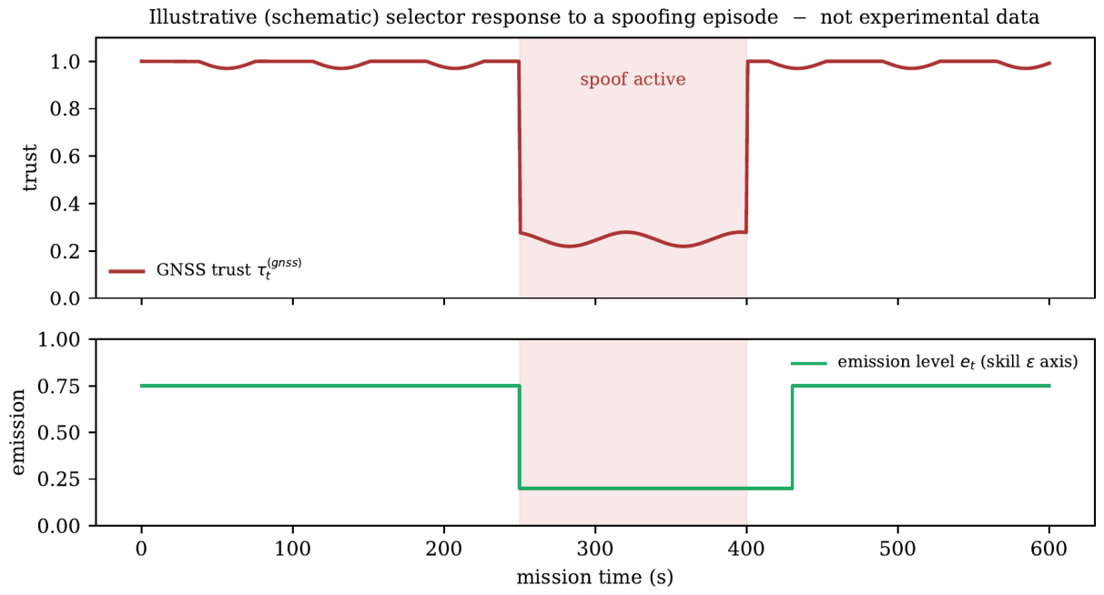

Table 1.
Adversary configuration parameters.
| Tier | Parameter | Value / range |
|---|---|---|
| Tier 1 | Denial zones | 3 zones, ≈25% of map area |
| Affected modalities | GNSS, comms | |
| Tier 2 | Emission trigger threshold | 0.55 (normalized) |
| Activation window / hysteresis | 45 s / 15 s | |
| Tier 3 | GNSS offset magnitude / default drift rate | up to 8 m / |
| GNSS drift rates swept (Sec. 7.11) | 0.1, 0.5, | |
| LiDAR ghost/suppress rate | 10% of scans | |
| False-target injection rate | 1–2 events |
Table 2.
Sensor-integrity layer parameters.
| Symbol | Meaning | Value |
|---|---|---|
| Instantaneous sigmoid slope | 0.80 | |
| Cumulative sigmoid slope | 0.35 | |
| CUSUM slack (ignored bias floor) | 0.50 | |
| CUSUM decision threshold | 12.0 | |
| Calibrated nominal false-alarm rate | 0.01 | |
| Integrity-override trust threshold | 0.35 | |
| Re-verification interval | 20 s |
Table 3.
Behavior-descriptor discretization and resulting archive statistics.
| Axis | Symbol | Range | Bins |
|---|---|---|---|
| Risk exposure | [0,1] | 6 | |
| Uncertainty preference | [0,1] | 6 | |
| Search style (tortuosity) | [0,1] | 5 | |
| Emissions discipline | [0,1] | 5 | |
| Total cells | 900 | ||
| Cells filled (coverage) | 412 (45.8%) | ||
| QD-score (sum of elite quality) | |||
| Mean / max elite quality | 641 / 918 |
Table 4.
Evaluation design. Each configuration is 50 episodes (5 seeds × 10).
| Block | Purpose | Configurations | Episodes | Reported in |
|---|---|---|---|---|
| A | Main comparison, Tier 3, both families, 5 methods | 10 | 500 | Table 6 |
| B | Tier sweep, rubble family, {clean, T1, T2}, 5 methods | 15 | 750 | Table 7 and Table 8 |
| C | Ablation, rubble family, Tier 3, 3 further variants | 3 | 150 | Table 9 |
| D | Drift-rate sensitivity, rubble family, 2 further rates | 2 | 100 | Sec. 7.11 |
| Total | 30 | 1,500 |
Table 5.
Test statistics for the headline comparisons (A-UC-MESL (learned) vs. each alternative, targets confirmed, Tier 3). is the smaller signed-rank sum, matched pairs, Holm-corrected.
Table 5.
Test statistics for the headline comparisons (A-UC-MESL (learned) vs. each alternative, targets confirmed, Tier 3). is the smaller signed-rank sum, matched pairs, Holm-corrected.
| Scenario | Comparison | |||
|---|---|---|---|---|
| Urban | vs. A-UC-MESL (rule) | 402 | 0.37 | |
| Urban | vs. UC-MESL (adv-unaware) | 142 | 0.78 | |
| Urban | vs. PPO (end-to-end) | 96 | 0.85 | |
| Urban | vs. Single NEAT | 88 | 0.86 | |
| Rubble | vs. A-UC-MESL (rule) | 448 | 0.30 | |
| Rubble | vs. UC-MESL (adv-unaware) | 167 | 0.74 | |
| Rubble | vs. PPO (end-to-end) | 121 | 0.81 | |
| Rubble | vs. Single NEAT | 109 | 0.83 |
Table 6.
Performance across contested environments under the deceptive spoofer (Tier 3). 50 episodes per cell, 95% BCa CI. Best bold, second-best underlined.
Table 6.
Performance across contested environments under the deceptive spoofer (Tier 3). 50 episodes per cell, 95% BCa CI. Best bold, second-best underlined.
| Scenario | Method | Targets Confirmed ↑ | Spoof-Susceptibility ↓ | Collisions ↓ |
|---|---|---|---|---|
| Urban | A-UC-MESL (learned) | 2.45 [2.31, 2.59] | 0.08 [0.05, 0.11] | 0.21 [0.15, 0.27] |
| A-UC-MESL (rule) | 2.20 [2.08, 2.32] | 0.12 [0.09, 0.15] | 0.25 [0.19, 0.31] | |
| UC-MESL (adv-unaware) | 1.72 [1.58, 1.86] | 0.35 [0.30, 0.40] | 0.68 [0.55, 0.81] | |
| PPO (End-to-End) | 1.58 [1.44, 1.72] | 0.44 [0.38, 0.50] | 0.74 [0.60, 0.88] | |
| Single NEAT | 1.49 [1.36, 1.62] | 0.47 [0.41, 0.53] | 0.79 [0.65, 0.93] | |
| Rubble | A-UC-MESL (learned) | 2.30 [2.18, 2.42] | 0.07 [0.04, 0.10] | 0.18 [0.13, 0.23] |
| A-UC-MESL (rule) | 2.11 [1.99, 2.23] | 0.11 [0.08, 0.14] | 0.22 [0.16, 0.28] | |
| UC-MESL (adv-unaware) | 1.65 [1.52, 1.78] | 0.32 [0.27, 0.37] | 0.61 [0.49, 0.73] | |
| PPO (End-to-End) | 1.56 [1.43, 1.69] | 0.43 [0.37, 0.49] | 0.72 [0.59, 0.85] | |
| Single NEAT | 1.51 [1.38, 1.64] | 0.41 [0.35, 0.47] | 0.69 [0.56, 0.82] |
Table 7.
Clean-condition reference (absolute targets confirmed) and normalized performance drop by adversary tier (lower is more robust); rubble family, 50 episodes per cell, 95% BCa CI. Best bold.
Table 7.
Clean-condition reference (absolute targets confirmed) and normalized performance drop by adversary tier (lower is more robust); rubble family, 50 episodes per cell, 95% BCa CI. Best bold.
| Condition | A-UC-MESL (learned) | A-UC-MESL (rule) | UC-MESL (adv-unaware) | PPO | Single NEAT |
|---|---|---|---|---|---|
| No adversary (targets) | 2.58 [2.46, 2.70] | 2.54 [2.42, 2.66] | 2.72 [2.59, 2.85] | 2.60 [2.46, 2.74] | 2.65 [2.51, 2.79] |
| Static jammer () | 0.05 [0.03, 0.07] | 0.07 [0.05, 0.09] | 0.10 [0.07, 0.13] | 0.12 [0.08, 0.16] | 0.13 [0.09, 0.17] |
| Reactive jammer () | 0.10 [0.07, 0.13] | 0.13 [0.10, 0.16] | 0.26 [0.21, 0.31] | 0.29 [0.23, 0.35] | 0.34 [0.28, 0.40] |
| Deceptive spoof () | 0.11 [0.07, 0.15] | 0.17 [0.12, 0.22] | 0.39 [0.33, 0.45] | 0.40 [0.34, 0.46] | 0.43 [0.37, 0.49] |
Table 8.
Denial-time-to-recovery and denial windows entered per episode under the reactive jammer (Tier 2); rubble family, 50 episodes per cell, 95% BCa CI.
Table 8.
Denial-time-to-recovery and denial windows entered per episode under the reactive jammer (Tier 2); rubble family, 50 episodes per cell, 95% BCa CI.
| Method | DTTR (s) ↓ | Denial windows / episode ↓ | Mean |
|---|---|---|---|
| A-UC-MESL (learned) | 52.4 [48.1, 56.7] | 1.8 [1.5, 2.1] | 0.31 |
| A-UC-MESL (rule) | 57.9 [53.2, 62.6] | 2.3 [2.0, 2.6] | 0.38 |
| UC-MESL (adv-unaware) | 71.6 [65.8, 77.4] | 3.9 [3.4, 4.4] | 0.62 |
| PPO (End-to-End) | 78.3 [71.5, 85.1] | 4.4 [3.9, 4.9] | 0.69 |
| Single NEAT | 82.5 [75.4, 89.6] | 4.7 [4.1, 5.3] | 0.71 |
Table 9.
Ablation on the rubble family under the deceptive spoofer, 50 episodes per cell, 95% BCa CI. The full-model row is the corresponding row of Table 6. Best bold.
Table 9.
Ablation on the rubble family under the deceptive spoofer, 50 episodes per cell, 95% BCa CI. The full-model row is the corresponding row of Table 6. Best bold.
| Variant | Targets ↑ | Spoof-Susc. ↓ | Collisions ↓ |
|---|---|---|---|
| Full A-UC-MESL | 2.30 [2.18, 2.42] | 0.07 [0.04, 0.10] | 0.18 [0.13, 0.23] |
| w/o CUSUM ( only) | 1.86 [1.73, 1.99] | 0.27 [0.22, 0.32] | 0.34 [0.27, 0.41] |
| w/o trust layer | 1.60 [1.48, 1.72] | 0.39 [0.34, 0.44] | 0.52 [0.41, 0.63] |
| w/o axis | 1.91 [1.79, 2.03] | 0.15 [0.11, 0.19] | 0.31 [0.24, 0.38] |
| Fixed single elite | 1.48 [1.36, 1.60] | 0.34 [0.29, 0.39] | 0.55 [0.44, 0.66] |
Table 10.
Detection rate and median time-to-detection versus GNSS drift rate; rubble family, Tier 3, 50 episodes per cell.
Table 10.
Detection rate and median time-to-detection versus GNSS drift rate; rubble family, Tier 3, 50 episodes per cell.
| Drift rate () | Full trust layer: Detection rate | Full trust layer: Time-to-detect (s) | Instantaneous only: Detection rate | Instantaneous only: Time-to-detect (s) |
|---|---|---|---|---|
| 0.1 | 0.96 | 31.2 | 0.11 | – |
| 0.5 | 0.94 | 17.8 | 0.23 | 41.6 |
| 2.0 | 0.98 | 5.4 | 0.91 | 6.1 |
Disclaimer/Publisher’s Note: The statements, opinions and data contained in all publications are solely those of the individual author(s) and contributor(s) and not of MDPI and/or the editor(s). MDPI and/or the editor(s) disclaim responsibility for any injury to people or property resulting from any ideas, methods, instructions or products referred to in the content. |
© 2026 by the authors. Licensee MDPI, Basel, Switzerland. This article is an open access article distributed under the terms and conditions of the Creative Commons Attribution (CC BY) license (http://creativecommons.org/licenses/by/4.0/).
Copyright: This open access article is published under a Creative Commons CC BY 4.0 license, which permit the free download, distribution, and reuse, provided that the author and preprint are cited in any reuse.