

Submitted:
15 September 2026
Posted:
16 September 2026
You are already at the latest version
Abstract
This paper presents an efficient localized meshless method for solving the nonlinear time-fractional Schrödinger equation and the time-fractional Schrödinger–Poisson system. The proposed approach consists of two main steps. First, the Caputo time-fractional derivative is approximated using the L1 formula, which has an accuracy of order O(δt2−β) for 0 < β < 1. The spatial derivatives in the coupled equations are then discretized using a localized radial basis function Hermite finite-difference (LRBF-HFD) method. In this approach, the Laplacian operator is approximated on small overlapping neighborhoods, thereby avoiding the large and ill-conditioned systems arising from global RBF methods. Numerical experiments are presented to confirm the accuracy and reliability of the proposed method.
Keywords:
Caputo fractional derivative
; Schrödinger equation
; Schrödinger–Poisson system
; L1 formula
; LRBF-HFD
; Meshless method
MSC: 35R11; 35Q41; 65M06; 65M12; 65M70
1. Introduction
Many natural phenomena show complex and nonlinear behavior that cannot be described accurately by classical integer-order models. Fractional calculus (FC) provides a flexible mathematical tool for studying such processes and gives a more realistic description of their behavior. For this reason, fractional models have attracted considerable interest in science and engineering during recent decades. In particular, fractional partial differential equations (FPDEs) are useful for describing systems with memory and nonlocal effects [1,2,3]. These equations have been applied to many problems in elasticity, blood flow, solid mechanics, optical fibers, signal processing, thermal radiation, fluid dynamics, medical science, and diffusion processes. Because of their nonlinear structure, exact solutions of these equations are generally difficult or impossible to obtain. Analytical solutions are available only in a limited number of special cases. Therefore, developing accurate and efficient numerical methods for NPDEs is of considerable practical importance [4]. In this paper, we focus on two important models: the nonlinear time-fractional Schrödinger equation and the time-fractional Schrödinger–Poisson system.
1.1. The Time-Fractional Nonlinear Schrödinger Equation
First, we consider the following time-fractional nonlinear Schrödinger equation:
Equation (1) is supplemented with the boundary condition (BC)
and the initial condition (IC)
where be a bounded computational domain, , and . is the complex-valued wave function, , is the dispersion coefficient, is the external potential, is the nonlinear interaction coefficient, and denotes the source function. The Caputo fractional derivative of order is defined as
The fractional nonlinear Schrödinger equation is a nonlocal dispersive model introduced by Laskin through a generalization of Feynman’s path-integral formulation to Lévy-type trajectories [5,6]. It was later derived as the continuum limit of discrete lattice systems with long-range interactions [7]. Its nonlocal structure makes it possible to describe physical phenomena that are not captured by the classical Schrödinger equation [8,9,10,11]. Nevertheless, this nonlocality also creates considerable analytical and computational difficulties. In a different direction, time-fractional Schrödinger equations replace the classical first-order time derivative with a fractional derivative to model memory and hereditary effects.
Numerous numerical techniques have been proposed for the numerical approximation of the nonlinear time-fractional Schrödinger equation. Mohebbi et al. [12] proposed a meshless collocation method based on radial basis function (RBF). Ding and Wong [13] employed a quintic non-polynomial spline approximation to construct a high-order numerical scheme for the same class of equations. Zhang et al. [14] developed an efficient approach based on a fast approximation of the Caputo derivative for problems posed on unbounded domains. Wang et al. [15] presented two linear second-order schemes for the multidimensional nonlinear model and analyzed their stability and convergence properties. Hu et al. [16] proposed a two-grid finite element (FE) method on graded temporal meshes to handle possible initial singularities. Wang et al. [17] developed a time two-grid fitted scheme for nonsmooth solutions, reducing the computational cost while maintaining high accuracy. Huang et al. [18] introduced a meshless collocation approach for the multidimensional problem, combined with L1-type approximations of the Caputo derivative. Wang et al. [19] proposed a modified L1–Crank–Nicolson FE method and established unconditional convergence of the resulting scheme. Ma et al. [20] constructed an efficient numerical method for the two-dimensional nonlinear case and investigated its accuracy and convergence behavior. Qian et al. [21] combined an L1–Crank–Nicolson discretization on graded meshes with the virtual element method for the nonlinear fractional model. Wei et al. [22] developed an implicit fully discrete local discontinuous Galerkin method for the linear time-fractional Schrödinger equation and studied its stability and convergence. Zhang et al. [23] considered a two-dimensional formulation using temporal fractional discretization together with spectral Galerkin techniques. Serik et al. [24] proposed a high-order finite difference method combining an accurate temporal approximation with a compact spatial discretization.
1.2. The Time-Fractional Schrödinger–Poisson System
Second, we study the following nonlinear time-fractional Schrödinger–Poisson system:
The system is supplemented with the Dirichlet BCs
and the IC
where denotes the complex-valued wave function, represents the electrostatic potential, , and denotes the Laplace operator in d spatial dimensions, where . The coupling constant may, in general, take an arbitrary value. In the present study, it is set to for the two-dimensional problem and for the three-dimensional problem [?]. The nonlinear coefficient is assumed to take one of the values , 0, or 1. In nonlinear optics, represents the strength and type of the Kerr nonlinearity. In particular, corresponds to an attractive local interaction, whereas describes a repulsive local interaction. The case represents the absence of the local cubic nonlinear interaction. Moreover, is the fractional order, is the dispersion coefficient, and , , and are given real parameters.
The nonlinear Schrödinger equation is an important mathematical model for wave propagation in quantum mechanics, nonlinear optics, and condensed-matter physics. Its nonlinear term describes the local self-interaction of the wave field. In many physical systems, however, the interaction is generated by a field that depends on the spatial distribution of the wave function. This leads to nonlocal models such as the Schrödinger–Poisson system, in which a nonlinear Schrödinger equation is coupled with an elliptic Poisson equation through the wave density [25,26]. Related self-consistent field models can also be obtained from mean-field approximations of many-particle quantum systems with long-range Coulomb or gravitational interactions. The Poisson equation determines a self-consistent potential generated by the wave density, and this potential, in turn, affects the evolution of the wave function. Depending on the underlying physical problem, related forms of this model are known as the Schrödinger–Newton equation or the Gross–Pitaevskii–Newton equation. Schrödinger–Poisson systems arise in the study of self-gravitating quantum particles, Bose–Einstein condensates, semiconductor devices, plasma dynamics, nonlinear optics, and scalar-field dark matter [25,27,28,29,30,31]. In the classical Schrödinger–Poisson system, the time evolution of the wave function is governed by a first-order derivative. Such a model may not fully describe processes involving memory, anomalous relaxation, or hereditary behavior. A time-fractional extension can be obtained by replacing the classical time derivative with a fractional derivative. In particular, the Caputo derivative accounts for the previous history of the solution and permits the use of initial conditions in the usual classical form. The resulting time-fractional Schrödinger–Poisson system therefore combines temporal memory, cubic nonlinearity, and a nonlocal self-consistent potential. Gu et al. [32] investigated the existence and multiplicity of solutions for a fractional Schrödinger–Poisson system involving a spatial fractional operator rather than a time-fractional derivative. Zhang et al. [33] developed a time-splitting Fourier spectral method for a space-fractional Schrödinger–Poisson model, providing an efficient spectral treatment of the spatial fractional operator.
In this paper, we employ an efficient localized meshless method for solving nonlinear time-fractional Schrödinger equations and Schrödinger–Poisson systems. The Caputo time-fractional derivative is approximated by the L1 formula, whose consistency order is for . The spatial derivatives are discretized using the localized radial basis function Hermite finite-difference (LRBF-HFD) method. The Laplacian operator is approximated over small overlapping neighborhoods, which avoids the large and ill-conditioned systems associated with global RBF methods. Finally, several numerical examples confirm the accuracy and reliability of the proposed method.
The outline of this paper is as follows. Section 2 develops the time-semi discrete schemes using the L1 formula for the nonlinear time-fractional Schrödinger equation and the Schrödinger–Poisson system. Section 3 presents the LRBF-HFD method for the spatial discretization. Section 4 reports the numerical results. Finally, Section 5 presents the main conclusions and final remarks.
2. Time Discretization
This section uses the L1 formula to approximate the time-fractional derivative. The time interval is divided into N equal subintervals, with temporal nodes , where and . For convenience, the notation is used. Applying the L1 formula at leads to a semi-discrete formulation of the problem.
We first recall the following result for the L1 approximation of the Caputo time-fractional derivative.
Lemma 1. (See [34].) Suppose that and . Then,
where
2.1. Temporal Discretization of the Time-Fractional Schrödinger Equation
For , applying Lemma 1 to at , the Caputo fractional derivative can be approximated by the L1 formula as follows:
Since , introducing
allows Eq. (9) to be written as
To obtain a linear problem at each time level, the nonlinear term is treated explicitly. Assuming that u is continuously differentiable with respect to time, we have
Consequently,
Substituting Eqs. (11) and (13) into Eq. (1), and neglecting the truncation-error terms, gives the following time-semidiscrete formulation.
At the first time level, , the history sum is empty. Using , we obtain
For , the time-semidiscrete problem becomes
At every time level, Eq. (15) is supplemented with the discrete BC
and the IC
2.2. Temporal Discretization of the Time-Fractional Schrödinger–Poisson System
In what follows, we derive the time-discrete formulation of the time-fractional Schrödinger–Poisson system. For convenience, we introduce the notation
together with
By applying Lemma 1 to at , we obtain
where . Since , we define Consequently, Eq. (18) can be written as
To obtain a linear problem at each time level, the nonlinear terms are treated explicitly. Assuming sufficient temporal regularity of , we have
Therefore,
and
At each time level, the electrostatic potential is first obtained by solving the Poisson equation
Once is known, the Schrödinger equation is solved for . At the first time level, , the history sum is empty. Using , we obtain
followed by
For , the potential is first determined from
The wave function at the new time level is then computed from
Equivalently, collecting the unknown terms on the left-hand side gives
3. Spatial Discretization by the LRBF-HFD Method
This section first provides a concise overview of the radial basis function–based Hermite interpolation method and then uses this approach to derive the LRBF–HFD formulation [35,36,37]. Let denote a bounded computational domain with boundary , and let be defined on . The domain is discretized by a set of M scattered nodes, denoted by . For each center , let denote a local stencil consisting of and its nearest neighbors. The stencil size m may be fixed for all centers or allowed to vary with j. Assume that the values of u are known at the nodes in , whereas the values of are prescribed at a selected subset of these nodes, that is, Figure 1 shows how a local stencil is formed around the central node in an irregular domain. The nearby support nodes are chosen within the distance , while the other interior and boundary nodes remain outside the local region.
For notational simplicity, the superscripts introduced above will be omitted hereafter. The local RBF–Hermite interpolant of is then written as follows:
The interpolation coefficients , , and are determined by imposing the following conditions:
The preceding relations can be assembled into the following symmetric linear system:
Here,
The entries of the block matrices are defined by
Moreover,
and
where the subscripts in and indicate the argument of the radial kernel with respect to which the differential operator acts. More precisely, acts on the first spatial argument, whereas acts on the second. Under the usual unisolvency assumptions, the block system in (27) admits a unique solution whenever the selected radial basis function is positive definite or conditionally positive definite and is supplemented by a polynomial space of the required degree [38,39]. To approximate the action of a linear differential operator at the stencil center within the LRBF–HFD approach, we first apply to both sides of Equation (26) and evaluate the resulting expression at , yielding
where
The unknown weights , , and , , are obtained by solving the following linear system and retaining only the components corresponding to these weights, while discarding the auxiliary coefficients :
3.1. Spatial Discretization by the LRBF–HFD Method
Let be the set of spatial nodes, where denotes the total number of interior and boundary nodes. For every interior node , we define the local stencil together with the Hermite derivative nodes By setting in the LRBF–HFD approximation, the Laplacian of a sufficiently smooth function v at is approximated by
The local weights are obtained from
where is the local augmented Hermite interpolation matrix and
After assembling the local approximations over all spatial nodes, we obtain
where
and contains the corresponding approximations of the Laplacian. Therefore,
In practical computations, the inverse of is not formed explicitly. Instead, the matrix equation is solved.
3.1.1. Space Discretization of the Nonlinear Time-Fractional Schrödinger Equation
We first define the term by
For , the summation term vanishes and hence
The potential matrix is given by
and the nonlinear term is defined as
where ⊙ denotes componentwise multiplication. Using the relation
the fully discrete scheme can be written as
where
Since multiplying Eq. (35) by gives
This form is convenient because does not need to be computed explicitly. At the first time level, , and therefore
Finally, the IC and BCs are imposed as and
3.1.2. Space Discretization of the Time-Fractional Schrödinger–Poisson System
For the coupled system, define
Similarly, let
The history term is defined by
We also define
At each time level, we first solve the Poisson equation. Using the LRBF–HFD approximation, we obtain
Using the above equation can be written as
After finding , we define
The discrete Schrödinger equation is then
Its compact form is
For , we have
Therefore, the first time step is obtained from
The initial condition is and the boundary conditions are imposed as
Thus, at each time level, we first compute from Eq. (39). Then, the computed potential is used in Eq. (41) to obtain .
4. Numerical Results and Discussion
This section presents several numerical examples to demonstrate the accuracy and effectiveness of the LRBF-FD method for solving nonlinear time-fractional Schrödinger equations and the time-fractional Schrödinger–Poisson system. To examine the temporal convergence, the experimental convergence order is calculated by
Here, the maximum absolute error at the final time T is defined by , where and are the exact and numerical solutions, respectively, at the node . For the numerical simulations, we employ the LRBF–HFD method with the polyharmonic spline radial basis function , augmented with polynomials of degree five. In Examples 4 and 5, we consider an irregular star-shaped region whose boundary is given by , and discretize the domain using Halton nodes.
Example 1.
Let us consider the following nonlinear time-fractional Schrödinger equation [40]:
The source function is defined by
The exact solution is The IC and BCs can be computed directly from the exact solution.
The LRBF–HFD method is adopted to study the numerical accuracy corresponding to various values of , N, and . Table 1 gives the real, imaginary, and errors together with the temporal convergence rates for at , showing that the rates approach first-order convergence as the time step decreases. Table 2 presents the real, imaginary, and errors for different numbers of spatial nodes with at , showing a clear decrease in the numerical errors as the number of nodes increases. Table 3 summarizes the , , and RMS errors together with the CPU running times for different final times and fractional orders, showing the effects of and T on the numerical accuracy and computational cost. Finally, Figure 2 compares the approximate and exact real and imaginary parts and their corresponding absolute errors, showing good agreement between the numerical and exact solutions.
Example 2.
We consider the following nonlinear time-fractional Schrödinger equation [41]:
The exact solution is
The associated IC and BCs can be readily constructed using the given exact solution.
The LRBF–HFD method is applied to evaluate the numerical accuracy for various values of , N, and . Table 4 gives the real, imaginary, and errors together with the temporal convergence rates for at , showing that the numerical errors decrease as the time step becomes smaller. Table 5 provides similar results for at , confirming the temporal convergence of the method for different fractional orders. Table 6 lists the , , and RMS errors along with the CPU running times for different final times and fractional orders, showing the effect of and T on accuracy and computational cost. Finally, Figure 3 compares the approximate and exact real and imaginary parts and their absolute errors, showing good agreement between the numerical and exact solutions.
Example 3.
Consider the following two-dimensional nonlinear time-fractional Schrödinger equation [42]:
The exact solution is stated as
The associated IC and BCs can be readily constructed using the given exact solution.
The LRBF–HFD method is implemented to examine the accuracy of the numerical solutions for different values of , N, and . Table 7 gives the real, imaginary, and errors together with the temporal convergence rates for , showing that the numerical errors decrease as the time step becomes smaller. Table 8 presents similar results for , confirming the temporal convergence of the proposed method. Table 9 summarizes the , , and RMS errors together with the CPU times for different final times and fractional orders, showing the effects of and T on the numerical accuracy and computational cost. Finally, Figure 4 shows the numerical real and imaginary parts, the corresponding absolute error, and the wave density for and , demonstrating the accuracy of the numerical solution.
Example 4.
Next, we consider the following time-fractional nonlinear Schrödinger equation:
where , . The exact solution is The IC and BCs can be obtained directly from the above exact solution.
The LRBF–HFD method is utilized to assess the accuracy of the numerical results for different values of , N, and . Table 10 gives the real, imaginary, and errors for , showing approximately first-order temporal convergence as the time step decreases. Table 11 presents similar results for , where the convergence rates also approach one for smaller time steps. Table 12 summarizes the , , and RMS errors together with the CPU running times for different final times and fractional orders, showing the effects of and T on the numerical accuracy and computational cost. Figure 5 compares the numerical and exact solutions and shows the corresponding absolute error and wave density for and , demonstrating the accuracy of the numerical approximation. Finally, Figure 6 illustrates the numerical and exact solutions on the irregular domain, together with the associated absolute error and wave density , for and , indicating the high accuracy of the numerical results.
Example 5.
Finally, we consider the time-fractional Schrödinger–Poisson system
on for . The exact solutions are
The IC and BCs are determined from the aforementioned exact solutions.
The LRBF–HFD method is employed to investigate the accuracy for different values of , N, and . Table 13 gives the temporal errors and the corresponding convergence rates for and with , confirming the convergence of the proposed scheme. Table 14 presents similar results for , showing that the errors decrease as the time step becomes smaller. Table 15 summarizes the , , and RMS errors for and at different final times and fractional orders, together with the corresponding computational costs. Figure 7 shows the numerical solutions of and and their corresponding absolute errors on the square domain for and , demonstrating the accuracy of the proposed method. Finally, Figure 8 presents the numerical solutions of and on the irregular domain, together with their corresponding absolute errors, for and .
5. Conclusion
This paper developed an efficient localized meshless method for nonlinear time-fractional Schrödinger equations and Schrödinger–Poisson systems. The Caputo fractional derivative was approximated by the L1 formula, while the spatial derivatives were discretized using the LRBF-HFD method. The localized formulation avoided the large and ill-conditioned matrices of global RBF methods and reduced the computational cost. Several numerical examples were used to examine the accuracy and performance of the method for different fractional orders, spatial discretizations, and final times. The numerical results showed good agreement with the exact solutions and a clear decrease in the errors under mesh refinement. Therefore, the proposed method provided an accurate and efficient approach for solving the considered fractional models.
Author Contributions
O. Nikan: Conceptualization, Data curation, Investigation, Software, Validation, and Writing–original draft. Z. Avvazadeh: Methodology, Formal analysis, Supervision, Validation, and Writing–review and editing.
Funding
The author received no financial support for the research.
Data Availability Statement
No datasets were generated or analysed during the current study.
Ethical Approval
Not Applicable.
Conflicts of Interest
The authors declare that there are no conflicts of interest.
References
- M. Muddassar, A. G. Khan, S. S. Dragomir, H. Budak, Z. Ur Rehman, T. Jabeen, Predicting nonlinear phenomena through fractional derivatives and advanced Riccati mapping: bifurcation and solitary wave behavior in nonlinear systems, Boundary Value Problems 2025 (1) (2025) 141.
- A. A. Zaagan, M. Y. Almusawa, H. Zogan, H. Alshehri, F. Jeribi, Novel analysis of linear and nonlinear fractional KdV and Kolmogorov equations, Boundary Value Problems 2026 (1) (2026) 28.
- M. Bilal, N. Ahmad, I. Lucian-Popa, A. Alzahrani, A. Aljahdali, On the dynamics of nonlinear mixed fractional integro-differential systems with Grünwald–Letnikov operators, Boundary Value Problems 2026 (1) (2026) 49.
- M. Mossa Al-sawalha, M. Alquraish, A. M. Zidan, A. Shafee, N. M. Mohammed, Nonlinear wave dynamics in higher dimensions: analytical solutions for the coupled Konno-oono and Kadomtsev-Petviashvili modified extended wave equations, Boundary Value Problems 2026 (1) (2026) 62.
- N. Laskin, Fractional quantum mechanics and Lévy path integrals, Physics Letters A 268 (4–6) (2000) 298–305. [CrossRef]
- N. Laskin, Fractional Schrödinger equation, Physical Review E 66 (5) (2002) 056108. [CrossRef]
- K. Kirkpatrick, E. Lenzmann, G. Staffilani, On the continuum limit for discrete NLS with long-range lattice interactions, Communications in Mathematical Physics 317 (3) (2013) 563–591. [CrossRef]
- A. J. Majda, D. W. McLaughlin, E. G. Tabak, A one-dimensional model for dispersive wave turbulence, Journal of Nonlinear Science 7 (1) (1997) 9–44. [CrossRef]
- Y. Hu, G. Kallianpur, Schrödinger equations with fractional Laplacians, Applied Mathematics and Optimization 42 (3) (2000) 281–290. [CrossRef]
- V. E. Zakharov, P. Guyenne, A. N. Pushkarev, F. Dias, Wave turbulence in one-dimensional models, Physica D: Nonlinear Phenomena 152–153 (2001) 573–619. [CrossRef]
- S. Longhi, Fractional Schrödinger equation in optics, Optics Letters 40 (6) (2015) 1117–1120. [CrossRef]
- A. Mohebbi, M. Abbaszadeh, M. Dehghan, The use of a meshless technique based on collocation and radial basis functions for solving the time fractional nonlinear Schrödinger equation arising in quantum mechanics, Engineering Analysis with Boundary Elements 37 (2) (2013) 475–485. [CrossRef]
- Q. Ding, P. J. Y. Wong, Quintic non-polynomial spline for time-fractional nonlinear schrödinger equation, Advances in Difference Equations 2020 (2020) 577. [CrossRef]
- J. Zhang, D. Li, X. Antoine, Efficient numerical computation of time-fractional nonlinear schrödinger equations in unbounded domain, Communications in Computational Physics 25 (1) (2019) 218–243. [CrossRef]
- Y. Wang, G. Wang, L. Bu, L. Mei, Two second-order and linear numerical schemes for the multi-dimensional nonlinear time-fractional schrödinger equation, Numerical Algorithms 88 (1) (2021) 419–451. [CrossRef]
- H. Hu, Y. Chen, J. Zhou, Two-grid finite element method on grade meshes for time-fractional nonlinear schrödinger equation, Numerical Methods for Partial Differential Equations 40 (2) (2024) e23073. [CrossRef]
- Z. Wang, M. Xiao, Y. Mo, Time two-grid fitted scheme for the nonlinear time fractional schrödinger equation with nonsmooth solutions, Communications in Nonlinear Science and Numerical Simulation 137 (2024) 108119. [CrossRef]
- R. Huang, Z. Weng, J. Yuan, Collocation-based numerical simulation of multi-dimensional nonlinear time-fractional schrödinger equations, Computers & Mathematics with Applications 183 (2025) 214–233. [CrossRef]
- Y. Wang, B. Yin, Y. Liu, H. Li, Modified L1 crank–nicolson finite element methods with unconditional convergence for nonlinear time-fractional schrödinger equations, Communications in Nonlinear Science and Numerical Simulation 143 (2025) 108623. [CrossRef]
- J. Ma, T. Sun, H. Chen, An efficient numerical scheme for two-dimensional nonlinear time fractional schrödinger equation, Communications in Nonlinear Science and Numerical Simulation 147 (2025) 108824. [CrossRef]
- Q. Qian, X. Feng, L. Qian, Rigorous error analysis of the L1-CN scheme combined with graded mesh based on virtual element discretization for the nonlinear time-fractional schrödinger equation, Communications in Nonlinear Science and Numerical Simulation 160 (2026) 110001. [CrossRef]
- L. Wei, Y. He, X. Zhang, S. Wang, Analysis of an implicit fully discrete local discontinuous galerkin method for the time-fractional schrödinger equation, Finite Elements in Analysis and Design 59 (2012) 28–34. [CrossRef]
- J. Zhang, J. Wang, Y. Zhou, Numerical analysis for time-fractional schrödinger equation on two space dimensions, Advances in Difference Equations 2020 (2020) 53. [CrossRef]
- M. Serik, R. Eskar, P. Huang, Numerical solution of time-fractional schrödinger equation by using FDM, Axioms 12 (9) (2023) 816. [CrossRef]
- A. Navarrete, A. Paredes, J. R. Salgueiro, H. Michinel, Spatial solitons in thermo-optical media from the nonlinear Schrödinger–Poisson equation and dark-matter analogs, Physical Review A 95 (1) (2017) 013844. [CrossRef]
- Á. Paredes, D. N. Olivieri, H. Michinel, From optics to dark matter: A review on nonlinear Schrödinger–Poisson systems, Physica D: Nonlinear Phenomena 403 (2020) 132301. [CrossRef]
- M. Bahrami, A. Großardt, S. Donadi, A. Bassi, The Schrödinger–Newton equation and its foundations, New Journal of Physics 16 (11) (2014) 115007. [CrossRef]
- C. G. Böhmer, T. Harko, Can dark matter be a Bose–Einstein condensate?, Journal of Cosmology and Astroparticle Physics 2007 (06) (2007) 025. [CrossRef]
- T. Kerkhoven, A. T. Galick, U. Ravioli, J. H. Arends, Y. Saad, Efficient numerical simulation of electron states in quantum wires, Journal of Applied Physics 68 (7) (1990) 3461–3469.
- F. Nier, A stationary Schrödinger–Poisson system arising from the modelling of electronic devices, Forum Mathematicum 2 (1) (1990) 489–510. [CrossRef]
- R. Ruffini, S. Bonazzola, Systems of self-gravitating particles in general relativity and the concept of an equation of state, Physical Review 187 (5) (1969) 1767–1783. [CrossRef]
- G. Gu, X. Tang, J. Shen, Multiple solutions for fractional schrödinger–poisson system with critical or supercritical nonlinearity, Applied Mathematics Letters 111 (2021) 106605. [CrossRef]
- P. Zhang, J. Jia, X. Jiang, Time-splitting fourier spectral method for two-dimensional space fractional schrödinger–poisson–xα model, Applied Mathematics Letters 170 (2025) 109610. [CrossRef]
- Z.-z. Sun, X. Wu, A fully discrete difference scheme for a diffusion-wave system, Applied Numerical Mathematics 56 (2) (2006) 193–209.
- M. Haghi, M. Ilati, M. Dehghan, A radial basis function-Hermite finite difference (RBF-HFD) method for the cubic-quintic complex Ginzburg–Landau equation, Computational and Applied Mathematics 42 (3) (2023) 115.
- Y. Yang, F. Soleymani, M. Barfeie, E. Tohidi, A radial basis function—Hermite finite difference approach to tackle cash-or-nothing and asset-or-nothing options, Journal of Computational and Applied Mathematics 368 (2020) 112523.
- F. Soleymani, S. Zhu, On a high-order Gaussian radial basis function generated hermite finite difference method and its application, Calcolo 58 (4) (2021) 50.
- Z. Wu, Hermite–birkhoff interpolation of scattered data by radial basis functions, Approximation Theory and Its Applications 8 (2) (1992) 1–10.
- F. J. Narcowich, J. D. Ward, Generalized hermite interpolation via matrix-valued conditionally positive definite functions, Mathematics of Computation 63 (208) (1994) 661–687.
- L. Wei, Y. He, X. Zhang, S. Wang, Analysis of an implicit fully discrete local discontinuous Galerkin method for the time-fractional Schrödinger equation, Finite Elements in Analysis and Design 59 (2012) 28–34.
- S. Z. Rida, H. M. El-Sherbiny, A. A. M. Arafa, On the solution of the fractional nonlinear Schrödinger equation, Physics Letters A 372 (5) (2008) 553–558. [CrossRef]
- N. A. Khan, M. Jamil, A. Ara, Approximate solutions to time-fractional Schrödinger equation via homotopy analysis method, ISRN Mathematical Physics 2012 (2012) 197068. [CrossRef]
Figure 1.
Illustration of a local stencil centered at in an irregular domain.
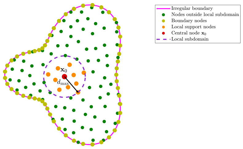
Figure 2.
Comparison of the approximate and exact solutions and the corresponding absolute errors for the real part (a,b) and the imaginary part (c,d) of Example 1 with and .
Figure 2.
Comparison of the approximate and exact solutions and the corresponding absolute errors for the real part (a,b) and the imaginary part (c,d) of Example 1 with and .
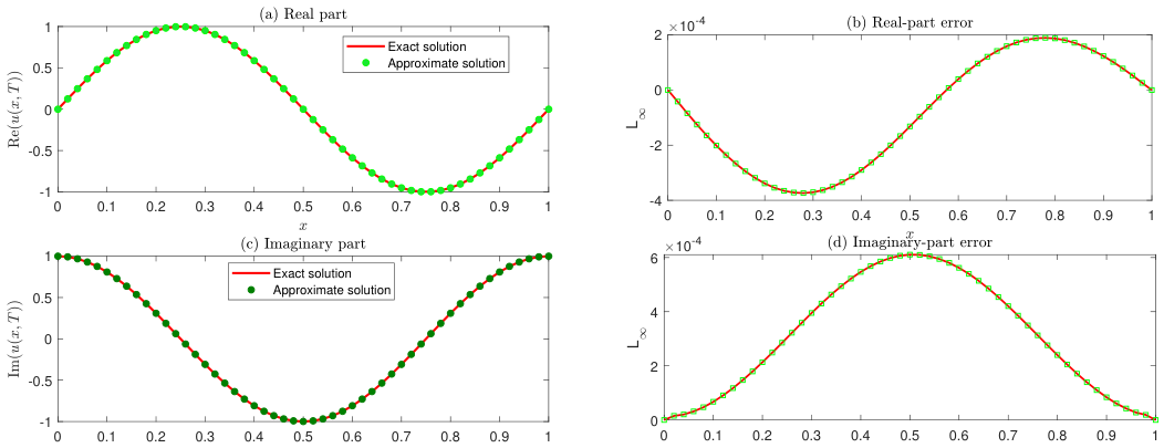
Figure 3.
Comparison of the approximate and exact solutions and the corresponding absolute errors for the real part (a,b) and the imaginary part (c,d) of Example 2 with and when .
Figure 3.
Comparison of the approximate and exact solutions and the corresponding absolute errors for the real part (a,b) and the imaginary part (c,d) of Example 2 with and when .
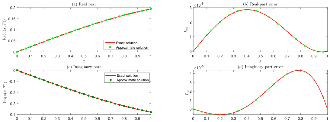
Figure 4.
Numerical real and imaginary parts of the solution, the corresponding absolute error, and the wave density at the final time for Example 3: (a) numerical real part, (b) numerical imaginary part, (c) absolute error, and (d) wave density .
Figure 4.
Numerical real and imaginary parts of the solution, the corresponding absolute error, and the wave density at the final time for Example 3: (a) numerical real part, (b) numerical imaginary part, (c) absolute error, and (d) wave density .
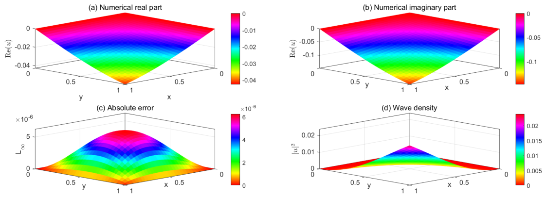
Figure 5.
Numerical and exact solutions, the corresponding absolute error, and the wave density for Example 4: (a) numerical solution, (b) exact solution, (c) absolute error, and (d) wave density .
Figure 5.
Numerical and exact solutions, the corresponding absolute error, and the wave density for Example 4: (a) numerical solution, (b) exact solution, (c) absolute error, and (d) wave density .
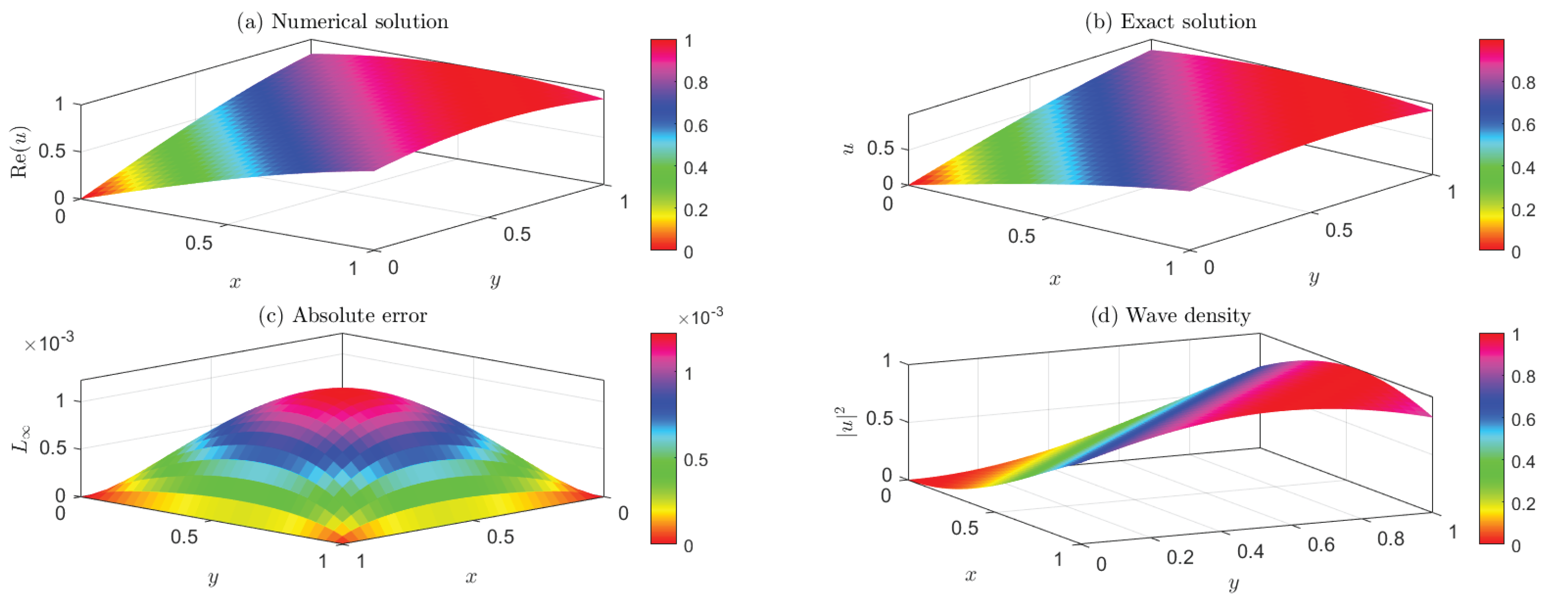
Figure 6.
Numerical and exact solutions, the corresponding absolute error, and the wave density on the irregular domain in Example 4: (a) numerical solution, (b) exact solution, (c) absolute error, and (d) wave density .
Figure 6.
Numerical and exact solutions, the corresponding absolute error, and the wave density on the irregular domain in Example 4: (a) numerical solution, (b) exact solution, (c) absolute error, and (d) wave density .
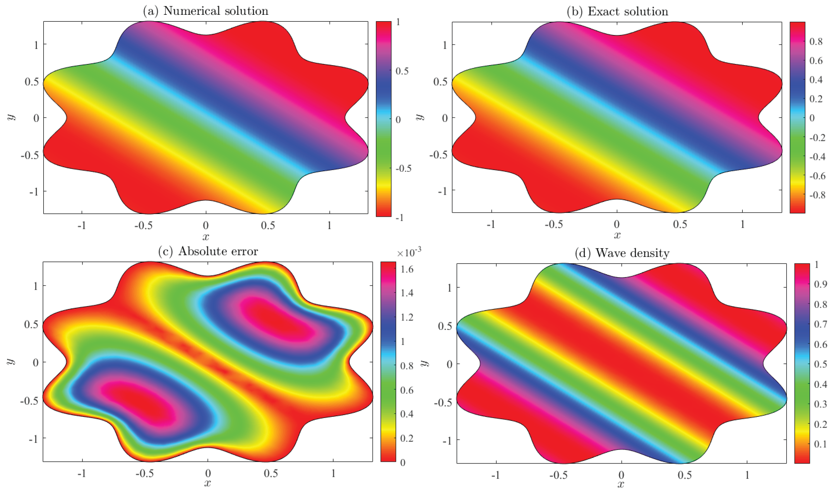
Figure 7.
Numerical solutions and corresponding absolute errors for and in Example 5: (a) numerical solution of , (b) absolute error of , (c) numerical solution of , and (d) absolute error of .
Figure 7.
Numerical solutions and corresponding absolute errors for and in Example 5: (a) numerical solution of , (b) absolute error of , (c) numerical solution of , and (d) absolute error of .
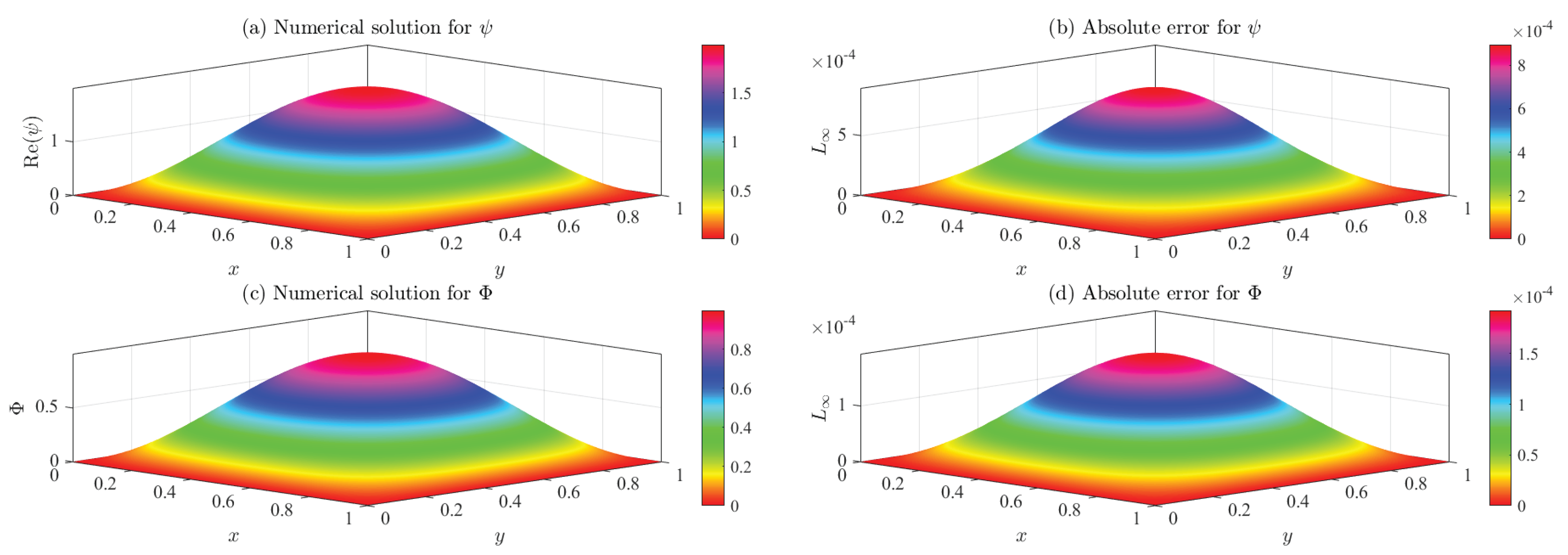
Figure 8.
Numerical solutions and corresponding absolute errors for and on the irregular domain in Example 5: (a) numerical solution of , (b) absolute error of , (c) numerical solution of , and (d) absolute error of .
Figure 8.
Numerical solutions and corresponding absolute errors for and on the irregular domain in Example 5: (a) numerical solution of , (b) absolute error of , (c) numerical solution of , and (d) absolute error of .
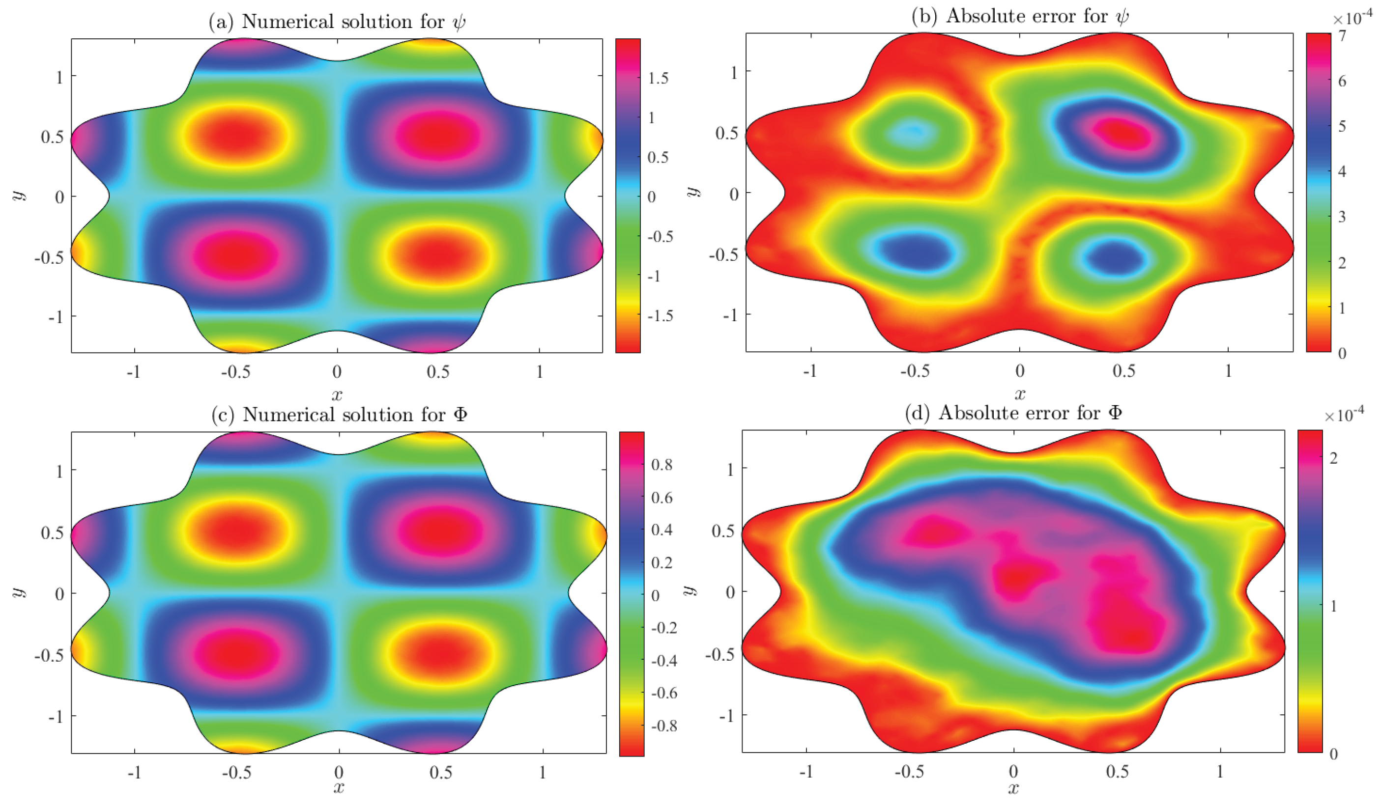

Table 1.
Errors in the real and imaginary parts, errors, and temporal convergence rates for Example 1 at different values of .
Table 1.
Errors in the real and imaginary parts, errors, and temporal convergence rates for Example 1 at different values of .
| Real | Imaginary | Real | Imaginary | |||||
| − | − | |||||||
Table 2.
Real, imaginary, and errors for various spatial discretizations and selected fractional orders in Example 1.
Table 2.
Real, imaginary, and errors for various spatial discretizations and selected fractional orders in Example 1.
| N | ||||||
| Real | Imaginary | Real | Imaginary | |||
| 10 | ||||||
| 15 | ||||||
| 20 | ||||||
| 25 | ||||||
| 30 | ||||||
Table 3.
Numerical errors and CPU times at different final times and fractional orders, with , for Example 1.
Table 3.
Numerical errors and CPU times at different final times and fractional orders, with , for Example 1.
| T | Error measures | CPU (s) | |||||
| Real | Imaginary | RMS | |||||
Table 4.
Errors in the real and imaginary components, error norms, and temporal convergence rates for Example 2 at various values of .
Table 4.
Errors in the real and imaginary components, error norms, and temporal convergence rates for Example 2 at various values of .
| Real | Imaginary | Real | Imaginary | |||||
| − | − | |||||||
Table 5.
Errors in the real and imaginary components, errors, and temporal convergence rates for Example 2 at different values of .
Table 5.
Errors in the real and imaginary components, errors, and temporal convergence rates for Example 2 at different values of .
| Real | Imaginary | Real | Imaginary | |||||
| − | − | |||||||
Table 6.
Numerical errors at distinct final times and fractional orders, with , for Example 2.
| T | Error measures | CPU (s) | |||||
| Real | Imaginary | RMS | |||||
Table 7.
Errors in the real and imaginary components, errors, and temporal convergence rates for Example 3 at different values of .
Table 7.
Errors in the real and imaginary components, errors, and temporal convergence rates for Example 3 at different values of .
| Real | Imaginary | Real | Imaginary | |||||
| − | − | |||||||
Table 8.
Errors in the real and imaginary components, errors, and temporal convergence rates for Example 3 at different values of .
Table 8.
Errors in the real and imaginary components, errors, and temporal convergence rates for Example 3 at different values of .
| Real | Imaginary | Real | Imaginary | |||||
| − | − | |||||||
Table 9.
Numerical errors and CPU times at several final times and fractional orders with for Example 3.
Table 9.
Numerical errors and CPU times at several final times and fractional orders with for Example 3.
| T | Error measures | CPU (s) | |||||
| Real | Imaginary | RMS | |||||
Table 10.
Errors in the real and imaginary components, errors, and temporal convergence rates for Example 4 at different values of .
Table 10.
Errors in the real and imaginary components, errors, and temporal convergence rates for Example 4 at different values of .
| Real | Imaginary | Real | Imaginary | |||||
| − | − | |||||||
Table 11.
Errors in the real and imaginary components, errors, and temporal convergence rates for Example 4 at several values of .
Table 11.
Errors in the real and imaginary components, errors, and temporal convergence rates for Example 4 at several values of .
| Real error | Imaginary | Real error | Imaginary | |||||
| − | − | |||||||
Table 12.
Numerical errors and CPU times at various final times and fractional orders with for Example 4.
Table 12.
Numerical errors and CPU times at various final times and fractional orders with for Example 4.
| T | Error measures | CPU (s) | |||||
| Real | Imaginary | RMS | |||||
Table 13.
Numerical errors and the corresponding convergence rates for and in Example 5 for different values of when .
Table 13.
Numerical errors and the corresponding convergence rates for and in Example 5 for different values of when .
| − | − | − | − | |||||
Table 14.
Numerical errors and the corresponding convergence rates for and in Example 5 for various values of when .
Table 14.
Numerical errors and the corresponding convergence rates for and in Example 5 for various values of when .
| − | − | − | − | |||||
Table 15.
Numerical errors for and at various final times and fractional orders , with , for Example 5.
Table 15.
Numerical errors for and at various final times and fractional orders , with , for Example 5.
| T | |||||||
| RMS | RMS | ||||||
Disclaimer/Publisher’s Note: The statements, opinions and data contained in all publications are solely those of the individual author(s) and contributor(s) and not of MDPI and/or the editor(s). MDPI and/or the editor(s) disclaim responsibility for any injury to people or property resulting from any ideas, methods, instructions or products referred to in the content. |
© 2026 by the authors. Licensee MDPI, Basel, Switzerland. This article is an open access article distributed under the terms and conditions of the Creative Commons Attribution (CC BY) license (http://creativecommons.org/licenses/by/4.0/).
Copyright: This open access article is published under a Creative Commons CC BY 4.0 license, which permit the free download, distribution, and reuse, provided that the author and preprint are cited in any reuse.