

Submitted:
14 September 2026
Posted:
16 September 2026
You are already at the latest version
Abstract
Fast and reliable detection of faults in electric motors is a critical element of properly functioning industrial systems. This paper presents a comprehensive comparative analysis of machine learning algorithms, probabilistic models and deep neural networks in the task of classifying mechanical and electrical faults in DC motors. Two different analytical approaches were proposed and verified in the study. The first, based on the extraction of structured statistical features from longer signal waveforms, was used to evaluate generative models (GNB, QDA), ensemble tree models (Random Forest, XGBoost) and Bayesian Logistic Regression. The second approach, dedicated to real-time systems, consisted of analysing raw 2-millisecond time windows using a two-channel LSTM recurrent network (analysing current and rotational speed signals) and a GNB reference model for flattened sequential data. The results of the experiments confirmed the high effectiveness of both approaches, showing the highest accuracy of XGBoost and QDA models (95%) for tabular data and LSTM networks (93%) for raw time signals. The evaluation and final selection of optimal architectures provide a foundation for further research on the rigorous quantification of epistemic and aleatoric uncertainty in industrial predictive diagnostics.
Keywords:
fault detection
; electric motor diagnostics
; machine learning
; deep neural networks
; Bayesian inference
; uncertainty quantification
; time-series analysis
; statistical features
1. Introduction
Due to increasing industry automation, there is a growing need for electric motors that enable fast and trouble-free operation of production lines [1]. They are an integral part of various types of robots and machines. Their failures, which cause production stops, can lead to huge financial losses [1]. That is why it is so important to quickly detect all types of faults and know their causes. Currently, the most commonly studied method of fault detection is the use of machine learning models, in particular neural networks [2][3]. Some studies compare the accuracy of device classification based on the type of fault detected. However, as other articles show, simply calculating the accuracy of a model does not provide us with relevant information on whether the calculated metric is reliable for the correct detection of faults under real-world conditions [4,5,6]. In particular, in the case of out-of-distribution data, standard metrics can give a false sense of confidence, leading to a “silent” degradation of model performance [6,7].
Experiments are conducted on carefully prepared data, often disregarding problems in model training that may result from a lack of relevant data, measurement noise, or an overly accurate fitting of the pattern [5,8]. The authors of many articles [5,8,9] indicate that the key step is to distinguish and model two types of uncertainty:
The way to take them into account is to create appropriate metrics and quantification methods that allow one to assess the reliability of model decisions and reject uncertain predictions [4,6,7]. This article focuses on analyzing the measurements of an electric motor, processing input data, and selecting and training machine learning models. Based on this work, measurement uncertainties will be modeled according to the methodology described in the literature [4,6]. In the first chapter, we will focus on analyzing the causes of electrical motor damage, methods to measure data indicating motor faults, and methodologies for the preparation of data and the selection of machine learning models. The next stage will describe the measurements used in the research, the method of data processing and division, and the selection, configuration, and training of models.
According to [1], the most common electrical motor faults are classified according to three main components of the machine:
- rolling bearings – responsible for a significant proportion of mechanical failures
- stator – stator damage mainly includes failures of the frame, core, and stator windings. The most common and critical failure in this group is inter-turn short circuit caused by insulation degradation [1].
- rotor – the most common damage is broken rotor cage bars and damage to clamping rings [1].
In many scientific studies, one of the methods used to detect damage is the use of machine learning models trained on the basis of various types of measurements. One of the most commonly used techniques is Motor Current Signature Analysis (MCSA) [10]. This method, based on the analysis of current measurements, allows the detection of mechanical and electrical damage, such as static and dynamic eccentricity, rotor bar cracks, or bearing damage [1,10]. According to many articles, another measurement whose analysis allows the detection and recognition of damage is the measurement of rotor speed [11]. Through fluctuations in rotational speed, we can recognize a mechanically damaged motor (broken rotor bars, damaged bearings) or detect electrical failure (power supply problems, short circuits) [11,12].
Having an appropriate set of measurement data does not necessarily mean having data for model training. Due to the specific nature of time measurements, both for current intensity and rotational speed, the selection of models requires additional data processing. The available literature mentions three basic methods of processing this type of data:
- Spectrograms – an approach based on the transformation of measurement data over time into time-frequency images [13,15]. The signal is divided into time windows, each of which undergoes a Fourier transform – Short Time Fourier Transform (STFT). The resulting spectrograms (a graphical representation of STFT) are treated as images and used to train convolutional neural networks (CNN). The effectiveness of this method in bearing and engine diagnosis has been confirmed, among others, in the work of Verstraete et al. [15], where time-frequency images were used for automatic extraction of damage features.
- Time windows – An approach that involves feeding the raw signal divided into short segments (time windows) into the model without prior transformation to the frequency domain. This method has gained popularity thanks to the development of Deep Learning. As demonstrated by the authors of the article [14], the application of 1D-CNN directly to the raw motor current signal allows high detection efficiency at a lower computational cost and without the need for manual feature selection. Recurrent networks (LSTM) are also often used here [14].
- Statistical features – A classic approach based on the calculation of specific numbers from experiments, such as: mean, root mean square (RMS), kurtosis, shape factor, median, standard deviation, or skewness [16]. The scalars calculated in this way serve as input to the models. The most commonly mentioned here are classic machine learning models (k-Nearest Neighbors, RandomForest, Support Vector Machines, Gaussian Naive Bayes) [2] and probabilistic models such as Bayesian Logistic Regression [6,8], which allow direct estimation of prediction uncertainty.
The main contributions of this work are as follows:
- We demonstrate the effectiveness of various machine learning and deep learning methodologies on a novel, unique dataset of electric motor faults. Because this specific dataset has no direct equivalents in the current literature, our comparative analysis provides a highly valuable and original benchmark.
- We establish a rigorous, highly optimized baseline framework using nested cross-validation. These robust baseline models will serve as a fundamental starting point for future research focused on uncertainty quantification in predictive maintenance, particularly using Bayesian approximations and Monte Carlo Dropout architectures.
2. Materials and Methods
2.1. Data source
Data from the DUDU-BLDC dataset [17] containing measurements from brushless DC motors was used to train the models. The measurements were performed under four operating conditions: efficient, with mechanical imbalance, with deterioration of electrical properties (partial demagnetization of the rotor) and with combined mechanical and electrical faults. Data recording was performed using two synchronized measurement channels:
- Current measurement: performed with an Allegro ACS712-20 Hall sensor.
- Rotational speed measurement: performed with a Lasergage A2108/LSR laser tachometer.
The signals were sampled at a frequency of 50 kHz and divided into time windows of 0.8 s. The raw voltage values read from the sensors were converted into physical quantities according to the characteristics of the measuring equipment using the following formulas:
where and are the voltages measured at the output of the current sensor and tachometer.
For each of the experiments conducted, the authors also calculated 26 characteristics in the time and frequency domains: mean, standard deviation, maximum value, effective value, peak value, skewness, kurtosis, peak factor, spectrum center, spectrum area, and amplitudes at 1×, 2×, and 3× rotational harmonics — for both current (A) and speed (RPM).
The data were saved in files denoting engine failure classes according to the following key:
- healthy – no mechanical or electrical damage
- healthy_zip – mechanical damage
- foulty – electrical damage
- foulty_zip – both electrical and mechanical damage
2.2. Data Preprocessing
Python was used for data processing, model training and optimization, and comparison of results, along with the following libraries: Pandas, Scikit-learn, NumPy, Matplotlib, Optuna, PyMc, Pytensor, and ArviZ.
The research focused on analyzing the performance of the models using two approaches to representing the input data: statistical features and time windows. During the data preparation phase, each dataset was initially divided into disjoint subsets at the experiment level (to prevent data leakage from the same machine cycle).
- The set of statistical features was divided into training and test sets in a 70:30 ratio. Data from 128 randomly selected experiments were included in the training set, while the test set was created from the remaining 56 experiments. Strongly correlated variables were removed to reduce collinearity, which can lead to unstable parameter estimates and interpretation difficulties. The feature correlation threshold was set at 90%, leading to the removal of 8 statistical features from the training and test sets: CURRENT (A) max, CURRENT (A) rms, CURRENT (A) crest_factor, ROTO (RPM) mean, ROTO (RPM) max, ROTO (RPM) rms, CURRENT (A) Frequency Center, ROTO (RPM) Amp @ 3x RPM.
- The data set with time measurements was divided into training, validation, and test sets in a ratio of 70:15:15, maintaining the division into experiments so that data from one experiment could not be included in separate sets.
After division, the data for both variants were standardized using the Z-score method.
where is the mean and is the standard deviation. The standardized time data were divided into time windows of a fixed length of 100 samples, which at a sampling frequency of 50 kHz corresponds to a window length of 2 ms. This resulted in a training set consisting of 102,272 measurements and validation and test sets of 22,372 measurements each.
To definitively verify the effectiveness of all models, nested cross-validation was implemented, requiring the pooling and subsequent dynamic, repeated splitting of all prepared samples.
2.3. Methods: Statistical Features
The input data for models based on statistical features have a very condensed formula due to the large number of features in a small number of experiments. The size of the data sets does not allow the correct training of advanced deep learning models, but the adopted formula provides a good basis for learning classical machine learning algorithms and probabilistic models. The research focused on comparing the performance of three algorithms families: generative models (GNB, QDA), discriminative models based on decision tree ensembles (Random Forest, XGBoost) and Bayesian discriminative models (Bayesian Logistic Regression) [18].
Generative models learn the joint probability model of the data and labels P(X,Y), on the basis of which the probability is calculated using Bayes’ rules. Discriminative models, on the other hand, directly model the conditional (posterior) distribution or the decision function [19].
- 1.
-
In generative models, the distribution of statistical characteristics of measurement data is very similar to the Gaussian distribution, which has been verified through preliminary visualization and analysis of the data set. For this reason, generative models based on normal distributions were selected as a reference point.
- Gaussian Naive Bayes (GNB) is the simplest generative model that allows one to verify whether class separation is possible based on the distribution of statistical features. This algorithm is characterized by a very fast convergence time and a high resistance to overfitting with small data sets. In the process of hyperparameter tuning (using Grid Search), the variance smoothing parameter was optimized by testing 100 values on a logarithmic scale. Variance smoothing allows for the best fit of the model to the shape of the distribution with an appropriate level of measurement noise tolerance.
- Quadratic Discriminant Analysis (QDA) – a model belonging to the Gaussian Discriminant Analysis (GDA) group estimates a full independent covariance matrix for each class. This allows for the creation of unique correlation structures for each class. In order to prevent numerical errors and problems with feature collinearity, the regularization parameter has been optimized to stabilize the inversion of the covariance matrix.
- 2.
-
Discriminative models based on decision trees are the most commonly used machine learning models to work with tabular data. They allow for high prediction accuracy with well-structured and relatively small data sets.
- Random Forest – a model that uses bagging to combine the results of multiple decision trees. This algorithm copes well with non-linearities, which, combined with rich statistical feature representation, allows for precise classification with a small number of samples. Using Bayesian optimization (Optuna environment), the following parameters were tuned: number of decision trees, tree depth, and number of samples. The appropriate selection of parameters prevents overfitting and underfitting.
- XGBoost – a model that uses boosting to sequentially train successive decision trees that correct the errors of their predecessors. It is resistant to unbalanced classes, which allows it to maintain high accuracy even with unequal amounts of input feature data. In addition, it has a built-in regulation mechanism that prevents overfitting and makes it more stable. Due to its high susceptibility to parameterization, the optimization process (Optuna) searched a wide range of variables, including structural parameters, learning rate, sampling stochasticity, and regularization parameters. The selection of appropriate parameters allows for better generalization and makes the model resistant to measurement noise.
- 3.
-
Bayesian discriminant models are probabilistic models based on Bayesian statistics and are one of the most effective ways to check detection accuracy and model uncertainty. The structure of the Bayesian model allows one to learn the probability distribution of data rather than just learning weights, which allows a more accurate look at the impact of statistical features on damage classification.
- Bayesian Multinomial Logistic Regression – thanks to the use of Monte Carlo sampling methods, it allows for direct modeling of epistemic and aleatoric uncertainty. By generating a probability distribution for each class, the algorithm rejects predictions with low certainty, which occurs when the result of the algorithm is a single value. The configuration of this model focused on defining prior distributions and selecting Markov chain sampling (MCMC) parameters. Normal distributions with a mean of zero and a standard deviation of one were adopted as prior distributions for weight matrices and load vectors. This selection of parameters is a direct consequence of the earlier standardization of statistical features, which ensures an appropriate weight scale and prevents overfitting. The No-U-Turn Sampler was used to determine the full posterior distribution. This model, based on logistic regression, had 4 independent Markov chains configured and was trained with 1000 samples per chain. This configuration allowed for full model convergence, which was confirmed by the Gelman-Rubin statistic value of . The high effective sample size values ( > 3000) and the marginal sampling error () indicate that the model parameters were selected correctly.
However, it should be noted that full inference based on MCMC sampling is characterized by extremely high computational complexity, making it run multiple times in nested cross-validation impractical and computationally unjustified [21]. For this reason, in accordance with generally accepted research practice, an analytical approximation in the form of the Maximum A Posteriori (MAP) estimation. As demonstrated in the literature [18,20], from a mathematical point of view, the search for the peak of the posterior probability distribution with a Gaussian prior distribution is analytically equivalent to classical multinomial logistic regression with L2 regularization (where the inverse of the regularization parameter C corresponds directly to the variance of the prior distribution). Full Markov chain sampling (NUTS) was therefore reserved exclusively for training the final model, in order to conduct an in-depth analysis of uncertainty and precisely determine the weight distributions of individual features.
2.4. Methods: Time Windows
The statistical approach is accurate and allows the most important characteristics to be extracted from the measurement data. However, this approach is problematic from the point of view of real-time fault analysis, as it requires more data and additional calculations. Considering real-time fault analysis, the most desirable approach seems to be fault detection based on data obtained from short measurement segments, such as time windows.
The division of the experimental data into time windows resulted in a very large data set. This, in turn, made it possible to extract another subset – validation data. This set is very important from the point of view of training a neural network, as it allows the tuning of its parameters and prevents overfitting. This approach focused on training a neural network model to detect damage and comparing it with the performance of a generative model based on normal distribution.
- 1.
- Long Short-Term Memory – the LSTM recurrent neural network model was selected for the analysis of time series data. This network was designed to process sequential data. Unlike standard recurrent models, it avoids the vanishing gradient problem. This phenomenon involves a drastic decrease in the value of error gradients during backward propagation in time, which prevents the correct learning of weights for long sequences. The LSTM algorithm can capture new relationships in the data without forgetting previous relationships, which are usually minimized in classic RNNs. The implemented model features a dual-channel data input, comprising parallel streams of raw values: current intensity and rotational speed. The hidden layer of the LSTM network was configured for 128 neurons. To avoid overfitting, a layer based on the Monte Carlo Dropout technique was added after the recurrent layer, which randomly deactivates some connections during training and testing, which is crucial for future uncertainty modeling. MC Dropout is a mathematical approximation of Bayesian inference in deep neural networks, and its implementation focuses on the forced deactivation of individual neurons also in the inference phase, which distinguishes it from the standard dropout layer. The probability of neuronal shutdown was set at . The Dropout layer serves to prevent overfitting during model training. The architecture ends with a fully connected dense layer with a Softmax activation function, responsible for generating the final assignment of a sample to one of the damage classes.
- 2.
- Gaussian Naive Beyes - In order to evaluate the performance of a neural network on raw data during uncertainty modeling, it is important to conduct a comparative analysis with another model. For this purpose, a simple generative model, GNB, was implemented. Due to its characteristics, this model does not allow for the implementation of two input data channels. For this reason, the input data was flattened so that each measurement point in the time window could be treated as a separate feature. In this way, instead of two time series with 100 features each, the algorithm receives a single vector consisting of 200 features, i.e., tabular data that it is able to read. This approach deliberately ignores the sequential nature of the signal and the autocorrelation between neighboring samples. Therefore, the model cannot capture temporal dependencies and operates only on the probability distribution of individual features. To ensure a fair comparative environment, the GNB model underwent rigorous nested cross-validation, including grid search optimization of the variance smoothing parameter in the inner loop, using identical standardized data partitions to those of the LSTM network. Additionally, the model does not require a validation set, so it was combined with the test set to train the model on an identical training set that was not combined with the validation set. Unlike models based on statistical features, in this case, no additional hyperparameter optimization was used, using the default estimator settings.
2.5. Ensemble Methods
Models trained on complete data sets are necessary and sufficient for calculating basic metrics of aleatoric uncertainty. This is due to the characteristics of uncertainty that result from measurement noise. However, this approach does not allow for the calculation of epistemic uncertainty, which is related to the lack of sufficient data. This can be implemented for models that combine the results of multiple predictions, i.e. Random Forest, which uses bagging to combine the results of multiple decision trees. Similarly, Bayesian logistic regression generates multiple potential weight vectors, which naturally translate into the probability distribution of the result. The GNB, QDA, and XGboost models only return point estimates of probability, which makes it impossible to directly determine the uncertainty of the model. To overcome this limitation, a team approach inspired by the Deep Ensembles method was used, adapting it to classical machine learning algorithms. To ensure the diversity of component models (necessary for detecting uncertainty), the Bootstrapping technique was used instead of a simple division of the set. It consists of generating M training sets by drawing samples to replace the original data set. As a result, each of the GNB, QDA, or XGBoost models learns from a slightly different representation of the data. The approach and implementation are discussed in more detail in the article (ref).
3. Results
To rigorously verify the effectiveness of the implemented machine learning algorithms, a detailed analysis of their predictive capabilities was conducted. To ensure an objective evaluation and eliminate the risk of optimism bias, a simple data split was avoided in favor of nested cross-validation performed at the level of independent experiments.
Standard metrics were used to evaluate classification quality: accuracy, precision, sensitivity, and F1-score. The results presented in this section are given as the mean and standard deviation (Mean ± SD) of all cross-validation iterations. They serve as a baseline assessment to verify the stability of the optimized architectures prior to their potential extension with uncertainty modeling.
3.1. Results of the Method Based on Statistical Features
The analyzed dataset consisted of 184 independent experiments, representing a fully balanced distribution of decision classes: no damage (46 experiments), mechanical damage (46), electrical damage (46) and electromechanical damage (46). For the extraction of statistical features, the dataset was divided into 128 training experiments and 56 test experiments, based on which 18 uncorrelated signal features were ultimately selected.
3.1.1. Metrics Analysis

Table 1.
Summary of classification results for models based on statistical features.
| Model | Accuracy | Macro Precision | Macro Recall | Macro F1-Score |
|---|---|---|---|---|
| GNB | ||||
| QDA | ||||
| RandomForest | ||||
| XGBoost | ||||
| Bayesian MLR |
When analyzing the average metrics of cross-validation, it can be observed that the ensemble models based on decision trees—Random Forest (90.2% accuracy) and XGBoost (89.7%)—exhibit the highest generalization performance. The very similar results of these two algorithms confirm the high effectiveness of this type of algorithm in classifying structured tabular data.
Probabilistic algorithms, such as QDA and GNB, achieved slightly lower average results (88.6% and 88.0%, respectively). In the case of the QDA model, a higher standard deviation (±3.1%) is also evident, suggesting greater sensitivity to changes in the structure of the training sets of individual folds. The Bayesian MLR model achieved a result of 89.1%, which represents a successful compromise between stable prediction accuracy and the natural ability to directly model uncertainty.
3.1.2. Confusion Matrix
In order to better understand the nature of the errors made by the models, the results were calculated in a confusion matrix.
Figure 1.
Confusion matrices for machine learning models evaluated on statistical features. (a) Confusion matrix for the Gaussian Naive Bayes (GNB) model. (b) Confusion matrix for the Quadratic Discriminant Analysis (QDA) model. (c) Confusion matrix for the Random Forest model. (d) Confusion matrix for the XGBoost model. (e) Confusion matrix for the Bayesian Multinomial Logistic Regression model.
Figure 1.
Confusion matrices for machine learning models evaluated on statistical features. (a) Confusion matrix for the Gaussian Naive Bayes (GNB) model. (b) Confusion matrix for the Quadratic Discriminant Analysis (QDA) model. (c) Confusion matrix for the Random Forest model. (d) Confusion matrix for the XGBoost model. (e) Confusion matrix for the Bayesian Multinomial Logistic Regression model.
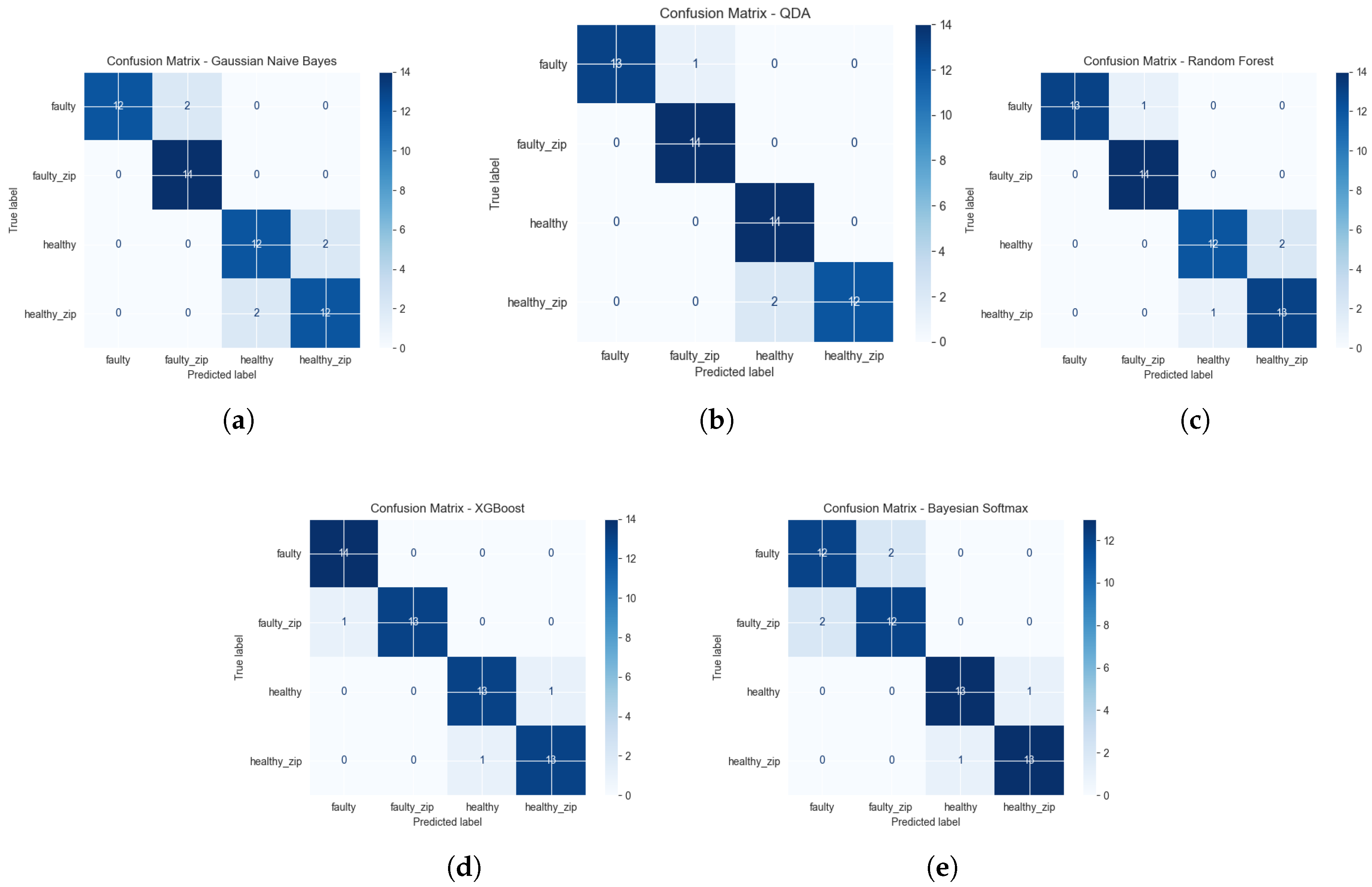
Although summary metrics were used to objectively evaluate the architectures (methodologies) themselves, the final classification models were used for a detailed analysis of errors and the significance of variables. These models, including the full Bayesian variant (MCMC), were trained in the target training set and evaluated in a completely separate test set, maintaining consistency with confusion matrices and weight distributions.
Analysis of the final error matrices demonstrates a very high accuracy of the model in detecting engine failures. None of the models had difficulty distinguishing engines with electrical damage from those without such failures. The main challenge in decision-making was to capture the subtle boundary between mechanically damaged motors and fully functional motors—in this space, the models most frequently made classification errors. The differences between purely electrical faults and electrical-mechanical faults were detected much more reliably and accurately. An interesting exception is the full Bayesian model, which exhibited increased caution in the latter case—it made slightly more errors.
3.1.3. The Impact of Individual Statistical Characteristics on Classification
In order to increase the interpretability of the results, weights were assigned to each feature that influenced the final classification decision for each model. Negative values (indicating a decrease in the accuracy of the algorithm when a given feature is taken into account) were retained in the aggregation process to appropriately penalize parameters introducing information noise. In order to equalize the scales between different architectures, normalization was applied by dividing the raw weight by the sum of the absolute values of all weights in a given model:
Due to this transformation, the total influence of the features adds up to unity (1.0 or 100%), while retaining the original sign (direction) of stimulation. These standardized weights were used to create a global ranking of parameters, determined on the basis of their average influence in all tested architectures.
Table 2.
Feature importance comparison across models.
| Feature | Total | RF | XGBoost | GNB | QDA | Bayesian |
|---|---|---|---|---|---|---|
| CURRENT (A) mean | 14% | 17% | 15% | 27% | 0% | 12% |
| CURRENT (A) std | 13% | 11% | 12% | 17% | 15% | 10% |
| ROTO (RPM) Frequency Center | 10% | 8% | 13% | 12% | 4% | 11% |
| ROTO (RPM) std | 10% | 8% | 12% | 7% | 16% | 6% |
| ROTO (RPM) Spectrum Area | 9% | 7% | 8% | 7% | 14% | 7% |
| CURRENT (A) Spectrum Area | 8% | 9% | 10% | 9% | 2% | 9% |
| CURRENT (A) skew | 6% | 5% | 4% | 4% | 11% | 6% |
| CURRENT (A) kurtosis | 6% | 10% | 8% | -1% | 6% | 5% |
| CURRENT (A) peak_to_peak | 5% | 3% | 3% | 6% | 7% | 4% |
| ROTO (RPM) skew | 4% | 5% | 3% | 3% | 6% | 5% |
| ROTO (RPM) kurtosis | 3% | 4% | 2% | 0% | 4% | 5% |
| CURRENT (A) Amp @ 2x RPM | 2% | 2% | 2% | 0% | 4% | 4% |
| ROTO (RPM) Amp @ 2x RPM | 2% | 2% | 2% | -2% | 2% | 4% |
| CURRENT (A) Amp @ 1x RPM | 2% | 2% | 2% | -2% | 2% | 4% |
| ROTO (RPM) Amp @ 1x RPM | 1% | 1% | 2% | 0% | 4% | 0% |
| CURRENT (A) Amp @ 3x RPM | 1% | 2% | 1% | -2% | 2% | 3% |
| ROTO (RPM) crest_factor | 1% | 2% | 0% | 0% | 1% | 3% |
| ROTO (RPM) peak_to_peak | 1% | 1% | 0% | 0% | 0% | 2% |
The data clearly shows that parameters related to signal power distribution have a key impact on accurate fault detection: mean supply current (CURRENT mean - approximately 14% of overall impact), standard deviation of current (CURRENT std – 13%), the center frequency and standard deviation of rotational speed (ROTO Frequency Center – 10%, ROTO std – 10%), as well as the area under the spectrum (ROTO Spectrum Area – 9%).
However, individual classifiers exhibit different weighting strategies. The Bayesian inference (MLR) model is characterized by the most balanced weight distribution, showing the smallest disparities between individual features, which indicates its high stability and the fact that its predictions are based on a broader diagnostic context. In contrast, the Gaussian Naive Bayes (GNB) model exhibits strong decision polarization—to the greatest extent, up to 27%, it bases its prediction on a single parameter (the average supply current). At the same time, an analysis of negative weights demonstrated that certain parameters, such as kurtosis and the amplitudes of certain rotational speed harmonics (e.g., Amp @ 1x, 2x, 3x RPM), have a marginal or negative impact on the inference process in individual folds, hindering class separation.
3.2. Results of the method based on time windows
For the analysis of rapidly changing signals, the data were divided at the experiment level to generate raw 2-millisecond time windows. The dataset was divided into a training set (128 experiments, resulting in 102,272 sequences), a validation set (28 experiments, 22,372 sequences) and a test set (28 experiments, 22,372 sequences). This rigorous division necessitated the evaluation of models on completely unknown machine operating sequences
3.2.1. Metrics Analysis
Table 3.
Summary of classification results for models based on time windows.
| Model | Accuracy | Macro Precision | Macro Recall | Macro F1-Score |
|---|---|---|---|---|
| GNB | ||||
| LSTM |
Performance metrics calculated for models operating directly on time windows demonstrate the high effectiveness of the deep recurrent LSTM network, which achieved an average accuracy of 95.5% in cross-validation with a relatively low standard deviation (± 1.7%). The result of the probabilistic GNB baseline model (83.2%), which requires operating on an artificially flattened data vector, unequivocally confirms that the time structure and autocorrelation of the signal carry critical diagnostic information. The LSTM network was able to extract this dynamics, increasing the system’s accuracy by more than 12 percentage points.
3.2.2. Confusion Matrix
Figure 2.
Confusion matrices for machine learning models evaluated on time series data. (a) Confusion matrix for the Long-Short Time Memory neural network model. (b) Confusion matrix for the Gaussian Naive Bayes (GNB) model.
Figure 2.
Confusion matrices for machine learning models evaluated on time series data. (a) Confusion matrix for the Long-Short Time Memory neural network model. (b) Confusion matrix for the Gaussian Naive Bayes (GNB) model.
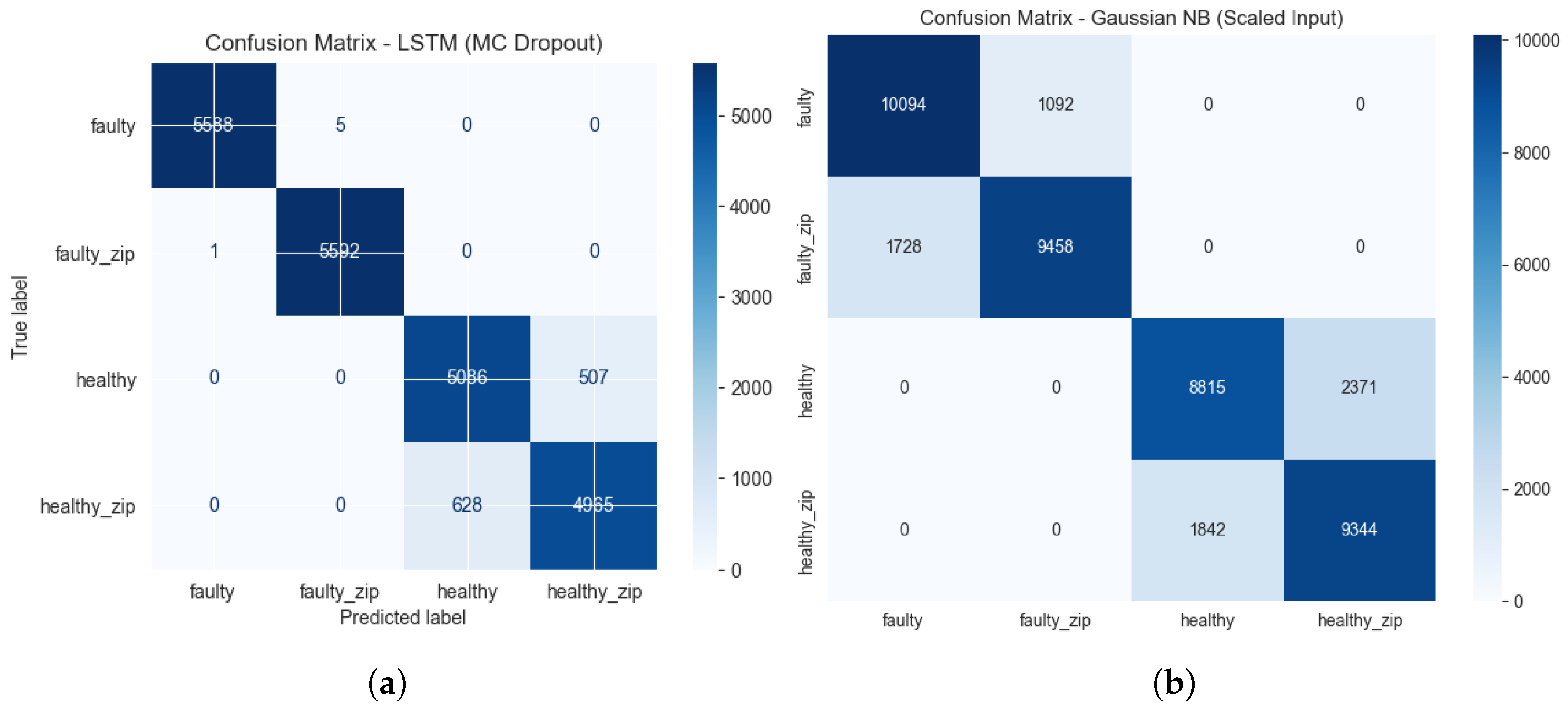
Similarly to models based on statistical features, time-window models are characterized by nearly flawless separation of the electrical failure state from the non-failure state of the machine. Given that the models were tested on datasets comprising more than 22,000 sequences, classification errors between purely electrical faults and electromechanical faults were incidental for the LSTM algorithm. This architecture also demonstrated a significantly lower number of decision errors at the difficult separation boundary between mechanical failures and the absence of damage.
4. Discussion
Algorithms operating on sets of statistical features demonstrate very high accuracy thanks to the strong condensation of diagnostic information in a structured tabular form. This approach allows for the effective learning of discriminative ensemble models based on the structure of decision trees (Random Forest, XGBoost). In turn, empirical feature distributions, showing strong similarity to the normal (Gaussian) distribution, determine the high effectiveness of generative models (GNB, QDA). As shown in the importance analysis of features, classifiers base their decisions to the greatest extent on the standard deviation of the current and rotational speed, the average current value, and the total area under the signal spectrum. Against this background, the model based on Bayesian Logistic Regression stands out with the most balanced distribution of weights, which proves its high decision stability.
On the other hand, algorithms operating directly on raw time windows, although characterized by slightly lower absolute accuracy, have a key advantage, the ability to work in real time. The use of only 2-millisecond signal fragments eliminates the need for time-consuming feature extraction, drastically reducing the system’s response time to a failure. However, the analysis of such short fragments poses a challenge in the form of significant stochastic noise and sudden local current fluctuations. Despite these difficulties, the LSTM deep recurrent network achieved an accuracy of 93%, which is a compromise between the minimum observation time horizon and diagnostic certainty. At the same time, the baseline GNB model proved the usefulness of the probabilistic approach - despite operating on a flattened data vector and losing information about the time structure of the signal, it managed to achieve an effectiveness of 84%.
5. Conclusions
The research conducted has unequivocally confirmed the high effectiveness of classic machine learning algorithms, deep neural networks, and statistical models in the task of detecting DC motor faults. The presented dual methodology proves that the tested architectures can be successfully implemented both for precise, global analysis of historical waveforms (statistical feature-based approach) and for rapid online diagnostics (time window-based approach).
In this paper, classical evaluation metrics (such as accuracy, precision, and confusion matrices) were successfully used to evaluate the models, demonstrating their high predictive performance on a standard test set. The achievement of these results provides a solid foundation, but does not fully address the complex issue of reliable industrial diagnostics.
To verify the safety and stability of the models under real-world, variable operating conditions, it is necessary to examine their robustness against strong measurement noise and limited training data availability. For this reason, as a natural direction for further research, we propose extending the classical evaluation approach with a precise quantification of uncertainty: both aleatory and epistemic. This topic, which is a direct continuation of the present study and builds on the architectures optimized here, is addressed in a separate article [REF].
6. Patents
This section is not mandatory, but may be added if there are patents resulting from the work reported in this manuscript.
Author Contributions
Conceptualization, J.T. and N.S. and W.B.; methodology, J.T. and N.S.; software, J.T.; validation, J.T.; formal analysis, J.T.; data curation, J.T.; writing—original draft preparation, J.T.; writing—review and editing, W.B.; visualization, J.T.; supervision, W.B.. All authors have read and agreed to the published version of the manuscript.
Funding
This research received no external funding.
Data Availability Statement
The source code for the implemented models and the processed datasets is available in the GitHub repository: https://github.com/JakubTom1/Fault-detection-in-mechanical-devices
Conflicts of Interest
The authors declare no conflicts of interest.
Abbreviations
The following abbreviations are used in this manuscript:
| CV | Cross-Validation |
| ESS | Effective Sample Size |
| GDA | Gaussian Discriminant Analysis |
| GNB | Gaussian Naive Bayes |
| LSTM | Long Short-Term Memory |
| MAP | Maximum A Posteriori |
| MC Dropout | Monte Carlo Dropout |
| MCMC | Markov Chain Monte Carlo |
| MCSE | Monte Carlo Standard Error |
| MLR | Multinomial Logistic Regression |
| NUTS | No-U-Turn Sampler |
| QDA | Quadratic Discriminant Analysis |
| RF | Random Forest |
| RNN | Recurrent Neural Network |
| SD | Standard Deviation |
| XGBoost | Extreme Gradient Boosting |
References
- Garcia-Calva, T.; Morinigo-Sotelo, D.; Fernandez-Cavero, V.; Romero-Troncoso, R. Early Detection of Faults in Induction Motors—A Review. Energies 2022, 15. Available online: https://www.mdpi.com/1996-1073/15/21/7855. [CrossRef]
- Esakimuthu Pandarakone, S.; Mizuno, Y.; Nakamura, H. A Comparative Study between Machine Learning Algorithm and Artificial Intelligence Neural Network in Detecting Minor Bearing Fault of Induction Motors. Energies 2019, 12. Available online: https://www.mdpi.com/1996-1073/12/11/2105. [CrossRef]
- Dharmendra, D.; S, S. Motor current signature analysis through machine learning techniques. 2024, 11. [Google Scholar]
- Koblinger, Á.; Fiser, J.; Lengyel, M. Representations of uncertainty: where art thou? In Current Opinion In Behavioral Sciences; 2021; Volume 38, pp. 150–162. Available online: https://www.sciencedirect.com/science/article/pii/S2352154621000577.
- Fakour, F.; Mosleh, A.; Ramezani, R. A Structured Review of Literature on Uncertainty in Machine Learning & Deep Learning. 2024. Available online: https://arxiv.org/abs/2406.00332.
- Lakshminarayanan, B. Introduction to Uncertainty in Deep Learning. Presentation at the CIFAR Deep Learning and Reinforcement Learning (DLRL) Summer School. 2020. Available online: https://www.gatsby.ucl.ac.uk/.
- Incorvaia, G.; Hond, D.; Asgari, H. Uncertainty Quantification of Machine Learning Model Performance via Anomaly-Based Dataset Dissimilarity Measures. Electronics 2024, 13. Available online: https://www.mdpi.com/2079-9292/13/5/939. [CrossRef]
- Weytjens, H.; Verbeke, W. Uncertainty in Machine Learning; 2025; Available online: https://arxiv.org/abs/2510.06007.
- Thuy, A.; Benoit, D. Explainability through uncertainty: Trustworthy decision-making with neural networks. Eur. J. Oper. Res. 2024, 317, 330–340. Available online: https://www.sciencedirect.com/science/article/pii/S0377221723007105. [CrossRef]
- Benbouzid, M. A review of induction motors signature analysis as a medium for faults detection. Ind. Electron. IEEE Trans. On. 2000, 47, 984–993. [Google Scholar] [CrossRef]
- Blödt, M. Condition Monitoring of Mechanical Faults in Variable Speed Induction Motor Drives; Institut National Polytechnique (Toulouse), 2006; Available online: https://ut3-toulouseinp.hal.science/tel-04625555.
- A. Cruz, S.; M. Cardoso, A. Diagnosis of Rotor Faults in Closed-Loop Induction Motor Drives. Conf. Rec. 2006 IEEE Ind. Appl. Conf. Forty-First IAS Annu. Meet. 2006, 5, 2346–2353. [Google Scholar] [CrossRef]
- Valtierra-Rodriguez, M.; Rivera-Guillen, J.; Basurto-Hurtado, J.; De-Santiago-Perez, J.; Granados-Lieberman, D.; Amezquita-Sanchez, J. Convolutional Neural Network and Motor Current Signature Analysis during the Transient State for Detection of Broken Rotor Bars in Induction Motors. Sensors 2020, 20. Available online: https://www.mdpi.com/1424-8220/20/13/3721. [CrossRef] [PubMed]
- Ince, T.; Kiranyaz, S.; Eren, L.; Askar, M.; Gabbouj, M. Real-Time Motor Fault Detection by 1-D Convolutional Neural Networks. IEEE Trans. Ind. Electron. 2016, 63, 7067–7075. [Google Scholar] [CrossRef]
- Verstraete, D.; Ferrada, A.; Droguett, E.; Meruane, V.; Modarres, M. Deep Learning Enabled Fault Diagnosis Using Time-Frequency Image Analysis of Rolling Element Bearings. Shock Vib. 2017, 5067651. Available online: https://onlinelibrary.wiley.com/doi/abs/10.1155/2017/5067651. [CrossRef]
- Tandon, N.; Choudhury, A. A review of vibration and acoustic measurement methods for the detection of defects in rolling element bearings. Tribol. Int. 1999, 32, 469–480. Available online: https://www.sciencedirect.com/science/article/pii/S0301679X9900077. [CrossRef]
- Baranowski, J.; Bauer, W.; Jarzyna, K.; Paweł, P. DUDU-BLDC: Data set for diagnostic of Brushless DC motors with degrading magnets. Zenodo 2025, 5. [Google Scholar] [CrossRef]
- Bishop, C. M. Pattern Recognition and Machine Learning; Springer: New York, 2006; Volume s. 42–44, p. 144-145, 152-153, 196–213, 217-220. [Google Scholar]
- Ng, A.; Jordan, M. On Discriminative vs. Generative Classifiers: A comparison of logistic regression and naive Bayes. Advances In Neural Information Processing Systems, 2001; 14. Available online: https://proceedings.neurips.cc/paper_files/paper/2001/file/7b7a53e239400a13bd6be6c91c4f6c4e-Paper.pdf.
- Murphy, K. P. Machine learning: A probabilistic perspective; MIT Press, 2012; pp. s. 217–220. [Google Scholar]
- Vehtari, A.; Gelman, A.; Gabry, J. Practical Bayesian model evaluation using leave-one-out cross-validation and WAIC. In Statistics and Computing; 2017. [Google Scholar]
Disclaimer/Publisher’s Note: The statements, opinions and data contained in all publications are solely those of the individual author(s) and contributor(s) and not of MDPI and/or the editor(s). MDPI and/or the editor(s) disclaim responsibility for any injury to people or property resulting from any ideas, methods, instructions or products referred to in the content. |
© 2026 by the authors. Licensee MDPI, Basel, Switzerland. This article is an open access article distributed under the terms and conditions of the Creative Commons Attribution (CC BY) license (http://creativecommons.org/licenses/by/4.0/).
Copyright: This open access article is published under a Creative Commons CC BY 4.0 license, which permit the free download, distribution, and reuse, provided that the author and preprint are cited in any reuse.