

Submitted:
15 September 2026
Posted:
16 September 2026
You are already at the latest version
Abstract
Breast histopathology classification is commonly evaluated at the image level even though diagnosis and clinical decisions are made at the patient level. This mismatch can inflate apparent performance when images from the same patient are treated as independent observations and can obscure whether model confidence is reliable across magnifications. We present a reliability-aware framework for patient-level classification on the BreakHis dataset. Four ImageNet-pretrained backbones (ResNet50, EfficientNet-B0, DenseNet121, and Swin-Small) were evaluated using a patient-disjoint split (58/13/11 patients for training/validation/test). ResNet50 and Swin-Small were selected for calibration; temperature scaling was estimated on the validation set, and seven nonlearned aggregation rules combined image probabilities within patients. A compact attention network then learned patient-level weights from calibrated probability, entropy, confidence, magnification, cross-magnification variability, and inter-model disagreement. In an exploratory fixed test set of 11 patients (3 benign, 8 malignant), all four image models produced 0.909 accuracy and 0.833 balanced accuracy after simple patient-level mean aggregation. The learned reliability-aware aggregator reached 1.000 accuracy and balanced accuracy on this small test set as a proof-of-concept result, while its probability-based metrics remained modest (Brier score 0.239; negative log-likelihood 0.671). These findings support the feasibility of reliability-aware patient aggregation but do not establish generalization, because confirmatory patient-aware cross-validation has not yet been completed. The principal contribution is a leakage-conscious evaluation and aggregation workflow, with final comparative claims reserved for the planned cross-validation analysis.
Keywords:
breast histopathology
; BreakHis
; patient-level classification
; calibration
; reliability
; multi-magnification learning
; attention aggregation
1. Introduction
Breast cancer remains one of the most commonly diagnosed cancers among women worldwide, underscoring the clinical value of accurate and efficient diagnostic support tools [1]. Automated analysis of breast histopathology images has the potential to support pathologists by organizing large image collections and identifying patterns associated with malignancy, building on broader advances in applying deep learning to medical image analysis [2]. This potential is reinforced by evidence that diagnostic interpretation of breast biopsy specimens varies substantially among pathologists, with the lowest concordance for borderline categories such as atypia and ductal carcinoma in situ [3]. Deep learning algorithms have already been shown capable of matching or exceeding specialist performance on related tasks, such as detecting lymph node metastases from whole-slide images [4]. A central methodological challenge is that a single patient contributes multiple images, often at several magnification factors made routinely accessible by modern whole-slide scanning systems [5]. Image-level random splits can place images from one patient in both training and evaluation sets, allowing patient-specific appearance to leak across partitions. Moreover, reporting image-level accuracy does not directly represent the patient-level decision that is ultimately of interest.
The BreakHis dataset was introduced to support research on benign and malignant breast tumor classification across 40X, 100X, 200X, and 400X magnifications [6]. Its hierarchical structure motivates two linked questions: how should evidence be combined across images and magnifications for a patient, and how should confidence quality influence that combination? Conventional averaging treats all images as equally informative. Majority voting discards probability magnitude, while confidence weighting may amplify confidently incorrect predictions. A reliability-aware approach should instead use calibrated uncertainty, magnification context, cross-magnification consistency, and model disagreement while preserving patient independence during evaluation.
This study develops and evaluates such a framework. Four convolutional and transformer backbones are trained using patient-disjoint partitions. Temperature scaling calibrates the two selected models [7]. Seven transparent aggregation rules provide interpretable baselines. Finally, a small attention network [8] learns patient-level weights from reliability features without retraining the image backbones. The current manuscript reports the completed fixed-split analysis as an exploratory preprint. The planned patient-aware cross-validation analysis remains necessary before making confirmatory performance claims. Figure 1 illustrates the core contrast between this approach and conventional image-level random splitting.
2. Literature Review
This review covers the four methodological pillars of the present study: deep learning for breast histopathology classification, patient-level evaluation and multiple instance learning, probability calibration, and multi-magnification fusion.
2.1. Deep Learning for Breast Histopathology Image Classification
Deep convolutional neural networks have become the dominant approach for automated classification of breast histopathology images. Residual networks introduced skip connections that enable stable training of very deep architectures [9], compound scaling balances depth, width, and resolution to improve efficiency [10], and densely connected networks reuse feature maps across layers to strengthen gradient flow [11]. Deep learning has also demonstrated strong performance on other histopathology tasks, including skin cancer classification at dermatologist level [12] and mutation prediction from lung cancer histology [13], as well as automated leukemia detection and classification from peripheral blood smear imagery [33]. More recently, the Swin Transformer computes self-attention within shifted local windows, giving it a hierarchical receptive field while retaining the long-range modeling capacity of attention [14]. Systematic comparisons of transformer and convolutional backbones on related gynecologic cytology tasks have found that transformer architectures can match or exceed convolutional baselines once optimization and statistical validation are handled carefully [15,29,30]. The BreakHis dataset has served as a common benchmark for comparing these architectures across the benign-versus-malignant task at four magnifications [6,16]. Bayramoglu et al. proposed a magnification-independent classification approach that learns from images of mixed magnifications, making it an early attempt at multi-magnification generalization on BreakHis [17].
2.2. Patient-Level Evaluation and Multiple Instance Learning
Most published BreakHis results report accuracy at the image level, with little consistent attention to how images from the same patient are partitioned across training and evaluation sets. Subject-level data leakage, where correlated samples from one individual appear on both sides of a split, is a well-documented cause of inflated, non-generalizable performance estimates in medical imaging [18]. This concern applies directly to BreakHis: a single patient contributes dozens of images that share staining, tissue architecture, and acquisition artifacts. A leakage-aware benchmark of leukemia detection confirmed that reported performance can drop substantially once leakage-permissive splits are corrected [19]. Aggregating instance-level predictions into a patient-level decision has been studied extensively under the multiple instance learning (MIL) framework. Campanella et al. demonstrated clinical-grade weakly supervised MIL at scale on whole-slide images [20], and Lu et al. proposed data-efficient MIL for computational pathology [21]. Ilse et al. proposed a learnable attention mechanism that weights instances by their estimated relevance before pooling, outperforming fixed pooling rules on weakly labeled histopathology bags [8]. Beyond imaging, feature selection and dimensionality reduction have similarly been shown to improve classical machine learning models for structured clinical outcome prediction, such as forecasting post-stroke activities of daily living [31]. The present study adopts a patient-disjoint partitioning strategy and extends attention-based pooling to explicitly incorporate calibration and multi-magnification reliability signals.
2.3. Probability Calibration for Deep Networks
Guo et al. showed that modern deep networks tend to be overconfident and that a single learned temperature parameter applied to the logits can substantially reduce calibration error without altering the predicted class [7]. Deep ensembles provide an alternative uncertainty quantification approach with strong empirical performance [22]. Calibration studies on liquid-based cervical cytology have found that ensembles with strong discrimination can still be poorly calibrated, so calibration must be assessed and corrected separately from accuracy-based model selection [23]; the same principle extends to text classification, where reliability-aware calibration and selective prediction have been shown to improve trustworthiness of BERT-based emotion classifiers [24]; a related benchmark of imbalance-handling strategies for fine-grained emotion classification similarly found that a post-hoc temperature-scaling step recovered calibration more dependably than any training-time loss, including focal loss [35]. In oncology outcome prediction, calibration quality has been shown to transfer less consistently than discrimination across cohorts [25], and a decoupled analysis of breast cancer survival prediction across the SEER and METABRIC cohorts found that calibration and explanation reliability can transfer independently of one another under cross-cohort distribution shift [32]. Calibration is especially relevant to patient-level aggregation: rules that combine probabilities across images and magnifications implicitly assume comparable probability meaning, and uncalibrated confidence can distort aggregate decisions even when image-level discrimination is strong.
2.4. Multi-Magnification Fusion and Attention-Based Aggregation
Hashimoto et al. proposed a multi-scale domain-adversarial MIL framework for whole-slide image classification that fuses features across magnifications while remaining robust to noisy instance-level labels [26], illustrating that magnification-aware fusion can outperform single-scale models. Most existing multi-magnification approaches, however, combine features or logits without explicitly modeling how reliable each magnification is for a given patient or incorporating calibrated uncertainty into the fusion weights. A reliability-aware ensemble selection strategy for cervical cytology jointly weighs discrimination, calibration, and selective prediction [27] and pairs calibrated confidence with an uncertainty-aware referral option [28]. A comparable reliability-aware philosophy has been applied outside cytology, converting per-case multimodal CT-MRI registration quality into interpretable Green/Yellow/Red risk categories using data-learned thresholds [34]. The present aggregator shares this philosophy but addresses patient-level combination of multiple images rather than individual-image referral decisions.
3. Materials and Methods
Figure 2 provides an overview of the end-to-end methodology, spanning patient-disjoint dataset design, multi-architecture image-level training and inference, probability calibration and reliability-signal extraction, patient-level aggregation, and statistical evaluation.
3.1. Dataset and Patient-Disjoint Partitioning
BreakHis [6] contains 7,909 microscopy images from 82 patients (24 benign, 58 malignant), including 2,480 benign and 5,429 malignant images acquired at four magnifications. All images belonging to a patient were assigned to a single partition to prevent patient-level data leakage. The split was stratified by class and allocated approximately 70% of patients to training, 15% to validation, and 15% to test. Class labels were assigned at the patient level and inherited by all images from that patient. A random seed of 42 was used for all stochastic operations.

Table 1.
Patient-disjoint dataset partition.
| Partition | Patients | Benign pts. | Malignant pts. | Images |
|---|---|---|---|---|
| Training | 58 | 17 | 41 | 5,242 |
| Validation | 13 | 4 | 9 | 1,504 |
| Test | 11 | 3 | 8 | 1,163 |
| Total | 82 | 24 | 58 | 7,909 |
Figure 3.
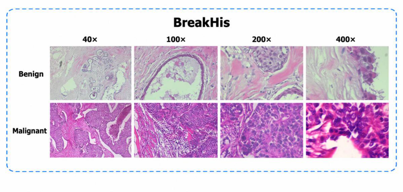
Representative benign and malignant breast histopathology images from the BreakHis dataset at 40×, 100×, 200×, and 400× magnification.
Figure 3.
Representative benign and malignant breast histopathology images from the BreakHis dataset at 40×, 100×, 200×, and 400× magnification.
3.2. Image Classification Models and Training
The image-level stage evaluated ResNet50 [9], EfficientNet-B0 [10], DenseNet121 [11], and Swin-Small [14], all initialized with ImageNet-pretrained weights. For each model, the final classification head was replaced with a single linear layer mapping to one output logit, trained with binary cross-entropy loss (BCEWithLogitsLoss). Training used only the training and validation partitions; the test set was held out entirely.
Training images were preprocessed with random resized cropping to 224 × 224 pixels (scale 0.8–1.0), random horizontal and vertical flips (p = 0.5 each), random rotation up to 15°, and colour jitter (brightness, contrast, and saturation each ±0.10). Evaluation images were resized to 256 pixels and centre-cropped to 224 × 224. All images were normalized to ImageNet channel means [0.485, 0.456, 0.406] and standard deviations [0.229, 0.224, 0.225].
To address the approximately 31/69 benign-to-malignant image imbalance, each sample was assigned a composite weight combining patient-inverse-frequency weighting (to equalize contribution across patients with different image counts) and balanced class weighting. The per-sample loss was computed with BCEWithLogitsLoss(reduction=‘none’) and the composite weight applied before averaging, so no pos_weight argument was used. All models were optimized with Adam (learning rate 1 × 10⁻⁴, weight decay 1 × 10⁻⁴), a batch size of 32, and a maximum of 30 epochs per run. Early stopping used patience of 5 epochs monitored on validation macro-F1. A learning-rate scheduler (ReduceLROnPlateau, factor 0.5, patience 2) reduced the rate when validation macro-F1 plateaued. The random seed was fixed at 42 for all operations.
Swin-Small and ResNet50 were selected as primary and secondary models, respectively, based on their validation-set performance. Swin-Small achieved the highest validation-set macro-F1 and AUROC among the four architectures and was chosen as the primary model for calibration and aggregation. ResNet50 was chosen as the secondary model to provide a CNN-based cross-model disagreement feature. EfficientNet-B0 and DenseNet121 are evaluated at baseline but were not selected for calibration or the learned aggregator.
3.3. Probability Calibration
Because modern neural networks can be poorly calibrated [7], post-hoc temperature scaling was applied to the logits of ResNet50 and Swin-Small using the validation set. The single scalar temperature T was optimized by minimizing validation cross-entropy loss on the logits, without changing predicted class ordering or retraining any weights. Estimated temperatures were T = 1.8426 for Swin-Small and T = 2.6132 for ResNet50; both values greater than 1.0 confirm the expected overconfidence before scaling. EfficientNet-B0 and DenseNet121 were not calibrated; their metrics in Table 2 reflect uncalibrated output probabilities. Calibrated probabilities from Swin-Small and ResNet50 were used in all subsequent reliability features and patient-level aggregation analyses. A limitation of the present fixed-split implementation is that temperature estimation used the complete validation set; nested estimation will be used in the confirmatory cross-validation analysis.
3.4. Nonlearned Patient-Level Aggregation
Seven nonlearned aggregation rules were evaluated for Swin-Small and ResNet50. The rules were: (1) simple mean probability, (2) majority vote, (3) confidence-weighted mean, (4) entropy-weighted mean, (5) equal-magnification mean, (6) magnification reliability-weighted mean, and (7) hierarchical reliability-by-magnification weighting. Equal-magnification averaging computes one probability per available magnification and then averages across magnifications, reducing dominance by magnifications with more images. Magnification reliability weights were estimated from validation patients using leave-one-patient-out calculations for validation reporting; frozen weights from all validation patients were then applied to the test set.
The frozen Swin-Small weights were 0.291, 0.317, 0.100, and 0.100 for 40X, 100X, 200X, and 400X respectively. Corresponding ResNet50 weights were 0.437, 0.469, 0.462, and 0.370. These values should be interpreted as validation-derived relative reliability indicators, not biological importance.
3.5. Learned Reliability-Aware Attention Aggregation
A shared multilayer perceptron mapped each image to an attention score, following the attention-based pooling framework of Ilse et al. [8]. The nine per-image input features were: (1) Swin-Small calibrated malignant probability, (2) Swin-Small calibrated entropy, (3) Swin-Small calibrated confidence, (4–7) a four-dimensional one-hot magnification encoding (40X, 100X, 200X, 400X), (8) patient-level cross-magnification probability standard deviation, and (9) absolute disagreement between Swin-Small and ResNet50 calibrated probabilities for the same image. Scores were normalized within each patient using softmax to produce image-level attention weights that sum to one. The patient-level representation was the attention-weighted sum of the 64-dimensional hidden feature vectors produced by the feature MLP for each image, not a pooled probability. A linear classification head (64→1) then mapped this patient-level vector to an output logit, converted to a malignant probability via sigmoid. Swin-Small calibrated probabilities entered the model only as input feature 1; ResNet50 entered the model exclusively as the disagreement feature (feature 9). Neither backbone’s calibrated probability was used directly as a scored predictor.
The aggregator contained 6,978 trainable parameters: the feature MLP (9→64: 640 parameters; 64→64: 4,160 parameters), the attention branch (64→32: 2,080 parameters; 32→1: 33 parameters), and the classification head (64→1: 65 parameters). Hyperparameters were: hidden width 64, dropout 0.10, Adam optimizer (learning rate 0.001, weight decay 0.0001), maximum 200 epochs, early stopping patience 30, class-balanced BCEWithLogitsLoss. Image backbones remained frozen throughout aggregator training. Training on the 58 training patients stopped after 35 epochs; the best validation checkpoint was at epoch 5.
A known limitation is that the frozen backbones were trained on the same training images used to generate their predictions for aggregator training. The backbone-predicted probabilities for training patients are therefore biased (overconfident), which may inflate training-set aggregator metrics. Although test predictions were generated for unseen patients, the learned aggregator may still be indirectly affected because it was trained using biased in-sample backbone predictions. The confirmatory cross-validation will generate fully out-of-fold backbone predictions to remove this limitation.
3.6. Evaluation
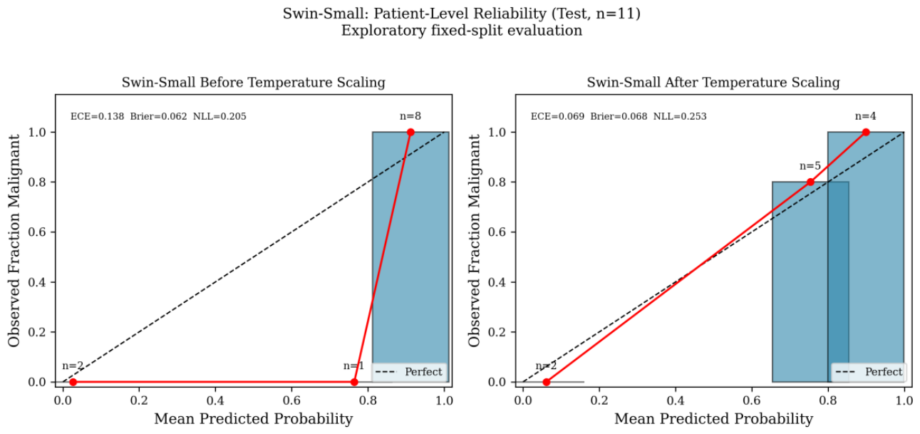
Patient-level discrimination was summarized by accuracy, balanced accuracy, macro-averaged F1, sensitivity, specificity, AUROC, and AUPRC. Probability quality was summarized by Brier score, NLL, and ECE. All patient-level metrics use the mean calibrated probability per patient as the patient-level score for ResNet50 and Swin-Small; for EfficientNet-B0 and DenseNet121, the mean uncalibrated probability is used. ECE values in the reliability diagrams (Figure 6 and Figure 7) are computed at the image level from all test images and therefore differ from patient-level ECE in Table 2; these quantities are not directly comparable. Given only 11 test patients, all estimates have high variance and should be interpreted as descriptive rather than confirmatory.
Figure 4.
Patient-level receiver operating characteristic (left) and precision-recall (right) curves for the four baseline models on the 11-patient test set. DenseNet121 and Swin-Small achieve perfect AUROC. ResNet50 and Swin-Small curves use calibrated probabilities; EfficientNet-B0 and DenseNet121 use uncalibrated probabilities. Exploratory fixed-split evaluation.
Figure 4.
Patient-level receiver operating characteristic (left) and precision-recall (right) curves for the four baseline models on the 11-patient test set. DenseNet121 and Swin-Small achieve perfect AUROC. ResNet50 and Swin-Small curves use calibrated probabilities; EfficientNet-B0 and DenseNet121 use uncalibrated probabilities. Exploratory fixed-split evaluation.
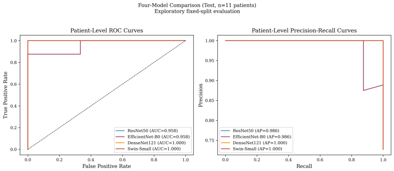
Figure 5.
Patient-level confusion matrices for ResNet50, Swin-Small, and the learned reliability-aware aggregator on the 11-patient test set (3 benign, 8 malignant). The learned aggregator correctly classifies all 11 patients. Exploratory fixed-split evaluation.
Figure 5.
Patient-level confusion matrices for ResNet50, Swin-Small, and the learned reliability-aware aggregator on the 11-patient test set (3 benign, 8 malignant). The learned aggregator correctly classifies all 11 patients. Exploratory fixed-split evaluation.
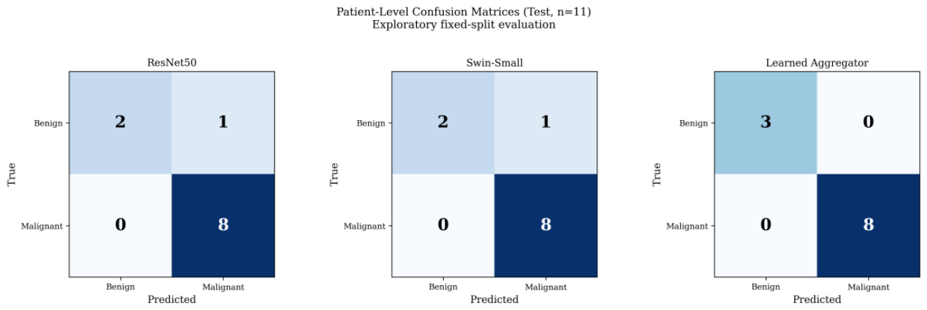
Figure 6.
Image-level reliability diagrams for ResNet50 before (left) and after (right) temperature scaling (T = 2.61, fitted on validation set). Test images, n = 1,163, 5 bins. Image-level ECE = 0.101 before scaling and 0.058 after scaling (notebook Stage 3A output, probECE). These image-level values are not directly comparable to the patient-level ECE = 0.091 reported in Table 2. Temperature scaling reduced both image-level ECE and NLL for ResNet50. Exploratory, not confirmatory calibration evidence.
Figure 6.
Image-level reliability diagrams for ResNet50 before (left) and after (right) temperature scaling (T = 2.61, fitted on validation set). Test images, n = 1,163, 5 bins. Image-level ECE = 0.101 before scaling and 0.058 after scaling (notebook Stage 3A output, probECE). These image-level values are not directly comparable to the patient-level ECE = 0.091 reported in Table 2. Temperature scaling reduced both image-level ECE and NLL for ResNet50. Exploratory, not confirmatory calibration evidence.
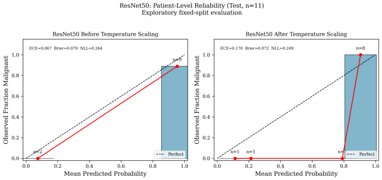
Figure 7.
Image-level reliability diagrams for Swin-Small before (left) and after (right) temperature scaling (T = 1.84, fitted on validation set). Test images, n = 1,163, 5 bins. Image-level ECE = 0.069 before scaling and 0.054 after scaling (as annotated in the figure panels). These image-level values are not directly comparable to the patient-level ECE = 0.138 reported in Table 2. Temperature scaling reduced both Brier score and image-level ECE for Swin-Small. Exploratory, not confirmatory calibration evidence.
Figure 7.
Image-level reliability diagrams for Swin-Small before (left) and after (right) temperature scaling (T = 1.84, fitted on validation set). Test images, n = 1,163, 5 bins. Image-level ECE = 0.069 before scaling and 0.054 after scaling (as annotated in the figure panels). These image-level values are not directly comparable to the patient-level ECE = 0.138 reported in Table 2. Temperature scaling reduced both Brier score and image-level ECE for Swin-Small. Exploratory, not confirmatory calibration evidence.
4. Results
4.1. Baseline Patient-Level Performance
After simple patient-level mean aggregation, all four backbones classified 10 of 11 test patients correctly. All four produced identical accuracy (0.909), balanced accuracy (0.833), and macro-F1 (0.871). DenseNet121 and Swin-Small ranked the 11 patients perfectly by AUROC (1.000) and AUPRC (1.000), but this did not imply correct thresholded classification. DenseNet121 achieved the lowest Brier score (0.055) and NLL (0.167). EfficientNet-B0 achieved the lowest patient-level ECE (0.073). Table 2 reports patient-level ECE for ResNet50 and Swin-Small using their calibrated probabilities, and for EfficientNet-B0 and DenseNet121 using their uncalibrated probabilities, because calibration was not applied to those two models. Differences in probability-based metrics across models should be viewed as descriptive, given the same small test set.
4.2. Nonlearned Patient-Level Aggregation
Table 3 presents the results of all seven nonlearned aggregation rules for Swin-Small and ResNet50 separately. For both models, all seven rules produced identical classification metrics on the test set: accuracy 0.909, balanced accuracy 0.833, and macro-F1 0.871. None of the rules changed a test patient’s predicted class relative to simple mean averaging. Probability scores nevertheless differed across rules. For Swin-Small, equal-magnification mean gave the lowest Brier score (0.067); for ResNet50, hierarchical reliability-by-magnification weighting gave the lowest NLL (0.239). On validation data, one ResNet50 patient changed classification under entropy weighting, reducing validation accuracy to 0.846, illustrating that aggregation rules can affect decisions even when test-set labels remain unchanged. Figure 8 provides a visual comparison of selected representative strategies.
4.3. Learned Attention Aggregation
The learned aggregator matched the best validation classification performance of the transparent rules (macro-F1 0.915, balanced accuracy 0.944) and classified all 11 test patients correctly. However, its Brier score (0.239) and NLL (0.671) indicate that the predicted probabilities remained close to the decision boundary for many patients, so perfect thresholded classification and strong probability quality did not coincide. This should be interpreted as a proof-of-concept result on 11 patients, not as evidence of superiority over the nonlearned rules.
Figure 9.
Patient-level reliability diagram for the learned reliability-aware aggregator. Test set, n = 11 patients, 5 bins. All 11 patients fall into a single bin because predicted probabilities cluster near the decision boundary; the diagram is therefore uninformative for calibration assessment at this sample size. ECE is not reported: with only one populated bin the estimate is not meaningful. Brier score (0.239) and NLL (0.671), reported in Table 4, are the primary probability-quality summaries for this model. Exploratory fixed-split evaluation.
Figure 9.
Patient-level reliability diagram for the learned reliability-aware aggregator. Test set, n = 11 patients, 5 bins. All 11 patients fall into a single bin because predicted probabilities cluster near the decision boundary; the diagram is therefore uninformative for calibration assessment at this sample size. ECE is not reported: with only one populated bin the estimate is not meaningful. Brier score (0.239) and NLL (0.671), reported in Table 4, are the primary probability-quality summaries for this model. Exploratory fixed-split evaluation.
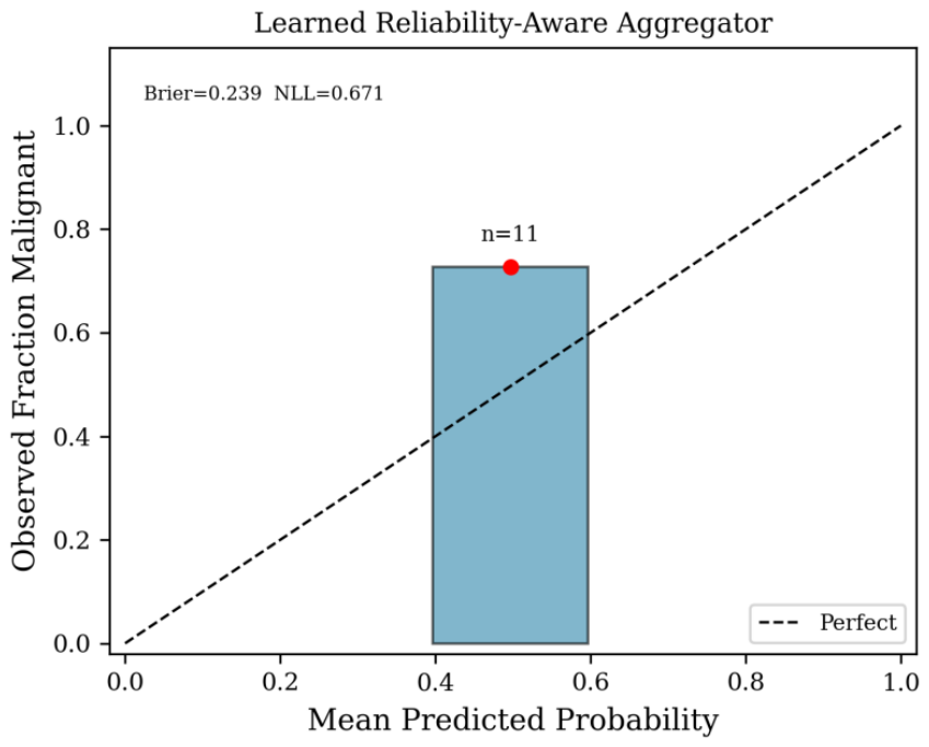
Figure 10.
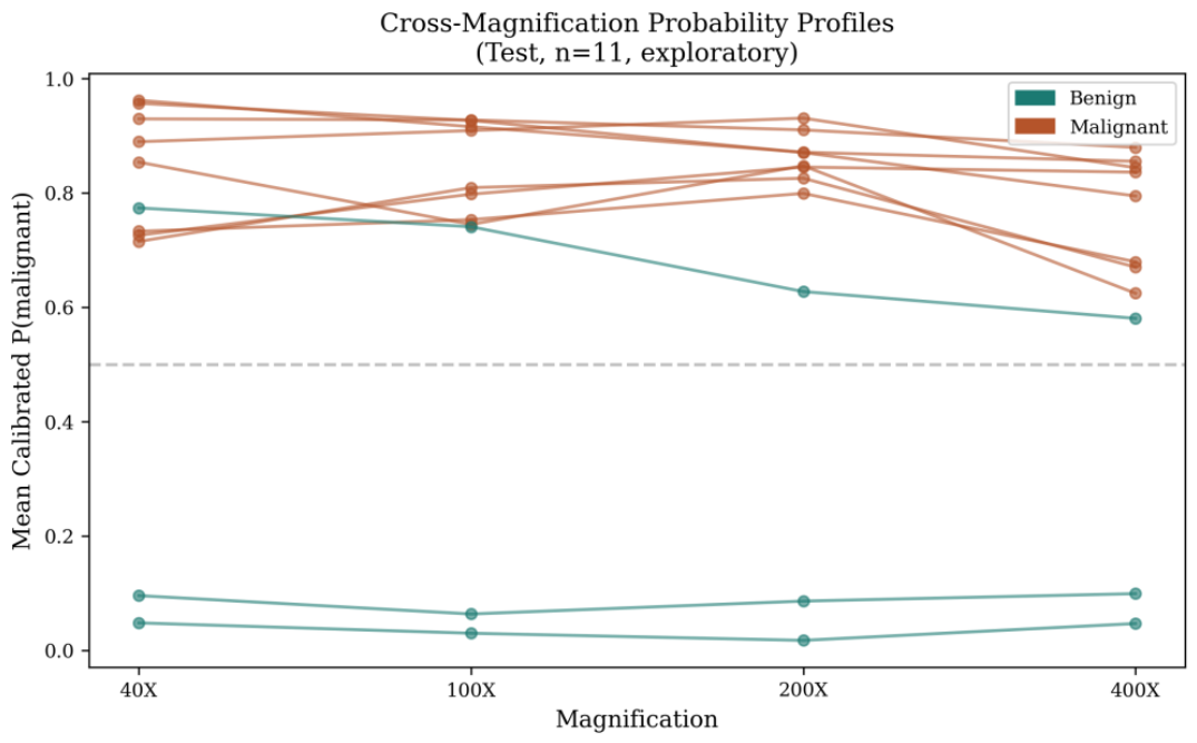
Per-patient cross-magnification probability profiles (Swin-Small, calibrated) on the 11-patient test set. Each line represents one patient. Green lines are benign patients, orange lines are malignant. Exploratory fixed-split evaluation.
Figure 10.
Per-patient cross-magnification probability profiles (Swin-Small, calibrated) on the 11-patient test set. Each line represents one patient. Green lines are benign patients, orange lines are malignant. Exploratory fixed-split evaluation.
5. Discussion
The completed analysis demonstrates that patient-level evaluation provides a different view of image classifiers than image-level reporting. Although DenseNet121 and Swin-Small achieved perfect ranking metrics on the fixed test patients, all four backbones made one thresholded patient-level error under simple averaging. This distinction among ranking, classification, and probability quality is important: no single metric fully characterizes reliability.
Temperature scaling produced mixed calibration results when assessed across multiple metrics. For ResNet50, scaling reduced image-level ECE from 0.101 to 0.058 (n = 1,163 test images, 5-bin estimate; Figure 6), while also reducing Brier score and NLL, consistent with temperature scaling optimizing NLL rather than ECE directly. For Swin-Small, scaling reduced both image-level ECE (from 0.069 to 0.054; Figure 7) and Brier score and NLL, showing more consistent improvement. This mixed pattern reinforces that calibration should be assessed across multiple metrics and confirmed on larger test sets before drawing conclusions.
The nonlearned aggregation rules were stable on the test set. Their failure to change class predictions does not make them redundant: it indicates that the selected test patients were not near enough to the decision boundary for weighting differences to alter labels. The probability-level differences between rules suggest that magnification balancing and reliability weighting can influence confidence, and the observed validation decision change for ResNet50 under entropy weighting reinforces the need to study aggregation rules under repeated patient-level partitions rather than a single fixed split.
The learned attention model produced encouraging proof-of-concept results but should be interpreted cautiously. Perfect classification on 11 test patients is a weak evidence base. The high Brier score and NLL show that accuracy alone overstates confidence quality. The early best epoch (epoch 5 of 200) and small validation cohort create sensitivity to sampling variation. The model’s value is presently methodological: it offers a compact mechanism for combining calibrated uncertainty, magnification context, cross-magnification variability, and model disagreement while keeping the image encoders frozen.
A confirmatory design should generate out-of-fold image predictions for every training patient, fit calibration parameters within each training fold, train the attention aggregator only on out-of-fold predictions, and evaluate on held-out patients. Repeated or stratified group cross-validation should preserve patients as indivisible units. Paired comparisons should operate on identical held-out patients to separate gains due to aggregation from gains due to favorable sampling.
6. Limitations
This study has five principal limitations. First, the test set contains only 11 patients, so all estimates have high variance and perfect scores can arise from a small number of decisions; the results should not be over-interpreted. Second, confirmatory patient-aware cross-validation was not completed; the reported analysis is exploratory. Third, temperature scaling was fitted on the full validation cohort before aggregation analyses; nested estimation inside each cross-validation fold is planned. Fourth, backbone predictions for training patients are biased because the backbones were trained on those images, which may inflate training-set aggregator metrics. Fifth, EfficientNet-B0 and DenseNet121 were not calibrated; their probability metrics reflect uncalibrated outputs and are not directly comparable to calibrated ResNet50 or Swin-Small probabilities.
7. Conclusion
This work introduces a patient-centered, reliability-aware framework for breast histopathology classification across multiple magnifications. The fixed-split results show that calibrated probability aggregation and learned reliability features can be implemented efficiently and produce informative probability-level differences, even when classification labels remain unchanged across aggregation rules. The learned aggregator achieved perfect classification on 11 test patients as a proof-of-concept result; this should not be interpreted as confirmed superiority. Final claims about performance and generalizability will depend on patient-aware cross-validation using fully out-of-fold backbone predictions and appropriately nested calibration.
Author Contributions
Nisreen Albzour: conceptualization, methodology, software, formal analysis, visualization, and writing (original draft).
Funding
This research received no external funding.
Ethics Approval
BreakHis is a publicly available, de-identified research dataset. No institutional review board approval was required for this secondary analysis.
Data Availability
The BreakHis dataset is available from the source described by Spanhol et al. [6], subject to its stated terms of use.
Code Availability
The analysis code is publicly available at https://github.com/Nisreen91/BreakHis-Reliability-Analysis. The BreakHis dataset and trained model checkpoints are not included in the repository.
Competing Interests
The author declares no competing interests.
References
- Sung, H.; Ferlay, J.; Siegel, R.L.; et al. Global cancer statistics 2020: GLOBOCAN estimates of incidence and mortality worldwide for 36 cancers in 185 countries. CA A Cancer J. Clin. 2021, 71(3), 209–249. [Google Scholar] [CrossRef] [PubMed]
- Litjens, G.; Kooi, T.; Bejnordi, B.E.; et al. A survey on deep learning in medical image analysis. Med. Image Anal. 2017, 42, 60–88. [Google Scholar] [CrossRef] [PubMed]
- Elmore, J.G.; Longton, G.M.; Carney, P.A.; et al. Diagnostic concordance among pathologists interpreting breast biopsy specimens. JAMA 2015, 313(11), 1122–1132. [Google Scholar] [CrossRef] [PubMed]
- Ehteshami Bejnordi, B.; Veta, M.; van Diest, P.J.; et al. Diagnostic assessment of deep learning algorithms for detection of lymph node metastases in women with breast cancer. JAMA 2017, 318(22), 2199–2210. [Google Scholar] [CrossRef] [PubMed]
- Pantanowitz, L.; Valenstein, P.N.; Evans, A.J.; et al. Review of the current state of whole slide imaging in pathology. J. Pathol. Inform. 2011, 2, 36. [Google Scholar] [CrossRef] [PubMed]
- Spanhol, F.A.; Oliveira, L.S.; Petitjean, C.; Heutte, L. A dataset for breast cancer histopathological image classification. IEEE Trans. Biomed. Eng. 2016, 63(7), 1455–1462. [Google Scholar] [CrossRef] [PubMed]
- Guo, C.; Pleiss, G.; Sun, Y.; Weinberger, K.Q. On calibration of modern neural networks. Proceedings of the 34th International Conference on Machine Learning (ICML). 2017;70:1321–1330. Available online: http://proceedings.mlr.press/v70/guo17a.html.
- Ilse, M.; Tomczak, J.M.; Welling, M. Attention-based deep multiple instance learning. In Proceedings of the 35th International Conference on Machine Learning (ICML); 2018; 80, pp. 2127–2136. [Google Scholar] [CrossRef]
- He, K.; Zhang, X.; Ren, S.; Sun, J. Deep residual learning for image recognition. In Proceedings of the IEEE Conference on Computer Vision and Pattern Recognition (CVPR), 2016; pp. 770–778. [Google Scholar] [CrossRef]
- Tan, M.; Le, Q.V. EfficientNet: Rethinking model scaling for convolutional neural networks. In Proceedings of the 36th International Conference on Machine Learning (ICML); 2019; 97, pp. 6105–6114. [Google Scholar] [CrossRef]
- Huang, G.; Liu, Z.; van der Maaten, L.; Weinberger, K.Q. Densely connected convolutional networks. In Proceedings of the IEEE Conference on Computer Vision and Pattern Recognition (CVPR), 2017; pp. 4700–4708. [Google Scholar] [CrossRef]
- Esteva, A.; Kuprel, B.; Novoa, R.A.; et al. Dermatologist-level classification of skin cancer with deep neural networks. Nature 2017, 542(7639), 115–118. [Google Scholar] [CrossRef] [PubMed]
- Coudray, N.; Ocampo, P.S.; Sakellaropoulos, T.; et al. Classification and mutation prediction from non-small cell lung cancer histopathology images using deep learning. Nat. Med. 2018, 24(10), 1559–1567. [Google Scholar] [CrossRef] [PubMed]
- Liu, Z.; Lin, Y.; Cao, Y.; et al. Swin Transformer: Hierarchical vision transformer using shifted windows. In Proceedings of the IEEE/CVF International Conference on Computer Vision (ICCV), 2021; pp. 10012–10022. [Google Scholar] [CrossRef]
- Albzour, N.; Lam, S.S. Systematic evaluation of vision transformers for automated cervical cancer classification: Optimization, statistical validation, and clinical interpretability. Cancers 2026, 18(13), 2178. [Google Scholar] [CrossRef] [PubMed]
- Spanhol, F.A.; Oliveira, L.S.; Petitjean, C.; Heutte, L. Breast cancer histopathological image classification using convolutional neural networks. In Proceedings of the International Joint Conference on Neural Networks (IJCNN), 2016; pp. 2560–2567. [Google Scholar] [CrossRef]
- Bayramoglu, N.; Kannala, J.; Heikkilä, J. Deep learning for magnification independent breast cancer histopathology image classification. In Proceedings of the 23rd International Conference on Pattern Recognition (ICPR), 2016; pp. 2440–2445. [Google Scholar] [CrossRef]
- Roberts, M.; Driggs, D.; Thorpe, M.; et al. Common pitfalls and recommendations for using machine learning to detect and prognosticate for COVID-19 using chest radiographs and CT scans. Nat. Mach. Intell. 2021, 3, 199–217. [Google Scholar] [CrossRef]
- Albzour, N. A leakage-aware comparative benchmark of machine learning, deep learning, and transformer models for reliable leukemia detection. arXiv 2026. [Google Scholar] [CrossRef]
- Campanella, G.; Hanna, M.G.; Geneslaw, L.; et al. Clinical-grade computational pathology using weakly supervised deep learning on whole slide images. Nat. Med. 2019, 25(8), 1301–1309. [Google Scholar] [CrossRef] [PubMed]
- Lu, M.Y.; Williamson, D.F.K.; Chen, T.Y.; Chen, R.J.; Barbieri, M.; Mahmood, F. Data-efficient and weakly supervised computational pathology on whole-slide images. Nat. Biomed. Eng. 2021, 5(6), 555–570. [Google Scholar] [CrossRef] [PubMed]
- Lakshminarayanan, B.; Pritzel, A.; Blundell, C. Simple and scalable predictive uncertainty estimation using deep ensembles. Adv. Neural Inf. Process. Syst. (NeurIPS) 2017, 30, 6402–6413. [Google Scholar]
- Albzour, N.; Lam, S.S. Reliability-aware ensemble classification under class imbalance: A calibration study on liquid-based cervical cytology. arXiv 2026. [Google Scholar] [CrossRef]
- Albzour, N. Reliability-aware BERT-based emotion classification via probability calibration and selective prediction. SSRN 2026. [Google Scholar] [CrossRef]
- Albzour, N. External validation and calibration of hybrid deep-boosted ensembles for breast cancer survival prediction: A cross-cohort study on SEER and METABRIC. Research Square 2026. [Google Scholar] [CrossRef] [PubMed]
- Hashimoto, N.; Fukushima, D.; Koga, R.; et al. Multi-scale domain-adversarial multiple-instance CNN for whole slide image classification with imperfect image labels. In Proceedings of the IEEE/CVF Conference on Computer Vision and Pattern Recognition (CVPR), 2020; pp. 3852–3861. [Google Scholar] [CrossRef]
- Albzour, N.; Lam, S.S. Reliability-aware hybrid-K ensemble selection for cervical cytology classification: Integrating discrimination, calibration, and selective prediction. arXiv 2026. [Google Scholar] [CrossRef]
- Albzour, N.; Lam, S.S. Selective prediction and uncertainty-aware referral for pap smear classification. Preprints 2026. [Google Scholar] [CrossRef]
- Albzour, N.; Lam, S.S. Segmentation and classification of pap smear images for cervical cancer detection using deep learning. IISE Annual Conference. Proceedings. Norcross., 2025; pp. 1–6. [Google Scholar] [CrossRef]
- Albzour, N.; Lam, S.S. A reproducible benchmark of ViT-Tiny against CNN baselines for cervical cell classification: accuracy, statistical validation, and deployment efficiency. SSRN 2026. [Google Scholar] [CrossRef]
- Albzour, N.; Agarwal, S.; Althnaibat, H.; Lu, S.S. Predicting post-stroke activities of daily living: enhancing machine learning with feature selection. IISE Annu. Conf. Proceedings. Norcross. 2025, 1–6. [Google Scholar] [CrossRef] [PubMed]
- Albzour, N. Decoupled transferability of calibration and explainability in cross-cohort breast cancer survival prediction. Preprints 2026. [Google Scholar] [CrossRef]
- Al-Zoubi, H.; Al-Bzoor, N. Toward driverless AI: automating leukemia detection and classification using hyperautomation, a case study. Research Square 2022. [Google Scholar] [CrossRef] [PubMed]
- Albzour, N. Reliability-aware CT-MRI registration: a quality engineering framework with stability analysis and risk classification. arXiv 2026. [Google Scholar] [CrossRef]
- Albzour, N. Beyond accuracy: reliability of imbalance-handling strategies for fine-grained emotion classification. SSRN 2026. [Google Scholar] [CrossRef]
Figure 1.
Motivation for patient-disjoint evaluation and reliability-aware aggregation. Top: image-level random splitting allows images from the same patient to appear in both training and test partitions (same-patient leakage), producing discordant per-image predictions and potentially misleading performance estimates. Bottom: the patient-centered approach used in this study keeps all images from one patient together in a single partition, then combines calibrated confidence, uncertainty, inter-model agreement, and magnification context into one patient-level decision aligned with the clinical target.
Figure 1.
Motivation for patient-disjoint evaluation and reliability-aware aggregation. Top: image-level random splitting allows images from the same patient to appear in both training and test partitions (same-patient leakage), producing discordant per-image predictions and potentially misleading performance estimates. Bottom: the patient-centered approach used in this study keeps all images from one patient together in a single partition, then combines calibrated confidence, uncertainty, inter-model agreement, and magnification context into one patient-level decision aligned with the clinical target.
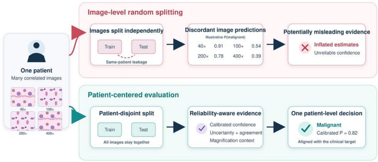
Figure 2.
Overview of the reliability-aware multi-magnification aggregation pipeline, from patient-disjoint dataset design through image-level training and inference, probability calibration, patient-level aggregation (nonlearned rules and learned attention network), and evaluation.
Figure 2.
Overview of the reliability-aware multi-magnification aggregation pipeline, from patient-disjoint dataset design through image-level training and inference, probability calibration, patient-level aggregation (nonlearned rules and learned attention network), and evaluation.
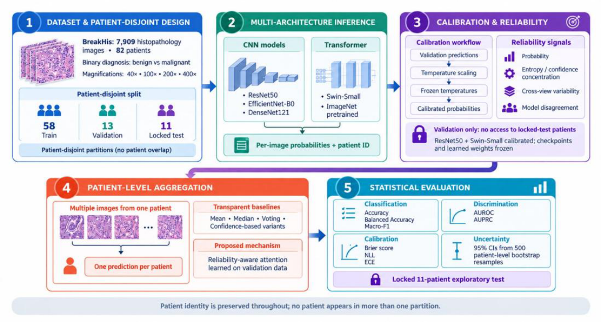
Figure 8.
Visual comparison of five representative aggregation strategies on the 11-patient test set: simple mean, confidence-weighted, entropy-weighted, equal-magnification mean, and full learned aggregator. All four nonlearned strategies produce identical macro-F1 (0.871) and balanced accuracy (0.833); the learned aggregator achieves perfect macro-F1 (1.000) and balanced accuracy (1.000). Remaining nonlearned rules (majority vote, magnification reliability-weighted, hierarchical reliability-weighted) are reported in Table 3; they produce the same classification results as the four nonlearned strategies shown here. Exploratory fixed-split evaluation.
Figure 8.
Visual comparison of five representative aggregation strategies on the 11-patient test set: simple mean, confidence-weighted, entropy-weighted, equal-magnification mean, and full learned aggregator. All four nonlearned strategies produce identical macro-F1 (0.871) and balanced accuracy (0.833); the learned aggregator achieves perfect macro-F1 (1.000) and balanced accuracy (1.000). Remaining nonlearned rules (majority vote, magnification reliability-weighted, hierarchical reliability-weighted) are reported in Table 3; they produce the same classification results as the four nonlearned strategies shown here. Exploratory fixed-split evaluation.
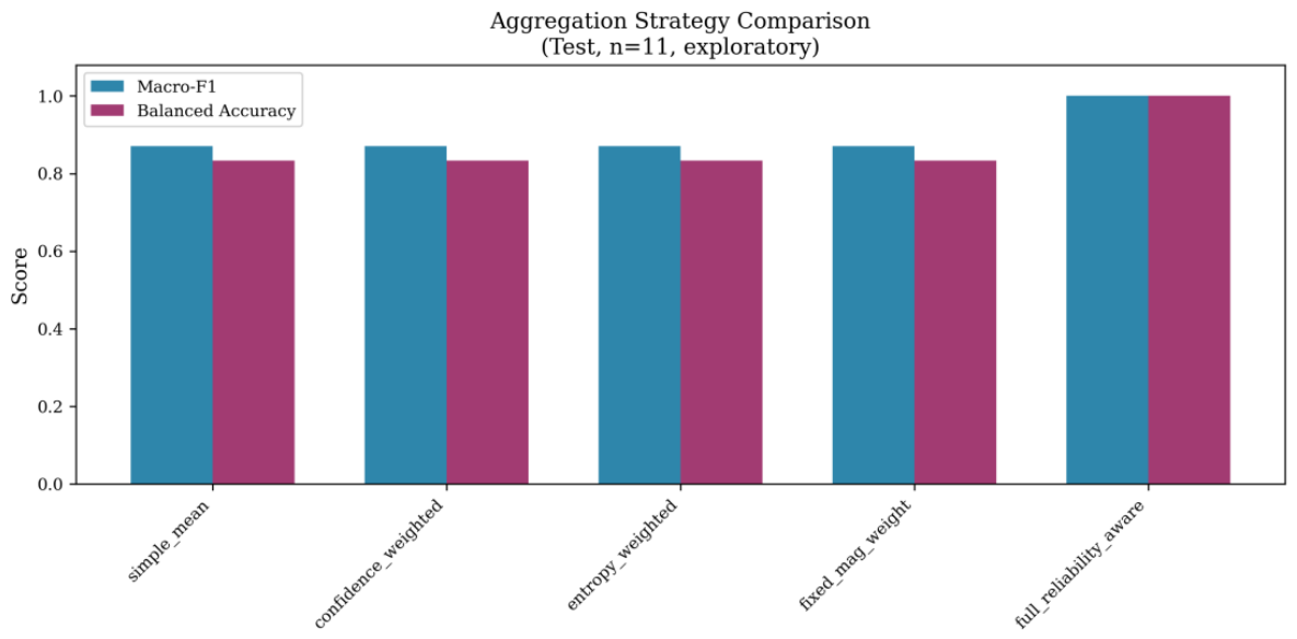
Table 2.
Exploratory fixed-split patient-level performance on 11 test patients. Patient-level score = mean probability per patient, threshold 0.5. ECE uses 15 bins on 11 patients. †Calibrated with temperature scaling (ResNet50 T = 2.61; Swin-Small T = 1.84). *Uncalibrated probabilities (temperature scaling not applied to these models).
Table 2.
Exploratory fixed-split patient-level performance on 11 test patients. Patient-level score = mean probability per patient, threshold 0.5. ECE uses 15 bins on 11 patients. †Calibrated with temperature scaling (ResNet50 T = 2.61; Swin-Small T = 1.84). *Uncalibrated probabilities (temperature scaling not applied to these models).
| Model | Acc. | Bal. acc. | Macro F1 | AUROC | AUPRC | Brier | NLL | ECE |
|---|---|---|---|---|---|---|---|---|
| ResNet50† | .909 | .833 | .871 | .958 | .986 | .079 | .264 | .091 |
| EfficientNet-B0* | .909 | .833 | .871 | .958 | .986 | .072 | .231 | .073 |
| DenseNet121* | .909 | .833 | .871 | 1.000 | 1.000 | .055 | .167 | .107 |
| Swin-Small† | .909 | .833 | .871 | 1.000 | 1.000 | .062 | .205 | .138 |
Table 3.
All seven nonlearned aggregation rules for Swin-Small and ResNet50 on the fixed test set (n = 11 patients). All rules produce identical classification metrics. Probability metrics differ by rule.
Table 3.
All seven nonlearned aggregation rules for Swin-Small and ResNet50 on the fixed test set (n = 11 patients). All rules produce identical classification metrics. Probability metrics differ by rule.
| Model | Aggregation rule | Val. F1 | Val. Bal.Acc. | Test F1 | Test Bal.Acc. | Test Brier | Test NLL |
|---|---|---|---|---|---|---|---|
| Swin-Small | Simple mean | .915 | .944 | .871 | .833 | .068 | .253 |
| Swin-Small | Majority vote | .915 | .944 | .871 | .833 | .072 | .218 |
| Swin-Small | Confidence-weighted mean | .915 | .944 | .871 | .833 | .068 | .249 |
| Swin-Small | Entropy-weighted mean | .915 | .944 | .871 | .833 | .074 | .261 |
| Swin-Small | Equal-magnification mean | .915 | .944 | .871 | .833 | .067 | .251 |
| Swin-Small | Mag. reliability-weighted | .915 | .944 | .871 | .833 | .070 | .256 |
| Swin-Small | Hierarchical rel. weight | .915 | .944 | .871 | .833 | .072 | .253 |
| ResNet50 | Simple mean | .915 | .944 | .871 | .833 | .072 | .249 |
| ResNet50 | Majority vote | .915 | .944 | .871 | .833 | .087 | .340 |
| ResNet50 | Confidence-weighted mean | .915 | .944 | .871 | .833 | .071 | .243 |
| ResNet50 | Entropy-weighted mean | .846† | .844† | .871 | .833 | .076 | .251 |
| ResNet50 | Equal-magnification mean | .915 | .944 | .871 | .833 | .073 | .252 |
| ResNet50 | Mag. reliability-weighted | .915 | .944 | .871 | .833 | .072 | .251 |
| ResNet50 | Hierarchical rel. weight | .915 | .944 | .871 | .833 | .071 | .239 |
†Entropy weighting changed one validation-patient classification for ResNet50, reducing validation accuracy. — Majority vote uses a hard fraction score; Brier/NLL shown for completeness but should be interpreted cautiously for this rule.
Table 4.
Learned reliability-aware attention aggregation results.
| Partition | Patients | Acc. | Bal. acc. | Macro F1 | Sens. | Spec. | AUROC | Brier | NLL |
|---|---|---|---|---|---|---|---|---|---|
| Training† | 58 | .931 | .951 | .922 | — | — | .996 | .235 | .663 |
| Validation | 13 | .923 | .944 | .915 | .889 | 1.000 | .944 | .238 | .670 |
| Test | 11 | 1.000 | 1.000 | 1.000 | 1.000 | 1.000 | 1.000 | .239 | .671 |
†Training metrics are biased because the image backbones were trained on the same images; they are reported only as optimization diagnostics. ECE is not reported for the aggregator: with all 11 test patients in a single probability bin, the ECE estimate is not meaningful.
Disclaimer/Publisher’s Note: The statements, opinions and data contained in all publications are solely those of the individual author(s) and contributor(s) and not of MDPI and/or the editor(s). MDPI and/or the editor(s) disclaim responsibility for any injury to people or property resulting from any ideas, methods, instructions or products referred to in the content. |
© 2026 by the author. Licensee MDPI, Basel, Switzerland. This article is an open access article distributed under the terms and conditions of the Creative Commons Attribution (CC BY) license.
Copyright: This open access article is published under a Creative Commons CC BY 4.0 license, which permit the free download, distribution, and reuse, provided that the author and preprint are cited in any reuse.