

Submitted:
14 September 2026
Posted:
15 September 2026
You are already at the latest version
Abstract
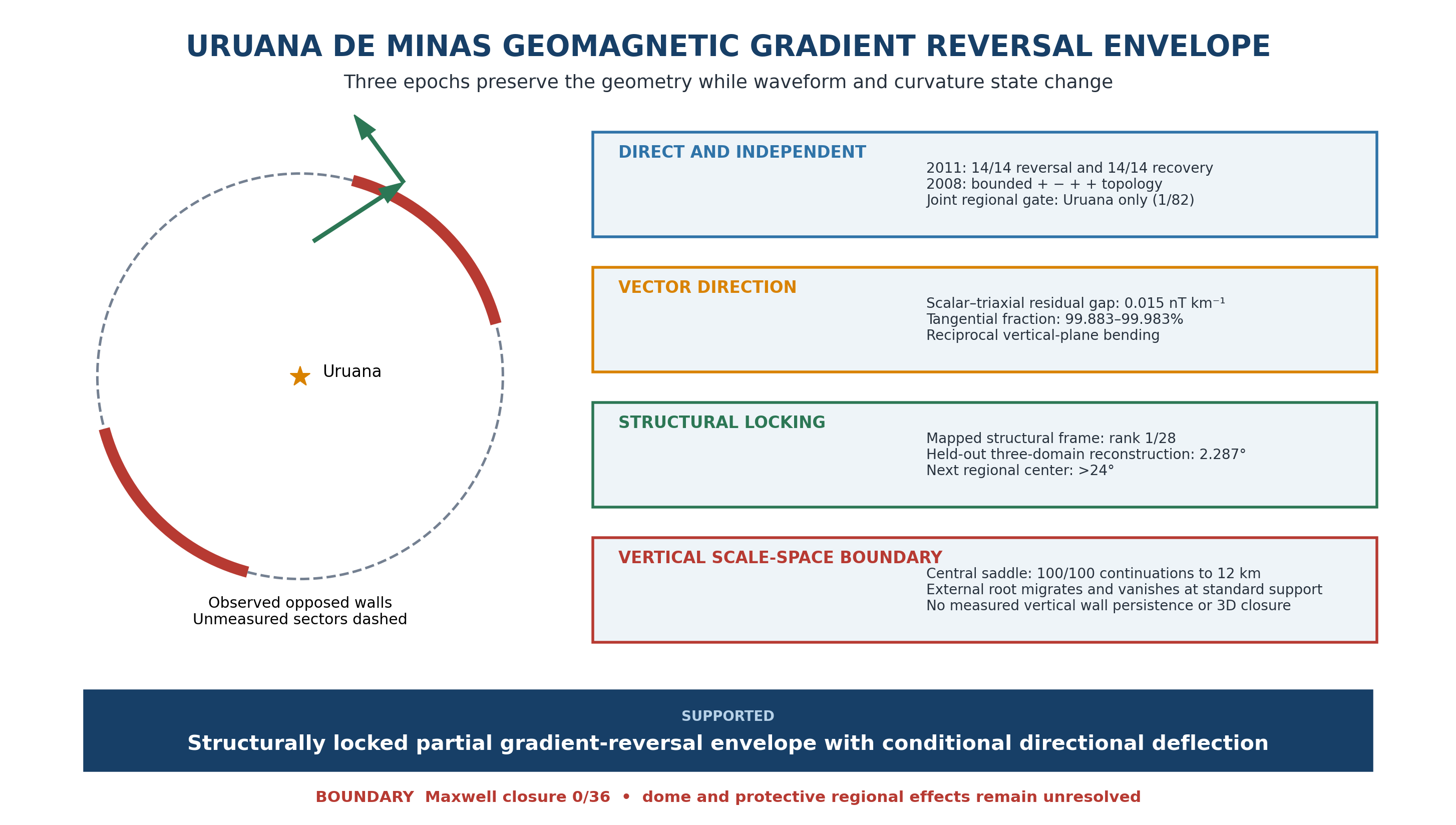
Decades-separated airborne magnetic surveys rarely reproduce amplitude, but a persistent crustal boundary may preserve its geometry. We test this at Uruana de Minas with surveys from 1971–1972, 2008 and 2011. Raw 2011 data show all 14 target lines reverse the positive northward gradient predicted by the International Geomagnetic Reference Field and recover farther north. Independent 2008 data record a bounded positive–negative–positive–positive topology in both scalar data and rotation-invariant triaxial magnitude; together, the two survey gates leave Uruana as the sole joint pass among 82 centers. Historical and 2008 fields recover opposed 7–9 km derivative walls with near-Uruana midpoints, while reciprocal 2008 traverses preserve geographic contrast. Scalar and fluxgate latitudinal residuals differ by 0.015 nT km−1, and the conditional residual direction is 99.883–99.983% tangential. Across 6, 8 and 10 km Hessian supports, six outer curvature roots lie within 0.702 km of the frozen 2011 front, ranking first among 65 translated positions. Under continuation, the outer boundary migrates and disappears by 4 km, whereas the central saddle persists. The surviving frame registers to independently mapped geology. We therefore establish a four-decade, structurally locked magnetic-gradient reversal envelope. Directional deflection remains conditional and Maxwell closure fails; dome closure, circulation and protective effects remain unresolved.
Keywords:
Uruana de Minas
; geomagnetic-gradient anomaly
; airborne magnetometry
; magnetic-gradient envelope
; reciprocal vector deflection
; tangential field change
; meridional-gradient reversal
; antipodal gradient walls
; cross-instrument validation
1. Introduction
Three airborne magnetic surveys crossed the area around Uruana de Minas over four decades, but each preserved the field differently: sparse historical residual profiles in 1971–1972, regional grids and an original scalar–triaxial file in 2008, and raw flight-line observations in 2011. Such archives should not be expected to reproduce scalar amplitude. Survey altitude, line spacing, sampling, acquisition direction, levelling, gridding and filtering determine which wavelengths and derivatives remain visible (Beamish & White, 2011; Gavazzi et al., 2020; Saltus et al., 2026). Edge position and derivative amplitude also vary with observation height, source interference and processing (Lahti & Karinen, 2010; Pilkington & Tschirhart, 2017). The scientific opportunity is therefore more demanding than map-to-map resemblance: which spatial relationships survive when epoch, instrument, support and representation change? Repeated UAV magnetic campaigns show why temporal comparison can separate stable structure from changing state (Guillard et al., 2025; Hokari et al., 2026), while modern inversion work emphasizes explicit control of representation-specific effects such as terrain response (Ito & Utsugi, 2025).
Curvature methods provide a compact way to describe such geometry. For a scalar field F(E,N), a local quadratic approximation defines the horizontal Hessian H, whose eigenvectors are principal-curvature directions and whose eigenvalues carry curvature sign. Curvature and structure-tensor methods are established tools for interpreting potential-field geometry and edges (Phillips et al., 2007; Sertcelik & Kafadar, 2012; Yuan et al., 2014; Yuan & Yu, 2015). Here we use the Hessian for a different inferential question: does a local magnetic eigenframe remain recognizable when survey epoch, spatial support and data representation change, and does that eigenframe correspond to an independently mapped structural grain?
Uruana first appears in the 2011 archive through a simple observation: inside a narrow northern cap, the measured total field falls toward the north although the IGRF rises; farther north, the measured field rises again. That reversal is visible on every usable line before any Hessian or structural comparison is introduced. The older archives then ask whether the same location preserves a recognizable geometry. Project 1009 supplies 1971–1972 historical profiles, Project 0032 supplies a 2008 grid and recovered original file, and Project 3087 supplies the raw 2011 flight lines. We use them in sequence to test whether the sign change belongs to a coherent front, whether independently reconstructed walls occupy opposite sides of a fixed annulus centered near Uruana, whether the organizing frame follows mapped geology, and which three-dimensional source models remain admissible.
Throughout this paper, 'Uruana de Minas geomagnetic-gradient anomaly' denotes the localized, spatially coherent departure of measured scalar total-field gradient geometry from the smooth main-field expectation and same-survey controls. The modifier 'geomagnetic-gradient' names the observed property of Earth's local magnetic field; 'airborne' or 'aeromagnetic' refers only to the acquisition method. 'Antipodal walls' are paired zero crossings of the northward directional derivative dT/dN within the fixed 7–9 km annulus at bearings separated by 180°. 'Structurally locked' means that the negative-curvature eigenaxis remains aligned with the independently mapped structural grain, with its eigenvalue-sign assignment retained across epochs and tested supports, while the independently measured 2011 recovery front lies approximately transverse to that grain; it does not imply fixed magnetization, curvature amplitude, curvature state or three-dimensional envelope geometry. 'Partial annular gradient envelope' denotes the observed opposed sectors, their stable midpoint geometry across epochs and the finite sign-reversal domain. It is an observational term; it does not by itself imply complete 360° or vertical closure, physical shielding, geographic vector reversal or magnetic-polarity reversal.
The study is deliberately mechanism-agnostic. We do not infer a unique source body, mineral, protective effect or geomagnetic polarity reversal. The tested objects are direct line gradients, reciprocal acquisition geometry, rotation-invariant vector magnitude, conditional sensor-frame direction, finite-width turnover topology, nested Hessian phase boundaries, eigenframe orientation, multiscale locking, wrong-fabric substitution, leave-one-domain-out reconstruction and along-fault localization. Regional counts are descriptive robustness screens rather than mutually independent probabilities.
The tests follow a single geographic object through increasingly demanding changes of viewpoint. Raw 2011 lines establish the reversal. The independent 2008 grid tests whether the location survives a different survey and support. Historical and modern derivative walls test bilateral persistence, while Hessian, wrong-fabric and held-out-domain analyses test whether a structural frame survives changes of epoch and scale. Finally, the recovered scalar–triaxial file tests instrument and heading dependence. A closed or dynamic envelope remains a hypothesis motivated by this geometry, not a result assumed by it. Because the evidence paths share data, their convergence is treated as a consistency relation rather than multiplied evidence.
A targeted literature screen therefore asks a narrower novelty question: whether a previously published case combines a kilometre-scale raw scalar-gradient reversal against the smooth main-field expectation with same-line spatial recovery, independent survey generations, stable opposed-wall midpoint geometry across epochs, reciprocal-flight agreement and scalar–triaxial magnitude closure. This conjunction defines documentary primacy in this study; it is not a claim that no other crustal anomaly can contain a local gradient sign change.
2. Geological, Geographic and Survey Setting
Uruana de Minas lies in northwestern Minas Gerais within the broader western São Francisco craton/foreland context adjacent to the Brasília Belt (Pimentel et al., 2011; Alkmim & Martins-Neto, 2012). High-resolution structural information used here comes from the 1:100,000 Projeto Fronteiras de Minas Gerais, Folha Buritis SD.23-Y-D-IV (CODEMIG/UFMG, n.d.). The report describes the sheet as a transition from a more strongly deformed western compartment to a comparatively less deformed central/eastern compartment, with major reverse structures and a pronounced north-south structural grain. Importantly, the structural dataset is not used to define the magnetic target or the 2011 breakpoint chain. The 2022 Census records 3,282 residents in the municipality (IBGE, 2025). At the time of the 1971–1972 survey, Uruana was still a district of Unaí; it was elevated to municipality by State Law 12,030 of 21 December 1995 (Estado de Minas Gerais, 1995). Population and administrative history provide context only and played no role in target definition or candidate selection.
The magnetic datasets are kept separate. Project 1009 (1971-72; SGB, 2026b) supplies historical PGW residual profiles that are predominantly east-west near Uruana. Project 0032 São Francisco (2008; ANP, 2008) supplies 1.5-km regular grids of raw magnetic field (Mag) and a diurnal-corrected representation (mag_var). Project 3087 (2011; SGB, 2026a) supplies raw scalar total-field flight-line measurements from which target slopes, same-line northern controls and free breakpoints are recovered. Table 1 summarizes the role of each dataset.
3. Data and Methods
3.1. Direct 2011 Raw-Field Gate and Free Breakpoints
Raw Project 3087 total-field observations were aggregated into 250-m northing bins to limit along-track pseudoreplication. A flight line was retained when at least five bins (at least 1 km observed support) occurred in the observed +6 to +8 km northern cap of the fixed Uruana target. Fourteen north-south lines satisfy this rule. On each line we fit the raw total field against northing and evaluate IGRF-14 (Beggan et al., 2026) at the 2011 survey epoch and the same spatial support. Thus modeled core-field secular variation is incorporated in the 2011 main-field expectation rather than treated as a fixed modern baseline. The IGRF main-field representation is truncated at spherical-harmonic degree 13, corresponding to spatial wavelengths of order 3,000 km at the equator, so its spatial bandwidth is orders of magnitude coarser than the 8-20 km features analyzed here. Core-field temporal variation can modify the broad background field and gradient, but it does not supply the high-spatial-frequency structure needed to reproduce the localized curvature and turnover geometry; in 2011 this is checked directly because the IGRF gradient remains positive in both zones. The same line is then sampled farther north, using the 16–20 km control band in the principal paired comparison. This design removes between-line zero-level differences because the sign change is evaluated within each individual line.
A strict local signature requires: (i) negative raw target slope, (ii) positive raw same-line northern slope, (iii) positive IGRF slope in both zones, and (iv) a free two-segment breakpoint whose pre/post slopes have negative-to-positive topology. Breakpoint position is optimized before signs are inspected. The 14 frozen breakpoint coordinates are retained unchanged for all later geometric analyses.
For the regional screen, candidate centers are placed on a non-overlapping 16-km lattice and the same strict 2011 logic is applied. The primary full implementation contains 97 centers with at least 14 usable lines. A later reduced reconstruction contains 96 centers but recovers the same six strict centers. The one-center difference arises from the reduced support implementation and does not alter the 82-center common-support cross-survey denominator reported below.
3.2. Independent 2008 Topology and Regional Cross-Survey Gate
For Project 0032, four successive northward intervals are fixed relative to each candidate center: 0–8, 8–16, 16–24 and 24–32 km. Uruana exhibits the sign sequence + - + + in both Mag and mag_var. The regional robustness gate applies five longitude-corridor half-widths (0.75, 1.5, 3, 6 and 9 km) to both channels. A 2008 pass requires the + - + + sequence in all ten realizations. Candidate centers lacking complete 0-32 km 2008 support are not adjudicated by this gate. The strict 2011 and robust 2008 gates are defined separately before intersection.
3.2.1. Recovered 2008 Scalar–Fluxgate and Latitudinal Finite-Difference Audit
The original file 0032_SAO-FRANCISCO_MED_PROC_00237.ASC was recovered from ANP IBM 3592 media. Its identity was verified against archive metadata (133,230,632 bytes; MD5 8022cef7cb949ccb81e0173be9f4fbc5; 1,135,104 data records). It contains simultaneous scalar mag1 and triaxial fluxgate fX, fY and fZ observations. We define the rotation-invariant sensor magnitude Fflux=(fX²+fY²+fZ²)^1/2. The file contains consecutive production lines 10 and 20, flown west-to-east and east-to-west, respectively. Their crossings of the pre-existing São Domingos structural trace were fixed at (-16.0230, -46.1923) and approximately (-15.967942, -46.243126); neither crossing nor the side windows was optimized after inspection of Fflux.
East-minus-west mean steps were calculated in 0.5–3.0 km windows separated by a 1 km exclusion. Robustness crossed nine fixed window pairs (inner 0.5, 1.0, 1.5 or 2.0 km as applicable; outer 2, 3 or 4 km) with two coordinate treatments: records carrying explicit GPS positions (~1 Hz) and sensor-rate records (~10 Hz) whose positions were linearly interpolated only between bracketing GPS epochs. Spatial selectivity used the identical operator at 1 km-spaced centers along line 10 and within ±100 km. Stored fX/fY/fZ remain sensor axes and are never individually renamed as geographic components.
The two reciprocal production lines also form an independent south-to-north finite difference because they are separated by 5.989 km in latitude. Their chord midpoint lies 7.110 km north of the frozen city center, inside the independently defined 2011 +6 to +8 km target cap. At matched meridians, we calculated the cross-line gradient separately for scalar mag1 and the rotation-invariant fluxgate norm. We then decomposed the residual vector derivative relative to the target-excluding regional field into radial magnitude-change and tangential direction-change components at 2, 4 and 8 km support. Five target-excluding reciprocal-axis calibrations and 0.10–1.00 km bin widths test sensitivity. Spatial specificity uses the identical operator at 1 km translations through ±100 km.
Directional analyses remain conditional sensor-frame diagnostics. For the reciprocal torsion test, line 20 is aligned to line 10 by the frozen empirical reciprocal-axis construction, after which inclination and relative-declination steps are evaluated separately on both traverses. A paired three-dimensional reconstruction estimates the background axis only outside ±20 km and tests the perpendicular fraction of the local vector chord. Target-excluding GPS flight-path proxies and IGRF direction provide partial attitude controls. The final closure audit fits sensor-to-body rotation outside the target and asks whether the independently estimated geographic cross-derivatives satisfy dBN/dE=dBE/dN. Missing true roll, pitch and mounting calibration, together with non-coincident finite supports, prevent a definitive geographic magnetic-gradient tensor or field-line reconstruction.
For cross-epoch amplitude localization, the historical +13.750 nT PGW residual step and the 0.5–3.0 km operator were inherited from the prior São Domingos crossing audit. Their agreement with raw mag1 and Fflux was assessed at 1 km translations. These ranks are explicitly post-discovery descriptive controls, not probabilities; the historical points are sparse and the translated windows are autocorrelated.
3.2.2. Three-Flight Finite-Difference Gradient Closure
The two reciprocal east-west production lines and the orthogonal tie-line are treated as three separate flight intercepts, so absolute field levels acquired on different dates are never combined. For each production line, the east-minus-west scalar step is divided by the geographic distance between side-window centroids. Using the observed centroid-displacement unit vector u, the east component is solved from dT/ds = gE uE + gN uN. The archived raw-field slope of tie-line 9120 fixes gN at +2.000811 nT km-1; gE is estimated independently from lines 10 and 20 and then averaged. The sector-scale horizontal axis is theta = atan2(gE,gN). No target angle is fitted.
Sensitivity uses nine fixed side-window definitions (inner limits 0.5-2.0 km; outer limits 2-4 km), leave-one-reciprocal-line reconstructions and a paired translation of the standard 0.5-3.0 km operator through ±100 km. The reconstructed axis is compared with the independently derived 2011 endpoint axis and principal-component-analysis (PCA) turnover-front axis. As a processing-consistency check, an IGRF14 total-intensity gradient is finite-differenced at the 2008 dates and removed from the raw vector; the remainder is compared with the corresponding processed-anomaly reconstruction. This post-discovery test is a sector-scale directional closure, not a pointwise gradient measurement or an independent probability.
3.2.3. Directional-Derivative Zero-Crossing Front
For each 2011 line we define the crustal-overmatch ratio R=−(graw−gIGRF)/gIGRF, where g is the northward scalar total-field gradient. Because gIGRF is positive, R>1 is equivalent to a negative observed gradient. We compare the fixed target and same-line northern-control zones. The line-wise recovery contrast Ci is defined as (graw−gIGRF)control,i−(graw−gIGRF)target,i on the same flight line; its median is a genuinely paired target-control estimator and is kept distinct from the difference between the two zone medians. If the airborne potential field is smooth and a line contains negative and positive directional derivatives in the two zones, the derivative intermediate-value property requires at least one dT/dN=0 crossing between them. This establishes crossing existence, not its pointwise coordinate.
Front orientation is therefore evaluated as an operator envelope rather than from one preferred angle. The exact-site frozen breakpoint coordinates and the uniform regional reconstruction each supply endpoint and PCA axes, giving four 2011 definitions. Every definition is compared with every one of the nine fixed-window 2008 three-flight axes. Leave-one-line-out stability and the six strict 2011 centers are reported descriptively. This audit was developed after discovery and is not assigned an independent probability.
3.2.4. Antipodal 7 to 9 km Envelope Operator
The municipal-seat coordinates of Uruana and the 7–9 km annulus were fixed before the antipodal test. The 7–9 km band was defined as a ±1 km tolerance around the pre-existing 8 km target radius used in the independent 2011 analysis; it was fixed before wall counting and was not selected from the antipodal result. For each 2008 grid representation, dT/dN was sampled on 360 one-degree radial spokes after Gaussian smoothing at 1.5, 3.0 and 4.5 km. A wall was recorded where dT/dN crossed zero within the annulus. Bearings separated by exactly 180 degrees were paired, and we recorded pair count, longest consecutive axial run, opposed-radius mismatch and the midpoint of representative walls. The full horizontal-gradient winding number—the signed net number of complete rotations made by the horizontal-gradient vector along a closed circuit—was measured on concentric circles to distinguish opposed derivative walls from a centered static scalar-field extremum.
Historical Project 1009 PGW is an IGRF-reduced residual product. For each historical realization, an approximate total field was reconstructed by adding the independently evaluated historical IGRF scalar field at the archived survey epoch and altitude before applying the same radial dT/dN=0 wall operator.
Spatial specificity used the identical annulus and antipodal operator at translated centers. All directional bearings in this analysis are azimuths measured clockwise from geographic north; axial differences are evaluated modulo 180 degrees. The separate 2008 audit used 533 centers whose complete 9 km rings lie inside the 2008 grid. The historical audit used 704 centers with complete support in the reconstructed 1971–1972 field. Eighteen historical realizations cross two interpolation methods, three grid spacings and three smoothing scales; six modern realizations cross two scalar channels and three smoothing scales. Their Cartesian product gives 108 historical–modern pairs. Joint comparisons use 407 centers with complete 9 km rings in both grids. For each pair, a translated control survives only when it equals or exceeds both corresponding Uruana counts; Uruana's self-comparison is not evidence. The treatment-wise factorization was identified after inspection of the complete 108-pair sweep and is reported as internal multiverse structure, not as a pre-specified subset or independent test. The eight nonzero-survival centers were subsequently summarized by their minimum circular span and survival-weighted mean azimuth. To separate their concentration from irregular footprint availability, 2,000,000 random eight-center subsets were drawn without replacement from the same 407 eligible centers, and every subset was allowed its own optimal minimum circular sector. This post-discovery reference does not preserve spatial field dependence and is therefore descriptive rather than an anomaly p-value or independent confirmation.
3.3. Historical Line Geometry and 2008 Affine-Row Coherence
Historical Project 1009 coordinates were converted to Universal Transverse Mercator (UTM) zone 23S. Within an 8-km circle, an east-west line is eligible when it contains at least five points, spans at least 4 km east-west and has greater east-west than north-south extent. PGW is regressed against easting independently on each eligible line, and the resulting line slopes are ordered by mean northing. Regional controls use the same 16-km lattice and require at least eight eligible lines. Monotonicity, Kendall ordering and within-line |r| are reported without rescaling the PGW amplitudes.
Two historical-comparability controls were retained. Reconstructed historical total-field slopes were recomputed with both acquisition-era IGRF-1/2 coefficients and retrospective IGRF-14/DGRF. Separately, the 2011 residual field was degraded with a 2 km FWHM low-pass and 2.5 nT quantization to approximate the historical sampling and digitization scale, after which IGRF was restored and line slopes were reevaluated. These tests address IGRF generation and resolution; they do not convert the 1971–1972 residual product into raw flight-line observations.
For the 2008 regular grid, an analogous row-wise operator fits field versus easting on each grid row within 8 km, separately for Mag and mag_var. This tests local affine coherence independently of the later Hessian fit: high row |r| means that the field is nearly linear east-west locally even though the slope of that linear relation may change with northing.
3.4. Local Hessian, Mixed Curvature and Nested Phase Boundaries
Centered local coordinates E and N in kilometres are fit with F(E,N)=a+bE+cN+dE²+eEN+fN². The horizontal Hessian is H=[[2d,e],[e,2f]]. The off-diagonal element e is the mixed partial HEN; eigenvectors provide axial principal-curvature directions and eigenvalues provide curvature sign. Because axes are axial, all orientation differences are reduced modulo 180 deg. For the standard linearized total-field anomaly above its sources, the harmonic potential-field relation gives TEE+TNN+Tzz=0. We therefore recover the scalar vertical second derivative without using any fluxgate axis as Tzz=-tr(H). This derived quantity is vertical curvature of the scalar anomaly, not the geographic magnetic-vector component Bz.
At Uruana, quadratic fits are evaluated over radii 6, 8, 10, 12, 16 and 20 km in both 2008 channels. For nested-phase analysis, sliding Hessians are evaluated along a fixed +2 km east track. Roots of HEN=0 and det(H)=0 are extracted at 6, 8 and 10 km fit radii. For each of the six channel-by-radius outer determinant roots, we additionally calculate the shortest perpendicular distance from its UTM coordinate on that track to the PCA line fitted to the 14 frozen 2011 breakpoints. Neither the 2011 line nor the 2008 roots is refitted for this cross-epoch registration. To supply a spatial denominator, maximum absolute separation was fixed as the primary score before the translated-control ranks were inspected; mean absolute separation was secondary and mean signed position descriptive. Holding PCA orientation fixed, the 2011 line was translated along its normal from −8 to +8 km in 0.25 km steps, giving 65 parallel positions, and the six distances were recomputed at each position. These deterministic competition ranks are not p-values and test perpendicular placement conditional on the frozen orientation, not rotational specificity. The same Hessian operator is translated to regional centers where complete support exists. These roots are post-discovery geometric descriptors; their role is to test reproducibility and relational ordering, not to assign a source depth.
3.5. Tri-Epoch Eigenframe and Multiscale Bridge
The historical positive-curvature axis is obtained from the 1971 local Hessian, and the 2008 positive-curvature axes from the raw and corrected 8-km Hessians. The exact site-level 2011 front is described in two ways: the endpoint direction of the 14 frozen breakpoints and the first PCA axis of the breakpoint cloud. Regional ranking uses a separate uniform reduced reconstruction applied identically across 25 centers with complete 1971, 2008 and 2011 support. This distinction prevents the exact site front from being conflated with the regionalized operator.
Two closely related 1971 Hessian implementations are retained for distinct analyses. The tri-epoch bridge implementation yields a positive-curvature axis of 54.3446 deg (negative axis 144.3446 deg), whereas the structural-frame diagonalization implementation yields a negative-curvature axis of 144.0872 deg. Their axial difference is 0.2574 deg and does not affect any reported rank or interpretation.
To test scale bridging, the 2008 Hessian radius is varied over 6, 8, 10, 12, 16 and 20 km. For each center, one 2008 scale is allowed to minimize mismatch to the historical 1971 axis and independently another scale may minimize mismatch to the 2011 front. The bridge score is the worse of those two best mismatches. Endpoint and PCA front definitions are evaluated separately, and a worst-of-two robust score is also retained.
3.6. Structural Fabric and Bidirectional Scale Locking
The local structural grain is estimated from the Buritis GIS using mapped S-surface traces and contractional/reverse faults, without lithologic contacts. Line segments are weighted by length and summarized by an axial circular mean. The principal analysis uses a 20-km radius; the axial mean-resultant-length statistic R_ax measures directional organization. Two scale stresses are then run mechanically: (i) geology fixed at 20 km while the magnetic Hessian radius varies 6–20 km; and (ii) the 8-km magnetic Hessian fixed while structural buffers vary 10, 15, 20, 25 and 30 km.
The 2011 front is also compared with the structural grain. If one Hessian eigenaxis follows the structural fabric, the orthogonal eigenaxis should lie near a transverse turnover-front family. Exact-site and regionalized front descriptions are reported separately.
For reproducible reuse of the local frame, we additionally freeze a coordinate-referenced angular inventory without assigning inferential weight to rounded values. The primary structural inclination A is the acute angle between geographic north and the independently mapped axial structural grain. The primary transverse direction B is the axial circular mean of two independently fixed bearings: the Uruana-center-to-São-Domingos entry direction, spatialized by the original 2008 line-10 crossing, and the exact 2011 PCA breakpoint-front direction. The line-10 crossing is a proxy approximately 86 m from the mapped exposure-transition endpoint. We also report B−A and B+A as algebraically dependent frame descriptors; they are not additional observations or independent confirmations.
3.6.1. Along-Fault Localization and Label-Withheld Mineral Endpoint
The pre-existing São Domingos audit applies identical side-window steps at successive 2008 flight-line crossings and measures their distance along the mapped contractional trace from its exposed–concealed junction. An orthogonal tie-line acquired 63 days earlier supplies a directional replication near the junction. These tests localize magnetic response along a mapped structure; they do not assume that the cartographic exposure transition is a tectonic bifurcation.
As a secondary independent endpoint, 64 mineral-resource occurrences in the public Buritis inventory were ranked after commodity labels were withheld. The score combined six magnetic and structural realizations; lower rank indicates repeated proximity to high magnetic response and the contractional network. Commodity identity was revealed only for interpretation of the resulting rank. Because the geological compilation may have used geophysical context and the ranking was developed retrospectively, this endpoint is spatial corroboration rather than a blind mineral-discovery test.
3.7. Structural-Frame Diagonalization
To test whether the structural grain acts as a natural coordinate frame for magnetic curvature, H is rotated from geographic E,N coordinates into U,V coordinates with U parallel to the mapped structural axis and V perpendicular. We quantify the off-diagonal fraction q=|HUV|/||H||F and the collapse C=1-qUV/qEN. A value C near one indicates that most apparent mixed curvature in E,N disappears after rotation into the structural frame. The test is applied to both 2008 channels, the 2008 scale ladder and the 1971 historical Hessian. Because the structural frame comes from an independent mapping product, this is not an algebraic eigenvector rotation chosen to diagonalize H.
3.8. Empirical Wrong-Fabric Substitution Test and Cross-Domain Leave-One-Out Reconstruction
Two stringent orientation controls are applied after the primary structural-locking analysis. First, the fixed 8-km 2008 raw and corrected negative-curvature eigenaxes at each of the 28 geology-overlap centers are compared not only with their own mapped structural axis but with all 28 empirical structural axes from the same regional set. No continuous rotation is optimized. The own-fabric rank therefore asks whether the local mapped structure matches its local Hessian better than structurally plausible but geographically wrong alternatives.
Second, three independent orientation domains are placed on the same axial 0-180 deg space: the 1971 negative-curvature Hessian axis, the mean 2008 negative-curvature axis from raw and corrected grids, and the mapped geological structural axis. In leave-one-domain-out reconstruction, two domains reconstruct the third by their axial circular mean; the endpoint is the largest of the three held-out errors. This uses 28 common-support centers and fits no free consensus angle to all three simultaneously.
A four-domain extension adds the normal to the 2011 turnover front, because the front itself is approximately transverse to the negative-curvature/structural family. Endpoint and PCA front descriptions are evaluated separately, each converted to an axial normal by adding 90 deg modulo 180 deg. Each of the four domains is then hidden in turn and reconstructed from the other three by axial circular mean. The conservative four-domain endpoint is the worse of the endpoint- and PCA-based leave-one-out errors. Nine centers have complete support for all four domains.
3.9. Signed Structural Frame, State Changes and Vertical Scale-Space
Axis alignment alone discards the sign assignment of the Hessian eigenvalues. We therefore define a signed structural frame: the mapped structural axis must coincide with the negative-curvature eigen-direction and the orthogonal axis with the positive-curvature direction, with det(H)<0. The historical 1971 Hessian and all 12 2008 radius-by-channel realizations (radii 6, 8, 10, 12, 16 and 20 km; raw Mag and diurnal-corrected mag_var) are evaluated under this same sign convention. Regional comparison uses the worst structural-axis mismatch across epochs and modern realizations.
To separate persistence of the reference frame from persistence of the local curvature state, we also compare Uruana with the immediately adjacent center 16 km west. The test asks whether curvature along a nearly unchanged mapped fabric can change sign without a corresponding rotation of that fabric. Adjacent 16-km center pairs with channel-consensus curvature signs provide the regional control set.
Vertical scale-space is evaluated at two distinct levels. First, the central Hessian is followed through the existing 0–12 km upward-continuation ladder, comprising two channels, two detrending choices and 25 levels. Second, the external det(H)=0 root family is seeded from its native-scale identity on the fixed +2 km east track and followed until branch fusion or loss. This second audit uses 0–12 km continuation, three boundary treatments, supports from 4 to 12 km and a frozen continuity rule. Parallel translated versions of the 2011 PCA front provide a spatial null. The central-saddle and external-boundary endpoints are kept separate because persistence of det(H)<0 at Uruana does not imply persistence of the surrounding det(H)=0 root.
3.10. Regional Controls, Dependency Discipline and Negative Tests
Regional ranks are descriptive robustness controls. Denominators differ among operators because of survey support and eligibility, and ranks are not multiplied. The principal negative controls remain visible: failure of the historical reconstruction to reproduce the 2011-style window-averaged total-field inversion, a centered stationary saddle, topographic tensor alignment, gravity replication, closed scalar contours, the retired 43° hypothesis, reciprocal line order, vertical stationarity of the external root and geographic Maxwell closure. The claims matrix preserves the status and dependency boundary of every promoted result.
As an external operator-control separate from the Uruana anomaly, a metadata-ranked pair of public Alaska aeromagnetic surveys was evaluated under a protocol frozen before confirmatory values were inspected. South National Petroleum Reserve 1977 and Howard Pass 2008 were selected from the declared inventory; the unsigned Hessian-eigenframe hypothesis, 20 km support, pair-selection rule, 899-rotation reference and pass thresholds were fixed prospectively (Gibson & Tailleur, 1980; Brown, 2009; Connard et al., 1999; Johnson et al., 2019). This control tests whether geographic eigenframe registration is recoverable across heterogeneous surveys, not whether the Uruana anomaly transfers to Alaska. The full protocol, genealogy and machine-readable results are retained in Supplementary Files S1 and S2.
3.11. Reproducibility and Computational Assistance
All primary measurements are public third-party data. Supplementary File S2 contains the frozen 2011 breakpoints, complete regional-control tables, structural-frame and leave-one-domain-out tables, the new vector-file audit and deterministic verification scripts. The earlier multiepoch audit is permanently archived at https://doi.org/10.5281/zenodo.22064055; the newly recovered upstream file is identified by filename, byte size and MD5 but is not redistributed.
OpenAI ChatGPT (accessed August–September 2026) was used only as an assistive tool for language editing, code drafting and debugging, and audit organization. The authors conceived the study, defined the methods and inferential rules, selected and verified the data, reviewed all code and outputs, independently confirmed the reported values, interpreted the results and approved the final manuscript. The authors retain full responsibility for the work. No generative-AI images were used.
3.12. Literature screen for Documentary Analogues
A targeted scoping search was completed on 10 September 2026 in Crossref, OpenAlex and publicly indexed web literature. Query families combined aeromagnetic or airborne; total field or scalar; horizontal or meridional gradient; sign reversal or negative gradient; localized or crustal anomaly; IGRF or main field; reciprocal flight lines; repeated or multiepoch survey; scalar-vector or fluxgate corroboration; and remanent magnetization. Candidate records were screened from titles, abstracts and full text where available. A close documentary analogue had to report a spatially localized raw scalar total-field gradient opposite to the smooth main-field expectation and an independent validation by same-line recovery, a separate survey generation, reciprocal acquisition or scalar-vector agreement. The screen did not systematically cover non-English, proprietary, unindexed, unpublished or technical-report literature; documentary primacy is therefore restricted to the explicitly searched and publicly accessible corpus. This was a bounded novelty screen, not a systematic census of every magnetic dataset worldwide.
3.13. Anthropogenic-Confounder Screen
We screened mapped human infrastructure around the frozen center (16.0593° S, 46.2585° W) without changing the pre-existing spatial design. The 8 km target disk remained primary; a 16 km disk was used only as a sensitivity envelope. Built-up and rural land-cover fractions were calculated from the 10 m ESA WorldCover 2021 v200 product (Zanaga et al., 2022). Major energy infrastructure was queried from ANEEL transmission-line and substation services and the SIGA generation register (ANEEL, 2026a,b). Active mineral-process polygons were intersected from ANM SIGMINE with legal phase retained, because a process polygon does not establish an operating mine (ANM, 2026). OpenStreetMap/Overpass supplied a supplementary inventory of settlements, major roads, towers, aerodromes and tagged industrial, quarry and power features (OpenStreetMap contributors, 2026).
Distances were calculated from the frozen center. The primary inferential test was joint scale and chronology: whether any mapped installation had the size, geometry and age needed to explain a coherent kilometre-scale response recurring across survey generations. Present-day layers were not treated as reconstructions of 1971. Absence from volunteered geographic information was considered corroborative only; official ANEEL and ANM records supplied the principal infrastructure tests. Small local objects, distribution wiring and unmapped features were not assumed absent.
4. Results
The evidence is presented in the order in which the anomaly becomes progressively harder to dismiss: a raw 2011 sign reversal, an independent 2008 topology, a bilateral geometry that persists across decades, a frame tied to mapped structure, and finally the directional and physical-closure tests. Each stage addresses a different failure mode. Its control set remains separate from the others, and the resulting ranks are never multiplied.
4.1. The 2011 Raw Measurements Independently Establish the Local Gradient Reversal
The first result requires no derived geometry. All 14 usable 2011 target lines have negative raw northward slopes, with a median of −1.555 nT km−1, although the corresponding IGRF gradients are positive (median +0.993 nT km−1). Farther north, the same 14 lines return to positive raw slopes (median +0.963 nT km−1), while IGRF remains positive (median +1.023 nT km−1). Every line changes in the same direction from target to control; the median raw change is +2.578 nT km−1 and the minimum is +0.549 nT km−1.
The lines comprise seven northbound and seven southbound traverses acquired on 27, 28 and 30 May 2011. The target-negative/north-positive topology persists in the principal supplied magnetic-stage channels and across four shifted 250 m bin phases; one phase gives 13/14 rather than 14/14 only for MAGBRU/MAGCOR, while every northern control remains positive. GPS altitude, barometric altitude, terrain clearance and the digital terrain model do not reproduce the universal magnetic sign pattern.
Free two-segment fitting recovers a negative-to-positive breakpoint on all 14 lines. The frozen breakpoint chain has an exact endpoint axis of 61.776 deg and PCA axis of 63.688 deg. These coordinates are the site-level geometric anchor for later comparisons; they are not moved after geological inspection. Figure 1 shows the paired raw slopes and the frozen front geometry.
The reversal is a relative statement between two gradients evaluated on the same flight-line support: the measured raw meridional gradient and the IGRF main-field gradient. Across the 14 flight lines, the median line-wise residual (raw−IGRF) is −2.607 nT km−1 at the target and +0.267 nT km−1 along the same lines 16–20 km north; their zone-median separation is 2.874 nT km−1. More directly, every within-line control-minus-target residual contrast is positive (14/14), ranging from 0.368 to 7.396 nT km−1 with median 2.922 nT km−1. Thus recovery is not produced by a few influential lines. The anomaly reverses the sign of the total-field gradient on all 14 usable lines, in both flight directions and across three acquisition days, while the raw northern gradients remain positive. Only 6/97 regional centers reproduce the complete strict same-line signature. This scalar total-field gradient reversal is the independent raw-data anchor that fixes Uruana before the multiepoch geometry is examined; it is not evidence of a vector-field or magnetic-polarity reversal.
4.2. Independent 2008 Topology Makes the Cross-Survey Combination Regionally Selective
The independent 2008 grid cannot be compared point for point with the narrower 2011 cap. Its values are regression slopes over four non-overlapping 8 km intervals, whereas the 2011 target statistic is fitted line by line within the +6 to +8 km cap. The positive 2008 0–8 km slope therefore does not contradict the negative 2011 target slope. What the older survey contributes is a separate bounded topology: the raw interval gradients are +0.842, −1.632, +2.217 and +3.113 nT km−1, and the corrected values are +0.810, −1.679, +2.136 and +2.771 nT km−1. Both channels thus recover the same + − + + sequence across all five fixed corridor widths.
The 2011 signature alone is not unique regionally: six of 97 primary candidate centers satisfy the strict 14/14 target-negative/north-positive/IGRF-positive/free-breakpoint gate. Among 82 centers with complete 2008 support, four satisfy the robust 2008 + - + + gate. Their intersection contains one center only: Uruana (1/82). A fully machine-readable reduced reconstruction in Supplementary File S2 contains 96 2011 centers, recovers the same six strict centers, the same 82 with 2008 support, the same four robust 2008 passes and the same unique joint pass. The 1/82 value is a descriptive regional rank, not a probability of worldwide uniqueness.
4.3. Opposed Walls Place Uruana Near a Persistent 8 km Midpoint
The unique cross-survey pass identifies the location; the annulus operator asks what spatial form survives there. In 2008, both Mag and mag_var recover north–northeast and south–southwest dT/dN zero-crossing walls within the fixed 7–9 km annulus at all three smoothing scales. Representative north-wall radii are 7.60–8.49 km and south-wall radii 7.55–8.74 km, with a median radius mismatch of approximately 0.30 km. Their connecting segments place the midpoint 0.300–1.207 km from Uruana; the best treatment gives 177.5° separation and a 0.300 km midpoint offset. In the canonical 3 km corrected field, 18 consecutive antipodal axes occupy 13–30° and place Uruana at the 99.44th percentile among 533 translated centers (plus-one p=0.00749). Raw Mag independently gives nine paired axes and the 98.50th percentile at the same scale.
The historical holdout recovers the same bilateral organization. The PGW residual alone contains no 7–9 km antipodal pair, but restoring the independently audited historical main-field gradient produces opposed walls in all 18 interpolation, grid-spacing and smoothing combinations. The canonical realization gives 12 consecutive axes at 21–32°, an opposed-radius mismatch of 0.647 km and a midpoint only 0.162 km from Uruana. Its separate historical rank is at the 98.72nd percentile among 704 eligible centers (plus-one p=0.0142), and ten consecutive axes, 21–30°, are shared with canonical 2008.
The joint comparison is more selective than either epoch alone. Among 407 centers with complete support, no control equals or exceeds both canonical epoch counts (0/407; plus-one bound 1/408=0.00245). Across the 108 historical–modern specification pairs, 49 have no exceeding control and the remainder have only one to four. Only eight controls ever exceed both corresponding Uruana thresholds, and none does so in more than 36 of the 108 specification pairs. Every one of the 36 pairings that uses the corrected 2008 field at 3.0 or 4.5 km smoothing has zero exceeding controls. Figure 2 summarizes the wall geometry and its translated-center controls.
The observed geometry is bilateral but incompletely sampled in azimuth. All canonical wall pairs cross in the same radial direction: 12/12 historical axes, 9/9 raw-2008 axes and 18/18 corrected-2008 axes. At 3.0 and 4.5 km smoothing, both inner samples of every canonical pair belong to the connected positive dT/dN component containing Uruana, whereas the outer samples generally occupy separate negative components. The horizontal scalar-gradient winding number is zero at every tested radius, scale and channel. This rejects only the simplest centered static scalar maximum or minimum; non-axisymmetric, vector, dynamic and height-dependent closure remain unresolved. The eight occasional translated survivors occupy one 23.199° sector, equaled or improved by only 9 of 2,000,000 random eight-center subsets under a post-discovery footprint-only reference. Because that reference does not preserve spatial dependence, it remains descriptive. The supported object is therefore a spatially selective, cross-epoch bilateral architecture; full azimuthal and height-dependent closure remain unresolved.
The 2011 lines provide the northern section of this geometry, with negative slopes at 6–8 km, positive whole-window slopes at 16–20 km and a median breakpoint radius of 18.69 km. These quantities use different coordinates and estimators: 16–20 km is a northing window fitted by one OLS slope on each line, whereas 18.69 km is the median Euclidean radius of the 14 line-specific free breakpoints. A breakpoint may therefore lie inside the control window without forcing its band-wide slope to be negative.
4.4. Ordered Historical and 2008 Local Geometry Precedes the 2011 Turnover
Before the 2011 turnover is considered, the older archives already contain ordered local geometry. Within 8 km of Uruana, eight historical east–west lines form a strictly increasing south-to-north slope ladder: 1.123, 1.452, 1.547, 2.151, 2.661, 3.366, 3.977 and 4.517 nT km−1. Spearman and Kendall correlations with northing are both 1.000, Pearson r is approximately 0.983, and the median within-line |r| is 0.9964. Only 3 of the 108 regional centers with at least eight eligible historical lines are strictly monotonic; 2 of 108 centers remain after requiring every line |r| ≥ 0.90. At 8 km radius, strict monotonicity survives 22/25 center shifts within ±2 km.
The historical archive does not reproduce the 2011-style window-averaged total-field inversion. Across reconstruction dates and corridor widths, the Project 1009 PGW residual gradient is -0.356 to -0.233 nT/km against a retrospective IGRF gradient of +1.356 to +1.373 nT/km, leaving reconstructed total gradients positive at +1.000 to +1.144 nT/km. Repeating the reconstruction with acquisition-era IGRF-1/2 likewise leaves every total-field estimate positive (+1.093 to +1.227 nT/km). Conversely, the 2011 inversion remains present on 14/14 lines after a 2 km FWHM low-pass and 2.5 nT residual quantization. IGRF generation and historical-scale resolution alone therefore do not explain the different mean-gradient states; the residual-product provenance and unmatched supports remain limitations.
This window-averaged state difference does not negate the local zero-crossing walls recovered in Section 4.3. The 1971–2008 walls and the 2011 target cap are not assigned a common signed state; their cross-epoch relationship is positional and orientational rather than an identity of gradient polarity. The pre-existing São Domingos side-window operator nevertheless gives a +13.750 nT historical residual step, compared with +13.426 nT in the frozen 2008 gridded raw profile and +13.474 nT in the recovered raw mag1 extraction. This amplitude proximity is descriptive only because observables and effective supports differ; the historical crossing ranks fourth by absolute step among 23 nearby crossings.
The 2008 grid is even more affine locally. Across raw and corrected channels, Uruana has worst-channel median row |r|=0.997714 and worst individual row |r|=0.996437; both rank 1/231. Uruana is the only one of 231 eligible centers for which every usable row in both channels has |r| >= 0.995. The row-slope ordering is high but not perfect (worst-channel Kendall 0.889), showing that the exceptional property is the local affine coherence rather than a forced monotonic sequence in every representation. The independent pre-2011 ordered-gradient evidence is shown in Figure 3.
4.5. The 2008 Outer Curvature Boundary Registers to the Independent 2011 Front
Across 6, 8 and 10 km Hessian radii and both 2008 channels, the first HEN=0 family occurs at 5.84–6.54 km north, the first det(H)=0 family at 12.30–13.49 km and the second det(H)=0 family at 18.74–20.22 km. In common UTM geometry, all six outer roots fall within 0.702 km of the frozen 2011 PCA front; their mean absolute perpendicular separation is 0.358 km, and their ensemble-mean signed position is −0.032 km from the line.
The translated-front control turns that proximity into a placement result. Among 65 parallel-front positions, the true front ranks first under both the frozen maximum-separation score and the secondary mean-absolute score; no translation matches or improves either value. The nearest competitor, displaced by +0.25 km, increases the maximum separation to 0.873 km and the mean to 0.433 km. An outer curvature boundary recovered from the 2008 field therefore registers to the independently observed 2011 front across both channels and all three supports. The rank is a deterministic conditional placement control, not a probability.
The ordered HEN -> det -> det sequence is not itself rare: 39/65 regional centers with complete support contain it. Uruana is more distinctive in the relational package. Its representative paired roots are 5.878, 12.437 and 19.898 km, with stage-balance asymmetry 0.064 (rank 3/39). When ordered phases are combined with positive historical mixed shear and the robust 2008 + - + + turnover, only Uruana remains among the 39 ordered centers. The exact spacings are therefore treated as descriptive rather than inferential; the cross-epoch architecture is the informative object. That architecture links the surveys through geometry rather than amplitude; its evidential weight comes from the first-place translated-front control. The nested phase roots are shown in Figure 4.
4.6. Three Epochs Preserve an Axial Family and 2008 Bridges the Scale Gap
At the exact Uruana site, the historical 1971 positive-curvature axis is 54.345 deg. At 8 km support the 2008 positive-curvature axes are 55.571 deg (Mag) and 57.415 deg (mag_var). The exact 2011 direct-front axes are 61.776 deg (endpoint) and 63.688 deg (PCA), giving maximum direct-site spans of approximately 7.43 deg under the endpoint description and 9.34 deg under PCA. This 54.345 deg value is from the tri-epoch bridge implementation; the closely related structural-frame implementation used in Section 4.9 yields a negative axis of 144.087 deg, differing by only 0.257 deg from the bridge-equivalent negative axis.
For regional ranking, the uniform reduced 2011 operator yields Uruana front axes of 63.503 and 65.511 deg. Uruana has the smallest maximum 1971-2008-2011 mismatch among 25 tri-epoch centers under both endpoint and PCA descriptions (rank 1/25 for each). The sign of mixed curvature is also relationally selective: the conjunction of positive historical mixed shear, positive 2008 mixed shear with multiscale saddle geometry, and strict 2011 turnover is satisfied by 1/25 centers, Uruana only. The tri-epoch orientation family and regional rank are shown in Figure 5.
The 2008 scale ladder connects the historical and 2011 orientations. The best 1971 match occurs at 10 km support with a 1.989° worst-channel mismatch, whereas the best regionalized 2011 endpoint match occurs at 6 km with a 1.763° mismatch. The endpoint bridge ranks 1/25. Under the PCA front definition Uruana ranks 3/25, and the conservative worst-of-endpoint/PCA score ranks 2/25; Uruana is nevertheless the only center no worse under both definitions simultaneously.
The strongest partial rival, at +32 km E and +80 km N, has a better conservative bridge score but fails the robust 2008 + − + + topology and the multiscale-saddle condition. It reproduces one angular relation without reproducing the Uruana architecture.
4.7. The Magnetic Eigenframe Is Structurally Locked and Transverse to the 2011 Front
The length-weighted Buritis structural grain within 20 km is 146.255° with axial concentration R_ax=0.740, the second-highest R_ax among 28 geology-overlap centers. The 2008 negative-curvature axes are 145.571° (Mag) and 147.415° (mag_var); their maximum mismatch to the mapped fabric is 1.160°, rank 1/28. Major-structure length itself ranks only 12/28, so the result is not explained by Uruana containing more mapped structure. Requiring concentration at least as high as Uruana and alignment at least as close leaves Uruana alone. Concentration itself is only weakly related to Hessian–fabric mismatch across the 28 centers (Pearson r=0.31; Spearman rho=0.31); the highest-concentration center (R_ax=0.794, 16 km west) is almost orthogonal to its magnetic eigenframe (89.97° mismatch).
The independent direct 2011 front is transverse to this fabric. The structural axis differs from the exact endpoint front by 84.48 deg axially, only 5.52 deg from a perfect perpendicular; the exact PCA front is 82.57 deg from the fabric, 7.43 deg from perpendicular. Thus one 2008 Hessian eigenaxis follows the crustal grain and the orthogonal curvature family points toward the later turnover-front orientation.
For completeness, the frozen coordinate-referenced inventory is A=33.744662° for the acute inclination of the mapped structural axis to north and B=61.897500° for the axial mean of the independently fixed center-to-entry bearing (60.107°) and 2011 PCA-front bearing (63.688°). Their dependent difference and sum are 28.152838° and 95.642162°, giving 34°, 62°, 28° and 96° at whole-degree reporting resolution. Only A and B are primary; the latter values are algebraic descriptors, and the inventory is not assigned a probability or causal interpretation.
The high-resolution front-on-structure holdout does not pass every pre-frozen localization criterion and is not used to claim that the 2011 front sits on one mapped fault. The promoted result is different: a post-discovery but quantitatively regionalized alignment between the local magnetic eigenframe and the independently mapped structural grain. This distinction is retained in the claims matrix. The cross-domain structural locking and scale sensitivity are shown in Figure 6.
4.8. Locking Survives Changes in Both Magnetic and Geological Scale
With the 20-km structural axis fixed, varying the 2008 Hessian radius from 6 to 20 km in both channels gives a worst mismatch of 7.553 deg, rank 1/28. Excluding the smallest 6-km fit leaves the same rank 1/28. The Hessian is saddle-like at all six radii in both channels.
The converse stress is tighter. Fixing the 8 km magnetic Hessian while recomputing structural grain at 10, 15, 20, 25 and 30 km gives structural axes from 144.83° to 147.68°. Uruana has the smallest worst magnetic–geological mismatch across the five scales (2.586°, rank 1/23), the smallest median mismatch (rank 1/23) and the highest minimum axial concentration (minimum R_ax=0.630, rank 1/23). Together, the two scale ladders argue against a result created by one hand-picked support radius.
4.9. The Mapped Structural Frame Nearly Diagonalizes the Magnetic Hessian Across Epochs
At 8 km support, the geographic E,N off-diagonal fraction is 0.596 in raw Mag and 0.614 in mag_var. Rotating H into the independently mapped structural frame reduces those values to 0.0153 and 0.0274, equivalent to collapses of 97.44% and 95.54%. Uruana ranks 1/28 for the conservative 8-km structural-frame residual/collapse combination. Across 6–20 km, the minimum collapse remains 73.72% and ranks 1/28, even though the worst residual alone ranks 3/28; Uruana is the only center no worse on the joint worst-residual/minimum-collapse criterion.
The same structural frame also nearly diagonalizes the historical field. The 1971 negative-curvature axis is 144.087 deg, only 2.168 deg from the mapped 146.255 deg fabric. The historical E,N off-diagonal fraction is 0.601 and falls to 0.0478 after structural rotation, a 92.04% collapse. Two of 28 centers are at least as good under the 1971 residual/collapse gate, but only Uruana also satisfies its 2008 multiscale diagonalization thresholds. The resulting cross-epoch structural-frame conjunction is 1/28. The cross-epoch diagonalization result is shown in Figure 7.
4.10. The Local Structural Frame Survives an Empirical Wrong-Fabric Substitution Test
Applying the fixed Uruana 8-km Hessian to all 28 empirical mapped fabric axes makes the specificity of the structural frame explicit. Uruana's own 146.255 deg fabric gives a worst raw/corrected eigenaxis mismatch of 1.1597 deg and ranks 1/28 among the 28 mapped alternatives. No other mapped fabric is as good; the best geographically wrong fabric gives 3.3703 deg. Across the 28 centers, Uruana also ranks first for own-fabric specificity, measured by the number of alternative mapped fabrics that match or outperform the local one. Thus the structural result is not explained merely by a regional cluster of broadly similar strikes: the geographically correct fabric is the best empirical match of the Uruana Hessian. The wrong-fabric substitution ranks are shown in Figure 8.
4.11. Independent Orientation Domains Reconstruct One Another
The three-domain leave-one-out test converts a simultaneous alignment statement into held-out reconstruction. Using geology plus the historical axis reconstructs the 2008 eigenframe with 2.244 deg worst raw/corrected error; geology plus 2008 reconstructs the historical 1971 axis with 2.287 deg error; and 1971 plus 2008 reconstructs the mapped geological axis with 0.965 deg error. The worst held-out error is therefore 2.287 deg. Uruana ranks 1/28, and the second-best center is 24.263 deg, more than ten times larger. The mean held-out error is 1.832 deg, also rank 1/28. The three-domain held-out reconstruction is shown in Figure 9.
Adding the 2011 front normal produces a four-domain angular-consistency test. Under the direct endpoint orientation, Uruana's largest held-out error is 7.891 deg; under PCA it is 9.899 deg. The conservative worst-of-two value is 9.899 deg, rank 1/9 among centers with complete 1971, 2008, geology and 2011 support; the next center is 33.759 deg. The largest Uruana error occurs when the 2011 normal is held out, whereas the older magnetic and geological domains reconstruct one another within a few degrees. This distinction is useful: the 2011 front is related to the persistent frame but is not forced to be identical to it. The four-domain extension is shown in Figure 10.
Partial rivals remain important. The +32 km E,+80 km N center reproduces a strong 1971-2008-2011 angular bridge and is a strict 2011 center, but it fails the independent robust 2008 + - + + topology. The +16 km E,+16 km N strict 2011 center lies in the geology-overlap set but has a 50.23 deg magnetic-Hessian/structural mismatch. A +16 km N center exceeds Uruana in one mixed-term reconstruction-gain screen but fails the strict 2011 gate and has an 86.98 deg structural mismatch. These partial comparators show that individual descriptors can be reproduced without reproducing the full cross-domain architecture.
4.12. Persistent Frame, Changing State and Spectrum
The structural locking is stronger when the eigenvalue signs are retained. In 1971, the mapped structural axis lies 2.168 deg from the negative-curvature direction and the Hessian is saddle-like. Across the full 2008 family of six radii in both raw and corrected channels, all 12 realizations are also saddle-like and the worst structural-to-negative-axis mismatch is 7.553 deg. Combining the historical and modern constraints gives a worst signed-frame mismatch of 7.553 deg, rank 1/28. Only 3/28 centers retain the same broad signed-frame class; the next two have worst mismatches of approximately 33.7 and 38.5 deg. Thus the same geological direction is not merely an unsigned axis: it continues to carry the negative-curvature branch across epochs and scale choices. The signed-frame regional comparison is shown in Figure 11.
Frame persistence does not imply a fixed local curvature state. At the center 16 km west of Uruana, the mapped structural axis is 143.516 deg; at Uruana it is 146.255 deg, a change of only 2.740 deg. Yet curvature along that nearly unchanged fabric is positive at the western center and negative at Uruana in both 2008 channels. Among 19 adjacent pairs with a channel-consensus sign flip, the west-to-Uruana pair is the only pair no worse simultaneously in fabric stability and eigenframe fit (1/19). The magnetic state can therefore change sign inside an approximately fixed structural frame.
The Hessian spectrum reinforces the separation between frame and state. In 1971, the eigenvalues are approximately −0.420 and +0.140, giving |lambda−|/lambda+=3.01 and trace=−0.281 nT km−2. At 8 km support in 2008, they are −0.077 and +0.215 in raw Mag and −0.102 and +0.192 after diurnal correction, giving ratios of 0.36 and 0.53 and positive traces of +0.138 and +0.090 nT km−2. Negative curvature dominates in 1971, whereas positive curvature dominates in both 2008 representations.
Because Tzz=−tr(H), the same exchange appears as a vertical scalar-curvature sign change from +0.281 to −0.138 nT km−2 in raw Mag and −0.090 nT km−2 in mag_var. Yet the negative eigenaxis remains near 144–147°. The persistent observable is therefore the principal frame and saddle topology, not a stationary curvature state.
A regional frame-spectrum decoupling check formalizes this observation. Comparing the 1971 historical Hessian with the r=8-km diurnal-corrected 2008 Hessian at 28 common centers, eight centers change vertical-curvature sign under Tzz=-tr(H), but only Uruana combines that sign change with frame rotation no larger than its observed 3.328 deg. Requiring saddle topology in both epochs and a normalized eigenspectrum-shape distance at least as large as Uruana's 0.744 likewise leaves Uruana alone (1/28). Equivalently, no other center has both an equal-or-smaller frame change and an equal-or-larger spectrum change. These are post-discovery regional robustness comparisons, not additional independent probabilities or evidence for temporal geomagnetic reversal.
Vertical scale-space separates a persistent central topology from a nonstationary external boundary. Across 100 central-Hessian realizations (2 channels × 2 detrends × 25 continuation levels from 0 to 12 km), 100/100 retain det(H)<0 and quadratic-fit R² remains 0.990–0.999. In contrast, the native-scale external root remains within 750 m of the 2011 PCA front only through approximately 2 km, migrates south and disappears by branch fusion between 3.5 and 4.0 km in all 12 channel × detrend × boundary combinations at 8 km support. Its apparent annihilation height ranges from 1.625 to 6.125 km as Hessian support changes, so it cannot be interpreted as a unique physical height or source depth.
A dense support-height audit recovers a well-defined curved bifurcation surface: 324/330 connected trajectories intersect a 750 m corridor around the 2011 PCA front before annihilation. A translated-front control shows that interception alone is not spatially exceptional (rank 10/65), so it is not counted as independent confirmation. The positive result is the finite and reproducible scale-space surface; the strongest cross-epoch boundary evidence remains the native-scale registration of all six independently processed roots.
4.13. Regional Endpoints, External Operator Validation and Explicit Failures
Table 3 assembles the promoted regional endpoints. Table 2 applies stronger cross-domain holdout tests that replace the local structural axis or hide entire orientation domains. The additional signed-frame analysis asks a different question: whether the geological direction retains the same eigenvalue sign assignment across historical and multiscale modern Hessians. Uruana ranks 1/28 on the worst signed-frame mismatch, while its saddle topology also survives 100/100 vertical scale-space realizations. The denominators are operator-specific eligibility sets and must not be interpreted as independent trials; the evidence lies in survival under qualitatively different transformations, not multiplication of ranks.
The prospectively frozen Alaska control passed both declared criteria. At 20 km support, 3,024 centers are saddle-like in both surveys and their median unsigned-eigenframe mismatch is 4.4995 degrees. Only 24 of 899 frozen global rotations produce an equal-or-smaller median, giving the plus-one reference p_rot=25/900=0.02778. This independently confirms that the operator can recover geographic eigenframe correspondence when heterogeneous surveys provide adequate support. Because scalar levels and eigenvalues also correspond strongly in Alaska, the result validates operator recoverability, not the Uruana anomaly, its signed branch or a privileged frame-before-spectrum ordering.
Several attractive extensions fail and remain visible. The reconstructed historical total-field gradient remains positive and does not reproduce the 2011-style window-averaged inversion, even under acquisition-era IGRF coefficients; matched-resolution degradation does not erase the 2011 inversion. The 2008 saddle is not centered on a stationary critical point (rank 114/152), and a simple closed scalar contour is absent in 89/90 representations. Topography, gravity and radiometrics do not reproduce the localized magnetic architecture. The external root is not vertically stationary even though the central saddle persists. These controls restrict the result to a persistent native-scale boundary and structurally locked frame rather than a universal multi-field or vertically closed anomaly.
4.14. Three Traverses and Two Sensors Recover the Same Structural Boundary
The grid-based architecture could still have reflected processing or flight direction. The recovered original 2008 file tests both possibilities at two fixed São Domingos crossings. In the standard 0.5–3.0 km windows, east-minus-west steps are +13.474 nT for scalar mag1 and +13.790 nT for Fflux on line 10, and +14.482 and +14.412 nT on line 20. Scalar–norm mismatch is only 2.32% and 0.49% of the common response. Line 10 was flown west-to-east and line 20 east-to-west, yet the geographic step retains its sign. The west/east windows are separated by approximately 75.7 s on line 10 and 81.8 s on line 20; a monotonic drift would therefore have to reverse from approximately +0.178 to −0.177 nT s−1 on consecutive reciprocal lines. The four sensor-by-line estimates span 13.474–14.482 nT around a mean of 14.040 nT (descriptive population CV=3.0%).
A third traverse supplies orthogonal and temporal closure. Tie-line 9120 was acquired north–south on 1 July 2008, 63 days before production line 10, and crosses the same concealed São Domingos segment 1.355 km from the mapped exposure–concealment junction. Its raw scalar field increases by +7.110 nT toward the same northeastern fault side (linear slope +2.001 nT km−1; R2=0.947). The amplitude is not claimed to equal the production-line responses; the result is an orthogonal, different-date directional replication.
The same line pair supplies a direct latitudinal control at matched meridians. Within the fixed ±8 km longitude window, the target-excluding 20–100 km annulus gives target-minus-regional meridional-gradient residuals of −2.109391 nT km−1 for scalar mag1 and −2.094000 nT km−1 for the fluxgate norm. Their absolute difference is 0.015390 nT km−1, only 0.730% relative to the scalar residual. The target ranks 3/201 and 5/201 on the negative tail under identical ±100 km translations. Because both observables are invariant to rigid rotation of the stored axes, this cross-instrument latitudinal deficit is the strongest result added by the recovered file. Housekeeping-channel steps remain too small or sign-inconsistent to reproduce it.
A deliberately stronger waveform test fails. With no reflection, stretching, sign flip or target-dependent translation, constant-only detrending gives high correlations because the lines share a broad regional trend. After linear detrending, the local waveforms anticorrelate; at 8 km support, r is −0.887 for mag1 and −0.503 for Fflux. The repeated result is therefore the boundary location and east-minus-west contrast, not the detailed waveform of a single compact body. Figure 12 summarizes the reciprocal-flight, dual-sensor boundary audit. The principal acquisition and sensor checks are summarized in Table 4.
4.15. Reciprocal Bending Is Coherent and Predominantly Tangential
Once the scalar boundary survives changes of sensor and heading, the triaxial record asks how the local vector changes. After frozen empirical reciprocal alignment, inclination steps retain the same sign on oppositely flown lines: −0.774188° on line 10 and −0.241320° on line 20. The paired 0.25 km reconstruction gives a −0.512206° inclination step and a 212.166 nT vector chord, 99.836% of it perpendicular to the local background field. Within ±100 km, the paired vertical and inclination amplitudes both rank 1/201. No non-target center among 201 local or 405 line-wide translations reaches both reciprocal inclination components with the observed signs under the stricter component-wise audit. The localization persists at 0.10, 0.25 and 1.00 km binning; the 0.50 km realization admits one local and two line-wide non-target matches.
The horizontal result supplies a useful falsification. Relative-declination steps are −0.565733° on line 10 and +0.402001° on aligned line 20, leaving a paired mean of −0.079850°. The opposite signs reject the simplest same-sense azimuthal-vortex trajectory, and the inclination profiles are not exceptionally smooth or monotonic. The supported object is therefore a localized reciprocal vertical-plane deflection, not a clean helical rotation path.
The independent south-to-north decomposition reaches the same conclusion from a different construction. At 2, 4 and 8 km support, radial components are −2.126, −2.779 and −2.989 nT km−1, whereas tangential components are 111.785, 88.004 and 80.122 nT km−1. Tangential fractions are 99.930–99.982% and equivalent angular rates are 0.196–0.273° km−1. Across five target-excluding reciprocal-axis calibrations, the fraction remains 99.883–99.983%. At 4 km, no translated center meets the joint scalar-negative, fluxgate-norm-negative, cross-instrument-closure and tangential-amplitude thresholds; at 8 km, the three matches form one contiguous 0 to +2 km component.
Approximate GPS+IGRF attitude calibration preserves a 0.2046–0.2398° km−1 directional rate across 12 calibration combinations at each radius, but the physical closure gate does not pass. The absolute cross-derivative residual is 84.374–120.362 nT km−1, and none of 36 reconstructions falls within the illustrative ±5 nT km−1 Maxwell band.
The archive therefore supports three observational layers: bilateral directional walls, reciprocal inclination bending and a predominantly tangential latitudinal residual. Geographic three-dimensional closure remains unresolved with the archived attitude record. Figure 13 summarizes these results, and Table 5 reports the corresponding four-stage adjudication.
Potential-field attenuation provides a scale-dependent altitude boundary. For a component of horizontal wavelength λ, amplitude decays as exp(−2πz/λ) and reaches 1% at approximately 0.733λ. Persistence substantially above the corresponding scale height would require additional currents or sources aloft; this is an analytical bound, not an altitude measurement.
4.16. Cross-Epoch Amplitude Convergence Localizes a Short Fault Sector
The same fixed crossing also reveals an unexpected amplitude consistency across epochs. The 1971–1972 PGW residual, 2008 gridded raw scalar, recovered mag1 and recovered Fflux steps are +13.750, +13.426, +13.474 and +13.790 nT. Their range is 0.364 nT, or 2.67% of the mean, and their population coefficient of variation is 1.19%. Against 1 km translations, Uruana has the smallest three-observable spread among 413 whole-line centers and among 201 centers within ±100 km; the second-best whole-line spread is 2.37 times larger. The target remains first when controls are thinned at spacings from 4 to 20 km.
The response is localized along strike. The processed 2008 step is +11.743 nT at line 10, +13.074 nT at line 20 and +7.556 nT at line 30, respectively 0.086, 7.707 and 14.111 km along the São Domingos sector; at distances of 20 km or more it collapses to approximately +1.8 nT or less and can change sign. BU371, the sole ferrous/hematite occurrence among 64 public Buritis records, lies 8.681 km along this sector and 58 m from the contractional network. With commodity labels withheld from scoring, it ranks 1/64 under the combined magnetic–structural score but only 7/64 from magnetics alone. This is independent spatial context, not evidence that hematite causes the aeromagnetic boundary.
The 2011 gradient supplies the physical sign constraint. Median observed and IGRF northward gradients are −1.555 and +0.993 nT km−1 at Uruana. Two related summaries must remain distinct: the difference between the target and control medians of the line-wise raw−IGRF residual is 2.874 nT km−1, whereas the median of the 14 paired within-line control-minus-target contrasts is 2.922 nT km−1. Every paired contrast is positive.
The sign change and spatial separation restrict plausible explanations to a localized crustal source or magnetization boundary rather than smooth main-field variation. Figure 14 combines the amplitude, translated localization, along-fault and paired-residual results.
4.17. The Frozen Target Occupies a Low-Infrastructure Rural Setting
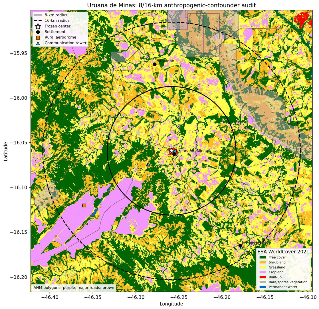
ESA WorldCover classifies only 0.458% of the frozen 8 km disk as built-up, approximately 0.92 km², while tree cover, shrubland, grassland and cropland together account for 98.67%. Expanding the screen to 16 km increases the absolute built footprint only to approximately 1.44 km² and reduces its fractional coverage to 0.179%; the same four rural/vegetated classes account for 99.10%. The urban footprint is therefore compact rather than coextensive with the magnetic target or sensitivity envelope (Fig. 15).
Official ANEEL geospatial queries return no high-voltage transmission line, transmission substation or registered generation plant within 16 km. The nearest registered generator is a 20 kW small hydropower installation 26.31 km from the frozen center. SIGMINE contains one active-process polygon inside 8 km: process 830111/2008, a 2 ha clay licensing request whose recorded filing date is 3 January 2008. Twelve additional polygons intersect the 8–16 km annulus, nine of them research authorizations; none of these legal polygons by itself demonstrates extraction, machinery or a magnetic source mass.
Supplementary mapping identifies five communication towers inside 8 km, two hamlets in the outer annulus and one rural aerodrome 12.79 km from the center, but no tagged industrial, quarry or power installation. These inventories cannot establish universal absence. They do establish a scale and chronology mismatch: point-like modern infrastructure and a 2008 licensing request cannot be the common source of a boundary geometry already present in the 1971–1972 archive, and no mapped major energy installation occupies the 16 km sensitivity envelope.
Figure 15.
Anthropogenic-confounder screen around the frozen Uruana center. Solid and dashed circles mark the pre-existing 8 km target disk and 16 km sensitivity envelope. Background colors show ESA WorldCover 2021 classes; purple polygons are active ANM mineral-process areas and do not necessarily indicate operating mines. Major roads, settlements, communication towers and the rural aerodrome are overlaid. Official ANEEL queries returned no high-voltage transmission line, transmission substation or registered generation plant within the sensitivity envelope. Present-day mapping is not interpreted as a reconstruction of 1971.
4.18. Three-Flight Finite Differences Reconstruct the Later Turnover-Front Axis
A final scalar reconstruction asks whether three independent 2008 flight intercepts recover the orientation of the later front. The standard operator gives east derivatives of +3.865 and +4.157 nT km−1 from reciprocal lines 10 and 20 and a north derivative of +2.001 nT km−1 from tie-line 9120. Their mean defines a horizontal raw scalar-gradient estimate of 4.482 nT km−1 at 63.488°. One uniform-regional 2011 endpoint definition is 63.503°, a nominal 0.015° difference. Because a second frozen implementation and PCA descriptions also exist, this pairing is not treated as mapping accuracy; Section 4.19 reports the full operator envelope. The estimate describes finite-support derivatives of scalar magnitude, not the magnetic-field-vector direction.
When the standard reciprocal operator is translated in paired 1-km increments, the Uruana corridor has the smallest endpoint-front mismatch among 201 positions within ±100 km. This rank is descriptive because the target tie-line north component is retained and the test was designed after the front was known. It nevertheless shows that the closure is spatially attached to the selected corridor rather than produced by an arbitrary east-gradient value elsewhere on the two lines.
The raw-field scalar-gradient estimate also closes against the processed representation. The IGRF14 scalar-gradient estimate is (+0.569 E,+1.096 N) nT km−1; subtracting it from the observed estimate gives (+3.441,+0.904) nT km−1 at 75.275°. An independent reconstruction from archived processed-anomaly steps gives (+3.478,+0.948) nT km−1 at 74.760°. The axes differ by 0.515° and the estimate gap is 0.0566 nT km−1, 1.57% of the processed magnitude. Because both representations derive from the same 2008 survey, this is a scalar processing-consistency closure rather than independent geological evidence or a geographic magnetic-vector reconstruction. Figure 16 summarizes the three-flight scalar-gradient closure.
4.19. The Reversal Is a Spatially Coherent Directional-Derivative Front
The crustal-overmatch ratio exceeds the reversal threshold in the target on 14/14 lines (R=1.234-5.204) and falls below it in the same-line northern controls on 14/14 lines (R=-1.087 to 0.744). Raw target slopes are negative, raw northern slopes are positive and IGRF slopes remain positive in both zones on every line. Smooth-field behavior therefore requires at least one dT/dN=0 crossing between the zones on each line. The breakpoint chains estimate the spatial organization of those crossings; they are not direct pointwise zeros.
The exact frozen 2011 breakpoint chain gives endpoint and PCA axes of 61.776 and 63.688 degrees; the independently archived uniform regional implementation gives 63.503 and 65.511 degrees. The nine 2008 three-flight estimates span 63.318-63.557 degrees. All 36 window-by-front comparisons lie within 2.193 degrees. Under the uniform endpoint operator, Uruana is the closest of the six strict 2011 centers to the fixed 2008 target axis. Thus the earlier 0.015-degree nominal pairing is one member of a broader multidefinition angular agreement, not the promoted accuracy claim. The independent 2008 + - + + interval topology further brackets a finite negative-derivative domain. The complete front-orientation mismatch envelope is shown in Figure 17.
4.20. The Complete Uruana Architecture Is Documentarily Rare
The screen recovered several relevant comparator classes but no full documentary analogue. Bangui is a long-wavelength crustal anomaly supported by satellite, airborne, ground-magnetic and gravity observations (Regan & Marsh, 1982), whereas Kursk has been outlined using satellite-altitude horizontal magnetic gradients over approximately 190,000 km² (Taylor et al., 2014). The Jõhvi anomaly is a compact, high-amplitude iron-ore case controlled by subvertical remanent magnetization (Plado et al., 2020). German repeat stations support regional vector crustal-anomaly maps at approximately 37 km resolution (Korte & Thébault, 2007). Scalar–vector aeromagnetic equivalence has been tested over an overlapping survey area (Gavazzi et al., 2020), and a modern towed vector system demonstrates both the value of simultaneous measurements and their sensitivity to orientation uncertainty (Freiman & Granot, 2025). None reports the full Uruana conjunction: all-line raw-gradient opposition to IGRF, same-line recovery, stable opposed-wall midpoint geometry across two earlier epochs, reciprocal-heading persistence, scalar–triaxial magnitude agreement and approximately four decades of recurrence. The rarity claim concerns this documented architecture, not the universal absence of analogous but unreported anomalies.
5. Discussion
5.1. What Is Exceptional at Uruana: A Locked Frame Under Spectrum Change
The central result is not one extreme rank or one fitted angle. It is the survival of the same geographic organization while the survey, sensor, processing, support and curvature state change. In 2011, every usable line reverses the positive main-field expectation inside the target and recovers farther north. In 1971–1972 and 2008, independently reconstructed Hessians preserve nearly the same signed frame and saddle topology even though eigenvalue dominance and derived vertical scalar curvature change sign. The organizing directions remain nearly fixed while the measured state changes. That frame–state separation, extended by the 2011 front, is what gives the anomaly its four-decade identity.
5.2. The Partial Envelope Is the Observation; a Closed Dome Is a Hypothesis
The opposed walls change the interpretation from a single edge to a bilateral object. Independent reconstructions place Uruana within 0.162 km of the historical midpoint and within 0.300–1.207 km of the modern midpoints. Their common 21–30° axial interval and the canonical 0/407 control result make the geometry more specific than either epoch alone. The eight occasional near-matches cluster in one 23.199° sector, but that concentration was characterized after the sweep and remains descriptive because the footprint-conditioned reference does not preserve spatial dependence.
The treatment structure points in the same direction without adding an independent test. All 36 historical–modern pairings that use the corrected 2008 field at 3.0 or 4.5 km smoothing have no exceeding control; the occasional competitors occur only in raw-field or least-smoothed treatments. Because the historical walls appear only after restoration of the main-field gradient, the measured object is the derivative geometry created by the superposition of broad main-field and local crustal contributions.
The observed envelope consists of opposed, persistent and spatially selective directional-derivative walls whose midpoints remain near Uruana. It is legitimate to call them magnetic-gradient walls because the sign transition and bilateral parity are measured and reproduced. Zero winding rejects the simplest centered scalar maximum or minimum, but that negative test concerns closure of a static horizontal scalar map. It does not test a non-axisymmetric vector envelope whose closure would depend on direction, height or time. The reciprocal and tangential results make that distinction physically relevant without completing it. A closed magnetic dome therefore remains a live, falsifiable hypothesis. Resolving it requires complete azimuthal sampling, measured vertical continuity and attitude-calibrated geographic derivatives. The surviving three-dimensional alternatives and their discriminating measurements are summarized in Figure 18.
5.3. What the Recovered Triaxial File Establishes
The recovered file closes the strongest remaining single-channel and monotonic-drift alternatives. Scalar mag1 and the Euclidean norm of three simultaneous fluxgate axes use different measurement architectures, yet they recover both the reciprocal east–west contrast and the cross-line south-to-north deficit. The latter residuals differ by only 0.015390 nT km−1, or 0.730%, inside a target fixed without using the recovered file. Reversing the flight heading also reverses acquisition order without reversing the geographic contrast.
This is a nuisance-coordinate falsification chain rather than an independent-platform replication. Sensor representation, heading and acquisition order change, while the scalar-magnitude response remains attached to the same geographic sector; an orthogonal traverse acquired 63 days earlier rises toward the same fault side. Shared aircraft and survey time remain limitations. Heading remains aliased with line identity, but the combined evidence rejects an effect confined to one scalar recording path, one heading or one survey generation. Across these heterogeneous archives, geometry is more reproducible than absolute amplitude.
The stored axes impose an equally important inferential boundary. Raw fZ is not geographic vertical, true roll and pitch are unavailable, and the fZ-exclusive hypothesis fails. The reciprocal construction nevertheless recovers same-sense inclination steps on both traverses, and the latitudinal decomposition remains more than 99.88% tangential under five target-excluding calibrations. Approximate GPS+IGRF calibration preserves the directional rate but fails Maxwell cross-derivative consistency in all 36 reconstructions. The archive therefore establishes conditional sensor-frame reciprocal inclination bending and predominantly tangential organization; it does not yet establish a geographic tensor, field-line rotation, vortex or dome.
Two levels of invariance emerge when the triaxial and Hessian results are read together. In sensor space, scalar mag1 and the rotation-invariant fluxgate norm recover the same boundary while empirical vector alignment places most of the residual derivative perpendicular to the regional field. In geographic derivative space, the 1971 and 2008 principal frames rotate by only 3.328° even though eigenvalue dominance and derived vertical scalar curvature change sign. Location, boundary and organizing frame persist while channel, waveform, amplitude and curvature state change. This convergence is a synthesis of dependent observations, not a new probability or proof of three-dimensional closure.
5.4. Static Scalar Closure and Dynamic Vector Closure Are Different Hypotheses
A static scalar dome predicts closed horizontal contours or nonzero winding in one epoch; that model fails in 89/90 contour representations and at every tested winding radius. A dynamic vector-envelope hypothesis predicts coherent directional organization, reciprocal inclination bending, tangential deflection and temporal evolution. The archive contains the first three as conditional sensor-frame spatial signatures, but it cannot identify temporal motion because acquisition date, flight line and position are confounded. Dynamic behavior remains an admissible and testable source model, not an observation.
The failed scalar-contour test does not reject every non-axisymmetric vector envelope, and the directional deflection does not establish circulation or shielding. Altitude decay and missing geographic closure prevent any regional protective claim. A dedicated campaign must recover geographic vectors around the full target, at multiple heights and simultaneous times, and satisfy Maxwell consistency before circulation, three-dimensional closure or protective function can be evaluated.
5.5. A Stable Boundary Does Not Require a Stable Waveform
The failed reciprocal waveform test is a discriminator, not an embarrassment. If one compact source body dominated both adjacent crossings, the linearly detrended geographic profiles should retain a similar shape. Instead they anticorrelate while producing nearly equal two-sided contrasts. The parsimonious inference is a boundary between crustal domains whose internal magnetization state varies along strike. This is independently consistent with the multiepoch Hessian result: eigenframe orientation changes by only 3.328° between 1971 and 2008 while the normalized eigenvalue spectrum changes strongly. Location and frame persist; detailed waveform and curvature state do not.
Several physical source classes remain compatible with that geometry, including juxtaposed magnetization domains, a remanently magnetized structural block, a fault-damage or alteration zone, and interacting edges at different depths. The available scalar fields do not uniquely distinguish them. The BU371 occurrence makes the short São Domingos segment an unusually concrete target for field tests, but hematite is neither necessary nor demonstrated as the source.
5.6. Convergent Falsification Isolates the Surviving Source Class
Table 6 compares the surviving source class against the principal alternatives and falsification controls.
The intersection of these controls isolates a spatially fixed crustal magnetic-property boundary as the surviving explanatory class. It does not isolate one mineralogical mechanism: susceptibility contrast, remanent magnetization, fault-zone alteration and interacting boundaries at depth remain distinguishable only by new ground and attitude-corrected vector measurements.
The environmental screen independently narrows the anthropogenic alternative. The 8 km target disk contains less than 0.5% built-up cover, and no registered major power asset occurs within the 16 km sensitivity envelope. The only mineral-process polygon inside the target is a 2 ha clay licensing request filed in 2008, whereas the recovered boundary geometry is already present in 1971–1972. These facts strongly disfavor major urban, industrial, mining or energy infrastructure as the common cross-epoch cause. They do not rule out isolated local contamination by fences, vehicles, distribution wiring or unmapped objects; such sources remain relevant to point-scale observations but do not match the observed spatial and temporal architecture.
5.7. A Finite-Width Reversal Domain with Cross-Epoch Boundary Registration
The 2011 lines establish a directional-derivative recovery front, while the independent 2008 + − + + sequence establishes a bounded negative-derivative interval. The 2008 field also contains ordered phase changes near 6 km (HEN=0), 12–13 km (first det(H)=0) and 19–20 km (second det(H)=0). The outer family is not merely in the same radial regime: all six channel-by-support roots lie within 0.702 km of the frozen 2011 PCA line, with a mean absolute perpendicular separation of 0.358 km. At the frozen orientation, the observed front is the best of 65 translated parallel positions under both fixed distance scores.
That rank supplies a positional denominator, not a p-value or a test of orientation. The antipodal analysis independently adds a 7–9 km bilateral boundary whose midpoint remains near Uruana in 1971–1972 and 2008. The distances are not treated as literal concentric shells. Their ordered recurrence and cross-epoch registration instead provide quantitative constraints that any future closed-envelope model must reproduce.
Taken together, these observations define a multilevel scalar-field architecture rather than a single peak or edge: a persistent saddle-organized frame, a bounded meridional negative-gradient domain, opposed directional-derivative walls and an ordered sequence of curvature transitions. The outer 2008 Hessian-degeneracy family registers to the independently recovered 2011 front, while saddle topology survives all 100 upward-continuation realizations. These relationships establish nested sampled-field geometry and a cross-epoch outer boundary, not concentric physical shells or three-dimensional closure.
5.8. The Structural Map Supplies an Empirical Natural Coordinate Frame
The most physically interpretable result is the near-diagonalization of H after rotation into the mapped structural frame. Any symmetric Hessian can be diagonalized by choosing its own eigenvectors; that would be tautological. Here the rotation angle is supplied externally by mapped structural grain. The strong reduction of the mixed term therefore tests whether geological orientation approximates the magnetic eigenframe. Its persistence in a historical Hessian and across a 2008 scale family indicates that the relation is not restricted to one processed grid or one support radius.
This result establishes the natural geometric frame without yet selecting its physical cause. The paper asks where the natural axes of the scalar field lie and how stably they are recovered, not what process generated the magnetic properties.
5.9. From Retrospective Alignment to Held-Out Cross-Domain Consistency
Alignment alone is vulnerable to a natural criticism: in a region with repeated structural trends, one may find a similar geological strike after inspecting the magnetic eigenframe. The empirical wrong-fabric substitution test directly targets that possibility. It does not compare Uruana with arbitrary continuous angles; instead it supplies the fixed Uruana Hessian with the 28 structural axes actually observed in the regional geology set. The geographically correct Uruana fabric is the best of those 28, which gives the structural frame empirical specificity beyond a generic regional strike family.
The leave-one-domain-out tests provide a more stringent test of cross-domain angular consistency than a single pairwise alignment, because each domain is withheld in turn rather than included in a fitted common orientation. In the three-domain test, every pair among 1971 magnetics, 2008 magnetics and geology reconstructs the third; Uruana's worst error is 2.29 deg, whereas the next regional center exceeds 24 deg. Adding the 2011 front normal enlarges the error, as expected for a transverse turnover boundary recovered by a different survey operator, but the four-domain angular consistency remains the best of nine complete centers. These are post-discovery internal holdout consistency tests, not out-of-sample prediction of a previously unseen dataset.
5.10. Frame and State Are Separable Observables
The west-to-Uruana sign flip clarifies the physical meaning of the eigenframe result without selecting a cause. Two neighboring centers can share nearly the same mapped structural orientation while assigning opposite curvature signs to that direction. The reference frame is therefore not synonymous with the local magnetic state. This separation explains how a long-lived structural coordinate system can coexist with spatially varying scalar-field behavior and with a 2011 turnover that is approximately transverse to the frame.
This frame-state distinction also explains why eigenvector persistence can survive eigenvalue-spectrum change. A persistent frame does not require the ratio or amplitude of principal curvatures to remain fixed; it requires the directions organizing those curvatures to remain recoverable. At Uruana, the branch-dominance exchange forces the horizontal trace, and therefore the derived vertical scalar curvature, through a sign change while the principal axes rotate by only 3.328 deg. The upward-continuation result extends frame persistence into vertical scale-space, whereas the failed scale-flow smoothness screen prevents us from claiming that every aspect of the frame evolves unusually smoothly with scale.
The external Alaska control separates operator generality from local exceptionalism. It prospectively confirms recoverability of an unsigned eigenframe across heterogeneous archives under adequate spatial support; it does not reproduce Uruana's signed branch, gradient reversal or spectrum-state change. General operator recoverability and the specific Uruana architecture are therefore distinct claims.
5.11. Rarity Is Repeated Survival, Not Multiplication of Ranks
The regional screens are intentionally heterogeneous. A 1/231 affine-row rank, a 1/28 signed-frame rank and a 1/28 structural-alignment rank share data and cannot be multiplied. Likewise, nested-phase, tri-epoch and leave-one-domain-out screens use overlapping representations. Because these screens share data, their evidential weight is robustness-based rather than multiplicative: together, they establish that Uruana repeatedly occupies an extreme or surviving regional position under distinct, mechanically specified transformations of the same archives. Wrong-fabric substitution, held-out-domain reconstruction, eigenvalue-sign retention and vertical scale-space are especially useful because they probe different failure modes rather than adding interchangeable ranks.
5.12. Documentary Rarity Without Worldwide Overclaim
Within the searched literature, Uruana is the first documented case of this complete observational conjunction. The claim is deliberately architecture-specific. Local derivatives can change sign around many magnetic sources, and comparable behavior may remain unreported in legacy, non-English, proprietary or unindexed datasets. What is presently without a published analogue is the combined kilometre-scale localization, opposed-wall midpoint stability across epochs, same-line recovery, three survey generations, reciprocal headings, two measurement architectures, approximately four decades of recurrence and an independently mapped structural frame. A single earlier publication satisfying that conjunction would falsify the documentary-primacy statement.
5.13. A Closed Three-Dimensional Envelope Is Now a Decisive Falsifiable Hypothesis
The observations elevate three source classes for direct comparison (Fig. 18). A closed shell or non-axisymmetric dome could intersect the available flight geometry as opposed scalar-gradient walls, but it must additionally predict azimuthal closure, systematic evolution with observation height and attitude-calibrated geographic derivatives consistent with Maxwell constraints. A dipping fault or alteration boundary predicts elongation along structural strike and need not close around the city. Juxtaposed magnetization domains or interacting sources can explain waveform anticorrelation and persistent structural axes but likewise need not form a closed surface. Existing scalar archives distinguish the partial envelope from a single-line artifact; they do not yet discriminate these three-dimensional models.
The decisive campaign is therefore specific. Orthogonal and oblique flight lines should sample the full 360° annulus at multiple heights, while calibrated ground-vector profiles cross the 7–9 km walls and the outer 12–20 km transitions. Continuous magnetometers should operate simultaneously inside the envelope, on the observed walls and at a control beyond 20 km. Such a design would test spatial closure, vertical continuity, temporal coherence and any claimed local effect. Biological, atmospheric, technological or protective effects are not inferred from the present archive; they require independently defined response variables and simultaneous inside–outside controls.
5.14. Limitations, Procedural Genealogy and Future Falsification
Several analyses were developed after discovery and are labeled accordingly. The 1971 observations are sparse residual products; the 2008 grid and original-file profiles have different supports; and the 2011 survey does not sample every direction equally. Fitted breakpoints localize turnover but are not direct pointwise measurements of dT/dN=0. Two archived implementations differ, so front orientation is promoted only as the four-definition envelope. Scalar and fluxgate data share one aircraft; roll, pitch and mounting are unavailable; and Maxwell closure fails. Upward continuation is a scale operator rather than an altitude measurement: the central saddle persists, but the external root migrates and vanishes. The three-dimensional models remain hypotheses, not inversions.
6. Conclusions
The result begins with the least model-dependent observation in the study. On every usable 2011 flight line, the measured northward total-field gradient is negative inside the +6 to +8 km target cap although the IGRF gradient is positive; farther north, the measured gradient returns to positive. All 14 paired control-minus-target residual contrasts have the same sign. The frozen breakpoint chain organizes those line-wise recoveries into a front. When this complete signature is intersected with the independent bounded + − + + topology of the 2008 grid, Uruana is the sole joint pass among 82 commonly supported regional centers.
The older archives show that this is not a feature of one survey product. Historical 1971–1972 and modern 2008 reconstructions recover opposed directional-derivative walls in the same 7–9 km annulus and place their midpoints near Uruana. The recovered original 2008 file preserves the same geographic contrast in a scalar magnetometer and in the rotation-invariant norm of a triaxial fluxgate, even when reciprocal flight direction reverses acquisition order. Conditional sensor-frame analyses further recover same-sense inclination bending and a residual derivative that remains more than 99.88% tangential across five calibrations. These directional results do not establish absolute geographic vector components.
The most persistent observable is the frame. Historical and 2008 eigenaxes align with the independently mapped structural grain, and the correct local fabric outperforms every wrong regional fabric supplied to the fixed Uruana Hessian. When 1971 magnetics, 2008 magnetics and geology are reconstructed one domain at a time, Uruana has a 2.287° worst held-out error; the next regional center exceeds 24°. The frame survives even as waveform, amplitude, eigenvalue dominance and derived vertical scalar curvature change. Uruana therefore preserves an organizing coordinate system rather than a stationary magnetic state.
These independent views resolve one coherent architecture: a bounded gradient reversal, a persistent bilateral midpoint, a structurally locked frame and a native-scale outer boundary registered across epochs. All six 2008 outer roots lie within 0.702 km of the frozen 2011 PCA front, which ranks first among 65 parallel translations. Under upward continuation, the central saddle persists in 100/100 realizations to 12 km, while the external root migrates and disappears by approximately 4 km at standard support. The contrast separates a stable central topology from a scale-dependent external boundary; it does not convert continuation height into source depth.
The geographic and chronological controls point away from a common acquisition or infrastructure explanation. The target contains only 0.458% built-up cover inside 8 km, has no registered major power infrastructure inside 16 km, and preserves related geometry in survey generations separated by approximately four decades. Within the explicitly searched literature, no published analogue combines this same cross-epoch, cross-instrument, reciprocal-heading and structurally registered architecture. The claim is documentary and conjunction-specific, not a statement of worldwide physical uniqueness.
The remaining question is what three-dimensional object can generate the measured architecture. Approximate GPS+IGRF calibration preserves the directional rate, but none of 36 reconstructions satisfies the illustrative Maxwell band. A closed shell, a non-axisymmetric or dynamic dome, a dipping structural boundary, and juxtaposed magnetization domains therefore remain competing hypotheses. Closure must be tested with full-azimuth sampling, measurements at multiple heights, simultaneous observations and attitude-calibrated geographic vectors. Circulation, shielding and atmospheric protection likewise remain unresolved until those tests exist. The paper establishes the persistent partial envelope; it leaves its possible closure open in a form that can now be falsified.
Data Availability Statement
All primary empirical data originate from public Brazilian geophysical archives and public geological mapping. Large upstream archives are not redistributed. Supplementary File S2 supplies source identifiers, checksums, derived line and control tables, the antipodal-envelope audit, the rotation-invariant latitudinal audit, the negative Maxwell-closure result, the 8/16 km anthropogenic-confounder audit, figure-source data and deterministic verification code.
Conflicts of Interest
The authors declare no conflicts of interest.
Author Contributions
LGR: conceptualization, methodology, software, formal analysis, investigation, data curation, visualization, writing - original draft, and project administration. MAS: methodology, validation, formal analysis, investigation, and writing - review and editing. Both authors reviewed and approved the final manuscript and are accountable for the work.
Funding
The authors declare that no funds, grants, or other support were received during the preparation of this manuscript.
Acknowledgments
The authors thank the Ágora Study Group, based in Uruana de Minas, for discussion and intellectual exchange. OpenAI ChatGPT was used only for the limited assistance disclosed in Sect. 3.11. All scientific conception, methodological and inferential choices, data verification, validation, interpretation and final decisions were performed and approved by the authors, who retain full responsibility. No generative-AI images were used.
Supplementary Materials
The following supporting information can be downloaded at the website of this paper posted on Preprints.org. Supplementary Materials. ZIP. Supplementary File S1 provides extended methods, sensitivity analyses, negative results and model predictions. Supplementary File S2 provides machine-readable source tables, claims matrices, deterministic code, vector and Maxwell audits, vertical root tracking, the scale-space bifurcation surface, the angular-frame inventory and altitude-decay calculations.
References
- Agência Nacional de Energia Elétrica (ANEEL) (2026a) SIGEL geospatial transmission-line and substation services. https://sigel.aneel.gov.br/. Accessed 11 Sep 2026.
- Agência Nacional de Energia Elétrica (ANEEL) (2026b) SIGA: Sistema de Informações de Geração da ANEEL. https://dadosabertos.aneel.gov.br/dataset/siga-sistema-de-informacoes-de-geracao-da-aneel. Accessed 11 Sep 2026.
- Agência Nacional de Mineração (ANM) (2026) SIGMINE: Processos minerários ativos. https://geo.anm.gov.br/arcgis/rest/services/SIGMINE/dados_anm/MapServer/0. Accessed 11 Sep 2026.
- Agência Nacional do Petróleo, Gás Natural e Biocombustíveis (ANP) (2008) Acervo de dados técnicos não sísmicos: Projeto 0032 São Francisco. ANP, Brazil.
- Alkmim FF, Martins-Neto MA (2012) Proterozoic first-order sedimentary sequences of the São Francisco craton, eastern Brazil. Mar Pet Geol 33:127-139. [CrossRef]
- Beamish D, White JC (2011) Aeromagnetic data in the UK: a study of the information content of baseline and modern surveys across Anglesey, North Wales. Geophys J Int 184:171-190. [CrossRef]
- Beggan CD et al (2026) International geomagnetic reference field: the fourteenth generation. Earth Planets Space 78:127. [CrossRef]
- Brown PJ (2009) Aeromagnetic survey of Howard Pass quadrangle and the east half of Misheguk Mountain quadrangle, Alaska - a Web site for the distribution of data. U.S. Geological Survey Open-File Report 2009-1256. [CrossRef]
- CODEMIG/UFMG (n.d.) Projeto Fronteiras de Minas Gerais: Folha Buritis SD.23-Y-D-IV, mapa geológico, relatório e SIG, escala 1:100,000. Belo Horizonte, Brazil.
- Connard GG, Saltus RW, Hill PL, Carlson L, Milicevic B (1999) Alaska digital aeromagnetic database description. U.S. Geological Survey Open-File Report 99-503. [CrossRef]
- Estado de Minas Gerais (1995) Lei nº 12.030, de 21 de dezembro de 1995. Assembleia Legislativa do Estado de Minas Gerais. https://www.almg.gov.br/legislacao-mineira/LEI/12030/1995/.
- Freiman S, Granot R (2025) AeroVmag: A new aero-towed vector magnetometer system. Geophysics 90:G139-G150. [CrossRef]
- Gavazzi B, Bertrand L, Munschy M, Mercier de Lépinay J, Diraison M, Géraud Y (2020) On the use of aeromagnetism for geological interpretation: 1. Comparison of scalar and vector magnetometers for aeromagnetic surveys and an equivalent source interpolator for combining, gridding, and transforming fixed-altitude and draping data sets. J Geophys Res Solid Earth 125:e2019JB018870. [CrossRef]
- Gibson HA, Tailleur IL (1980) Map showing relations between aeromagnetic data and geology, southern National Petroleum Reserve in Alaska. U.S. Geological Survey Open-File Report 80-516. [CrossRef]
- Guillard R, Gailler L, Labazuy P, Thebault E, Régis E, Dumont Q (2025) Insight into magmatic pathways and subsurface structures from repeated UAV magnetic prospecting at Piton de la Fournaise volcano, Réunion Island. Earth Planets Space 77:169. [CrossRef]
- Hokari T, Tanaka R, Hashimoto T, Koyama T (2026) Shallow thermal activity of Tokachidake Volcano (Japan) investigated through repeated drone-borne magnetic surveys. Earth Planets Space 78:81. [CrossRef]
- Instituto Brasileiro de Geografia e Estatística (IBGE) (2025) Uruana de Minas: Cidades e Estados. https://www.ibge.gov.br/cidades-e-estados/mg/uruana-de-minas.html. Accessed 22 Aug 2026.
- Ito R, Utsugi M (2025) New magnetic inversion scheme including terrain-effect correction. Earth Planets Space 77:176. [CrossRef]
- Johnson MR, Anderson ED, Ball LB, Drenth BJ, Grauch VJS, McCafferty AE, Scheirer DS, Schweitzer PN, Shah AK, Smith BD (2019) Airborne Geophysical Survey Inventory of the Conterminous United States, Alaska, Hawaii, and Puerto Rico (ver. 5.0, April 2024). U.S. Geological Survey data release. [CrossRef]
- Korte M, Thébault E (2007) Geomagnetic repeat station crustal biases and vectorial anomaly maps for Germany. Geophys J Int 170:81-92. [CrossRef]
- Lahti I, Karinen T (2010) Tilt derivative multiscale edges of magnetic data. Lead Edge 29:24-29. [CrossRef]
- OpenStreetMap contributors (2026) OpenStreetMap data queried through the Overpass API. https://www.openstreetmap.org/. Accessed 11 Sep 2026.
- Phillips JD, Hansen RO, Blakely RJ (2007) The use of curvature in potential-field interpretation. Explor Geophys 38:111-119. [CrossRef]
- Pilkington M, Tschirhart V (2017) Practical considerations in the use of edge detectors for geologic mapping using magnetic data. Geophysics 82:J1-J8. [CrossRef]
- Pimentel MM, Rodrigues JB, DellaGiustina MES, Junges S, Matteini M, Armstrong R (2011) The tectonic evolution of the Neoproterozoic Brasília Belt, central Brazil, based on SHRIMP and LA-ICPMS U-Pb sedimentary provenance data: a review. J S Am Earth Sci 31:345-357. [CrossRef]
- Plado J, Kiik K, Jokinen J, Soesoo A (2020) Magnetic anomaly of the Jõhvi iron ore, northeastern Estonia, controlled by subvertical remanent magnetization. Est J Earth Sci 69:189-199. [CrossRef]
- Regan RD, Marsh BD (1982) The Bangui Magnetic Anomaly: its geological origin. J Geophys Res Solid Earth 87:1107-1120. [CrossRef]
- Saltus RW, Chulliat A, Blakely RJ (2026) Evaluation of aliasing in aeromagnetic surveys - update to Reid 1980 analysis. Earth Space Sci 13:e2025EA004336. [CrossRef]
- Sertcelik I, Kafadar O (2012) Application of edge detection to potential field data using eigenvalue analysis of structure tensor. J Appl Geophys 84:86-94. [CrossRef]
- Serviço Geológico do Brasil (SGB) (2026a) GeoSGB public aerogeophysical data: Project 3087 - Area 19 - Formoso - Buritis - Lagoa Grande. https://geosgb.sgb.gov.br/downloads/. Accessed 14 Aug 2026.
- Serviço Geológico do Brasil (SGB) (2026b) GeoSGB public aerogeophysical data: Project 1009 - Projeto Aerogeofísico Convênio Brasil-Alemanha. https://geosgb.sgb.gov.br/downloads/. Accessed 14 Aug 2026.
- Taylor PT, Kis KI, Wittmann G (2014) Satellite-altitude horizontal magnetic gradient anomalies used to define the Kursk Magnetic Anomaly. J Appl Geophys 109:133-139. [CrossRef]
- Yuan Y, Huang D, Yu Q, Lu P (2014) Edge detection of potential field data with improved structure tensor methods. J Appl Geophys 108:35-42. [CrossRef]
- Yuan Y, Yu Q (2015) Edge detection in potential-field gradient tensor data by use of improved horizontal analytical signal methods. Pure Appl Geophys 172:461-472. [CrossRef]
- Zanaga D et al (2022) ESA WorldCover 10 m 2021 v200. [CrossRef]
Figure 1.
Geographic and self-contained 2011 baseline. (a) Brazil locator for Uruana de Minas; the point is the municipal-seat reference used only for geographic plotting. (b) Raw target slopes are negative on all 14 usable Project 3087 flight lines, whereas the same lines 16–20 km north are positive and IGRF medians remain positive in both zones. Median line-wise raw−IGRF residuals are −2.607 and +0.267 nT km−1; all 14 within-line control-minus-target residual contrasts are positive (median 2.922 nT km−1). The complete strict signature occurs at 6/97 regional centers. (c) Frozen negative-to-positive breakpoint chain with exact endpoint and PCA axial orientations. Country outline uses Natural Earth public-domain data; geographic coordinates are from IBGE.
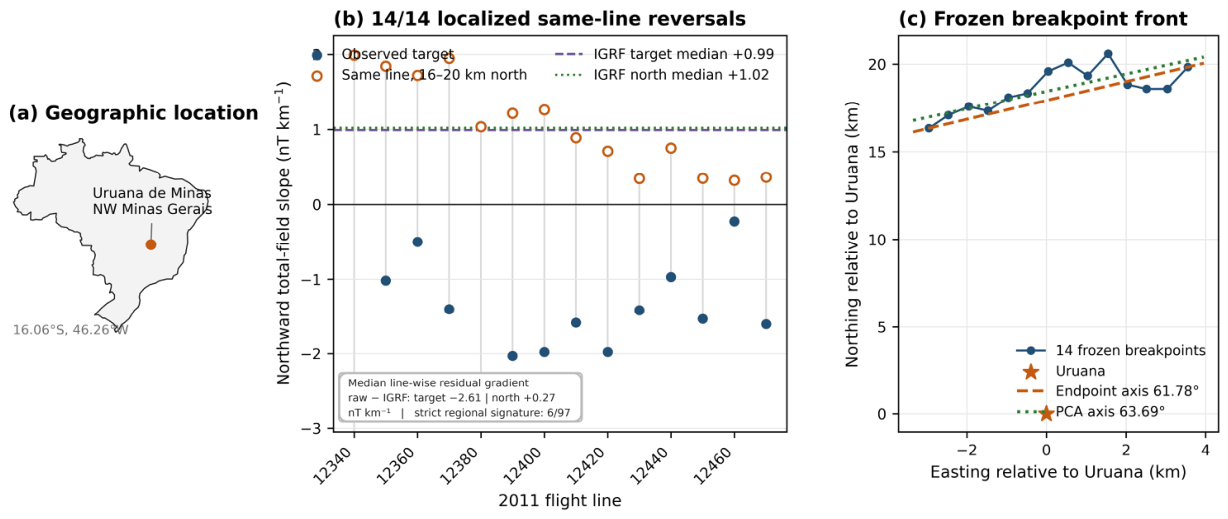
Figure 2.
Persistent opposed magnetic-gradient walls around Uruana de Minas. (a) Canonical reconstructed 1971–1972 total-field dT/dN and the fixed 8 km circle. (b) Canonical 2008 corrected-field dT/dN. Black segments mark antipodal axial intervals; black contours mark dT/dN=0. (c) The epochs overlap on ten consecutive azimuths, 21–30 degrees clockwise from north. (d) Only eight of 407 complete-support controls survive any of 108 matched specification pairs; all occupy a 23.199-degree sector containing 59/407 eligible centers. Only 9/2,000,000 random eight-center subsets achieve an equal-or-narrower optimized span in a post-discovery footprint-only reference. The strongest control survives 36/108; all 36 pairings using corrected 2008 fields smoothed at 3.0–4.5 km have zero exceeding controls. The random reference does not preserve spatial dependence and is not an anomaly p-value. Colors in (a,b) show derivative sign, not magnetic-field intensity.

Figure 3.
Independent pre-2011 geometry. (a) Historical Project 1009 E-W line slopes ordered by northing around Uruana. (b) 2008 Project 0032 northward interval gradients showing the + - + + architecture in raw and diurnal-corrected grids.
Figure 3.
Independent pre-2011 geometry. (a) Historical Project 1009 E-W line slopes ordered by northing around Uruana. (b) 2008 Project 0032 northward interval gradients showing the + - + + architecture in raw and diurnal-corrected grids.
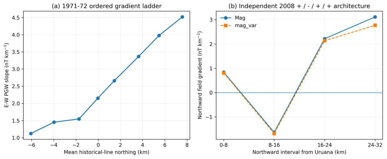
Figure 4.
Nested 2008 curvature-phase roots and cross-epoch front registration. (a) Along the fixed +2 km E track, HEN=0 occurs near 6 km, the first det(H)=0 near 12–13 km and the second det(H)=0 near 19–20 km across radii and both 2008 channels. The horizontal reference is the intersection of the independently frozen 2011 PCA front with the same track. (b) Signed perpendicular distance from each outer 2008 root to the 2011 PCA line. All six lie within 0.702 km; the mean absolute separation is 0.358 km and their mean signed position is −0.032 km. At frozen orientation, the real front ranks first among 65 translated parallel positions by both maximum and mean absolute separation. This is cross-epoch geometric registration, not evidence of a concentric shell or source depth.
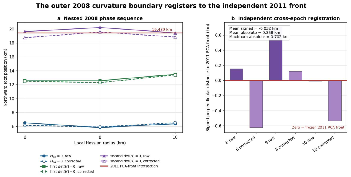
Figure 5.
Tri-epoch orientation. (a) Exact Uruana site-level positive-curvature/front axes from 1971, 2008 and the frozen 2011 breakpoint chain. (b) Regional ranking under the uniform 2011 endpoint operator; the regional operator is intentionally distinguished from the exact site geometry.
Figure 5.
Tri-epoch orientation. (a) Exact Uruana site-level positive-curvature/front axes from 1971, 2008 and the frozen 2011 breakpoint chain. (b) Regional ranking under the uniform 2011 endpoint operator; the regional operator is intentionally distinguished from the exact site geometry.
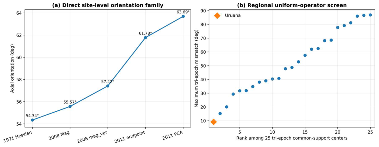
Figure 6.
Structural locking across independent orientation domains. (a) Historical 1971 and 2008 negative-curvature axes, mapped structural fabric, and normals to the exact 2011 breakpoint front occupy the same narrow axial family. (b) Mismatch between the fixed structural axis and the 2008 negative-curvature axes across 6–20 km Hessian radii; Uruana ranks 1/28 on the conservative multiscale endpoint. Panel (c) reports the frozen coordinate-referenced angular inventory; its derived sum and difference are algebraic descriptors, not independent observations.
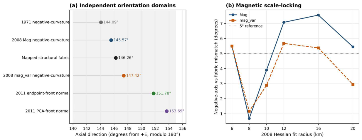
Figure 7.
Structural-frame diagonalization. (a) Geographic E,N versus structural U,V off-diagonal Hessian fractions across the 2008 scale ladder. (b) Collapse of the off-diagonal term in the 1971 historical Hessian, 2008 8-km raw/corrected Hessians and the conservative multiscale 2008 minimum.
Figure 7.
Structural-frame diagonalization. (a) Geographic E,N versus structural U,V off-diagonal Hessian fractions across the 2008 scale ladder. (b) Collapse of the off-diagonal term in the 1971 historical Hessian, 2008 8-km raw/corrected Hessians and the conservative multiscale 2008 minimum.
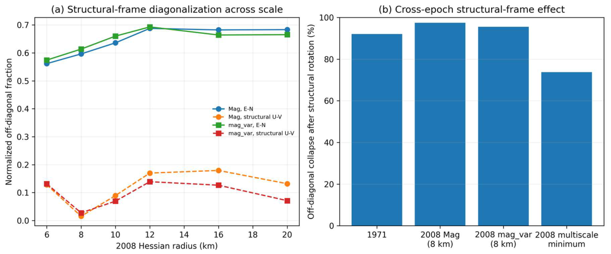
Figure 8.
Empirical wrong-fabric substitution test. The fixed 2008 Uruana Hessian is tested against all 28 mapped structural axes from the regional geology set. Uruana's own fabric produces the smallest worst raw/corrected axial mismatch (1.1597 deg); the best geographically wrong fabric gives 3.3703 deg.
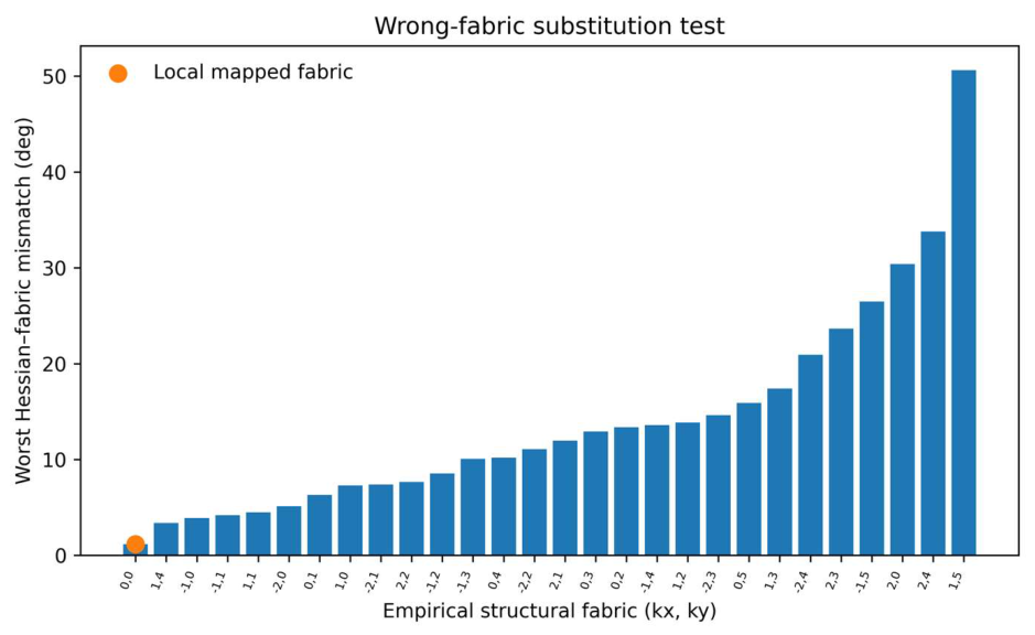
Figure 9.
Three-domain leave-one-out reconstruction. At each regional center, two of three independent orientation domains - historical 1971 Hessian, 2008 Hessian, and mapped structural grain - reconstruct the third by axial circular mean. Uruana has the smallest worst held-out error (2.287 deg) among 28 centers; the next center is 24.263 deg.
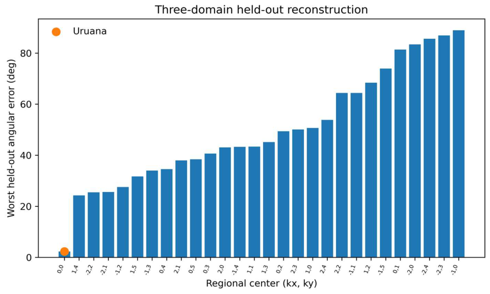
Figure 10.
Four-domain angular-consistency test. The 1971 negative-curvature axis, 2008 negative-curvature eigenframe, mapped structural axis and 2011 turnover-front normal are reconstructed leave-one-domain-out. The plotted endpoint is the conservative worst error across endpoint and PCA front descriptions; Uruana ranks 1/9.
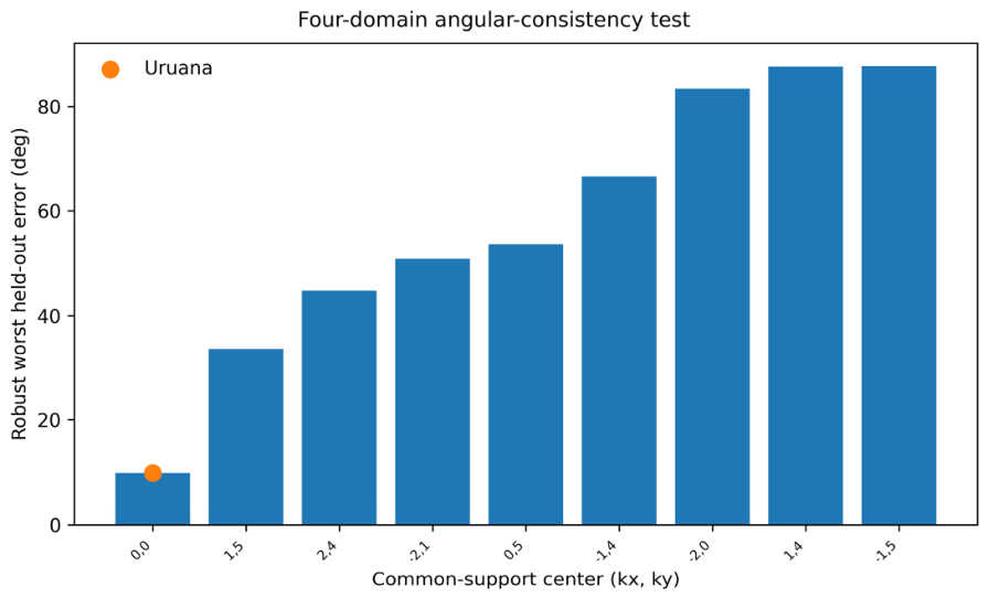
Figure 11.
Cross-epoch signed structural frame. For each geology-overlap center, the mapped structural direction is compared with the negative-curvature Hessian axis in 1971 and in 12 raw/corrected 2008 scale realizations. The plotted value is the worst mismatch across the complete family. Uruana ranks 1/28 at 7.553 deg.
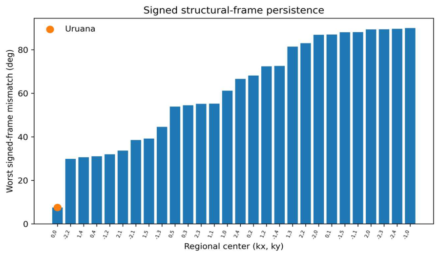
Figure 12.
Reciprocal-flight, dual-sensor audit of the recovered original 2008 file. (a,b) Scalar mag1 and rotation-invariant fluxgate-norm profiles at two fixed São Domingos crossings traversed in opposite flight directions; shading marks the side windows. (c) Both sensors retain the same fault-side increase on the reciprocal lines, while orthogonal tie-line 9120 independently reproduces that side-of-fault direction 63 days earlier. (d) Linear-background residuals do not reproduce the same local waveform. This failure distinguishes a stable boundary from a repeated compact-body fingerprint.
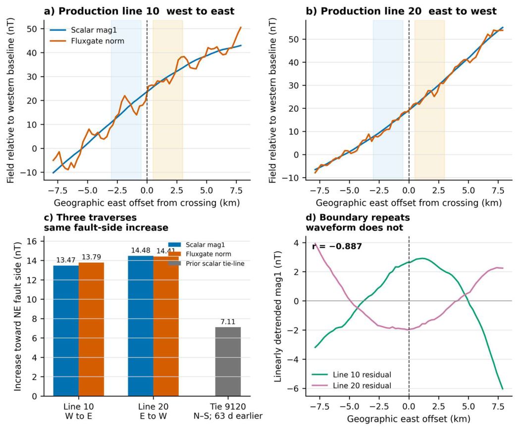
Figure 13.
Reciprocal and latitudinal vector-deflection audit. (a) After empirical reciprocal alignment, inclination steps retain the same sign on lines 10 and 20, whereas relative-declination steps oppose one another, rejecting a simple same-sense azimuthal rotation. (b) At 2–8 km support, 99.930–99.982% of the latitudinal residual derivative is tangential to the target-excluding regional field; five alternative calibrations give 99.883–99.983%. (c) Reciprocal and tangential signals survive translated and external-attitude controls, whereas 0/36 reconstructions satisfy the illustrative Maxwell closure band. Directional results remain conditional on the empirical alignment because true roll, pitch and mounting are unavailable.
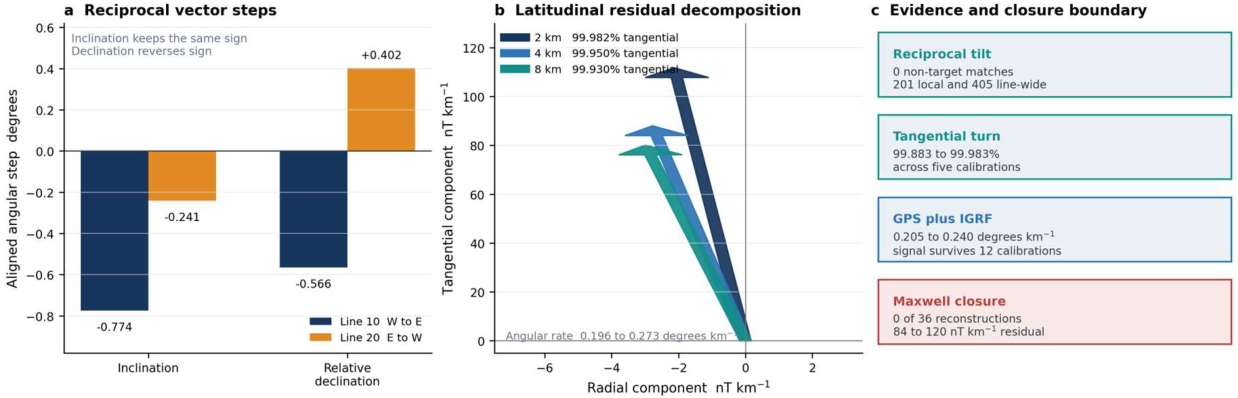
Figure 14.
Cross-epoch amplitude convergence, translated localization, along-fault concentration and 2011 crustal-gradient residual. (a) Four heterogeneous scalar observables converge at the inherited crossing. (b) Uruana ranks first for the translated three-observable spread. (c) The high response is confined to a short mapped-fault sector. (d) The median line-wise raw-minus-IGRF residual is −2.607 nT km−1 at the target and +0.267 nT km−1 in the northern same-line control; the difference between these zonal medians is 2.874 nT km−1. The distinct median of the 14 paired within-line control-minus-target residual contrasts is 2.922 nT km−1, and all 14 contrasts are positive.
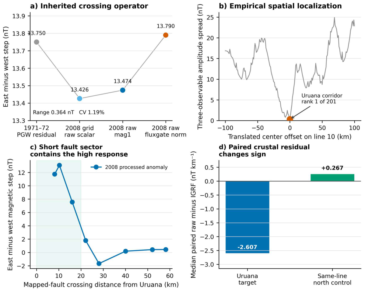
Figure 16.
Three-flight horizontal scalar-gradient closure. (a) Observed raw 2008 scalar-gradient estimate, IGRF14 estimate, raw-minus-IGRF residual and independently reconstructed processed-anomaly estimate. (b) The orthogonal tie-line combined with each reciprocal production line and their nine-window mean range. The 0.015° value is the nominal pairing with one uniform-regional endpoint definition; Figure 17 reports the complete four-definition envelope. These are derivatives of scalar magnitude, not magnetic-field-vector directions.
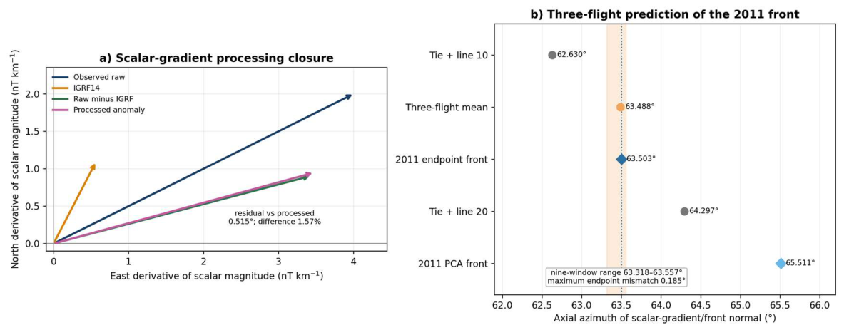
Figure 17.
Directional-derivative reversal-front audit. (a) The crustal-overmatch ratio R exceeds one in the target and returns below one in the same-line northern control on all 14 lines. (b) Exact-site and uniform-regional 2011 breakpoint operators, centered separately, with their PCA axes and the nominal 2008 three-flight scalar-gradient axis. (c) Axial mismatch for nine 2008 windows against endpoint and PCA axes from both 2011 implementations. The audit establishes a dT/dN zero-crossing front, not a stationary point of the full scalar field.
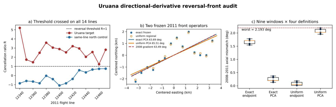
Figure 18.
From the observed partial gradient envelope to falsifiable three-dimensional models. (a) Only opposed sectors of the 7–9 km wall geometry are observed; dashed sectors are unsampled. (b) A closed shell or non-axisymmetric dome remains admissible and is prioritized for testing because it makes the sharpest falsifiable predictions; it requires azimuthal and vertical closure plus attitude-calibrated geographic vectors. (c) Dipping structural boundaries and juxtaposed magnetization domains remain competing crustal models. The lower panel specifies the measurements needed to discriminate them and to test any regional physical or temporal effect.
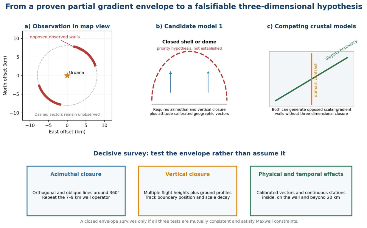

Table 1.
Datasets and inferential roles.
| Dataset | Representation | Primary role |
|---|---|---|
| 1971-72 Project 1009 | Historical PGW residual profiles, mainly E-W locally | Historical antipodal-wall holdout; line-gradient ladder; Hessian |
| 2008 Project 0032 | 1.5-km Mag and mag_var grids | Antipodal-wall replication; +/−/+ topology; Hessian; scale ladder |
| 2011 Project 3087 | Raw scalar total-field N-S flight lines + IGRF | Direct gradient reversal; free turnover front; regional strict gate |
| Buritis 1:100,000 GIS | Mapped S-surface traces + contractional/reverse faults | Independent structural grain and scale tests |
| SRTM / gravity / gamma products | Independent cross-domain fields | Negative controls and inference boundary |
| WorldCover / ANM / ANEEL / OSM | 10 m land cover and mapped infrastructure | Independent 8/16 km anthropogenic-confounder screen |
Table 2.
Cross-domain held-out reconstruction tests.
| Cross-domain holdout test | Uruana result | Comparator | Interpretation |
|---|---|---|---|
| Wrong-fabric substitution | own fabric mismatch 1.1597 deg | best wrong fabric 3.3703 deg; own fabric rank 1/28 | Geographically correct structural axis is specifically reconstructive |
| Three-domain leave-one-out | worst held-out error 2.287 deg | next regional center 24.263 deg; rank 1/28 | 1971, 2008 and geology mutually reconstruct one another |
| Four-domain leave-one-out | robust worst error 9.899 deg | next complete center 33.759 deg; rank 1/9 | Four-domain angular consistency persists after adding the 2011 turnover-front normal |
Table 3.
Regional endpoint and control summary.
| Endpoint | Uruana result | Regional reference | Status |
|---|---|---|---|
| 2011 strict raw signature | 14/14 local; 6/97 regional strict | 97 2011 candidates | Foundational / descriptive |
| 2011 strict + robust 2008 | 1/82 Uruana only | 82 common-support centers | Descriptive regional |
| 1971 gradient ladder | strict; all-line median |r| 0.9964 | 3/108 centers strict; 2/108 centers high-coherence | Exploratory |
| 2008 affine rows | worst row |r| 0.9964 | rank 1/231; only center with all rows |r| >= 0.995 | Exploratory |
| Nested phases + hist. shear + 2008 turnover | Uruana only | 1/39 ordered centers | Exploratory conjunction |
| Tri-epoch eigenframe | rank 1 under endpoint and PCA | 25 common-support centers | Exploratory |
| Positive mixed + saddle + strict 2011 | Uruana only | 1/25 | Exploratory conjunction |
| Structural alignment | 1.1597 deg | rank 1/28 | Exploratory cross-domain |
| Geological scale locking | worst 2.586 deg; min R_ax 0.630 | rank 1/23 on both | Exploratory |
| Magnetic scale locking | worst 7.553 deg | rank 1/28 | Exploratory |
| 1971 + 2008 structural diagonalization | Uruana only | 1/28 | Exploratory cross-epoch |
| Wrong-fabric substitution | own mapped fabric is best empirical axis | 1/28 fabrics as good or better | Cross-domain robustness |
| Three-domain LOO reconstruction | worst held-out error 2.287 deg | rank 1/28; next 24.263 deg | Held-out reconstruction |
| Four-domain angular LOO | robust worst error 9.899 deg | rank 1/9; next 33.759 deg | Held-out reconstruction |
| Cross-epoch signed structural frame | worst mismatch 7.553 deg; same negative-curvature branch | rank 1/28; 3/28 broad signed-frame passes | Core geometric |
| 1971–2008 antipodal envelope | 12 historical; 18 modern; midpoint offsets 0.162 and 0.300–1.207 km | canonical 0/407; corrected 3–4.5 km: 0 controls in 36/36 pairs; best overall control 36/108 specification pairs | Post-discovery cross-epoch and specification robustness |
Table 4.
Three-traverse 2008 acquisition closure and scalar–fluxgate audit.
| Sampling/operator | Scalar step (nT) | Fflux step (nT) | Inference |
|---|---|---|---|
| Line 10; west to east | +13.474 | +13.790 | same geographic sign |
| Line 20; east to west | +14.482 | +14.412 | same geographic sign |
| Tie-line 9120; north–south; 63 d earlier | +7.110 | not available | same NE fault-side increase |
| Line 10; 18 fixed variants | positive 18/18 | positive 18/18 | sampling/window robustness |
| Local translated controls | 95.3rd percentile | 95.3rd percentile | line-10 selectivity |
Table 5.
Four-stage directional and physical-closure audit.
| Stage | Quantitative result | Adjudication | Boundary |
|---|---|---|---|
| Bilateral walls | Near-north peak separation 1.75°; same-direction parity 12/12 historical, 9/9 raw 2008 and 18/18 corrected 2008 | PASS | Directional-derivative boundary; not a closed shell |
| Reciprocal bending | Inclination −0.774° and −0.241°; no non-target matches under the joint signed-component threshold | PASS conditional | Empirical reciprocal frame; absolute attitude unavailable |
| Tangential turn | Scalar–norm residual disagreement 0.730%; tangential fraction 99.883–99.983% across calibrations | PASS conditional | Direction change supported; geographic tensor unresolved |
| Maxwell closure | Cross-derivative residual 84–120 nT km−1; 0/36 within ±5 nT km−1 | UNRESOLVED | Current archive cannot establish a closed vortex or dome |
Table 6.
Alternative-explanation matrix. Each row is adjudicated by a distinct control; statuses are not multiplied as probabilities.
Table 6.
Alternative-explanation matrix. Each row is adjudicated by a distinct control; statuses are not multiplied as probabilities.
| Alternative | Decisive observation | Status |
|---|---|---|
| Smooth main-field gradient | IGRF positive in both zones; all 14 paired recovery contrasts positive; median 2.922 nT km−1 | rejected |
| Single scalar recording path | Simultaneous fluxgate norm reproduces both reciprocal crossings; scalar–norm mismatch is 2.32% and 0.49% of the respective common responses | rejected |
| Monotonic temporal drift | Opposite acquisition order preserves the geographic sign; a monotonic drift would have to reverse from +0.178 to −0.177 nT s−1 | simple monotonic drift rejected; separable heading effect unresolved |
| One flight or one-day disturbance | Orthogonal tie-line 9120 repeats the increase toward the same fault side 63 days earlier | rejected |
| Height or terrain-clearance mimic | mean-height steps are small, but the GPS flight-path-angle proxy is non-negligible | mean-height mimic rejected; attitude unresolved |
| Gridding or processing creation | original 2008 mag1/Fflux and original 2011 raw lines retain the signal | rejected |
| Mapped surface contact | strongest crossings retain the same mapped unit on both sides | not required |
| Bulk-density anomaly | Bouguer response changes sign and is stronger where magnetics are weak | not supported |
| Repeated compact body | adjacent linearly detrended waveforms anticorrelate | not supported |
| Major urban or energy infrastructure | Built-up cover 0.458% inside 8 km; no ANEEL high-voltage line, transmission substation or generation plant inside 16 km | strongly disfavored |
| Operating mine or industrial source | Only internal ANM polygon is a 2 ha clay licensing request filed in 2008; 1971–1972 geometry predates it | rejected as common cross-epoch cause |
Disclaimer/Publisher’s Note: The statements, opinions and data contained in all publications are solely those of the individual author(s) and contributor(s) and not of MDPI and/or the editor(s). MDPI and/or the editor(s) disclaim responsibility for any injury to people or property resulting from any ideas, methods, instructions or products referred to in the content. |
© 2026 by the authors. Licensee MDPI, Basel, Switzerland. This article is an open access article distributed under the terms and conditions of the Creative Commons Attribution (CC BY) license (http://creativecommons.org/licenses/by/4.0/).
Copyright: This open access article is published under a Creative Commons CC BY 4.0 license, which permit the free download, distribution, and reuse, provided that the author and preprint are cited in any reuse.