
Submitted:
14 September 2026
Posted:
15 September 2026
You are already at the latest version
Abstract
Computational Scattered Light Imaging (ComSLI) exploits the anisotropic scattering on aligned structures to reconstruct fiber networks in biological tissues, like the brain's nerve fiber network or the organization of collagen or muscle fibers. ComSLI discerns individual fiber pathways also in densely interwoven regions with multiple crossing fibers, achieves micrometer resolution across centimeter fields of view, is compatible with various sample preparations and staining, and only requires an LED light source and a camera, making it attractive for histological tissue analysis. However, while ComSLI precisely determines the 2D (in-plane) fiber orientations, determining the 3D (out-of-plane) fiber inclinations remained challenging due to missing a-priori knowledge of the inclination angles.
In this study, we measured differently inclined 3D-nanoprinted fiber bundles with ComSLI, compared the resulting scattering patterns to those obtained from nerve fibers in a tilted brain section (vervet corpus callosum), and analyzed scattering signals in differently inclined brain regions.
We show that the highest scattering intensity occurs along the same curved line as conical diffraction at an inclined grating. With this analytical model, we were able to estimate inclination angles with an accuracy of 3° or better.
This finally allows to quantitatively determine fiber inclinations and reconstruct 3D fiber pathways with ComSLI.
Keywords:
light scattering
; conical diffraction
; optical microscopy
; 3D-nanoprinting
; two-photon polymerization
; biological fibers
; fiber mapping
; connectivity
; nerve fiber network
; neuroimaging
1. Introduction
The human body contains many different types of fibrous structures, such as muscle fibers, collagen fibers, or nerve fibers. Skeletal muscle fibers stabilize joints and allow us to move our body, making up approximately 40 % of the total body weight [1]. Collagen fibers are a major structural component of connective tissues, including bone, cartilage, tendon, ligament, fascia, and skin [2]. Accurately mapping the orientations of collagen fibers is particularly relevant to cancer research, where collagen organization relative to the tumor boundary has been identified as a prognostic biomarker of disease progression: In breast cancer, the presence of aligned, straightened collagen fibers oriented approximately perpendicular to the tumor boundary has been associated with increased tumor invasion and reduced survival [3]. Nerve fibers (axons with/without myelin sheath) carry electrical signals between the nervous system and other tissues, and can be found throughout the entire body. One of the most complex biological fiber networks can be found in our brain where billions of nerve cells are interconnected by nerve fibers with an estimated total length of approximately 2-3 million kilometers [4]. Mapping the pathways of these densely interwoven fibers with high precision is required for better understanding the brain’s function in health and disease, and remains a current challenge for neuroimaging techniques.
There exist various techniques to analyze fibrous tissues which all come with different limitations: Serial-scanning electron microscopy [5,6,7] visualizes biological structures at nanometer-scale resolution and allows to trace the fiber pathways across adjacent sections through image segmentation, which is computationally demanding and labor-intensive, limiting the volume that can be analyzed. Conventional light microscopy combined with histological staining or fluorescent labeling [8,9,10,11] allows to study larger fields of view, while techniques such as two-photon fluorescence microscopy [12] or optical coherence tomography (OCT) [13] even enable the visualization of fibrous tissues in 3D, but they can also only indirectly compute the fiber orientations, e.g., via structure tensor analysis, and they are inaccurate in densely packed fiber regions with insufficient contrast between fibers.
To quantitatively reconstruct fiber pathways/orientations also in densely packed tissues, there exist other techniques that allow to directly map the fiber pathways by exploiting (optical) tissue properties: Diffusion magnetic resonance imaging (dMRI) [14,15,16,17] exploits the anisotropic diffusion of water molecules in fibrous tissues to reconstruct fiber pathways also in regions with multiple crossing fibers. It can be applied to whole brain volumes in vivo, but the resolution is insufficient to resolve individual fibers with micrometer diameter. Polarization-based techniques such as polarization-sensitive OCT (PS-OCT) or 3D-polarized light imaging (3D-PLI) exploit the birefringence properties of biological fibers to compute their orientations. While PS-OCT can be applied to 3D-volumes [18,19], 3D-PLI reconstructs 3D-fiber orientations in 2D-tissue sections with micrometer resolution and square-centimeter fields of view [20,21,22]. However, both techniques only yield a single fiber orientation per tissue voxel, are limited in correctly determining the orientations of out-of-plane and multiple crossing fibers [23], and can only be applied to tissues with sufficient birefringence contrast: Polarization microscopy has, for example, difficulties with reconstructing white matter fiber pathways in formalin-fixed paraffin-embedded (FFPE) tissues [24,25] which are commonly used in histo(patho)logy, and it has been shown to yield slightly different collagen/muscle fiber orientations for differently stained FFPE sections [25]. Furthermore, it is not always compatible with common immunohistochemistry fluorescence stains, e.g., Triton X-100 has been shown to impair the birefringence of myelinated nerve fibers [26]. Polarimetric second harmonic generation (pSHG) accurately determines muscle or collagen fiber orientations, also in regions with multiple crossing fibers and in stained FFPE sections [27], but it is not suited for directly visualizing nerve fibers and is restricted to smaller fields of view. Small-angle X-ray scattering (SAXS) exploits the anisotropic scattering produced by aligned (nano)structures, e.g., the layered structure of the nerve myelin sheath [28] or ordered collagen fibrils [29], to reconstruct the fiber orientations, independent of birefringence or staining and also in regions with crossing fibers [30]. Combined with tomography [31] or 3D-scanning (3D-sSAXS) [32], it can also reconstruct fiber orientations in 3D. However, it requires synchrotron radiation, and the technique can be very time consuming as the tissue needs to be raster-scanned with a pencil beam.
Computational Scattered Light Imaging (ComSLI) overcomes these limitations: Originally developed for nerve fibers [33,34], it has been shown to map all different types of fibers, such as collagen, muscle, or elastin [25,27,35]. Similar to 3D-PLI, it has micrometer resolution and a large (square-cm) field of view, and does not require expensive equipment (only an LED light source and a camera). However, unlike polarization-based methods, it can reconstruct multiple crossing fiber orientations within a single image pixel, also works on samples with low birefringence (e.g., FFPE brain sections) [24], and is independent of staining [25]. These properties make ComSLI attractive for histological tissue analysis.
ComSLI reverses the SAXS principle: Instead of raster-scanning the tissue with a pencil beam and measuring the scattering pattern (distribution of scattered light) for each location of the beam, the sample is illuminated from many different directions by raster-scanning an illuminated kernel of LEDs across an LED display, and a camera records the normally transmitted (scattered) light of the entire field of view for each illumination direction. In this way, a scattering pattern can be reconstructed from the resulting image series for each micrometer-sized image pixel. The scattering patterns show the distribution of the scattered light and can be used, e.g., to determine the in-plane orientation of the fibers as light scatters mostly perpendicular to the fiber orientation. The resolution of the scattering patterns scales with the number of illumination directions that are sampled, requiring the acquisition of images. As a trade off between measurement time and angular resolution, is typically chosen [34]. This makes the so-called ComSLI scatterometry relatively time consuming. In many cases, the 2D scattering patterns are not needed as most information such as the in-plane fiber angles can already be obtained from the peak positions in the 1D scattering signals (azimuthal line profiles). In recent years, angular ComSLI, in which the sample is illuminated under a fixed polar angle with a rotating LED spot (requiring only 24 instead of 1600 images or more), established itself as a fast and easy-to-implement technique to accurately determine the in-plane orientation of fibers in various tissue samples [24,25,27,33,36].
Up to now, ComSLI has mostly been used to study two-dimensional fiber orientations: while the in-plane fiber orientations can be accurately determined by analyzing the mid position between scattering peaks, the out-of-plane inclination angles of the fibers could not be quantified so far. However, for accurately reconstructing fiber networks, a good estimate of the 3D-fiber orientations is crucial, e.g., when tracing nerve fiber pathways across consecutive brain sections to generate a 3D-model of the connectome [37,38], but also when computing the angles between collagen fibers and tumor boundaries [25,39]. Prior finite-difference time-domain (FDTD) simulations [40] and experimental studies in anatomically known brain regions [33,36] suggest that inclined fibers yield scattering patterns with a curved high-intensity line, and that the azimuthal distance between scattering peaks, i.e., the azimuthal peak distance in the scattering signals, decreases with increasing inclination angle. However, a functional dependence has not been established yet. To derive an analytical model that describes the curved high-intensity line in a measured scattering pattern and can be used to compute the underlying fiber inclination, and to conclusively validate this model, realistic tissue phantoms with known fiber geometries are needed. However, generating a realistic phantom is challenging: Fibers in biological tissues are often densely packed and interwoven. While skeletal muscle fibers have 40–100 µm diameters [41], nerve fibers in the brain can have diameters of 1 µm or less [42,43,44], and collagen fibrils even down to a few hundred nanometers [45]. Recent advances in Two-Photon Polymerization (2PP) allow to 3D-print phantoms with sub-micrometric feature resolution [46,47], required to approach smaller diameters in biological fiber bundles.
In this study, we performed ComSLI measurements on 3D-nanoprinted phantoms with 200 nm feature resolution that mimic densely grown, biological fiber bundles with different inclinations. The fiber bundles are similar to those used in previous FDTD simulations [40], i.e., they mimic the course of biological fibers as closely as possible (randomly distributed, not completely straight fibers) and the resulting scattering patterns cannot be computed analytically anymore. However, we show here that the highest-intensity points in a measured scattering pattern lie on the same curved line as the diffraction orders of an inclined grating. Using this conical diffraction as analytical model, we were able to estimate the underlying fiber inclinations by fitting conical diffraction curves through the highest-intensity points of the measured scattering patterns. To demonstrate that the conical diffraction model is also valid for biological fibers, we performed ComSLI measurements on a nerve fiber bundle (corpus callosum of a coronal vervet brain section) under different tilt angles, and compared the expected fiber inclinations to those obtained from fitting conical diffraction curves. Finally, we tested the applicability of our analytical model on differently inclined regions of a coronal vervet brain section (corpus callosum, fornix, cingulum). Apart from estimating the fiber inclinations by fitting conical diffraction curves to the measured 2D scattering patterns, we estimated the fiber inclinations from the peak distances of 1D scattering signals that were obtained from an angular ComSLI measurement, allowing us to determine fiber inclinations for each image pixel within the entire field of view. By comparing our results to the inclination angles obtained from a previous 3D-sSAXS measurement of an adjacent vervet brain section, we studied the capabilities and limitations of the technique.
Our findings pave the way towards a quantitative determination of three-dimensional fiber orientations in biological tissue sections, combining ComSLI and advanced light-assisted additive manufacturing.
2. Materials and Methods
2.1. Inclined Grating Model
The scattering of light is closely related to the geometry of the scatterer so that aligned structures, like nerve fiber bundles, produce anisotropic scattering. Fibers in biological tissue do not form perfect diffraction gratings as they are randomly spaced and not perfectly straight/aligned so that we do not expect to see separate diffraction orders. However, as we show in this study, the directional geometry of the scattered light can be described by conical diffraction at an inclined grating.
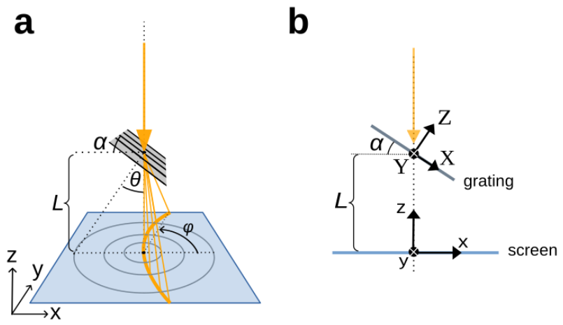
When light is incident on an inclined diffraction grating, i.e., under an angle to the grating normal, it produces diffraction orders on the detector screen that lie on a curved line (cf. Figure 1a), and the curvature increases with increasing inclination [48,49,50]. The opening of the curved line is into the direction where the fibers are closest to the detector screen. At the detector plane, the conical diffraction curves are hyperbolas for inclinations , and ellipses for (see Figure 1b):
where are the coordinates on the detector screen with lying in the center of the screen, and L is the distance between the detector screen and the center of the grating. The coordinate system has been chosen such that the y-axis lies perpendicular to the grating slits, and the negative z-axis in the direction of the incident light (cf. Figure 1a). If the grating slits are parallel to the x-axis, i.e., parallel to the screen (), the diffraction orders lie on a straight line: . If the grating slits are parallel to the z-axis, i.e., perpendicular to the screen (), the light is not diffracted, i.e., . The full derivation can be found in Appendix A, Secs. Appendix A.1-Appendix A.2.
When evaluating the conical diffraction curve for a given inclination angle at a specific polar angle , the points of intersection (peaks) lie an azimuthal distance apart (see Figure 1b). If we know the polar angle and the azimuthal peak distance , we can compute the absolute inclination angle of the grating using the following equation:
Figure 1c shows a plot of the azimuthal peak distance vs. inclination for different polar angles. The full derivation of Eq. (2) can be found in Appendix A, Sec. Appendix A.3.
2.2. 3D-Printed Phantoms
As basis for the 3D-printed phantoms, we used a densely grown fiber bundle to mimic naturally grown fibers in biological tissues. The fiber bundle is similar to the one used in previous simulation studies [40] and was generated with the FastPLI software [51] (https://github.com/3d-pli/fastpli), using fiber diameters of µm. The software starts with a random uniform distribution of points in the yz-plane which are used as starting points for parallel straight fibers along the x-direction. Collisions between overlapping fiber segments are solved by slightly displacing the fiber segments, yielding a naturally grown fiber bundle without collisions. The resulting fiber bundle was rotated by different inclination angles () and cropped to a volume of µm3. Four side walls with 2 µm thickness were added for stabilization. The resulting 3D-models are shown in Appendix C, Figure A2a.
The three-dimensional fiber phantoms were fabricated by two-photon polymerization using a Photonic Professional GT+ system (Nanoscribe GmbH & Co. KG, Germany). Two-photon polymerization enables the direct fabrication of three-dimensional microstructures through localized polymerization of a photosensitive material within the focal volume of a tightly focused femtosecond laser beam. Owing to the nonlinear nature of two-photon absorption, polymerization is confined to the focal volume, enabling the fabrication of three-dimensional structures with sub-micrometer features and large overhanging sections without the need for sacrificial support structures.
The structures were printed on fused silica substrates using IP-Dip2 (Nanoscribe GmbH & Co. KG, Germany, refractive index for room temperature and visible light) in DiLL (Dip-in Laser Lithography) mode using a printing objective. Printing parameters were defined using the Describe slicing software and kept constant for all structures. Both the slicing and hatching distances were set to 0.1 µm, resulting in closely spaced voxel trajectories in both the vertical and lateral directions. These parameters were selected to ensure sufficient polymerization throughout the fiber volume while maintaining the designed microscale geometry and minimizing overpolymerization. The laser power was set to 15 mW, and a scan speed of µm s−1 was used for all structures.
The orientation of the laser scan trajectories relative to the fiber geometry was optimized to facilitate the fabrication of the large unsupported fibers. Specifically, the hatching direction was oriented perpendicular to the longitudinal axis of the fibers, such that individual laser scan trajectories traversed the fiber cross-section rather than extending along the fiber axis. This transverse scanning strategy was employed to improve the structural stability of the fibers during fabrication and reduce the risk of collapse of the unsupported sections.
Following laser exposure, the structures were developed to remove unpolymerized IP-Dip2. Immediately after printing, the substrates were immersed in propylene glycol monomethyl ether acetate (PGMEA) for 25 min, followed by rinsing in isopropyl alcohol (IPA) for 5 min. To minimize capillary forces during drying and thereby reduce the risk of structural collapse, the substrates were subsequently immersed in NOVEC 7100 for 1 min. The substrates were then removed from the solvent and allowed to dry, yielding the final free-standing polymerized fiber structures.
2.3. Biological Samples
For the validation on biological samples, two sections of a vervet monkey brain were used (no. 502 and 504). Appendix C, Figure A3 shows an overview of the samples together with anatomical annotations.
The brain was collected for a different study from a healthy, 2.4-years-old, male vervet monkey. The preparation has been described in previous articles [22,33,34,35,36,40,52]: Following perfusion-fixation with 4% paraformaldehyde, the brain was removed from the skull within 24 hours after death and fixed in 4% paraformaldehyde for several weeks. Subsequently, the brain was cryo-protected in 20% glycerin and 2% dimethyl sulfoxide, deeply frozen, and coronally cut from anterior to posterior into 60 µm-thin sections using a cryostat microtome (Polycut CM 3500, Leica Microsystems). The resulting brain sections were mounted on glass slides, embedded in 20% glycerin solution, and cover-slipped without staining. Two sections from the middle (no. 502 and 504) were selected for analysis. The embedding took place 14 years before the measurements of this study.
The brain was obtained in accordance with the Wake Forest Institutional Animal Care and Use Committee (IACUC #A11-219). Euthanasia procedures conformed to the AVMA Guidelines for the Euthanasia of Animals, using ketamine/pentobarbital anesthesia followed by perfusion with phosphate buffered saline and fixation with 4 % paraformaldehyde. All animal procedures were in accordance with the National Institutes of Health guidelines for the use and care of laboratory animals and in compliance with the ARRIVE guidelines.
2.4. Bright-Field Microscopy Measurements
The bright-field microscopy measurements of the 3D-printed phantoms (Appendix C, Figure A2c) were performed with a Keyence VHX-6000 Digital Microscope, using a VH-ZST dual-objective zoom lens with digital magnification and a high-brightness white LED for illumination.
2.5. ComSLI Measurements
2.5.1. Scatterometry Measurement
The ComSLI scatterometry measurements were performed as described in Menzel et al. (2021b & 2023) [34,36], using the setup shown in Figure 2b, which contains an LED display, a sample stage, and a camera. A light-absorbing conic tube was installed between sample and camera objective to avoid detection of ambient light and suppress internal reflexes. For the validation measurements on (inclined) brain sections, a tiltable specimen stage was employed: The stage was attached to the vertical axis via a rotation mount with degree scale; to allow for in-plane rotations, the sample was attached to the rotation mount via an additional joint.
The LED display (Absen LED AW2.8) contains RGB-LEDs arranged in a grid pattern with 2.87 mm pitch. The optical system consists of a CMOS RGB-camera (Basler acA5472-17uc) and an objective lens (Rodenstock Apo-Rodagon-D120 with 5.6 f-number) positioned 241 mm away from the sample. The camera records images with pixels and a pixel size of approx. 3 µm, yielding a field of view of approx. cm2. The lateral optical resolution is between µm and µm (determined by a USAF target).
The samples were illuminated using a grid of kernels of (white) RGB-LEDs, and an image was taken for every illumination angle. From the resulting image series, scattering patterns were reconstructed for every image pixel (cf. Figure 2b), showing the intensity scattered into the camera for each of the illumination positions at a certain location in the sample.
Measurements were performed with gain 1, average 4, and different exposure times to gain enough signal, but avoid over-exposure: 4 seconds for the 3D-printed phantoms, 3 seconds for the measurements of the vervet corpus callosum and cingulum, and 2 seconds for the measurements of the vervet fornix. Samples were placed at different heights above the LED display yielding different polar illumination angles: The 3D-printed phantoms were placed 150 mm above the LED display, yielding a maximum polar illumination angle in x and y of . Vervet brain section no. 502 (measured under different tilt angles, see Sec. 3.2) was placed at 255 mm above the LED display (). Vervet brain section no. 504 (measured for different regions, see Sec. 3.3) was placed at 235 mm above the LED display (). The brain sections were placed higher than the 3D-printed phantoms because the tiltable specimen stage was used for the measurements. As vervet brain section no. 502 had to be rotated in-plane, it was placed slightly higher than the other section to avoid contact with other setup components. For the 3D-printed phantoms, the conic tube was placed such that the opening is cm above the sample holder. For measurements with the tiltable specimen stage, the conic tube had to be moved up by cm, yielding circular artifacts in the measured scattering patterns. The artifacts were compensated by subtracting the averaged scattering pattern of a region without tissue.
Each scattering pattern has its highest intensity in the center where unscattered light directly reaches the camera. Depending on the position of the image pixel from which the scattering pattern has been generated, the center is at slightly different positions within the -pixel scattering pattern. When plotting a measured scattering pattern, the center is determined as the mid point of the area with the highest intensity, and concentric rings with steps are plotted around the center for reference.
2.5.2. Angular Measurement
The angular ComSLI measurements were performed as described in Abbasi et al. (2026) [25], using the setup shown in Figure 2c: Instead of an LED display, the setup contains a rotating LED spot which was rotated at a fixed polar angle () in steps around the sample. This means that only 24 illuminations were required instead of the 1600 for scatterometry, reducing the acquisition time from hours to minutes.
The resulting image series was reorganized into scattering signals (azimuthal line profiles) for each image pixel, showing the intensity of the normally scattered light recorded by the camera for each of the 24 azimuthal illumination angles at a certain location in the sample.
Images were recorded with a monochrome CMOS camera (BASLER acA5472-17um). Camera lens and distances were the same as for the scatterometry measurements (Rodenstock Apo-Rodagon-D120 with 5.6 f-number, 241 mm sample-camera-lens distance, 5.6 cm sample-cone distance), yielding the same pixel size, field of view, and resolution. As LED spot, a fiber-coupled white-light LED was used (Prizmatix, 400-750 nm range, 443 nm peak wavelength); the light was guided through a 2 m long, multimode fiber with a core diameter of 1500 µm, and passed through a collimator (Prizmatix, FCM1-0.5-CN) and an engineered diffuser (Thorlabs, ED1-S20-MD) for beam shaping.
All measurements were performed with an exposure time of 15 ms, averaging over 4 images, and 130 mm distance between sample and LED spot.
2.6. 3D-sSAXS Measurement
The 3D-scanning small-angle X-ray (3D-sSAXS) measurement (used for validating the determined fiber inclinations in vervet brain section no. 504) has been performed on an adjacent vervet brain section (section no. 511, prepared as described in Sec. Section 2.3) for a different study (Menzel et al. (2023) [36]). For the 3D-sSAXS measurement, the brain section was removed from the glass slides, immersed in phosphate-buffered saline solution for two weeks, placed between two 170 µm-thin cover slips, and sealed. The measurement was performed with a beam of 15 keV photon energy, 100 µm diameter, 0.7 sec exposure time, rotation angles, mm2 field of view, and 100 µm-steps in x and y. The fiber inclination angles were computed by analyzing the scattering patterns at different sample rotation angles as described in Georgiadis et al. (2020) [32]. The fiber inclination angles are shown in Figure 6A in [36], and the dataset [53] is available from Zenodo under a CC BY 4.0 license (https://creativecommons.org/licenses/by/4.0/); histograms were generated for selected regions for comparison.
2.7. Data Analysis
2.7.1. Conical Diffraction Curve Fitting
To estimate the fiber inclination angle from a measured scattering pattern, the conical diffraction curves (Figure 1b) were fitted to the points of highest intensity in the scattering patterns, not taking the unscattered light in the center into account. To identify the points of highest intensity, a peak finding approach was used as illustrated in Appendix C, Figure A4a-b:
Azimuthal line profiles were calculated from a scattering pattern for circles with radii between 5 and 18 pixels in steps of 1 pixel. 5 and 18 pixels are the minimum and maximum possible radius within a px scattering pattern, excluding the unscattered light in the center and taking a maximum center shift of 2 pixels into account. The profiles show the interpolated intensity of the scattering pattern at 64 equidistant azimuthal angles for each radius (see Figure A4a, black dots). The azimuthal profiles were sub-sampled in 1-steps and subsequently smoothed by a Gaussian kernel with a standard deviation of 12 (Figure A4b). In the resulting smoothed profiles, peak positions were determined using the scipy.signal.find_peaks function of the SciPy Python library (version 1.15.3) [54], using a repeated version of the signal to take the periodicity into account. Peaks were ignored if they were less than of the maximum of the signal, or if their prominence was less than of the maximum of the signal. The prominence is defined by the vertical distance between the top of the peak and the higher of the two neighboring minima, and it was determined using the scipy.signal.peak_prominences function. The two peaks with the highest prominence were selected and marked in the scattering pattern as red dots (see Figure A4a).
Finally, a least-squares fit was used to find the theoretical diffraction curve that most closely matches these points of highest intensity, using -steps. Only curves going through the center of the scattering pattern were considered. For the 3D-printed phantoms, an in-plane angle of was assumed. For the biological samples, both and were fitted. To estimate the goodness of the fitted inclination and in-plane angle, the root-mean-square (RMS) distance was computed for all different inclinations and in-plane angles for the fitted - and -values, respectively, and the range of inclinations and in-plane angles for which the RMS distance differs from the minimum was determined.
2.7.2. Fiber Inclination from Peak Distance
The angular ComSLI measurements were analyzed as described in Menzel et al. (2021a) [33], using the Scattered Light Imaging ToolboX (SLIX), version 2.4.2 (https://github.com/3d-pli/SLIX) [55]. Apart from an in-plane fiber orientation map, SLIX computes the azimuthal peak distance (distance between two prominent peaks in the azimuthal line profile) for every image pixel. Peaks with a prominence above 8 % of the total signal amplitude (max−min) were considered as prominent peaks. Pixels with one peak have zero peak distance and pixels with more than two peaks were not evaluated.
3. Results
We first analyzed the scattering patterns of samples with known fiber orientations. For this purpose, we performed ComSLI scatterometry measurements on the 3D-printed phantoms with different fiber inclinations, and fitted the conical diffraction curves to the measured scattering patterns (Sec. Section 3.1). Subsequently, we compared our results to measurements of biological fibers (nerve fibers in the vervet brain sections). To study nerve fibers with different inclination angles, we selected a region with mostly in-plane parallel fibers, tilted the brain section by different angles, and analyzed the resulting scattering patterns (Sec. Section 3.2). Finally, we measured different regions in a vervet brain section with ComSLI scatterometry and estimated the fiber inclinations from the measured scattering patterns (Sec. Section 3.3). To investigate the potential of speeding up the measurement, we performed an angular ComSLI measurement on the same brain section, estimated the local fiber inclinations from the azimuthal peak distances, and compared our results to the fiber inclinations obtained from a 3D-sSAXS measurement of an adjacent section.
3.1. 3D-Printed Phantoms
To verify that the 3D-printed phantoms resemble the original 3D-models of which we know the fiber geometries/inclinations, we measured all 3D-printed phantoms with a bright-field microscope (Appendix C, Figure A2c). Comparing these images to the original 3D-models (Figure A2a-b) shows that a few fibers are missing for intermediate inclination angles (marked by red ellipses), but the positions and shapes of all printed fibers correspond to what we would expect from the original 3D-model. Therefore, we can assume that the printed fibers are oriented as defined by the 3D-models, i.e., all fibers have an average in-plane azimuthal angle of (along the x-axis) and an average out-of-plane inclination angle of .
Figure 3 shows the results of the ComSLI scatterometry measurement for the differently inclined 3D-printed fiber bundles, and the comparison with the conical diffraction model. To obtain a representative scattering pattern for each 3D-printed phantom, the scattering patterns obtained from the inner image pixels of each sample were averaged. Figure 3a-c shows the 3D-model, top-view, and microscopy image exemplary for the 40-inclined phantom; the red square in (c) indicates the region in which the scattering patterns were evaluated.
The resulting averaged scattering patterns are displayed in Figure 3d. They show a high-intensity line going through the center; its curvature increases with increasing inclination and the opening is towards the right, i.e., where the fibers are closest to the LED-display. The middle high-intensity lines closely match the theoretical conical diffraction lines that were computed for the respective inclination angles (magenta dashed lines in Figure 3e). Side lines are visible for 0, 20 and 40 (indicated by white dotted lines in (e)); the curvature increases with the inclination, while right side lines appear more curved than left side lines.
To check whether the theoretical curves accurately describe the measurement data and to investigate how reliable we can estimate the fiber inclination from a measured scattering pattern, we fitted the conical diffraction model to the measured scattering patterns (Figure 3f). The red dots show the highest-intensity points determined from the peak finding approach, and the black dashed lines show the curves obtained from the least-squares fit as described in Sec. Section 2.7.1. Figure 3g shows a direct comparison of the fitted curves (black) and theoretical curves (magenta), demonstrating that the fitted curves closely match the theoretical diffraction curves, especially for .
In Figure 3h, we see the inclination angles of the 3D-printed fibers that were used to compute the theoretical diffraction curves plotted against the inclination angles estimated from the fitting (red dots). The estimated inclination angles lie close to the theoretical expectation (diagonal dashed line); the maximum deviation is for the in-plane fiber bundle. The graph in Figure 3i shows the normalized RMS distance between the highest-intensity points and the fitted line for different (fitted) inclination angles. To indicate the precision of our fit, the dotted vertical lines mark the ranges for which the RMS distance differs less than 1 % from the minimum; these ranges are also indicated in (h). The exact values (fitted inclination angles, 1% RSM distance intervals, minimum RMS distance and standard deviation) are listed in Appendix B, Table A1.
For , the inclination angles estimated from the fitting correspond to the actual fiber inclination angles of the 3D-models within the 1% RMS distance ranges. For , the estimated inclination is slightly over-estimated, even when taking this range into account.
As can be seen in Figure 3i, the RMS distance vs. fitted inclination curve has a broader minimum and thus a lower precision for smaller inclination angles than for larger inclination angles. This is due to the fact that the theoretical diffraction curves for smaller inclination angles lie closer together than for larger inclination angles (cf. also Figure 1b). Even if the highest-intensity points lie almost perfectly on a conical diffraction curve for a certain , another diffraction curve with a slightly smaller or larger describes these points almost equally well so that a slight change in the points’ locations already leads to a different fitted inclination: while the theoretical/fitted curves in Figure 3g look almost identical for , the estimated inclination differs by from the theoretical value. For larger inclination angles, the fitting is much more stable: while the theoretical/fitted curves in Figure 3g look clearly different for , the estimated inclination only differs by from the theoretical value.
However, larger inclination angles have another problem: Instead of a clearly defined high-intensity line/hyperbola, the highest intensity is expected along an ellipse, leading to an accumulation of intensity and making it more difficult to accurately determine the points of highest intensity. As can be seen in Figure 3f, only four points of highest intensity were found for while the right part of the high-intensity region does not yield clearly defined intensity peaks. This leads to a wrong fitting and thus an over-estimation of the actual inclination angle. Although the 1% RMS distance intervals are very small for large inclinations, the fitted inclination is therefore likely to be inaccurate.
Despite these challenges, all fitted inclination angles were found to be mostly accurate up to , showing that the conical diffraction model accurately describes the measurement data and can be used to estimate the underlying fiber inclination.
3.2. Tilted Vervet Brain Section
So far, we have only considered artificial fibers. To find out whether the conical diffraction model can be used to estimate the inclination angles of biological fibers, we investigated differently inclined nerve fiber bundles in a vervet monkey brain section. Adjacent sections from the same vervet brain have already been used in multiple studies [22,33,34,35,36,40,52] to investigate nerve fiber orientations with scattered light imaging.
To study nerve fiber bundles with different inclination angles, we selected a region with mostly in-plane, horizontal fibers (corpus callosum in a coronal brain section) and tilted the section by different tilt angles to mimic different fiber inclinations. Figure 4 shows the results of the ComSLI scatterometry measurements and the comparison to the conical diffraction model for different tilt angles.
Vervet brain section no. 502 (Figure 4a) was selected for the analysis. The section was rotated in the xy-plane to align the fibers in the corpus callosum with the horizontal x-axis, and tilted around the y-axis by different angles to mimic different out-of-plane fiber inclinations (see Figure 4b). The horizontal alignment was required to ensure that the in-plane orientations of the fibers do not change much during the tilting and that the out-of-plane angles increase mostly linearly with the tilt angle. For evaluation, we selected a -pixel region that lies on the tilt axis (indicated by the red dots in Figure 4b) to ensure that the evaluated regions lies in focus for all tilt angles. The section was tilted by to achieve similar fiber inclinations as the ones in the 3D-printed phantoms; larger tilt angles were not possible as the tiltable specimen stage gets too close to the LED display and hinders the measurement. As mentioned in Sec. Section 2.5.1, the conic tube had to be moved up for the tilting, leading to circular artifacts in the averaged scattering patterns (Figure 4c, magenta arrows). To remove the circular artifacts, the original scattering patterns were calibrated by subtracting the averaged scattering pattern of a region without tissue for the respective tilt angle (Figure 4d).
Figure 4e shows the highest-intensity points of the calibrated scattering patterns (red dots) determined by the peak finding approach together with the fitted conical diffraction curves (black dashed lines). In contrast to the 3D-printed phantoms for which the underlying fiber orientations and thus the theoretically expected diffraction curves are known, the nerve fiber orientations in the measured region are not exactly known. Although we selected a region in the corpus callosum which is known to contain mostly parallel in-plane fibers in a coronal brain section [56,57], the fibers could still have a small out-of-plane inclination angle which can be positive/clockwise or negative/counter-clockwise. Also the in-plane fiber angle can slightly differ from zero as the microscopic fiber orientations are not visible and the fiber bundle can only be roughly aligned with the x-axis of the specimen stage. To still investigate whether the fitted fiber orientations are self-consistent taking the respective tilt angles into account, we fitted both fiber inclination and in-plane angle for each tilt angle, rotated the fitted fiber orientation () back to the orientation before the tilt, and took the average over all tilt angles as theoretical expectation for zero-tilt fibers: . Figure 4f shows the fitted curves (black) in comparison to the theoretical curves (magenta). Figure 4g,h show the theoretical inclination and normalized RMS distance plotted against the fitted inclination together with the respective 1% RMS distance intervals. The exact values (fitted and theoretical inclination/in-plane angles, back-rotated values, 1% RMSD intervals, minimum RMS distance and standard deviation) can be found in Appendix B, Table A2 and Table A3.
As can be seen, the fitted curves closely match the theoretically expected diffraction curves, and the fitted inclination values correspond to the theoretical inclination values within their 1% RMS distance intervals. The difference between fitted and theoretical inclination angles lies between for and for . The difference between fitted and theoretical in-plane angles lies between for and for .
This shows that the conical diffraction model also accurately describes the scattering on biological fibers such as nerve fibers, at least until an inclination angle of about 60. Larger inclination angles could not be validated with the employed tiltable specimen stage.
3.3. Different Vervet Brain Regions
Next, we estimated the fiber inclinations for different brain regions from the measured scattering patterns (scatterometry ComSLI) as well as from the azimuthal line profiles (angular ComSLI). The results are shown in Figure 5.
Scattering patterns were obtained for four different regions in vervet brain section no. 504 (Figure 5a): 1–corpus callosum (cc), 2–fornix (fx), 3–bottom cingulum (cg, bottom), and 4–top cingulum (cg, top). Figure 5c shows the (averaged) scattering patterns of these regions together with the fitted conical diffraction curves (black dashed lines). The corpus callosum and fornix were averaged over patterns, while the bottom cingulum was averaged over patterns as this was the largest homogeneous region that could be found in this area. The top cingulum was averaged over patterns to average out speckle that was observed in these patterns. The fitted inclination and in-plane angles () are indicated below the patterns. The graphs at the bottom show the azimuthal line profiles evaluated at 20 polar angle (red circles in the scattering patterns).
As expected, the corpus callosum contains mostly in-plane fibers () and the azimuthal line profile shows two clear peaks that lie almost 180 apart. The fornix () and especially the cingulum () contain more out-of-plane fibers; the azimuthal peak distances are smaller than for the corpus callosum. The top part of the cingulum (region 4) yields a mostly isotropic scattering pattern with no high-intensity line and an almost flat azimuthal line profile, indicating a highly inclined fiber bundle. Comparing this scattering pattern to the one obtained from a 3D-nanoprinted phantom with (Figure 5b) shows that this region contains probably nearly vertical fibers.
Measuring the -pixel scattering patterns with a ComSLI scatterometry measurement (requiring 1600 images) and computing the fitted inclination angles from each scattering pattern is very time consuming. To investigate whether we can speed up the measurement and estimate the inclination angles of all image pixels in a larger field of view, an angular ComSLI measurement was performed on the same brain section, in the region containing corpus callosum, fornix, and cingulum (yellow rectangle in Figure 5a) using a polar illumination angle of (see Sec. Section 2.5.2). The inclination angles were computed from the azimuthal peak distances as described in Sec. Section 2.7.2. The resulting inclination map is shown in Figure 5d and histograms of the four regions from which the scattering patterns were computed are shown in Figure 5f (with the fitted inclination angles indicated by colored vertical lines).
To validate the fiber inclinations obtained for vervet brain section no. 504, we compared the inclinations to those obtained from a 3D-sSAXS measurement of an adjacent section (see Sec. Section 2.6) that was measured for a previous study [53] (section no. 511, shown in Figure 6A in [36]). 3D-sSAXS has been shown to reliably determine the 3D-orientations of nerve fibers in brain tissue [32]. Figure 5e shows the inclination map from the 3D-sSAXS measurement and Figure 5g shows the histograms for the marked regions (similar regions as the ones from which the scattering patterns were computed).
When comparing the angular ComSLI and 3D-sSAXS measurements, one should note that the brain sections are not directly adjacent but lie 420 µm apart. Furthermore, the inclination angles were not computed for all image pixels in the angular ComSLI measurement as some azimuthal profiles did not yield one or two prominent peaks (shown as black pixels in Figure 5d), which makes the inclination map look darker in some places than the one from 3D-sSAXS. Also, the angular ComSLI measurement was performed with a polar illumination angle of for better comparison with previous studies [25,27]. However, this implies that inclination angles larger than 68 could not be resolved (), as shown in Appendix C, Figure A4f. These pixels are displayed yellow in (d), while they are displayed with different ranges of yellow in (e).
Despite these differences, the histograms in Figure 5f-g show similar tendencies regarding the fiber inclinations in the investigated regions: The histograms of corpus callosum and fornix show similar value distributions, while the bottom cingulum yields a broader distribution for the 3D-sSAXS measurement than for the angular ComSLI measurement. The top cingulum features high fiber inclinations in both measurements while the angular ComSLI measurement is clipped at 68 inclination. Comparing the results to the fitted inclinations obtained from the measured scattering patterns (colored vertical lines in the histograms), the fitted inclinations of corpus callosum and cingulum are compatible with the fiber inclinations in the histograms, while the inclinations in the fornix seem to be actually smaller than the fitted inclination obtained from the scattering pattern. However, it should be noted that the scattering patterns were measured up to a polar angle of 26, while the angular ComSLI measurement was performed with a polar illumination angle of 44, which naturally leads to differences. Another observation we can make when comparing the measured scattering patterns to the out-of-plane fiber orientations obtained from the 3D-sSAXS measurement is that the out-of-plane directions of the fibers determined by the 3D-sSAXS measurement (indicated by 3D-arrows in (e)) correspond to what we expect from the opening of the curvatures observed in the measured scattering patterns in (c): the opening of the curvature is in the direction in which the fibers lie closest to the LED-display, i.e., the image plane.
The results show that the fiber inclinations estimated from the measured scattering patterns for different brain regions seem plausible. Using angular ComSLI and estimating the fiber inclination from the azimuthal peak distance seems to give a first good guess of the out-of-plane fiber orientations, but is limited especially when it comes to larger fiber inclinations.
4. Discussion
Although previous simulations and experimental studies [34,36,40] suggest that inclined (nerve) fibers lead to a curved high-intensity line in ComSLI scattering patterns, a quantitative description with an analytical model has not been realized so far. Recent advances in two-photon polymerization (2PP) allowed us to 3D-nanoprint fiber bundles that mimic biological fibers (micrometer diameters, µm inter-fiber gaps) with known underlying geometry. In this way, we were able to study how the scattering behavior depends on the fiber inclination while leaving all other parameters unchanged.
Compared to other light-based 3D fabrication approaches, such as digital-light processing [58] which is limited to several microns resolution, the sub-micrometric feature resolution of 2PP [46] is less affected by potential over-polymerization issues which would affect the quality of few microns diameters fibers and related inter-fiber gaps. 2PP recently enabled 3D-printing of nanopillar arrays with 500 nm diameter for neuromechanobiology studies [46]. Future advancements might include the use of biomaterials whose mechanical properties are closer to nerve fibers, such as photocrosslinkable hydrogels [59,60].
The 3D-printed fiber bundles used in this study are similar to those used in previous FDTD simulations [40]: the fibers are uniformly randomly distributed, have slightly different fiber diameters, and are naturally “grown”, i.e., not completely straight (cf. Appendix C, Figure A2). Although dimensions and growth patterns were chosen to mimic biological fibers as closely as possible, the 3D-printed phantoms differ from real biological fiber tissue and from the model used in the FDTD simulations [40]: First of all, to ensure stability during 3D-printing, the fibers were printed from a single solid material (IP-Dip2, ) in air (), leading to higher refractive index differences than in biological fiber tissues, where the fibers usually have a lower refractive index [61,62] and are surrounded by an aqueous solution or other materials with higher refractive indices than air. In addition, not all biological fibers can be modeled as solid fibers with a single refractive index: Nerve fibers (myelinated axons) consist of an inner axon core with lower refractive index than the outer myelin sheath. In the FDTD simulations, nerve fibers were modeled as inner axon (), outer myelin sheaths (), and surrounding glycerin/embedding solution (). Second, the diameters of the printed fibers were µm. Most nerve fibers in the investigated brain regions, like the corpus callosum, are expected to have diameters of 1 µm or less [42,43,44], while some nerve fibers can also have diameters of several microns. The FDTD simulations were therefore performed with µm fiber diameters, which is closer to the illumination wavelength. Another difference is that the FDTD simulations were performed with coherent light, while the ComSLI measurements were performed with mostly incoherent LED light. However, coherent Fourier scatterometry measurements already showed that the scattering patterns of a vervet brain section are expected to look similar to ComSLI scattering patterns when being measured with coherent (laser) light [63]. And previous studies also support an effectively incoherent description of the intensities detected in a ComSLI measurement [64].
Although the 3D-printed fibers can mimic biological fibers only to a certain extent, the measured scattering patterns of the 3D-printed phantoms and of the tilted corpus callosum showed a similar behavior for inclined fibers: While the nerve fiber bundles seem to scatter the light more broadly (Figure 4d vs. Figure 3d), the points of highest intensity (red dots) lie on the same line as predicted by the conical diffraction model for (Figure 3f,g and Figure 4e,f). This shows that the 3D-printed phantoms can be used for modeling the scattering behavior on biological fibers. It should be noted that tilting the corpus callosum section is different from measuring a horizontal brain section with inclined fibers which are cut off at the bottom and top (as in the vervet brain section investigated in Figure 5). However, the comparison with the 3D-printed phantoms in which the fibers are also cut off shows that similar scattering patterns are expected for all investigated inclinations.
One difference between the scattering patterns of biological samples and 3D-printed phantoms are the side lines that are visible for the 3D-printed phantoms (Figure 3e, white dashed lines). The side lines are probably caused by the fact that – for smaller inclination angles – multiple fiber layers are located on top of each other, i.e., in addition to the (in-plane) periodicity of a grating, there is also an in-depth periodicity in the z-direction causing higher orders. The reason why these higher orders are not visible for the vervet brain sections could be that the nerve fiber tissue has less periodicity and a lower refractive index difference than the 3D-printed phantoms.
The fiber inclinations estimated from the measured scattering patterns are very close to the theoretical expectation, both for the 3D-printed phantoms and the tilted corpus callosum. The differences between fitted and expected inclination values are 3° or less (Appendix B, Tabs. Table A1 and Table A2); the differences between fitted and expected in-plane angles are 0.8° or less for the tilted corpus callosum (Appendix B, Tabs. Table A3). We should note that the theoretical expectation for the tilted corpus callosum was based on an estimate (average) of fitted values, but we show that the model is self-consistent as the tilt angles of the measurements are known.
Our study shows that the highest-intensity points observed in the measured scattering patterns of inclined (nerve) fibers lie on conical diffraction curves up to 60° inclination (Figure 4). While we were able to show that the conical diffraction model still applies to higher inclination angles for 3D-printed fibers, we could not validate this behavior for biological fibers. For the validation, we tilted a mostly in-plane fiber bundle (corpus callosum in coronal vervet brain section) so that the maximum possible inclination angle was limited by the maximum tilt angle of the specimen stage. For tilt angles , the specimen stage would block the incident light from the LED-display. The reason why we selected a mostly in-plane fiber bundle as starting point is that it allowed us to visually determine the in-plane fiber orientation and to properly align the fiber bundle with the x-axis to achieve the maximum possible fiber inclination.
Because of the limited tilt angle, we cannot confirm whether highly inclined nerve fibers () show a similar scattering behavior as the 3D-printed fibers, for which the high-intensity points of the scattering pattern lie on an out-of-center ellipse in agreement with the conical diffraction model, or whether they show a broader scattering pattern for and 80° as predicted by the FDTD simulations [40]. However, we do observe a mostly isotropic scattering pattern for highly inclined nerve fibers as in the upper cingulum of the coronal vervet brain section, where the 3D-sSAXS measurement of an adjacent section yielded inclination angles of 80° and higher (Figure 5e). Both the measured scattering patterns of the 3D-printed phantoms and the simulated scattering patterns of the FDTD simulations yield an isotropic scattering pattern with broad scattering around the center (cf. Figure 5b) for a nearly vertical fiber bundle.
We here present an automated way to estimate fiber inclinations from measured scattering patterns. However, not only is the measurement (acquiring images) very time consuming, the data analysis also takes a lot of time due to the large amount of data. We therefore studied the potential of using angular ComSLI (requiring only 24 instead of 1600 images) to estimate the inclination from the azimuthal peak distance in the scattering profile of each image pixel, instead of analyzing full scattering patterns (see Figure 5d,f).
However, when estimating the inclination from the azimuthal peak distance, there is a theoretical limit given by the conical diffraction model (see Figure 1c and Appendix C, Figure A4f). The maximum inclination angle that can be determined is: (see Eq. (A19) in Appendix A). This means that the larger the illumination angle , the smaller the maximum inclination that can be determined. For higher inclinations, diffraction occurs along an ellipse that is not intersected anymore by larger polar angles (see Figure 1b and Figure A4c). When looking at the relationship between azimuthal peak distance and inclination angle as predicted by the conical diffraction model (Figure 1c), we also see that the slope of this curve depends on the polar illumination angle. Ideally, the curve should be as steep as possible, so that the uncertainty in the peak distance, which is difficult to determine exactly, does not lead to large changes in the estimated inclination. However, this can only be obtained by a larger polar illumination angle, which leads to a lower . The polar illumination angle of 44°, which is currently used for angular ComSLI measurements, is a good compromise (see dashed curve in Figure 1c): It allows a relatively good estimation of the inclination up to 60°. To better determine higher inclination angles, an additional measurement should be performed with a smaller polar illumination angle, e.g., which allows to determine inclinations up to 85° (blue curve in Figure 1c). Note that there is also a practical limit regarding the minimum polar illumination angle, namely when the (unscattered) light directly shines into the camera.
To realize measurements with multiple polar angles, LED rings of different sizes could be used. To reduce measurement time, Hadamard illumination [64] could be applied to each angular measurement allowing to reduce exposure time by multiplexing multiple illumination directions at once. Another possibility to speed up the measurement could be to make use of compressed sensing; this might even allow to measure scattering patterns with lower resolution [65] but sufficient detail for conical diffraction curve fitting. However, even when measuring at multiple polar angles or full scattering patterns, it will still be difficult to accurately estimate the inclination for higher inclined fibers, as light is expected to scatter more broadly, i.e., not along a defined line, and peak locations become more difficult to determine. To determine the best illumination strategy and the best compromise between measurement time (number of images/illumination angles) and accuracy of estimated inclination angles will be subject of future studies.
The measured scattering patterns shown in this study are the average of multiple image pixels ( pixels or more, corresponding to an area of µm2 or more). The averaging was done to study the overall behavior of inclined fibers and not to depend on local or statistical fluctuations. As the scattered light is mostly incoherent, the analytical model describing the behavior of the averaged scattering patterns is also valid assuming a smoothly varying geometry due to homogeneous tissue regions. The angular ComSLI measurement shown in Figure 5d shows the estimated inclination angles per image pixel and is thus more prone to noise. While the conical diffraction curves can be fitted to multiple highest-intensity points in a measured scattering pattern, the angular ComSLI measurement yields a 1D scattering signal per image pixel and the inclination is computed from the azimuthal peak distance in this line profile. As can be seen in Figure 5d, multiple image pixels could not be evaluated (shown in black) due to noisy signals with more than 1–2 prominent peaks. Moreover, SLIX uses a simple peak-finding algorithm in which discretization is accounted for by computing the geometric center of the peak tip [55] so that the determined peak distances might not be completely accurate. More advanced algorithms, e.g., using smoothing and Gaussian fitting, could be employed to determine the peak distance more accurately, however, they will also increase the computing time and might not be feasible for larger fields of view.
Our study is a first proof of concept, showing that the high-intensity points of a measured scattering pattern for inclined biological fibers lie on the same curves as the diffraction peaks of an inclined grating. We here provide for the first time of our knowledge an analytical model (conical diffraction model) allowing to determine the fiber inclination from a measured scattering pattern, or possibly from a measured scattering signal. We show that the model accurately describes our measurement data up to 60° inclination. We used the model to determine theoretical limitations, like the cut-off angle for angular ComSLI, and to determine the best possible inclination estimate for real biological fibers under ideal conditions. We still need to evaluate our inclination estimation in practice, i.e., when performing a pixel-wise evaluation and when speeding up the measurement with angular ComSLI. Future studies need to be performed to investigate how accurate fiber inclinations can be estimated per image pixel in a reasonable amount of time, and how accurate we can determine the inclination angles of highly inclined fibers.
However, even if only a rough estimate of the fiber inclination angle is possible, it allows us to go from solely 2D-fiber orientations to 3D-orientations, and the estimate can be used, e.g., in fiber tractography algorithms to better follow the course of fibers across adjacent sections, and to better assess the (3D) collagen fiber orientation relative to tumor boundaries. It should be noted that this study only investigated regions with mostly parallel inclined fibers; regions with crossing inclined fibers are expected to show a more complex scattering behavior as the scattering patterns of different 3D-fiber orientations overlay (cf. Figure F3 in [33]). A reliable reconstruction of multiple 3D-fiber orientations per image pixel is therefore much more challenging and requires further research.
In this study, we have only validated our results on brain sections (nerve fibers). However, the nerve fibers showed a similar scattering behavior as the 3D-printed fibers, which have larger diameters and not an inner core with different refractive index. This suggests that our findings can be generalized to muscle fibers, which also have no inner core and larger diameters, and possibly to other types of fibers like collagen.
5. Conclusions
ComSLI is a versatile technique for mapping biological fibers in histological tissue sections: it allows microscopic fiber mapping across large fields of view also in crossing regions, is easy to implement, fast when using angular ComSLI, and compatible with various sample preparations and staining. However, an accurate determination of fiber orientations was so far only possible for in-plane (2D) orientations. Here, we present for the first time of our knowledge an analytical (conical diffraction) model that can be used to determine the out-of-plane fiber inclinations from ComSLI measurements. Using 3D-nanoprinted phantoms with different fiber inclinations, we showed that the highest-intensity points of ComSLI scattering patterns lie along the same curved lines as the diffraction orders of inclined gratings, and that the underlying fiber inclinations can be reconstructed with an accuracy of 3° or higher by fitting conical diffraction curves to these highest-intensity points. We validated our results on biological samples (tilted nerve fiber bundle) up to 60° inclination, and showed that the conical diffraction model can be used to estimate fiber inclinations in a vervet monkey brain section. It is expected that our findings can be generalized to other types of fibers, like collagen or muscle fibers. While the fiber inclinations were determined with high accuracy from scattering patterns obtained with ComSLI scatterometry, we also demonstrated the potential of using the much faster angular ComSLI for estimating fiber inclinations from azimuthal peak distances. In comparison to scatterometry, the determined fiber inclinations turned out to be more error-prone and there is a cut-off for high inclination angles. Further studies are needed to find the best compromise between the number of illumination angles and the measurement time, and to better quantify the behavior of highly inclined () and crossing inclined fibers.
With the provided analytical model, we are finally able to extend ComSLI from 2D-fiber mapping to 3D-fiber mapping. This will open up other applications like facilitating fiber tractography across 3D-volumes (adjacent sections) or allowing a more accurate determination of collagen fiber angles relative to tumor boundaries.
Author Contributions
Conceptualization, M.M. and A.A.; methodology, M.V. and P.v.A.; software, M.V.; validation, M.V.; formal analysis, M.V. and D.S.; investigation, M.V.; resources, M.M. and A.A.; writing—original draft preparation, M.V. and M.M.; writing—review and editing, P.v.A., D.S. and A.A.; visualization, M.V. and M.M.; supervision, M.M and A.A.; project administration, M.M.; funding acquisition, M.M and A.A. All authors have read and agreed to the published version of the manuscript.
Funding
This research was funded by the Delft Bioengineering Institute, the Netherlands (project: Disentangling the Brain’s Fiber Network using 3D-Nanofabrication and Scattered Light), by AIDAS–AI, Data Analytics and Scalable Simulation– which is a Joint Virtual Laboratory gathering the Forschungszentrum Jülich (FZJ) and the French Alternative Energies and Atomic Energy Commission (CEA), and by the National Institutes of Health grant no. R01MH092311 and 5P40OD010965.
Institutional Review Board Statement
The animal study protocol was approved by the Wake Forest Institutional Animal Care and Use Committee (IACUC #A11-219). Euthanasia procedures conformed to the AVMA Guidelines for the Euthanasia of Animals. All animal procedures were in accordance with the National Institutes of Health guidelines for the use and care of laboratory animals and in compliance with the ARRIVE guidelines.
Data Availability Statement
The original data presented in the study are openly available in Zenodo at https://doi.org/10.5281/zenodo.22643344.
Acknowledgments
The authors thank Roger Woods from the UCLA Brain Research Institute for providing the vervet brain sample, the laboratory team at Forschungszentrum Jülich GmbH (INM-1), Germany, for preparing the vervet brain sections, and Bernd Rieger, Delft University of Technology, the Netherlands, for helpful discussions.
Conflicts of Interest
The authors declare no conflicts of interest. The funders had no role in the design of the study; in the collection, analyses, or interpretation of data; in the writing of the manuscript; or in the decision to publish the results.
Abbreviations
The following abbreviations are used in this manuscript:
| CMOS | complementary metal-oxide-semiconductor |
| ComSLI | computational scattered light imaging |
| dMRI | diffusion magnetic resonance imaging |
| FDTD | finite-difference time-domain |
| FFPE | formalin-fixed paraffin-embedded |
| LED | light emitting diode |
| pSHG | polarimetric second harmonic generation |
| (PS-)OCT | (polarization-sensitive) optical coherence tomography |
| RGB | red, green, blue |
| RMSD | root-mean-square distance |
| SLIX | scattered light imaging toolbox |
| 2D/3D | two-/three-dimensional |
| 2PP | two-photon polymerization |
| 3D-PLI | three-dimensional polarized light imaging |
| 3D-sSAXS | 3D-scanning small-angle X-ray scattering |
Appendix A. Derivation of Formulas
In the following, we derive the formulas used to describe the diffraction at an inclined 2D-grating (main Figure 1b) and the corresponding azimuthal peak distances (main Figure 1c).
For the derivation, we assume the setting shown in main Figure 1a (or Figure A1a): The coordinate system is defined such that the x- and y-axes span the detector screen, and the z-axis points from the screen towards the grating. The origin lies in the center of the screen. The grating is oriented such that the y-axis lies perpendicular to the slits, and the x-axis parallel to the projection of the slits onto the screen. The grating is rotated (inclined) around the y-axis by an angle following the right-hand rule. Light falls onto the grating from above, along the z-axis. A point on the screen can be described by as well as by spherical coordinates (polar angle) and (azimuthal angle) defined relative to the center of the grating (where the light hits the grating). We here only consider the case in which the grating slits (or their projection) are oriented along the x-axis. If the grating is rotated around the z-axis by an angle , the diffraction pattern is rotated accordingly.
In addition to the coordinate system of the screen , we define the local coordinate system of the grating (see Figure A1b). In this coordinate system, the X-axis points in the direction of the grating slits, the Y-axis perpendicular to the slits (i.e. in the same direction as the y-axis), and the Z-axis along the grating normal. The origin of this coordinate system lies in the center of the grating, at a distance above the screen.
Figure A1.
Definition of coordinate systems. (a) Schematic showing the diffraction at a grating with inclination angle (main Figure 1a). (b) Local coordinate system () of the grating and coordinate system () of the screen. The X-axis points along the grating slits, the Y-axis perpendicular to the grating slits (in the same direction as the y-axis), and the Z-axis along the grating normal. The coordinate systems are rotated by an angle with respect to each other, and their origins lie at a distance L apart.
Figure A1.
Definition of coordinate systems. (a) Schematic showing the diffraction at a grating with inclination angle (main Figure 1a). (b) Local coordinate system () of the grating and coordinate system () of the screen. The X-axis points along the grating slits, the Y-axis perpendicular to the grating slits (in the same direction as the y-axis), and the Z-axis along the grating normal. The coordinate systems are rotated by an angle with respect to each other, and their origins lie at a distance L apart.
Appendix A.1. Conical Diffraction at an Inclined Grating
Harvey & Pfisterer (2019) [49] provide a grating equation that describes diffraction on a grating in the case that the light strikes the grating at a large oblique angle (conical diffraction). Using their Eqs. (4) and (5) and writing:
we obtain the following equation for :
using . This equation describes a cone in the local coordinate system of the grating , i.e, the cone axis is aligned with the slits of the grating (the X-direction).
Appendix A.2. Intersection with the Detector Plane
In order to describe the conical diffraction curves observed on the screen, we need to transform the coordinates to get from the local coordinate system of the grating to the coordinate system of the screen . The grating coordinate system is related to the screen coordinate system by rotating it around the y-axis by an angle and moving the origin up to ; the y-axis remains unchanged:
Inserting this into Eq. (A1) and using the following trigonometric identities:
we obtain the following equation, which describes the conical diffraction curves observed on the screen at distance L from the grating (see Figure 1b):
Note that in the ComSLI setup, the distance L corresponds to the distance between the LED display and the sample.
The behavior for and follows from taking the limit of equation A9. Taking the limit, we obtain:
The diffraction orders lie on a straight (vertical) line as expected for a non-inclined grating. For the limit, we obtain:
The light is not diffracted and we observe a single bright dot at the origin of the screen.
Appendix A.3. Azimuthal Peak Distance
Relative to the origin/center of the grating (where the light hits the grating), a point on the detector screen can be described by the polar angle and the in-plane azimuthal angle (cf. main Figure 1a):
With this, the above Eq. (A9) can be written in terms of spherical coordinates. After dividing by and by (considering only cases in which ), we obtain:
where we used: , and .
This is a quadratic equation in the form . The solution is given by: . Hence, we obtain (for and assuming ):
Writing and , we can further simplify:
Solving this for yields:
Considering the situation depicted in main Figure 1b, where the grating slits (or their projection) are aligned with the x-axis, we only need to consider the upper part of the curves and the azimuthal peak distance is given by: .
Inserting this into the above equation, we see that the azimuthal peak distance at a given polar angle can be used to estimate the (absolute) inclination angle of the grating (see Figure 1c):
From this equation, the maximum resolvable inclination angle can be obtained by considering the limiting case , in which the two scattering peaks merge. In this case, , yielding:
using the trigonometric identity . Applying the half-angle identities and , this becomes:
Finally, using and noting that , we obtain the closed-form expression:
Appendix B. Fit Values
The tables below list the fit values obtained from fitting the conical diffraction curves to the measured scattering patterns in main Figure 3, Figure 4 and Figure 5:
| fitted in-plane/inclination angles | |
| Min/Max | ranges for which the root-mean-square (RMS) distance differs from the minimum (a measure of the precision of our fit) |
| Min RMSD | minimum RMS distance |
| Stddev RMSD | standard deviation of the RMS distance values |
| theoretical in-plane/inclination angles of the tilted vervet-cc sample, computed under the assumption that the zero-tilt fiber orientation corresponds to the average of the fitted in-plane/inclination angles back-rotated to their orientation before the tilt | |
| fitted in-plane/inclination angles of the tilted vervet-cc sample, back-rotated to their orientation before the tilt |

Table A1.
Fit values for the 3D-printed phantoms for different fiber inclinations (main Figure 3).
Table A1.
Fit values for the 3D-printed phantoms for different fiber inclinations (main Figure 3).
| Min | Max | Min RMSD | Stddev RMSD | ||
|---|---|---|---|---|---|
| 0 | 3.1 | -2.7 | 8.7 | 0.35 | 0.17 |
| 20 | 18.5 | 12.8 | 23.9 | 0.42 | 0.28 |
| 40 | 41.0 | 37.8 | 44.0 | 0.31 | 0.16 |
| 60 | 61.1 | 59.4 | 62.7 | 0.66 | 0.32 |
| 80 | 82.6 | 82.3 | 82.9 | 0.69 | 0.43 |
Table A2.
Fit values for the tilted vervet-cc inclinations for different tilt angles (main Figure 4).
Table A2.
Fit values for the tilted vervet-cc inclinations for different tilt angles (main Figure 4).
| Min | Max | Min RMSD | Stddev RMSD | |||
|---|---|---|---|---|---|---|
| 0 | -4.29 | -6.3 | -14.2 | 0.9 | 0.15 | 0.08 |
| 20 | 15.68 | 14.0 | 6.9 | 20.6 | 0.11 | 0.06 |
| 40 | 35.65 | 38.6 | 34.6 | 42.1 | 0.12 | 0.07 |
| 60 | 55.59 | 56.3 | 54.2 | 58.2 | 0.14 | 0.09 |
Table A3.
Fit values for the tilted vervet-cc in-plane orientations and the back-rotated values for different tilt angles (main Figure 4).
Table A3.
Fit values for the tilted vervet-cc in-plane orientations and the back-rotated values for different tilt angles (main Figure 4).
| Min | Max | |||||
|---|---|---|---|---|---|---|
| 0 | 2.98 | 2.8 | 1.8 | 3.8 | 2.80 | -6.30 |
| 20 | 3.09 | 2.6 | 1.7 | 3.4 | 2.54 | -5.98 |
| 40 | 3.66 | 4.1 | 3.1 | 5.0 | 3.20 | -1.33 |
| 60 | 5.26 | 6.1 | 5.1 | 7.1 | 3.39 | -3.54 |
Table A4.
Fit values for the vervet region inclinations (main Figure 5c).
Table A4.
Fit values for the vervet region inclinations (main Figure 5c).
| Region | Min | Max | Min RMSD | Stddev RMSD | |
|---|---|---|---|---|---|
| corpus callosum | -3.1 | -9.2 | 3.1 | 0.16 | 0.12 |
| fornix | -31.6 | -35.8 | -28.6 | 0.16 | 0.09 |
| cingulum (bottom) | 33.9 | 27.1 | 39.8 | 0.44 | 0.25 |
Table A5.
Fit values for the vervet region in-plane orientations (main Figure 5c).
Table A5.
Fit values for the vervet region in-plane orientations (main Figure 5c).
| Region | Min | Max | |
|---|---|---|---|
| corpus callosum | 2.6 | 1.4 | 3.9 |
| fornix | -68.8 | -69.8 | -67.8 |
| cingulum (bottom) | -73.2 | -74.8 | -71.7 |
Appendix C. Supplementary Figures
Figure A2.
3D-printed fiber bundles (models vs. printed phantoms). (a) Rendered 3D-models of the inclined fiber bundles. (b) Top-view of the 3D-models. (c) Bright-field microscopy images of the 3D-printed phantoms. Areas where fibers are missing are surrounded by red ellipses.
Figure A2.
3D-printed fiber bundles (models vs. printed phantoms). (a) Rendered 3D-models of the inclined fiber bundles. (b) Top-view of the 3D-models. (c) Bright-field microscopy images of the 3D-printed phantoms. Areas where fibers are missing are surrounded by red ellipses.
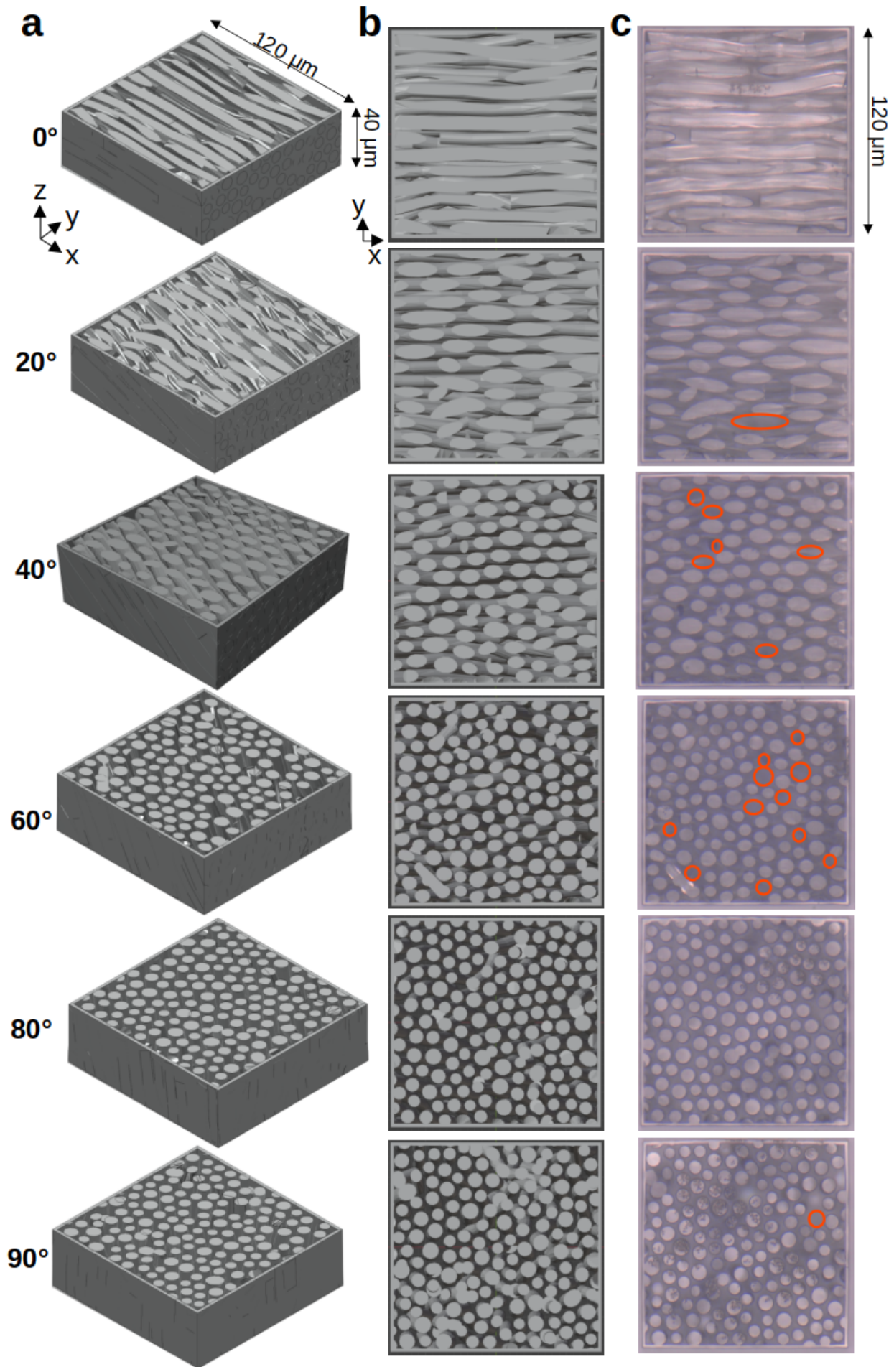
Figure A3.
Measured vervet brain sections no. 502 and 504 with anatomical annotations: corpus callosum (cc), fornix (fx), cingulum (cg), corona radiata (cr), optic tract (ot). The images show the averaged scattering signal obtained from angular ComSLI measurements; multiple tiles were stitched together to show the whole brain sections.
Figure A3.
Measured vervet brain sections no. 502 and 504 with anatomical annotations: corpus callosum (cc), fornix (fx), cingulum (cg), corona radiata (cr), optic tract (ot). The images show the averaged scattering signal obtained from angular ComSLI measurements; multiple tiles were stitched together to show the whole brain sections.
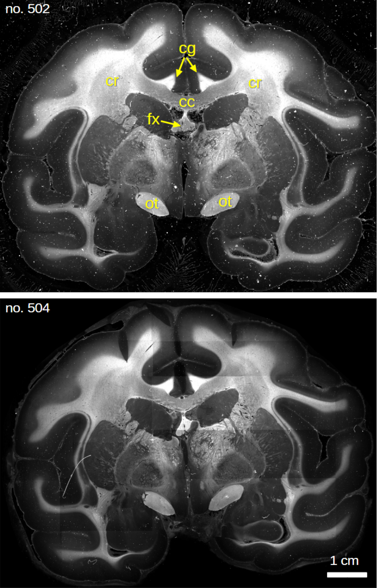
Figure A4.
Radial peak finding and peak distance of azimuthal line profiles. (a,b) Example scattering pattern and azimuthal line profile (for -inclined 3D-phantom and ). The black dots in (a) indicate the points that were evaluated to identify the points of highest intensity (red dots) for each azimuthal line profile. The graph in (b) shows both the raw data (red points) and the smoothed profile (black line) that was used to determine the peaks (black dashed lines). The magenta lines indicate the theoretical curve. (c) Scattering patterns of the 3D-printed fiber bundles for different inclination angles . The rings with and are marked by black and red circles, respectively, and the theoretical curves by red dashed lines. (d) Corresponding azimuthal line profiles for (black) and (red). (e) Azimuthal peak distance vs. inclination for (black) and (red). The inclination angles of the top part of the figure () are indicated by vertical dashed lines. (f) Inclination vs. polar illumination angle for different peak distances (colors). The red line indicates the maximum possible inclination angle that can be computed from an angular ComSLI measurement with polar illumination angle .
Figure A4.
Radial peak finding and peak distance of azimuthal line profiles. (a,b) Example scattering pattern and azimuthal line profile (for -inclined 3D-phantom and ). The black dots in (a) indicate the points that were evaluated to identify the points of highest intensity (red dots) for each azimuthal line profile. The graph in (b) shows both the raw data (red points) and the smoothed profile (black line) that was used to determine the peaks (black dashed lines). The magenta lines indicate the theoretical curve. (c) Scattering patterns of the 3D-printed fiber bundles for different inclination angles . The rings with and are marked by black and red circles, respectively, and the theoretical curves by red dashed lines. (d) Corresponding azimuthal line profiles for (black) and (red). (e) Azimuthal peak distance vs. inclination for (black) and (red). The inclination angles of the top part of the figure () are indicated by vertical dashed lines. (f) Inclination vs. polar illumination angle for different peak distances (colors). The red line indicates the maximum possible inclination angle that can be computed from an angular ComSLI measurement with polar illumination angle .
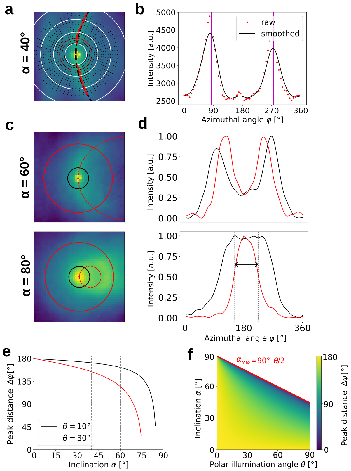
References
- Frontera, W.R.; Ochala, J. Skeletal Muscle: A Brief Review of Structure and Function. Calcif. Tissue Int. 2015, 96, 183–195. [Google Scholar] [CrossRef]
- Kesson, M.; Atkins, E. Collagen fibres. In Orthopaedic Medicine, 2 ed.; Elsevier, 2005. [Google Scholar]
- Conklin, M.W.; Eickhoff, J.C.; Riching, K.M.; Pehlke, C.A.; Eliceiri, K.W.; Provenzano, P.P.; Friedl, A.; Keely, P.J. Aligned Collagen Is a Prognostic Signature for Survival in Human Breast Carcinoma. Am. J. Pathol. 2011, 178, 1221–1232. [Google Scholar] [CrossRef]
- Amunts, K.; DeFelipe, J.; Pennartz, C.; Destexhe, A.; Migliore, M.; Ryvlin, P.; Furber, S.; Knoll, A.; Bitsch, L.; Bjaalie, J.G.; et al. Linking Brain Structure, Activity, and Cognitive Function through Computation. eNeuro 2022, 9, ENEURO.0316–21. [Google Scholar] [CrossRef]
- Cocks, E.; Taggart, M.; Rind, F.; White, K. A guide to analysis and reconstruction of serial block face scanning electron microscopy data. J. Microsc. 2018, 270, 217–234. [Google Scholar] [CrossRef]
- Peddie, C.J.; Collinson, L.M. Exploring the third dimension: Volume electron microscopy comes of age. Micron 2014, 61, 9–19. [Google Scholar] [CrossRef]
- Eberle, A.L.; Zeidler, D. Multi-Beam Scanning Electron Microscopy for High-Throughput Imaging in Connectomics Research. Front. Neuroanat. 2018, 12, 112. [Google Scholar] [CrossRef]
- Amunts, K.; Lepage, C.; Borgeat, L.; Mohlberg, H.; Dickscheid, T.; Rousseau, M.E.; Bludau, S.; Bazin, P.L.; Lewis, L.B.; Oros-Peusquens, A.M.; et al. BigBrain: An Ultrahigh-Resolution 3D Human Brain Model. Science 2013, 340, 1472–1475. [Google Scholar] [CrossRef]
- Carriel, V.; Campos, A.; Alaminos, M.; Raimondo, S.; Geuna, S. Staining Methods for Normal and Regenerative Myelin in the Nervous System. In Histochemistry of Single Molecules: Methods and Protocols;Methods in Molecular Biology; Pellicciari, C., Biggiogera, M., Eds.; Humana Press: New York, NY, 2017; Vol. 1560, pp. 207–218. [Google Scholar] [CrossRef]
- Schurr, R.; Mezer, A.A. The Glial Framework Reveals White Matter Fiber Architecture in Human and Primate Brains. Science 2021, 374, 762–767. [Google Scholar] [CrossRef]
- Khan, A.R.; Cornea, A.; Leigland, L.A.; Kohama, S.G.; Jespersen, S.N.; Kroenke, C.D. 3D Structure Tensor Analysis of Light Microscopy Data for Validating Diffusion MRI. NeuroImage 2015, 111, 192–203. [Google Scholar] [CrossRef]
- Costantini, I.; Baria, E.; Sorelli, M.; Matuschke, F.; Giardini, F.; Menzel, M.; Mazzamuto, G.; Silvestri, L.; Cicchi, R.; Amunts, K.; et al. Autofluorescence Enhancement for Label-Free Imaging of Myelinated Fibers in Mammalian Brains. Sci. Rep. 2021, 11, 8038. [Google Scholar] [CrossRef]
- Wang, H.; Lenglet, C.; Akkin, T. Structure Tensor Analysis of Serial Optical Coherence Scanner Images for Mapping Fiber Orientations and Tractography in the Brain. J. Biomed. Opt. 2015, 20, 036003. [Google Scholar] [CrossRef]
- Dell’Acqua, F.; Tournier, J.D. Modelling white matter with spherical deconvolution: How and why? NMR Biomed. 2019, 32, e3945. [Google Scholar] [CrossRef]
- Jeurissen, B.; Descoteaux, M.; Mori, S.; Leemans, A. Diffusion MRI fiber tractography of the brain. NMR Biomed. 2019, 32, e3785. [Google Scholar] [CrossRef]
- Damon, B.M.; Froeling, M.; Buck, A.K.W.; Oudeman, J.; Ding, Z.; Nederveen, A.J.; Bush, E.C.; Strijkers, G.J. Skeletal muscle diffusion tensor-MRI fiber tracking: rationale, data acquisition and analysis methods, applications and future directions. NMR Biomed. 2017, 30, e3563. [Google Scholar] [CrossRef]
- Raya, J.G.; Duarte, A.; Wang, N.; Mazzoli, V.; Jaramillo, D.; Blamire, A.M.; Dietrich, O. Applications of Diffusion-Weighted MRI to the Musculoskeletal System. J. Magn. Reson. Imaging 2024, 59, 376–396. [Google Scholar] [CrossRef]
- Wang, H.; Magnain, C.; Wang, R.; Dubb, J.; Varjabedian, A.; Tirrell, L.S.; Stevens, A.; Augustinack, J.C.; Konukoglu, E.; Aganj, I.; et al. as-PSOCT: Volumetric microscopic imaging of human brain architecture and connectivity. NeuroImage 2018, 165, 56–68. [Google Scholar] [CrossRef]
- Jones, R.; Grisot, G.; Augustinack, J.; Magnain, C.; Boas, D.A.; Fischl, B.; Wang, H.; Yendiki, A. Insight into the fundamental trade-offs of diffusion MRI from polarization-sensitive optical coherence tomography in ex vivo human brain. NeuroImage 2020, 214, 116704. [Google Scholar] [CrossRef]
- Axer, M.; Grässel, D.; Kleiner, M.; Dammers, J.; Dickscheid, T.; Reckfort, J.; Hütz, T.; Eiben, B.; Pietrzyk, U.; Zilles, K.; et al. High-Resolution Fiber Tract Reconstruction in the Human Brain by Means of Three-Dimensional Polarized Light Imaging. Front. Neuroinformatics 2011, 5, 1–13. [Google Scholar] [CrossRef]
- Schmitz, D.; Amunts, K.; Lippert, T.; Axer, M. A Least Squares Approach for the Reconstruction of Nerve Fiber Orientations from Tiltable Specimen Experiments in 3D-PLI. In Proceedings of the 2018 IEEE 15th International Symposium on Biomedical Imaging (ISBI 2018), Washington, DC, USA, 2018; pp. 132–135. [Google Scholar] [CrossRef]
- Menzel, M.; Reuter, J.A.; Grässel, D.; Costantini, I.; Amunts, K.; Axer, M. Automated computation of nerve fibre inclinations from 3D polarised light imaging measurements of brain tissue. Sci. Rep. 2022, 12, 4328. [Google Scholar] [CrossRef]
- Dohmen, M.; Menzel, M.; Wiese, H.; Reckfort, J.; Hanke, F.; Pietrzyk, U.; Zilles, K.; Amunts, K.; Axer, M. Understanding Fiber Mixture by Simulation in 3D Polarized Light Imaging. NeuroImage 2015, 111, 464–475. [Google Scholar] [CrossRef]
- Georgiadis, M.; auf der Heiden, F.; Abbasi, H.; Ettema, L.; Nirschl, J.; Taghavi, H.M.; Wakatsuki, M.; Liu, A.; Ho, W.H.D.; Carlson, M.; et al. Micron-resolution fiber mapping in histology independent of sample preparation. Nat. Commun. 2025, 16, 9572. [Google Scholar] [CrossRef]
- Abbasi, H.; Ettema, L.; van Elk, R.; Eskes, M.; Doukas, M.; Koppes, S.A.; Keereweer, S.; Menzel, M. Whole-slide mapping of tumor tissue fiber architecture via computational scattered light imaging. Biomed. Opt. Express 2026, 17, 2675–2691. [Google Scholar] [CrossRef]
- Blanke, N. Birefringence Microscopy for High-Resolution Imaging of Myelinated Axons and Myelin Pathology in the Postmortem Brain. PhD thesis, Boston University, 2023. [Google Scholar]
- Ettema, L.; Mažeika, V.; Alizadeh, M.; Abbasi, H.; Barzda, V.; Menzel, M. Fibre orientations in collagen-containing tissues revealed with computational scattered light imaging and polarimetric second harmonic generation microscopy. Sci. Rep. 2026, 16, 1047. [Google Scholar] [CrossRef]
- Georgiadis, M.; Schroeter, A.; Gao, Z.; Guizar-Sicairos, M.; Liebi, M.; Leuze, C.; McNab, J.A.; Balolia, A.; Veraart, J.; Ades-Aron, B.; et al. Nanostructure-Specific X-Ray Tomography Reveals Myelin Levels, Integrity and Axon Orientations in Mouse and Human Nervous Tissue. Nat. Commun. 2021, 12, 2941. [Google Scholar] [CrossRef]
- Silva, H.; Tassone, C.; Ross, E.G.; Lee, J.T.; Zhou, W.; Nelson, D. Collagen Fibril Orientation in Tissue Specimens From Atherosclerotic Plaque Explored Using Small Angle X-Ray Scattering. J. Biomech. Eng. 2022, 144, 024505. [Google Scholar] [CrossRef]
- Georgiadis, M.; Menzel, M.; Reuter, J.A.; Born, D.E.; Kovacevich, S.R.; Alvarez, D.; Taghavi, H.M.; Schroeter, A.; Rudin, M.; Gao, Z.; et al. Imaging Crossing Fibers in Mouse, Pig, Monkey, and Human Brain Using Small-Angle X-Ray Scattering. Acta Biomater. 2023, 164, 317–331. [Google Scholar] [CrossRef]
- Liebi, M.; Georgiadis, M.; Menzel, A.; Schneider, P.; Kohlbrecher, J.; Bunk, O.; Guizar-Sicairos, M. Nanostructure Surveys of Macroscopic Specimens by Small-Angle Scattering Tensor Tomography. Nature 2015, 527, 349–352. [Google Scholar] [CrossRef]
- Georgiadis, M.; Schroeter, A.; Gao, Z.; Guizar-Sicairos, M.; Novikov, D.S.; Fieremans, E.; Rudin, M. Retrieving neuronal orientations using 3D scanning SAXS and comparison with diffusion MRI. NeuroImage 2020, 204, 116214. [Google Scholar] [CrossRef]
- Menzel, M.; Reuter, J.; Gräßel, D.; Huwer, M.; Schlömer, P.; Amunts, K.; Axer, M. Scattered Light Imaging: Resolving the substructure of nerve fiber crossings in whole brain sections with micrometer resolution. NeuroImage 2021, 233, 117952. [Google Scholar] [CrossRef]
- Menzel, M.; Ritzkowski, M.; Reuter, J.A.; Gräßel, D.; Amunts, K.; Axer, M. Scatterometry Measurements With Scattered Light Imaging Enable New Insights Into the Nerve Fiber Architecture of the Brain. Front. Neuroanat. 2021, 15. [Google Scholar] [CrossRef]
- van Staalduine, S.; Bianco, V.; Ferraro, P.; Menzel, M. Deciphering structural complexity of brain, joint, and muscle tissues using Fourier ptychographic scattered light microscopy. VIEW 2025, 6, 20240143. [Google Scholar] [CrossRef]
- Menzel, M.; Gräßel, D.; Rajkovic, I.; Zeineh, M.M.; Georgiadis, M. Using light and X-ray scattering to untangle complex neuronal orientations and validate diffusion MRI. eLife 2023, 12. [Google Scholar] [CrossRef]
- Sporns, O. The Human Connectome: Origins and Challenges. NeuroImage 2013, 80, 53–61. [Google Scholar] [CrossRef]
- Glasser, M.F.; Smith, S.M.; Marcus, D.S.; Andersson, J.L.R.; Auerbach, E.J.; Behrens, T.E.J.; Coalson, T.S.; Harms, M.P.; Jenkinson, M.; Moeller, S.; et al. The Human Connectome Project’s Neuroimaging Approach. Nat. Neurosci. 2016, 19, 1175–1187. [Google Scholar] [CrossRef]
- Ouellette, J.N.; Drifka, C.R.; Pointer, K.B.; Liu, Y.; Lieberthal, T.J.; Kao, W.J.; Kuo, J.S.; Loeffler, A.G.; Eliceiri, K.W. Navigating the Collagen Jungle: The Biomedical Potential of Fiber Organization in Cancer. Bioengineering 2021, 8, 17. [Google Scholar] [CrossRef]
- Menzel, M.; Axer, M.; De Raedt, H.; Costantini, I.; Silvestri, L.; Pavone, F.S.; Amunts, K.; Michielsen, K. Toward a High-Resolution Reconstruction of 3D Nerve Fiber Architectures and Crossings in the Brain Using Light Scattering Measurements and Finite-Difference Time-Domain Simulations. Phys. Rev. X 2020, 10. [Google Scholar] [CrossRef]
- Nix, J.S.; Moore, S.A. What Every Neuropathologist Needs to Know: The Muscle Biopsy. J. Neuropathol. Exp. Neurol. 2020, 79, 719–733. [Google Scholar] [CrossRef]
- Aboitiz, F.; Scheibel, A.B.; Fisher, R.S.; Zaidel, E. Fiber composition of the human corpus callosum. Brain Res. 1992, 598, 143–153. [Google Scholar] [CrossRef]
- Aboitiz, F.; Ide, A.; Olivares, R. Corpus callosum morphology in relation to cerebral asymmetries in the postmortem human. In The Parallel Brain: The Cognitive Neuroscience of the Corpus Callosum; Zaidel, E., Iacoboni, M., Eds.; Massachusetts Institute of Technology, 2003; Volume chapter I.2, pp. 33–46. [Google Scholar]
- Liewald, D.; Miller, R.; Logothetis, N.; Wagner, H.J.; Schüz, A. Distribution of axon diameters in cortical white matter: an electron-microscopic study on three human brains and a macaque. Biol. Cybern. 2014, 108, 541–557. [Google Scholar] [CrossRef]
- Puetzer, J.L.; Ma, T.; Sallent, I.; Gelmi, A.; Stevens, M.M. Driving Hierarchical Collagen Fiber Formation for Functional Tendon, Ligament, and Meniscus Replacement. Biomaterials 2021, 269, 120527. [Google Scholar] [CrossRef]
- Flamourakis, G.; Dong, Q.; Kromm, D.; Teurlings, S.; van Haren, J.; Allertz, T.; Smeenk, H.; de Vrij, F.M.S.; Tas, R.P.; Smith, C.S.; et al. Deciphering the Influence of Effective Shear Modulus on Neuronal Network Directionality and Growth Cones’ Morphology via Laser-Assisted 3D-Printed Nanostructured Arrays. Adv. Funct. Mater. 2025, 35, 2409451. [Google Scholar] [CrossRef]
- Sharaf, A.; Roos, B.; Timmerman, R.; Kremers, G.J.; Bajramovic, J.J.; Accardo, A. Two-Photon Polymerization of 2.5D and 3D Microstructures Fostering a Ramified Resting Phenotype in Primary Microglia. Front. Bioeng. Biotechnol. 2022, Volume 10. [Google Scholar] [CrossRef]
- Harvey, J.; Vernold, C. Description of Diffraction Grating Behavior in Direction Cosine Space. Appl. Opt. 1998, 37, 8158–8159. [Google Scholar] [CrossRef]
- Harvey, J.; Pfisterer, R. Understanding diffraction grating behavior: including conical diffraction and Rayleigh anomalies from transmission gratings. Opt. Eng. 2019, 58, 087105. [Google Scholar] [CrossRef]
- Vankevych, P.P.; Drobenko, B.D.; Ftomyn, N.Y.; Chornodolskyy, Y.M.; Dehtiarenko, V.V.; Sliusarenko, A.V.; Chernenko, A.D.; Bolkot, P.A. Determining the position of a radiation source using the conical diffraction method. J. Phys. Stud. V. 2022, 26, 4403. [Google Scholar] [CrossRef]
- Matuschke, F.; Amunts, K.; Axer, M. fastPLI: A Fiber Architecture Simulation Toolbox for 3D-PLI. J. Open Source Softw. 2021, 6, 3042. [Google Scholar] [CrossRef]
- auf der Heiden, F.; Axer, M.; Amunts, K.; Menzel, M. Scattering polarimetry enables correlative nerve fiber imaging and multimodal analysis. Sci. Rep. 2025, 15, 18493. [Google Scholar] [CrossRef]
- Menzel, M.; Grässel, D.; Rajkovic, I.; Zeineh, M.; Georgiadis, M. Dataset: Using light and X-ray scattering to untangle complex neuronal orientations and validate diffusion MRI. 2022. [Google Scholar] [CrossRef]
- Virtanen, P.; Gommers, R.; Oliphant, T.E.; Haberland, M.; Reddy, T.; Cournapeau, D.; Burovski, E.; Peterson, P.; Weckesser, W.; Bright, J.; et al. SciPy 1.0: Fundamental Algorithms for Scientific Computing in Python. Nat. Methods 2020, 17, 261–272. [Google Scholar] [CrossRef]
- Reuter, J.A.; Menzel, M. SLIX: A Python package for fully automated evaluation of Scattered Light Imaging measurements on brain tissue. J. Open Source Softw. 2020, 5, 2675. [Google Scholar] [CrossRef]
- Shah, A.; Jhawar, S.; Goel, A.; Goel, A. Corpus Callosum and Its Connections: A Fiber Dissection Study. World Neurosurg. 2021, 151, e1024–e1035. [Google Scholar] [CrossRef]
- Decramer, T.; Swinnen, S.; van Loon, J.; Janssen, P.; Theys, T. White matter tract anatomy in the rhesus monkey: a fiber dissection study. Brain Struct. Funct. 2018, 223, 3681–3688. [Google Scholar] [CrossRef]
- Sheng, L.; Li, M.; Zheng, S.; Qi, J. Adjusting the accuracy of PEGDA-GelMA vascular network by dark pigments via digital light processing printing. J. Biomater. Appl. 2022, 36, 1173–1187. [Google Scholar] [CrossRef]
- Chang, S.Y.; Ching, T.; Hashimoto, M. Bioprinting using PEGDMA-based hydrogel on DLP printer. Mater. Today Proc. 2022, 70, 179–183. [Google Scholar] [CrossRef]
- van Altena, P.F.J.; Ransanz, L.C.; Manco, M.; Heine, V.M.; Accardo, A. Micro-digital light processing of conventional and hollow Gyroid mesoscale hydrogel scaffolds for neural cell cultures. Micro Nano Eng. 2025, 28, 100310. [Google Scholar] [CrossRef]
- Martins, I.S.; Silva, H.F.; Lazareva, E.N.; Chernomyrdin, N.V.; Zaytsev, K.I.; Oliveira, L.M.; Tuchin, V.V. Measurement of tissue optical properties in a wide spectral range: a review [Invited]. Biomed. Opt. Express 2023, 14, 249–298. [Google Scholar] [CrossRef]
- de Campos Vidal, B.; Mello, M.L.S.; Caseiro-Filho, A.C.; Godo, C. Anisotropic properties of the myelin sheath. Acta Histochem. 1980, 66, 32–39. [Google Scholar] [CrossRef]
- Menzel, M.; Pereira, S.F. Coherent Fourier scatterometry reveals nerve fiber crossings in the brain. Biomed. Opt. Express 2020, 11, 4735–4758. [Google Scholar] [CrossRef]
- Scheidt, D.; Matuschke, F.; Amunts, K.; Menzel, M.; Axer, M. Hadamard-encoded scattered light imaging for faster, signal-enhanced mapping of brain fiber orientations. Biomed. Opt. Express 2026, 17, 3854–3876. [Google Scholar] [CrossRef]
- auf der Heiden, F.; Münzer, O.; van Staalduine, S.; Amunts, K.; Axer, M.; Menzel, M. Towards high-speed computational scattered light imaging by introducing compressed sensing for optimized illumination. In Proceedings of the High-Speed Biomedical Imaging and Spectroscopy IX; Tsia, K.K., Goda, K., Eds.; International Society for Optics and Photonics, SPIE, 2024; Vol. 12853, p. 1285303. [Google Scholar] [CrossRef]
Figure 1.
Conical diffraction at an inclined grating. (a) Schematic showing the diffraction at a grating with inclination angle . (b) Predicted curves along which the diffraction orders should lie, computed for gratings with different inclinations . The gray concentric circles indicate polar steps of . (c) Azimuthal peak distance vs. inclination for different polar angles . The dashed curve indicates the polar illumination angle used in the angular ComSLI measurement. The dotted vertical/horizontal line marks the azimuthal peak distance for and (indicated by in (b)).
Figure 1.
Conical diffraction at an inclined grating. (a) Schematic showing the diffraction at a grating with inclination angle . (b) Predicted curves along which the diffraction orders should lie, computed for gratings with different inclinations . The gray concentric circles indicate polar steps of . (c) Azimuthal peak distance vs. inclination for different polar angles . The dashed curve indicates the polar illumination angle used in the angular ComSLI measurement. The dotted vertical/horizontal line marks the azimuthal peak distance for and (indicated by in (b)).
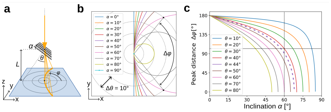
Figure 2.
Principle of Computational Scattered Light Imaging (ComSLI) measurements. (a) Light scatters perpendicularly to an in-plane fiber bundle, as can be seen in the distribution of the scattered light (scattering pattern, middle). Plotting the scattered intensity as a function of the azimuthal angle yields a scattering signal with two distinct peaks (azimuthal line profile , bottom). (b) ComSLI scatterometry measurement. The sample is illuminated by a square of LEDs which is raster-scanned over an LED display in the x- and y-direction. For every illumination position, the normally scattered light is recorded by a camera. For each pixel in the resulting image series, a scattering pattern can be reconstructed. (c) ComSLI angular measurement. The sample is illuminated by a rotating LED spot under a fixed polar angle and different azimuthal angles . For every illumination angle, the normally scattered light is recorded by a camera. For each pixel in the resulting image series, a scattering signal can be reconstructed. The top part of this figure has been adapted from Menzel et al. (2023) [36] Figure 1B and D, licensed under CC BY 4.0 (https://creativecommons.org/licenses/by/4.0/). Colors, labels, and scattering patterns have been modified.
Figure 2.
Principle of Computational Scattered Light Imaging (ComSLI) measurements. (a) Light scatters perpendicularly to an in-plane fiber bundle, as can be seen in the distribution of the scattered light (scattering pattern, middle). Plotting the scattered intensity as a function of the azimuthal angle yields a scattering signal with two distinct peaks (azimuthal line profile , bottom). (b) ComSLI scatterometry measurement. The sample is illuminated by a square of LEDs which is raster-scanned over an LED display in the x- and y-direction. For every illumination position, the normally scattered light is recorded by a camera. For each pixel in the resulting image series, a scattering pattern can be reconstructed. (c) ComSLI angular measurement. The sample is illuminated by a rotating LED spot under a fixed polar angle and different azimuthal angles . For every illumination angle, the normally scattered light is recorded by a camera. For each pixel in the resulting image series, a scattering signal can be reconstructed. The top part of this figure has been adapted from Menzel et al. (2023) [36] Figure 1B and D, licensed under CC BY 4.0 (https://creativecommons.org/licenses/by/4.0/). Colors, labels, and scattering patterns have been modified.
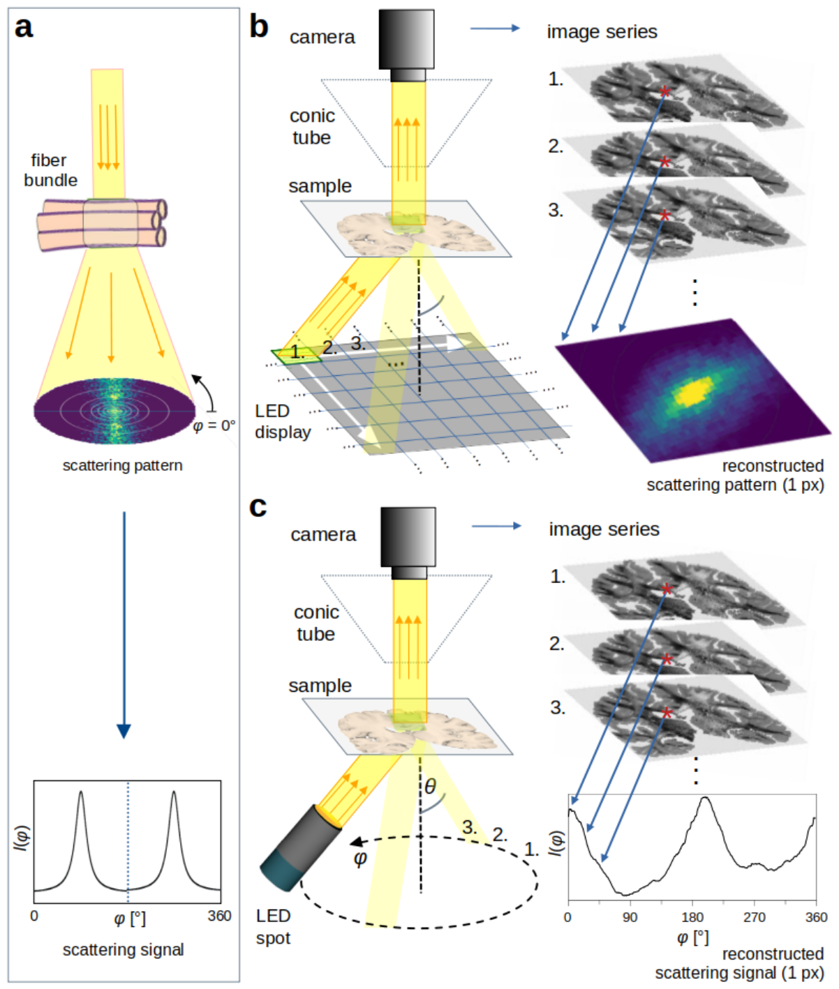
Figure 3.
Scattering patterns of 3D-printed fiber bundles for different inclination angles. (a) 3D-model, shown exemplary for . (b) Top view of the 3D-model. (c) Bright-field microscopy image of the 3D-printed phantom. The red square indicates the region in which the scattering patterns were evaluated. The scale bar is valid for both (b) and (c). (d) Scattering patterns for different inclination angles, averaged over image pixels (red square in (c)). White circles indicate steps. (e) Scattering patterns with theoretical curves (magenta) and manually annotated side lines (white dotted lines). (f) Scattering patterns with highest-intensity points (red) and fitted curves (black). (g) Comparison between theoretical curves (magenta) and fitted curves (black). (h) Fiber inclination vs. fitted inclination (including 1% RMS distance intervals). The dashed line is the theoretical expectation. (i) Normalized root-mean-square (RMS) distance between the fitted lines and the highest-intensity points for the differently inclined fiber bundles, as a function of the fitted inclination. The dotted vertical lines indicate the ranges for which the RMS distance differs from the minimum. The values for the fitted inclination, 1% RMS distance intervals, minimum RMS distance and standard deviation are listed in Appendix B, Table A1.
Figure 3.
Scattering patterns of 3D-printed fiber bundles for different inclination angles. (a) 3D-model, shown exemplary for . (b) Top view of the 3D-model. (c) Bright-field microscopy image of the 3D-printed phantom. The red square indicates the region in which the scattering patterns were evaluated. The scale bar is valid for both (b) and (c). (d) Scattering patterns for different inclination angles, averaged over image pixels (red square in (c)). White circles indicate steps. (e) Scattering patterns with theoretical curves (magenta) and manually annotated side lines (white dotted lines). (f) Scattering patterns with highest-intensity points (red) and fitted curves (black). (g) Comparison between theoretical curves (magenta) and fitted curves (black). (h) Fiber inclination vs. fitted inclination (including 1% RMS distance intervals). The dashed line is the theoretical expectation. (i) Normalized root-mean-square (RMS) distance between the fitted lines and the highest-intensity points for the differently inclined fiber bundles, as a function of the fitted inclination. The dotted vertical lines indicate the ranges for which the RMS distance differs from the minimum. The values for the fitted inclination, 1% RMS distance intervals, minimum RMS distance and standard deviation are listed in Appendix B, Table A1.
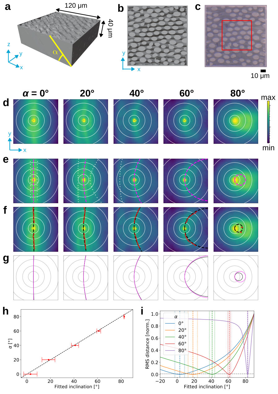
Figure 4.
Scattering patterns of a nerve fiber bundle (vervet corpus callosum) for different tilt angles . (a) Overview image of the vervet brain section (averaged scattering intensity of section no. 502). The red rectangle marks the region shown in (b). (b) Images of the sample during measurements with 0 and 60 tilt angle. The dashed vertical lines indicate the tilting axis. The scattering patterns were evaluated at the location indicated by the red dot, where fibers are mostly oriented horizontally (double-headed arrows). (c) Scattering patterns obtained for tilt angles (averaged over image pixels, indicated by the red dot in (b)). White circles indicate steps. Circular artifacts are marked by magenta arrows. (d) Calibrated scattering patterns. The center is not shown as it was not considered for the fitting. (e) Calibrated scattering patterns with highest-intensity points (red) and fitted curves (black). (f) Comparison between fitted curves (black) and theoretical curves (magenta). For the theoretical curves (theoretical -values), it was assumed that the zero-tilt fiber orientation corresponds to the average of the fitted ()-values, back-rotated to their orientation before the tilt. (g) Theoretical fiber inclination vs. fitted inclination (including 1% RMS distance intervals). The dashed line is the theoretical expectation. (h) Normalized root-mean-square (RMS) distance between the fitted line and the highest-intensity points for the different tilt angles, as a function of fitted inclination. The dotted vertical lines indicate the ranges for which the RMS distance differs from the minimum. The fitted inclination and in-plane angles, the corresponding 1% RMS distance intervals, the minimum RMS distance and standard deviation, as well as the theoretical values are listed in Appendix B, Table A2 and Table A3.
Figure 4.
Scattering patterns of a nerve fiber bundle (vervet corpus callosum) for different tilt angles . (a) Overview image of the vervet brain section (averaged scattering intensity of section no. 502). The red rectangle marks the region shown in (b). (b) Images of the sample during measurements with 0 and 60 tilt angle. The dashed vertical lines indicate the tilting axis. The scattering patterns were evaluated at the location indicated by the red dot, where fibers are mostly oriented horizontally (double-headed arrows). (c) Scattering patterns obtained for tilt angles (averaged over image pixels, indicated by the red dot in (b)). White circles indicate steps. Circular artifacts are marked by magenta arrows. (d) Calibrated scattering patterns. The center is not shown as it was not considered for the fitting. (e) Calibrated scattering patterns with highest-intensity points (red) and fitted curves (black). (f) Comparison between fitted curves (black) and theoretical curves (magenta). For the theoretical curves (theoretical -values), it was assumed that the zero-tilt fiber orientation corresponds to the average of the fitted ()-values, back-rotated to their orientation before the tilt. (g) Theoretical fiber inclination vs. fitted inclination (including 1% RMS distance intervals). The dashed line is the theoretical expectation. (h) Normalized root-mean-square (RMS) distance between the fitted line and the highest-intensity points for the different tilt angles, as a function of fitted inclination. The dotted vertical lines indicate the ranges for which the RMS distance differs from the minimum. The fitted inclination and in-plane angles, the corresponding 1% RMS distance intervals, the minimum RMS distance and standard deviation, as well as the theoretical values are listed in Appendix B, Table A2 and Table A3.
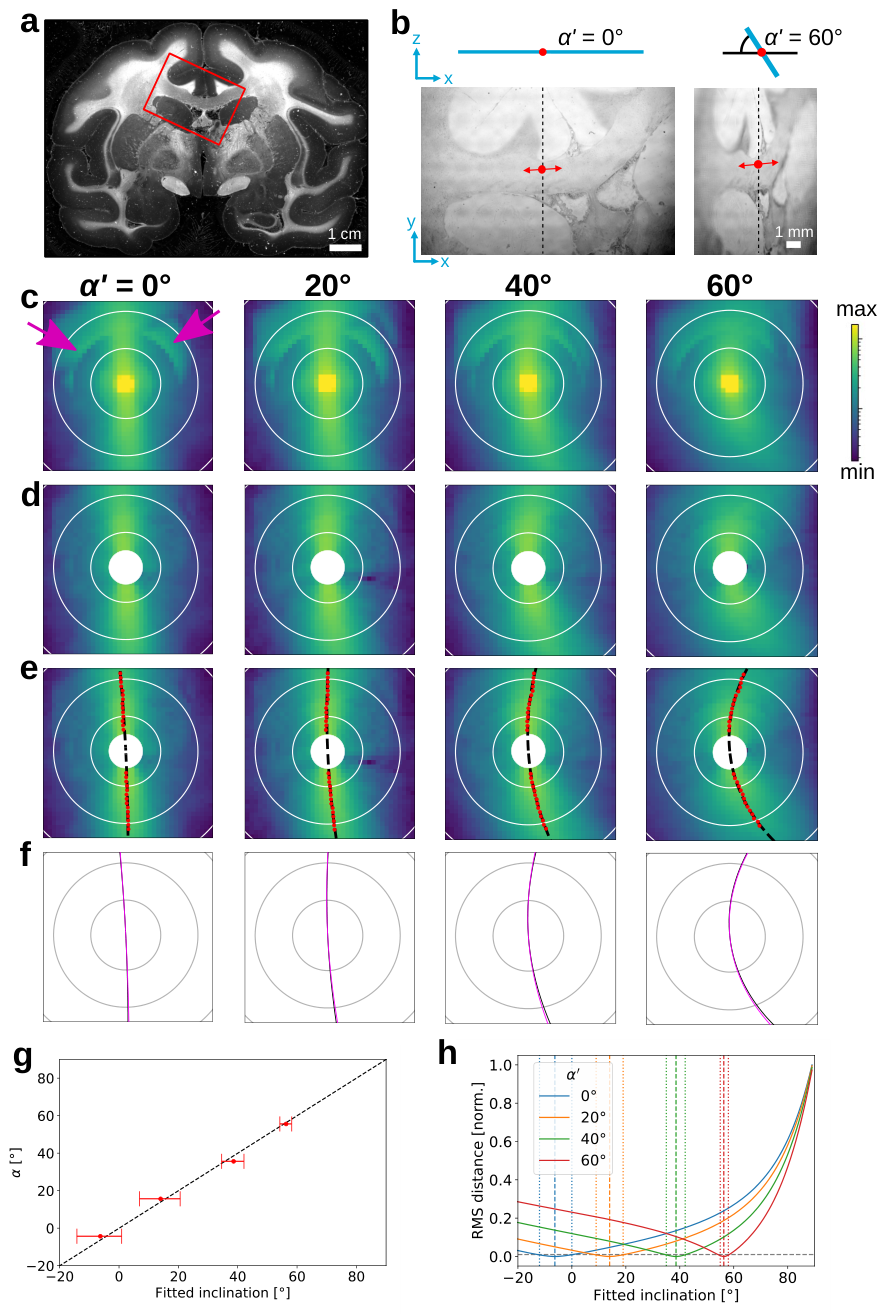
Figure 5.
Fiber inclinations of different vervet brain regions estimated from scattering patterns and azimuthal peak distances. Vervet brain section no. 504 was used for the measurements. (a) Right: Overview image of the vervet brain section (averaged scattering signal). Left: Zoom-in of the region for which the azimuthal peak distances were determined (marked by the yellow rectangle). 1, 2, 3 and 4 indicate the locations in the corpus callosum (cc – px), fornix (fx – px), bottom cingulum (cg, bottom – px) and top cingulum (cg, top – px), respectively, that were used to compute the scattering patterns. (b) Scattering pattern of the 3D-printed phantom with vertical fibers (), used for comparison. (c) Scattering patterns of the four regions with highest-intensity points (red dots), fitted curves (black dashed lines), fitted fiber inclinations , and fitted in-plane angles . The 1% RMS distance intervals, minimum and standard deviation of the root-mean-square distances are listed in Appendix B, Table A4 and Table A5. The bottom graphs show the azimuthal line profiles at (red circles) together with the azimuthal peak distances and the corresponding estimated inclinations . (d) Inclination map generated from an angular ComSLI measurement with , with the four regions from (a) indicated. (e) Inclination map generated from a 3D-scanning small-angle x-ray scattering (3D-sSAXS) measurement of an adjacent vervet brain section [53] (section no. 511, shown in Figure 6A in [36], used under CC BY 4.0). Annotations were removed and the image was cropped and mirrored at the y-axis as the brain section was measured from the other side. 3D-arrows were added to indicate the out-of-plane fiber directions in fornix and cingulum (after mirroring). Four regions (labeled 1-4) were selected for evaluation. (f) and (g) show histograms of the inclinations from the angular ComSLI and 3D-sSAXS measurements, respectively, for the four marked regions. The colored vertical lines indicate the fitted inclination values obtained from the measured scattering patterns.
Figure 5.
Fiber inclinations of different vervet brain regions estimated from scattering patterns and azimuthal peak distances. Vervet brain section no. 504 was used for the measurements. (a) Right: Overview image of the vervet brain section (averaged scattering signal). Left: Zoom-in of the region for which the azimuthal peak distances were determined (marked by the yellow rectangle). 1, 2, 3 and 4 indicate the locations in the corpus callosum (cc – px), fornix (fx – px), bottom cingulum (cg, bottom – px) and top cingulum (cg, top – px), respectively, that were used to compute the scattering patterns. (b) Scattering pattern of the 3D-printed phantom with vertical fibers (), used for comparison. (c) Scattering patterns of the four regions with highest-intensity points (red dots), fitted curves (black dashed lines), fitted fiber inclinations , and fitted in-plane angles . The 1% RMS distance intervals, minimum and standard deviation of the root-mean-square distances are listed in Appendix B, Table A4 and Table A5. The bottom graphs show the azimuthal line profiles at (red circles) together with the azimuthal peak distances and the corresponding estimated inclinations . (d) Inclination map generated from an angular ComSLI measurement with , with the four regions from (a) indicated. (e) Inclination map generated from a 3D-scanning small-angle x-ray scattering (3D-sSAXS) measurement of an adjacent vervet brain section [53] (section no. 511, shown in Figure 6A in [36], used under CC BY 4.0). Annotations were removed and the image was cropped and mirrored at the y-axis as the brain section was measured from the other side. 3D-arrows were added to indicate the out-of-plane fiber directions in fornix and cingulum (after mirroring). Four regions (labeled 1-4) were selected for evaluation. (f) and (g) show histograms of the inclinations from the angular ComSLI and 3D-sSAXS measurements, respectively, for the four marked regions. The colored vertical lines indicate the fitted inclination values obtained from the measured scattering patterns.
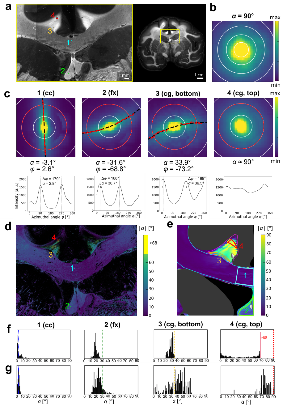
Disclaimer/Publisher’s Note: The statements, opinions and data contained in all publications are solely those of the individual author(s) and contributor(s) and not of MDPI and/or the editor(s). MDPI and/or the editor(s) disclaim responsibility for any injury to people or property resulting from any ideas, methods, instructions or products referred to in the content. |
© 2026 by the authors. Licensee MDPI, Basel, Switzerland. This article is an open access article distributed under the terms and conditions of the Creative Commons Attribution (CC BY) license (http://creativecommons.org/licenses/by/4.0/).
Copyright: This open access article is published under a Creative Commons CC BY 4.0 license, which permit the free download, distribution, and reuse, provided that the author and preprint are cited in any reuse.