

Submitted:
14 September 2026
Posted:
15 September 2026
You are already at the latest version
Abstract
Objective: Molecular measures are increasingly proposed as surrogate endpoints for evaluating gerontological interventions. Their appeal rests on two assumptions: that effects on functional outcomes are small or slow to emerge, and that molecular measures can provide valid and more detectable substitutes. Here, these assumptions are examined using simulations and empirical data. Results: Intervention effects need not occur on the timescale of the deterioration they counteract. Even when effects are small or gradual, surrogate endpoints are only one of several ways to improve detectability. Study design can do so without changing the endpoint. Even if surrogates are preferred, their validity requires that the candidate molecular measure respond to the intervention, causally influence the primary outcome under that intervention, and fully mediate the intervention’s effect on that outcome. For outcomes that are weakly constrained by selection, late-life, failure-defined, or aggregate, a small and manageable molecular surrogate set is unlikely, and one that generalizes across interventions still less so.
Keywords:
ageing
; gerontology
; surrogate endpoints
; molecular biomarkers
; clinical trial design
; causal inference
; functional outcomes
1. Introduction
Over the past decades, a large number of molecular measures of “ageing” have been proposed [1-b]. These are commonly constructed from the abundances of cellular components and their chemical modifications1 [2-a]. Early attempts relied primarily on bulk measurements from blood, whole tissues or sorted cell populations; subsequent works extended these ideas to single-cell assays. The resulting measures range from single molecular features, used on their own, to statistical composites that aggregate many of them [3-b]. These composites span simple weighted sums to highly parameterized, multi-layered models2. These molecular measures are routinely promoted for a wide range of clinical and research applications [4].
Any organism can be described by a multitude of measures. These can be derived at various scales, from molecular to whole-organism measures, and over different time frames. Each measure carries a cost: logistical, financial, temporal, or in terms of invasiveness. Some are cheap and obtained in seconds; others require years of follow-up or invasive procedures. Such measures are often nested and are linked through generative processes that unfold in space and time. Investigators aim to build models that approximate these processes. The motivation is practical: to use accessible measures to approximate less accessible ones3. One measure may be accessible but insufficiently informative for the question of interest, while another may be informative but difficult, slow, or costly to obtain. If the relationship between them can be modeled with sufficient validity, the accessible measure can be used to infer - i.e. be a surrogate of - what would otherwise require the less accessible one. It is such considerations that make molecular measures attractive in gerontology. Their broader appeal is driven, in part4, by the promise that molecular metrics can solve fundamental challenges in the evaluation of gerontological interventions [2-b][6-a]. This expectation rests on two assumptions:
- (A1)
- Effects of gerontological interventions on functional endpoints5. are expected to be small or slow to emerge, requiring large cohorts, long follow-up, or both to be detected under conventional clinical-trial designs.[1-c][3-e][5][7-b][6-b]
- (A2)
- Molecular measures can serve as valid surrogates for functional endpoints, with greater detectability of intervention effects.[3-c-d][5-b][8-a]
Assumptions are unavoidable. However, making them explicit is essential to clarify what is taken for granted, evaluate their plausibility, and revisit them when problems arise. This article evaluates these assumptions using simulations and empirical data and examines alternative approaches to evaluating gerontological interventions. First, we examine whether A1 holds across different classes of intervention. We show that functional effects need not be small or slow to emerge when interventions reverse existing deterioration. Second, even when effects are small or gradual, alternative clinical-trial designs can improve detectability without changing the endpoint. Third, with respect to A2, we examine the requirements for molecular measures to serve as valid surrogate endpoints for functional outcomes. Finally, we discuss features of age-associated deterioration that make these requirements unlikely to hold in general.
2. Methods
2.1. Notation and Terminology
Various models and simulations are used throughout this article to evaluate assumptions and classes of interventions. Abstract models are defined using generic variables (e.g. x → y). Where helpful, these are concretized using variables commonly used in the literature to provide intuition for the models’ implications. Given the multidimensional structure of biological organisms, no single metric can be assumed valid across objectives [4,9]. As such, the use of any particular variable should not be interpreted as an endorsement of its validity or general utility; variables are employed solely for illustrative purposes.
An important distinction used throughout this article is that between a statistical model M and a generative model G [10]. To simplify, this distinction is analogous to the commonly invoked difference between correlation and causation. A statistical model can be constructed between any set of variables to describe an observed relationship, but intervening on one variable does not necessarily lead to the change predicted by the model. By contrast, a generative model represents the process that gives rise to the observed relationship, in the sense that intervening on variables within the model would necessarily produce changes in other variables as specified by the model [11-a]. A given statistical model may be consistent with multiple distinct generative models , all of which reproduce the observed relationship encoded by 6. Identifying which generative process, or combination of generative processes, gives rise to a given statistical model is the objective of investigators. In some cases, an observed relationship may be well explained by a single dominant generative process. In other cases, the same statistical relationship may arise from different generative processes acting in different individuals, or from multiple processes acting simultaneously within the same individual. For example, an observed decrease in handgrip strength may reflect distinct underlying processes across individuals, such as reduced neuromuscular activation in some cases and musculoskeletal injury in others, despite producing a similar aggregate relationship between handgrip and time.
We formalize "temporal change" of an observable variable x by expressing x as a function of time t. The relationship between x and t may take several forms, including linear, exponential, constant, or more complex patterns. Depending on the choice of variable, x may increase with time (e.g. chair-rise time), decrease with time (e.g. handgrip strength), or remain approximately stable over the time window of interest (e.g. blood pH). The objective of a gerontological intervention I is to modify the relationship between a variable of interest x and time t. For the purposes of this discussion, interventions are grouped into three categories according to how they alter this relationship: reversal of the change (), halting the change (), or slowing the rate of change over time ().7
We denote by the baseline generative process of a variable x in the absence of intervention, and by the generative process under intervention I. may represent a modification of or a distinct process introduced by the intervention. The specific structure of either process is left unspecified, as the arguments do not depend on its exact form. Both may vary across variables, interventions, individuals, or contexts, and serve only as labels for the generative processes in the absence and presence of intervention.
2.2. Evaluation of Assumption A1
Assumption is a composite of two presumptions. First, intervention effects are expected to emerge on a time scale resembling that over which the deterioration originally developed. Second, if effects are small or slow to emerge, increasing sample size, extending follow-up, or both are assumed to be the principal ways to make them detectable.
Figure 1.
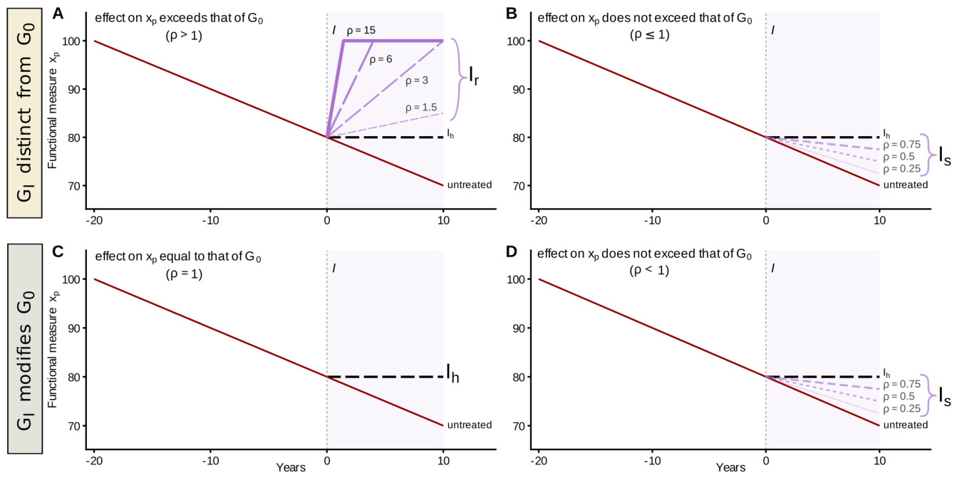
Intervention effects need not share the time scale of the decline they counteract. Each panel plots a functional measure (, e.g. handgrip strength) on the y-axis against time in years on the x-axis, with the intervention applied at year 0 (vertical dashed line, I) and the shaded band marking the post-intervention window over which treated and untreated trajectories are compared. The solid dark-red line shows the “untreated” trajectory, along which declines under the baseline generative process ; purple lines show treated trajectories under an intervention, and the black dashed horizontal line marks the trajectory of an intervention that halts further change (). Interventions are characterized by , the ratio of the magnitude of the intervention’s effect on to that of the change produced by over the same interval, which distinguishes three intervention classes: reversal (), in which recovers toward its earlier value; halting (), in which is held constant; and slowing (), in which continues to decline but at a reduced rate. Line opacity and weight scale with . Rows correspond to the relationship between the intervention process and the baseline process : distinct from (top, A–B), in which the intervention introduces a separate process that counteracts , and modifies (bottom, C–D), in which the intervention fine-tunes the parameters of rather than introducing a distinct process. (A) When is distinct and its effect on exceeds that of (), the change is reversed (), with trajectories shown for and 15; larger produces faster and more complete reversal. (B) When is distinct but its effect does not exceed that of (), the decline is slowed (), with trajectories shown for and . (C) When modifies and its effect equals that of (), the best attainable outcome is halting the decline (); reversal is not possible, as the intervention acts on the process generating the decline rather than restoring prior loss. (D) When modifies and its effect does not exceed that of (), the decline is slowed (), with trajectories shown for and . These are simplified scenarios to illustrate the point of when would share a similar time scale to .
Figure 1.
Intervention effects need not share the time scale of the decline they counteract. Each panel plots a functional measure (, e.g. handgrip strength) on the y-axis against time in years on the x-axis, with the intervention applied at year 0 (vertical dashed line, I) and the shaded band marking the post-intervention window over which treated and untreated trajectories are compared. The solid dark-red line shows the “untreated” trajectory, along which declines under the baseline generative process ; purple lines show treated trajectories under an intervention, and the black dashed horizontal line marks the trajectory of an intervention that halts further change (). Interventions are characterized by , the ratio of the magnitude of the intervention’s effect on to that of the change produced by over the same interval, which distinguishes three intervention classes: reversal (), in which recovers toward its earlier value; halting (), in which is held constant; and slowing (), in which continues to decline but at a reduced rate. Line opacity and weight scale with . Rows correspond to the relationship between the intervention process and the baseline process : distinct from (top, A–B), in which the intervention introduces a separate process that counteracts , and modifies (bottom, C–D), in which the intervention fine-tunes the parameters of rather than introducing a distinct process. (A) When is distinct and its effect on exceeds that of (), the change is reversed (), with trajectories shown for and 15; larger produces faster and more complete reversal. (B) When is distinct but its effect does not exceed that of (), the decline is slowed (), with trajectories shown for and . (C) When modifies and its effect equals that of (), the best attainable outcome is halting the decline (); reversal is not possible, as the intervention acts on the process generating the decline rather than restoring prior loss. (D) When modifies and its effect does not exceed that of (), the decline is slowed (), with trajectories shown for and . These are simplified scenarios to illustrate the point of when would share a similar time scale to .
Intervention Time Scales
The expectation of similar time scales presupposes a particular relationship between the baseline process , which produces the age-associated change in a variable x, and the process under intervention . Yet this represents only a subset of the possible relationships between them, not all of which support this expectation.
When is distinct from , it may counteract its effects on x with different temporal dynamics. At one extreme, deterioration that develops gradually over years under may be partially or fully reversed much more rapidly under . Suppose8. an autologous young heart could be grown for an individual and transplanted. Cardiac function would have taken decades to decline, yet the transplantation restored function over the much shorter time scale of the surgical intervention and recovery. This is not merely hypothetical. Existing interventions that clear age-associated accumulations illustrate the same principle. Antibodies developed against amyloid are one example. In two trials, donanemab and lecanemab substantially reduced mean amyloid PET levels within months (Figure 2). The accumulation had taken decades to build under ; it took months to reverse under . The contrast is clear in the placebo groups, where mean amyloid PET levels barely changed over the same 18 months9. At the other extreme, a distinct may only partially offset , producing slower deterioration rather than reversal. Suppose liver function declines under as dysfunctional hepatocytes accumulate, while selectively eliminates them and allows functional cells to repopulate the tissue. If elimination greatly exceeds accumulation, function may recover rapidly; if it only partially offsets accumulation, decline is merely slowed. Thus, when and are distinct, the time scale of the observed change depends on their relative effects on x, rather than being determined by the time scale of deterioration under .
The relationship typically presumed by is one in which does not introduce a distinct process but instead fine-tunes the parameters of . Suppose replication errors accumulate under . Their rate depends partly on DNA polymerase fidelity. A small molecule could allosterically increase that fidelity and thereby reduce the rate of new errors, without correcting those already present. If the accumulated errors contribute to functional decline, the intervention slows the process generating that decline rather than introducing a distinct restorative process. Consider the best case for this mode, an intervention that halts new deterioration entirely (). The detectable effect is therefore the growing separation between the treated and untreated trajectories. That separation can widen only as continues to generate deterioration in the untreated group. Even in this best case, detectability is therefore limited by the time scale of . For an intervention that only slows deterioration (), the trajectories separate more slowly still.
Detectability by Design
The second presumption is that small or slowly emerging effects make trials prohibitively costly or impractical. This follows from treating larger samples, longer follow-up, or both as the principal ways to make such effects detectable. These are indeed simple ways to increase detectability10, but they are also major contributors to trial cost and duration. The financial cost of a study scales with the number of participants enrolled and the duration over which they must be monitored and retained.
Sample size and follow-up duration, however, are only two variables within a broader study-design space—the set of variables that define how a study is conducted. The use of molecular measures as surrogates is itself one such design modification: the endpoint is changed under the assumption that molecular features provide an earlier or more sensitive readout of intervention effects. But changing the endpoint is not the only way to alter detectability. The following sections examine alternative design strategies that can improve detectability without relying on molecular surrogate endpoints. These examples are illustrative rather than exhaustive.
Study-Design Simulations
To make the study designs and their implications more intuitive, the observable variable x was taken to be handgrip strength h measured over time t. The intervention was assumed to produce a small reduction in the rate of decline (). This is the case least favorable to detection and the one most closely aligned with the presumption underlying . The objective was not to model handgrip in detail, but to compare its detectability across study designs. For each design, several analysis strategies were evaluated. Each design–analysis combination was simulated in 1000 independent trials. Detectability was defined as the proportion of trials in which the intervention effect was detected at the conventional significance threshold of p<0.05. Intuitively, it reflects the size of the intervention-induced divergence between trajectories (signal) relative to the background variation that obscures it.
Data-generating process. Each simulated individual i entered the trial at an age sampled uniformly between 65 and 80 years11Reflecting realistic recruitment windows in gerontological trials.. Handgrip strength was generated from four components: their underlying strength, an adjustment for age at trial entry, change over the course of the trial, and background variation around that trajectory. Formally,
In words,
Between-individual heterogeneity was introduced by allowing both underlying handgrip strength () and rate of change () to vary across individuals. Each was assumed to follow a Gaussian distribution around a population mean:
In words, individuals could be stronger or weaker handgrip and decline faster or slower than the population average. For simplicity, these two characteristics were treated as independent. This assumption was consistent with the BLSA data, where individual estimates of strength and rate of change were only weakly correlated (Pearson ) after centering age at the sample mean, insufficient to justify a more complex joint model given the objectives of the simulation.
Parameter calibration. To keep the simulations empirically grounded, parameters were calibrated from observed data where possible and from published estimates otherwise. The population parameters , , , and were estimated from longitudinal handgrip data from males aged 60 years and older in the Baltimore Longitudinal Study of Aging (BLSA). A Bayesian hierarchical model matching the generative structure above was fitted to these data. Age was centered at the sample mean. Posterior means were then used as fixed simulation parameters. Short-term within-individual variability could not be estimated directly from the BLSA. Repeated measurements were separated by approximately 279 days on average, making it difficult to distinguish short-term variation from genuine changes occurring between visits. We therefore calibrated using published test–retest studies of handgrip dynamometry in older adults. These report within-session coefficients of variation of approximately 5% [15–17]. At a mean handgrip strength of approximately 33 kg, this corresponds to kg. A second, more conservative value of kg (CV ) was taken from the residual variation of the BLSA model.12. Simulations were therefore run under both values to examine how increased background variation affected detectability within and across study designs.
Intervention effect. The intervention reduced the rate of handgrip decline by shifting the individual slope by . The value of was chosen so that, after two years of follow-up, the expected difference between treatment and control corresponded to Cohen’s . In other words, the simulated intervention produced a small effect relative to the natural differences in handgrip between individuals. This represents an effect that is difficult to detect under a conventional trial design.
Study designs and analysis strategies. The same dataset can often be analyzed in different ways. Some analyses use only part of the available information, while others exploit repeated measurements or comparisons within the same individual. These choices can affect detectability even when the study design itself is unchanged. Three study designs were considered:
- -
- Two-arm between-individual design. Participants were randomized to treatment and control groups, and handgrip was measured in the dominant hand at each visit. Three analysis strategies were compared: an independent-samples t-test at the final time point,13. an independent-samples t-test on change from baseline,14. and a linear mixed model (LMM) testing whether the trajectories of the two groups differed over time.15
- -
- Within-individual split-body design. This design applies when the intervention is expected to have a local effect. In other words, treating one hand is not expected to affect the other. Each participant received the intervention on the dominant hand, while the non-dominant hand served as the control. The key advantage is that treatment and control are compared within the same individual. Differences between individuals therefore contribute much less to the background variation. Two analysis strategies were compared: a paired t-test on the change scores of the treated and untreated hands,16. and an LMM testing whether the rates of change in the treated and untreated hands differed over time.
- -
- Multi-outcome between-individual design. This design applies when the intervention is expected to have a systemic effect. In other words, the intervention is expected to affect both hands. Participants were randomized to treatment and control groups as in the standard two-arm design, but both hands were measured at each visit. The key advantage is that the two hands provide correlated measurements of the same intervention effect. Combining them uses more information from each participant and reduces the influence of variation specific to either hand. Two analysis strategies were compared: an independent-samples t-test on the average change score across both hands,17. and an LMM incorporating both hands and all measurement occasions to test whether the rates of change differed between treatment and control groups.
For the latter two designs, non-dominant handgrip was modeled as 10% lower than dominant handgrip, with individual-level variation of 2 kg (SD), consistent with normative laterality data in older adults [18,19]. The rate of decline was assumed to be the same in both hands. This simplifying assumption was used to illustrate the study-design principles rather than to make claims about bilateral handgrip decline.
For each study design and analysis strategy, sample size, number of measurement occasions, and follow-up duration were varied in turn to examine how each affected detectability. All other design features were held at their default values (, three annual measurements over two years). Sample size ranged from 50 to 200, measurement occasions from 3 to 8 over a fixed two-year follow-up, and follow-up from 2 to 8 years. All simulations were repeated under both values of described above.
2.3. Evaluation of Assumption A2
Assumption (A2) is also a composite of two claims. First, a molecular variable can stand in for a primary variable in characterizing the effect of an intervention I18. Second, conditional on that validity, provides greater detectability of the intervention effect than . These claims are related but distinct. A surrogate may be valid but no easier to detect, or easier to measure but invalid. This section formalizes each claim by specifying the conditions required for it to hold. The substantive evaluation of each is left for the Discussion.
2.3.1. Validity
Consider an intervention I that produces, by stipulation, a change in a primary variable . A surrogate is valid when a decision made by observing would reach the same conclusion as one made by observing . The question is under what structural conditions this holds. Three requirements must be met under the generative process the intervention produces. We label them , , and for reference in subsequent sections.
- -
- () I produces a change in . A variable that does not respond to the intervention cannot carry information about its effect on anything else, however well-established the relationships of to may be in other contexts.
- -
- () is a cause of under . A variable is a cause of another, if intervening on the first produces a change in the second. A statistical association between the two variables, however robust, is not sufficient. If and are coupled because they share an upstream cause rather than because one produces the other, then perturbing through a route that does not engage the upstream cause will produce a change in without a corresponding change in .
- -
- () fully (or sufficiently) mediates the effect of I on . Every path by which I affects must pass through . If any path exists by which I affects without involving , then will fail to register intervention effects that nonetheless reach .
The three requirements form a hierarchy. requires only that I changes ; additionally requires that causes under ; additionally requires that all effects of I on pass through . Each therefore imposes a condition not entailed by the previous one, and the validity of as a surrogate depends on their joint satisfaction. Validity is not an intrinsic property of a measure, but is defined with respect to a particular use [4,9]. Here, that use is the substitution of for in evaluating a specific intervention I. Accordingly, the relevant causal structure is that under . It need not be the same under or another intervention . A surrogate that is valid for one intervention may therefore not be valid for another. The plausibility of these requirements for molecular measures in gerontology is evaluated in the Discussion.
2.3.2. Detectability
Conditional on validity, further assumes that the effect of I can be detected more readily through than through . This advantage is often treated as if it followed from being molecular. It does not. It depends on the specific triplet and the conditions under which the variables are measured. Greater detectability can arise in several ways. For example, the intervention-induced change in may emerge earlier [3-f] than that in , reducing the required follow-up. It may also be larger relative to the background variation in , reducing the number of observations required for detection. In other cases, may simply be easier, cheaper, or less burdensome to measure. These advantages are distinct and need not occur together. These considerations are not examined further here because they depend strongly on the particular surrogate, intervention, outcome, and measurement context. The remainder of the article focuses instead on validity, which must hold before any detectability advantage can justify the use of as a surrogate.
2.4. Code and Data Availability
The code used to generate the simulated data and produce the figures, is available in the GitHub repository associated with this project github.com/Ignophi/Molecular-Dream. The BLSA Open Data utilized in this study is available through the Alzheimer’s Disease Data Initiative (ADDI) platform. All analyses and figures were generated in R version 4.4.1. The packages Stan (v2.35.0), ggplot2 (v4.0.3), cowplot (v1.1.3), lmerTest (v3.2-1), and parallel (v4.4.1) and lme4 (v1.1-37) were used for data analysis, handling and visualization. Color palettes were specified using viridis (v0.6.5) and custom manual scales. All figure panels were modified using Inkscape.
3. Results
3.1. Two-Arm Between-Individual Design
Under default conditions (n = 50, 3 timepoints, two-year follow-up), detectability was low in the standard two-arm design across all analysis strategies (Figure 3, top row). The unpaired t-test comparing handgrip at the final timepoint showed the lowest detectability (≈0.10). The change-score unpaired t-test and the LMM yielded similar detectability (≈0.45). This reflects the fact that both approaches account for between-individual variability, which constitutes a major component of the total variance. The LMM, despite incorporating all three timepoints, did not substantially outperform the change-score t-test. This likely reflects the magnitude of the change accrued over two years relative to the background variation around each measurement, leaving the third measurement with little to add.
Figure 4.
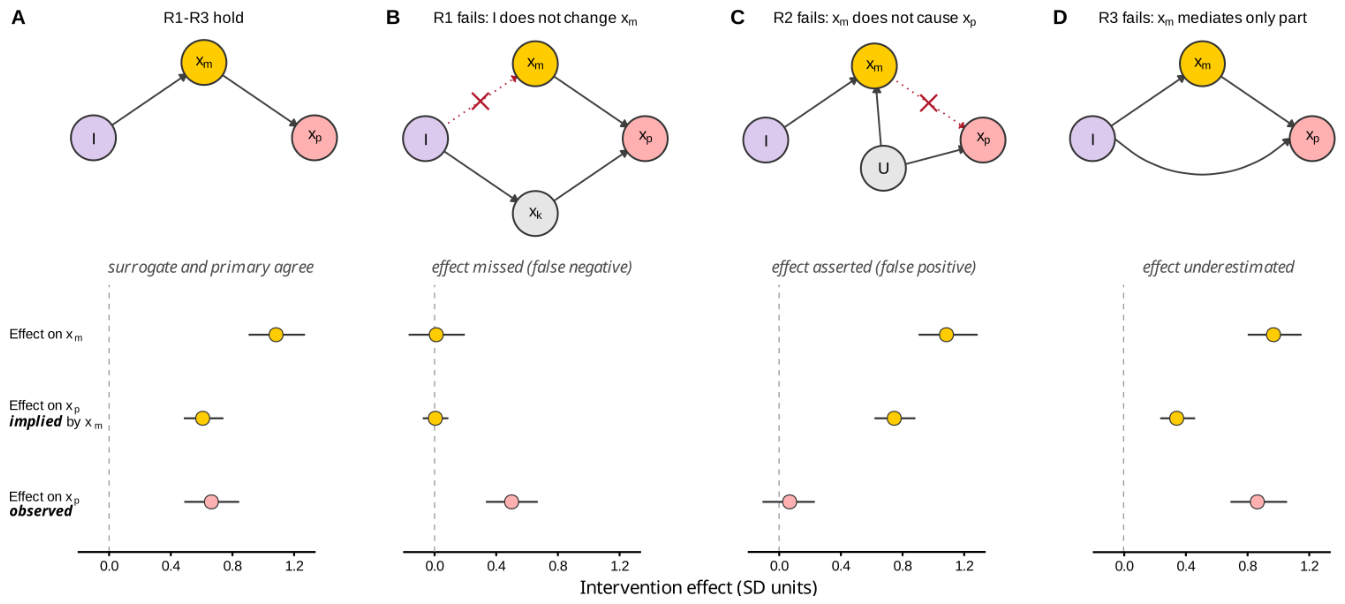
The three requirements for surrogate validity and the consequences of their failure. Each column pairs a causal diagram (top) with a forest plot of intervention effects (bottom) for one scenario. The diagrams show the causal relationships under the intervention process among the intervention (I, purple), the candidate molecular surrogate (, yellow), the primary functional outcome (, red), and, where relevant, an additional mediator (, grey) or a shared upstream cause (U, grey); solid arrows denote causal effects, and a red cross marks the absent relationship responsible for the failure. The forest plots show the intervention effect, in standard-deviation units, on the surrogate (effect on ), the effect on the primary outcome implied by (effect on implied by ), and the effect on the primary outcome actually observed (effect on observed); points are estimates and horizontal lines 95% confidence intervals, with the vertical dashed line at the null (0). (A) All three requirements hold (: I changes ; : causes under ; : fully mediates the effect of I on ): the surrogate and primary outcome agree, and the effect implied by matches the effect observed on . (B) fails, as I does not change while affecting through a separate path (via ): the surrogate registers no effect and the intervention effect is missed (false negative). (C) fails, as does not cause and the two are associated only through a shared upstream cause U: an effect on is asserted where none reaches (false positive). (D) fails, as mediates only part of the effect of I on , the remainder passing through a direct path: the effect implied by underestimates the effect observed on . These are only illustrative instances of each failure; the discrepancy between the implied and observed effect is not fixed in direction or magnitude, and a given failure can leave the surrogate showing no effect, or over- or underestimating the effect on depending on the underlying structure and parameters. Effect estimates are illustrative.
Figure 4.
The three requirements for surrogate validity and the consequences of their failure. Each column pairs a causal diagram (top) with a forest plot of intervention effects (bottom) for one scenario. The diagrams show the causal relationships under the intervention process among the intervention (I, purple), the candidate molecular surrogate (, yellow), the primary functional outcome (, red), and, where relevant, an additional mediator (, grey) or a shared upstream cause (U, grey); solid arrows denote causal effects, and a red cross marks the absent relationship responsible for the failure. The forest plots show the intervention effect, in standard-deviation units, on the surrogate (effect on ), the effect on the primary outcome implied by (effect on implied by ), and the effect on the primary outcome actually observed (effect on observed); points are estimates and horizontal lines 95% confidence intervals, with the vertical dashed line at the null (0). (A) All three requirements hold (: I changes ; : causes under ; : fully mediates the effect of I on ): the surrogate and primary outcome agree, and the effect implied by matches the effect observed on . (B) fails, as I does not change while affecting through a separate path (via ): the surrogate registers no effect and the intervention effect is missed (false negative). (C) fails, as does not cause and the two are associated only through a shared upstream cause U: an effect on is asserted where none reaches (false positive). (D) fails, as mediates only part of the effect of I on , the remainder passing through a direct path: the effect implied by underestimates the effect observed on . These are only illustrative instances of each failure; the discrepancy between the implied and observed effect is not fixed in direction or magnitude, and a given failure can leave the surrogate showing no effect, or over- or underestimating the effect on depending on the underlying structure and parameters. Effect estimates are illustrative.
Increasing sample size improved detectability across all three strategies. The unpaired t-test showed only modest gains, with detectability increasing from 0.10 at (n = 50) to 0.22 at (n = 200). In contrast, the two strategies that account for individual variability improved substantially, exceeding 0.8 detectability by n = 110 (0.83 for the LMM and 0.81 for the change-score t-test) and reaching ≈0.96 by n = 200.
Increasing the number of timepoints did not improve detectability for the endpoint or change-score t-tests, as both analyses rely only on the first and last measurements (≈0.43–0.49 for the change-score t-test and ≈0.07–0.11 for the endpoint t-test across the range). In contrast, the LMM, which uses all timepoints to model each individual’s trajectory over time, showed improved detectability as more measurements were collected within the same two-year follow-up period. This improvement was modest, increasing from ≈0.45 with three measurements per individual to ≈0.68 with eight measurements, remaining below the 0.8 threshold throughout.
Extending follow-up duration, while keeping the number of measurements (beginning, midpoint, and end) and the sample size unchanged, improved detectability across all three strategies. At the default two-year follow-up, detectability corresponded to that of the default design (≈0.44 for both the LMM and the change-score t-test). The two strategies then improved in parallel, reaching ≈0.77 at three years, crossing the 0.8 threshold shortly thereafter (≈0.88 at 3.5 years), and saturating from five years onwards (≥0.99). In contrast, the endpoint unpaired t-test benefited the least, increasing from 0.08 at two years to 0.46 at six years and 0.67 at eight years.
3.2. Within-Individual Split-Body Design
Under default conditions (n = 50, 3 timepoints, two-year follow-up), detectability was substantially higher for both analysis strategies compared to the two-arm design (≈0.77 for the paired change-score t-test and ≈0.78 for the split-body LMM, against ≈0.45 for the corresponding two-arm analyses). Achieving comparable detectability in the two-arm design required increasing the sample size to approximately n = 110. The two split-body analysis strategies performed almost identically under these conditions. This improvement arises from the use of within-individual comparisons. By treating the non-dominant hand as a control, between-individual variability in baseline strength and rate of decline is effectively removed. As a result, the noise component is reduced, increasing the signal-to-noise ratio without requiring larger samples or longer follow-up.
Increasing sample size led to a rapid increase in detectability for both strategies. Detectability exceeded 0.8 by n = 60 (0.85 for the LMM and 0.84 for the paired change-score t-test) and reached ≈0.95 by n = 80. At n = 120 both strategies were close to saturation (≈0.99), and both reached 1.00 by n = 170. The two strategies remained closely matched across the entire range, with no appreciable separation between them.
Increasing the number of timepoints did not improve detectability for the paired change-score t-test, as it relies only on the first and last measurements (≈0.76–0.78 across the range). In contrast, the LMM showed improved detectability as more measurements were collected within the same two-year follow-up period.
Extending follow-up duration, while keeping the number of measurements (beginning, midpoint, and end) and the sample size unchanged, led to a rapid increase in detectability for both strategies. Both began at the default-design value of ≈0.76–0.77 at two years, exceeded 0.8 by 2.5 years (≈0.92–0.93), approached saturation by three years (≈0.98), and reached 1.00 by four years.
3.3. Multi-Outcome Between-Individual Design
Under default conditions (n = 50, 3 timepoints, two-year follow-up), detectability in the multi-outcome design was substantially higher than in the standard two-arm design. Both the multi-outcome change-score and LMM achieved detectability of ≈0.74. This improvement arises from leveraging multiple correlated outcome measures within the same individuals. By jointly modeling these outcomes, the effective signal is amplified while measurement noise is partially averaged out, leading to a higher signal-to-noise ratio compared to single-outcome analyses.
Increasing sample size resulted in rapid gains in detectability for both analysis strategies. Detectability exceeded 0.8 by n = 60 (0.83 for the LMM and 0.82 for the change-score approach) and approached saturation (≥0.99) by n = 130. Compared to the two-arm design, this represents a substantial efficiency gain, as similar detectability levels required considerably larger sample sizes in single-outcome analyses (n = 110 to cross the same threshold).
Increasing the number of timepoints had a modest effect on detectability. As expected, the multi-outcome change-score approach showed little to no improvement, since it relies only on baseline and final measurements (≈0.73–0.76 across the range). In contrast, the multi-outcome LMM, which incorporates all repeated measures across outcomes, showed gradual improvement with additional timepoints. Detectability increased from approximately 0.75 with three measurements to around 0.92 with eight measurements, crossing the 0.8 threshold at five measurements.
Extending follow-up duration produced the steepest gains in detectability. Both strategies began at the default-design value of ≈0.72–0.73 at two years, exceeded the 0.8 threshold by 2.5 years (≈0.89–0.90), reached ≈0.95–0.96 by three years, and were effectively saturated (≥0.99) by four years.
3.4. Comparison Across Designs
Across all conditions, the standard two-arm design required substantially greater resources to achieve the same level of detectability as the alternative designs. Under default conditions, the split-body and multi-outcome designs reached ≈0.72–0.78 detectability while the best two-arm analysis reached ≈0.45. The two-arm design required roughly doubling the sample size (n = 110) or extending follow-up beyond three years. Both alternative designs crossed the 0.8 threshold at n = 60 and before 2.5 years of follow-up, and performed comparably to one another throughout, with the split-body design marginally higher across all three sweeps.
3.5. Sensitivity to Measurement Variability
The qualitative patterns described above were preserved across both levels of within-individual variability (σ ≈ 1.65 kg and σ ≈ 3.5 kg) (Figure S1). Higher variability reduced detectability across all designs but did not alter the relative ordering of designs or analysis strategies. The reduction was nonetheless substantial: under σ ≈ 3.5 kg no design reached the 0.8 threshold under default conditions, and neither the split-body nor the multi-outcome design reached it at n = 200. The threshold was crossed only by extending follow-up, at approximately 4.5 years for the split-body and multi-outcome designs and at approximately 6.5 years for the two-arm design.
4. Discussion
4.1. Necessity by Design
Claims that a method is a necessary solution often rely on an implicit framing, making them difficult to evaluate. Making this framing explicit requires three components: the objective, the approaches being considered, and their trade-offs. The promotion of molecular surrogate endpoints assumes that intervention effects unfold on the same timescale as the underlying deterioration, and therefore require large samples, long follow-up, or both to detect.
First, the premise does not apply uniformly across classes of interventions. The assumption that intervention effects unfold on the same timescale as the underlying deterioration depends on the relationship between and . It holds only for interventions that modify by halting or slowing it, or that introduce a separate process whose effect does not exceed that of . Outside these cases, intervention effects need not follow the timescale of the underlying deterioration or be small or slow to emerge.
Second, even within the class of interventions for which this assumption holds, the alternatives are implicitly restricted. The comparison is framed as one between increasing sample size or follow-up duration and adopting a surrogate endpoint. Study design encompasses a much broader set of choices. Molecular surrogates are themselves one such modification, in which the endpoint is changed under the assumption of earlier or more sensitive detection. Detectability, however, depends on the study design, not only the endpoint. It depends on the ratio of signal to noise, which can be altered through multiple design choices. Increasing follow-up, for example, increases the magnitude of the expected change and therefore the signal. Other design choices act primarily on the noise by reducing irrelevant variance. One common approach is longitudinal comparison, in which individuals are compared with themselves over time. This reduces between-individual variation and better isolates the intervention effect. For interventions that can be applied locally, another part of the same individual can serve as a control. Such designs are common in dermatology. The comparison is then between changes from baseline in the treated and untreated sites within the same individual. This controls not only for baseline differences, but also for shared sources of variability such as systemic factors, measurement conditions, or day-to-day fluctuations. Similar gains can be achieved by exploiting correlations between multiple outcomes. This is particularly intuitive for interventions expected to act systemically. For example, an oral intervention affecting muscle function would be expected to influence both left and right handgrip strength. Observing a small but consistent difference across both measures for the same individual provides stronger evidence than observing the same difference in only one. More generally, collecting multiple correlated outcomes increases the effective information obtained per participant. Although this increases data-collection costs, the marginal cost may be small relative to recruiting and following additional participants. This is especially the case with modern measurement techniques. For example, a single MRI scan can measure muscle volume across multiple body regions. If an intervention has a systemic effect, consistent changes across these regions provide stronger evidence than a change observed in only one.
Third, the feasibility advantage of molecular surrogate endpoints is often misstated. In most cases, approval based on a candidate surrogate endpoint is provisional. It therefore does not remove the need to measure the original outcome. The feasibility being referenced is instead earlier market access, where the product can be sold while the trial is still ongoing, partially offsetting its total cost. The advantage therefore does not arise from reduced measurement or study complexity. If anything, both increase. This distinction is important, as the design options discussed above are not incompatible with molecular surrogates. A surrogate endpoint can be used alongside split-body or multi-outcome designs to improve detectability and reach confirmatory approval earlier.
Taken together, the apparent necessity of molecular surrogate endpoints arises not from an inherent limitation of conventional trials, but from a particular framing of the problem. Once the objective, alternatives, and trade-offs are made explicit, molecular measures become one option among many rather than a required solution.
4.2. On the Insignificance of Small Effects
One possible response to the preceding analysis is to dispute the assumptions used in the simulations. Measurement variability may be higher, adherence poorer, or treatment effects smaller than modeled. Any simulation is indeed a manifestation of the assumptions used to construct it. The preceding section, however, took the value of detecting these effects for granted and asked only how they might be detected more efficiently. That premise is worth examining. Every introductory statistics text draws a distinction between statistical and clinical significance. Detecting a small effect more efficiently does not by itself establish that the effect is worth pursuing. An intervention whose benefit is so small that it requires years of sustained exposure before any meaningful difference becomes apparent may have limited practical value to the individual receiving it. Two common defenses are often invoked in response.
The first is an aggregation argument, which holds that individually small effect interventions, once confirmed, could be combined into a substantial additive or synergistic intervention. However, the value of a combination cannot be inferred directly from the value of its components. A combined intervention constitutes its own generative process, with distinct pharmacology, tolerability constraints, interactions [20], and risks. Interactions between interventions may be additive, sub-additive, synergistic, or antagonistic, might amplify adverse effects, or cause new ones to emerge that are absent from either intervention in isolation. If the combination is claimed to be valuable, that claim requires evidence from the combination itself, not extrapolation from its components. There is also an internal tension in this defense. If a much larger combined effect is expected, this undermines the premise that intervention effects are too small to evaluate without a surrogate.
The second is the compounding argument, which holds that a modest slowing of deterioration can become clinically meaningful if sustained long enough. As with the aggregation defense, this relies on extrapolating beyond the conditions actually tested. A trial conducted over a few years in a specific older population does not support claims about the magnitude of benefit that would accrue over decades [20-b], or whether the same effect would hold in younger populations [7-c]. Such projections assume that the intervention continues to act with similar magnitude over time, without substantial adaptation, resistance, counter-regulation, or attenuation outside the tested range. A trial conducted over several years in older adults does not by itself establish these claims. As such, the projected long-term benefit is partly a model-based extension rather than an observed result.19
This highlights a broader asymmetry. Small effects often require ambitious extrapolation to appear important. Their practical relevance is located not primarily in the observed trial result, but in what is assumed to happen beyond it. Yet validating those assumptions may require the very long and complex studies whose impracticality motivated the turn to surrogate endpoints in the first place.20. This is not to argue that small effects have no value. Well-characterized small effects may contribute to mechanistic understanding. The issue is one of prioritization under constraint. Time, funding, and personnel are finite. The relevant question is therefore not only whether an effect can be detected, but whether pursuing it is the best use of available resources [20-c]. Given the scale of gerontological challenges, priority may be better placed on interventions expected to produce larger and more consequential effects.21
4.3. On the Plausibility of Molecular Surrogates
Even if molecular surrogates are the preferred design option, their use still depends on whether they validly stand in for the primary outcome. Whether a useful mapping can be built between two measures depends on the generative process that links them. Intuitively, the relationship may be harder to model when the measures are far apart in biological scale or time. However, this is only a rule of thumb. A large separation in scale or time can still permit accurate inference: a positive pregnancy test, for example, uses a molecular measure in urine to infer not only a current organism-level state, but also likely changes over the coming months. Conversely, even "nearby" measures may make poor surrogates: a blood pressure reading taken now may poorly predict the reading taken three hours later, because both vary with stress, sleep, caffeine, posture, and measurement conditions. Relative scale, therefore, cannot by itself establish either the promise or the weakness of a candidate surrogate.
As presented in the Methods, three requirements must hold for a surrogate to be valid. requires that the intervention I produces a change in the molecular variable . This is usually the simplest requirement to evaluate. One can compare an intervention group to a control group and test whether changes in response to I. In practice, often functions as a screening criterion: variables that do not respond to the intervention are excluded as candidate surrogates. Establishing is more demanding. It requires that is a cause of under the generative process induced by the intervention, . First, the effect of on may depend on how is modified. Suppose is the abundance of a protein. The same measured increase in could be produced by delivering mRNA encoding the protein, by increasing transcription from the endogenous locus, or by inhibiting degradation of the existing protein. Each may produce the same measured abundance of , but not necessarily to the same biological state. The same change in may therefore have different effects on depending on the intervention used to generate it. The causal claim is therefore not simply about in isolation, but about the triplet .22. Second, even when the causal claim is anchored to a specific intervention, establishing it requires observing . This is precisely the measure the surrogate is meant to replace because it is costly, slow, invasive, or otherwise difficult to obtain. A controlled experiment must show that modifying through I produces the expected change in . This may be feasible for a specific triplet , but it cannot be generalized to other interventions without further validation.
The remainder of this discussion focuses primarily on , assuming and are satisfied. requires that fully or sufficiently mediates the effect of I on . Every relevant path from I to must pass through 23. Otherwise, the surrogate will not fully capture the intervention effect. In such cases, the surrogate may fail in either direction, missing effects that reach through other routes or implying a change in that does not occur. As with , must be evaluated for a specific . In principle, could be tested empirically. One could vary the magnitude of the intervention, measure both and , and ask whether intervention-induced changes in are captured by changes in . If changes when does not, then the intervention must affect through another route. If changes without the expected change in , then the observed change in is not sufficient to transmit the effect. However, as with , the resulting claim is local. It does not establish that fully mediates the effects of other interventions on , in other populations, or under other generative processes. This limits claims that "validated" molecular surrogates would make gerontological trials broadly faster, cheaper, or less dependent on primary outcomes. Such claims require the surrogate to generalize across interventions. If validity remains tied to the tested intervention, the surrogate cannot serve as a general replacement for . It can only support an earlier and conditional inference, pending direct evaluation of the primary outcome.24
Before considering specific examples, it is useful to examine the structure of biological organisms, as this bears directly on the plausibility of for some measures. The configurations biological systems occupy are not arbitrary; they are the result of constraints. Some are structural, such as the elements available in a given environment and their properties. Others arise through selection. Identifying these constraints helps determine what can be inferred about the system. A simple illustration makes this intuitive. Consider the function of "green fluorescence" (F), measured by exposing an organism to ultraviolet light and quantifying the emitted light at a defined wavelength. Suppose we observe a population of organisms that share the same level of F. Suppose first a structural constraint holds, such that green fluorescence can be produced by only a single protein, GFP1.25. Under this constraint, F permits a strong inference of the protein involved. If the organism fluoresces, GFP1 must be present and functional. Now suppose does not hold, and the same fluorescence can be produced by GFP1 and GFP2, which differ in sequence and structure but emit at the same wavelength. The inference now weakens. Observing F no longer implies the presence of GFP1. It may be produced by GFP1, GFP2, or through any combination of the two. Two organisms may match in F while differing entirely in the molecular route that produces it. The same problem remains under but at a different level. fixes the protein involved, but not how the observed level of GFP1-mediated fluorescence is achieved. The same F may be reached through a stronger promoter that increases GFP1 transcription, duplication of the GFP1 gene, slower degradation of the GFP1 protein, or a cellular context in which a lower amount of GFP1 produces higher fluorescence. The structural constraint therefore fixes the protein involved but leaves the generative route that produces F unconstrained [21-a]. Furthermore, whether holds or not, it is important to recognize that the same constraint does not support both directions of inference equally. Even when holds, knowing the organism fluoresces implies GFP1 is present; knowing GFP1 is present does not imply the organism fluoresces. The protein might be mislocalized, the surrounding tissue might absorb the emitted light, or a pigment might mask it. The observed fluorescence depends not only on GFP1 but on everything else that must hold for it to be produced and detected. Now suppose we identify a second constraint, : this organism survives only if it maintains a minimum level of F. Observing it alive therefore suggests that GFP1 is embedded in a configuration that produces detectable fluorescence. Under and together, the mapping between GFP1 and F becomes tighter in both directions. F implies GFP1 because no other protein can produce the signal. GFP1 becomes informative about F because survival has filtered for configurations in which GFP1 actually produces detectable fluorescence.
Biological organisms have, for the most part, been shaped by selection on organism-level measures: fertility, mobility, resistance to starvation, avoidance of predation, and survival long enough to reproduce. The molecular configurations that realize these properties are therefore often constrained only indirectly [21-b] [22-a-b] [23-a]. It can be favored or disfavored only insofar as it alters the measure on which selection acts, or changes the costs, risks, and trade-offs associated with producing it. A system selected in this way is under no constraint to realize a function through a single dedicated route, and may even be favored not to26. Distributing a function across multiple processes through redundancy, degeneracy27, and decentralization can confer several advantages. First, such architectures increase robustness [32-a]: the function can persist despite mutation, damage, environmental fluctuation, or perturbation of any single route. Second, they increase adaptability: different routes can be recruited as internal or external conditions change. Third, they increase evolvability [21-c] [32-b]: because the function is not tied to one indispensable route, components can vary, specialize, or acquire new roles without abolishing the original function. Fourth, they relax the demands placed on any individual component: when reliability is secured at the level of the system, cheaper, noisier, or more error-prone components can be tolerated because their failures need not propagate to the function2829. The full set of advantages is too large to treat here and would require a separate discussion. The point here is narrower. Distributed realization is not merely incidental, but an expected consequence of selection acting on organism-level properties rather than on the preservation of particular molecular routes. This weakens the expectation that a single molecular variable will generally satisfy . If an organismal property can be produced through several partially overlapping molecular routes, an intervention may affect without all of its effects passing through . Conversely, an intervention may move without moving as the system compensates through other routes. Under such architectures, may still be informative. It may report one route by which can be produced, one state of the system, or one response to a particular intervention. It should not, however, be assumed to completely mediate the intervention effect. Its validity remains local to configurations in which the causal route through is both active and necessary.
This is not to claim that biological organization always favors distributed realization. Centralization can also be favored, but under a different set of constraints. One such constraint is coordination [32-c]. When several downstream effects must occur together, and partial activation is useless or harmful, a common upstream trigger can be favored over independent ones that could act out of step. A second constraint is controllability. It is closely linked to coordination, but concerns the governance of coordinated change. A state that must be reliably entered, maintained, modulated, and exited is easier to govern when control is concentrated at a few points than when it is dispersed across many. A third constraint is signal pooling. Here a central node is favored not because it coordinates downstream effects, but because it integrates upstream information, collecting many separate inputs and resolving them into a single decision. The cellular decision of whether to divide is a clear case. A cell must weigh nutrient availability, growth signals, the integrity of its DNA, and the length of its telomeres before committing to division. These inputs need not be combined by simple summation. In many cases the decision is conjunctive, where a single unmet condition is enough to block division regardless of the others. Routing the inputs through a common decision point allows them to be resolved into one coherent outcome. Where such a node exists, molecular surrogacy becomes more plausible. If an intervention I acts on a node that is both necessary for the downstream state and the point through which the relevant information passes, then the path from I to may genuinely run through , satisfying .
As such, the plausibility of a molecular surrogate for gerontological interventions can be evaluated by considering the constraints likely to govern the surrogate and primary measures of interest. Most primary measures in gerontology, including lifespan, disease-free survival, mobility, and grip strength, are high-level organismal properties. To the extent that they have been under selection, they are likely to have been selected at the functional level, leaving the molecular routes that realize them comparatively free to vary. In some cases, especially for late-life properties whose consequences occur after reproduction, the selective constraint may be weaker still, or absent altogether. The mapping is loosened further by the fact that many gerontological measures concern deterioration or failure. The space of possible failures is usually broader than the space of preserved function. The same loss of grip strength may arise through muscle atrophy, neural decline, joint pathology, impaired metabolism, or any combination of these. Failure of survival may arise through an even larger range of routes. Furthermore, this multiplicity is not only between individuals. Within an individual, somatic selection can generate heterogeneity across tissues and cell populations. As long as function is preserved, the particular molecular route by which it is preserved need not be the same across tissues, individuals, or time. Finally, many gerontological endpoints compound these problems by being aggregate by construction. "Disease-free survival", "frailty", “mobility,” and “death” group together outcomes with different generative histories under a single measured variable. Together, these features make unlikely to hold for arbitrary gerontological interventions. A single may capture one route to or one response to I, but it is unlikely to fully mediate all relevant effects of I on the primary outcome.
4.4. Alzheimer’s and Aggregates
Alzheimer’s disease provides a particularly informative case study. First, decades of public and private investment have produced a large empirical record spanning preclinical studies, longitudinal cohorts, post-mortem studies, and, most importantly, two decades of interventional human data from randomized clinical trials. Second, the problem maps directly onto the surrogacy framework outlined above. The primary outcome, , is cognitive decline, an aggregate, failure-defined outcome that unfolds over years. The candidate surrogate, , is amyloid-β aggregation, a molecular measure, more accessible than years of cognitive follow-up and situated at what is often assumed to be a "more fundamental" layer [33]. Third, the inferential problem is narrower than for broader gerontological measures30. Cognition is one component of the broader multivariate "functional" state. This makes Alzheimer’s a comparatively favorable setting in which to evaluate molecular surrogacy.
The historical development of amyloid-β as a candidate surrogate involved a progressive expansion in both the scope and strength of the claims made about it.31. Alzheimer’s 1906 report described a single patient with unusually severe, early-onset dementia whose brain contained plaques and neurofibrillary tangles. Kraepelin subsequently named the condition “Alzheimer’s disease” and distinguished it from ordinary old-age (“senile”) dementia. Similar lesions were observed in senile dementia at roughly the same time, yet the two conditions remained separate. Only later were presenile and senile "forms" argued to reflect the same underlying process and increasingly treated as manifestations of a single disease (Blessed, Tomlinson, and Roth 1968). Attention then shifted from plaques to their molecular composition after amyloid-β was identified as a major constituent [35-a][36-a]. Subsequent observations, including links involving Down syndrome and familial Alzheimer’s disease [35-d], motivated the stronger claim that amyloid-β was causal rather than merely associated with the disease. The strongest version of this causal interpretation appeared in the amyloid cascade hypothesis (Hardy & Higgins 1992; Hardy & Selkoe 2002) [37-a]), which placed Aβ deposition at the start of the disease process and treated tangles, neuronal loss, vascular damage, and dementia as downstream consequences.
This "primary cause" interpretation, an instance of the full-mediation requirement , was central to amyloid-β’s promotion, both as a candidate surrogate and as an intervention target. If Aβ deposition sits upstream of tangles, neuronal loss, vascular damage, and cognitive decline, and all relevant effects pass through it, two things follow. First, monitoring amyloid-β would suffice to infer the state of everything downstream, including cognition. Second, more consequentially, it simplifies intervention. Even if similar levels of amyloid accumulation can arise through different upstream processes [35-b], those processes need not be targeted individually. One can instead intervene on their proposed common mediator, preventing amyloid accumulation or removing existing deposits with the expectation that the downstream pathology and cognitive decline will also be prevented or reduced. This framing motivated numerous interventions aimed at reducing amyloid levels [35-c]. Some sought to reduce Aβ production by inhibiting the enzymes involved in its generation (β- or γ-secretase) [38-a]; others aimed to prevent its aggregation or accelerate its degradation [39-a]. A further class used active immunization [40-a] or monoclonal antibodies to promote the clearance of different forms of Aβ, including soluble species and deposited plaques.
Prior to intervention, observational evidence showed that the mapping between amyloid and cognition was neither simple nor consistent. A nontrivial fraction of patients with a clinical Alzheimer’s diagnosis had no detectable amyloid, while amyloid deposition was repeatedly observed in cognitively unimpaired older adults [41-a] [42-a] [43-a] [44]. The deposit, in other words, can be absent where the outcome is present and abundant where it is not. These discordances motivated explanations based on resilience [41-b], individual thresholds, and additional comorbidities that determine whether amyloid accumulation translates into cognitive decline [41-c]. More importantly, they prompted changes in trial design. Later anti-amyloid trials increasingly required confirmed amyloid positivity in addition to cognitive impairment [36-b] [41-d] [41-e]. This restriction effectively conceded that similar cognitive decline can arise through different generative routes, only some of which involve amyloid, and narrowed enrollment to cases in which the proposed surrogate was at least present.
Interventional results complicated the mapping from amyloid to cognition further. Across several mechanistically distinct approaches, amyloid could be lowered without a consistent effect on cognition. Secretase inhibitors [45] — semagacestat [38] and avagacestat (γ-secretase), verubecestat [39], atabecestat, and lanabecestat (BACE1/β-secretase) — all reduced Aβ production. None slowed cognitive decline; several — semagacestat at its higher dose, avagacestat, atabecestat, and lanabecestat — worsened it32. Earlier monoclonal antibodies showed the same pattern. Bapineuzumab measurably reduced amyloid accumulation and phospho-tau in APOE ε4 carriers but produced no cognitive benefit in either carriers or noncarriers [36]. Solanezumab [46] likewise showed no cognitive benefit despite confirmed target engagement33. Aducanumab provided an even sharper example of this discordance [47,48]. Two nearly identical Phase 3 trials34, both initially halted for futility, later showed large reductions in plaque in both trials, yet a small cognitive benefit in one trial and none in the other. Statistically significant cognitive benefits appeared only with lecanemab and donanemab, and even here the mapping was strikingly asymmetric. Both drugs cleared amyloid almost completely. Donanemab brought roughly 80% of treated patients below the threshold used to define amyloid positivity [12], while lecanemab reduced mean amyloid below the same threshold [13]. Yet the corresponding cognitive benefit remained comparatively small, on the same order as existing symptomatic drugs35. [49]. Nor was the apparent benefit equally strong across cognitive measures within the same trials: the divergence visible on the primary composite scale was markedly weaker on ADAS-Cog for lecanemab and MMSE for donanemab [49-d].
Taken together, the Alzheimer’s case illustrates the general challenges of establishing a valid molecular surrogate for a gerontological measure. First, the same cognitive decline can be reached through more than one route. Amyloid is neither necessary nor sufficient for it. Second, restricting enrollment to a more homogeneous population of confirmed amyloid-positive patients does not settle the matter because validity is intervention-dependent. The same change in the surrogate, produced through different mechanisms, need not yield the same change in the primary measure. Third, even where a benefit did appear, the mapping between surrogate and endpoint was far from a simple proportional relationship [50,51][48-b]: near-complete clearance of amyloid corresponded to only a modest slowing of decline. None of this is particular to amyloid-β. It follows from the structure of the outcome itself. Cognition is a high-level, failure-defined trait realizable through several largely independent routes, no single one of which every intervention must traverse.
4.5. The More the Merrier
Perhaps no single molecular measure can fully mediate the effect of an intervention on a primary outcome, but a set of measures can. In the fluorescence example, if F can be produced by either GFP1 or GFP2, measuring both proteins may be sufficient to account for both routes. By extension, if an intervention affects through multiple molecular routes, one might try to measure each route. The proposal is therefore that need not be satisfied by a single , but by a set . This turns a categorical question into a quantitative one. The problem shifts from whether a surrogate exists to how large the relevant mediating set is likely to be. The size matters because the practical value of the surrogate depends on how many measures are required. A small set may be recoverable; a large one may not.
Whether the set contains one measure or many, the underlying task remains the same. In either case, the goal is to construct a model that maps accessible molecular features to a primary outcome that is difficult, costly, or impossible to observe directly. Model construction can be divided into two broad tasks.36. The first, , is to identify the measures that are relevant to the outcome. The second, , is to establish how those measures combine to produce it, thereby approximating the underlying generative process. In practice, the two are interlinked and proceed iteratively. An initial feature set predicts the outcome poorly, motivating a search for further features, a revised model, and so on.
Before considering gerontological endpoints, it is helpful to consider a simpler case. Consider a single yeast cell placed in a defined medium under fixed conditions, with the primary outcome defined as the number of cells present after one day. The goal is to construct a model that predicts this outcome from molecular measures available near the start of the experiment. This is a deliberately favorable case. The organism is unicellular; the horizon is short; the ground truth is cheap and exactly observable, requiring only a plate and a day. Consider first. A standard way to identify features relevant to an outcome is a knockout screen. Each gene is eliminated in turn and the resulting change in recorded. Here the structure discussed in relation to reappears. Because the system is degenerate and redundant, a large fraction of single-gene deletions produce no detectable change in growth under standard conditions [52]. The absence of an effect from a single-gene knockout does not establish that the gene is irrelevant to the outcome. It may be one of several routes to the same function, masked by the others. The natural remedy is to delete genes in pairs, but this expands the search space combinatorially, with no principled stopping point that guarantees completeness. That double knockouts reveal interactions absent from singles gives no assurance that triples would not reveal more. One might attempt to direct the search using similarity between components, on the expectation that similar genes share function. But degeneracy is precisely the property that dissimilar components can realize the same function, so similarity-guided search is undermined by the same structure it was meant to circumvent. Identifying the relevant inputs is thus already non-trivial in a single cell under complete gene elimination, before any harder questions concerning regulation rather than presence have been raised.
Now grant that has somehow been solved, and that every gene relevant to growth has been identified. Attention then turns to . The question of interest is no longer whether a component is present, but how its level, together with the levels of the others, determines the outcome. A series of difficulties arises, each compounded as features are added. First, the relationship between a feature and the outcome may be nonlinear. A change may have little effect over one range and a large effect beyond a threshold. Second, features interact, so the effect may depends on the values of others, and the number of possible interactions grows far faster than the number of features [53-a]. Third, the order of changes may matter. Activating one pathway before another need not be equivalent to activating them in reverse. Fourth, the duration of a change may matter as much as its magnitude. Finally, feedback and compensation mean that perturbing one feature can provoke adjustments in others, so that the system observed after a perturbation is not the system that was perturbed. Each of these difficulties expands the experimental space that must be probed to approximate the generative process. Adding features therefore does not simply add measurements. It multiplies the number of configurations, perturbations, and histories that must be observed to construct a reliable model.
All of this, moreover, holds within a single fixed context [53-b]. Medium, temperature, density, and other environmental variables are held constant, while only the internal state of the cell is allowed to vary. Yet these external variables may matter as much to as any internal feature, and the same challenges apply. First, identifying the relevant environmental variables is itself a search problem, no less demanding than that for internal features. Second, internal and external variables interact, so the two problems compound. A feature’s effect depends on the context in which it is measured, and a knockout screen conducted under one set of conditions need not remain valid under another. The space to be probed is therefore not the internal configurations alone, nor the contexts alone, but their product, and the number of possible contexts is itself open-ended.
Finally, suppose the earlier problems disappear entirely. Every relevant component is known, the state of the cell is measured perfectly, and the rules governing their interactions are fully specified. Even then, two practical constraints remain. The first is computational. Complete knowledge of a system does not imply that its future state can be derived at acceptable cost. Chess provides a familiar example. The position of every piece and the rules governing every move are known exactly. Yet determining the outcome remains computationally difficult that heuristics are used instead of exhaustive calculation. A fully specified generative model can therefore remain computationally intractable. The second constraint is economic. A surrogate model is useful only if applying it is preferable to observing the primary outcome itself. In the yeast example, the primary outcome requires little more than a plate and a day. If generating the prediction costs more than simply observing the outcome, the surrogate has no practical advantage.
As such, the plausibility of a gerontological molecular surrogate set depends on the likely size of .37. The same constraints that make a single surrogate implausible also determine how large that set might be [7-d]. As grows, identifying and validating the full set becomes progressively less plausible. At one extreme are theories in which a small number of circulating factors drive deterioration, such as "pro-ageing" factors that accumulate or "anti-ageing" factors that decline. These imply a relatively small mediating set.38. At the other extreme are theories in which deterioration emerges from the combined effects of many weakly constrained processes, none of which contributes much on its own. These imply a much larger mediating set. The constraints discussed in the previous section favor the latter possibility. Selection is weak or absent for many post-reproductive properties and often acts on the level of function rather than on a particular molecular realization. Gerontological outcomes are also frequently defined by failure or aggregate states, both of which can arise through many routes. Together, these features imply that is more likely to be large than small.
4.6. Genetic Dissection of Complex Traits
An instructive empirical precedent for this strategy - and for the hope that the relevant set might remain tractable - is the quest to identify the "genetic determinants"39. of "complex traits"40. It is a search for genomic predictors, one or more variants, of a trait of interest, often the incidence of a disease. Early successes in Mendelian genetics showed that some traits followed simple and regular patterns of inheritance consistent with discrete inherited factors. Similar patterns were later recognized in rare human diseases. By the end of the twentieth century, family-based linkage studies had mapped the responsible loci for many such diseases, among them Huntington’s disease and cystic fibrosis. These successes encouraged the expectation that a similar approach could extend to more "quantitative"41. traits and to prevalent diseases [59-a] [59-b], which showed familial resemblance of their own, if to a lesser degree. The extension proved difficult [59-c]. For heart disease, diabetes, autoimmune conditions, and psychiatric disorders, linkage findings were often inconsistent and failed to replicate [60-a] [61-a]. A prominent explanation was lack of statistical power42. [62-a]. The variants underlying these traits were assumed to exert weaker effects than those behind Mendelian disorders, leaving linkage underpowered at achievable sample sizes.
The theoretical basis for this expectation had been established much earlier. In the early twentieth century, it was disputed how such quantitative traits could be explained through Mendelian inheritance [63-a] [58-d]. It was unclear how discrete inherited factors could produce the smooth distributions observed for traits such as height and blood pressure. To address this, Fisher and others posited that such a trait is governed not by one or two factors but by a large number, each contributing a small and roughly comparable effect [63-b]. If these effects combine approximately additively, their sum, together with environmental variation, can produce a continuous and often approximately Gaussian distribution43. This hypothesized model became known as the infinitesimal model and remains central to quantitative genetics to this day. Taken literally, the model implied a daunting search to identify and disentangle a great many loci, each of minuscule effect. By the close of the twentieth century, however, there was hope that reality would prove more tractable [a [64]. A prominent expression of this optimism was the Common Disease–Common Variant (CDCV) hypothesis [65-a] [66-a] [67-a] [67-b] [60-b] [62-b]. It proposed that most common-disease risk might be attributable to common susceptibility alleles at a “modest number of loci”, with at least “modest effects”44. The argument rested on two key assumptions45. The first concerned selection. Common-disease susceptibility variants would be weakly selected against if they acted mainly after reproduction or had little effect on reproductive fitness. The second concerned population history. Modern humans descend from a “relatively small” ancestral population. Along with assumptions about mutation rates and mutation–selection equilibrium, it was posited that susceptibility variants common in the ancestral population could remain predominant as the population expanded [60-c].
The CDCV hypothesis gained prominence46. alongside the achievements of the Human Genome Project and rapid advances in sequencing, genotyping, and genomic data analysis [61-b]. Together, denser variant maps, falling costs, larger samples, and association analyses comparing allele frequencies [58-e] [58-f] [67-c] [55-b] [69-a] were expected to provide the power needed to detect the variants it posited. Their identification, in turn, was expected to improve risk prediction, enable earlier intervention, guide treatment, and reveal new therapeutic targets. Over the next two decades, genome-wide association studies identified many reproducible associations, but revealed a structure less tractable than hoped [70-a] [66-b] [71-a] [72-a] [72-b] [59-e] [55-b] [73]. For most common traits and diseases, associated variants were individually weak, increasingly numerous, and together explained only a limited share of the estimated inherited variation [62-c]. Rather than uncovering a “modest number” of loci, GWAS provided growing evidence that extensive polygenicity was the norm for “complex traits” [70-b] [63-c]. The gap between expected and actual variance explained by identified variants was reflected in debates over “missing heritability” [74-a] [75-a] [62-d].
This discrepancy prompted various responses. A first route was to build more elaborate genomic models. Chief among these are polygenic risk scores [70-c] [76-a], which aggregate the small contributions of many variants into a single predictor. These vary widely, both in the number of predictors they include, from a few to many thousands and in some cases every measured variant in the genome [70-d], and in their statistical structure and underlying assumptions. Their clinical utility, however, remains disputed [70-e]. Given their statistical nature and the way they are built, their performance is uneven and population-dependent [70-f] [72-c], further limited by poor transferability across ancestries, difficulties of calibration and standardization [70-d] [72-c], and an absence of evidence that acting on a score improves patient outcomes [h [70]. A second route was to measure more. If common variants left much unexplained, perhaps the remainder lay in what had not yet been measured. This motivated the pursuit of rarer alleles through deeper and higher-resolution sequencing [62-ef], the inclusion of structural variation such as larger deletions, insertions, inversions, and translocations [62-g], and the incorporation of further molecular layers beyond sequence, among them DNA methylation, chromatin structure, and the abundances of transcripts, proteins, and non-coding RNAs. A third route was to refine the study design itself in hopes of uncovering subtle associations. Efforts here turned to larger samples [74-b], better matching of cases and controls to account for background differences [62-h], the choice of more or less heterogeneous or different ancestral populations [62-i], the control of confounders, and a focus on phenotypes that are more reliably and easily measured.
The decades-long search for the genetic determinants of complex traits carries several lessons for molecular surrogates in gerontology. First, measurement scale alone establishes neither validity nor utility. Genomic variants occupy the same scale, yet range from highly predictive determinants of Mendelian disorders to weak and context-dependent correlates for common diseases. Success in the former did not justify generalization to the latter. Second, and most fundamentally, the case illustrates the difficulty of inferring organism-level outcomes from lower-level measurements when the underlying generative process is distributed across many components and contexts. The CDCV hypothesis was, in effect, a practical example of “the more the merrier” strategy discussed above. It was a bet that the relevant set would be tractable: a “modest” number of common variants, each of modest effect, that could be combined into a useful predictor. What emerged instead was a large and expanding set of individually weak, context-dependent associations that proved difficult to combine into a valid and useful predictor. Advances in sequencing technologies removed an observational constraint. It did not remove the inferential one. In the terms used earlier, it made candidate inputs easier to observe, but it solved neither , identifying which inputs are relevant, nor , establishing how they combine to produce the trait. This difficulty is consistent with the structural considerations discussed above. As selection constrains genomic variation through its functional consequences [73-a][22-ac][23-b][73], the resulting relationships can take several forms that complicate both () and (). First, the mapping is non-unique in both directions [58-gh]. The same trait can be produced by a wide range of genotypes, as some Mendelian disorders show through their extensive allelic heterogeneity [58-i]. Conversely, a single allele can influence many traits (pleiotropy) [77], a consequence of the hierarchical and interconnected organization of organisms. Second, most complex traits are associated with a large and growing number of alleles (polygenicity), each of small effect [78-a] [56-bc]. Third, the effect of an allele is rarely fixed. It is often contingent on the rest of the genome and on environmental context (epistasis) [55-c]. The same variant can produce different outcomes on different genetic backgrounds47. [d [22]. Even within the same genetic background, the same gene relocated elsewhere in the genome can behave differently still [79-a]. Fourth48, alleles combine in ways that need not be additive, and their effects are typically probabilistic rather than deterministic, shifting the likelihood of an outcome rather than fixing it [82-a] [83-ab] [23-c] [57-c]. Finally, compounding these difficulties, the human data available for inference are not a random sample of genotype–phenotype combinations. Natural data are already filtered: numerous layers of selection — at the level of gametes, embryos, and viable organisms — remove many combinations before they can ever be observed [84-a]. Sequencing can reveal this surviving variation with increasing completeness; it cannot, by measurement alone, reconstruct the generative map that produced it. As such, the statistical models that result are heavily dependent on the context in which they were built. Each extension may recover further signal, but also increases the dimensionality of the model, the data required to fit it, and the conditions under which it must be validated. The result is not a general molecular representation of the trait, but a statistical approximation whose usefulness remains tied to the population, trait, and objective for which it was constructed.
4.7. On the Molecular Dream
No scale of measurement is inherently superior. A measure does not become more informative merely because it is taken at a finer, or supposedly more “fundamental”, biological scale. Measures differ in cost, speed, invasiveness, logistical burden, and in how much of the underlying processes they integrate. Every measure preserves some distinctions while collapsing others. Whether the discarded distinctions matter depends on what one is trying to infer.49. Protein abundance within a cell, for example, could be inferred by modeling transcription initiation, mRNA stability, ribosome loading, translation, degradation, localization, feedback, and their interactions, or estimated from a mass-spectrometry measurement. The latter is not an impoverished representation of the molecular detail beneath it. It is the integrated result of that detail, including processes that have not been identified, measured, or modeled. What it does not allow one to infer is the particular route that produced it.50
Lifespan, widely used in gerontology [85], illustrates both sides of this trade-off. It is valued precisely because it integrates the cumulative consequences of numerous exposures, interventions, physiological processes, and failures over the period of interest. Any benefit, harm, or unforeseen side effect that materially affects survival is, by definition, incorporated into the outcome, including effects investigators did not anticipate or know to measure. Yet the same lifespan can arise through very different generative routes. An intervention that extends life, for example, need not preserve mobility, cognition, strength, or other aspects of function. It is this limitation that has motivated decades of debate over the adequacy of lifespan for characterizing gerontological interventions. As such, even if lifespan could be observed immediately and at no cost in human trials, it would still be insufficient. Functional outcomes would still need to be measured. For these outcomes, intervention effects need not be slow to emerge. Even when effects are small or slow, surrogate endpoints are only one way to improve detectability. Even when a surrogate is preferred, molecular measures are unlikely to be the most valid choice, let alone the only one. This is especially the case for measures such as lifespan or functional deterioration. For outcomes that are weakly constrained by selection, late-life, failure-defined, or aggregate, a small and manageable molecular surrogate set is unlikely. Still less likely is one whose validity generalizes across interventions. Expecting this difficulty to be overcome simply by measuring more molecular variables, constructing increasingly elaborate composites, or devoting further effort to making those composites “causal” [86] is unlikely to be fruitful in the near term. A more tractable strategy may instead be to use the integrated measures biological systems already produce at many scales, rather than attempting to reconstruct them from increasingly detailed molecular measurements.
New technologies often pass through a familiar sequence [87-a]. An initial period of rapid adoption is accompanied by broad optimism about the problems the technology might solve; this is followed by a slower period of consolidation in which its valid uses and limitations are worked out. Molecular measures in gerontology appear still to carry much of the optimism of the former stage. Yet such optimism is difficult to reconcile with what is already known. Within gerontology, the relevant organism-level outcomes arise from heterogeneous, interacting, and partially redundant and degenerate processes, making broad intervention-independent molecular surrogacy an unusually demanding objective. Outside gerontology, closely related ambitions have already been pursued in fields including genomics and molecular systematics [87-c], where increasing molecular resolution repeatedly proved insufficient to eliminate the underlying inferential problem. The difficulty, therefore, is neither unexpected nor unprecedented. Continuing to treat finer molecular measurement and modeling as though they are on the verge of overcoming it risks spending another generation rediscovering limitations for which there is already substantial reason to expect.
5. Appendix
5.1. Molecular Targets in Oncology
Oncology provides one of the clearest empirical settings for examining how selection on a trait relates to the molecular routes that realize it, and when molecularly targeted interventions are most useful. At its core, the problem can be framed as one of classification: the aim is to selectively eliminate "cancerous" cells while leaving "non-cancerous" cells unaffected51. A wide range of approaches have been developed52, most of which attempt to identify a trait that is more prevalent in tumor cells than in the rest of the body. Early chemotherapies, for example, used proliferation as the targeting rule. Many tumor cells divide frequently, so drugs that disrupt DNA replication or mitosis affect them disproportionately. This trait, however, is far from tumor-specific. Many normal cell populations, including bone marrow, intestinal epithelium, hair follicles, and skin, also divide rapidly and are affected accordingly. The well-known side effects of chemotherapy are direct expressions of this limited specificity. The objective has been to refine the targeting rule to capture as many "cancer" cells as possible while sparing "normal" cells.53
The appeal of molecular measures followed directly from this aim. Such measurements might yield better targeting rules than "broader" traits such as proliferation [89]. The general approach takes a recurring shape. Tumor and non-tumor cells are compared across many measures, typically genomic, transcriptomic, and proteomic, to identify features that are enriched, mutated, or otherwise distinctive in the tumor. A construct is then built to act on this target. The feature may serve simply as a localization rule. An antibody, ligand, or small molecule binds the target and delivers a destructive payload, such as a toxin, radionuclide, or immune effector. Alternatively, if the target is functionally important to the cancer cell, small-molecule or antibody inhibitors are used to disrupt it. The two strategies can also be combined, with a single agent serving as both targeting moiety and modulator.
The ideal scenario would be a trait present in every tumor cell, absent from every normal cell, necessary for the malignancy, and one whose loss the tumor cells cannot readily bypass. Chronic myeloid leukemia (CML) approaches this ideal.54. It is defined by a reciprocal translocation between chromosomes 9 and 22, the Philadelphia chromosome. This feature is so consistent across cases that it was identified in 1960 from gross chromosome morphology and staining alone [90]. Although initially interpreted as a deletion of chromosome 22, it was shown in 1973, with improved staining, to result from a reciprocal translocation with chromosome 9 [90-a]. Over the following decade, this rearrangement was found to join part of BCR to part of ABL1, forming a fusion gene that encodes a constitutively active tyrosine kinase. Its sufficiency to drive disease was shown when murine bone-marrow cells engineered to express BCR–ABL1 produced a CML-like disease after transplantation into mice [91-a]. This prompted a search for selective inhibitors. In 1996, imatinib55. was shown to inhibit the proliferation and tumor formation of BCR–ABL1-expressing cells. In colony-forming assays, it reduced CML-derived colonies by 92–98% while largely sparing normal cells [92]. Five years later, imatinib received accelerated approval for the treatment of CML. When administered during the chronic phase, imatinib brings life expectancy close to that of the general population. Patients diagnosed today lose, on average, fewer than three life-years to the disease, an outcome rarely achieved in cancer [93,94,95].
CML also illustrates the conditions under which the same treatment becomes less effective. The longer the disease is left untreated, the less likely imatinib is to produce a durable response; this is most evident after progression to blast phase, where responses are poorer and relapse is more common [95,96]. This is thought to result from adaptations acquired by subsets of the malignant cells. Some reduce the effectiveness of imatinib, through mutations in the kinase domain [96-b][95-c], increased expression, or amplification of the fusion gene [97,98]. Others provide alternative routes for proliferation and survival less dependent on BCR–ABL1.56. Furthermore, treatment selectively eliminates susceptible cells. As such, the malignant state becomes progressively less tied to the molecular feature that initially made it tractable. This erosion of target dependence over time reflects a more general problem. The mapping between a malignant trait and its molecular realization is rarely one-to-one. CML is only one form of leukemia, accounting for approximately 15% of adult cases [99]. Leukemia is defined at the level of the trait, as the malignant proliferation of blood-forming cells. Given the range of presentations grouped under this label, it is unsurprising that there are many ways to reach it. BCR–ABL1 is one such route. Other leukemias arise through different alterations and do not depend on it [91-b]. Even within CML, the mapping is not unique [96-c]. Depending on the location of the breakpoint in BCR, the translocation can produce the p190, p210, or p230 fusion proteins, which differ in structure, activity, and disease association [100-a][91-c]. The converse also holds: some CML-like features can be produced by other activated tyrosine kinases [93-b][101,102,103].
This same pattern is visible across oncology more broadly. Some of the clearest oncological successes occur when intervention acts before substantial heterogeneity has emerged [95-b]. Vaccination against HPV or hepatitis B, for example, acts before divergent malignant populations have arisen [104]. Gastric MALT lymphoma provides another example. In early H. pylori-positive disease, eradication of the bacterium alone can cause lymphoma regression [105]. It becomes less effective as the disease progresses and growth becomes less dependent on the initiating infection.57
Appendix 5.2. Taxonomic Molecular Dreams
Structurally similar problems in other fields can be useful guides. First, similar problems may have appeared elsewhere earlier, allowing one to learn from how the debate unfolded, which mistakes happened, and which solutions proved practical. Second, a different contextual framing of the same problem can make its implicit assumptions easier to identify and the structure more intuitive to reason about. The hope that molecular measures can provide practical substitutes for difficult organismal measures and resolve definitional disputes is not unique to gerontology. Taxonomy has had centuries-long debates over how species should be defined [106,107] [79-e] and which measurements should be used to distinguish them [106-c]. Many theoretical and operational definitions have been proposed, each privileging different features of organisms. Some emphasize reproductive compatibility, others morphology or ecology. Each came with practical and interpretive difficulties. With the rise of genomic and other molecular measures, a twofold hope emerged. First, established but difficult organism-level measurements could be replaced by more accessible molecular ones. Second, long-standing classificatory disputes could be resolved by moving classification to a more "fundamental" level of measurement.
A popular and widely used definition treats two groups as distinct species if they cannot interbreed and produce viable, fertile offspring. This criterion is often difficult to measure. Testing reproductive compatibility requires controlled crosses, appropriate conditions, and organisms that can actually be bred and followed. In many cases — extinct lineages, geographically separated populations, organisms with long generation times, or organisms whose reproductive conditions are poorly understood — the test is costly and sometimes impossible. A central aim therefore became to identify whether some genomic measure could reliably predict reproductive isolation, allowing it to serve as a species criterion in place of the direct test [87-b][108]. One early candidate was overall genetic divergence58. This, however, did not turn out to be a reliable criterion [108]. The observed relationship was inconsistent. Some reproductively isolated lineages showed little genetic divergence, whereas some highly divergent lineages remained compatible [108]. The difficulty is that reproductive compatibility requires a set of conditions to hold together. Failure of any one may be sufficient to prevent successful reproduction. Isolation may arise through behavioral incompatibility, morphological mismatch, gametic incompatibility, chromosomal differences, hybrid inviability, hybrid sterility, or ecological conditions that prevent mating in the first place. Each of these modes varies across organisms, and each may be realized through many distinct genetic configurations — morphological mismatch alone arises through an enormous variety of developmental routes. Learning a genomic predictor of reproductive isolation would therefore require a training set large enough to disentangle these generative processes. But such a set consists of the very reproductive-compatibility measurements the surrogate is meant to replace; if they were already available at scale, the surrogate would offer little. This is not to claim that such a predictor is forever out of reach. With enough data and a deeper understanding of the generative processes, it may one day be built. But it is far from the imminent practical solution the move to molecular measures was claimed to provide.
One might object that reproductive isolation is an unusually distant and complex phenotype, and that molecular measures would fare better in "simpler" organisms whose relevant traits sit closer to the molecular scale. Bacteria are the natural test case. Although molecular approaches have transformed microbiology in many ways, they did not resolve the question of what should count as a bacterial species[106-e]. Even a unicellular organism is a multivariate system, and it can be partitioned in many ways depending on which features are selected. Even if one restricts the analysis to genomic data, the number of possible classifications is enormous [107-b][106-d]. A classification can be built from one gene, several genes, selected regions of genes, or similarity across the whole genome. These classifications can agree or disagree [109-a]. Which one is more useful depends on the objective. To give an intuitive example, consider the common use of 16S rRNA. Its use rests on a specific assumption that because this gene is essential and changes slowly, differences in its sequence are taken to be informative about evolutionary distance. Even if this is granted, it does not follow that a 16S-based classification is useful for every objective [79-b]. If the objective is to predict susceptibility to a particular antibiotic, the relevant classification would more naturally depend on variants, genes, or mechanisms directly related to the antibiotic’s action. It is unlikely that more information would resolve this problem; it would more likely multiply the possible classifications while leaving their usefulness objective-dependent [87-c]. A similar pattern appears in viral taxonomy. Increasing molecular detail did not eliminate boundary problems. As one discussion of viral species notes, it was once expected that complete viral genome sequences would allow species boundaries to be read directly from the “complete viral blueprint.” This did not occur. Instead, greater sequence information made clear that percentage identity thresholds between viral species remain fuzzy rather than sharply defined. The authors summarize the broader lesson pointedly: “as the amount of information increases… the fuzziness actually increases rather than decreases.” The issue is not lack of data, but the expectation that more molecular detail will collapse an objective-dependent classification problem into a single "natural" partition [79-c].
Contrasting these unfulfilled dreams with where molecular measures were practically useful is what makes the comparison instructive. These measures transformed microbiology in many ways. Where earlier work was constrained by what could be cultured, new methods made it possible to characterize unculturable organisms [109-b]. They could also guide cultivation attempts, by inferring likely growth requirements [109-c]; disentangle cases where similar traits had convergent rather than shared processes [87-d]; provide faster diagnostics for the presence of particular genes; and let older hypotheses be re-evaluated and new ones formulated [79-d][10-a]. None of this comes close to capturing the full range of practical utility molecular approaches have had, especially in bioengineering, where such tools let us reuse what evolution refined over millennia. These technologies greatly expand what can be observed, compared, and manipulated. What they do not do is resolve problems whose main difficulty was never about the volume or resolution of measurements available [87-c].
Supplementary Materials
The following supporting information can be downloaded at the website of this paper posted on Preprints.org.
Acknowledgments
This publication is partly based on publicly available research data from The Baltimore Longitudinal Study of Aging study (BLSA) that has been made available through the Alzheimer’s Disease Data Initiative Workbench. The BLSA is supported by the Intramural Research Program (IRP) of the National Institute on Aging (NIA). The author thank the investigators, staff and participants of the BLSA study for making the data available. BLSA investigators have not contributed to nor approved, and are not in any way responsible for, the contents of this publication. The author thanks the Alzheimer’s Disease Data Initiative for access to the AD Workbench used in this study.
Correspondence
If you find any mistakes or have certain comments, I would appreciate it if you can let me know at Ignophi.Hu@pm.me.
References
-
Kriukov, D.; Efimov, E.; Gelfand, M.S.; Moskalev, A.; Khrameeva, E.E. Do we actually need aging clocks? npj Aging 2025, 12, 15.
- [a]
- This surge of interest has been fueled by the growing availability of large-scale and high-throughput profiling of omics and other biomarkers associated with aging4,5.
- [b]
- Consequently, a plethora of studies has emerged, producing numerous aging clock models trained using different and sometimes rather unconventional biomarkers: DNA methylation6,7, plasma proteins8,9, urine metabolites10, clinical blood tests11, facial images12, X-ray scans13, and many others14.
- [c]
- If our goal is to develop a surrogate endpoint for clinical trials of geroprotectors or to construct an intuitive measure that reflects an individual's overall health status, then the answer is probably yes: but only if these clocks are accurate, consistent, generalizable, and provide explicit estimation of prediction uncertainty—a level of performance achievable through rigorous and extensive validation, and through developing novel methods for clock construction and uncertainty estimation.
-
Srour, L.; Bejaoui, Y.; She, J.; Alam, T.; El Hajj, N. Deep aging clocks: AI-powered strategies for biological age estimation. Ageing Research Reviews 2025, p. 102889.
- [a]
- Epigenetic clocks (DNA methylation clocks) served as the primary driver for research on aging clocks and has spurred interest in the development of transcriptomics and metabolomics-based aging clocks.
- [b]
- Aging clocks are essential for determining the effects of longevity interventions and strategies in humans (Horvath and Raj, 2018).
-
Waziry, R.; Ryan, C.; Corcoran, D.; Huffman, K.; Kobor, M.; Kothari, M.; Graf, G.; Kraus, V.; Kraus, W.; Lin, D.; et al. Effect of long-term caloric restriction on DNA methylation measures of biological aging in healthy adults from the CALERIE trial. Nature Aging 2023, 3, 248--257.
- [a]
- The goal of our analysis was to test the effect of CALERIE intervention on biological aging. We measured biological aging from blood DNAm using published algorithms. These algorithms aim to capture the accumulation of molecular changes that underlie the progressive loss of system integrity that occurs with advancing chronological age.
- [b]
- DNAm clocks are algorithms that combine information from DNAm measurements across the genome to quantify variation in biological age.
- [c]
- New measurements that summarize biological changes occurring with aging have potential to overcome this challenge; measurements to quantify biological aging that both predict future disease, disability and mortality and can detect changes in aging processes over short timescales have potential to function as surrogate endpoints for intervention effects on healthy lifespan38,49.
- [d]
- Ultimately, establishing DunedinPACE and other DNAm measures of aging as surrogate endpoints for geroscience will require evidence that changes in DNAm measures account for intervention effects on primary healthy-aging endpoints, including incidence of chronic disease and mortality18–20.
- [e]
- A barrier to advancing translation of these therapies through human trials is that intervention studies run for months or years, but human aging takes decades to cause disease46–48. New measurements that summarize biological changes occurring with aging have potential to overcome this challenge; measurements [...] detect changes in aging processes over short timescales have potential to function as surrogate endpoints for intervention effects on healthy lifespan38,49. The methods proposed to quantify biological aging [...]
- [f]
- The purpose of DNAm analysis in CALERIE was to evaluate intervention effects at the molecular level, where aging processes are posited to originate33.
- Hu, I. House of clocks: on the misuse of ageing composite measures. bioRxiv 2025, pp. 2025--05.
-
Moqri, M.; Herzog, C.; Poganik, J.R.; Justice, J.; Belsky, D.W.; Higgins-Chen, A.; Moskalev, A.; Fuellen, G.; Cohen, A.A.; Bautmans, I.; et al. Biomarkers of aging for the identification and evaluation of longevity interventions. Cell 2023, 186, 3758--3775.
- [a]
- Hence, alternative means to quantify the accumulation of age-related molecular damage and clinical functional decline are required to test interventions targeting aging.
- [b]
- Surrogate endpoints are particularly useful when the actual desired clinical endpoint is difficult to measure or expected to manifest long after an intervention is initiated. For this reason, surrogate endpoints are highly relevant to aging, where age-related disease(s) of interest or mortality would be primary endpoints.11,15,20
- [c]
- After appropriate validation, surrogate endpoint biomarkers may be used in clinical trials as a substitute for a direct measure of how a patient or participant feels, functions, or survives15 (Figure 3).
- [d]
- Validation of biomarkers of aging for use as surrogate outcomes in clinical trials is highly desirable to reduce sample numbers and trial duration. [...] endpoints must be linked, in part, to the fundamental biology of aging, must be objectively quantifiable, and should evaluate the effect of an agent or intervention on how the patient or participant 'functions, feels, or survives' [...] Total mortality is generally not considered a candidate clinical endpoint for modern trials given issues of feasibility (e.g., sample size, duration) [...]
- [e]
- The cross-species translatability criterion favors molecular, cellular, or subcellular level biomarkers11 and disfavors organism-specific biomarkers such as the PhotoAgeClock, which is based on changes in human eye corners,96 or the FRIGHT clock, which uses measures of frailty in mice.97
- Justice, J.N.; Kritchevsky, S.B. Putting epigenetic biomarkers to the test for clinical trials. Elife 2020, 9, e58592.
-
Rolland, Y.; Sierra, F.; Ferrucci, L.; Barzilai, N.; De Cabo, R.; Mannick, J.; Oliva, A.; Evans, W.; Angioni, D.; De Souto Barreto, P.; et al. Challenges in developing Geroscience trials. Nature communications 2023, 14, 5038.
- [a]
- Mortality and longevity are outcomes that are difficult to apply in randomized controlled trials because they require long-term follow-up and large sample sizes. A study with the sole objective of lifespan extension would take decades and would be very expensive. Therefore, most clinical projects in progress employ composite outcomes monitoring for the development of diseases in addition to death. Recent synopsis by ref. 4 identified studies (in rodents or human) performed on drugs already approved by the FDA which might have geroprotective effects, particularly those potentially improving healthspan and extending lifespan.
- [b]
- Demonstrating progression in clinical phenotypes, such as the transition from robust to frail, is not feasible with small study population and short follow-up.
- [c]
- For example, some observational data suggest that young subjects with a high level of insulin-like growth factor 1 (IGF-1) are protected against chronic disease, while elderly subjects with a high level of IGF-1 have an increased incidence of age-related disease and death66. This points to the possibility that Gerotherapeutic drugs such as metformin, senolytics, IGF1, and others could be beneficial when one is old but deleterious when one is young.
- [d]
- In a narrative review, Gonçalves, et al.74, reported many promising biomarkers of frailty within each key biological determinants of the aging process15 but none has demonstrated its superiority. It is therefore more likely that a set of biomarkers (such as a set of components of SASP, GDF15, epigenetic clock, telomerase activity...), rather than a single biomarker, would be the most appropriate approach to measure the rate of aging.
-
Moqri, M.; Herzog, C.; Poganik, J.R.; Ying, K.; Justice, J.N.; Belsky, D.W.; Higgins-Chen, A.T.; Chen, B.H.; Cohen, A.A.; Fuellen, G.; et al. Validation of biomarkers of aging. Nature medicine 2024, 30, 360--372.
- [a]
- Such biomarkers could predict aging-related outcomes and could serve as surrogate endpoints for the evaluation of interventions promoting healthy aging and longevity.
- Hu, I. On apples and ageing 2024.
-
McElreath, R.; et al. Statistical rethinking: A Bayesian course with examples in R and Stan; Vol. 122, CRC press Boca Raton, FL, 2016.
- [a]
- The fact that these two variables, body size and neocortex, are correlated across species makes it hard to see these relationships, unless we account for both.
-
Lloyd, P. American, German and British antecedents to Pearl and Reed's logistic curve. Population Studies 1967, 21, 99--108.
- [a]
- As the biologist Gause observed: 'It is very well known that the differential equations derived from the curves expressed in an experiment can only be regarded as empirical expressions and they do not throw any real light on the underlying factors which control the growth of the population. The only right way to go about the investigation is a direct study of factors which control the growth rate of the population and the expression of these factors in a quantitative form.'
-
Sims, J.R.; Zimmer, J.A.; Evans, C.D.; Lu, M.; Ardayfio, P.; Sparks, J.; Wessels, A.M.; Shcherbinin, S.; Wang, H.; Monkul Nery, E.S.; et al. Donanemab in early symptomatic Alzheimer disease: the TRAILBLAZER-ALZ 2 randomized clinical trial. Jama 2023, 330, 512--527.
- [a]
- Donanemab is an immunoglobulin G1 monoclonal antibody directed against insoluble, modified, N-terminal truncated form of β-amyloid present only in brain amyloid plaques. Donanemab binds to N-terminal truncated form of β-amyloid and aids plaque removal through microglialmediated phagocytosis.11
- [b]
- LSM change in CDR-SB score at 76 weeks was 1.20 (95% CI, 1.00-1.41) with donanemab and 1.88 (95% CI, 1.68-2.08) with placebo (difference, −0.67 [95% CI, −0.95 to −0.40]; P < .001) in the low/medium tau population and 1.72 (95% CI, 1.53-1.91) with donanemab and 2.42 (95% CI, 2.24-2.60) with placebo (difference, −0.7 [95% CI, −0.95 to −0.45]; P < .001) in the combined population.
- [c]
- Donanemab treatment resulted in significantly reduced brain amyloid plaque in participants at all time points assessed, with 80% (low/medium tau population) and 76% (combined population) of participants achieving amyloid clearance at 76 weeks.
-
Van Dyck, C.H.; Swanson, C.J.; Aisen, P.; Bateman, R.J.; Chen, C.; Gee, M.; Kanekiyo, M.; Li, D.; Reyderman, L.; Cohen, S.; et al. Lecanemab in early Alzheimer's disease. New England Journal of Medicine 2023, 388, 9--21.
- [a]
- After 18 months of treatment in the amyloid substudy, the mean amyloid level of 22.99 centiloids in the lecanemab group was below the threshold for amyloid positivity of approximately 30 centiloids, above which participants are considered to have elevated brain
- [b]
- In the substudy of amyloid burden on PET (a key secondary end point) involving 698 participants, the mean amyloid level at baseline was 77.92 centiloids in the lecanemab group and 75.03 centiloids in the placebo group. The adjusted mean change from baseline at 18 months was −55.48 centiloids in the lecanemab group and 3.64 centiloids in the placebo group (difference, −59.12 centiloids; 95% CI, −62.64 to −55.60; P<0.001) (Fig. 2B and Table 2).
- [c]
- The mean CDR-SB score at baseline was approximately 3.2 in both groups. The adjusted least-squares mean change from baseline at 18 months was 1.21 with lecanemab and 1.66 with placebo (difference, −0.45; 95% confidence interval [CI], −0.67 to −0.23; P<0.001). In a substudy involving 698 participants, there were greater reductions in brain amyloid burden with lecanemab than with placebo (difference, −59.1 centiloids; 95% CI, −62.6 to −55.6).
- Jack Jr, C.R.; Wiste, H.J.; Lesnick, T.G.; Weigand, S.D.; Knopman, D.S.; Vemuri, P.; Pankratz, V.S.; Senjem, M.L.; Gunter, J.L.; Mielke, M.M.; et al. Brain β-amyloid load approaches a plateau. Neurology 2013, 80, 890--896.
-
Venegas-Carro, M.; Kramer, A.; Moreno-Villanueva, M.; Gruber, M. Test-retest reliability and sensitivity of common strength and power tests over a period of 9 weeks. Sports 2022, 10, 171.
- [a]
- According to the ICC test, all comparisons of the different sessions (all three or paired across sessions) presented excellent reliability (ICC > 0.90) and a small within-subject variability or typical error for both the Avg and the Hv results (CV 2.2–6.7%).
-
Nolan, H.; O'Connor, J.D.; Donoghue, O.A.; Savva, G.M.; O'Leary, N.; Kenny, R.A. Factors affecting reliability of grip strength measurements in middle aged and older adults. HRB Open Research 2020, 3, 32.
- [a]
- All ICC point estimates were >0.9. The between-assessment ICC for dominant and non-dominant hands is typically between 0.92 and 0.93, while aggregate measure ICCs are about 0.96.
- [b]
- This analysis is based on 130 participants (median age 66 years, range 50–89 years; 55% female). Grip strength data was available at baseline and repeat assessments for 123 participants, with 21 of these having incomplete data at one or both the assessments due to injury (Figure 1). The 95% limits of agreement between baseline and repeat assessments were -6.2–7.0 kg for mean grip strength and -5.9–6.5 kg for maximum grip strength (Figure 2).
-
Bohannon, R.W.; Schaubert, K.L. Test-retest reliability of grip-strength measures obtained over a 12-week interval from community-dwelling elders. Journal of hand therapy 2005, 18, 426--428.
- [a]
- The measurements tended to decrease slightly, but not significantly, on both the left (mean decrease = 3.4 N, p = 0.500) and right (mean decrease = 8.5 N, p = 0.206) sides. The intraclass correlation coefficients (0.912 and 0.954) were consistent, with excellent reliability. The technical errors of measurement (15.8 and 21.3 N) were quite small.
-
Cuyul-Vásquez, I.; Castillo-Vejar, L.; Garrido-Muñoz, N.; Soto-Rodríguez, F.; Bascour-Sandoval, C.; Muñoz-Poblete, C.; de Souza, D.R.; Hirabara, S.M.; Curi, R.; Marzuca-Nassr, G.N. One third of people exert greater handgrip strength with their non-dominant hand. Scientific Reports 2025, 16, 1040.
- [a]
- Table 2. Differences between females and males in handgrip strength and health-related quality of life. ND: Non-dominant; D: Dominant; Kg: Kilograms, SD: Standard deviation; CI: Confidence Interval. Effect size measured with Cohen D: *Small, ** Medium, *** Large.
- [b]
- Although handgrip strength is typically greater on the dominant side, the difference between sides varies widely among studies despite published testing recommendations31–33. Furthermore, the "10% rule" may not necessarily apply to left-handed or ambidextrous individuals34,35. Ozcan et al. (2004) found that left-handed subjects have symmetrical grip strength, manual dexterity and pressure pain threshold performance compared with the asymmetrical performance observed in right-handed subjects36. These results may in part be due to lefthanded populations living in a mostly right-hand designated environment, developing better coordinated nondominant arm control36.
-
Zadoń, H.; Nowakowska-Lipiec, K.; Filipek, M.; Lepiarczyk, I.; Matusiak, A.; Piechnik, A.; Pieniażek, W.; Piejak, Z.; Przybylska, M.; Zadoń, M.; et al. Analyzing Grip Strength Disparities Between Dominant and Non-Dominant Hands: Influence of Sex and Age in the Polish Population. Applied Sciences 2025, 15, 12657.
- [a]
- When analyzing the percentage distribution of handgrip strength asymmetry levels by sex (Table 6), it was observed that both women and men most frequently exhibited asymmetry levels ≤10%. For participants with a stronger dominant hand, the percentage distribution was similar in both groups: asymmetry ≤10% occurred in 44–46% of individuals, asymmetry between 11–20% in 23–26%, and asymmetry >20% in 30–35% of participants. In contrast for those with a stronger non-dominant hand, sex-related differences were noted. Men more often demonstrated asymmetry ≤10%, while women more frequently showed asymmetry >20% (13% of women vs. 5% of men).
- [b]
- A comparison of the differences in grip strength between the dominant and nondominant limbs in this study shows that the level of asymmetry observed in the Polish population is consistent with that reported in other international studies. In the 18–35 age group, the average difference was 12%, while in people over 50, it was 10%. These results are similar to those of a meta-analysis which showed that the dominant limb is, on average, 11.6% stronger than the non-dominant limb [32].
-
Keys, M.T.; Hallas, J.; Miller, R.A.; Suissa, S.; Christensen, K. Emerging uncertainty on the anti-aging potential of metformin. Ageing research reviews 2025, 111, 102817.
- [a]
- However, evidence for reductions in major cardiovascular events or mortality from intensive glucose control with metformin is mostly derived from a subgroup of a clinical trial conducted over 30 years ago.115–117 [...] More recent meta-analyses of clinical trials of glucose-lowering medications have suggested that metformin may be neutral with respect to most cardiovascular event outcomes and mortality.119–122 Evidence of benefit is therefore generally currently regarded as being uncertain - a point echoed by leading diabetes and cardiovascular associations.123–125.
- [b]
- Even within metformin's indication for type II diabetes, its often-presumed long-term cardiovascular benefits are also not entirely certain – a point echoed by leading European and American diabetes and cardiovascular associations.
- [c]
- Three small clinical trials have assessed the short-term effects of metformin on functioning and quality of life in the context of prefrailty or frailty, with mixed results.169–171 [...] In the most recent MET-PREVENT trial, metformin for 4 months did not improve grip strength, walking speed, physical performance, muscle mass, quality of life, or activities of daily living.171 [...] the MET-PREVENT trial [...] reported that metformin was poorly tolerated by the study population.
-
Tononi, G.; Sporns, O.; Edelman, G.M. Measures of degeneracy and redundancy in biological networks. Proceedings of the National Academy of Sciences 1999, 96, 3257--3262.
- [a]
- A constrained set of outputs such as specific changes in the levels of second messengers or in gene expression thus can be brought about by a large number of different input combinations.
- [b]
- Because evolutionary selective pressure typically is applied to a long series of events involving many interacting elements at multiple temporal and spatial scales, it is unlikely that well-defined functions can be neatly assigned to independent subsets of elements or processes in biological networks. [...] Locomotion will be affected, but many other functions influenced by these structures also will likely be affected in parallel, resulting in a concomitant increase in the degeneracy of the system.
- [c]
- Similarly, the deletion of a particular gene in so-called knockout experiments often has no apparent phenotypic consequence. On the other hand, changes in the context may reveal functionally important interactions [...] The ability of natural selection to give rise to a large number of nonidentical structures capable of producing similar functions appears to increase both the robustness of biological networks and their adaptability to unforeseen environments by providing them with a large repertoire of alternative functional interactions.
-
Weiss, K.M.; Fullerton, S.M. Phenogenetic drift and the evolution of genotype-phenotype relationships. Theoretical population biology 2000, 57, 187--195.
- [a]
- However, selection acts on phenotypes, not genotypes, with no theoretically necessary connection between them. Equivalent genetic mechanisms may be associated with the same phenotype and over time phenogenetic drift, that is, drift in the relationship between genotypes and a given phenotype, can occur, even when a trait is conserved by strong and persistent selection.
- [b]
- Caveats that organisms rather than genes are the direct object of selection notwithstanding (Mayr, 1997), in practice this view treats present-day phenotypes as if they ultimately have a genetic raison d'etre.
- [c]
- It may seem mystical to suggest that biology is not "molecular" at its core the way physics and chemistry are. But suppose it is not the genome that is especially conserved by evolution. [...] Genes would then be "only" the meandering spoor left by the process of evolution by phenotype. Perhaps we have hidden behind the Modern Synthesis, and the idea that all the action is in gene frequencies, for too long. Life is ultimately about phenotypes, [...]
- [d]
- Illustrating this is the extensive extrapolation, or post hoc interpretation, of results from experiments on animal models [...] fits our expectations, it is accepted as good, e.g., mouse == human. If the experiment fails to fit our expectations, energetic hand-waving is proffered about "genetic background" to explain away the unwanted results [...] In fact, the frequent strain-dependence of such results shows clearly that within the range of mouse genetic variation there are many genotypes that can produce a normal trait.
-
Weiss, K.M.; Buchanan, A.V. Evolution by phenotype: a biomedical perspective. Perspectives in biology and medicine 2003, 46, 159--182.
- [a]
- Biology today is thoroughly rooted in the Modern Synthesis, a theory in which causation is regarded as ultimately gene-based. The implications of this tenet have been considered in detail over the past century and more, in regard to the varying units of selection, including organisms, populations, and species (e.g., Gould and Lloyd 1999; Lewontin 2000; Mayr 1982, 1997). But while genes are quasi-permanent units of biological information storage, the screening of phenotypes by natural selection is only indirectly reflected in genotypes.
- [b]
- Yet a strongly adaptationist viewpoint leads to the assumption that essentially every trait must be the product of adaptive natural selection, with a specific genetic explanation. The assumption that everything is being selected all the time at the gene level can lead us to seek functional constraints or to infer strong genetic effects that may not exist.
- [c]
- The role of chance is seen in the variability among identical twins or inbred laboratory animals in traits ranging from fingerprints to disease history to lifespan (Finch and Kirkwood 2000).
-
Mootha, V.K.; Lindgren, C.M.; Eriksson, K.F.; Subramanian, A.; Sihag, S.; Lehar, J.; Puigserver, P.; Carlsson, E.; Ridderstråle, M.; Laurila, E.; et al. PGC-1α-responsive genes involved in oxidative phosphorylation are coordinately downregulated in human diabetes. Nature genetics 2003, 34, 267--273.
- [a]
- When alterations in gene expression are more modest, however, the large number of genes tested, high variability between individuals and limited sample sizes typical of human studies make it difficult to distinguish true differences from noise.
- [b]
- One promising approach to increase power exploits the idea that alterations in gene expression might manifest at the level of biological pathways or coregulated gene sets, rather than individual genes. Subtle but coordinated changes in expression might be detected more readily by combining measurements across multiple members of each gene set.
- [c]
- Methods like GSEA are complementary to single-gene approaches and provide a framework with which to examine changes operating at a higher level of biological organization. This may be needed if common, complex disorders typically result from modest variation in the expression or activity of multiple members of a pathway.
-
Khatri, P.; Sirota, M.; Butte, A.J. Ten years of pathway analysis: current approaches and outstanding challenges. PLoS computational biology 2012, 8, e1002375.
- [a]
- One approach to this challenge has been to simplify analysis by grouping long lists of individual genes into smaller sets of related genes or proteins.
- [b]
- Analyzing high-throughput molecular measurements at the functional level is very appealing for two reasons. First, grouping thousands of genes, proteins, and/or other biological molecules by the pathways they are involved in reduces the complexity to just several hundred pathways for the experiment. Second, identifying active pathways that differ between two conditions can have more explanatory power than a simple list of different genes or proteins [1].
- [c]
- In this way, the advent of high-throughput profiling technologies presents a new challenge, that of extracting meaning from a long list of differentially expressed genes and proteins.
-
Das, S.; McClain, C.J.; Rai, S.N. Fifteen years of gene set analysis for high-throughput genomic data: a review of statistical approaches and future challenges. Entropy 2020, 22, 427.
- [a]
- Further, to put the long list of gene-level results into a broader biological context and to further reduce the complexity of analysis, secondary analytical approaches have been developed by grouping the long list of genes into smaller sets of related genes. One such approach is gene set analysis (GSA), and one of its popular forms is called as pathway analysis [7].
-
Zeeberg, B.R.; Feng, W.; Wang, G.; Wang, M.D.; Fojo, A.T.; Sunshine, M.; Narasimhan, S.; Kane, D.W.; Reinhold, W.C.; Lababidi, S.; et al. GoMiner: a resource for biological interpretation of genomic and proteomic data. Genome biology 2003, 4, R28.
- [a]
- But the new technologies pose new challenges. The first is the experiment itself, the second is statistical analysis of results, the third is biological interpretation. That third challenge is often the most vexing and time-consuming. In gene-expression microarray studies, for example, one generally obtains a list of dozens or hundreds of genes that differ in expression between samples and then asks: ‘What does all of this mean biologically?’ The work of the Gene Ontology (GO) Consortium [1] provides a way to address that question.
-
Dennis Jr, G.; Sherman, B.T.; Hosack, D.A.; Yang, J.; Gao, W.; Lane, H.C.; Lempicki, R.A. DAVID: database for annotation, visualization, and integrated discovery. Genome biology 2003, 4, R60.
- [a]
- While researchers are beginning to appreciate the statistical rigors required for the analysis of genome-scale datasets, a rate-limiting step in knowledge growth occurs at the transition from statistical significance to biological discovery.
-
Beibarth, T.; Speed, T.P. GOstat: find statistically overrepresented Gene Ontologies within a group of genes. Bioinformatics 2004, 20, 1464--1465.
- [a]
- Modern experimental techniques, as for example DNA microarrays, as a result usually produce a long list of genes, which are potentially interesting in the analyzed process. In order to gain biological understanding from this type of data, it is necessary to analyze the functional annotations of all genes in this list. The Gene-Ontology (GO) database provides a useful tool to annotate and analyze the functions of a large number of genes.
-
Subramanian, A.; Tamayo, P.; Mootha, V.K.; Mukherjee, S.; Ebert, B.L.; Gillette, M.A.; Paulovich, A.; Pomeroy, S.L.; Golub, T.R.; Lander, E.S.; et al. Gene set enrichment analysis: a knowledge-based approach for interpreting genome-wide expression profiles. Proceedings of the national academy of sciences 2005, 102, 15545--15550.
- [a]
- The challenge no longer lies in obtaining gene expression profiles, but rather in interpreting the results to gain insights into biological mechanisms.
- [b]
- Our goal was not to evaluate the results reported by the individual studies, but rather to examine whether common features between the data sets can be more effectively revealed by gene-set analysis rather than single-gene analysis.
-
Hosack, D.A.; Dennis Jr, G.; Sherman, B.T.; Lane, H.C.; Lempicki, R.A. Identifying biological themes within lists of genes with EASE. Genome biology 2003, 4, R70.
- [a]
- We reasoned that the underlying biological phenomenon under study is most likely being captured within the functional context of the genes within each of the lists, despite the lists having different genes. We tested this hypothesis by looking at biological themes identified by EASE.
- [b]
- Table 3 demonstrates the fact that different gene-selection methods can lead to strikingly different gene lists from the same experiment. The percentage of genes overlapping in any two lists was highly variable, and ranged from 7% to 60%. In spite of this striking variation, the top five biological themes returned by EASE for each of the eight gene lists were virtually the same [...] The conversion of genes to themes with EASE allowed the underlying biological phenomenon of the experiment to be determined despite substantial differences in gene-list [...]
-
Kitano, H. Biological robustness. Nature reviews genetics 2004, 5, 826--837.
- [a]
- In the following sections, I outline the mechanisms that ensure the robustness of a system: system control, alternative (or fail-safe) mechanisms, modularity and decoupling.
- [b]
- These genetic buffers decouple the genotype from the phenotype, and they provide robustness to cope with mutation while maintaining a degree of genetic diversity.
- [c]
- In addition to the robustness of the conserved core, the bow-tie architecture might provide an advantage in generating coordinated response to various stimuli. So, a bow-tie architecture improves robustness against external perturbation by having many inputs connecting to the robust core where numerous reactions are mediated. Direct association between stimuli and reactions, without the use of the robust core, requires extensive individual controls to achieve a coordinated response, and disruption of any such regulation could seriously undermine system behaviour. Unless each stimulus reaction can be regarded as independent, making coordination unnecessary, control through the common robust core might provide better system robustness.
- U.S. Food and Drug Administration. Table of Surrogate Endpoints That Were the Basis of Drug Approval or Licensure, n.d. Retrieved July 3, 2026, from https://www.fda.gov/drugs/development-resources/table-surrogate-endpoints-were-basis-drug-approval-or-licensure.
- Vera, D.L.; Griffin, P.T.; Leigh, D.; Kras, J.; Ramos, E.; Bishof, I.; Butler, A.; Chwalek, K.; Vogel, D.S.; Kane, A.E.; et al. Multiomic clocks to predict phenotypic age in mice. The Journals of Gerontology, Series A: Biological Sciences and Medical Sciences 2025, 80, glaf188.
-
Hardy, J.; Selkoe, D.J. The amyloid hypothesis of Alzheimer's disease: progress and problems on the road to therapeutics. science 2002, 297, 353--356.
- [a]
- Amyloid -peptide (A), the sticky peptide prominent in the brain plaques characteristic of Alzheimer’s disease (AD), was first sequenced from the meningeal blood vessels of AD patients and individuals with Downs syndrome nearly 20 years ago (1, 2). A year later, the same peptide was recognized as the primary component of the senile (neuritic) plaques of AD patient brain tissue (3).
- [b]
- If AD represents the effects of a chronic imbalance between A production and A clearance and this imbalance can be caused by numerous distinct initiating factors, how should we treat and prevent the disorder?
- [c]
- This approach is exemplified by the use of active or passive A immunization, in which antibodies to A decrease cerebral levels of the peptide by promoting microglial clearance (70, 71) and/or by redistributing the peptide from the brain to the systemic circulation (72).
- [d]
- The subsequent cloning of the gene encoding the -amyloid precursor protein (APP) and its localization to chromosome 21 (4–7), coupled with the earlier recognition that trisomy 21 (Downs syndrome) leads invariably to the neuropathology of AD (8), set the stage for the proposal that A accumulation is the primary event in AD pathogenesis. In addition, the identification of mutations in the APP gene that cause hereditary cerebral hemorrhage with amyloidosis (Dutch type) showed that APP mutations could cause A deposition, albeit largely outside the brain parenchyma (9, 10).
-
Salloway, S.; Sperling, R.; Fox, N.C.; Blennow, K.; Klunk, W.; Raskind, M.; Sabbagh, M.; Honig, L.S.; Porsteinsson, A.P.; Ferris, S.; et al. Two phase 3 trials of bapineuzumab in mild-to-moderate Alzheimer's disease. New England Journal of Medicine 2014, 370, 322--333.
- [a]
- Alzheimer’s disease, a neurodegenerative disease resulting in progressive dementia, is characterized by neuropathological changes that include intraneuronal neurofibrillary tangles and extracellular neuritic plaques. The predominant component of plaques is the amyloid-beta (Aβ) peptide. Multiple lines of evidence indicate that aberrant Aβ production or clearance is an early component in the pathogenesis of Alzheimer’s disease.1
- [b]
- The negative scans for amyloid in 36% of APOE ε4 noncarriers at baseline raises concern about the reliability of diagnoses of Alzheimer’s disease among noncarriers and suggests the possible usefulness of incorporating amyloid thresholds into eligibility criteria in future trials of anti-amyloid therapy.
- [c]
- There were no significant between-group differences in the primary outcomes. At week 78, the between-group differences in the change from baseline in the ADAS-cog11 and DAD scores (bapineuzumab group minus placebo group) were −0.2 (P=0.80) and −1.2 (P=0.34), respectively, in the carrier study; the corresponding differences in the noncarrier study were −0.3 (P=0.64) and 2.8 (P=0.07) with the 0.5-mg-per-kilogram dose of bapineuzumab and 0.4 (P=0.62) and 0.9 (P=0.55) with the 1.0-mg-per-kilogram dose.
- [e]
- Bapineuzumab did not improve clinical outcomes in patients with Alzheimer’s disease, despite treatment differences in biomarkers observed in APOE ε4 carriers.
- [f]
- Among carriers, a significant reduction in the cerebrospinal fluid phospho-tau concentration was observed with bapineuzumab by week 71 (−5.80±1.49 pg per milliliter), whereas there was an increase with placebo (0.95±1.83 pg per milliliter), representing a significant between-group difference of −6.75 pg per milliliter (P = 0.005). [...]
-
Hardy, J.A.; Higgins, G.A. Alzheimer's disease: the amyloid cascade hypothesis. science 1992, 256, 184.
- [a]
- Our hypothesis is that deposition of amyloid fi protein (A3P), the main component of the (3) plaques, is the causative agent of Alzheimer's pathology and that the neurofibrillary tangles, cell loss, vascular damage, and dementia follow as a direct result of this deposition.
-
Doody, R.S.; Raman, R.; Farlow, M.; Iwatsubo, T.; Vellas, B.; Joffe, S.; Kieburtz, K.; He, F.; Sun, X.; Thomas, R.G.; et al. A phase 3 trial of semagacestat for treatment of Alzheimer's disease. New England Journal of Medicine 2013, 369, 341--350.
- [a]
- Since the accumulation of aggregated Aβ is associated with disease progression, both β-secretase and γ-secretase represent potential therapeutic targets.
- [b]
- The trial was terminated before completion on the basis of a recommendation by the data and safety monitoring board.
- [c]
- [...] The ADAS-cog scores worsened in all three groups (mean change, 6.4 points in the placebo group, 7.5 points in the group receiving 100 mg of the study drug, and 7.8 points in the group receiving 140 mg; P=0.15 and P=0.07, respectively, for the comparison with placebo). The ADCSADL scores also worsened in all groups [...] P=0.14 and P<0.001, respectively, for the comparison with placebo).
- [d]
- Patients treated with semagacestat lost more weight and had more skin cancers and infections, treatment discontinuations due to adverse events, and serious adverse events (P<0.001 for all comparisons with placebo). Laboratory abnormalities included reduced levels of lymphocytes, T cells, immunoglobulins, albumin, total protein, and uric acid and elevated levels of eosinophils, monocytes, and cholesterol; the urine pH was also elevated.
- [e]
- In conclusion, the γ-secretase inhibitor semagacestat was associated with significant toxic effects that were probably related to its effects on proteins other than APP.
-
Egan, M.F.; Kost, J.; Tariot, P.N.; Aisen, P.S.; Cummings, J.L.; Vellas, B.; Sur, C.; Mukai, Y.; Voss, T.; Furtek, C.; et al. Randomized trial of verubecestat for mild-to-moderate Alzheimer's disease. New England Journal of Medicine 2018, 378, 1691--1703.
- [a]
- This approach differs from previous approaches in which monoclonal antibodies were used to clear Aβ from the brain; these earlier strategies showed a modest effect on measures of amyloid deposition, resulted in little or no clinical efficacy in patients with symptomatic Alzheimer's disease, and have been associated with amyloid-related imaging abnormalities.4-6 Other approaches to reducing amyloid burden, such as γ-secretase inhibitors or modulators,7,8 and active immunotherapy9 have also been unsuccessful.
- [c]
- In the PET amyloid substudy, no change from baseline in the brain amyloid load was observed in the placebo group at week 78; in contrast, both verubecestat groups showed a reduction from baseline (Table 2, and Fig. S5 in the Supplementary Appendix). In the 40-mg group, the mean (±SD) standardized uptake value ratio changed from 0.87±0.11 at baseline to 0.83±0.10 at week 78.
- [d]
- In patients with clinically diagnosed mild or moderate dementia due to Alzheimer's disease, the BACE-1 inhibitor verubecestat did not reduce the decline in cognition or in overall function as compared with placebo.
- [e]
- Our trial showed that near-maximal reduction of Aβ in cerebrospinal fluid and a modest reduction in brain amyloid load by means of BACE-1 inhibition for 78 weeks was not effective in slowing the clinical progression of mild-to-moderate Alzheimer's disease. This suggests that once dementia is present, disease progression may be independent of Aβ production or, alternatively, that the amyloid hypothesis of Alzheimer's disease may not be correct. Because Aβ deposition takes place years before clinical symptoms become apparent, it has been proposed that treatments targeting amyloid should be implemented early in the disease process, before the onset of clinical symptoms.27,28
-
Gilman, S.; Koller, M.; Black, R.; Jenkins, L.; Griffith, S.; Fox, N.; Eisner, L.; Kirby, L.; Rovira, M.B.; Forette, F.; et al. Clinical effects of Aβ immunization (AN1792) in patients with AD in an interrupted trial. Neurology 2005, 64, 1553--1562.
- [a]
- Although dosing in this trial was interrupted after fewer immunizations than were scheduled because of the occurrence of meningoencephalitis in a small percentage of immunized patients, the results offer promise for A immunotherapy as a potential means of treating AD. The results showed significant effects in antibody responders upon some memory functions as measured on the NTB, and the decreased CSF tau levels suggest a downstream neuropathologic benefit of targeting A . Together with postmortem reports of depleted neocortical A in AN1792(QS-21)-treated patients,18 the findings of this trial suggest that A immunotherapy may be useful for the treatment of AD.
-
Gómez-Isla, T.; Frosch, M.P. Lesions without symptoms: understanding resilience to Alzheimer disease neuropathological changes. Nature Reviews Neurology 2022, 18, 323--332.
- [a]
- For example, in the Nun Study cohort, 12% of participants with intact cognition at the time of death had abundant Aβ plaques and neurofibrillary tangles at post mortem examination5. [...] In this study, 10% of individuals without dementia had a high probability of AD when assessed at autopsy using NIA-Reagan neuropathological criteria [...] Therefore, some individuals seem to tolerate the full burden of plaques and tangles without developing dementia during their lifetime.
- [b]
- that would be expected to have substantial clinical consequences has been termed 'resilience' to AD neuropathological lesions (and we refer to the tissue from such individuals as 'resilient brains'). Over the past several decades, this phenomenon has been recognized in various settings and given a variety of other terms, including "high pathology controls"8, "AD-resilient"9 and "non-demented with Alzheimer's neuropathology"10. We prefer the broader term resilience because it makes no assumptions about the mechanisms that are responsible for the cognitive impairment that is typically present in individuals with a high burden of such lesions.
- [c]
- The results of clinicopathological correlation analyses indicate that the presence of these co-morbidities lowers the threshold at which the classic AD neuropathological changes result in a diagnosis of dementia56,57. Thus, the presence of comorbid disease processes is not required for plaques and tangles to result in dementia but would be expected to increase the likelihood of dementia.
- [d]
- In 2018, a National Institute on Aging and Alzheimer's Association (NIA-AA) workgroup proposed a research framework in which AD is defined by neuropathological or biomarker evidence of amyloid and tau lesions, regardless of the presence or absence of clinical symptoms126. [...] However, the framework relies on two assumptions that, to date, have not been unequivocally proven. The first assumption is that plaques and tangles are causally related to the cognitive symptoms in AD. The second assumption is that all individuals who harbour amyloid plaques and neurofibrillary tangles in their brain will develop dementia given enough time. [...]
- [e]
- Even after excluding individuals with significant brain concomitant neurodegenerative and vascular lesions, and carefully matching burdens and regional distribution of plaques and tangles, several studies have convincingly demonstrated that some individuals who exhibit robust amounts of amyloid and tau deposition in their brains at autopsy never manifested dementia during life5–9,66.
-
Dickson, D.W.; Crystal, H.A.; Mattiace, L.A.; Masur, D.M.; Blau, A.D.; Davies, P.; Yen, S.H.; Aronson, M.K. Identification of normal and pathological aging in prospectively studied nondemented elderly humans. Neurobiology of aging 1992, 13, 179--189.
- [a]
- Results of a standardized histochemical and immunocytochemical analysis [...] suggested that nondemented elderly humans fall into two pathological subgroups that are not clinically distinguishable. One was associated with moderate to marked cerebral amyloid deposition ("pathological aging"), while the other had either minimal or no amyloid deposition ("normal aging"). [...] These findings provide strong support for the hypothesis that cerebral amyloid deposition is not necessarily associated with clinically apparent cognitive dysfunction [...]
-
Price, J.L.; Morris, J.C. Tangles and plaques in nondemented aging and "preclinical" Alzheimer's disease. Annals of Neurology: Official Journal of the American Neurological Association and the Child Neurology Society 1999, 45, 358--368.
- [a]
- In contrast, plaques were absent in some brains up to age 88, and the earliest plaque formation in other cases occurred in the neocortex, in patches of diffuse plaques. Widely distributed neuritic as well as diffuse plaques throughout neocortex and limbic structures characterized a further group of nondemented cases. [...] Such cases closely resemble CDR 5 0.5 cases, and it is proposed they represent "preclinical" Alzheimer's disease.
- Herrup, K. How not to study a disease: The story of Alzheimer's; Mit Press, 2023.
-
Panza, F.; Lozupone, M.; Watling, M.; Imbimbo, B.P. Do BACE inhibitor failures in Alzheimer patients challenge the amyloid hypothesis of the disease? Expert review of neurotherapeutics 2019, 19, 599--602.
- [a]
- Unfortunately, all drugs interfering with Aβ production, clearance and aggregation have failed clinically. Interestingly, some of these drugs – especially inhibitors of the two enzymes responsible for the Aβ production from APP (γsecretase and β-secretase) – were found to worsen the cognitive, psychiatric and clinical conditions of patients with established or prodromal AD [1].
- [b]
- In the last year, four β-site amyloid precursor protein cleaving enzyme (BACE) inhibitors have failed to show benefit in large placebo-controlled studies in patients with either early or advanced disease, and even in healthy subjects at risk of developing AD.
- [c]
- In May 2018, a Phase II/III, 54-month trial of atabecestat (5 or 25 mg/day) initially planned in 1,650 asymptomatic amyloid-positive subjects at risk of developing AD (EARLY), was halted during its recruitment phase due to liver toxicity and unfavorable benefit–risk ratio [5].
- [d]
- In June 2018, a Phase III, 2-year trial of lanabecestat in 1,202 subjects early AD (AMARANTH) and a Phase III, 3-year trial in 1,899 mild AD (DAYBREAK-ALZ) were discontinued for futility [7]. In both studies, subjects were treated with placebo or lanabecestat at 20 mg/day or 50 mg/day. The primary outcome measure of efficacy in both studies was the 13-item form of the Alzheimer's Disease Assessment Scale Cognitive Subscale (ADAS-Cog13). In both studies, patients on lanabecestat showed faster cognitive decline than those on placebo [6].
- [e]
- Avagacestat, a γ-secretase inhibitor, worsened cognition in both prodromal [17] and in mild-to-moderate AD patients [18]. Tarenflurbil, a γ-secretase modulator, significantly worsened CDR-SB compared to placebo in mild AD patients, although it did not affect CSF Aβ levels [19]. CAD106, an active anti-Aβ vaccine, tended to worsen MMSE compared to placebo in patients with mild AD [20]. Another Aβ antigen, AD02, worsened cognition and functionality in patients with early AD [21]. Scyllo-inositol, an Aβ aggregation inhibitor, dose-dependently increased mortality in mild-to-moderate AD patients [22].
-
Doody, R.S.; Thomas, R.G.; Farlow, M.; Iwatsubo, T.; Vellas, B.; Joffe, S.; Kieburtz, K.; Raman, R.; Sun, X.; Aisen, P.S.; et al. Phase 3 trials of solanezumab for mild-to-moderate Alzheimer's disease. New England journal of medicine 2014, 370, 311--321.
- [a]
- Neither study showed significant improvement in the primary outcomes. [...]
- [b]
- Plasma levels of Aβ40 rose between baseline and the first assessment (at week 12) and remained at increased levels through week 80 in the solanezumab groups (P<0.001 in both studies). Plasma levels of Aβ42 also rose, with a similar time course, and were sustained through week 80 (P<0.001 in both studies). There were no significant increases in these biologic markers in the placebo groups.
- [c]
- The composite standardized uptake value ratio for the anterior and posterior right and left cingulate, plus right and left frontal, lateral temporal, and parietal regions, combined and normalized to the whole cerebellum, did not change significantly in the solanezumab group or the placebo group in either study.
- [d]
- As predicted on the basis of preclinical data showing that solanezumab does not directly target fibrillar amyloid plaques,21 this monoclonal antibody therapy was associated with a low incidence of amyloid-related imaging abnormalities with edema or hemorrhage.
-
Budd Haeberlein, S.; Aisen, P.S.; Barkhof, F.; Chalkias, S.; Chen, T.; Cohen, S.; Dent, G.; Hansson, O.; Harrison, K.; von Hehn, C.; et al. Two randomized phase 3 studies of aducanumab in early Alzheimer's disease. The journal of prevention of Alzheimer's disease 2022, 9, 197--210.
- [a]
- EMERGE and ENGAGE were halted based on futility analysis of data pooled from the first approximately 50% of enrolled patients [...] The primary endpoint was met in EMERGE (difference of −0.39 for highdose aducanumab vs placebo [95% CI, −0.69 to −0.09; P=.012; 22% decrease]) but not in ENGAGE (difference of 0.03, [95% CI, −0.26 to 0.33; P=.833; 2% increase]). Results of biomarker substudies confirmed target engagement and dose-dependent reduction in markers of Alzheimer's disease pathophysiology. [...]
- [b]
- Amyloid PET substudies assessed n=488 and n=585 patients in EMERGE and ENGAGE, respectively. These substudies showed a dose- and time-dependent reduction in amyloid PET SUVR in both EMERGE and ENGAGE. At week 78, [...] For the high-dose aducanumab arm, the reduction in adjusted mean change from baseline in amyloid PET SUVR in ENGAGE was 16.5% less than that in EMERGE at week 78.
- [c]
- The adjusted mean changes from baseline in amyloid PET SUVR for low-dose aducanumab arms were similar
- [d]
- After 78 weeks, 48% of patients from EMERGE and 31% of patients from ENGAGE treated with high-dose aducanumab had a PET composite SUVR score of ≤1.10, a proposed threshold that distinguishes between Aβ-negative and -positive patients (Supplemental Data Table 4) (25).
- [e]
- Results of patient-level correlation analyses between change from baseline to week 78 amyloid PET composite SUVR and each of the four clinical measures (the primary endpoint and three secondary endpoints) in the combined low- and high-dose aducanumab–treated patients from each study are shown in Supplemental Data Fig. 4c. In EMERGE, modest correlations between amyloid PET SUVR and clinical endpoints were observed. In ENGAGE, in which a clinical treatment effect was not observed, correlations were not apparent.
- [f]
- The results from the prespecified primary and secondary clinical endpoints in EMERGE and ENGAGE were partially discordant. In ENGAGE, the primary and secondary endpoints were not met. In EMERGE, a statistically significant slowing of clinical decline was seen in the high-dose arm for the primary endpoint (CDR-SB) and three secondary endpoints (MMSE, ADAS-Cog13, and ADCS-ADL-MCI), demonstrating a consistent benefit of high-dose aducanumab over placebo.
-
Lancet, T. Lecanemab for Alzheimer's disease: tempering hype and hope, 2022.
- [a]
- Aducanumab's resurrection and controversial approval in 2021 by the US Food and Drug Administration (FDA) under its accelerated approval programme, which allows early approval of drugs in areas of unmet need based on a positive change on a surrogate endpoint—in this case amyloid reduction in the brain—sparked furore among the research community.
- [b]
- After such a long and fruitless wait for a successful therapy for Alzheimer's disease, a phase 3 trial showing efficacy on clinical outcomes is welcome news. However, a 0·45-point difference on the CDR-SB, an 18-point scale, might not be clinically meaningful. A 2019 study suggested that the minimal clinically important difference for the CDR-SB was 0·98 for people with mild cognitive impairment and presumed Alzheimer's aetiology, and 1·63 for those with mild Alzheimer's disease. Furthermore, development of ARIA—seen in one in five patients taking lecanemab—could potentially lead to unmasking, introducing bias.
-
Daly, T.; Kepp, K.P.; Imbimbo, B.P. Are lecanemab and donanemab disease-modifying therapies? Alzheimer's & Dementia 2024, 20, 6659.
- [a]
- Encouraging results from two large 18-month, double-blind, placebocontrolled studies of the anti-amyloid beta (Aβ) monoclonal antibodies (mAb) lecanemab1 and donanemab2 in early Alzheimer's disease (AD) have motivated claims that they are disease-modifying. Indeed, these trials dramatically reduced brain Aβ-positron emission tomography (PET) burden and demonstrated a highly significant, albeit clinically modest, delay of cognitive decline.
- [b]
- Meta-analyses offer "inconsistent evidence" on the strength of association between Aβ-PET reduction "and several cognitive rating scales for Alzheimer's disease."5
- [c]
- However, the correlation between Aβ-PET and cognitive and clinical performance has only been demonstrated on aggregated treatment group data, but not at the individual patient level. At least 30% of elderly people have significant brain amyloid load without cognitive symptoms, and other trials with anti-Aβ mAb (eg, recently gantenerumab) showed no beneficial effects despite significantly decreased Aβ-PET.
- [d]
- For a more objective cognitive measure of efficacy (cognitive subscale of the Alzheimer's Disease Assessment Scale [ADAS-Cog] and Mini-Mental State Examination [MMSE]), this divergence is not observed for lecanemab (Figure 1A, right panel) or donanemab (Figure 1B, right panel). Lecanemab's effect size on the ADAS-Cog14 is almost two times less than on CDR-SB (Figure 1A), and donanemab's effect on MMSE is almost three times less than on CDR-SB (Figure 1B).
- [e]
- [...] The absolute effect size (Cohen's d coefficient) at 18 months for the scale measuring the clinical performance of participants (Clinical Dementia Rate-Sum of Boxes, CDR) is 0.21 in the lecanemab study and 0.23 in the donanemab study,8 that is, small,9 and similar to symptomatic drugs. [...]
-
Wallach, J.D.; Yoon, S.; Doernberg, H.; Glick, L.R.; Ciani, O.; Taylor, R.S.; Mooghali, M.; Ramachandran, R.; Ross, J.S. Associations between surrogate markers and clinical outcomes for nononcologic chronic disease treatments. Jama 2024, 331, 1646--1654.
- [a]
- Alzheimer Disease Surrogate Marker: Amyloid-β Plaque Deposition Of 792 records screened, 3 meta-analyses offered inconsistent evidence on the strength of association between reduction in amyloid-β plaque deposition and several cognitive rating scales for Alzheimer disease (eTable 2 and eFigure 18 in Supplement 1).
-
Mead, S.; Fox, N.C. Lecanemab slows Alzheimer's disease: hope and challenges. The Lancet Neurology 2023, 22, 106--108.
- [a]
- This study is not the first to show amyloid removal,5,6 which raises the question of why this trial showed clinical benefit when many previous trials were negative or equivocal? [...] The findings also support the concept that amyloid levels might need to be reduced low enough and for long enough for clinical benefits to appear.7
- Edelman, G.M.; Gally, J.A. Degeneracy and complexity in biological systems. Proceedings of the national academy of sciences 2001, 98, 13763--13768.
-
Domingo, J.; Baeza-Centurion, P.; Lehner, B. The causes and consequences of genetic interactions (epistasis). Annual review of genomics and human genetics 2019, 20, 433--460.
- [a]
- Genome screening projects with libraries of single and double gene deletions, inhibitions, or hypomorphic alleles (Figure 2a) have revealed that intergenic epistasis is abundant in different organisms, including yeast, worms, and humans (28, 38, 56, 77, 78, 81, 125). For example, the generation of 23 million double-knockout gene combinations encompassing 5,416 different genes of
- [b]
- The same mutation can have different effects in different individuals. One important reason for this is that the outcome of a mutation can depend on the genetic context in which it occurs. This dependency is known as epistasis.
-
Sarkar, S. Genetics and Reductionism; Cambridge Studies in Philosophy and Biology, Cambridge University Press: Cambridge, UK, 1998.
- [a]
- It has usually gone unnoticed that, before whether some feature is genetic can be determined, what must be agreed upon is what it means to call something "genetic."
-
Terwilliger, J.D.; Weiss, K.M. Confounding, ascertainment bias, and the blind quest for a genetic 'fountain of youth'. Annals of Medicine 2003, 35, 532--544.
- [a]
- Refer to section "Genetics versus genetics" i.e. It is important to note that the term 'genetic' has two basic meanings that are often confused even among professional geneticists.
- [b]
- Many promises have been made about the impact of the Human Genome Project on clinical practice and public health, yet despite massively funded efforts over the past decade, little headway has been made in elucidating the specific genetic factors which have major impact on the risk of developing common complex traits.There are two fundamental reasons for this abject failure as follows: [...] 2) the genetic factors that do exist are individually of small marginal importance, and are charac‐terized by extensive heterogeneity. [...] while recognizing that 2) probably is not far from the truth.
- [c]
- The greater the variation in the genetic and environmental exposures within your study populations, the harder it will inexorably be to identify the effects of any one of them. This overriding principle is the reason why mouse and rat studies focus on environmentally and genetically homogeneous inbred crosses, and still need hundreds of meioses to map QTLs.
-
Weiss, K. Goings on in Mendel's Garden. Evolutionary Anthropology: Issues, News, and Reviews: Issues, News, and Reviews 2002, 11, 40--44.
- [a]
- The artificial nature of his experiments lured us into confusing the inheritance of traits with the inheritance of genes. And this in turn has led to an unwarranted phenogenetic (see Note 1) determinism that impairs our understanding of biology.
- [b]
- Referring to section "NOT EVEN IN PEAS?"
- [c]
- In human genetics, we too often work with far from comparable conditions. The genotypes underlying complex human traits are not easily inferable from the phenotypes. Human genes have tens or hundreds of alleles that vary among populations, thousands of possible genotypes, and quantitatively varying phenotypic effects.
-
Arias, A.M. The master builder: How the new science of the cell is rewriting the story of life; Hachette UK, 2023.
- [a]
- However , if we remove a few bricks from a key position in a house and the house falls down , we don 't suddenly think the bricks are the house's blueprint or its architects.
- [b]
- Scientists knew what happened when they disrupted a function, but this did not contain many clues about the actual function of what was being disrupted.
- [c]
- So , you might think that , because fingerprints are unique , we ought to be able to trace them to a gene , maybe two or three. After all , we 've been told again and again that we 're defined by our DNA , that genes are us. But the relationship between genes and fingerprints is not straightforward; even identical twins, who share 100 percent of their DNA at birth , don 't have the same fingerprint patterns.
- [d]
- We don 't have a single DNA sequence; we have billions of them . In fact , on the assumption that there is one mutation for every cell division , we probably have as many mutations as cells—likely more . What we think of as “our DNA ” is something like an “average”—but it's an average based on whatever sample of cells has been taken and doesn 't come near to representing the full tapestry of our bodies and our brains , as they 've been knitted together by billions of cells.
-
Lander, E.S.; Schork, N.J. Genetic dissection of complex traits. Science 1994, 265, 2037--2048.
- [a]
- Human geneticists are now beginning to explore a new genetic frontier, driven by an inconvenient reality: Most traits of medical relevance do not follow simple Mendelian monogenic inheritance. Such "complex" traits include susceptibilities to heart disease, hypertension, diabetes, cancer, and infection.
- [b]
- To some extent, the category of complex traits is all-inclusive. Even the simplest genetic disease is complex, when looked at closely. [...] individuals carrying identical alleles at the -globin locus can show markedly different clinical courses, ranging from early childhood mortality to a virtually unrecognized condition at age 50 (6). [...]
- [c]
- Some traits are so murky that it is unclear who should be considered affected. Psychiatric disorders fall into this category, and investigators have explored using various alternative diagnostic schemes within their analysis. For example, schizophrenia might be defined strictly to include only patients meeting the Diagnostic and Statistical Manual of Mental Disorders (DSM) criteria or be defined more loosely to include patients with so-called schizoid personality disorders (57). This approach is permissible in theory but requires great care in adjusting the significance level to offset the effect of multiple hypothesis testing.
- [d]
- In the early 1900s, the fledgling theory of Mendelian genetics was attacked on the grounds that the simple, discrete inheritance patterns of pea shape or Drosophila eye color did not apply to the variation typically seen in nature (149). After 20 years of acrimonious battle, the issue was eventually resolved with the theoretical understanding that Mendelian factors could give rise to complex and continuous traits [...] Now, with the advent of dense genetic linkage maps, geneticists are taking up the challenge of the genetic dissection of complex traits [...]
- [e]
- Association studies do not concern familial inheritance patterns at all. Rather, they are case-control studies based on a comparison of unrelated affected and unaffected individuals from a population (Fig. 3). [...] The biggest potential pitfall of association studies is in the choice of a control group [...]
- [f]
- Association studies test whether a disease and an allele show correlated occurrence in a population, whereas linkage studies test whether they show correlated transmission within a pedigree [...]
- [g]
- In general, complexities arise when the simple correspondence between genotype and phenotype breaks down, either because the same genotype can result in different phenotypes (due to the effects of chance, environment, or interactions with other genes) or different genotypes can result in the same phenotype.
- [h]
- Genetic (or locus) heterogeneity. Mutations in any one of several genes may result in identical phenotypes, such as when the genes are required for a common biochemical pathway or cellular structure.
- [i]
- In contrast, medical geneticists typically have no way to know whether two patients suffer from the same disease for different genetic reasons, at least until the genes are mapped [...] Retinitis pigmentosa [...] apparently can result from mutations in any of at least 14 different loci (15), and Zellweger syndrome [...] from mutations in any of 13 loci (16). Genetic heterogeneity hampers genetic mapping [...]
-
Visscher, P.M.; Brown, M.A.; McCarthy, M.I.; Yang, J. Five years of GWAS discovery. The American Journal of Human Genetics 2012, 90, 7--24.
- [a]
- From an interview with Sir Alec Jeffreys, ESHG Award Lecturer 2010: 'One of the great hopes for GWAS was that, in the same way that huge numbers of Mendelian disorders were pinned down at the DNA level and the gene and mutations involved identified, it would be possible to simply extrapolate from single gene disorders to complex multigenic disorders. That really hasn't happened. [...] the fact remains that the bulk of the heritability in these conditions cannot be ascribed to loci that have emerged from GWAS, which clearly isn't going to be the answer to everything.'''
- [b]
- But the shortcut was based on a premise that is turning out to be incorrect. Scientists thought the mutations that caused common diseases would themselves be common. So they first identified the common mutations in the human population [...] the culprit DNA was linked to only a small portion of all the cases of the disease. It seemed that natural selection has weeded out any disease-causing mutation before it becomes common.'''
- [c]
- Linkage mapping has been extremely successful in mapping genes and gene variants affecting Mendelian traits (e.g., singlegene disorders).4 Mapping loci underlying common diseases and, in particular, identifying causative mutations have had much less success.
- [d]
- Currently, the allele frequency of variants that contribute to cause common disease is a subject of some debate.85,86 The common disease-common variant (CDCV) hypothesis is sometimes said to be one side of this debate; the other side holds that disease-causing alleles are typically rare. But what is the precise "hypothesis" in the CDCV hypothesis? We tried to find the origin of the CDCV hypothesis. Many researchers cite either Lander87 or Risch and Merikangas.83
- [e]
- At this point in time, we can conclude that (1) Many loci contribute to complex-trait variation (e.g., Figure 2). (2) At a number of identified risk loci, there are multiple alleles associated with disease at a wide range of frequencies. (3) There is evidence for pleiotropy, i.e., that the same variants are associated with multiple traits.66,74,75 [...]
-
Pritchard, J.K.; Cox, N.J. The allelic architecture of human disease genes: common disease--common variant… or not? Human molecular genetics 2002, 11, 2417--2423.
- [a]
- The genetics community has achieved great success in finding the genes that are responsible for a wide range of Mendelian diseases (2). In contrast, the search for complex disease genes has been relatively frustrating (3), despite intense research effort in both the academic and commercial sectors. Linkage mapping, which is a powerful tool for finding Mendelian disease genes, often produces weak, and sometimes inconsistent, signals in complex disease studies (4). To date, only a few variants that contribute to complex diseases have been conclusively identified.
- [b]
- The CDCV hypothesis represents the best-case scenario for large-scale association mapping, so it is important to ask whether this hypothesis is unreasonably optimistic. In particular, why should the architecture of complex disease loci differ from that of Mendelian loci?
- [c]
- This means that while the recent population growth seems to have had a dramatic impact on the frequency distribution for very rare Mendelian mutations, greatly increasing the extent of allelic heterogeneity, it has probably had little impact for loci with higher frequencies of S alleles (8).
- [d]
- A favourite example used by the CDCV proponents is the APOE locus, where a single common allele (known as e4) increases risk to Alzheimer disease and heart disease (20). The e4 allele is at frequencies in the range 0.05–0.41 in various populations (21). The PPARg locus, implicated in type 2 diabetes, also has a single major susceptibility variant (the Pro12Ala polymorphism), but this is at very high frequency (0.85) (22), as is the tandem repeat variation (VNTR) at the INS locus that is associated with type 1 diabetes (frequency 0.75) (23).
- [e]
- Mendelian disorders often feature extremely high levels of allelic heterogeneity. For example, a study of 424 UK families with Haemophilia B found 167 distinct mutations, and concluded that there had been at least 302 independent mutation events (16).
- [f]
- It is interesting to compare the conclusions of the two studies that have looked most directly at this question—those by Pritchard (7) and by Reich and Lander (8). Apart from technical differences (Reich and Lander used a deterministic model for p, the total frequency of S alleles, while Pritchard used a stochastic model), the major modelling differences were that Reich and Lander used a lower mutation rate and incorporated population growth.
-
Risch, N.; Merikangas, K.; et al. The future of genetic studies of complex human diseases. Science 1996, 273, 1516--1517.
- [a]
- Has the genetic study ofcomplex disorders reached its limits? The persistent lack of replicability of these reports of linkage between various loci and complex diseases might imply that it has. We argue below that the method that has been used successfully (linkage analysis) to find major genes has limited power to detect genes of modest effect, but that a different approach (association studies) that utilizes candidate genes has far greater power, even if one needs to test every gene in the genome. Thus, the future of the genetics ofcomplex diseases is likely to require large-scale testing by association analysis.
- [b]
- The human genome project can have more than one reward. In addition to sequencing the entire human genome, it can lead to identification of polymorphisms for all the genes in the human genome and the diseases to which they contribute. It is a charge to the molecular technologists to develop the tools to meet this challenge and provide the information necessary to identify the genetic basis of complex human diseases.
-
Manolio, T.A.; Collins, F.S.; Cox, N.J.; Goldstein, D.B.; Hindorff, L.A.; Hunter, D.J.; McCarthy, M.I.; Ramos, E.M.; Cardon, L.R.; Chakravarti, A.; et al. Finding the missing heritability of complex diseases. Nature 2009, 461, 747--753.
- [a]
- Despite many clear successes in single-gene 'Mendelian' disorders7,8, the limited success of linkage studies in complex diseases has been attributed to their low power and resolution for variants of modest effect9–11.
- [b]
- It is important to recognize, however, that few investigators expected these studies immediately to find all of the variants associated with common diseases, or even most of them; the hope was that they would at least find some16. [...] These studies have considerably surpassed early expectations, reproducibly identifying hundreds of variants in many dozens of traits, but for many traits they have explained only a small proportion of estimated heritability18.
- [c]
- Age-related macular degeneration may provide the best example of a common disease in which heritability is substantially explained by a small number of common variants of large effect20, but for other conditions, such as Crohn's disease, the proportion of heritability explained is not nearly so large despite a much larger number of identified variants21 (Table 1).
- [d]
- The questions arise as to why so much of the heritability is apparently unexplained by initial GWA findings, and why it is important. It is important because a substantial proportion of individual differences in disease susceptibility is known to be due to genetic factors, and understanding this genetic variation may contribute to better prevention, diagnosis and treatment of disease.
- [e]
- Many explanations for this missing heritability have been suggested, including much larger numbers of variants of smaller effect yet to be found; rarer variants (possibly with larger effects) that are poorly detected by available genotyping arrays that focus on variants present in 5% or more of the population; structural variants poorly captured by existing arrays; low power to detect gene–gene interactions; and inadequate accounting for shared environment among relatives.
- [f]
- Much of the speculation about missing heritability from GWAS has focused on the possible contribution of variants of low minor allele frequency (MAF), defined here as roughly 0.5% , MAF , 5%, or of rare variants (MAF , 0.5%). Such variants are not sufficiently frequent to be captured by current GWA genotyping arrays14,41, nor do they carry sufficiently large effect sizes to be detected by classical linkage analysis in family studies (Fig. 1).
- [g]
- Structural variation, including copy number variants (CNVs, such as insertions and deletions) and copy neutral variation (such as inversions and translocations), may account for some of the unexplained heritability [...] Other forms of structural variation such as inversions, translocations, microsatellite repeat expansions, insertions of new sequence, and complex rearrangements have been implicated in rare Mendelian conditions [...]
- [h]
- The sheer number of inter-individual differences, mostly rare, to be detected by whole-genome sequencing (roughly 0.4% of 3 billion base pairs51) also raises the question of finding appropriate comparison subjects, or allelic matches, because people carrying rare variants at some loci may have important differences in ancestry or other factors from a general population.
- [i]
- An important consideration is that the overwhelming majority of GWAS and other genetic studies have been limited to European ancestry populations, whereas genetic variation is greatest in populations of recent African ancestry2, and studies in non-Europeans have yielded intriguing new variants33,34.
-
Visscher, P.M.; Goddard, M.E. From RA Fisher's 1918 paper to GWAS a century later. Genetics 2019, 211, 1125--1130.
- [a]
- After Mendel's laws were rediscovered in 1900, there was a vigorous debate between the "Biometricians," led by Pearson, and the "Mendelians," led by Bateson. The Biometricians argued that the inheritance of continuous traits, such as human height, could not be explained by Mendelian principles.
- [b]
- If the number of loci influencing a quantitative trait in the model is increased toward infinity, each locus having an infinitesimally small effect, then the distribution of genetic values approaches a normal distribution, as is observed for many traits. However, only a modest number of loci is needed for the distribution to become close to normal, so that the resulting theoretical distributions are, in practice, indistinguishable from those observed.
- [c]
- GWAS have shown that Fisher's assumptions about multiple loci affecting a trait (i.e., polygenicity) and the resulting additive genetic variation were well justified. First, it has been shown that there is genetic variation for nearly any trait that varies in a population, and that polygenicity is the norm for such traits (Visscher et al. 2012). Indeed, it is remarkable just how polygenic traits are. For example, the latest publication on human height reports . 3000 loci that are statistically significantly associated with the trait, although these loci together still only explain about one-third of additive genetic variation (Yengo et al. 2018b).
-
Watson, J.D. The human genome project: past, present, and future. Science 1990, 248, 44--49.
- [a]
- Soon after the NRC committee began its deliberation, it became apparent that within the meeting room the project itself was not really controversial-who could be against obtaining the much higher resolution molecular genetic and physical maps of human DNA that would be needed before the sequencing itself would begin? Such maps themselves would be invaluable tools for finding human disease genes.
-
Lander, E.S. The new genomics: global views of biology. Science 1996, 274, 536--539.
- [a]
- Geneticists can now trace inheritance patterns to locate chromosomal1 regions harboring genes for common diseases (including diabetes, hypertension, and schizophrenia), as well as mondifier genes in mice that reveal surprising interactions (including suLppressors of colon cancer or neurodegeneration).
-
McClellan, J.; King, M.C. Genetic heterogeneity in human disease. Cell 2010, 141, 210--217.
- [a]
- The recognition that rare alleles are important contributors to common complex human diseases [...] the search for disease-associated genes has been predicated almost entirely on the common disease-common variant model, which postulates that common illnesses stem from the additive or multiplicative effects of combinations of common variants [...] each "risk variant" is postulated to confer only a small degree of risk, with no one variant sufficient to cause the disorder [...] The model dates to Francis Galton (1872) and early population genetics theory (Fisher, 1918; Wright, 1934; Falconer, 1965) and with recent technology could be tested directly.
- [b]
- The general failure to confirm common risk variants is not due to a failure to carry out GWAS properly. The problem is underlying biology, not the operationalization of study design. [...] If common alleles influenced common diseases, many would have been found by now. The issue is not how to develop still larger studies, or how to parse the data still further, but rather whether the common disease—common variant hypothesis has now been tested and found not to apply to most complex human diseases.
-
Reich, D.E.; Lander, E.S. On the allelic spectrum of human disease. TRENDS in Genetics 2001, 17, 502--510.
- [a]
- The Common Disease/Common Variant (CD/CV) hypothesis, proposed several years ago5–7 predicts that the genetic risk for common diseases will often be due to disease-predisposing alleles with relatively high frequencies – that is, there will be one or a few predominating disease alleles at each of the major underlying disease loci. There is currently not enough empirical evidence to either prove or disprove the CD/CV hypothesis. However, a few prototypical examples of such common variants are known, including the APOE ε4 allele in Alzheimer's disease8, Factor VLeiden in deep venous thrombosis9, and PPARγ Pro12Ala in type II diabetes10.
- [b]
- The success of an association study to identify a disease-susceptibility locus depends on the detection of an increased frequency of specific disease alleles in affected individuals. This requires that the locus have a relatively simple allelic spectrum: that is, a few predominant alleles. The analysis above shows that these conditions should hold – and thus association studies should be feasible – for loci at which the total frequency f of disease alleles is above some threshold.
- [c]
- What does the theory suggest about the CD/CV hypothesis – the conjecture that the genes responsible for most of the risk of common diseases, such as hypertension, heart disease and asthma, have relatively simple allelic spectra (high values of φdisease)? The CD/CV hypothesis would have important consequences for medical genetics, implying that the causes of diseases could be found by association studies using common gene variants.
-
Pritchard, J.K. Are rare variants responsible for susceptibility to complex diseases? The American Journal of Human Genetics 2001, 69, 124--137.
- [a]
- The results obtained here provide mixed support for the contention that association mapping will be more powerful than family-based methods for finding complex-disease genes (Risch and Merikangas 1996). The advantage of association mapping, compared with linkage methods, is particularly large when the susceptibility allele is rare (Risch and Merikangas 1996); it is also encouraging for the linkage-disequilibrium approach that regions of haplotype sharing are predicted to be rather large. However, allelic heterogeneity will considerably reduce the power of association methods (but not of family-based methods) until appropriate statistical techniques are developed.
- [b]
- First, the great majority of potential disease-susceptibility loci will have essentially no genetic variation (and contribute little to variance in phenotype), unless (1) the S alleles are under weak purifying selection or (2) the repair rate bN is surprisingly high. In the presence of purifying selection, loci with high forward mutation rates bS tend to be more variable and contribute more to genetic variance than do loci with low bS. Notice that these predictions depend on the underlying population genetic model, but (unlike in the following section) do not depend much on the specifics of the penetrance model.
-
Collins, F.; Galas, D. A new five-year plan for the US Human Genome Project. Science 1993, 262, 43--46.
- [a]
- As the genome project proceeds, many more exciting developments are expected including technology for studying the health effects of environmental agents; the ability to decipher the genomes of many other organisms, including countless microbes important to agriculture and the environment; as well as the identification of many more genes involved in disease.
-
Koch, S.; Schmidtke, J.; Krawczak, M.; Caliebe, A. Clinical utility of polygenic risk scores: a critical 2023 appraisal. Journal of community genetics 2023, 14, 471--487.
- [a]
- Genome-wide association studies (GWAS), as performed in large numbers over the last 20 years, have proven the genetic architecture of most, if not all, common human diseases to be complex. Contrary to original expectation (Reich & Lander 2001), the heritability of diseases such as cancer or diabetes was not found to be explicable by a handful of common genetic variants with strong effects (Lewis & Vassos 2020; Slunecka et al. 2021). [...]
- [b]
- Noteworthy, almost all common diseases have been shown to have a large polygenic component (O'Connor 2021), with only few exceptions, such as type I diabetes.
- [c]
- One way to aggregate the joint effects of a large number of SNPs upon the risk of a common complex disease is by way of so-called 'polygenic risk scores' (PRSs). PRSs sum up a large number of single-variant association statistics so as to combine these (individually weak) effects in a single number for use in disease diagnosis, prognosis or treatment, and in research (Lambert et al. 2019). In the process, the computation of a PRS mostly draws upon summary statistics of large GWAS, which may be shared without raising data privacy concerns (Thelwall et al. 2020).
- [d]
- More recent methods of PRS construction also include SNPs with disease associations lacking genome-wide significance.
- [e]
- We observed that the diagnostic and prognostic performance of PRSs alone is consistently low, as expected. Moreover, combining a PRS with a clinical score at best led to moderate improvement of the power of either risk marker. Despite the large number of PRSs reported in the scientific literature, prospective studies of their clinical utility, particularly of the PRS-associated improvement of standard screening or therapeutic procedures, are still rare. In conclusion, the benefit to individual patients or the health care system in general of PRS-based extensions of existing diagnostic or treatment regimens is still difficult to judge.
- [f]
- A limitation of our survey has been that it was confined to PRSs developed predominantly in samples of European ancestry. Our results therefore cannot be transferred immediately to other ethnicities (Duncan et al. 2019). Moreover, the study by Gola et al. (2020) served to highlight that even applying one and the same PRS to different European cohorts may yield considerably different results.
- [g]
- [...] adding another argument to the need for randomized clinical studies to compare PRS-informed decisions with standard-of-care. Some such trials have already started [...]
- [h]
- Another obstacle to the translation of PRSs into clinical routine is the difficult interpretation of an actual PRS value. The value by itself has no straightforward meaning. Even standardized PRS values, or population quantiles, are only meaningful when gauged against cases and, at best, lead only to relative risks, i.e. a high PRS value is not tantamount to a high absolute disease risk and vice versa.
-
Jakobsdottir, J.; Gorin, M.B.; Conley, Y.P.; Ferrell, R.E.; Weeks, D.E. Interpretation of genetic association studies: markers with replicated highly significant odds ratios may be poor classifiers. PLoS genetics 2009, 5, e1000337.
- [a]
- We now provide several examples, from the literature as well as from our own data, illustrating that although a set of SNPs can be strongly associated with disease risk with extremely small p-values, that same set of SNPs may not necessarily have high discrimination ability or may not dramatically improve the discrimination ability of a classification model constructed using ''conventional'' nongenetic risk factors without the SNPs.
-
Torkamani, A.; Wineinger, N.E.; Topol, E.J. The personal and clinical utility of polygenic risk scores. Nature Reviews Genetics 2018, 19, 581--590.
- [a]
- Nevertheless, the results from recent large-scale GWAS (>100,000 individuals) and sequencing efforts for many common adult-onset diseases continue to expand our knowledge of the number of genetic loci associated with disease in a manner that is consistent with heritability models that suggest an infinitesimal36 or even omnigenic37 model of inheritance.
- [b]
- Initial expectations for genome-wide association studies were high, as such studies promised to rapidly transform personalized medicine [...] Early findings, however, revealed a more complex genetic architecture than was anticipated for most common diseases — complexity that seemed to limit the immediate utility of these findings. [...] has been judged to provide little to no useful information. Nevertheless, recent efforts have begun to demonstrate the utility of polygenic risk profiling [...]
- [c]
- A major component of this uncertainty is [...] may incorporate variants that are not perfectly correlated with the causal genetic factor or factors. This [...] reduces the generalizability of PRS risk estimates in populations beyond the population studied. This issue is most pronounced in the transferability of risk estimates from European ancestry populations, the population [...]
-
Weiss, K.M.; Terwilliger, J.D. How many diseases does it take to map a gene with SNPs? Nature genetics 2000, 26, 151--157.
- [a]
- Each disease has its own genetic architecture that depends on human evolutionary history23,24,48. The pattern of variation is the product of past filtering by chance and selection - but filtering on phenotypes, not genotypes, and often inefficient filtering at that49. There is simply nothing in the basic process of evolution, not even strongly adaptive evolution, that forces G→Ph relationships to be strong or dominated by one or a small number of alleles or loci, and for complex traits we know the opposite is often true50.
-
Wray, N.R.; Yang, J.; Hayes, B.J.; Price, A.L.; Goddard, M.E.; Visscher, P.M. Pitfalls of predicting complex traits from SNPs. Nature Reviews Genetics 2013, 14, 507--515.
- [a]
- The difference between the variance explained by genome-wide-significant SNPs (hGWS) and heritability estimates from family studies (h2) has been called the 'missing heritability', and the difference between hGWS and h2 M has been described as the 'hidden heritability'.
- [b]
- However, simulations for human populations suggest that the improvement in trait prediction as sample size increases depends on the genetic architecture of the trait, in particular how many variants there are with tiny effect sizes and that for most common complex genetic diseases the improvement will be slow and modest even when common SNPs account for a large proportion of heritability of the traits17. Hence, for applications in human populations to achieve meaningful and accurate predictions, big data are key, and sample sizes of hundreds of thousands needed. Such data sets are starting to become achievable.
-
Crow, T. The missing genes: what happened to the heritability of psychiatric disorders? Molecular psychiatry 2011, 16, 362--364.
- [a]
- When a group of aspiring pioneers in molecular psychiatry met at Cold Spring Harbor in the summer of 1988 [...] a researcher seasoned in this field remarked that 'the thing about these techniques is that they have to work—you drain the pond dry and there are the genes'. After 22 years, when the PCR and microarrays have revolutionized molecular biology and there are a million markers across the genome the pond is dry, but the genes for the major psychiatric syndromes are thin spread on the pond floor. [...]
-
Kullo, I.J. Clinical use of polygenic risk scores: current status, barriers and future directions. Nature Reviews Genetics 2026, 27, 246--263.
- [a]
- The origin of PRSs can be traced back to the principles of complex trait genetics and statistical genetic prediction, first proposed in the early twentieth century4. At that time, the scientific divide between biometricians, who analysed continuous variation in traits, and 'Mendelians', who focused on discrete patterns of inheritance, was reconciled by Ronald Fisher5 in a seminal paper published in 1918. Fisher proposed that complex traits are influenced by the additive effects of many genetic variants of small effect and that these traits could be studied using quantitative statistical approaches4.
- Gems, D.; Sutton, A.J.; Sundermeyer, M.L.; Albert, P.S.; King, K.V.; Edgley, M.L.; Larsen, P.L.; Riddle, D.L. Two pleiotropic classes of daf-2 mutation affect larval arrest, adult behavior, reproduction and longevity in Caenorhabditis elegans. Genetics 1998, 150, 129--155.
-
Schlichting, C.D.; Pigliucci, M. Phenotypic evolution: a reaction norm perspective.; 1998.
- [a]
- Our expectation would be that, over 60 years later, one point of view (or perhaps a synthesis of both) would prevail among evolutionary biologists. However, as pointed out by Wade (1992), there is a curious mixing of gene-level and phenotype-level views by modern evolutionary biologists - Fisher's additive genetic model is embraced for the operational description of phenotypic evolution, while Wright's (1969) notion of universal pleitropy/epistasis is regarded as a more likely model for the genetic architecture of organisms.
-
Claridge, M.F.; Dawah, H.A.; Wilson, M.R. Species: the units of biodiversity.; 1997.
- [a]
- It is possible that chromosomal rearrangements may result in changes in phenotype without influencing corresponding DNA [...] chromosomal rearrangement might change relatedness values without affecting phenotypic expression [...] underline the need for prudence in setting arbitrary relatedness values to define species.
- [b]
- Fox et al (1992) pointed out that 16S rRNA molecules from members of closely related species may be so conserved that they cannot be used to differentiate between strains at the species level. This important observa tion means that strains of related species with identical, or almost identi cal, 16S rRNA nucleotide sequences may belong to different genomic species. This is the case with species of Aeromonas (Martinez-Murcia et al, 1992), Bacillus (Ash et al, 1991) and Legionella (Fry at al, 1991).
- [c]
- [...] as the amount of information increases together with greater precision of collected data, the fuzziness actually increases rather than decreases (Kosko, 1994). It used to be believed that when the entire genome sequences of many different viruses would become available, a simple examination of these sequences expressing the complete viral blueprint would enable one to assess if individual viruses belonged to the same or to different species. This in fact has not happened and it is now evident that the boundary between two viral species in terms of percentage of sequence identity cannot be drawn in a non-fuzzy manner.
- [d]
- By 1977 sufficient sequence data were available to suggest that cellular life, at least that in culture for study, could be organized into three primary divisions based upon SSU rRNA sequence comparisons, which Woese and Fox (1977) called the Eubacteria, the Archaebacteria and the Urkaryotes (eukaryotes). The discovery of a second great kingdom of prokaryote life - the Archaebacteria - is arguably one of the great achievements of 20th century biology.
- [e]
- Cracraft (1997: Chapter 16) compares the search for the ideal species concept to the quest for the Holy Grail, and the comparison is not far off the mark. The temptation has always been to hope that, if we can only formulate just the right definition, all our problems will be solved. Enough time has passed and enough energy expended to convince quite a few of us that no magic bullet exists for the species concept [...] Any species concept, [...] Either it is only narrowly applicable, or if applicable in theory, not in practice, and so on.
- Brennecke, J.; Malone, C.D.; Aravin, A.A.; Sachidanandam, R.; Stark, A.; Hannon, G.J. An Epigenetic Role for Maternally Inherited piRNAs in Transposon Silencing. Science 2008, 322. https://doi.org/10.1126/science.1165171.
- Wallace, R.B.; Freeman, K.B. Selection of mammalian cells resistant to a chloramphenicol analog. Journal of Cell Biology 1975, 65. https://doi.org/10.1083/jcb.65.2.492.
-
Wolf, U. Identical mutations and phenotypic variation. Human Genetics 1997, 100, 305. https://doi.org/10.1007/s004390050509.
- [a]
- Heterogeneity has been demonstrated at the genotypic and phenotypic levels [...] Different mutations may converge to give a similar phenotype, and this phenomenon reflects genetic heterogeneity [...] In contrast, mutations within one and the same gene may diverge to give different phenotypes; in this case, phenotypic heterogeneity arises. Again, these mutations may affect different sites within a particular gene, but they may even be identical. In the latter case, other mechanisms must be responsible for phenotypic variation, if not the nature of the mutation itself.
-
Bale, A.E. Variable expressivity of patched mutations in flies and humans. American Journal of Human Genetics 1997, 60.
- [a]
- A special characteristic of the tufted phenotype is its variable expressivity. Different flies with absolutely identical genotypes and, for all intents and purposes, identical environmental exposures consistently have different phenotypes. Because a two-hit model involving somatic mutation is unlikely to explain this phenotypic variability, it seems likely that the differences reflect stochastic effects-random fluctuations in an exquisitely dosage-sensitive pathway.
- [b]
- A study of two patients with small interstitial deletions of chromosome 9q, involving the NBCCS locus (Shimkets et al. 1996), provided evidence against a strict genotype-phenotype correlation. Both patients had the same (null) mutation of the NBCCS gene and had many typical features of the syndrome, but they differed with respect to several key findings [...]
-
Jacob, F. Evolution and Tinkering. Science 1977, 196. https://doi.org/10.1126/science.860134.
- [a]
- Embryonic development is a tremendously complicated process of which little is known at present. Studies of the past 10 or 20 years have revealed an amazing phenomenon. In various human populations, 50 percent of all conceptions are estimated to result in spontaneous abortion [see (12)]. A large fraction of these abortions occur during the first 3 weeks of pregnancy and generally pass unnoticed. Thus, in half of the total conceptions, something is wrong to begin with.
-
Stroustrup, N. Measuring and modeling interventions in aging. Current opinion in cell biology 2018, 55, 129--138.
- [a]
- In a basic research setting, lifespan data usually provides the strongest evidence for any molecular mechanisms' involvement in aging.
- Teschendorff, A.E.; Horvath, S. Epigenetic ageing clocks: statistical methods and emerging computational challenges. Nature Reviews Genetics 2025, 26, 350--368.
-
Manhart, J.R.; McCourt, R.M. Molecular data and species concepts in the algae. Journal of Phycology 1992, 28, 730--737.
- [a]
- Each new technique that is widely adopted in systematics goes through two stages in its development. [...] The use of molecular techniques, in our estimation, is in the early part of the consolidation stage. Molecular systematics know what they are doing in a technical sense, but the limitations are proper uses of the data have not been clearly established.
- [b]
- Nevertheless, even those critical of the BSC have agreed that reproductive cohesiveness is a feature of many putative species (de Queiroz and Donoghue 1988), and the applicability of molecular data to species is therefore of interest. In that case, we may ask, what molecular characteristics can be used to test whether a group of organisms is a reproductively isolated unit?
- [c]
- It is therefore unlikely that molecular data alone will change people's attitudes on what constitutes a species, at least in eukaryotic organisms. By this point, it may be clear that molecular data are not a magic bullet for species problems. They are data, no more, no less. Some molecular data are informative, and others are misleading. Molecular data are fraught with many of the same difficulties as morphological data; in some cases, we know so little about modes of molecular evolution that flawed assumptions may be even less evident than are the assumptions made for morphological characters (Donoghue and Sanderson 1992). However, this critcism should not be construed as discounting the value of molecular data in analyses of species and higher taxa. Those species concepts themselves will be the subject of continuing debate and scrutiny, irrrespective of the types of data used to recognize species.
- [d]
- One consistently cited advantage of molecular techniques is that they measure changes in the genome rather than the phenotype. Using genotypic characters may appear to avoid problems associated with phenotypic convergence and plasticity; however, it should be pointed out that homoplasy also is present in molecular data sets (Donoghue and Sanderson 1992).
-
Passanisi, V.; Spencer, S.L. Replicative senescence induction in single cells is not predicted by telomere length, dysfunction, or oxidation. Iscience 2026, 29.
- [a]
- As a result, the study of cellular senescence has undergone a marked change in the last decade, shifting toward the development of senolytics—targeted therapeutics designed to eliminate senescent cells10. So far, these senolytic therapies have yielded mixed results in the clinic11. While our understanding of the molecular biology of tissue and cellular aging is rapidly growing thanks to the accumulation of multi-omic data sets, the therapeutic potential of targeting senescent cells remains limited because of the difficulty of identifying bona fide senescent cells12,13.
- [b]
- The timing of senescence onset in primary human cell populations is highly heterogeneous18, and technical limitations have barred the simultaneous measurement of senescence induction and telomere features in the same individual cells.
- [c]
- In agreement with previous observations in the context of chemotherapy-induced senescence12, we find that no individual cellular feature can accurately identify senescent cells on its own, with some cellular features having moderate to good predictivity.
-
Proctor, R. Cancer wars: How politics shapes what we know and don't know about cancer. (No Title) 1995.
- [a]
- Finally, there is the problem that diagnostic capabilities are likely to far outstrip therapeutic possibilities. The long-term hope is that mapping and sequencing cancer genes will allow the development of therapies to counter the action of wayward genes, but genetic therapy is a much more daunting prospect than mapping and sequencing genes and identifying protein products [...]
-
Nowell, P.C. A minute chromosome in human chronic granulogytic leukemia. Sceience 1960, 132, 1497.
- [a]
- A decade later, Janet Rowley, using the quinacrine banding technique pioneered by Caspersson and colleagues (1970), recognized that the Philadelphia chromosome is one part of a reciprocal translocation of genetic material between chromosomes 9 and 22.
-
Pane, F.; Frigeri, F.; Sindona, M.; Luciano, L.; Ferrara, F.; Cimino, R.; Meloni, G.; Saglio, G.; Salvatore, F.; Rotoli, B. Neutrophilic-chronic myeloid leukemia: a distinct disease with a specific molecular marker (BCR/ABL with C3/A2 junction)[see comments] 1996.
- [a]
- CHRONIC MYELOID leukemia (CML) has become the prototype of a malignant disorder for which the molecular basis is a specific fusion gene, BCR-ABL, originating from the t(9;22) chromosomal translocation. Formal proof that this fusion gene, encoding a 210-kD fusion protein, is responsible for the disease comes from the finding that retroviral-mediated transfer of a BCR-ABL cDNA construct into mouse hematopoietic cells caused a condition similar to human CML in irradiated syngeneic recipients.
- [b]
- Because we cannot exclude that a phenotype of mild myeloproliferative disorder may be caused by a molecular lesion other than BCWABL with the c3a2 junction, we now suggest to restrict the term 'CML-N' for those patients with this specific molecular lesion (so as to indicate their close relationship with CML), while the more general term 'chronic neutrophilic leukemia' could be maintained for those in which this marker may not be detected.
- [c]
- Mice transgenic for p210 and p190 hybrid constructs developed diseases differing in type, latency, and survival! The mechanism whereby the two fusion genes produce CML and ALL, respectively, is unknown.
- Druker, B.J.; Tamura, S.; Buchdunger, E.; Ohno, S.; Segal, G.M.; Fanning, S.; Zimmermann, J.; Lydon, N.B. Effects of a selective inhibitor of the Abl tyrosine kinase on the growth of Bcr--Abl positive cells. Nature medicine 1996, 2, 561--566.
-
Wedelin, C.; Bj{\"o}rkholm, M.; Mellstedt, H.; Gahrton, G.; Holm, G. Clinical findings and prognostic factors in chronic myeloid leukemias. Acta medica Scandinavica 1986, 220, 255--260.
- [a]
- Chronic myelogenous leukemia (CML) still remains the leukemic subtype where little or no improvement has been gained with regard to overall survival (1, 2). This is true despite numerous trials using 32P,splenic irradiation, single or multiple drug chemotherapy or combined modality regimens.
- [b]
- The main clinical and laboratory findings at diagnosis did not differ from those reported by other authors (18,20). Moreover, the findings in this series show that it is impossible to separate a Ph' positive patient from a Ph' negative based on clinical or laboratory findings. Nevertheless, Ph' negative patients had lower platelet and WBC counts than Ph' positive patients which has previously been reported in (17).
-
Bower, H.; Bj{\"o}rkholm, M.; Dickman, P.W.; H{\"o}glund, M.; Lambert, P.C.; Andersson, T.M.L. Life expectancy of patients with chronic myeloid leukemia approaches the life expectancy of the general population. Journal of Clinical Oncology 2016, 34, 2851--2857.
- [a]
- Untreated or symptomatically treated CML is a fatal disease, with a reported median survival of approximately 2 to 3 years in seemingly unselected CML populations.2
-
Druker, B.J. Imatinib and the dawn of precision cancer therapy. Nat Med 2025, 23, 1--2.
- [a]
- A critical outcome of the trials of imatinib has been the conversion of CML from a disease with a 3- to 5-year life expectancy to a disease with which most patients can be expected to live a normal lifespan2.
- [b]
- The clinical trials with imatinib were extended to patients whose leukemia had progressed from a chronic leukemia to an acute leukemia. In these patients, responses were transient, with resistance occurring almost universally within 3–6 months5,6. [...] Comparing and contrasting the responses in chronic leukemia versus those in acute leukemia, it is clear that early treatment is needed to maximize the benefits of targeting driver mutations in cancer, as this is when the disease is more homogeneous.
- [c]
- Imatinib has also taught us that resistance to targeted therapies can often be due to mutations in the gene encoding the drug target — in this case, the ABL kinase. This has led to the development of five additional FDA-approved drugs for the treatment of patients with CML3.
-
Weisberg, E.; Manley, P.W.; Cowan-Jacob, S.W.; Hochhaus, A.; Griffin, J.D. Second generation inhibitors of BCR-ABL for the treatment of imatinib-resistant chronic myeloid leukaemia. Nature Reviews Cancer 2007, 7, 345--356.
- [a]
- Some patients develop imatinib resistance, particularly in the advanced phases of CML and Ph+ ALL.
- [b]
- Further BCR-ABL mutations associated with imatinib resistance were then rapidly identified, and more than 50 different point mutations have been described6,16–18. However, many of these mutants are relatively rare, and the most common, affecting residues Gly250, Tyr253, Glu255, Thr315, Met351 and Phe359, account for 60–70% of all mutations.
- [c]
- However, studies with full-length BCRABL mutant proteins in cells indicate that the degree of inhibition of BCR-ABL autophosphorylation and phosphorylation of its substrates does not always correlate with the antiproliferative activity of imatinib21, and therefore different mutants can have different transforming potency in cells22,23. Two of the more frequently detected mutants seem to have the greatest transforming potential, with a rank order being Y253F, E255K>native BCR-ABL>T315I>H396P>M351T.
-
Hochhaus, A.; Hughes, T. Clinical resistance to imatinib: mechanisms and implications. Hematology/Oncology Clinics 2004, 18, 641--656.
- [a]
- In an attempt to model resistance, several investigators have generated imatinib-resistant cell lines using BCR-ABL– transformed murine hematopoietic cells and BCR-ABL –positive human cell lines (eg, LAMA84 or AR230). Mechanisms of imatinib resistance identified from these in vitro studies include several-fold increases in the amount of BCR-ABL protein, amplification of the BCR-ABL gene, and overexpression of the multidrug resistance P-glycoprotein. Sensitivity to imatinib may be restored by withdrawal of imatinib from the cultures [1].
- [b]
- The frequency and variety of mutant forms of BCR-ABL that have been clonally selected in imatinib-treated patients [...] demonstrate the vulnerability of imatinib to the emergence of resistance [...] (2) inhibition of a broader range of kinases [...] and (3) more flexibility in binding [...]
- Volpe, G.; Panuzzo, C.; Ulisciani, S.; Cilloni, D. Imatinib resistance in CML. Cancer letters 2009, 274, 1--9.
- Granatowicz, A.; Piatek, C.I.; Moschiano, E.; El-Hemaidi, I.; Armitage, J.D.; Akhtari, M. An overview and update of chronic myeloid leukemia for primary care physicians. Korean journal of family medicine 2015, 36, 197.
-
Lugo, T.G.; Pendergast, A.M.; Muller, A.J.; Witte, O.N. Tyrosine kinase activity and transformation potency of bcr-abl oncogene products. Science 1990, 247, 1079--1082.
- [a]
- We found that p185bcr-abl is more effective than p210bcr-ab at eliciting transformation of Rat 1 cells after acute infection (Table 1). The frequency of macroscopic foci formed in soft agar by Rat 1 cells infected with p185bcrabl virus was 100-fold higher than that seen after infection with p2 10bcr-abl virus in the same experiment [...]
-
Scott, M.L.; Van~Etten, R.A.; Daley, G.Q.; Baltimore, D. v-abl causes hematopoietic disease distinct from that caused by bcr-abl. Proceedings of the National Academy of Sciences 1991, 88, 6506--6510.
- [a]
- More recent reports have suggested that v-abl can, however, cause a disease similar to CML. We demonstrate here that v-abl, when transduced in a helper virus-containing system, causes disease similar to, but distinct from, the CML-ilke syndrome induced by ber-abl.
-
Daley, G.Q.; Van~Etten, R.A.; Baltimore, D. Induction of chronic myelogenous leukemia in mice by the P210 bcr/abl gene of the Philadelphia chromosome. Science 1990, 247, 824--830.
- [a]
- A similar myeloproliferative disease is induced in mice by retroviral transduction of the genes for v-fms, vsrc, GM-CSF, or interleukin-3 into mouse bone marrow (34-37), but these genes have not been implicated in the yathogenesis of human CM
-
Kelliher, M.A.; McLaughlin, J.; Witte, O.N.; Rosenberg, N. Induction of a chronic myelogenous leukemia-like syndrome in mice with v-abl and BCR/ABL. Proceedings of the National Academy of Sciences 1990, 87, 6649--6653.
- [a]
- Indeed, the ability of fms to induce a similar syndrome (33) suggests that abl is not alone in its ability to stimulate myeloid proliferation. In all of these cases, infecting the appropriate target cell and providing a favorable environment for expansion of the infected cells seems to be the major requirement for induction of the diseases.
- Kao, J.H. Hepatitis B vaccination and prevention of hepatocellular carcinoma. Best practice & research Clinical gastroenterology 2015, 29, 907--917.
- Bayerd{\"o}rffer, E.; Rudolph, B.; Neubauer, A.; Thiede, C.; Lehn, N.; Eidt, S.; Stolte, M.; Group, M.L.S.; et al. Regression of primary gastric lymphoma of mucosa-associated lymphoid tissue type after cure of Helicobacter pylori infection. The Lancet 1995, 345, 1591--1594.
-
Kunz, W. Do species exist?: Principles of taxonomic classification; John Wiley & Sons, 2013.
- [a]
- Several taxonomists agree that a definition of the term species will never be possible. Indeed, they state that this issue is merely an academic question and that it is not meaningful for a scientist to devote time to such a problem.
- [b]
- Linnaeus stated that certain traits are essential to the species. A particular member of the species must possess these traits, or else it would not belong to the species. However, Darwin stated that the particular traits found in the individuals of a species change over time. This principle means that no single trait can be the essence of a species. It is not possible that both authors can simultaneously be correct.
- [c]
- The problem is that the differences between races concern very distinct adaptations to local environments, and these traits are altogether low in number. Who decides which traits are awarded the rank of being a distinguishing property of a race? [...] There are hundreds of other traits that could in principle be used to divide a species into diagnosable groups. [...]
- [d]
- Secondly, there is an infinite number of characteristics that can be labeled as different traits between two organisms (Chapter 4). In the phenetic concept, there are no criteria regarding which traits are biologically relevant and which are not (Dupre, 1999). A major objection to the concept is that traits are so heterogeneous that any consideration of quantifying degrees of resemblance is impossible (Ghiselin, 1997).
- [e]
- The peculiarity of bacteria, however, is that the horizontal gene transfer does not only occur between related organisms, but bridges wide evolutionary divides. Bacteria that are evolutionary distant from each other can exchange genes (Dagan, rtzy-Randrup, and Martin, 2008). There is even occasional transfer between archaebacteria and eubacteria, which are assigned to different kingdoms because of their evolutionary distance (Woese, Kandler, andWheelis, 1990). Recently, an essay was published with the noteworthy title, Species do not really mean anything in the bacterial world (Hollrichter, 2007).
-
Simpson, G.G. The principles of classification and a classification of mammals; Vol. 85, American Museum of Natural History, 1945.
- [a]
- It is an extraordinary peculiarity of classification as a science that not one of the ranks in this hierarchy can be satisfactorily defined in absolute terms. The basic unit in theory and the most nearly definable rank in practice is the species, but very little acquain tance with taxonomic literature is needed to show that its definition is one of the most discussed of all problems in this field and that the species of different authors are not of equal rank.
- [b]
- If there were no disagreement as to the phylogeny of mammals-and few suppositions are more contrary to fact! it still would be possible to base on that phylogeny a variety of classifications not literally infinite in number but certainly running into many millions, all different and all valid and natural in the sense of being consistent with phylogeny.
- Ferguson, J.W.H. On the use of genetic divergence for identifying species. Biological journal of the Linnean Society 2002, 75, 509--516.
-
Hugenholtz, P.; Pace, N.R. Identifying microbial diversity in the natural environment: a molecular phylogenetic approach. Trends in biotechnology 1996, 14, 190--197.
- [a]
- Relating to section titled How to describe the organism?
- [b]
- Until recently, there has been no way to describe microorganisms without growing pure cultures. Recombinant DNA and molecular phylogeny techniques have now side-stepped many of the stumbling blocks of cultivation and description, and made possible ecological studies of microbial communities'-3. For the first time, we can classify and survey the component organisms of microbial communities in a relatively unbiased way. and we can begin to explore their interactions in situ.
- [c]
- Relating to section titled Using phylotype to guide cultivation attempts.
Figure 2.
An empirical example in which does not share the time scale of . Each panel plots the adjusted mean change from baseline in amyloid PET signal, in Centiloids, on the y-axis against months since baseline (0–18) on the x-axis. Panels correspond to two phase 3 anti-amyloid monoclonal antibody trials: donanemab (TRAILBLAZER-ALZ 2, left) and lecanemab (Clarity AD, right). Within each panel, purple lines denote the active-treatment arm and dark-red lines the placebo arm; negative values indicate a reduction in the measure relative to baseline. Point shape and line type denote the analysis population: for donanemab, results are shown separately for the low/medium tau population (triangles, solid) and the combined low/medium-and-high tau population (squares, dashed); for lecanemab, results are for all participants in the PET substudy (). Shaded bands are 95% confidence intervals; for lecanemab these were derived as the published standard errors. Values were digitized from Figure 3A of Sims et al. (2023) [12] and Figure 2B of van Dyck et al. (2023) [13]; the figure is adapted from those sources.
Figure 2.
An empirical example in which does not share the time scale of . Each panel plots the adjusted mean change from baseline in amyloid PET signal, in Centiloids, on the y-axis against months since baseline (0–18) on the x-axis. Panels correspond to two phase 3 anti-amyloid monoclonal antibody trials: donanemab (TRAILBLAZER-ALZ 2, left) and lecanemab (Clarity AD, right). Within each panel, purple lines denote the active-treatment arm and dark-red lines the placebo arm; negative values indicate a reduction in the measure relative to baseline. Point shape and line type denote the analysis population: for donanemab, results are shown separately for the low/medium tau population (triangles, solid) and the combined low/medium-and-high tau population (squares, dashed); for lecanemab, results are for all participants in the PET substudy (). Shaded bands are 95% confidence intervals; for lecanemab these were derived as the published standard errors. Values were digitized from Figure 3A of Sims et al. (2023) [12] and Figure 2B of van Dyck et al. (2023) [13]; the figure is adapted from those sources.
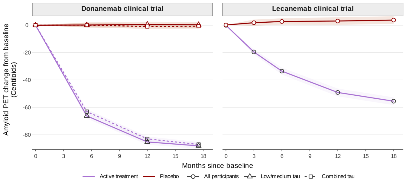
Figure 3.
Alternative study designs improve detectability of a small effect without changing the endpoint. Each panel plots detectability, the proportion of simulated trials in which the intervention effect was detected at the significance threshold, on the y-axis against a swept study-design parameter on the x-axis. Rows correspond to three study designs: two-arm between-individual (top), within-individual split-body (middle), and multi-outcome between-individual (bottom). Columns correspond to the parameter varied: sample size (n, 50–200; left), number of measurement occasions (3–8; middle), and follow-up duration (2–8 years; right). When not being varied, parameters were held at their default values (, three measurements over a two-year follow-up). Within each panel, points represent detectability estimates from individual simulation conditions and lines show the smoothed trend across parameter values. Colors indicate the analysis strategy applied within each design. The horizontal dashed line marks the 0.8 detectability threshold. Each design–analysis combination was simulated in 1000 independent trials. The intervention was modeled as a small reduction in the rate of decline () of a functional measure (handgrip strength), calibrated so that the expected treatment–control difference after two years corresponded to Cohen’s , with within-individual variability set to kg.
Figure 3.
Alternative study designs improve detectability of a small effect without changing the endpoint. Each panel plots detectability, the proportion of simulated trials in which the intervention effect was detected at the significance threshold, on the y-axis against a swept study-design parameter on the x-axis. Rows correspond to three study designs: two-arm between-individual (top), within-individual split-body (middle), and multi-outcome between-individual (bottom). Columns correspond to the parameter varied: sample size (n, 50–200; left), number of measurement occasions (3–8; middle), and follow-up duration (2–8 years; right). When not being varied, parameters were held at their default values (, three measurements over a two-year follow-up). Within each panel, points represent detectability estimates from individual simulation conditions and lines show the smoothed trend across parameter values. Colors indicate the analysis strategy applied within each design. The horizontal dashed line marks the 0.8 detectability threshold. Each design–analysis combination was simulated in 1000 independent trials. The intervention was modeled as a small reduction in the rate of decline () of a functional measure (handgrip strength), calibrated so that the expected treatment–control difference after two years corresponded to Cohen’s , with within-individual variability set to kg.
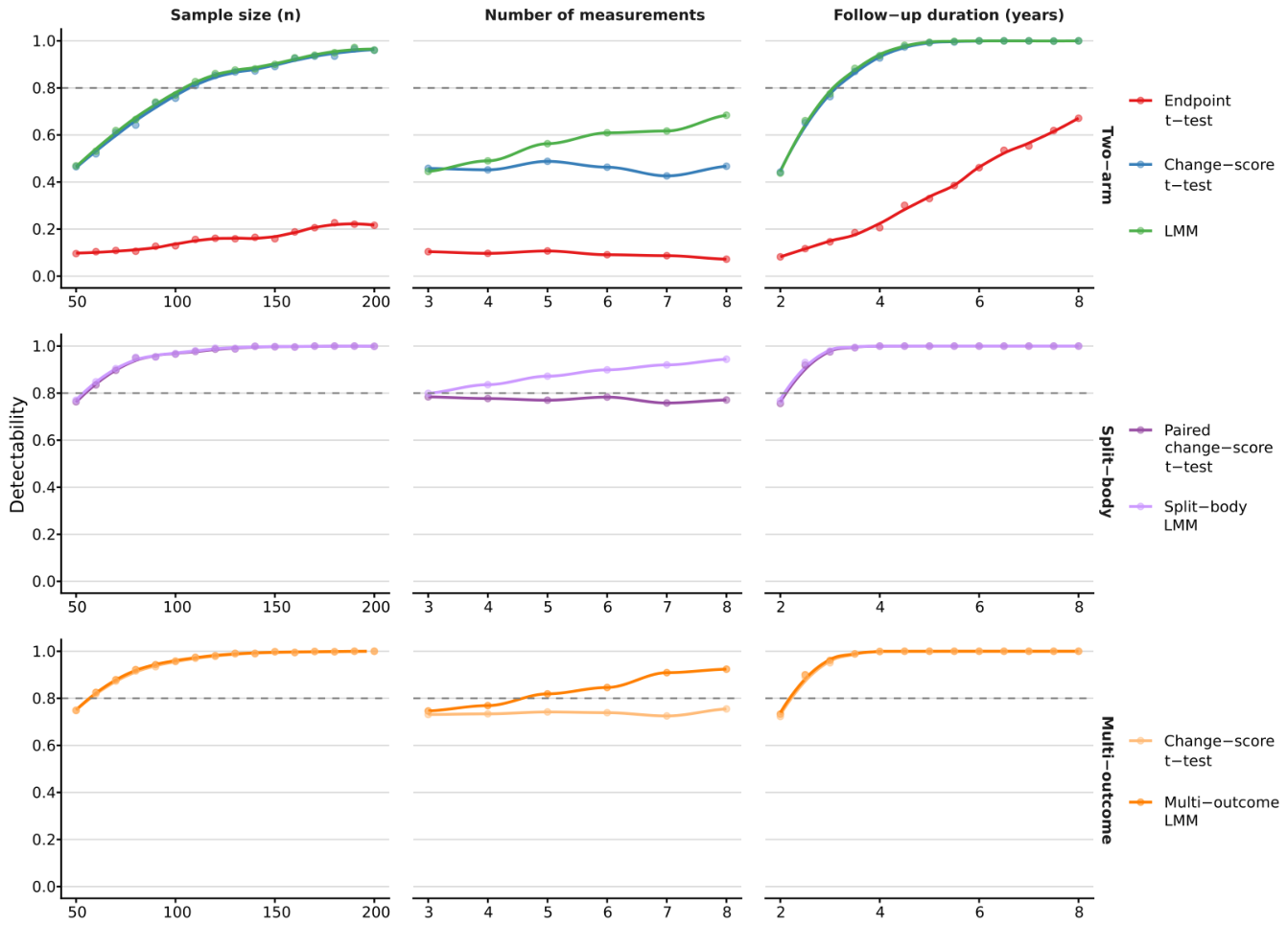
| 1 | Throughout this article, "molecular measures" is used as a broad label for abundance measures of cellular components (e.g. transcripts, proteins, lipids, and metabolites) and their chemical modifications, such as DNA methylation and protein post-translational modification, as well as the statistical composites commonly derived from these features. |
| 2 | Composite measures in gerontology appear under various labels such as "biological age clocks" and "functional" or "healthspan metrics". Some are constructed entirely from molecular features, such as DNA methylation or transcriptomic measures; others combine molecular with non-molecular features, while some contain no molecular measurements at all. |
| 3 | Another key practical utility of a validated model is effective intervention. Since every intervention comes at a cost, understanding the generative process of a system sufficiently well before intervening can help anticipate the consequences and trade-offs involved. |
| 4 | Other factors contributing to the proliferation of these metrics include declining assay costs, increasing accessibility, and the expanding range of measurable molecular features [1-a], and the presumption that molecular measures generalize more readily across species, allowing the same measures to be used in preclinical and human studies and potentially improving translation to humans [5-e]. Their novelty may also play a role, as it aligns well with academic incentives. |
| 5 | This assumption appears in somewhat different forms depending on the endpoint. It is stated most explicitly for outcomes such as lifespan, mortality, and disease incidence, where the event of interest may itself take years to occur and long follow-up therefore appears unavoidable[7-a]. For functional measures the argument is less direct[7-b]. These can be measured at any time, but their age-associated deterioration is treated as gradual, so that over short intervals the expected change is assumed to be small relative to within- and between-individual variation. Detecting it is then taken to require longer follow-up, larger samples, or both. The article focuses on functional measures for two reasons. First, they offer more intuitive examples for the study designs discussed below. Second, the long-standing debate over the inadequacy of lifespan and mortality has itself motivated a growing emphasis on them. The arguments developed below, particularly those concerning surrogate validity under A2, are not specific to functional endpoints and apply equally to lifespan, mortality, or disease incidence |
| 6 | In practice, investigators aim to construct and validate generative models. A validated generative model is essential for effective intervention. It helps anticipate the consequences and trade-offs involved, as every intervention comes at a cost. In general, models are initially formulated as statistical descriptions and are iteratively refined toward generative representations. A model is proposed and predictions are derived from it. Interventions are then used to test whether modifying variables produces outcomes consistent with those predictions. When predictions fail, the model is revised or replaced. |
| 7 | It is important to note that the relationship between x and t considered here is a statistical one. That is, the observed association between the variable and time does not by itself specify the generative processes responsible for that pattern. Multiple distinct generative mechanisms may produce the same statistical relationship between x and t
|
| 8 | Hypothetical scenarios are used throughout the article because simplified, and sometimes extreme, cases can make the logical implications of an argument clearer |
| 9 | An alternative interpretation is that amyloid burden had approached a plateau by this stage [14]. This does not affect the comparison. Whether produces slow accumulation or a plateau, the rapid reduction under occurs on a markedly different time scale. |
| 10 | Larger samples improve the ability to detect small differences between groups, while longer follow-up allows the trajectories under and to diverge further. |
| 11 | In practice, investigators aim to construct and validate generative models. A validated generative model is essential for effective intervention. It helps anticipate the consequences and trade-offs involved, as every intervention comes at a cost. In general, models are initially formulated as statistical descriptions and are iteratively refined toward generative representations. A model is proposed and predictions are derived from it. Interventions are then used to test whether modifying variables produces outcomes consistent with those predictions. When predictions fail, the model is revised or replaced. |
| 12 | This value is larger because the residual captures more than short-term measurement variation. It also includes longer-term within-individual deviations from the assumed trajectory and other variation not explained by the model |
| 13 | Uses only the final measurement from each individual. It compares mean handgrip strength between the treatment and control groups at the end of follow-up. Baseline handgrip is not used, so pre-existing differences between individuals are not accounted for. |
| 14 | Uses only the first and final handgrip measurements. For each individual, a change score is calculated as the difference between these two measurements. The test then compares the mean change score between the treatment and control groups. This removes pre-existing differences in handgrip between individuals from the comparison. However, it reduces two measurements to a single change score, does not model their measurement variability separately, and ignores any intermediate follow-up measurements |
| 15 | Uses all handgrip measurements collected during follow-up. Using these measurements, it estimates the rate of change in handgrip for each individual over time. It then tests whether the average rate of change differs between the treatment and control groups. This makes use of intermediate measurements rather than only the first and last. It also accounts for repeated measurements coming from the same individual |
| 16 | Uses the first and final handgrip measurements from both hands. For each individual, the change from baseline is calculated separately for the treated and untreated hand. These two change scores are then compared within the same individual using a paired t-test. The test asks whether, on average, the treated hand changed more than the untreated hand. Because each individual serves as their own control, stable differences between individuals have less influence on the comparison. However, the analysis reduces four measurements to two change scores and does not model the variability of the individual measurements separately. It also ignores any intermediate follow-up measurements |
| 17 | Uses the first and final handgrip measurements from both hands. For each individual, the change from baseline is calculated separately for the dominant and non-dominant hand. These two change scores are then averaged to give a single overall change score for that individual. The mean overall change is then compared between the treatment and control groups. Averaging across both hands reduces the influence of variation specific to either hand. However, the analysis still reduces the repeated measurements to a single change score and ignores any intermediate follow-up measurements |
| 18 | Strictly, the primary measure () is not always the final thing we care about. It is usually measured because it helps answer a practical question, denoted here by (y). For example, we may care whether an intervention produces enough benefit to justify approval, and use a change in () to make that decision. A surrogate is useful if replacing () with the surrogate leads to the same conclusion about (y). Throughout this article, () and (y) are treated as effectively interchangeable for simplicity, because the primary measure is usually chosen precisely because it is closely tied to the objective. This need not always be true. A surrogate could predict () well but still fail to answer the question represented by (y), or it could be useful for (y) without closely reproducing (). |
| 19 | A third defense sometimes invoked shifts the objective from the individual to the population level. First, this is a different objective rather than a response to whether the intervention is meaningful for the individual. Second, the argument is structurally tautological. Almost any small per-individual effect, when multiplied across a sufficiently large population, yields a large aggregate number. If population-scale aggregation is the relevant criterion, then an intervention with a larger per-individual effect would, across the same population, produce an even larger aggregate benefit. The argument therefore does not favor small-effect interventions specifically. It favors whichever intervention has the larger per-individual effect. Finally, population-level projections are typically derived from models whose outputs depend heavily on their assumptions, many of which simplify the underlying biological, behavioral, and demographic processes |
| 20 | A related consideration for interventions whose benefits lie far in the future is real-world adherence. Willingness to sustain an intervention tends to decline as the gap between action and perceived benefit widens. This is not specific to gerontology. Smoking provides one example. Its long-term health effects are substantial and well established, yet cessation rates remain modest even among individuals aware of the risks. Exercise and dietary modification provide similar examples. Both have well-established benefits, yet sustained adherence remains low. Addiction, palatability, and other factors also contribute, but the point here concerns the temporal structure of the benefit. Both the cost of an intervention and the tangibility of its benefit affect uptake and sustained use. Small-effect interventions requiring prolonged exposure before any perceptible benefit emerges are unfavorable on both dimensions |
| 21 | The same considerations apply reflexively here. As a self-interested amateur working on these questions, the time available to me is finite. Under these constraints, directing limited resources toward interventions expected to have small effects, and whose confirmation may not arrive within a timeframe I am likely to witness, is not a defensible personal allocation. This is not an argument against others pursuing such work, whose circumstances, incentives, or objectives may differ |
| 22 | This point is related to the broader problem of intervention dependence. The same nominal variable may have different consequences depending on the intervention used to modify it. A related discussion appears in the literature on BMI and intervention-dependent causal effects, as well as in [4]. The point is noted here only to delimit the issue; it is not the main focus of the present discussion |
| 23 | Those familiar with "Mendelian randomization" methods may recognize a close analogue to . One of its key assumptions is the exclusion restriction, which requires that the genetic instrument affect the outcome only through the exposure of interest, with no alternative paths linking the instrument to the outcome. The extensive debates over this assumption reflect how difficult it is both to establish that no relevant alternative paths exist and to determine when violations are large enough to undermine the resulting conclusions. |
| 24 | This is consistent with the earlier discussion of provisional approval. Under current regulatory frameworks, endpoints reasonably likely to predict clinical benefit can support conditional approval, but this does not make them equivalent to the primary clinical outcome. Confirmation still requires measuring the clinical endpoint the surrogate was intended to stand in for |
| 25 | This assumes no other protein structure can emit at the same wavelength. In practice this is unlikely, it is a hypothetical to make the example intuitive |
| 26 | A familiar illustration comes from gene-set analyses routinely applied to high-throughput molecular data. Substantially different lists of individual genes can nevertheless "enrich" the same higher-level "biological theme". Historically, however, these methods were not developed explicitly to address biological redundancy or degeneracy. Their stated motivations were largely practical. First, combining small but coordinated changes across many genes could provide greater statistical power than testing each gene separately [24]. Second, simplifying analyses by reducing the large number of measures to a smaller and more manageable set [25-a-b][26]. Third, this was also hoped to help "extract biological meaning" from otherwise difficult-to-interpret lists of genes [25-c][27–30]. Even when poor agreement between gene-level results was recognized, it was treated mainly as a limitation of gene-by-gene analysis rather than as evidence of degeneracy in the underlying biological system [31][30-b]. |
| 27 | The terms "redundancy" and "degeneracy" are related but distinct, and the difference bears on the argument. "Redundancy" is used here in the strict sense of identical duplication: multiple copies of the same component performing the same function, as with duplicated genes [21]. "Degeneracy" refers to a kind of functional redundancy without structural identity — different components or routes that can perform a similar function under some conditions while differing under others. The distinction is not as clean as the labels suggest. "Identity" is continuous rather than binary. The labels mark regions of a spectrum rather than discrete categories. Both arrangements share two consequences. The first is resistance to insult: whether through identical copies or dissimilar routes, the presence of more than one element capable of sustaining a function makes that function harder to abolish — by mutation, by targeted attack, or by the loss or damage of any single component. The second, and the more far-reaching, is evolvability. When a function is held by more than one element, no single element bears the full selective burden of maintaining it. One copy or route is thereby freed to vary — to drift, accumulate change, and potentially take on a new role — while another continues to cover the original function, so that novelty can be explored without the existing capability being lost. The implications nonetheless also differ in an informative way. Strictly redundant elements, being identical, share their failure modes: a perturbation that disables one — a toxin, an inhibitor, a condition the mechanism cannot tolerate — disables the others in the same way. Degenerate elements, being structurally dissimilar, might not share failure modes; a perturbation that defeats one route need not defeat the others. The trade-off runs the other way too: redundancy may be easier to manage, since identical elements can be governed by the same control, whereas degenerate routes, being dissimilar, may each require their own. This is itself an instance of the point at issue — every structural arrangement carries its own trade-offs and properties, and which is favored is dictated by the constraints imposed on the system. |
| 28 | This is a general principle of system design, sometimes termed the "paradox of robustness" — though it ceases to seem paradoxical once considered. The example commonly used to illustrate it is data storage. A single hard drive holding valuable data must be built to high reliability, since its failure is catastrophic and its errors corrupt the data irrecoverably — and such reliability is expensive. Once data is instead distributed redundantly across an array of drives, with a higher-level mechanism reconstructing the contents of any drive that fails, the failure of an individual drive is no longer catastrophic. The reliability demanded of each drive accordingly falls, and the economically favored design shifts toward cheaper, higher-failure-rate components whose errors are absorbed by the system. The same logic operates wherever reliability is secured at the system level: error correction at the top relaxes the performance required at the bottom, and components are permitted — and over evolutionary time, expected — to drift toward sloppier, lower-cost states |
| 29 | In gerontology, molecular imperfection is sometimes invoked as an argument for the inevitability of system-level deterioration. The reasoning is that stochastic molecular behavior and low but non-zero error rates amount to an entropic process that cannot be escaped. However, system-level organization can maintain reliable function despite noisy and imperfect components. Biological systems can tolerate, segregate, repair, replace, or eliminate damaged components, and many such mechanisms are already known. Asymmetric cell division provides a simple example, where damaged material can be preferentially segregated into one daughter cell. |
| 30 | Especially those measures that aim to represent "biological age" or overall "functional state" [34][3-a][4] |
| 31 | This account necessarily compresses a century of observations, debates, and revisions into a few sentences |
| 32 | Effects were not uniform in magnitude or timing across compounds, but the direction — reduced Aβ, no cognitive benefit — was consistent across all five. |
| 33 | Solanezumab was designed to bind soluble, monomeric Aβ rather than aggregated plaque, and accordingly showed no change in plaque burden on PET. It did engage its intended target: plasma Aβ rose substantially and was sustained throughout treatment, consistent with the antibody binding and redistributing the peptide from brain to periphery. Despite this confirmed engagement, there was no effect on cognition. |
| 34 | The trials were prospectively described as identically designed. In practice, they differed in timing and dosing: ENGAGE began a month before EMERGE, and two mid-trial protocol amendments intended to raise more patients to the full target dose affected a larger share of EMERGE’s participants, since EMERGE enrolled more patients after the amendments took effect. The authors invoke this difference to explain why ENGAGE failed where EMERGE succeeded. But the biomarker data sit uneasily with this account: amyloid PET reduction and plasma p-tau reduction were similar in magnitude between the two trials at week 78 — amyloid clearance was only about 16.5% smaller in ENGAGE than in EMERGE — while the clinical outcomes were not merely smaller in ENGAGE but null, and in the high-dose arm numerically worse than the low-dose arm on the primary endpoint. A dosing shortfall of that size is not an obvious explanation for a difference that large. Whether the true cause was the dosing difference, chance, or something else entirely is disputed. |
| 35 | Symptomatic drugs (e.g. cholinesterase inhibitors) treat the effects of neuronal loss without altering its underlying cause or rate. That amyloid clearance produces a benefit no larger than these is notable precisely because it targets the purported cause rather than the symptom. |
| 36 | Framing the problem this way is deliberate. The difficulties that follow are the familiar difficulties of model construction. The earlier discussion of constraints can be read in the same terms. |
| 37 | The yeast case is useful because it grants the measure-more strategy unusually favorable conditions. The system is a single cell, can be systematically perturbed, the context can be fixed, and the endpoint is cheap, direct, and reached in a day. Gerontology removes each of these advantages. The object is a multicellular organism, so the route from molecular state to function can differ across tissues, individuals, and time. The context is neither fixed nor fully observable. The system cannot be exhaustively perturbed. The endpoint is slow and costly to observe, while many molecular measurements are invasive or destructive, limiting the trajectories that can be collected from the same individual over time. |
| 38 | The appeal of such theories is that, if correct, they simplify both measurement and intervention. They imply a relatively centralized structure in which much of the downstream deterioration is mediated through one or a few upstream factors. Measuring those factors could therefore provide an accessible summary of a much broader downstream state. The same structure would also simplify intervention, because altering the relevant factors could in principle modify many downstream effects at once. |
| 39 | Whether a trait is “genetically determined” is easily conflated across distinct claims [54-a] [55-a] [56-a]. Genes and their products are necessary for the development and maintenance of essentially every organismal trait, but this does not imply that naturally occurring sequence variation in any gene required for the trait will explain variation in the trait itself. A similar conflation is common in gerontology, where a gene knockout that increases or decreases lifespan is sometimes taken to imply that naturally occurring variants in that gene would explain differences in lifespan. Knocking out a structural component may collapse the system without revealing how differences arise within an intact system. Necessity under disruption is therefore not equivalent to explanatory or predictive importance under “natural” variation [57-a] [57-b]. |
| 40 | The looseness of the terms “complex trait” and “complex disease” warrants caution. They are used broadly in the literature to denote traits whose inheritance departs from simple Mendelian patterns, but the resulting category is neither sharply defined nor biologically uniform. It includes metabolic, autoimmune, and psychiatric disorders, as well as continuously distributed traits such as height and blood pressure [58-a]. No single genetic architecture should therefore be expected across it: the number of associated loci, the magnitude and distribution of their effects, and their dependence on environmental and population context vary substantially both within and between these groups. The terminology is retained here because it is conventional in the relevant literature, though it is arguably ill-defined and of limited conceptual precision for the kinds of distinctions and arguments made in the present discussion [58-b]. |
| 41 | “Categorical” and “quantitative” are not separate classes of traits. The categorizability of a measure is a matter of degree and resolution. Any measure can be divided into categories; the question is how readily this can be done. The labels reflect agreement among categorizers: give the same distribution to different observers, ask them to divide it into groups, and compare their answers. “Categorical” traits produce higher consensus. In statistical terms, this relates to modality. A clearly bimodal distribution invites a similar split; a single mode does not. “Quantitative” usually refers to unimodal traits, where individuals differ by degree and no "clear" boundary separates them into a small number of types. |
| 42 | Other explanations were also proposed, including locus and allelic heterogeneity, environmental confounding, and imperfect [58-c] or convergent phenotype definitions in which similar clinical outcomes arise from different underlying causes. These issues remained challenges for subsequent association studies |
| 43 | The direction of inference warrants emphasis. The infinitesimal model showed how continuous variation could arise under assumptions of numerous small, approximately additive genetic effects and environmental variation. Under these assumptions, it can produce an approximately Gaussian distribution resembling that observed for many quantitative traits. The resemblance does not, however, establish that this is the process that generated the distribution. The same or similar observed distribution may arise from different underlying mechanisms. Observing approximate normality is therefore compatible with the infinitesimal model, but does not by itself confirm its assumptions or identify the underlying causal structure. |
| 44 | What exactly the CDCV hypothesis predicted remains contested [59-d], partly because its early formulations made few firm quantitative claims about how common risk alleles should be, how many loci should contribute, how large their effects should be, or how much disease risk they should collectively explain. Interpretations ranged from a narrow claim about a “simple allelic spectrum” at particular loci to broader claims about the relationship between disease prevalence and the genome-wide frequency and abundance of susceptibility alleles |
| 45 | Proponents of the CDCV hypothesis also drew support from a small number of then-prominent reports in which common alleles, most notably APOE ε4, were associated with appreciable disease risk [60-d]. Although these examples were consistent with the hypothesis, other disorders, particularly Mendelian ones, showed extensive allelic heterogeneity, with many independently arising rare mutations and no predominant allele [60-e]. This contrast was attributed to stronger purifying selection against variants causing severe, early-onset disease. Examples could therefore be marshalled on either side, while the small and possibly biased sample of characterized loci provided only a thin basis for a general claim about allelic architecture. |
| 46 | The optimism surrounding the CDCV hypothesis was not universal. Around the same time, Pritchard used a related population-genetic modelling approach but reached a less favourable conclusion, emphasizing that allelic heterogeneity could leave no single susceptibility variant at high frequency and substantially reduce the power of association mapping [68-ab] [60-f]. The contrast with Reich and Lander arose less from radically different numerical predictions than from differences in assumptions, emphasis, and interpretation. |
| 47 | What is commonly called the reference genome is a consensus representation. This has consequences for the notion of a genetic “background”. Human populations contain substantially divergent haplotypes. The shift from a single consensus to pangenome references - graphs assembled from many individual haplotypes - was a direct response to this diversity. The combinations of these common alternatives generate a large number of genomic backgrounds. This problem does not disappear within an individual. Somatic mutations arising during development and later life generate genetically distinct clonal lineages, so different cells within the same organism need not share an identical genome [57-d]. The background against which a variant acts therefore varies both between individuals and among cells within the same body. |
| 48 | Further complications include maternal effects [80], parent-of-origin effects, and mito-nuclear interactions [81], to name a few. |
| 49 | Any model is constructed at a particular level of resolution, and the appropriate level depends on the objective. A single system, such as the human body, can be modeled in radically different ways depending on the goal. Designing an elevator may only require coarse descriptors like average height and weight. Modifying a gene might demand a finer resolution, where those same descriptors might be of limited utility. There is no level at which the system is described “as it really is”, only levels that are adequate or inadequate to a given question. This is why no measure can be ranked as a better or worse surrogate without first fixing the objective it is meant to serve. |
| 50 | The same principle is intuitive at another scale. To determine whether someone speaks English, one could attempt to infer it from the structure and activity of the brain, or simply ask them a question in English and observe the response. |
| 51 | Senolytics pursue a structurally similar objective [88]. They aim to eliminate a subset of cells from the body in pursuit of long-term health outcomes. Decades of oncology therefore provide an empirical precedent for both the promise of molecular targeting and the conditions under which it is likely to succeed. |
| 52 | Molecular targeting is only one class of oncological intervention. Other successful approaches include surgical resection and radiotherapy for localized disease, as well as cytotoxic chemotherapy. Some cancers are remarkably sensitive to the latter such as testicular germ-cell tumors and low-risk gestational trophoblastic neoplasia. |
| 53 | This classification problem is difficult for several reasons. First, tumor cells originate from the host. They are built from the same molecular repertoire as the rest of the body and depend on much of the same machinery. Second, tumorigenesis is heterogeneous, both within and across individuals. The mutations, pathways, and configurations that produce a tumor cell are not uniform. Many distinct molecular routes can lead to comparable cellular behavior. Third, what is meant by a "tumor cell" is itself worth making explicit. A cell is labeled tumorigenic if, left in place, it would contribute to the formation of a mass capable of harming the individual. This is a behavioral rather than molecular definition, and the same behavior can arise through many configurations, including overactivation of growth-promoting genes, loss of growth-suppressing ones, metabolic rewiring, and evasion of programmed cell death. Mammalian cells are substantially degenerate, and no single molecular component is universally essential to the tumorigenic phenotype. Finally, the intervention itself changes the population being targeted. Any targeting rule imposes selection on the targeted feature. By eliminating cells that satisfy the rule, the intervention enriches for cells that do not. If even a small subpopulation lacks the target through pre-existing heterogeneity, reduced expression, or alternative configurations that achieve the same function, that subpopulation is more likely to survive and expand. |
| 54 | CML lies near one extreme of a broader spectrum. Other successful molecular targets are shared less uniformly, are less uniquely tied to the malignant state, or produce less complete responses when targeted. Examples include PML–RARA in acute promyelocytic leukemia, CD20 in B-cell lymphomas, CD19 in B-cell leukemias and lymphomas, and HER2 in HER2-positive breast cancer. Their effectiveness varies with how consistently the target is present, how strongly the malignant cells depend on it, whether normal cells also express it, and how readily the cancer can escape its loss. |
| 55 | The compound was not yet called imatinib in the 1996 study; that name was adopted later. |
| 56 | CML provides another example of the "more the merrier" approach. One response to resistance is to widen target coverage, either by combining agents or by developing a single agent active against several relevant variants or targets. Ponatinib was designed to inhibit both native and mutant BCR–ABL1, including the T315I variant that confers resistance to earlier inhibitors, and also inhibits several other kinases. It restored responses in many heavily pretreated patients, including those with T315I disease. This broader activity, however, came with substantial toxicity. Serious arterial occlusive events emerged after approval. The toxicity was severe enough that the drug was temporarily withdrawn in 2013 and returned only with a boxed warning and a narrowed indication. Broad kinase inhibition has been proposed as one contributor to this toxicity. Ponatinib therefore illustrates a potential trade-off of increasing target coverage. Doing so may reduce some routes to resistance, while also increasing the number of normal processes affected by the intervention. |
| 57 | These cases also illustrate how a common initiating cause need not produce a common molecular cancer state. The same virus or bacterium can give rise to malignancy through different combinations of subsequent cellular changes. |
| 58 | Ferguson (2002)’s review was especially helpful here. It made the objective explicit, laid out the assumptions required for genetic divergence to serve as a species criterion, and examined the different ways reproductive isolation can arise. |
Disclaimer/Publisher’s Note: The statements, opinions and data contained in all publications are solely those of the individual author(s) and contributor(s) and not of MDPI and/or the editor(s). MDPI and/or the editor(s) disclaim responsibility for any injury to people or property resulting from any ideas, methods, instructions or products referred to in the content. |
© 2026 by the authors. Licensee MDPI, Basel, Switzerland. This article is an open access article distributed under the terms and conditions of the Creative Commons Attribution (CC BY) license (http://creativecommons.org/licenses/by/4.0/).
Copyright: This open access article is published under a Creative Commons CC BY 4.0 license, which permit the free download, distribution, and reuse, provided that the author and preprint are cited in any reuse.