

Submitted:
14 September 2026
Posted:
15 September 2026
You are already at the latest version
Abstract
Forest and land fires in Southern Riau, Indonesia, vary seasonally with environmental and landscape conditions. This study evaluated whether separate seasonal models reveal susceptibility patterns not captured by an all-season model and whether preceding environmental change adds predictive information. All-season, dry-season, and rainy-season models were developed from multi-source satellite and geospatial data for 2010–2024 using Logistic Regression, Random Forest, XGBoost, and LightGBM under condition-only and condition-change configurations. Models used a 1:5 fire-to-non-fire ratio, a stratified 70:30 train–test split, and PR-AUC as the primary metric. LightGBM was selected for all periods, with held-out PR-AUC values of 0.921, 0.905, and 0.966, respectively. Historical change improved PR-AUC by 0.008 for all-season and 0.009 for dry-season but decreased it by 0.001 for rainy-season, where condition-only was retained. All-season and dry-season maps were more spatially similar to each other than to the rainy-season map, whose model-derived contributions were led by wind speed, vegetation condition, and peat-related context. Independent 2024 POLRI records showed that 77.60%, 76.79%, and 78.57% of matched incidents fell within High or Very High susceptibility classes. Overall, separate seasonal modelling revealed patterns not fully represented by the all-season model, while the value of preceding environmental change differed among periods.
Keywords:
wildfire susceptibility
; Southern Riau
; seasonal modelling
; machine learning
; remote sensing
; spatial analysis
1. Introduction
Forest and land fires remain a recurrent environmental challenge in Indonesia, particularly across peatland and human-modified landscapes [1,2]. Their occurrence reflects interactions among climatic conditions, vegetation and moisture status, land use, topography, hydrology, and human activity rather than the influence of any single environmental factor [3,4]. Wildfire susceptibility mapping provides a spatial framework for identifying locations where combinations of these conditioning factors are comparatively favourable for fire occurrence and can therefore support the spatial prioritization of monitoring and prevention efforts [4,5].
Fire activity in Indonesia varies substantially within the year and is generally concentrated during drier periods, when reduced rainfall and moisture availability promote vegetation and fuel drying [1,6]. Fire-related susceptibility may nevertheless persist outside the principal dry period because local conditions continue to reflect interactions among meteorological, vegetation, moisture, peatland, land-use, and accessibility factors [2,7]. Representing contrasting environmental periods within a single all-season model may therefore obscure season-specific spatial patterns and predictor relationships [5,7]. Separate seasonal modelling provides a means of evaluating whether the spatial distribution of susceptibility and the contribution structures learned by the models differ among all-season, dry-season, and rainy-season conditions [5,7,8].
Machine-learning and geospatial approaches have increasingly been applied to wildfire susceptibility modelling in Indonesia across local, regional, island, and national scales [8,9,10,11]. Previous studies have shown that predictive performance and influential environmental variables can vary with geographical setting, modelling period, predictor composition, and analytical design [8,10,11]. However, quantitative comparisons of all-season, dry-season, and rainy-season susceptibility patterns remain limited in Southern Riau, particularly with respect to cross-season spatial agreement, persistent and season-specific upper-susceptibility areas, and spatially explicit model-derived contribution patterns [8,11]. Indonesian wildfire studies have also largely emphasized annual, static, or contemporaneous environmental conditions, so the additional predictive value of preceding environmental trajectories remains less explored [8,10]. State–trend approaches provide a framework for integrating current environmental conditions with preceding trajectories, but the predictive value of historical information must be evaluated empirically because its contribution may vary across environmental and modelling contexts [12].
Model interpretation and external validation provide complementary information beyond predictive performance by clarifying how fitted models use environmental predictors and whether mapped susceptibility corresponds spatially with independent fire observations [10,11]. Previous Indonesian studies have used predictor-importance analysis, partial-dependence analysis, SHapley Additive exPlanations (SHAP)-based interpretation, or independent fire observations, but these components have generally been examined separately rather than integrated with quantitative cross-season map comparison, spatial dominant-driver analysis, and interannual susceptibility assessment within a single regional seasonal framework [8,10,11]. Building on previous seasonal and state–trend modelling approaches, this study develops all-season, dry-season, and rainy-season wildfire susceptibility models for Southern Riau using multi-source satellite and geospatial data from 2010–2024 [5,7,12]. Logistic Regression, Random Forest, XGBoost, and LightGBM are compared under condition-only and condition-change predictor configurations, followed by quantitative cross-season spatial comparison, SHAP-based global and spatial interpretation, interannual susceptibility assessment, and external spatial validation using independent 2024 Indonesian National Police (POLRI) fire-incident records [8,9,10,11]. Through this framework, the study evaluates whether preceding environmental trajectories provide season-dependent predictive information and whether separate seasonal models reveal susceptibility patterns and model-derived contribution structures that may be obscured by an all-season representation alone [5,7,12].
2. Materials and Methods
2.1. Study Area
Southern Riau is located in Riau Province, Sumatra, Indonesia [13]. The study area comprises four contiguous regencies—Kuantan Singingi, Indragiri Hulu, Indragiri Hilir, and Pelalawan—with a total administrative area of approximately 40,113 [13]. These regencies were treated as a single regional modelling unit representing contrasting inland, lowland, riverine, agricultural, plantation, coastal, wetland, and peat-influenced environments within the broader Riau landscape [14].
The spatial unit of analysis was a common 500 m grid projected in EPSG:23833, providing a consistent spatial framework for integrating the multi-source predictor datasets (Figure 1). The study area encompasses substantial variation in vegetation, hydrology, land use, topography, peatland occurrence, and human accessibility, providing an appropriate regional setting for evaluating seasonal differences in wildfire susceptibility [14]. The location, administrative extent, and land-cover context of the Southern Riau study area are shown in Figure 2.
2.2. Research Workflow
The methodological workflow was designed to develop, compare, interpret, and externally assess seasonal wildfire susceptibility models for Southern Riau within a consistent spatial and modelling framework (Figure 1). The workflow began with study-area preparation and multi-source data acquisition, followed by product-specific quality control, seasonal temporal filtering, spatial harmonization to the common 500 m grid, missing-value screening, and grid–year–season dataset assembly (Figure 1). Seasonal burned-area response labels were constructed from MODIS MCD64A1 BurnDate, while environmental and landscape predictors were organized into condition-only and condition-change configurations, with the latter incorporating historical environmental trajectories derived exclusively from years preceding the target year [12,15,16].
Predictor screening combined conceptual and redundancy assessment, GeoDetector analysis, and Random Forest-based Recursive Feature Elimination (RF-RFE) before common-sample construction, 1:5 fire-to-non-fire sampling, and a stratified 70:30 train–test split [17,18,19]. Logistic Regression, Random Forest, XGBoost, and LightGBM were subsequently compared using held-out PR-AUC as the primary model-selection criterion, supported by ROC-AUC, precision, recall, F1-score, Brier score, and confusion-matrix components [20,21,22,23,24,25]. The selected models were used to generate 2024 susceptibility maps and interannual susceptibility summaries [5]. Model interpretation was conducted using SHAP-based global and spatial attribution analyses [26,27]. Independent POLRI fire-incident records were subsequently used for presence-only external spatial validation of the final 2024 susceptibility maps (Figure 1).
2.3. Data Sources and Spatial Harmonization
This study integrated satellite, climate, topographic, hydrological, land-use, peatland, plantation, accessibility, and fire-incident datasets. The principal datasets, source products, temporal coverage, and native spatial characteristics are summarized in Table 1. Cloud-based datasets were accessed through Google Earth Engine (GEE), including MODIS MCD64A1 burned area, CHIRPS precipitation, TerraClimate meteorological variables, MODIS vegetation and land-surface products, SRTM topography, and HydroSHEDS [16,28,29,30,31,32,33,34,35]. Administrative boundaries, Rupabumi Indonesia (RBI) road, river, and settlement layers, peat polygons, and independent POLRI fire-incident records were prepared through local geospatial processing. Annual oil-palm land-cover rasters were obtained from MapBiomas Indonesia Collection 4.1 [36]. The landscape layers represented land-use, accessibility, and peatland contexts relevant to fire susceptibility in Riau [14,37,38].
All raster and vector datasets were clipped to the Southern Riau study area and harmonized to the common 500 m modelling grid in EPSG:23833, yielding 159,703 retained grid cells after clipping (Figure 1). Spatial harmonization was data-type specific. MOD13Q1 NDVI and SRTM-derived continuous variables were aggregated using mean reduction, categorical land cover was aligned using a class-preserving nearest-neighbour operation, and annual binary oil-palm classifications were aggregated to fractional coverage [30,34,39]. Road, river, and settlement vectors were rasterized before grid-based Euclidean proximity calculation, whereas peat polygons were converted to a binary peat mask following the implemented spatial-processing workflow and the broader environmental representation used in Riau fire-susceptibility studies [14].
Product-specific quality control, masking, and scaling were applied where required before seasonal aggregation and dataset assembly [30,31,32,33]. MOD13Q1 NDVI retained observations with SummaryQA values of 0 or 1 and applied the 0.0001 scale factor [30]. MOD09A1 surface reflectance was screened using the State QA layer for cloud state, cloud shadow, and aerosol condition, and reflectance values were restricted to the documented valid range before NDII calculation [31,40]. MOD11A2 daytime LST retained observations with mandatory QA bits equal to 00 and estimated LST error not exceeding 2 K, while MOD15A2H LAI was screened using FparLai_QC and converted using the corresponding product scale factor [32,33]. TerraClimate variables were converted to their physical units before seasonal aggregation, and relative humidity was derived from vapour pressure and temperature [29,41]. CHIRPS Pentad precipitation was accumulated within each seasonal modelling window [28]. TVDI was derived from the seasonal NDVI–LST feature space using wet- and dry-edge estimation and was interpreted as a vegetation–thermal dryness indicator rather than as an independent source product [42].
The harmonization procedure standardized the coordinate reference system, pixel size, spatial extent, grid origin, affine transform, and raster structure across the predictor layers (Figure 1). Alignment to the 500 m analytical grid did not create genuine 500 m environmental information from coarser-resolution products; CHIRPS, TerraClimate, and MODIS LST retained effective information scales close to their native resolutions of approximately 5.6 km, 4.6 km, and 1 km, respectively [28,29,32]. The harmonized layers were therefore treated as spatially aligned multi-source inputs rather than statistically downscaled or spatially sharpened products [28,29,32].
Source-specific NoData, sentinel, non-finite, and otherwise invalid values were treated as missing before final dataset assembly (Figure 1). Records were retained only when the response and all predictors required by the active configuration were valid; no statistical imputation was applied in the final workflow (Figure 1). Condition-only and condition-change datasets were screened separately for completeness before construction of the matched common samples used for model comparison (Figure 1).
Local data processing, feature screening, machine-learning analysis, model evaluation, and model interpretation were conducted in Python 3.11.15 using scikit-learn 1.8.0, XGBoost 3.1.3, LightGBM 4.6.0, and SHAP 0.51.0. Cloud-based geospatial data access and preprocessing were conducted using Google Earth Engine (GEE).
2.4. Seasonal Response and Predictor Construction
Three modelling periods were defined and analysed independently: all-season, dry-season, and rainy-season. Regional BMKG information indicates that Riau experiences two dry-season and two rainy-season periods within the year [43]. Seasonal wildfire modelling has likewise been used to represent contrasting fire environments that may exhibit different spatial and environmental relationships [8]. For analytical consistency across the 2010–2024 study period, fixed month windows were therefore adopted as operational modelling periods rather than as year-specific estimates of seasonal onset or cessation. The same analytical windows were applied consistently to response-label construction, aggregation of dynamic predictors, calculation of historical trends, and generation of the final 2024 susceptibility maps (Figure 1).
The all-season period was operationally defined as January–December of the target year, whereas the dry-season period covered May–October of the target year. The rainy-season period followed a cross-year definition extending from November of the preceding year through April of the target year. Accordingly, the rainy-season period associated with target year 2024 covered November 2023–April 2024.
Because the rainy-season window crosses calendar years, the dry- and rainy-season observations associated with a given target year do not constitute an exact temporal partition of the corresponding all-season calendar-year observations [5,8]. Each modelling period was therefore treated as an independent analytical dataset with its own response labels, predictor summaries, feature-screening results, trained models, and susceptibility outputs [5,7].
Seasonal response labels were constructed from the MODIS MCD64A1 Burned Area product [15,16]. The BurnDate layer records the approximate day of burning within each monthly observation and was used to assign detected burned areas to the corresponding modelling window [15]. The response therefore represented satellite-detected burned-area occurrence at the 500 m grid scale rather than a complete field inventory of all fire incidents [15,16].
For each grid cell, target year, and modelling period, a fire label of 1 was assigned when at least one BurnDate value greater than 0 occurred within the corresponding temporal window [15]. Cells without a detected BurnDate were initially treated as potential non-fire observations rather than confirmed fire absences because satellite burned-area products remain subject to omission and commission errors [16].
Before the negative class was finalized, a 1 km exclusion buffer was applied around detected burned cells to reduce ambiguity associated with mixed pixels, positional uncertainty, burn-edge effects, and environmental conditions immediately adjacent to detected burned areas [16]. Remaining eligible cells outside both detected burned areas and the exclusion buffer were assigned an operational non-fire label of 0 under the implemented response-construction procedure (Figure 1).
Predictors were organized into condition-only and condition-change configurations following the distinction between current environmental state and preceding environmental trajectories [12]. The condition-only configuration represented environmental and landscape conditions associated with the target modelling period, including precipitation, air temperature, relative humidity, wind speed, soil moisture, vegetation condition, land-surface temperature, land cover, topography, hydrological setting, peatland context, oil-palm coverage, and accessibility-related variables [3,4].
The condition-change configuration incorporated historical environmental trajectories calculated exclusively from years preceding the target year [12]. Candidate historical indicators included trends in NDVI, NDII, soil moisture, and TVDI, subject to data availability and subsequent feature screening [12]. For each target year t, historical trends were calculated over the preceding 10-year interval, to , thereby excluding the target year and preventing temporal leakage [12]. The 10-year interval was selected after sensitivity testing of 5-, 8-, 10-, 12-, and 15-year alternatives under the implemented historical-window comparison (Figure 1).
Historical change was summarized using Sen’s slope, a non-parametric estimator of monotonic trend magnitude [44]. For a time series , Sen’s slope was calculated as
where and denote observations at time steps i and j, respectively, and represents the median rate of change over the historical window [44]. The Mann–Kendall statistic was retained as supporting information on trend direction and monotonicity rather than as a model predictor [45,46,47]. Following predictor screening, NDII trend and soil-moisture trend were retained as the historical components of the final condition-change predictor sets, whereas NDVI trend was not retained after screening and TVDI trend was not retained where it was evaluated (Figure 1). Rainy-season TVDI trend was not included in the active historical-predictor pool because its historical coverage was insufficient under the verified data-completeness criteria (Figure 1).
2.5. Predictor Screening and Feature Selection
Predictor screening and selection were conducted before model comparison using a six-stage workflow applied separately to each modelling period and predictor configuration [17,18,48]. The workflow comprised (1) conceptual filtering, (2) Spearman correlation and Variance Inflation Factor (VIF) screening, (3) GeoDetector factor and interaction analysis, (4) Random Forest-based Recursive Feature Elimination (RF-RFE), (5) family-based redundancy review, and (6) stability-based final predictor-set construction [17,18,49,50].
The conceptual filter evaluated each candidate predictor according to its relevance to wildfire susceptibility, temporal availability, spatial coverage, suitability for the Southern Riau landscape, interpretability, and potential risk of target leakage [3,51]. Administrative identifiers, spatial coordinates, target year, modelling-period labels, and other metadata used solely for data management and mapping were excluded from model fitting to prevent non-environmental identifiers from entering the predictor set (Figure 1).
Spearman rank correlation and VIF were subsequently used to diagnose pairwise redundancy and multivariable collinearity among candidate predictors [49,50]. Predictor pairs with were flagged for review rather than removed automatically, allowing statistical dependence to be considered together with physical meaning and temporal role [49,50]. VIF values below 5 were treated as acceptable, values from 5 to less than 10 prompted review, and values of 10 or greater prompted strong review under the study-specific screening framework [50]. Retention decisions also considered data quality, conceptual relevance, and evidence from subsequent screening stages rather than relying on a single numerical threshold [50,52]. The highly redundant air-temperature family was consequently reduced by retaining maximum temperature as the representative atmospheric-temperature predictor under the study-specific screening results (Figure 1).
GeoDetector was then used to evaluate spatial explanatory structure [17]. The Factor Detector ranked individual predictors using the q-statistic, whereas the Interaction Detector assessed whether pairs of predictors exhibited stronger spatial explanatory power when considered jointly [17]. The q-statistic was calculated as
where h denotes a stratum of the explanatory variable, L is the total number of strata, and denote the number of observations and variance of the response within stratum h, respectively, and N and denote the corresponding quantities for the entire dataset [17]. The q-statistic ranges from 0 to 1, with larger values indicating stronger spatial explanatory power [17]. Continuous predictors were discretized before GeoDetector analysis, and multiple discretization methods and class numbers were evaluated following optimized GeoDetector applications [17,48]. GeoDetector results were treated as spatial explanatory evidence rather than as measures of predictive performance or causal effects [17,53].
RF-RFE was used as the predictive feature-selection stage [18]. Random Forest served as the base learner, while Recursive Feature Elimination iteratively evaluated reduced predictor subsets [18,20]. For categorical predictors such as land cover, dummy-variable importances were aggregated back to the corresponding source variable before predictor ranking under the implemented feature-selection workflow (Figure 1). PR-AUC, operationalized as Average Precision, was used as the principal RF-RFE performance metric, with ROC-AUC and F1-score used as supporting measures [23,24]. RF-RFE was used only for predictor selection and did not determine the final machine-learning algorithm [18].
Finally, predictors representing closely related environmental processes were reviewed as variable families to reduce unnecessary redundancy while preserving complementary environmental information [3,52]. Current-condition variables and their corresponding historical trends were not treated as automatically redundant because they represent different temporal dimensions [12]. Final predictor sets were established by jointly considering conceptual relevance, correlation and VIF diagnostics, GeoDetector evidence, RF-RFE performance, family-level redundancy, data coverage, physical interpretability, and stability across screening stages [17,18,50]. No single statistic was used as an automatic inclusion or exclusion criterion [17,50]. Final predictor sets were constructed independently for each modelling period and for the condition-only and condition-change configurations to preserve season- and configuration-specific information [8,12].
2.6. Sampling Design and Machine-Learning Models
To ensure a controlled comparison between the condition-only and condition-change configurations, modelling was performed using matched common samples within each seasonal period (Figure 1). After condition-change completeness filtering, the corresponding condition-only datasets were restricted to the same grid-cell and target-year records (Figure 1). Consequently, both predictor configurations within a modelling period used identical observations, response labels, sampled records, and train–test memberships, preventing performance differences from being attributable to differences in the observation sets [12].
The resulting common-sample datasets remained strongly imbalanced, consistent with the rare-event structure commonly encountered in wildfire susceptibility data [19,23]. Fire observations represented 0.3247% of the all-season dataset, 0.2219% of the dry-season dataset, and 0.1587% of the rainy-season dataset, corresponding to approximate fire-to-non-fire ratios of 1:307, 1:450, and 1:629, respectively (Table 2). All fire observations were retained, whereas operational non-fire observations were randomly sampled without replacement at five times the number of fire observations to reduce extreme class imbalance while preserving all available positive observations [19]. Non-fire sampling was conducted before the train–test split using a fixed random seed of 42 to ensure reproducibility of the implemented sampling procedure (Figure 1).
The resulting sampled datasets contained 6,514 fire and 32,570 non-fire observations for all-season, 3,428 fire and 17,140 non-fire observations for dry-season, and 1,665 fire and 8,325 non-fire observations for rainy-season (Table 2). Each sampled dataset was divided into 70% training and 30% held-out subsets using stratified random splitting with the same random seed, preserving the sampled positive-class proportion across the two subsets [19]. No additional resampling or class weighting was applied after the 1:5 non-fire sampling [19].
Four machine-learning algorithms were evaluated: Logistic Regression, Random Forest, XGBoost, and LightGBM [20,21,22,54]. Logistic Regression served as a regularized linear baseline, Random Forest represented a bagging-based tree ensemble, and XGBoost and LightGBM represented gradient-boosting tree ensembles [20,21,22,54]. The complete model comparison therefore comprised 24 runs: three modelling periods × two predictor configurations × four algorithms (Figure 1). Each model was fitted once to the complete 70% training subset using fixed algorithm-specific hyperparameters that were held constant across modelling periods and predictor configurations (Table 3). No cross-validation-based hyperparameter search was conducted in the final comparison; the analysis therefore focused on algorithm and predictor-configuration differences under fixed modelling settings (Table 3). The final sampled datasets and corresponding train–test composition are summarized in Table 2.
The fixed hyperparameters used for the four machine-learning algorithms are listed in Table 3.
2.7. Model Evaluation and Selection
All 24 candidate model runs were evaluated on the corresponding 30% held-out subsets using complementary ranking, discrimination, threshold-based, and probabilistic metrics [23,24,25]. The held-out observations were not used to estimate model parameters, but their performance metrics were used to compare candidate configurations and select the final model for each modelling period (Figure 1). The resulting values were therefore interpreted as held-out comparative performance rather than fully independent post-selection estimates because the same held-out subsets contributed to candidate ranking and final model selection (Figure 1).
PR-AUC, operationalized as Average Precision, was used as the primary model-selection metric because fire remained the minority class even after 1:5 sampling [23]. Average Precision summarizes precision–recall performance across ranked predictions while emphasizing performance for the positive class [23]. Because precision–recall performance depends on the prevalence of the positive class in the evaluated sample, PR-AUC was interpreted within the adopted 1:5 evaluation design rather than as a direct representation of landscape-wide fire prevalence [23].
ROC-AUC was used as a complementary threshold-independent measure of discrimination between fire and operational non-fire observations [24]. Threshold-dependent metrics were calculated after converting predicted probabilities to class labels using a fixed probability threshold of 0.5 [24]. These metrics included precision, recall, F1-score, accuracy, specificity, and the corresponding confusion-matrix components [23,24]. No threshold optimization was performed for the final reported classification results, ensuring that the same 0.5 cutoff was applied consistently across candidate models (Figure 1).
The Brier score was additionally used to quantify the mean squared difference between predicted probabilities and observed binary labels, with lower values indicating smaller probabilistic error [25]. This metric was included because positive-class model outputs were subsequently used as continuous wildfire-susceptibility scores for mapping [5,25]. These values were interpreted as relative susceptibility scores rather than as exact physical probabilities of burning [4,5].
Within each modelling period, the candidate configuration with the highest held-out PR-AUC was selected as the final model [23]. ROC-AUC, threshold-based metrics, Brier score, and confusion-matrix performance were used as supporting evidence rather than as alternative primary selection criteria [23,24,25]. The selected model for each period was subsequently applied to the corresponding 2024 predictor layers for susceptibility mapping and model interpretation [5].
2.8. Seasonal Susceptibility Mapping and Cross-Season Comparison
Following final model selection, the selected model for each modelling period was applied to the corresponding 2024 predictor layers to generate continuous positive-class scores on the common 500 m grid [5]. These outputs were interpreted as model-derived relative wildfire-susceptibility scores rather than as direct observations of fire occurrence or calibrated physical probabilities of burning [4,5].
Because the all-season, dry-season, and rainy-season models were developed independently and their score distributions were not assumed to be directly calibrated, susceptibility classes were defined separately for each modelling period [5,7]. Percentile thresholds of 30, 50, 80, and 95 were applied to each seasonal score distribution, producing five relative susceptibility classes: Very Low (0–30th percentile), Low (>30th–50th percentile), Moderate (>50th–80th percentile), High (>80th–95th percentile), and Very High (>95th–100th percentile) [5].
Accordingly, the same susceptibility-class label does not represent an identical absolute probability range across the three seasonal models [5]. Cross-season interpretation therefore emphasized relative spatial ranking, location, and overlap rather than direct comparison of raw model scores [5,7]. The all-season map was likewise treated as an independently modelled full-year representation rather than as a combination of the dry- and rainy-season maps [5].
Final 2024 map outputs were generated on the common 500 m grid using the available valid model predictions. Cells without a valid final mapped score retained no susceptibility class and were treated as unmapped.
Percentile ranks and susceptibility classes were calculated from the final mapped score distribution within each modelling period [5]. Area summaries and cross-season spatial comparisons were calculated using valid mapped support so that unmapped locations were not interpreted as lower susceptibility (Figure 1).
Cross-season comparison used complementary continuous and categorical measures to avoid relying solely on visual map inspection [5,7]. Spearman rank correlation was calculated between susceptibility scores for cells valid in both maps being compared to quantify correspondence in relative spatial ranking [7,49]. Categorical similarity was evaluated using exact susceptibility-class agreement under common-valid spatial support (Figure 1).
Spatial overlap of the upper susceptibility classes was quantified using the Jaccard index. For two seasonal upper-susceptibility sets A and B, the Jaccard index was calculated as
where A and B denote the sets of grid cells classified as High or Very High in the two seasonal maps being compared, represents their spatial intersection, and represents their spatial union. Larger values indicate greater spatial overlap between upper-susceptibility areas.
Three-way comparison was additionally used to distinguish locations classified as High or Very High across all three modelling periods from locations exhibiting season-specific upper susceptibility (Figure 1). Regency-level summaries were calculated relative to the valid mapped area within each administrative unit to prevent unmapped cells from being interpreted as lower susceptibility (Figure 1). These comparisons were used to distinguish persistent upper-susceptibility patterns from spatial structures that emerged primarily under particular seasonal conditions [5,7].
2.9. Model Interpretation and Temporal Assessment
Model interpretation was performed after final seasonal model selection using SHAP-based feature attribution [26,55]. Because the selected all-season, dry-season, and rainy-season models were LightGBM models, TreeSHAP was used to quantify predictor contributions consistently across the three final tree ensembles [22,55]. Global importance and contribution-direction analyses were calculated using the unchanged held-out observations associated with each selected model, whereas spatial dominant-driver interpretation was generated for valid 2024 mapped cells under the final interpretation workflow (Figure 1).
SHAP values were calculated with respect to the positive fire class [26,55]. Global predictor importance was summarized using mean absolute SHAP values, which quantify the average magnitude of each predictor’s contribution without cancellation between positive and negative effects [26]. Contribution direction was examined using signed SHAP values, summary plots, and dependence relationships to identify whether particular predictor values tended to increase or decrease the fitted model output [26,55].
For spatial interpretation, the dominant driver of a valid 2024 cell was defined as the predictor with the largest positive SHAP contribution when at least one positive contribution was present [26,27]. Dominant-driver frequencies were subsequently summarized by susceptibility class, with particular attention to the High and Very High classes to characterize model-derived contribution structures within upper-susceptibility areas [27,56]. Global SHAP ranking and local dominant-driver frequency were interpreted as complementary measures because they describe different aspects of fitted-model behaviour [26,55].
SHAP results were interpreted as explanations of fitted-model behaviour rather than as evidence of causal environmental effects [27,53]. Attribution among correlated predictors may be shared or redistributed when multiple variables contain overlapping information [52,55]. Predictor rankings, contribution directions, and spatial dominant-driver patterns were therefore interpreted together with correlation and VIF diagnostics, GeoDetector results, predictor construction, spatial susceptibility patterns, and established physical context [17,27,52].
Temporal assessment was conducted separately for the all-season, dry-season, and rainy-season models over 2010–2024 to examine interannual variation in relative susceptibility [5,7,51]. For each target year and modelling period, the proportion of valid mapped area assigned to the High and Very High susceptibility classes was summarized to characterize interannual variation in the spatial extent of upper relative susceptibility [5,51].
MCD64A1 burned area was summarized independently within the corresponding seasonal modelling window and used only as an internal temporal reference [15,16]. Because MCD64A1 also provided the response labels used for model development, this comparison was not treated as independent validation (Figure 1). Instead, the temporal assessment examined whether periods with extensive upper susceptibility broadly coincided with years of extensive detected burning and identified years in which predicted susceptibility and realized burned area diverged [5,51].
Seasonal definitions were maintained consistently throughout the temporal assessment: all-season represented January–December of target year t, dry-season represented May–October of t, and rainy-season represented November–December of together with January–April of t. Temporal patterns were therefore interpreted independently for the three modelling periods rather than as directly interchangeable annual series [5,7].
2.10. Independent Validation Using POLRI Fire-Incident Records
External validation assessed the spatial correspondence between the final 2024 susceptibility maps and independent fire-incident records obtained from the Indonesian National Police (POLRI), following the use of independent fire observations for spatial evaluation of susceptibility outputs [56,57]. The available POLRI dataset comprised 441 documented fire incidents recorded during the 2024 calendar year, including incident coordinates and dates (Figure 1). These records were used exclusively as presence-only external reference data and remained independent of model development. They were not used in predictor screening, sampling, model fitting, candidate-model comparison, final model selection, susceptibility threshold definition, SHAP calculation, or susceptibility-class construction (Figure 1).
All 441 POLRI records were used for the all-season assessment. Because the available POLRI dataset was restricted to the 2024 calendar year, the seasonal validation subsets were defined according to the month of occurrence within the available records. Incidents recorded from May through October 2024 formed the month-based dry-season validation subset (), whereas incidents recorded during January–April and November–December 2024 formed the month-based rainy-season validation subset (). This grouping was applied specifically to the available calendar-year 2024 POLRI records and did not alter the cross-year definition used for rainy-season model construction, in which target year t comprised November–December of and January–April of t. Consequently, the rainy-season POLRI assessment was interpreted as a presence-only spatial validation using rainy-season months available within the 2024 POLRI archive rather than as an exact temporal validation of the November 2023–April 2024 model window. Each incident coordinate was projected to EPSG:23833 and spatially overlaid with the corresponding 2024 susceptibility map to extract the susceptibility class at the incident location, consistent with spatial-overlay approaches used for independent susceptibility assessment [56,57].
Validation summaries distinguished total, matched, and unmatched records according to the final valid mapped coverage (Figure 1). A matched record was defined as an incident intersecting a grid cell with a valid final susceptibility class, whereas an unmatched record did not intersect a cell with an extractable final class. Records without an extractable susceptibility class were reported separately as unmatched and were not reassigned to the Very Low class or any other susceptibility category (Figure 1).
The principal validation indicator was the proportion of matched incident records located within the High and Very High susceptibility classes, consistent with presence-location evaluation of relative susceptibility maps [56,57]. Class-specific percentages were calculated using only matched records as the denominator so that incidents outside valid map coverage did not artificially enter a susceptibility category. The combined upper-class proportion for modelling period s was calculated as
where and denote the numbers of matched incidents located in the High and Very High classes, respectively, and denotes the total number of matched incident records for modelling period s under the presence-only validation framework.
Because the POLRI dataset contained documented fire-presence locations but no independently sampled non-fire observations, the external assessment did not constitute a complete binary classification test [57]. It was therefore interpreted as evidence of external spatial correspondence rather than as a complete classification-accuracy evaluation [56,57]. External accuracy, specificity, ROC-AUC, PR-AUC, and a complete external confusion matrix were not calculated because an independent absence or non-fire reference class was unavailable [23,24]. A high proportion of incidents within the upper susceptibility classes indicates that independent documented fires were concentrated in relatively high-ranked locations of the corresponding susceptibility maps, but it does not establish causal relationships, probability calibration, or complete map accuracy [27,53].
3. Results
3.1. Predictor Screening and Seasonal Feature Sets
Feature screening revealed that predictor redundancy and relative importance varied across modelling periods and screening methods. The strongest and most persistent correlation was observed between LST and TVDI, with Spearman correlation coefficients ranging from 0.939 to 0.970 across the relevant predictor configurations, consistent with the structural dependence of TVDI on the NDVI–LST feature space [42]. Strong correlations were also observed within the air-temperature family and between NDVI trend and NDII trend in the all-season and dry-season condition-change datasets, prompting further redundancy review rather than automatic removal based solely on correlation [50]. Maximum temperature was retained as the representative air-temperature variable, whereas mean and minimum temperature were removed. LST and TVDI proceeded to subsequent screening because they represented related but non-identical thermal and vegetation–dryness information [42].
GeoDetector revealed seasonal differences in marginal spatial explanatory structure, with LST producing the highest single-factor q-value in the all-season and dry-season datasets and wind speed ranking first in the rainy-season dataset [17]. Interaction q-values were generally higher than the corresponding single-factor values, indicating stronger spatial differentiation between fire and operational non-fire observations when predictor combinations were considered jointly [17]. In the rainy-season condition-only dataset, the strongest interaction was wind speed–NDII (), followed by wind speed–NDVI () and wind speed–land cover (), indicating a prominent wind-related interaction structure in the rainy-season screening results [17].
RF-RFE retained 16, 15, and 15 condition-only predictors for the all-season, dry-season, and rainy-season periods, respectively, and 17, 16, and 17 predictors for the corresponding condition-change configurations [18]. NDVI ranked first in the all-season and dry-season RF-RFE analyses, whereas wind speed ranked first in both rainy-season configurations, showing that predictive rankings differed among modelling periods [18]. Differences between the GeoDetector and RF-RFE rankings were expected because GeoDetector evaluated marginal spatial explanatory structure, whereas RF-RFE evaluated predictor usefulness within a multivariable predictive model [17,18].
The final predictor sets retained a common core comprising precipitation, maximum temperature, relative humidity, wind speed, soil moisture, NDVI, NDII, LST, accessibility-related variables, and elevation, while several predictors remained season-specific (Table 4). LAI, TVDI, and oil-palm fraction were retained primarily in the all-season and dry-season configurations, whereas land cover and peat mask were retained in the rainy-season configurations (Table 4). Among the historical-change indicators, NDII trend and soil-moisture trend were retained in all final condition-change configurations, whereas NDVI trend was not retained after screening and TVDI trend was not retained where it was evaluated; rainy-season TVDI trend was excluded from the active historical-predictor pool because of insufficient historical coverage (Table 4). The final season- and configuration-specific predictor sets are summarized in Table 4.
3.2. Model Comparison and Added Value of Historical Change
Across the 24 candidate configurations, Random Forest, XGBoost, and LightGBM generally achieved higher held-out PR-AUC and F1-score values than Logistic Regression, particularly in the all-season and dry-season comparisons (Figure 3). Logistic Regression produced the lowest PR-AUC values in the all-season and dry-season groups, whereas differences among the three tree-based ensemble methods were comparatively smaller (Figure 3). These values represent observed held-out performance differences because no statistical significance testing was conducted among the candidate models (Figure 3).
The highest observed PR-AUC within each modelling period was achieved by a LightGBM configuration (Figure 3). The final all-season and dry-season models used the condition-change configuration, with PR-AUC values of 0.921 and 0.905, respectively, whereas the final rainy-season model used the condition-only configuration and achieved a PR-AUC of 0.966 (Table 5). The corresponding ROC-AUC values were 0.979, 0.978, and 0.993 for the all-season, dry-season, and rainy-season models, respectively (Table 5).
Within LightGBM, PR-AUC increased from 0.913 to 0.921 between the condition-only and condition-change configurations for all-season, corresponding to an observed difference of , and from 0.896 to 0.905 for dry-season, corresponding to (Figure 3). In contrast, rainy-season PR-AUC changed from 0.966 for condition-only to 0.965 for condition-change, corresponding to an observed difference of (Figure 3). The condition-change configuration also yielded slightly lower Brier scores for the selected all-season and dry-season models, whereas no corresponding improvement in the primary performance criterion was observed for rainy-season (Figure 3).
Because the condition-only and condition-change predictor sets underwent independent feature screening, these comparisons represent configuration-level performance differences rather than a strict nested-feature ablation in which an identical condition-only predictor set was simply supplemented with historical trend variables (Table 4). The results therefore indicate modest and season-dependent predictive differences associated with the condition-change configuration, with observed improvements for all-season and dry-season but not for rainy-season (Figure 3). The comparative performance of all 24 candidate configurations is presented in Figure 3, and the held-out performance of the three selected seasonal models is summarized in Table 5.
3.3. Seasonal Susceptibility Patterns in 2024
The final 2024 susceptibility maps showed spatially heterogeneous patterns across Southern Riau, with High and Very High susceptibility concentrated in clustered and fragmented areas rather than distributed uniformly across the region (Figure 4). The all-season and dry-season maps exhibited the strongest visual correspondence, whereas the rainy-season map displayed a more spatially distinct distribution of upper-susceptibility areas (Figure 4).
Quantitative comparison supported the spatial differences observed among the seasonal maps. Spearman rank correlation was between all-season and dry-season susceptibility scores, compared with between all-season and rainy-season and between dry-season and rainy-season (Figure 4). Exact susceptibility-class agreement followed the same general pattern, reaching 42.56% for all-season versus dry-season, 30.60% for all-season versus rainy-season, and 31.43% for dry-season versus rainy-season (Figure 4).
Spatial overlap of the upper susceptibility classes showed a similar contrast. The Jaccard index for the combined High and Very High classes was 43.10% between all-season and dry-season, compared with 19.97% between all-season and rainy-season and 18.46% between dry-season and rainy-season (Figure 4). Within the three-way common-valid area, 5,428 cells, equivalent to approximately 1,357 , were classified as High or Very High in all three modelling periods (Figure 4). In contrast, 14,155 cells, equivalent to approximately 3,538.75 , were classified as High or Very High only in the rainy-season map within the three-way common-valid area (Figure 4).
Regency-level patterns further demonstrated spatial variation among modelling periods. Relative to the valid mapped area within each regency, Pelalawan recorded High + Very High proportions of 26.84%, 29.86%, and 40.30% for all-season, dry-season, and rainy-season, respectively (Figure 4). The corresponding proportions were 17.92%, 20.68%, and 15.87% in Indragiri Hilir; 22.39%, 8.45%, and 3.86% in Kuantan Singingi; and 10.99%, 11.32%, and 3.94% in Indragiri Hulu (Figure 4).
Valid mapped coverage also differed among modelling periods, with unmapped areas of 1,093 (2.74%) for all-season, 2,306 (5.78%) for dry-season, and 3,773 (9.45%) for rainy-season (Figure 4). The combined High and Very High area covered 7,960 (19.94% of the analytical grid extent) for all-season, 8,581 (21.49%) for dry-season, and 7,710 (19.31%) for rainy-season (Figure 4). Because susceptibility thresholds were calculated independently for each modelling period, these differences describe the spatial extent of season-specific relative susceptibility classes and should not be interpreted as differences in absolute fire probability among seasons [5].
3.4. Seasonal Driver Structures
The final LightGBM models exhibited distinct seasonal model-contribution structures. NDVI, soil-moisture trend, and precipitation were the three leading predictors in the all-season model; precipitation, NDVI, and oil-palm fraction led the dry-season model; and wind speed, NDVI, and peat mask led the rainy-season model (Figure 5; Table 6). The highest-ranked predictor accounted for 12.76% of total mean absolute SHAP contribution in all-season, 12.61% in dry-season, and 22.66% in rainy-season (Figure 5). The cumulative contributions of the three highest-ranked predictors were 33.25%, 35.85%, and 45.20%, respectively (Figure 5).
In the all-season model, lower NDVI values were generally associated with stronger positive SHAP contributions, with an approximate transition in signed SHAP contribution around an NDVI value of 0.803 (Figure 5). Soil-moisture trend ranked second, while lower precipitation and higher LST were also associated with positive model contributions; signed LST contributions shifted predominantly from negative to positive at approximately 30.95 °C (Figure 5). Spatial dominant-driver analysis showed that NDVI was the largest positive local contributor in 42.3% of High cells and 74.2% of Very High cells in the all-season map (Figure 6).
The dry-season model was led by precipitation, followed by NDVI and oil-palm fraction, with LST ranked fourth (Figure 5). Lower precipitation and lower NDVI were generally associated with stronger positive model contributions, while signed LST contributions became predominantly positive above approximately 30.83 °C (Figure 5). NDVI was the dominant positive contributor in 30.1% of High cells and 65.5% of Very High cells, whereas LST was dominant in 25.8% and 19.5%, respectively (Figure 6).
The rainy-season model showed the most concentrated contribution structure, with wind speed accounting for 22.66% of total mean absolute SHAP contribution, approximately 1.70 times the contribution of second-ranked NDVI (Figure 5). Wind speed showed a strong positive association with its SHAP contribution (), while held-out fire observations had a median wind speed of 1.907 m compared with 1.250 m for operational non-fire observations (Figure 5). Positive wind-speed SHAP contributions were observed for 95.99% of held-out fire observations, further characterizing the response learned by the rainy-season model (Figure 5).
NDVI ranked second in the rainy-season model, followed by peat mask and elevation (Figure 5; Table 6). GeoDetector provided complementary evidence of the rainy-season contribution structure, with wind speed producing the highest single-factor q-value () and wind speed–NDII producing the highest interaction q-value () [17]. Spatially, wind speed was the dominant positive contributor in 54.5% of High cells and 63.3% of Very High cells, whereas NDVI accounted for 23.9% and 22.2%, respectively (Figure 6).
Overall, the fitted-model contribution structure shifted from a distributed vegetation–moisture–thermal pattern in all-season to a rainfall-deficit and vegetation–surface-heating pattern in dry-season and a more concentrated wind–vegetation–peat/lowland pattern in rainy-season (Figure 5; Table 6). These patterns represent model-derived associations and attribution structures rather than evidence that individual predictors directly caused fire occurrence [26,53]. The leading global SHAP predictors and corresponding seasonal contribution structures are summarized in Table 6.
3.5. Interannual Susceptibility Patterns
The interannual assessment showed substantial variation in the proportion of valid mapped area assigned to the High and Very High susceptibility classes from 2010 to 2024 (Figure 7). The all-season and dry-season series exhibited several broadly corresponding periods of expanded upper susceptibility, whereas the rainy-season series followed a different temporal pattern (Figure 7).
In 2013, High and Very High susceptibility covered 44.38% of valid mapped area in the all-season model and 46.93% in the dry-season model, with corresponding MCD64A1 burned-area values of 476.50 and 442.00 , respectively (Figure 7; Table 7). Elevated upper-susceptibility extent was also observed in 2015, reaching 45.64% for all-season and 49.43% for dry-season, with corresponding burned-area values of 214.75 and 173.25 (Table 7).
Among the selected all-season and dry-season years, the largest upper-susceptibility extent occurred in 2019, when High and Very High susceptibility reached 54.96% of valid mapped area for all-season and 62.91% for dry-season (Figure 7; Table 7). The corresponding MCD64A1 burned-area values were 490.25 and 410.50 , respectively, indicating concurrence between extensive upper susceptibility and substantial detected burning during that year (Table 7).
The rainy-season series exhibited a different temporal pattern. The 2014 target-year window, representing November 2013 through April 2014, recorded 34.05% High + Very High susceptibility and the largest rainy-season burned-area value of 292.75 (Figure 7; Table 7). This result highlights a notable rainy-season episode of elevated susceptibility and detected burning outside the May–October dry-season modelling window (Table 7).
Several years showed divergence between the extent of upper susceptibility and detected burned area. During dry-season 2023, High + Very High susceptibility covered 40.28% of valid mapped area, while detected burned area was 68.00 (Table 7). Rainy-season 2024 similarly recorded 21.32% High + Very High susceptibility but only 12.25 of detected burned area (Table 7). These patterns show that model-derived susceptibility and realized burned area were related but non-equivalent quantities within the temporal assessment (Figure 7).
Overall, all-season and dry-season upper susceptibility expanded during several notable years, particularly 2013, 2015, and 2019, whereas the rainy-season series recorded its largest burned-area value in the 2014 cross-year window (Table 7). Because MCD64A1 was also used to construct the modelling response, the burned-area series was treated as an internal temporal reference rather than as an independent validation dataset [15,16]. Selected major and divergent years are summarized in Table 7.
3.6. Independent Validation Using POLRI Fire-Incident Records
Independent 2024 POLRI fire-incident records were predominantly located within the upper susceptibility classes of the corresponding susceptibility maps (Figure 8; Table 8). In the all-season assessment, 433 of 441 records intersected cells with a valid susceptibility class, of which 336 occurred within the High or Very High classes, corresponding to 77.60% (Table 8). Within the month-based dry-season validation subset derived from the available 2024 POLRI records, 237 of 244 incidents were matched, of which 182 occurred within the High or Very High classes, corresponding to 76.79% (Table 8). Within the month-based rainy-season validation subset, 196 of 197 incidents were matched, of which 154 occurred within the High or Very High classes, corresponding to 78.57% (Table 8).
The class-level distributions were concentrated in the two upper susceptibility classes. The all-season assessment contained 194 High and 142 Very High matched incidents, the dry-season subset contained 98 High and 84 Very High incidents, and the rainy-season subset contained 96 High and 58 Very High incidents (Table 8). Records outside the High and Very High classes accounted for 97 matched incidents in all-season, 55 in dry-season, and 42 in rainy-season (Table 8).
Only eight all-season records, seven dry-season records, and one rainy-season record did not intersect a valid final susceptibility class (Table 8). These records were retained as unmatched observations and were not reassigned to the Very Low class or any other susceptibility category (Table 8).
The proportion of matched records within the High and Very High classes ranged narrowly from 76.79% to 78.57% across the three assessments (Table 8). Although the rainy-season proportion was numerically the highest, this difference does not establish that rainy-season susceptibility was generally greater or that the rainy-season map had higher independent classification accuracy because the seasonal validation subsets differed in incident count and valid mapped coverage and the susceptibility classes were defined independently for each seasonal model (Table 8). The results instead show that more than three-quarters of matched independent fire incidents in each assessment occurred within relatively high-ranked areas of the corresponding susceptibility map (Table 8).
Because the POLRI dataset contained documented fire-presence records but no independently sampled non-fire reference set, the validation provides evidence of external spatial correspondence rather than a complete external classification-accuracy assessment (Table 8). Accordingly, the POLRI assessment does not provide independent estimates of specificity, ROC-AUC, PR-AUC, or complete confusion-matrix performance, all of which require an independent negative or absence reference class [23,24]. The complete presence-only external-validation results are summarized in Table 8.
4. Discussion
4.1. Seasonal Differences in Wildfire Susceptibility
The cross-season comparison showed that wildfire susceptibility in Southern Riau was not represented by a single spatial pattern repeated across modelling periods (Figure 4). The all-season and dry-season susceptibility scores showed the strongest correspondence, with a Spearman correlation of , whereas correlations involving the rainy-season surface were considerably lower at for all-season versus rainy-season and for dry-season versus rainy-season (Figure 4). Exact class agreement followed the same general pattern, reaching 42.56% between all-season and dry-season, compared with 30.60% between all-season and rainy-season and 31.43% between dry-season and rainy-season (Figure 4). These findings are consistent with previous evidence that wildfire-susceptibility patterns and the relative importance of environmental predictors can vary among seasonal modelling periods [5,7,8].
The stronger correspondence between the all-season and dry-season maps is consistent with the well-established concentration of Indonesian fire activity during drier periods, when reduced rainfall and moisture availability can create conditions more favourable for burning [1,6,8]. Nevertheless, the High + Very High Jaccard overlap between the all-season and dry-season maps was only 43.10%, indicating that the two susceptibility surfaces remained substantially different in their spatial configuration (Figure 4). The all-season model should therefore be interpreted as an integrated full-year susceptibility representation rather than simply as a duplicate of the dry-season model [5,7].
The rainy-season surface showed the greatest spatial differentiation, with High + Very High Jaccard overlaps of only 19.97% relative to all-season and 18.46% relative to dry-season (Figure 4). Within the three-way common-valid area, 14,155 cells, equivalent to approximately 3,538.75 , were classified as High or Very High only in the rainy-season map (Figure 4). This substantial rainy-season-only component indicates that modelling the operational November–April period separately identified locations that were not similarly emphasized by either the all-season or dry-season susceptibility surface (Figure 4). The result supports the rationale for seasonal susceptibility modelling, whereby contrasting environmental periods can generate different relative spatial rankings within the same regional landscape [5,7,8].
These spatial differences should not be interpreted as evidence that the rainy season was generally more susceptible than the dry season because the Very Low to Very High classes were defined independently for each modelling period using season-specific percentile thresholds (Figure 4). The class labels therefore represent relative spatial ranking within each seasonal prediction surface rather than a common absolute fire-probability scale across seasons [5]. Differences in valid mapped coverage must also be considered, particularly because the rainy-season map had the largest unmapped area at 3,773 , compared with 2,306 for dry-season and 1,093 for all-season (Figure 4). Cross-season rank correlation, class agreement, and spatial-overlap statistics therefore provide a more defensible basis for assessing seasonal similarity and divergence than direct comparison of the total High and Very High area alone (Figure 4).
Taken together, the spatial evidence supports separate seasonal modelling for Southern Riau rather than treating seasonal susceptibility as a simple rescaling of a single annual surface (Figure 4). The central finding is not that rainy-season susceptibility was universally higher, but that its relative spatial structure differed substantially from the all-season and dry-season structures, consistent with the expectation that wildfire-susceptibility relationships can vary under contrasting seasonal environmental conditions [5,7,8].
4.2. Added Value of Historical Environmental Change
The condition-change configuration produced modest and season-dependent differences in held-out predictive performance (Figure 3). Within LightGBM, PR-AUC increased from 0.913 to 0.921 for all-season and from 0.896 to 0.905 for dry-season, corresponding to observed differences of and , respectively (Figure 3). In contrast, rainy-season PR-AUC changed from 0.966 for condition-only to 0.965 for condition-change, corresponding to an observed difference of , and the condition-only LightGBM configuration was therefore retained as the final rainy-season model (Figure 3; Table 5). Historical environmental information therefore provided a small predictive benefit in the all-season and dry-season comparisons but no observed improvement in the rainy-season comparison (Figure 3).
An important methodological qualification is that the condition-only and condition-change predictor sets were screened independently and were therefore not strict nested versions of the same feature set (Table 4). The observed PR-AUC differences should consequently be interpreted as comparisons between the final condition-only and condition-change configurations, rather than as an isolated ablation measuring the effect of simply adding NDII trend and soil-moisture trend to an otherwise identical predictor set (Table 4). This distinction is important because independent feature screening can alter the retained predictor composition when redundancy, predictive contribution, data coverage, interpretability, and stability are considered jointly (Table 4).
Within the final condition-change configurations, NDII trend and soil-moisture trend represented preceding vegetation-moisture and soil-moisture trajectories rather than direct measurements of fire processes (Table 4). This interpretation is consistent with state–trend approaches in which historical trajectories complement current environmental states when preceding environmental changes contain information not fully represented by contemporaneous conditions [12]. The modest gains observed for all-season and dry-season therefore suggest that preceding environmental trajectories contained supplementary predictive information, while most predictive discrimination remained associated with the broader combination of target-period and landscape predictors (Figure 3; Table 4).
The rainy-season result further illustrates that historical trajectories do not necessarily improve seasonal susceptibility modelling (Figure 3). The final rainy-season condition-only model already exhibited a concentrated contribution structure centred on wind speed, vegetation condition, peat-related context, and other retained predictors (Figure 5; Table 6). Under the evaluated configurations, incorporating historical-change information provided no additional held-out PR-AUC advantage, reinforcing the need to evaluate historical predictors empirically rather than assuming that a longer temporal representation will necessarily improve model performance [12].
Historical-change variables also impose additional data requirements because their construction depends on sufficiently complete observations over preceding years [12]. In the present workflow, incomplete historical predictors reduced the pool of eligible records before common-sample construction, after which condition-only datasets were restricted to the same observations to ensure a controlled comparison between configurations (Figure 1). Historical predictors are therefore most useful when the additional temporal information provides a measurable predictive benefit that justifies the associated data-completeness requirements [12]. This consideration is particularly relevant in multi-source remote-sensing workflows, where temporal availability and historical completeness can vary substantially among products and modelling periods [12].
Finally, the same held-out subsets were used both to compare candidate configurations and to select the final seasonal models (Figure 3). The reported differences should therefore be interpreted as held-out comparative model-selection evidence rather than as fully independent post-selection estimates of generalization improvement (Figure 3). No statistical significance test was conducted for differences between the condition-only and condition-change configurations, so the observed gains should be described as modest numerical improvements rather than statistically significant improvements (Figure 3). Overall, preceding environmental trajectories provided limited and season-dependent additional predictive information, with benefits observed for all-season and dry-season but not for the final rainy-season model.
4.3. Season-Specific Environmental Contribution Structures
The SHAP and dominant-driver analyses revealed clear seasonal differences in how the fitted LightGBM models allocated predictive contribution among environmental and landscape variables (Figure 5; Figure 6). Vegetation condition remained important across all three modelling periods, but the relative prominence of moisture, rainfall, thermal, land-use, peatland, and wind-related variables differed substantially among seasons (Table 6). Such seasonal reordering is consistent with previous wildfire studies showing that predictor importance can vary among environmental regimes rather than remaining constant throughout the year [5,7,8].
In the all-season model, NDVI was the leading global SHAP predictor, followed by soil-moisture trend and precipitation, with the three leading predictors together accounting for 33.25% of total mean absolute SHAP contribution (Figure 5; Table 6). Lower NDVI generally corresponded to stronger positive model contributions, with an approximate transition in signed SHAP contribution around an NDVI value of 0.803, while LST contributions became predominantly positive at approximately 30.95 °C (Figure 5). NDVI was also the dominant positive local contributor in 42.3% of High cells and 74.2% of Very High cells, linking its global SHAP ranking with the spatial contribution structure of the upper susceptibility classes (Figure 6). This all-season contribution structure is consistent with the broader relevance of vegetation condition, moisture availability, precipitation, and thermal conditions to wildfire susceptibility [3,58].
The dry-season model exhibited a more explicit rainfall-deficit and vegetation–surface-heating contribution structure (Figure 5; Table 6). Precipitation ranked first globally, followed by NDVI and oil-palm fraction, while LST ranked fourth and became predominantly positive above approximately 30.83 °C (Figure 5). Reduced precipitation, vegetation drying or stress, and elevated thermal conditions are recognized as interacting components of fire-conducive environments, particularly during moisture-limited periods [3,58,59]. NDVI and LST also dominated the mapped upper susceptibility classes, with NDVI representing the largest positive local contribution in 30.1% of High cells and 65.5% of Very High cells and LST accounting for 25.8% and 19.5%, respectively (Figure 6).
Oil-palm fraction should be interpreted differently from meteorological or vegetation-condition predictors because it represents land-use context rather than a direct measurement of ignition or fuel moisture (Table 6). Plantation-dominated landscapes can co-occur with differences in drainage, road access, vegetation structure, disturbance, and land-management activity, each of which may be statistically associated with fire occurrence [37,38,60]. Its third-ranked SHAP contribution in the dry-season model therefore does not demonstrate that oil-palm cultivation directly caused fire at individual mapped locations (Figure 5). This interpretation is consistent with previous Indonesian research emphasizing interactions among land-use context, accessibility, human activity, and environmental drying rather than attributing fire occurrence to a single mapped land-cover variable [1,37,60].
The rainy-season model exhibited the most concentrated contribution structure, with wind speed accounting for 22.66% of total mean absolute SHAP contribution and the three leading predictors together accounting for 45.20% (Figure 5). Wind speed contributed approximately 1.70 times the mean absolute SHAP contribution of second-ranked NDVI and showed a strong positive association with its own SHAP contribution () (Figure 5). Held-out fire observations had a median wind speed of 1.907 m compared with 1.250 m for operational non-fire observations, and 95.99% of held-out fire observations had positive wind-speed SHAP contributions (Figure 5). GeoDetector provided complementary evidence, with wind speed producing the highest rainy-season single-factor q-value () and the wind speed–NDII pair producing the highest interaction q-value () [17].
The prominence of wind speed should not be interpreted as evidence that wind directly initiated rainy-season fires (Figure 5). Wind can influence atmospheric and fuel-drying conditions and, after ignition, can affect heat transfer and fire propagation, whereas the processes responsible for ignition remain distinct [58,61]. The rainy-season results therefore indicate that wind-related conditions were strongly informative for differentiating locations within the fitted model, not that wind was independently responsible for individual fire occurrences (Figure 5). This distinction is important because susceptibility modelling represents statistical favourability under the included environmental and landscape conditions rather than reconstructing the complete physical sequence leading to ignition and spread [3,4].
Peat mask and elevation ranked third and fourth in the rainy-season model, respectively, indicating that the wind-related contribution structure occurred within a broader lowland and peat-associated spatial context (Figure 5; Table 6). Tropical peat can become highly combustible when drainage and sustained drying reduce moisture content, but a binary peat mask does not directly represent current peat moisture, water-table depth, drainage status, or degradation [2,11,62]. The prominence of peat mask should therefore be interpreted as a spatial-context association rather than as evidence that every mapped peat cell was dry or actively combustible during the rainy-season modelling period [2,11].
Spatial dominant-driver analysis reinforced the concentration of rainy-season model contribution, with wind speed representing the largest positive local contributor in 54.5% of High cells and 63.3% of Very High cells, while NDVI accounted for 23.9% and 22.2%, respectively (Figure 6). Together with the limited cross-season spatial overlap, this wind–vegetation–peat/lowland contribution structure helps explain, within the fitted modelling framework, why the rainy-season susceptibility surface differed from the all-season and dry-season surfaces (Figure 4; Figure 5). It does not, however, establish a unique physical mechanism for rainy-season fire occurrence because the analyses were observational and model-based rather than experimental or causal [27,53].
More generally, SHAP values quantify how fitted models allocate predictive contribution and should not be interpreted as direct causal effects [26,53]. Correlated predictors can also share or redistribute attributed importance, particularly when several variables represent related environmental processes [52]. The seasonal contribution structures are therefore most appropriately interpreted as model-derived associations indicating which included environmental and landscape conditions were most informative for differentiating relative susceptibility within each modelling period [26,27].
4.4. Spatial and Temporal Implications
The seasonal maps identified both persistent and season-specific upper-susceptibility areas that would be obscured by considering only a single temporal representation (Figure 4). Within the three-way common-valid area, 5,428 cells, equivalent to approximately 1,357 , were classified as High or Very High in all three modelling periods (Figure 4). These locations remained highly ranked despite substantial differences in seasonal predictor composition and model-contribution structure and therefore represent persistent relative-susceptibility areas within the adopted modelling framework (Figure 4; Figure 5). Such persistent upper-susceptibility areas can provide useful spatial information for prioritizing monitoring and field verification, provided that susceptibility maps are not interpreted as deterministic forecasts of fire occurrence [4,5].
The approximately 3,538.75 of area classified as High or Very High only in the rainy-season map within the common-valid area provides complementary spatial information (Figure 4). These locations would be underemphasized if spatial assessment relied only on the all-season or dry-season surfaces (Figure 4). The seasonal maps should therefore be interpreted as complementary representations that identify different relative spatial priorities under contrasting environmental periods rather than as competing estimates of a single fixed susceptibility surface [5,7].
The interannual assessment further showed that susceptibility was not temporally static over 2010–2024 (Figure 7). The all-season and dry-season models showed expanded upper-susceptibility extent in several notable years, including 2013, 2015, and particularly 2019, when High and Very High classes covered 54.96% and 62.91% of valid mapped area, respectively (Figure 7; Table 7). In contrast, the rainy-season series showed its largest burned-area reference in the 2014 target-year window, representing November 2013–April 2014, when High and Very High susceptibility covered 34.05% of valid mapped area (Figure 7; Table 7). This temporal differentiation is consistent with the broader spatial evidence that the rainy-season model represented a distinct seasonal structure rather than simply reproducing the dry-season pattern (Figure 4; Figure 7).
Susceptibility and realized burning nevertheless represent different quantities (Figure 7). Dry-season 2023 and rainy-season 2024 retained notable upper-susceptibility extents despite comparatively limited MCD64A1 burned area, showing that higher model-derived susceptibility can coincide with limited realized burning (Table 7). Realized fire occurrence and burned area additionally depend on ignition availability, human activity, short-term fire weather, suppression, and other processes that are only partially represented by a regional susceptibility model [4,58,60,61]. The final maps should therefore be interpreted as relative susceptibility surfaces rather than deterministic predictions of where and when fire will occur [4,5].
The temporal MCD64A1 comparison cannot be considered independent validation because the same burned-area product contributed to construction of the modelling response labels (Figure 7). MCD64A1 provides a consistent long-term burned-area record suitable for regional temporal comparison, but using it for both response construction and temporal reference creates methodological dependence between the two components [15,16]. The interannual comparison is therefore most appropriately interpreted as an internal temporal plausibility assessment of whether susceptibility patterns varied coherently with detected burning rather than as an independent estimate of predictive accuracy (Figure 7).
Independent 2024 POLRI fire-incident records provided a separate external spatial assessment (Figure 8). Among records intersecting valid mapped cells, 77.60% of all-season incidents, 76.79% of dry-season validation incidents, and 78.57% of rainy-season validation incidents occurred within the corresponding High or Very High susceptibility classes (Table 8). The seasonal validation subsets were derived from the available 2024 calendar-year POLRI records using the month-based grouping defined in the validation procedure rather than by reconstructing the complete cross-year rainy-season model window (Figure 1). The similar concentrations across the three assessments indicate that independently documented incidents were predominantly located within relatively high-ranked portions of the corresponding susceptibility surfaces (Figure 8; Table 8). The small differences among the three percentages should not be interpreted as evidence that one seasonal model had greater external classification accuracy because the validation subsets differed in incident count and mapped coverage and contained presence observations only (Table 8).
The POLRI dataset contained documented fire-presence locations but no independently sampled non-fire observations (Table 8). It therefore provides evidence of external spatial correspondence rather than a complete independent evaluation of discrimination, specificity, ROC-AUC, PR-AUC, or overall classification accuracy [23,24]. Its role is complementary to the internal held-out model evaluation and MCD64A1 temporal assessment because it examines whether an independent source of documented 2024 fire incidents was concentrated within relatively high-ranked mapped locations (Figure 8). Together, the cross-season, interannual, and POLRI assessments support the use of the maps as relative seasonal susceptibility products for spatial prioritization while preserving the distinction among susceptibility, realized fire occurrence, and broader wildfire risk [4,5].
4.5. Limitations and Future Research
Several limitations should be considered when interpreting the reported model performance and mapped susceptibility patterns. First, model development used a stratified random 70:30 train–test split rather than a spatially blocked or temporally separated validation design (Figure 1). Nearby locations or observations from different years within the same broader study period could therefore occur in both subsets, meaning that the reported held-out metrics do not directly demonstrate transferability to geographically independent regions or future time periods (Figure 1). The same held-out subsets were also used to compare candidate configurations and select the final seasonal models, so the reported performance values are most appropriately interpreted as held-out comparative model-selection results rather than completely independent post-selection estimates (Figure 3). Future studies should evaluate spatial-block, leave-region-out, and temporal-holdout designs to assess model performance under stronger transferability tests.
Second, the operational modelling samples retained all eligible fire observations but sampled operational non-fire observations at a fixed 1:5 fire-to-non-fire ratio (Figure 1). This design provided a consistent basis for comparison among algorithms and predictor configurations but altered class prevalence relative to the original highly imbalanced landscape datasets [19,23]. Model scores should therefore not be interpreted as calibrated landscape-level probabilities of fire occurrence, and prevalence-sensitive metrics such as PR-AUC should be interpreted within the adopted sampling design [23]. Future research could evaluate alternative background-sampling ratios, probability-calibration approaches under representative prevalence, and the sensitivity of model ranking to different class-sampling strategies [19,23].
Third, the predictor datasets originated at different native spatial resolutions and were spatially harmonized to the common 500 m analytical grid (Table 1). This procedure standardized spatial geometry for integrated modelling but did not create genuine 500 m environmental information from products whose native resolution was coarser (Table 1). Fine-scale environmental variability may therefore remain unresolved, particularly for climate and other coarse-resolution predictors [28,29]. Future research could quantify sensitivity to source resolution and incorporate higher-resolution predictors where temporally consistent datasets are available.
Fourth, complete-case filtering and predictor availability resulted in different valid mapped coverage among modelling periods, with the rainy-season model retaining the largest unmapped extent in the final 2024 products (Figure 4). No statistical imputation was used to replace missing predictor values in the final modelling workflow, so the remaining unmapped cells represent locations without a complete valid predictor combination under the adopted data requirements (Figure 1). Future work could compare alternative data-completeness strategies while explicitly quantifying their effects on predictive performance, spatial coverage, and mapped uncertainty.
Fifth, susceptibility classes were defined independently for each modelling period using percentile thresholds of 30, 50, 80, and 95 (Figure 4). The resulting categories represent relative rankings within each seasonal prediction surface rather than common absolute-probability categories shared across the three periods [5]. Consequently, direct comparisons of total High and Very High area among seasons should be made cautiously, while rank correlation, class agreement, and spatial-overlap measures provide more appropriate evidence of cross-season similarity and divergence (Figure 4).
Sixth, SHAP, GeoDetector, and dominant-driver analyses characterize model-derived or statistical associations rather than causal mechanisms [26,53]. Predictors representing related environmental processes may remain correlated after screening, allowing attributed contribution to be shared or redistributed among variables within nonlinear models [52]. Dominant-driver maps identify the predictor with the largest positive SHAP contribution at each valid mapped location and therefore should not be interpreted as identifying the physical cause or responsible agent of an individual fire (Figure 6). Establishing causal mechanisms would require additional process-based analysis, targeted field observations, experimental evidence, or causal-inference designs beyond the present susceptibility framework [27,53].
Seventh, several landscape and accessibility predictors represented static or comparatively slowly changing spatial context rather than fully time-varying conditions throughout 2010–2024 (Table 1). Such layers can capture important spatial differences in peat occurrence, accessibility, and landscape configuration but may not represent historical changes in roads, settlements, drainage, management, or other anthropogenic processes [37,60]. Future models could incorporate time-varying road and settlement expansion, drainage or canal information, peat water-table or moisture indicators, land-management data, and documented ignition-related information where reliable multi-year datasets become available [2,37,60].
Finally, the response variable was derived from MODIS MCD64A1 burned-area observations, which provide consistent long-term regional coverage but can omit fires that are too small, short-lived, obscured, or otherwise undetected by the product [15,16]. The independent POLRI dataset reduced dependence on the satellite burned-area product during the 2024 external assessment but contained presence records only and therefore could not provide a complete independent classification-accuracy evaluation (Table 8). In addition, because the POLRI archive available for validation covered only the 2024 calendar year, the seasonal validation subsets were formed using month-of-occurrence grouping within those available records rather than by reconstructing the complete cross-year rainy-season validation window (Figure 1). Future validation could combine multi-year administrative or field fire records with independent non-fire or background reference information and, where possible, higher-resolution burned-area observations. More rigorous spatial and temporal validation, together with improved representation of dynamic human and peatland conditions, would provide a stronger basis for testing the transferability and operational robustness of the seasonal susceptibility framework developed here.
5. Conclusions
Separate seasonal modelling showed that wildfire susceptibility in Southern Riau was not fully represented by a single all-season spatial pattern. LightGBM was selected for all three modelling periods, achieving held-out PR-AUC values of 0.921, 0.905, and 0.966 for the all-season, dry-season, and rainy-season models, respectively (Table 5). The historical-change assessment showed modest and season-dependent performance differences: LightGBM PR-AUC increased by 0.008 for all-season and 0.009 for dry-season but decreased by 0.001 for rainy-season, for which the condition-only configuration remained the final model (Figure 3). Because the condition-only and condition-change predictor sets were screened independently, these differences represent configuration-level comparisons rather than a strict nested-feature ablation (Table 4). Cross-season comparison further showed substantially stronger spatial correspondence between the all-season and dry-season susceptibility surfaces than between either of these surfaces and the rainy-season map, indicating that rainy-season susceptibility exhibited a distinct relative spatial structure rather than simply representing a weaker extension of the dry-season pattern (Figure 4).
Model interpretation also revealed season-specific contribution structures. The all-season model was primarily associated with vegetation condition, longer-term moisture change, and precipitation; the dry-season model with rainfall deficit, vegetation condition, oil-palm land-use context, and surface heating; and the rainy-season model with a more concentrated wind–vegetation–peat/lowland contribution structure (Table 6). The interannual assessment showed that model-derived susceptibility and realized burning were related but non-equivalent, reinforcing interpretation of the mapped outputs as relative susceptibility rather than deterministic predictions of fire occurrence (Figure 7). Independent 2024 POLRI records provided additional external spatial support, with 77.60%, 76.79%, and 78.57% of matched incidents in the all-season, dry-season, and rainy-season validation assessments, respectively, occurring within the High or Very High susceptibility classes (Table 8).
Overall, the results support separate seasonal wildfire susceptibility assessment in Southern Riau because seasonal modelling revealed both persistent and season-specific spatial patterns that were partly obscured by an all-season representation alone. Historical environmental trajectories provided additional predictive information only in selected seasonal configurations, whereas the rainy-season condition-only configuration produced a distinct susceptibility and model-contribution structure without improvement from the historical-change configuration. These findings support the use of season-specific susceptibility maps as complementary spatial information for wildfire monitoring and prioritization while maintaining the distinction among relative susceptibility, realized fire occurrence, and broader wildfire risk.
Author Contributions
Conceptualization, A.H.K., T.-H.L. and N.V.H.; methodology, A.H.K. and T.-H.L.; software, A.H.K.; validation, A.H.K.; formal analysis, A.H.K.; investigation, A.H.K., T.-H.L. and N.V.H.; resources, T.-H.L. and N.V.H.; data curation, A.H.K.; writing—original draft preparation, A.H.K.; writing—review and editing, T.-H.L. and N.V.H.; visualization, N.V.H.; supervision, T.-H.L.; project administration, T.-H.L.; funding acquisition, T.-H.L. and N.V.H. All authors have read and agreed to the published version of the manuscript.
Funding
This work was financially supported by the Taiwan National Science and Technology Council (NSTC), grants NSTC 114-2111-M-008-033 and NSTC 115-2111-M-008-032.
Institutional Review Board Statement
Not applicable.
Informed Consent Statement
Not applicable.
Data Availability Statement
The publicly available satellite, climate, topographic, and land-cover datasets used in this study are available from the original source providers listed in Table 1. Derived analytical datasets and processing scripts are available from the corresponding author upon reasonable request, subject to applicable source-data restrictions. The 2024 POLRI fire-incident records are not publicly redistributed and remain subject to the data-sharing conditions of the source institution.
Acknowledgments
The authors would like to acknowledge NASA for providing the MODIS and SRTM datasets; the Climate Hazards Center at the University of California, Santa Barbara, for the CHIRPS precipitation data; the University of Idaho for the TerraClimate data; the HydroSHEDS project for the hydrographic data; the Geospatial Information Agency of Indonesia (BIG) and Ina-Geoportal for providing the administrative boundaries, Rupabumi Indonesia road, river, and settlement layers, and peatland data; MapBiomas Indonesia for providing the annual land-cover data used to derive the oil-palm fraction; and the Indonesian National Police (POLRI) for providing the independent 2024 fire-incident records used for external validation.
Conflicts of Interest
The authors declare no conflicts of interest.
Abbreviations
The following abbreviations are used in this manuscript:
| BIG | Geospatial Information Agency of Indonesia |
| BMKG | Agency for Meteorology, Climatology, and Geophysics of the Republic of Indonesia |
| CHIRPS | Climate Hazards Group InfraRed Precipitation with Station Data |
| EPSG | European Petroleum Survey Group |
| GEE | Google Earth Engine |
| LAI | Leaf Area Index |
| LightGBM | Light Gradient Boosting Machine |
| LST | Land Surface Temperature |
| MCD12Q1 | MODIS Land Cover Type Product |
| MCD64A1 | MODIS Burned Area Product |
| MOD09A1 | MODIS Surface Reflectance Product |
| MOD11A2 | MODIS Land Surface Temperature Product |
| MOD13Q1 | MODIS Vegetation Indices Product |
| MOD15A2H | MODIS Leaf Area Index Product |
| MODIS | Moderate Resolution Imaging Spectroradiometer |
| NDII | Normalized Difference Infrared Index |
| NDVI | Normalized Difference Vegetation Index |
| POLRI | Indonesian National Police |
| PR-AUC | Precision–Recall Area Under the Curve |
| QA | Quality Assurance |
| RBI | Rupabumi Indonesia |
| RF | Random Forest |
| RF-RFE | Random Forest Recursive Feature Elimination |
| ROC-AUC | Receiver Operating Characteristic Area Under the Curve |
| SHAP | SHapley Additive exPlanations |
| SRTM | Shuttle Radar Topography Mission |
| TVDI | Temperature Vegetation Dryness Index |
| TWI | Topographic Wetness Index |
| VIF | Variance Inflation Factor |
| XGBoost | Extreme Gradient Boosting |
References
- Vetrita, Y.; Cochrane, M.A. Fire frequency and related land-use and land-cover changes in Indonesia’s peatlands. Remote Sens. 2020, 12, 5. [Google Scholar] [CrossRef]
- Schmidt, A.; Ellsworth, L.M.; Boisen, G.A.; Novita, N.; Malik, A.; Gangga, A.; et al. Fire frequency, intensity, and burn severity in Kalimantan’s threatened peatland areas over two decades. Front. For. Glob. Change 2024, 7, 1221797. [Google Scholar] [CrossRef]
- Chew, Y.J.; Ooi, S.Y.; Pang, Y.H.; Lim, Z.Y. A review of key factors influencing forest fire and wildfire susceptibility: The role of climatic, environmental, topographic, and anthropogenic variables. Pertanika J. Trop. Agric. Sci. 2026, 49, 689–714. [Google Scholar] [CrossRef]
- Ghorbanzadeh, O.; Blaschke, T.; Gholamnia, K.; Aryal, J. Forest fire susceptibility and risk mapping using social/infrastructural vulnerability and environmental variables. Fire 2019, 2, 50. [Google Scholar] [CrossRef]
- Trucchia, A.; Meschi, G.; Fiorucci, P.; Gollini, A.; Negro, D. Defining wildfire susceptibility maps in Italy for understanding seasonal wildfire regimes at the national level. Fire 2022, 5, 30. [Google Scholar] [CrossRef]
- Yulianti, N.; Hayasaka, H.; Usup, A. Recent forest and peat fire trends in Indonesia: The latest decade by MODIS hotspot data. Glob. Environ. Res. 2012, 16, 105–116. [Google Scholar]
- Tang, X.; Machimura, T.; Li, J.; Yu, H.; Liu, W. Evaluating seasonal wildfire susceptibility and wildfire threats to local ecosystems in the largest forested area of China. Earth’s Future 2022, 10, e2021EF002199. [Google Scholar] [CrossRef]
- Karurung, W.S.; Lee, K.; Lee, W. Assessment of forest fire vulnerability prediction in Indonesia: Seasonal variability analysis using machine learning techniques. Int. J. Appl. Earth Obs. Geoinf. 2025, 138, 104435. [Google Scholar] [CrossRef]
- Hidayanto, N.; Saputro, A.H.; Nuryanto, D.E. Peatland data fusion for forest fire susceptibility prediction using machine learning. In Proceedings of the 2021 4th International Seminar on Research of Information Technology and Intelligent Systems (ISRITI); IEEE, 2021; pp. 544–549. [Google Scholar] [CrossRef]
- Puspitadewi, C.H.; Dhini, A.; Laoh, E.; Sudiana, D. GIS-based wildfire prediction model in Indonesia using stacking ensemble learning. Artif. Intell. Geosci. 2026, 7, 100228. [Google Scholar] [CrossRef]
- Agustiyara, A.; Koren, G.; Székely, B. Comparative assessment of forest fire susceptibility and risk mapping in Riau peatlands, Sumatra using remote sensing. Remote Sens. Appl. Soc. Environ. 2026, 42, 102066. [Google Scholar] [CrossRef]
- Gao, X.; Cao, C.; Wang, S.; Xu, M.; Li, J.; Yang, X.; et al. Remote sensing diagnosis of forest fire risk based on state-trend characteristics using machine learning models. Ecol. Indic. 2026, 182, 114527. [Google Scholar] [CrossRef]
- Badan Pusat Statistik Provinsi Riau. Provinsi Riau dalam Angka 2024; Badan Pusat Statistik Provinsi Riau: Pekanbaru, Indonesia, 2024; Volume 53. [Google Scholar]
- Sekarjati, D.; Putklang, W.; Wattanakij, N. Assessing peatland fire susceptibility using GIS and machine learning in Riau Province, Indonesia. Int. J. Geoinform. 2025, 21, 75–98. [Google Scholar] [CrossRef]
- Giglio, L.; Boschetti, L.; Roy, D.P.; Humber, M.L.; Justice, C.O. The Collection 6 MODIS burned area mapping algorithm and product. Remote Sens. Environ. 2018, 217, 72–85. [Google Scholar] [CrossRef] [PubMed]
- Boschetti, L.; Roy, D.P.; Giglio, L.; Huang, H.; Zubkova, M.; Humber, M.L. Global validation of the Collection 6 MODIS burned area product. Remote Sens. Environ. 2019, 235, 111490. [Google Scholar] [CrossRef] [PubMed]
- Wang, J.F.; Xu, C.D. Geodetector: Principle and prospective. Acta Geogr. Sin. 2017, 72, 116–134. [Google Scholar] [CrossRef]
- Guyon, I.; Weston, J.; Barnhill, S.; Vapnik, V. Gene selection for cancer classification using support vector machines. Mach. Learn. 2002, 46, 389–422. [Google Scholar] [CrossRef]
- Kim, M.; Hwang, K.B. An empirical evaluation of sampling methods for the classification of imbalanced data. PLoS ONE 2022, 17, e0271260. [Google Scholar] [CrossRef] [PubMed]
- Breiman, L. Random forests. Mach. Learn. 2001, 45, 5–32. [Google Scholar] [CrossRef]
- Chen, T.; Guestrin, C. XGBoost: A scalable tree boosting system. In Proceedings of the 22nd ACM SIGKDD International Conference on Knowledge Discovery and Data Mining; Association for Computing Machinery: New York, NY, USA, 2016; pp. 785–794. [Google Scholar] [CrossRef]
- Ke, G.; Meng, Q.; Finley, T.; Wang, T.; Chen, W.; Ma, W.; et al. LightGBM: A highly efficient gradient boosting decision tree. In Advances in Neural Information Processing Systems 30; 2017; pp. 3146–3154. [Google Scholar]
- Saito, T.; Rehmsmeier, M. The precision-recall plot is more informative than the ROC plot when evaluating binary classifiers on imbalanced datasets. PLoS ONE 2015, 10, e0118432. [Google Scholar] [CrossRef]
- Fawcett, T. An introduction to ROC analysis. Pattern Recognit. Lett. 2006, 27, 861–874. [Google Scholar] [CrossRef]
- Brier, G.W. Verification of forecasts expressed in terms of probability. Mon. Weather Rev. 1950, 78, 1–3. [Google Scholar]
- Lundberg, S.M.; Lee, S.-I. A unified approach to interpreting model predictions. In Advances in Neural Information Processing Systems 30; 2017; pp. 4765–4774. [Google Scholar]
- Abdollahi, A.; Pradhan, B. Explainable artificial intelligence (XAI) for interpreting the contributing factors feed into the wildfire susceptibility prediction model. Sci. Total Environ. 2023, 879, 163004. [Google Scholar] [CrossRef] [PubMed]
- Funk, C.; Peterson, P.; Landsfeld, M.; Pedreros, D.; Verdin, J.; Shukla, S.; et al. The climate hazards infrared precipitation with stations—a new environmental record for monitoring extremes. Sci. Data 2015, 2, 150066. [Google Scholar] [CrossRef] [PubMed]
- Abatzoglou, J.T.; Dobrowski, S.Z.; Parks, S.A.; Hegewisch, K.C. TerraClimate, a high-resolution global dataset of monthly climate and climatic water balance from 1958–2015. Sci. Data 2018, 5, 170191. [Google Scholar] [CrossRef] [PubMed]
- Huete, A.; Didan, K.; Miura, T.; Rodriguez, E.P.; Gao, X.; Ferreira, L.G. Overview of the radiometric and biophysical performance of the MODIS vegetation indices. Remote Sens. Environ. 2002, 83, 195–213. [Google Scholar] [CrossRef]
- Roger, J.C.; Ray, J.P.; Vermote, E.F. MODIS Surface Reflectance User’s Guide: Collections 6 and 6.1, Version 1.7; MODIS Land Surface Reflectance Science Computing Facility 2023. [CrossRef]
- Wan, Z. New refinements and validation of the Collection-6 MODIS land-surface temperature/emissivity product. Remote Sens. Environ. 2014, 140, 36–45. [Google Scholar] [CrossRef]
- Yan, K.; Park, T.; Yan, G.; Chen, C.; Yang, B.; Liu, Z.; et al. Evaluation of MODIS LAI/FPAR product Collection 6. Part 1: Consistency and improvements. Remote Sens. 2016, 8, 359. [Google Scholar] [CrossRef]
- Farr, T.G.; Rosen, P.A.; Caro, E.; Crippen, R.; Duren, R.; Hensley, S.; et al. The Shuttle Radar Topography Mission. Rev. Geophys. 2007, 45, RG2004. [Google Scholar] [CrossRef]
- Lehner, B.; Verdin, K.; Jarvis, A. New global hydrography derived from spaceborne elevation data. Eos Trans. AGU 2008, 89, 93–94. [Google Scholar] [CrossRef]
- Indonesia, MapBiomas. MapBiomas Indonesia Collection 4.1: Annual Land Cover and Land Use Maps, 1990–2024. Available online: https://platform.indonesia.mapbiomas.org/ (accessed on 18 August 2026).
- Purnomo, H.; Okarda, B.; Dewayani, A.A.; Ali, M.; Achdiawan, R.; Kartodihardjo, H.; et al. Reducing forest and land fires through good palm oil value chain governance. For. Policy Econ. 2018, 91, 94–106. [Google Scholar] [CrossRef]
- Marlier, M.E.; DeFries, R.S.; Kim, P.S.; Koplitz, S.N.; Jacob, D.J.; Mickley, L.J.; et al. Fire emissions and regional air quality impacts from fires in oil palm, timber, and logging concessions in Indonesia. Environ. Res. Lett. 2015, 10, 085005. [Google Scholar] [CrossRef]
- Friedl, M.A.; Sulla-Menashe, D.; Tan, B.; Schneider, A.; Ramankutty, N.; Sibley, A.; et al. MODIS Collection 5 global land cover: Algorithm refinements and characterization of new datasets. Remote Sens. Environ. 2010, 114, 168–182. [Google Scholar] [CrossRef]
- Hardisky, M.A.; Klemas, V.; Smart, R.M. The influence of soil salinity, growth form, and leaf moisture on the spectral radiance of Spartina alterniflora canopies. Photogramm. Eng. Remote Sens. 1983, 49, 77–83. [Google Scholar]
- Allen, R.G.; Pereira, L.S.; Raes, D.; Smith, M. Crop Evapotranspiration: Guidelines for Computing Crop Water Requirements; FAO Irrigation and Drainage Paper No. 56; Food and Agriculture Organization of the United Nations: Rome, Italy, 1998. [Google Scholar]
- Sandholt, I.; Rasmussen, K.; Andersen, J. A simple interpretation of the surface temperature/vegetation index space for assessment of surface moisture status. Remote Sens. Environ. 2002, 79, 213–224. [Google Scholar] [CrossRef]
- Badan Meteorologi; Klimatologi; dan Geofisika. BMKG dan Pemerintah Provinsi Riau Tingkatkan Kesiapsiagaan Hadapi Musim Kemarau 2025. Available online: https://www.bmkg.go.id/berita/bmkg-dan-pemerintah-provinsi-riau-tingkatkan-kesiapsiagaan-hadapi-musim-kemarau-2025 (accessed on 29 July 2026).
- Sen, P.K. Estimates of the regression coefficient based on Kendall’s tau. J. Am. Stat. Assoc. 1968, 63, 1379–1389. [Google Scholar] [CrossRef]
- Mann, H.B. Nonparametric tests against trend. Econometrica 1945, 13, 245–259. [Google Scholar] [CrossRef]
- Kendall, M.G. Rank Correlation Methods, 4th ed.; Charles Griffin: London, UK, 1975. [Google Scholar]
- Hirsch, R.M.; Slack, J.R.; Smith, R.A. Techniques of trend analysis for monthly water quality data. Water Resour. Res. 1982, 18, 107–121. [Google Scholar] [CrossRef]
- Sun, D.; Shi, S.; Wen, H.; Xu, J.; Zhou, X.; Wu, J. A hybrid optimization method of factor screening predicated on GeoDetector and Random Forest for landslide susceptibility mapping. Geomorphology 2021, 379, 107623. [Google Scholar] [CrossRef]
- Spearman, C. The proof and measurement of association between two things. Am. J. Psychol. 1904, 15, 72–101. [Google Scholar] [CrossRef] [PubMed]
- O’Brien, R.M. A caution regarding rules of thumb for variance inflation factors. Qual. Quant. 2007, 41, 673–690. [Google Scholar] [CrossRef]
- Yu, X.; Zhang, R.; Zhang, L.; Zhou, J.; Li, L. Spatio-temporal dynamics of forest and grassland fire risk in Xinjiang and quantification of variable influence. Ecol. Indic. 2025, 178, 114042. [Google Scholar] [CrossRef]
- Aas, K.; Jullum, M.; Løland, A. Explaining individual predictions when features are dependent: More accurate approximations to Shapley values. Artif. Intell. 2021, 298, 103502. [Google Scholar] [CrossRef]
- Janzing, D.; Minorics, L.; Blöbaum, P. Feature relevance quantification in explainable AI: A causal problem. In Proceedings of the 23rd International Conference on Artificial Intelligence and Statistics; Proceedings of Machine Learning Research, 2020; Volume 108, pp. 2907–2916.
- Hosmer, D.W.; Lemeshow, S.; Sturdivant, R.X. Applied Logistic Regression, 3rd ed.; Wiley: Hoboken, NJ, USA, 2013. [Google Scholar] [CrossRef]
- Lundberg, S.M.; Erion, G.; Chen, H.; DeGrave, A.; Prutkin, J.M.; Nair, B.; et al. From local explanations to global understanding with explainable AI for trees. Nat. Mach. Intell. 2020, 2, 56–67. [Google Scholar] [CrossRef] [PubMed]
- Liu, J.; Wang, Y.; Lu, Y.; Zhao, P.; Wang, S.; Sun, Y.; et al. Application of remote sensing and explainable artificial intelligence (XAI) for wildfire occurrence mapping in the mountainous region of Southwest China. Remote Sens. 2024, 16, 3602. [Google Scholar] [CrossRef]
- Bolouk Heidari, F.; Arfania, R. Wildfire susceptibility mapping using NBR index and frequency ratio model. Geoconserv. Res. 2022, 5, 240–260. [Google Scholar] [CrossRef]
- Jolly, W.M.; Cochrane, M.A.; Freeborn, P.H.; Holden, Z.A.; Brown, T.J.; Williamson, G.J.; et al. Climate-induced variations in global wildfire danger from 1979 to 2013. Nat. Commun. 2015, 6, 7537. [Google Scholar] [CrossRef] [PubMed]
- Krueger, E.S.; Levi, M.R.; Achieng, K.O.; Bolten, J.D.; Carlson, J.D.; Coops, N.C.; et al. Using soil moisture information to better understand and predict wildfire danger: A review of recent developments and outstanding questions. Int. J. Wildland Fire 2023, 32, 111–132. [Google Scholar] [CrossRef]
- Cattau, M.E.; Harrison, M.E.; Shinyo, I.; Tungau, S.; Uriarte, M.; DeFries, R. Sources of anthropogenic fire ignitions on the peat-swamp landscape in Kalimantan, Indonesia. Glob. Environ. Change 2016, 39, 205–219. [Google Scholar] [CrossRef]
- Rothermel, R.C. A Mathematical Model for Predicting Fire Spread in Wildland Fuels; USDA Forest Service Research Paper INT-115; Intermountain Forest and Range Experiment Station: Ogden, UT, USA, 1972. [Google Scholar]
- Page, S.E.; Siegert, F.; Rieley, J.O.; Boehm, H.D.V.; Jaya, A.; Limin, S. The amount of carbon released from peat and forest fires in Indonesia during 1997. Nature 2002, 420, 61–65. [Google Scholar] [CrossRef] [PubMed]
Figure 1.
Methodological workflow for seasonal wildfire susceptibility modelling in Southern Riau.
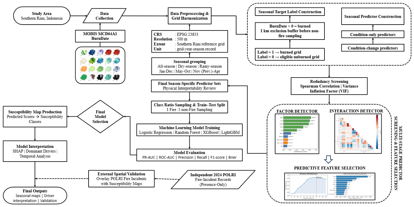
Figure 2.
Location, administrative extent, and land-cover context of the Southern Riau study area in Riau Province, Sumatra, Indonesia, comprising Kuantan Singingi, Indragiri Hulu, Indragiri Hilir, and Pelalawan regencies.
Figure 2.
Location, administrative extent, and land-cover context of the Southern Riau study area in Riau Province, Sumatra, Indonesia, comprising Kuantan Singingi, Indragiri Hulu, Indragiri Hilir, and Pelalawan regencies.
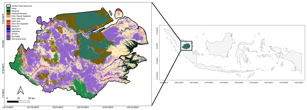
Figure 3.
Multi-metric comparison of the 24 candidate model configurations under the stratified 70:30 train–test split and 1:5 fire-to-non-fire sampling design. Stars indicate the final selected model for each modelling period. Colour intensity represents relative performance within each metric, with darker shading indicating better performance; Brier score was inversely scaled because lower values indicate better probabilistic performance.
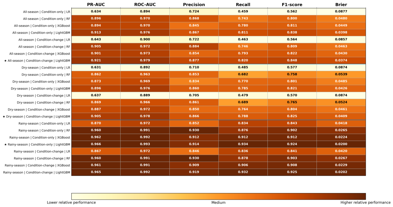
Figure 4.
Seasonal wildfire susceptibility maps of Southern Riau in 2024: (a) all-season, (b) dry-season, and (c) rainy-season. Susceptibility classes were defined separately for each modelling period using percentile thresholds of 30, 50, 80, and 95.
Figure 4.
Seasonal wildfire susceptibility maps of Southern Riau in 2024: (a) all-season, (b) dry-season, and (c) rainy-season. Susceptibility classes were defined separately for each modelling period using percentile thresholds of 30, 50, 80, and 95.
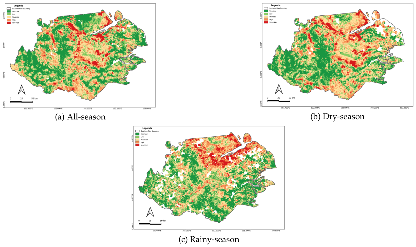
Figure 5.
SHAP contribution summaries of the final seasonal LightGBM wildfire-susceptibility models: (a) all-season, (b) dry-season, and (c) rainy-season. Predictor importance is ranked by mean absolute SHAP value, while the horizontal distribution and colour variation indicate the magnitude and direction of model-derived contributions across observations.
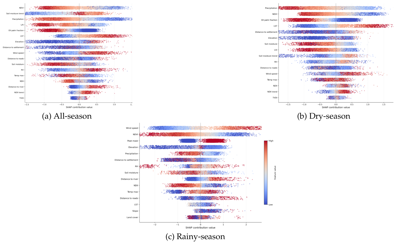
Figure 6.
Spatial distribution of SHAP-based dominant drivers across Southern Riau in 2024 for (a) all-season, (b) dry-season, and (c) rainy-season. Each mapped cell represents the predictor with the largest positive SHAP contribution under the corresponding final seasonal model.
Figure 6.
Spatial distribution of SHAP-based dominant drivers across Southern Riau in 2024 for (a) all-season, (b) dry-season, and (c) rainy-season. Each mapped cell represents the predictor with the largest positive SHAP contribution under the corresponding final seasonal model.
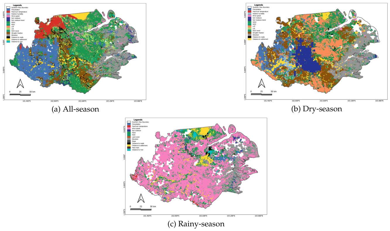
Figure 7.
Interannual variation in predicted wildfire-susceptibility class proportions and MODIS MCD64A1 burned area from 2010 to 2024 for the all-season, dry-season, and rainy-season modelling periods. The stacked areas represent the proportion of valid mapped area within each susceptibility class, while the black line represents detected burned area within the corresponding seasonal period.
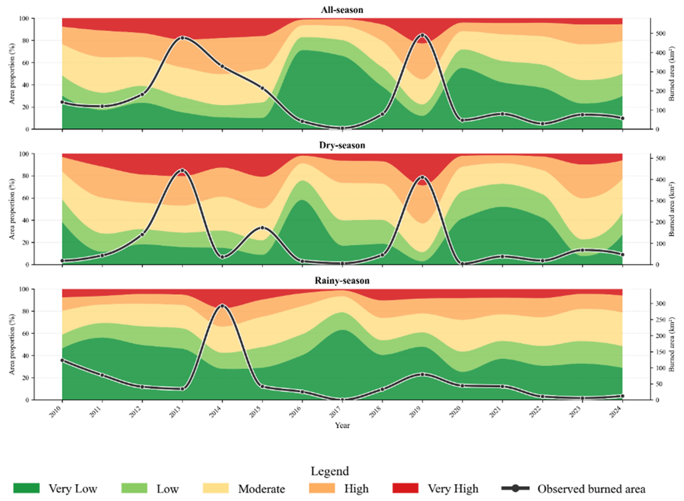
Figure 8.
Spatial correspondence between independent 2024 fire-incident records from the Indonesian National Police (POLRI) and predicted wildfire-susceptibility classes for (a) all-season, (b) dry-season, and (c) rainy-season validation subsets. POLRI records were used as presence-only independent spatial validation; therefore, the comparison evaluates whether documented fire incidents were concentrated within higher-ranked susceptibility classes rather than providing a complete external classification-accuracy assessment.
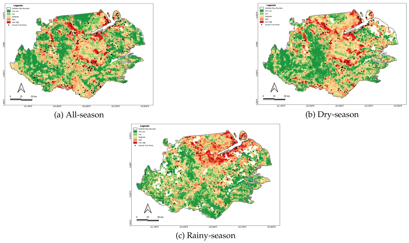

Table 1.
Main datasets used for seasonal wildfire susceptibility modelling in Southern Riau.
| Dataset | Source | Variable(s) | Period | Native resolution |
|---|---|---|---|---|
| MCD64A1 | NASA MODIS / GEE | BurnDate | 2010–2024 | 500 m |
| CHIRPS Pentad | UCSB-CHG / GEE | Precipitation | 2010–2024 | 5,566 m |
| TerraClimate | University of Idaho / GEE | Temperature, relative humidity, wind speed, and soil moisture | 2000–2024 | 4,638.3 m |
| MOD13Q1 | NASA MODIS / GEE | NDVI | 2000–2024 | 250 m |
| MOD09A1 | NASA MODIS / GEE | NDII | 2000–2024 | 500 m |
| MOD11A2 | NASA MODIS / GEE | Daytime LST | 2000–2024 | 1,000 m |
| TVDI | Derived from MOD13Q1 and MOD11A2 | TVDI | 2000–2024 | 1,000 m (LST-constrained) |
| MOD15A2H | NASA MODIS / GEE | LAI | 2000–2024 | 500 m |
| MCD12Q1 | NASA MODIS / GEE | Land-cover class | 2010–2024 | 500 m |
| SRTM + HydroSHEDS | NASA SRTM / HydroSHEDS / GEE | Elevation, slope, aspect, and TWI | Static | 30 m / 463.83 m |
| RBI vectors | BIG / Ina-Geoportal | Distances to roads, rivers, and settlements | Static | 1:50,000 vector |
| Peat polygon | BIG / Ina-Geoportal | Peat mask | Static | Vector polygon |
| MapBiomas Indonesia | Collection 4.1 | Oil-palm fraction | 2010–2024 | ∼30 m |
| POLRI incidents | Indonesian National Police | Coordinates, date, and incident information | 2024 | Point records |
Table 2.
Final sampled datasets and stratified 70:30 train–test composition.
| Period | Fire | Non-fire | Total | Train F/NF | Train total | Test F/NF | Test total |
|---|---|---|---|---|---|---|---|
| All-season | 6,514 | 32,570 | 39,084 | 4,560 / 22,798 | 27,358 | 1,954 / 9,772 | 11,726 |
| Dry-season | 3,428 | 17,140 | 20,568 | 2,400 / 11,997 | 14,397 | 1,028 / 5,143 | 6,171 |
| Rainy-season | 1,665 | 8,325 | 9,990 | 1,166 / 5,827 | 6,993 | 499 / 2,498 | 2,997 |
F = fire; NF = operational non-fire.
Table 3.
Fixed hyperparameters used in the machine-learning model comparison.
| Model | Role | Fixed hyperparameters |
|---|---|---|
| Logistic Regression | Regularized linear baseline | penalty = L2; C = 1.0; solver = saga; max_iter = 2000 |
| Random Forest | Bagging-based tree ensemble | n_estimators = 300; max_depth = 22; min_samples_leaf = 5; max_features = sqrt |
| XGBoost | Gradient-boosting tree ensemble | n_estimators = 500; learning_rate = 0.03; max_depth = 5; min_child_weight = 5; subsample = 0.8; colsample_bytree = 0.8 |
| LightGBM | Gradient-boosting tree ensemble | n_estimators = 500; learning_rate = 0.03; num_leaves = 31; max_depth = 8; min_child_samples = 30; subsample = 0.8; colsample_bytree = 0.8 |
Table 4.
Final predictor sets by modelling period and predictor configuration.
| Period | Configuration | No. | Final predictors |
|---|---|---|---|
| All-season | Condition-only | 16 | Precipitation, maximum temperature, relative humidity, wind speed, soil moisture, NDVI, NDII, LST, LAI, TVDI, oil-palm fraction, distance to river, distance to roads, distance to settlements, elevation, slope |
| All-season | Condition-change | 17 | Precipitation, maximum temperature, relative humidity, wind speed, soil moisture, NDVI, NDII, LST, LAI, TVDI, oil-palm fraction, distance to river, distance to roads, distance to settlements, elevation, NDII trend, soil-moisture trend |
| Dry-season | Condition-only | 15 | Precipitation, maximum temperature, relative humidity, wind speed, soil moisture, NDVI, NDII, LST, LAI, TVDI, oil-palm fraction, distance to river, distance to roads, distance to settlements, elevation |
| Dry-season | Condition-change | 16 | Precipitation, maximum temperature, relative humidity, wind speed, soil moisture, NDVI, NDII, LST, LAI, TVDI, oil-palm fraction, distance to roads, distance to settlements, elevation, NDII trend, soil-moisture trend |
| Rainy-season | Condition-only | 15 | Precipitation, maximum temperature, relative humidity, wind speed, soil moisture, NDVI, NDII, LST, land cover, distance to river, distance to roads, distance to settlements, peat mask, elevation, slope |
| Rainy-season | Condition-change | 17 | Precipitation, maximum temperature, relative humidity, wind speed, soil moisture, NDVI, NDII, LST, land cover, distance to river, distance to roads, distance to settlements, peat mask, elevation, slope, NDII trend, soil-moisture trend |
Condition-change predictor sets were screened separately and therefore were not necessarily supersets of their condition-only counterparts; retained historical trend indicators are shown explicitly.
Table 5.
Held-out comparative performance of the selected seasonal wildfire susceptibility models.
| Period | Final model | PR-AUC | ROC-AUC | Precision | Recall | F1-score | Brier score |
|---|---|---|---|---|---|---|---|
| All-season | LightGBM + Condition-change | 0.921 | 0.979 | 0.877 | 0.820 | 0.848 | 0.0374 |
| Dry-season | LightGBM + Condition-change | 0.905 | 0.978 | 0.866 | 0.788 | 0.825 | 0.0409 |
| Rainy-season | LightGBM + Condition-only | 0.966 | 0.993 | 0.914 | 0.934 | 0.924 | 0.0200 |
Table 6.
Leading global SHAP predictors and seasonal model-derived contribution structures.
| Period | Leading global SHAP predictors | Main contribution structure |
|---|---|---|
| All-season | NDVI; soil-moisture trend; precipitation; LAI; oil-palm fraction; LST | Vegetation condition, longer-term moisture change, rainfall deficit, land-use context, and surface heat |
| Dry-season | Precipitation; NDVI; oil-palm fraction; LST; distance to settlement; elevation; soil moisture | Rainfall deficit, vegetation condition, surface heating, soil drying, and land-use or accessibility context |
| Rainy-season | Wind speed; NDVI; peat mask; elevation; precipitation; distance to settlement | Wind-related conditions, vegetation condition, rainfall variability, and lowland or peat-related context |
Table 7.
Selected major and divergent years in the interannual susceptibility assessment.
| Period | Year | High + Very High (%) | Burned-area reference () | Main pattern |
|---|---|---|---|---|
| All-season | 2013 | 44.38 | 476.50 | Broad upper-susceptibility extent with strong burned-area signal |
| All-season | 2015 | 45.64 | 214.75 | Elevated upper-susceptibility extent |
| All-season | 2019 | 54.96 | 490.25 | Largest all-season upper-susceptibility extent and strongest burned-area signal |
| Dry-season | 2013 | 46.93 | 442.00 | Largest dry-season burned-area signal |
| Dry-season | 2015 | 49.43 | 173.25 | Elevated dry-season susceptibility |
| Dry-season | 2019 | 62.91 | 410.50 | Largest dry-season upper-susceptibility extent |
| Dry-season | 2023 | 40.28 | 68.00 | High susceptibility with limited detected burning |
| Rainy-season | 2014 | 34.05 | 292.75 | Largest rainy-season burned-area signal |
| Rainy-season | 2024 | 21.32 | 12.25 | Upper susceptibility with low detected burning |
High + Very High (%) was calculated relative to valid mapped area. MCD64A1 burned area was used only as an internal temporal reference and not as independent validation.
Table 8.
External-validation summary using independent 2024 POLRI fire-incident records.
| Period | Total | Matched | No match | Very Low | Low | Moderate | High | Very High | High + VH | High + VH (%) |
|---|---|---|---|---|---|---|---|---|---|---|
| All-season | 441 | 433 | 8 | 23 | 17 | 57 | 194 | 142 | 336 | 77.60 |
| Dry-season | 244 | 237 | 7 | 7 | 8 | 40 | 98 | 84 | 182 | 76.79 |
| Rainy-season | 197 | 196 | 1 | 16 | 9 | 17 | 96 | 58 | 154 | 78.57 |
High + VH (%) was calculated using matched records only. No match denotes incident records without an extractable valid susceptibility class. VH = Very High.
Disclaimer/Publisher’s Note: The statements, opinions and data contained in all publications are solely those of the individual author(s) and contributor(s) and not of MDPI and/or the editor(s). MDPI and/or the editor(s) disclaim responsibility for any injury to people or property resulting from any ideas, methods, instructions or products referred to in the content. |
© 2026 by the authors. Licensee MDPI, Basel, Switzerland. This article is an open access article distributed under the terms and conditions of the Creative Commons Attribution (CC BY) license (http://creativecommons.org/licenses/by/4.0/).
Copyright: This open access article is published under a Creative Commons CC BY 4.0 license, which permit the free download, distribution, and reuse, provided that the author and preprint are cited in any reuse.