Exact Solutions of the Free Dirac Equation via Separation of Variables on the Light-Front

1. Introduction

The Dirac equation plays a fundamental role in the relativistic description of spin-$1/2$ particles, combining the principles of quantum mechanics with relativistic invariance. Although it is usually formulated in Minkowski spacetime, different choices of the evolution surface can be employed in relativistic dynamics. In this context, [1] identified different forms of dynamics, including the front form, defined on a null hypersurface of spacetime.

The light-front coordinate formulation was subsequently developed as an alternative approach to relativistic systems. In their study of quantum electrodynamics in the infinite-momentum frame, [2] showed that this limit can be interpreted in terms of an appropriate change of variables, contributing to the development of the associated canonical formulation. Since then, light-front dynamics has been extensively studied both at the foundational level and in applications to field theory and relativistic systems, as discussed, for example, in the reviews [3,4,5,6,7,8].

In light-front coordinates, the longitudinal combinations $x^{+}$ and $x^{-}$ replace the usual temporal and longitudinal coordinates, while the transverse coordinates remain unchanged. This transformation modifies the differential structure of relativistic equations. In particular, the d’Alembert operator contains a mixed derivative in the longitudinal coordinates, a feature that plays an important role when the Klein–Gordon–Fock (KGF) equation is solved by separation of variables. [9] showed that this structure requires an additional procedure to decouple the longitudinal dependences, which can be implemented by introducing a nonzero auxiliary parameter $\lambda$ and its inverse. In this way, the solution can be systematically constructed by separation of variables and related to the plane-wave form expressed in light-front coordinates.

For fermionic fields, the formulation has an additional structure. The Dirac matrices associated with the longitudinal coordinates have particular algebraic properties, and ${\gamma }^{+}$ is nilpotent and therefore noninvertible. Consequently, the Dirac equation cannot be directly rearranged as an evolution equation in $x^{+}$ for all four spinor components. Decomposing the fermionic field by means of light-front projectors separates the spinor components and establishes relations between the dynamical and constrained components. This structure is widely discussed in the literature on light-front dynamics and quantization, including [3,5,6,7,8].

Different strategies can be used to determine solutions of the Dirac equation in these coordinates. For example, [10] treated the light-front Dirac equation through an algebraic procedure, starting from a plane-wave dependence and treating the resulting equation as a linear system for the spinor components. This approach directly yields the structure of the solutions and highlights particular features associated with light-front coordinates.

A complementary possibility is not to assume the complete form of the plane-wave spinor solution from the outset, but instead to determine its spacetime dependence first from the second-order equations satisfied by the individual components. Since applying the conjugate operator to the Dirac equation leads to a KGF equation for each spinor component, separation of variables can be employed at this stage. However, a solution of the KGF equation is not automatically a solution of the original Dirac equation, because the first-order equation imposes additional relations among the spinor components. We must therefore return to the Dirac equation after determining the spacetime dependence and reconstruct the spinor structure consistently with these constraints.

In this context, our aim is to apply the separation-of-variables strategy to the construction of solutions of the free Dirac equation in light-front coordinates. We first show that each spinor component satisfies the corresponding KGF equation. We then solve this equation by separation of variables, paying particular attention to the mixed-derivative term and to the longitudinal decoupling implemented through the auxiliary parameter $\lambda$. Once the common spacetime dependence of the components has been determined, we return to the first-order Dirac equation and use the projectors ${\mathsf{\Lambda }}_{\pm }$ to establish the relations between the projected components and explicitly reconstruct the spinor structure, obtaining two linearly independent solutions for the plane-wave branch considered.

Our approach thus explicitly distinguishes two levels in the construction of the solution: determination of the spacetime dependence from the second-order equations satisfied by the components, and determination of the spinor structure subject to the first-order Dirac equation. This organization highlights the role of separation of variables in the light-front formulation and the need to make the scalar solutions compatible with the constraints imposed by the spinor structure of the original equation. The purpose of the procedure is not to introduce a new plane-wave form or a new dispersion relation, but to establish systematically the mathematical path from separation of the components to the construction of the corresponding spinor solutions.

2. Dirac Equation and Separation of Variables in Minkowski Spacetime

We first consider the free Dirac equation in Minkowski spacetime,

$$\left(i{\gamma }^{\mu }{\partial }_{\mu }-m\right)\psi \left(x\right)=0,$$

(1)

where the ${\gamma }^{\mu }$ matrices satisfy the anticommutation relation

$$\left\{{\gamma }^{\mu },{\gamma }^{\nu }\right\}=2{\eta }^{\mu \nu }{\mathbb{I}}_4.$$

(2)

We obtain the relation between the Dirac equation and the Klein–Gordon–Fock (KGF) equation by applying the operator $(i{\gamma }^{\nu }{\partial }_{\nu }+m)$ to Equation (1). Thus,

$$\left(i{\gamma }^{\nu }{\partial }_{\nu }+m\right)\left(i{\gamma }^{\mu }{\partial }_{\mu }-m\right)\psi \left(x\right)=0.$$

(3)

Since the ${\gamma }^{\mu }$ matrices are constant and the partial derivatives commute, the cross terms cancel, yielding

$$-{\gamma }^{\nu }{\gamma }^{\mu }{\partial }_{\nu }{\partial }_{\mu }\psi \left(x\right)-m^2\psi \left(x\right)=0.$$

(4)

Because ${\partial }_{\nu }{\partial }_{\mu }$ is symmetric in the indices $\mu$ and $\nu$, only the symmetric part of the product of Dirac matrices contributes. Using

$${\displaystyle \frac{1}{2}}\left({\gamma }^{\nu }{\gamma }^{\mu }+{\gamma }^{\mu }{\gamma }^{\nu }\right)={\eta }^{\mu \nu }{\mathbb{I}}_4,$$

(5)

we obtain

$$\left({\eta }^{\mu \nu }{\partial }_{\mu }{\partial }_{\nu }+m^2\right)\psi \left(x\right)=0,$$

(6)

or, equivalently,

$$\left(\square +m^2\right)\psi \left(x\right)=0,$$

(7)

where $\square ={\partial }_t^2-{\nabla }^2$ denotes the d’Alembert operator.

Therefore, each of the four spinor components,

$$\psi \left(x\right)=\left(\begin{array}{c}{\psi }_1\left(x\right)\\ {\psi }_2\left(x\right)\\ {\psi }_3\left(x\right)\\ {\psi }_4\left(x\right)\end{array}\right),$$

(8)

individually satisfies the KGF equation

$$\left(\square +m^2\right){\psi }_j\left(x\right)=0,j=1,2,3,4.$$

(9)

This result allows us to use separation of variables to determine the spacetime dependence of the spinor components in Equation (8). For a generic component, we write

$${\psi }_j(t,x,y,z)=T_j\left(t\right)X_j\left(x\right)Y_j\left(y\right)Z_j\left(z\right),j=1,2,3,4.$$

(10)

Substituting Equation (10) into Equation (9) and dividing by the product $T_j{X}_j{Y}_j{Z}_j$, we obtain

$${\displaystyle \frac{T_j^{\prime \prime }}{T_j}}-{\displaystyle \frac{X_j^{\prime \prime }}{X_j}}-{\displaystyle \frac{Y_j^{\prime \prime }}{Y_j}}-{\displaystyle \frac{Z_j^{\prime \prime }}{Z_j}}+m^2=0.$$

(11)

Separating the spatial and temporal dependences leads to

$$\left\{\begin{array}{ccc}\hfill X_j^{\prime \prime }+p_{x_j}^2{X}_j& =& 0\hfill \\ \\ \hfill Y_j^{\prime \prime }+p_{y_j}^2{Y}_j& =& 0\hfill \\ \\ \hfill Z_j^{\prime \prime }+p_{z_j}^2{Z}_j& =& 0\hfill \end{array}\right.,$$

(12)

and

$$T_j^{″}+\left(p_{x_j}^2+p_{y_j}^2+p_{z_j}^2+m^2\right)T_j=0.$$

(13)

In Equation (13), since ${\mathbf{p}}_j^2=p_{x_j}^2+p_{y_j}^2+p_{z_j}^2$ and $E_j^2={\mathbf{p}}_j^2+m^2$, we have

$$T_j^{″}+E_j^2{T}_j=0.$$

(14)

Solving Equations (12) and (14), we obtain

$$\begin{array}{ccc}\hfill X_j\left(x\right)& =& A_{x_j}{e}^{i{p}_{x_j}x}+B_{x_j}{e}^{-i{p}_{x_j}x}\hfill \\ \\ \hfill Y_j\left(y\right)& =& A_{y_j}{e}^{i{p}_{y_j}y}+B_{y_j}{e}^{-i{p}_{y_j}y}\hfill \\ \\ \hfill Z_j\left(z\right)& =& A_{z_j}{e}^{i{p}_{z_j}z}+B_{z_j}{e}^{-i{p}_{z_j}z}\hfill \\ \\ \hfill T_j\left(t\right)& =& A_{t_j}{e}^{-i{E}_{j}t}+B_{t_j}{e}^{i{E}_{j}t}\hfill \end{array},j=1,2,3,4.$$

(15)

For the branch considered here, we may set $B_{x_j}=B_{y_j}=B_{z_j}=B_{t_j}=0$, so that

$$\begin{array}{ccc}\hfill X_j\left(x\right)& =& A_{x_j}{e}^{i{p}_{x_j}x}\hfill \\ \\ \hfill Y_j\left(y\right)& =& A_{y_j}{e}^{i{p}_{y_j}y}\hfill \\ \\ \hfill Z_j\left(z\right)& =& A_{z_j}{e}^{i{p}_{z_j}z}\hfill \\ \\ \hfill T_j\left(t\right)& =& A_{t_j}{e}^{-i{E}_{j}t}\hfill \end{array},j=1,2,3,4.$$

(16)

Substituting Equation (16) into Equation (10), we find

$$\begin{array}{ccc}\hfill {\psi }_j(t,x,y,z)& =& A_j{e}^{-i\left(E_{j}t-p_{x_j}x-p_{y_j}y-p_{z_j}z\right)}\hfill \\ & =& A_j{e}^{-i\left(E_{j}t-{\mathbf{p}}_j\mathbf{x}\right)},j=1,2,3,4,\hfill \end{array}$$

(17)

where $A_j=A_{x_j}{A}_{y_j}{A}_{z_j}{A}_{t_j}$.

The KGF equation (9) therefore determines the spacetime dependence of each component. However, the constants $A_j$ cannot be chosen arbitrarily when these components belong to the same solution of the Dirac equation. In particular, for a given spinor mode, different values of $E_j$ and $p_j$ should not be assigned arbitrarily to each component. The Dirac equation requires the components of the same mode to share a common spacetime factor, namely,

$$\psi (t,\mathbf{x})=U\left(p\right)e^{-i\left(Et-p\mathbf{x}\right)},$$

(18)

where $p=(p_x,p_y,p_z)$ and $\mathbf{x}=(x,y,z)$, with

$$U\left(p\right)=\left(\begin{array}{c}{u}_1\\ u_2\\ u_3\\ u_4\end{array}\right).$$

(19)

At this stage, we return to the Dirac equation (1). Substituting Equation (18) into Equation (1) and using

$${\partial }_{\mu }{e}^{-ipx}=-i{p}_{\mu }{e}^{-ipx},$$

(20)

we obtain

$$\left({\gamma }^{\mu }{p}_{\mu }-m\right)U\left(p\right)=0.$$

(21)

Separation of variables determines the common spacetime factor, whereas the algebraic equation (21) establishes the relations among the amplitudes that form the spinor (19).

To make these relations explicit, we adopt the Dirac representation,

$${\gamma }^0=\left(\begin{array}{cc}{\mathbb{I}}_2& 0\\ 0& -{\mathbb{I}}_2\end{array}\right),{\gamma }^i=\left(\begin{array}{cc}0& {\sigma }^i\\ -{\sigma }^i& 0\end{array}\right),$$

(22)

where ${\mathbb{I}}_2$ is the $2\times 2$ identity matrix and ${\sigma }^i$, with $i=1,2,3$, are the Pauli matrices,

$${\sigma }^1=\left(\begin{array}{cc}0& 1\\ 1& 0\end{array}\right);{\sigma }^2=\left(\begin{array}{cc}0& -i\\ i& 0\end{array}\right);{\sigma }^3=\left(\begin{array}{cc}1& 0\\ 0& -1\end{array}\right).$$

(23)

We write the spinor (19) as

$$U\left(p\right)=\left(\begin{array}{c}\varphi \\ \chi \end{array}\right),$$

(24)

where

$$\varphi =\left(\begin{array}{c}{u}_1\\ u_2\end{array}\right),\chi =\left(\begin{array}{c}{u}_3\\ u_4\end{array}\right).$$

(25)

The algebraic equation (21) then becomes

$$\left(\begin{array}{cc}\left(E-m\right){\mathbb{I}}_2& -{\sigma }^i·p\\ {\sigma }^i·p& -\left(E+m\right){\mathbb{I}}_2\end{array}\right)\left(\begin{array}{c}\varphi \\ \chi \end{array}\right)=\left(\begin{array}{c}0\\ 0\end{array}\right).$$

(26)

Equation (26) yields the system

$$\begin{array}{ccc}\hfill \left(E-m\right)\varphi -\left({\sigma }^i·p\right)\chi & =& 0,\hfill \end{array}$$

(27)

$$\begin{array}{ccc}\hfill \left({\sigma }^i·p\right)\varphi -\left(E+m\right)\chi & =& 0.\hfill \end{array}$$

(28)

For $E>0$, Equation (28) gives

$$\chi ={\displaystyle \frac{{\sigma }^i·p}{E+m}}\varphi .$$

(29)

Substituting Equation (29) into Equation (27), we obtain

$$\left[\left(E-m\right)-{\displaystyle \frac{{\left({\sigma }^i·p\right)}^2}{E+m}}\right]\varphi =0.$$

(30)

Since

$${\left({\sigma }^i·p\right)}^2=p^2{\mathbb{I}}_2,$$

(31)

it follows that

$$E^2-p^2-m^2=0,$$

(32)

which recovers the dispersion relation obtained from the KGF equation (7), in agreement with [9]. The compatibility between the two equations is therefore explicitly verified.

The spinor (24) can then be written as

$$U\left(p\right)=\left(\begin{array}{c}\varphi \\ {\displaystyle \frac{{\sigma }^i·p}{E+m}}\varphi \end{array}\right).$$

(33)

Since $\varphi$ has two independent components, we choose the basis

$${\varphi }_1=\left(\begin{array}{c}1\\ 0\end{array}\right),{\varphi }_2=\left(\begin{array}{c}0\\ 1\end{array}\right).$$

(34)

Using

$${\sigma }^i·p=\left(\begin{array}{cc}{p}_z& p_x-i{p}_y\\ p_x+i{p}_y& -p_z\end{array}\right),$$

(35)

we obtain two linearly independent spinor solutions,

$$U_1\left(p\right)=\left(\begin{array}{c}1\\ 0\\ {\displaystyle \frac{p_z}{E+m}}\\ {\displaystyle \frac{p_x+i{p}_y}{E+m}}\end{array}\right)$$

(36)

and

$$U_2\left(p\right)=\left(\begin{array}{c}0\\ 1\\ {\displaystyle \frac{p_x-i{p}_y}{E+m}}\\ -{\displaystyle \frac{p_z}{E+m}}\end{array}\right).$$

(37)

Thus, for $E>0$, the solutions of the Dirac equation (1) can be expressed as

$$\psi \left(x\right)=N_s{U}_s\left(p\right)e^{-i\left(Et-px\right)},s=1,2,$$

(38)

where $N_s$ denotes a normalization factor whose explicit choice is not required for the construction considered in this work.

The preceding derivation highlights the distinction between the two stages that we also use in the light-front formulation. The KGF equation (7) associated with the components determines, through separation of variables, the spacetime dependence and the corresponding dispersion relation. Returning to the Dirac equation (1) then imposes relations among the component amplitudes and determines the spinor structure. In Minkowski spacetime, separation proceeds directly because the second-order derivatives appear separately in the temporal and spatial coordinates. In the light-front formulation, however, the mixed term $2{\partial }_{+}{\partial }_{-}$ changes this structure and requires an additional procedure to separate the dependences associated with the longitudinal coordinates $x^{+}$ and $x^{-}$. This difference provides the starting point for the developments in the following sections.

3. Free Dirac Equation in Light-Front Coordinates

For the longitudinal components, we define the light-front coordinate system through the transformations

$$x^{+}={\displaystyle \frac{x^0+x^3}{\sqrt{2}}},x^{-}={\displaystyle \frac{x^0-x^3}{\sqrt{2}}},$$

(39)

while the transverse coordinates retain the form

$$x^{\perp }=(x^1,x^2).$$

(40)

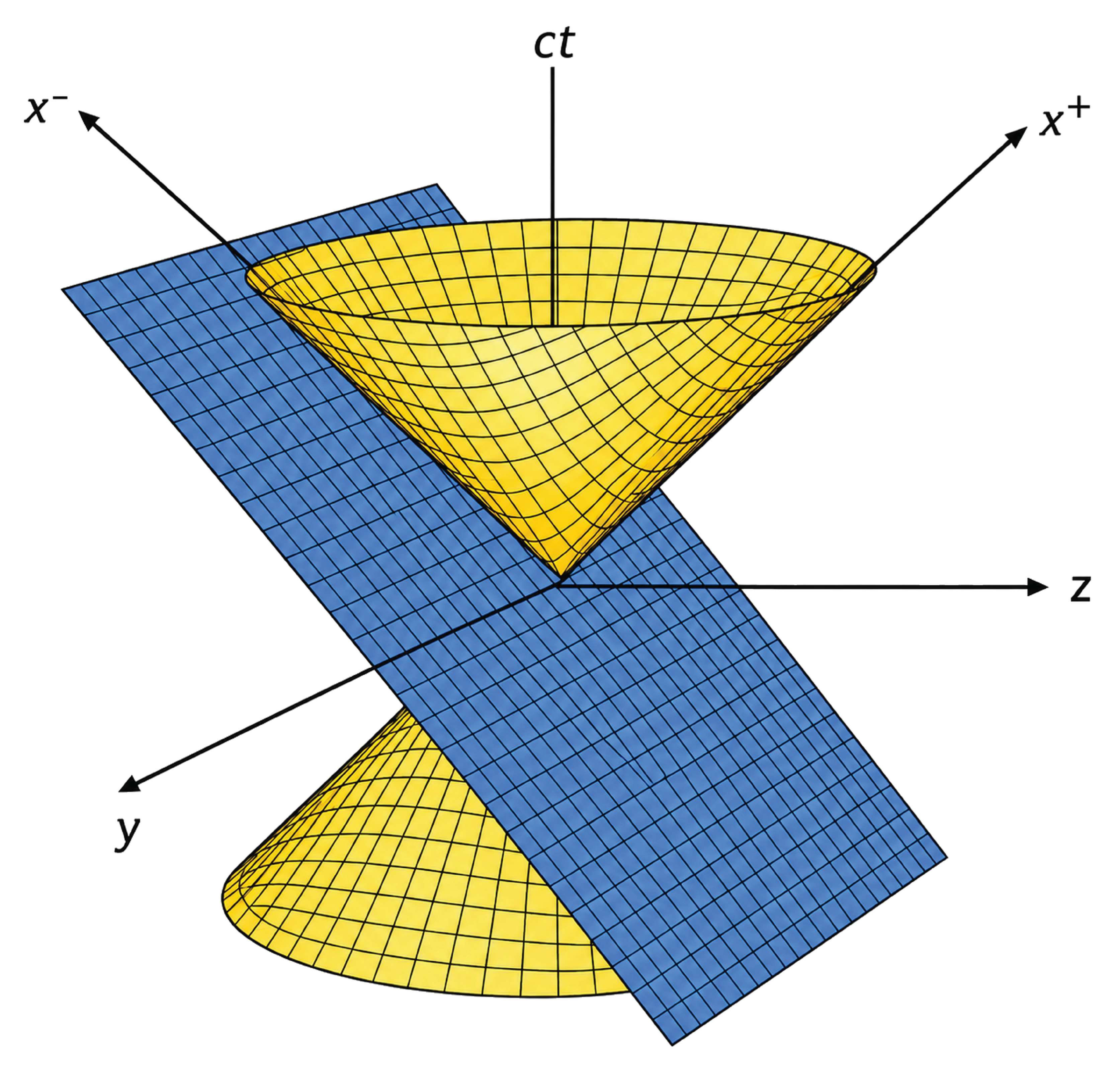
Figure 1 shows a geometric representation of the relativistic light cone (in yellow) and the plane associated with the light-front coordinate system [1]. The $x^{+}$ and $x^{-}$ axes indicate the characteristic directions of the formulation, while the highlighted plane (in blue) represents a light-front hypersurface.

The inverse transformations are

$$x^0={\displaystyle \frac{x^{+}+x^{-}}{\sqrt{2}}},x^3={\displaystyle \frac{x^{+}-x^{-}}{\sqrt{2}}}.$$

(41)

Similarly, for the four-momentum $p^{\mu }=(p^0,p^1,p^2,p^3)$, we define

$$p^{+}={\displaystyle \frac{p^0+p^3}{\sqrt{2}}},p^{-}={\displaystyle \frac{p^0-p^3}{\sqrt{2}}},$$

(42)

and

$$p^{\perp }=(p^1,p^2).$$

(43)

The corresponding inverse relations are

$$p^0={\displaystyle \frac{p^{+}+p^{-}}{\sqrt{2}}},p^3={\displaystyle \frac{p^{+}-p^{-}}{\sqrt{2}}}.$$

(44)

With these definitions, we can rewrite the Minkowski scalar product as

$$p_{\mu }{x}^{\mu }=p^0{x}^0-p^1{x}^1-p^2{x}^2-p^3{x}^3,$$

(45)

which gives

$$p_{\mu }{x}^{\mu }=p^{-}{x}^{+}+p^{+}{x}^{-}-p^{\perp }{x}^{\perp }.$$

(46)

Equation (46) will be particularly important when we identify the spacetime dependence obtained later through separation of variables.

We obtain the derivatives with respect to the new coordinates by applying the chain rule. From the inverse transformations, we find

$${\partial }_{+}\equiv {\displaystyle \frac{\partial }{\partial x^{+}}}={\displaystyle \frac{1}{\sqrt{2}}}({\partial }_0+{\partial }_3),$$

(47)

and

$${\partial }_{-}\equiv {\displaystyle \frac{\partial }{\partial x^{-}}}={\displaystyle \frac{1}{\sqrt{2}}}({\partial }_0-{\partial }_3).$$

(48)

Consequently,

$${\partial }_0={\displaystyle \frac{{\partial }_{+}+{\partial }_{-}}{\sqrt{2}}},{\partial }_3={\displaystyle \frac{{\partial }_{+}-{\partial }_{-}}{\sqrt{2}}}.$$

(49)

For the transverse coordinates, we use

$${\partial }_{\perp }=({\partial }_1,{\partial }_2),{\partial }_{\perp }^2={\partial }_1^2+{\partial }_2^2.$$

(50)

The d’Alembert operator,

$$\square ={\partial }_0^2-{\partial }_1^2-{\partial }_2^2-{\partial }_3^2,$$

(51)

therefore takes the form

$$\begin{array}{cc}\hfill \square & ={\displaystyle \frac{1}{2}}{({\partial }_{+}+{\partial }_{-})}^2-{\displaystyle \frac{1}{2}}{({\partial }_{+}-{\partial }_{-})}^2-{\partial }_{\perp }^2\hfill \\ \hfill & =2{\partial }_{+}{\partial }_{-}-{\partial }_{\perp }^2.\hfill \end{array}$$

Thus,

$$\square =2{\partial }_{+}{\partial }_{-}-{\partial }_{\perp }^2.$$

(52)

Equation (52) highlights an essential feature of the light-front formulation: unlike the usual expression $\square ={\partial }_t^2-{\nabla }^2$, the longitudinal coordinates $x^{+}$ and $x^{-}$ are coupled through the mixed derivative $2{\partial }_{+}{\partial }_{-}$. This structure directly affects the separation-of-variables procedure developed in the next section.

To write the Dirac equation (1) in light-front coordinates, we also define

$${\gamma }^{+}={\displaystyle \frac{{\gamma }^0+{\gamma }^3}{\sqrt{2}}},{\gamma }^{-}={\displaystyle \frac{{\gamma }^0-{\gamma }^3}{\sqrt{2}}},$$

(53)

where

$${\gamma }^{+}={\displaystyle \frac{1}{\sqrt{2}}}\left(\begin{array}{cccc}1& 0& 1& 0\\ 0& 1& 0& -1\\ -1& 0& -1& 0\\ 0& 1& 0& -1\end{array}\right),{\gamma }^{-}={\displaystyle \frac{1}{\sqrt{2}}}\left(\begin{array}{cccc}1& 0& -1& 0\\ 0& 1& 0& 1\\ 1& 0& -1& 0\\ 0& -1& 0& -1\end{array}\right).$$

Using the Clifford algebra together with

$${\left({\gamma }^0\right)}^2={\mathbb{I}}_4,{\left({\gamma }^3\right)}^2=-{\mathbb{I}}_4,\left\{{\gamma }^0,{\gamma }^3\right\}=0,$$

(54)

we obtain

$${\left({\gamma }^{+}\right)}^2={\displaystyle \frac{1}{2}}\left[{\left({\gamma }^0\right)}^2+{\left({\gamma }^3\right)}^2+\left\{{\gamma }^0,{\gamma }^3\right\}\right]=0,$$

(55)

and, analogously,

$${\left({\gamma }^{-}\right)}^2=0.$$

(56)

Therefore,

$${\left({\gamma }^{+}\right)}^2={\left({\gamma }^{-}\right)}^2=0.$$

(57)

Moreover,

$$\left\{{\gamma }^{+},{\gamma }^{-}\right\}={\displaystyle \frac{1}{2}}\left\{{\gamma }^0+{\gamma }^3,{\gamma }^0-{\gamma }^3\right\}=2{\mathbb{I}}_4,$$

(58)

so that

$$\left\{{\gamma }^{+},{\gamma }^{-}\right\}=2{\mathbb{I}}_4.$$

(59)

The properties in Eqs. (57) and (59) will be important later when we decompose the Dirac equation into projected components.

Starting again from the covariant Dirac equation (1), we transform the longitudinal part of the Dirac operator using

$${\gamma }^0{\partial }_0+{\gamma }^3{\partial }_3={\gamma }^{+}{\partial }_{+}+{\gamma }^{-}{\partial }_{-}.$$

(60)

Substituting Eq. (60) into the expanded form of Eq. (1), we obtain the Dirac equation in light-front coordinates:

$$\left(i{\gamma }^{+}{\partial }_{+}+i{\gamma }^{-}{\partial }_{-}+i{\gamma }^{\perp }·{\partial }_{\perp }-m\right){\psi }_{\mathrm{LF}}=0,$$

(61)

where

$${\gamma }^{\perp }=({\gamma }^1,{\gamma }^2),{\gamma }^{\perp }·{\partial }_{\perp }={\gamma }^1{\partial }_1+{\gamma }^2{\partial }_2.$$

(62)

As in the Minkowski case, we obtain the associated second-order equation by applying to Eq. (61) the operator with the opposite sign of the mass term,

$$i{\gamma }^{+}{\partial }_{+}+i{\gamma }^{-}{\partial }_{-}+i{\gamma }^{\perp }·{\partial }_{\perp }+m,$$

(63)

and using the anticommutation relations of the Dirac matrices in Eq. (2). This gives

$$\left(2{\partial }_{+}{\partial }_{-}-{\partial }_{\perp }^2+m^2\right){\psi }_{\mathrm{LF}}=0.$$

(64)

Therefore, writing

$${\psi }_{\mathrm{LF}}=\left(\begin{array}{c}{\psi }_{{\mathrm{LF}}_1}\\ {\psi }_{{\mathrm{LF}}_2}\\ {\psi }_{{\mathrm{LF}}_3}\\ {\psi }_{{\mathrm{LF}}_4}\end{array}\right),$$

(65)

we find that each component individually satisfies

$$\left(2{\partial }_{+}{\partial }_{-}-{\partial }_{\perp }^2+m^2\right){\psi }_{{\mathrm{LF}}_j}=0,j=1,2,3,4.$$

(66)

Equation (66), the Klein–Gordon–Fock equation for each light-front spinor component, provides the starting point for applying the same strategy used in the previous section. However, as discussed in [9], separating the longitudinal variables requires an additional decoupling step. At this stage, we introduce the nonzero auxiliary parameter $\lambda$, which allows us to determine the $x^{+}$ and $x^{-}$ dependences separately and reconstruct the plane-wave phase in light-front coordinates.

4. Separation of Variables and the Light-Front Plane-Wave Phase

As established in the previous section, each component of the Dirac spinor (65) satisfies the Klein–Gordon–Fock equation (66) in light-front coordinates. Since the differential equation has the same form for all components, we first consider a generic function ${\psi }_{\mathrm{LF}}(x^{+},x^{-},x^{\perp })$ satisfying

$$\left(2{\partial }_{+}{\partial }_{-}-{\partial }_{\perp }^2+m^2\right){\psi }_{\mathrm{LF}}(x^{+},x^{-},x^{\perp })=0.$$

(67)

Following the separation-of-variables strategy, we assume a product solution of the form

$${\psi }_{\mathrm{LF}}(x^{+},x^{-},x^{\perp })=B\left(x^{+}\right)C\left(x^{-}\right)\eta \left(x^{\perp }\right).$$

(68)

Acting with the mixed derivative on (68), we first obtain

$${\partial }_{-}{\psi }_{\mathrm{LF}}=B\left(x^{+}\right)C^{\prime }\left(x^{-}\right)\eta \left(x^{\perp }\right)$$

(69)

and, consequently,

$${\partial }_{+}{\partial }_{-}{\psi }_{\mathrm{LF}}=B^{\prime }\left(x^{+}\right)C^{\prime }\left(x^{-}\right)\eta \left(x^{\perp }\right).$$

(70)

For the transverse part,

$${\partial }_{\perp }^2{\psi }_{\mathrm{LF}}=B\left(x^{+}\right)C\left(x^{-}\right){\partial }_{\perp }^2\eta \left(x^{\perp }\right).$$

(71)

Substituting Eqs. (70) and (71) into the KGF equation (67), we obtain

$$2B^{\prime }{C}^{\prime }\eta -BC{\partial }_{\perp }^2\eta +m^{2}BC\eta =0.$$

(72)

Dividing Eq. (72) by $BC\eta$, assuming that B, C, and $\eta$ are nonzero in the domain under consideration, gives

$$2{\displaystyle \frac{B^{\prime }}{B}}{\displaystyle \frac{C^{\prime }}{C}}-{\displaystyle \frac{{\partial }_{\perp }^2\eta }{\eta }}+m^2=0.$$

(73)

At this point, the main difference from the procedure carried out in Minkowski spacetime becomes apparent. The dependences associated with $x^{+}$ and $x^{-}$ do not appear as a sum of independent terms, but through the product ${\displaystyle \frac{B^{\prime }}{B}}{\displaystyle \frac{C^{\prime }}{C}}$, as a direct consequence of the mixed derivative $2{\partial }_{+}{\partial }_{-}$. Therefore, separating the two longitudinal variables requires an additional decoupling step.

We first separate the transverse dependence by introducing ${\left(p^{\perp }\right)}^2$ as a separation constant,

$${\partial }_{\perp }^2\eta +{\left(p^{\perp }\right)}^2\eta =0,$$

(74)

where ${\left(p^{\perp }\right)}^2={\left(p^1\right)}^2+{\left(p^2\right)}^2$. To construct an elementary plane-wave mode, we choose

$$\eta \left(x^{\perp }\right)=e^{i{p}^{\perp }{x}^{\perp }}.$$

(75)

It follows from Eq. (74) that

$${\displaystyle \frac{{\partial }_{\perp }^2\eta }{\eta }}=-{\left(p^{\perp }\right)}^2.$$

(76)

Substituting Eq. (76) into Eq. (73), the longitudinal equation becomes

$$2{\displaystyle \frac{B^{\prime }}{B}}{\displaystyle \frac{C^{\prime }}{C}}+{\left(p^{\perp }\right)}^2+m^2=0,$$

(77)

or

$${\displaystyle \frac{B^{\prime }}{B}}{\displaystyle \frac{C^{\prime }}{C}}=-{\displaystyle \frac{{\left(p^{\perp }\right)}^2+m^2}{2}}.$$

(78)

The dispersion relation for a free particle can be written in light-front coordinates as

$$2p^{+}{p}^{-}={\left(p^{\perp }\right)}^2+m^2.$$

(79)

Therefore, using Eq. (79), we rewrite Eq. (78) as

$${\displaystyle \frac{B^{\prime }}{B}}{\displaystyle \frac{C^{\prime }}{C}}=-p^{+}{p}^{-}.$$

(80)

Equation (80) contains the product of a function that depends only on $x^{+}$ and another that depends only on $x^{-}$. To make the decoupling explicit, for nonzero momentum components appearing in the denominators we define

$$f\left(x^{+}\right)={\displaystyle \frac{i}{p^{-}}}{\displaystyle \frac{B^{\prime }}{B}},g\left(x^{-}\right)={\displaystyle \frac{i}{p^{+}}}{\displaystyle \frac{C^{\prime }}{C}}.$$

(81)

It then follows that

$$f\left(x^{+}\right)g\left(x^{-}\right)=1.$$

(82)

Because f depends only on $x^{+}$ and g only on $x^{-}$, whereas their product must remain constant for independent values of these coordinates, each function must itself be constant. Following [9], we therefore introduce a nonzero auxiliary parameter $\lambda$ such that

$$f\left(x^{+}\right)=\lambda ,g\left(x^{-}\right)={\lambda }^{-1},\lambda \ne 0.$$

(83)

Thus,

$${\displaystyle \frac{B^{\prime }}{B}}=-i\lambda p^{-},{\displaystyle \frac{C^{\prime }}{C}}=-i{\lambda }^{-1}{p}^{+}.$$

(84)

Indeed,

$$\left(-i\lambda p^{-}\right)\left(-i{\lambda }^{-1}{p}^{+}\right)=-p^{-}{p}^{+},$$

(85)

so the original product is preserved. The parameter $\lambda$ therefore arises from decoupling the two longitudinal dependences; it does not represent a new coordinate or a dynamical variable.

Integrating the differential equations in (84), we obtain

$$B\left(x^{+}\right)=B_0{e}^{-i\lambda p^{-}{x}^{+}},C\left(x^{-}\right)=C_0{e}^{-i{\lambda }^{-1}{p}^{+}{x}^{-}}.$$

(86)

Hence, before selecting a particular value of $\lambda$, the separated mode (68) takes the form

$${\psi }_{\mathrm{LF}}(x^{+},x^{-},x^{\perp })=A{e}^{-i\lambda p^{-}{x}^{+}}{e}^{-i{\lambda }^{-1}{p}^{+}{x}^{-}}{e}^{i{p}^{\perp }{x}^{\perp }},$$

(87)

where $A=B_0{C}_0$ absorbs the multiplicative constants.

In the parametrization adopted in this work, we choose $\lambda =1$ so that the longitudinal constants are identified directly with $p^{-}$ and $p^{+}$. We then obtain

$${\psi }_{\mathrm{LF}}(x^{+},x^{-},x^{\perp })=A{e}^{-i\left(p^{-}{x}^{+}+p^{+}{x}^{-}-p^{\perp }{x}^{\perp }\right)}.$$

(88)

In Eq. (88), the argument of the exponential coincides precisely with the light-front scalar product obtained in Eq. (46).

Therefore, for each component of the spinor (65), we have

$${\psi }_{{\mathrm{LF}}_j}(x^{+},x^{-},x^{\perp })=A_j{e}^{-i\left(p^{-}{x}^{+}+p^{+}{x}^{-}-p^{\perp }{x}^{\perp }\right)},j=1,2,3,4.$$

(89)

We can therefore collect the components as

$${\psi }_{\mathrm{LF}}(x^{+},x^{-},x^{\perp })=U_{\mathrm{LF}}\left(p\right)e^{-i\left(p^{-}{x}^{+}+p^{+}{x}^{-}-p^{\perp }{x}^{\perp }\right)},$$

(90)

where

$$U_{\mathrm{LF}}\left(p\right)=\left(\begin{array}{c}{A}_1\\ A_2\\ A_3\\ A_4\end{array}\right).$$

(91)

At this stage, however, $U_{\mathrm{LF}}\left(p\right)$ is still undetermined. Applying the KGF equation (66) to the individual components determines their common spacetime dependence, but it does not establish the relations among the amplitudes $A_j$. As in the Minkowski case, a solution of the KGF equation for each component is not automatically a solution of the Dirac equation. We must return to the original first-order equation to determine which combinations of amplitudes are admissible.

In the light-front formulation, this return introduces an additional structure: the algebraic properties of the matrices ${\gamma }^{\pm }$ allow us to decompose the spinor using the projectors ${\mathsf{\Lambda }}_{\pm }$ and thereby establish relations between the projected components. These relations will allow us to reconstruct $U_{\mathrm{LF}}\left(p\right)$ and explicitly obtain the two linearly independent spinor solutions associated with the plane-wave branch considered here.

5. Reconstruction of the Light-Front Spinor

The separation of variables carried out in the previous section provided, for the branch considered here, the spacetime dependence

$$\psi \mathrm{LF}(x^{+},x^{-},x^{\perp })=U_{\mathrm{LF}}\left(p\right)e^{-i\left(p^{-}{x}^{+}+p^{+}{x}^{-}-p^{\perp }{x}^{\perp }\right)}.$$

(92)

However, the KGF equation (66) satisfied by the components does not, by itself, determine the relations among the amplitudes that constitute $U_{\mathrm{LF}}\left(p\right)$. To establish these relations, we return to the first-order Dirac equation (61),

$$\left(i{\gamma }^{+}{\partial }_{+}+i{\gamma }^{-}{\partial }_{-}+i{\gamma }^{\perp }·{\partial }_{\perp }-m\right){\psi }_{\mathrm{LF}}=0,$$

(93)

For the exponential dependence obtained in (92),

$${\partial }_{+}{\psi }_{\mathrm{LF}}=-i{p}^{-}{\psi }_{\mathrm{LF}},{\partial }_{-}{\psi }_{\mathrm{LF}}=-i{p}^{+}{\psi }_{\mathrm{LF}},{\partial }_{\perp }{\psi }_{\mathrm{LF}}=i{p}^{\perp }{\psi }_{\mathrm{LF}}.$$

(94)

Substituting the relations (94) into the Dirac equation (93) and canceling the common exponential factor, we obtain

$$\left({\gamma }^{+}{p}^{-}+{\gamma }^{-}{p}^{+}-{\gamma }^{\perp }·p^{\perp }-m\right)U_{\mathrm{LF}}\left(p\right)=0.$$

(95)

Equation (95) is the algebraic form of the Dirac equation (93) in light-front coordinates. It also provides the point of contact with approaches in which the spinor solution is constructed directly from the algebraic system resulting from an initial plane-wave ansatz, as in [10]. In our procedure, however, we do not assume this form at the outset: we have previously obtained the plane-wave dependence by applying separation of variables to the KGF equations satisfied by the components.

Reconstructing the spinor structure requires us to consider a particular property of the Dirac equation in light-front coordinates (93). Since $x^{+}$ plays the role of the light-front evolution coordinate, one might attempt to isolate ${\partial }_{+}{\psi }_{\mathrm{LF}}$ in the equation

$$i{\gamma }^{+}{\partial }_{+}{\psi }_{\mathrm{LF}}=\left(-i{\gamma }^{-}{\partial }_{-}-i{\gamma }^{\perp }·{\partial }_{\perp }+m\right){\psi }_{\mathrm{LF}}.$$

(96)

However, as shown previously in Equation (57),

$${\left({\gamma }^{+}\right)}^2=0,$$

(97)

that is, ${\gamma }^{+}$ is nilpotent and therefore singular. In particular,

$$det\left({\gamma }^{+}\right)=0,$$

(98)

so ${\left({\gamma }^{+}\right)}^{-1}$ does not exist. Therefore, we cannot obtain an evolution equation for all four spinor components simply by multiplying the preceding expression by the inverse of ${\gamma }^{+}$. This structure motivates the decomposition of spinor space into complementary subspaces through the projectors characteristic of the light-front fermionic formulation [6,7,8].

Accordingly, to reconstruct the spinor structure, we introduce the light-front projectors

$${\mathsf{\Lambda }}_{\pm }={\displaystyle \frac{1}{2}}\left({\mathbb{I}}_4\pm {\alpha }^3\right),$$

(99)

where

$${\alpha }^3={\gamma }^0{\gamma }^3.$$

(100)

Since ${\left({\alpha }^3\right)}^2={\mathbb{I}}_4$, the projectors defined in (99) satisfy the following properties:

$${\mathsf{\Lambda }}_{\pm }^2={\mathsf{\Lambda }}_{\pm },{\mathsf{\Lambda }}_{+}{\mathsf{\Lambda }}_{-}=0,{\mathsf{\Lambda }}_{+}+{\mathsf{\Lambda }}_{-}={\mathbb{I}}_4.$$

(101)

Consequently, spinor space can be decomposed into the complementary subspaces associated with ${\mathsf{\Lambda }}_{+}$ and ${\mathsf{\Lambda }}_{-}$, so that we may write

$${\psi }_{\mathrm{LF}}={\psi }_{+}+{\psi }_{-},{\psi }_{+}={\mathsf{\Lambda }}_{+}{\psi }_{\mathrm{LF}},{\psi }_{-}={\mathsf{\Lambda }}_{-}{\psi }_{\mathrm{LF}},$$

(102)

where

$${\psi }_{\mathrm{LF}}=\left(\begin{array}{c}{\psi }_{{\mathrm{LF}}_1}\\ {\psi }_{{\mathrm{LF}}_2}\\ {\psi }_{{\mathrm{LF}}_3}\\ {\psi }_{{\mathrm{LF}}_4}\end{array}\right).$$

Thus,

$${\psi }_{+}={\mathsf{\Lambda }}_{+}{\psi }_{\mathrm{LF}}={\displaystyle \frac{1}{2}}\left(\begin{array}{c}{\psi }_{{\mathrm{LF}}_1}+{\psi }_{{\mathrm{LF}}_3}\\ {\psi }_{{\mathrm{LF}}_2}-{\psi }_{{\mathrm{LF}}_4}\\ {\psi }_{{\mathrm{LF}}_1}+{\psi }_{{\mathrm{LF}}_3}\\ -{\psi }_{{\mathrm{LF}}_2}+{\psi }_{{\mathrm{LF}}_4}\end{array}\right),{\psi }_{-}={\mathsf{\Lambda }}_{-}{\psi }_{\mathrm{LF}}={\displaystyle \frac{1}{2}}\left(\begin{array}{c}{\psi }_{{\mathrm{LF}}_1}-{\psi }_{{\mathrm{LF}}_3}\\ {\psi }_{{\mathrm{LF}}_2}+{\psi }_{{\mathrm{LF}}_4}\\ -{\psi }_{{\mathrm{LF}}_1}+{\psi }_{{\mathrm{LF}}_3}\\ {\psi }_{{\mathrm{LF}}_2}+{\psi }_{{\mathrm{LF}}_4}\end{array}\right).$$

(103)

To obtain the equations satisfied by the projected components, we first multiply the Dirac equation (61) from the left by ${\gamma }^0$:

$$i{\gamma }^0{\gamma }^{+}{\partial }_{+}{\psi }_{\mathrm{LF}}+i{\gamma }^0{\gamma }^{-}{\partial }_{-}{\psi }_{\mathrm{LF}}+i{\gamma }^0{\gamma }^{\perp }·{\partial }_{\perp }{\psi }_{\mathrm{LF}}-m{\gamma }^0{\psi }_{\mathrm{LF}}=0.$$

(104)

Using

$${\gamma }^0{\gamma }^{+}=\sqrt{2}{\mathsf{\Lambda }}_{+},{\gamma }^0{\gamma }^{-}=\sqrt{2}{\mathsf{\Lambda }}_{-},$$

(105)

and

$${\alpha }^{\perp }=({\alpha }^1,{\alpha }^2),{\alpha }^i={\gamma }^0{\gamma }^i,\beta ={\gamma }^0,$$

(106)

we obtain

$$i\sqrt{2}{\mathsf{\Lambda }}_{+}{\partial }_{+}{\psi }_{\mathrm{LF}}+i\sqrt{2}{\mathsf{\Lambda }}_{-}{\partial }_{-}{\psi }_{\mathrm{LF}}+i{\alpha }^{\perp }·{\partial }_{\perp }{\psi }_{\mathrm{LF}}-\beta m{\psi }_{\mathrm{LF}}=0.$$

(107)

Hence,

$$i\sqrt{2}{\mathsf{\Lambda }}_{+}{\partial }_{+}{\psi }_{\mathrm{LF}}+i\sqrt{2}{\mathsf{\Lambda }}_{-}{\partial }_{-}{\psi }_{\mathrm{LF}}=\left(-i{\alpha }^{\perp }·{\partial }_{\perp }+\beta m\right){\psi }_{\mathrm{LF}}.$$

(108)

We define

$$D_{\perp }=-i{\alpha }^{\perp }·{\partial }_{\perp }+\beta m.$$

(109)

Therefore, the Dirac equation (93) takes the projected form

$$i\sqrt{2}{\mathsf{\Lambda }}_{+}{\partial }_{+}{\psi }_{\mathrm{LF}}+i\sqrt{2}{\mathsf{\Lambda }}_{-}{\partial }_{-}{\psi }_{\mathrm{LF}}-D_{\perp }{\psi }_{\mathrm{LF}}=0.$$

(110)

The action of $D_{\perp }$ on the projected subspaces follows from the relations

$$\left\{{\alpha }^3,{\alpha }^1\right\}=\left\{{\alpha }^3,{\alpha }^2\right\}=0,\left\{{\alpha }^3,\beta \right\}=0.$$

(111)

Consequently,

$$\left\{{\alpha }^3,D_{\perp }\right\}=0.$$

(112)

Logo,

$$\begin{array}{ccc}\hfill {\mathsf{\Lambda }}_{+}{D}_{\perp }& =& {\displaystyle \frac{1}{2}}\left({\mathbb{I}}_4+{\alpha }^3\right)D_{\perp }\hfill \\ & =& {\displaystyle \frac{1}{2}}{D}_{\perp }\left({\mathbb{I}}_4-{\alpha }^3\right)\hfill \\ & =& D_{\perp }{\mathsf{\Lambda }}_{-},\hfill \end{array}$$

(113)

and, analogously,

$${\mathsf{\Lambda }}_{+}{D}_{\perp }=D_{\perp }{\mathsf{\Lambda }}_{-},{\mathsf{\Lambda }}_{-}{D}_{\perp }=D_{\perp }{\mathsf{\Lambda }}_{+}.$$

(114)

Therefore, $D_{\perp }$ maps between the two subspaces defined by the projectors (99). Applying ${\mathsf{\Lambda }}_{+}$ to the projected Dirac equation (110), we have

$$i\sqrt{2}{\mathsf{\Lambda }}_{+}^2{\partial }_{+}{\psi }_{\mathrm{LF}}+i\sqrt{2}{\mathsf{\Lambda }}_{+}{\mathsf{\Lambda }}_{-}{\partial }_{-}{\psi }_{\mathrm{LF}}-{\mathsf{\Lambda }}_{+}{D}_{\perp }{\psi }_{\mathrm{LF}}=0.$$

(115)

Using the properties (101) and (102) in Equation (115), we obtain

$$i\sqrt{2}{\partial }_{+}{\psi }_{+}-D_{\perp }{\psi }_{-}=0,$$

(116)

or

$$i{\partial }_{+}{\psi }_{+}={\displaystyle \frac{1}{\sqrt{2}}}{D}_{\perp }{\psi }_{-}.$$

(117)

Analogously, applying ${\mathsf{\Lambda }}_{-}$ to (110), we obtain

$$i{\partial }_{-}{\psi }_{-}={\displaystyle \frac{1}{\sqrt{2}}}{D}_{\perp }{\psi }_{+}.$$

(118)

Equations (117) and (118) make the consequence of the singular structure discussed above explicit. Since $x^{+}$ is the evolution coordinate, Equation (117) contains the derivative ${\partial }_{+}{\psi }_{+}$ and determines the evolution of ${\psi }_{+}$. We therefore refer to ${\psi }_{+}$ as the dynamical component. By contrast, Equation (118) contains no derivative of ${\psi }_{-}$ with respect to $x^{+}$; in the regular sector considered below, it determines ${\psi }_{-}$ in terms of ${\psi }_{+}$. We therefore refer to ${\psi }_{-}$ as the constrained component.

For the plane-wave mode obtained in the previous section, the projected components share the same spacetime dependence as the full spinor. From (46),

$$p_{\mu }{x}^{\mu }=p^{-}{x}^{+}+p^{+}{x}^{-}-p^{\perp }{x}^{\perp },$$

we therefore write

$${\psi }_{\pm }(x^{+},x^{-},x^{\perp })=U_{\pm }\left(p\right)e^{-i{p}_{\mu }{x}^{\mu }},$$

(119)

where

$$U_{\pm }\left(p\right)={\mathsf{\Lambda }}_{\pm }{U}_{\mathrm{LF}}\left(p\right).$$

(120)

Substituting (119) into the projected differential equations (117) and (118) directly yields the algebraic relations satisfied by $U_{+}$ and $U_{-}$. For the first projected component,

$$\begin{array}{ccc}\hfill i{\partial }_{+}{\psi }_{+}& =& i{U}_{+}\left(p\right){\partial }_{+}{e}^{-i{p}_{\mu }{x}^{\mu }}\hfill \\ & =& p^{-}{U}_{+}\left(p\right)e^{-i{p}_{\mu }{x}^{\mu }},\hfill \end{array}$$

(121)

since ${\partial }_{+}\left(p_{\mu }{x}^{\mu }\right)=p^{-}$.

Analogously,

$$\begin{array}{ccc}\hfill i{\partial }_{-}{\psi }_{-}& =& i{U}_{-}\left(p\right){\partial }_{-}{e}^{-i{p}_{\mu }{x}^{\mu }}\hfill \\ & =& p^{+}{U}_{-}\left(p\right)e^{-i{p}_{\mu }{x}^{\mu }},\hfill \end{array}$$

(122)

since ${\partial }_{-}\left(p_{\mu }{x}^{\mu }\right)=p^{+}$.

For the transverse operator, we note that

$$e^{-i{p}_{\mu }{x}^{\mu }}=e^{-i{p}^{-}{x}^{+}}{e}^{-i{p}^{+}{x}^{-}}{e}^{i{p}^{\perp }{x}^{\perp }},$$

(123)

so that

$${\partial }_{\perp }\left(e^{-i{p}_{\mu }{x}^{\mu }}\right)=i{p}^{\perp }{e}^{-i{p}_{\mu }{x}^{\mu }}.$$

(124)

Consequently, applying the operator (109) to the spinor (119) and using (124) gives

$$\begin{array}{ccc}\hfill D_{\perp }{\psi }_{\pm }& =& \left(-i{\alpha }^{\perp }·{\partial }_{\perp }+\beta m\right)U_{\pm }\left(p\right)e^{-i{p}_{\mu }{x}^{\mu }}\hfill \\ & =& \left[-i{\alpha }^{\perp }·\left(i{p}^{\perp }\right)+\beta m\right]U_{\pm }\left(p\right)e^{-i{p}_{\mu }{x}^{\mu }}\hfill \\ & =& \left({\alpha }^{\perp }·p^{\perp }+\beta m\right)U_{\pm }\left(p\right)e^{-i{p}_{\mu }{x}^{\mu }}.\hfill \end{array}$$

(125)

Accordingly, from (125), we define

$$M_{\perp }={\alpha }^{\perp }·p^{\perp }+\beta m.$$

(126)

Equation (125) can then be rewritten as

$$D_{\perp }{\psi }_{\pm }=M_{\perp }{U}_{\pm }\left(p\right)e^{-i{p}_{\mu }{x}^{\mu }}.$$

(127)

Substituting (127) into the projected equations (117) and (118), together with (121) and (122), we obtain

$$p^{-}{U}_{+}\left(p\right)e^{-i{p}_{\mu }{x}^{\mu }}={\displaystyle \frac{1}{\sqrt{2}}}{M}_{\perp }{U}_{-}\left(p\right)e^{-i{p}_{\mu }{x}^{\mu }},$$

(128)

and

$$p^{+}{U}_{-}\left(p\right)e^{-i{p}_{\mu }{x}^{\mu }}={\displaystyle \frac{1}{\sqrt{2}}}{M}_{\perp }{U}_{+}\left(p\right)e^{-i{p}_{\mu }{x}^{\mu }}.$$

(129)

Since the exponential factor is common and nonzero, we cancel it from Equations (128) and (129), obtaining the algebraic relations

$$p^{-}{U}_{+}={\displaystyle \frac{1}{\sqrt{2}}}{M}_{\perp }{U}_{-},$$

(130)

and

$$p^{+}{U}_{-}={\displaystyle \frac{1}{\sqrt{2}}}{M}_{\perp }{U}_{+}.$$

(131)

In the sector $p^{+}\ne 0$, Equation (131) determines the constrained component in terms of the dynamical component:

$$U_{-}={\displaystyle \frac{1}{\sqrt{2}{p}^{+}}}{M}_{\perp }{U}_{+}.$$

(132)

We do not consider the $p^{+}=0$ sector in this work, since the reconstruction used here requires division by $p^{+}$.

We can verify the compatibility of the two projected equations using the properties of the matrices ${\alpha }^i$ and $\beta$. Indeed,

$$M_{\perp }^2={\left({\alpha }^{\perp }·p^{\perp }+\beta m\right)}^2.$$

(133)

Expanding (133),

$$M_{\perp }^2={\left({\alpha }^{\perp }·p^{\perp }\right)}^2+m\left[\left({\alpha }^{\perp }·p^{\perp }\right)\beta +\beta \left({\alpha }^{\perp }·p^{\perp }\right)\right]+m^2{\beta }^2.$$

(134)

Since

$$\left\{{\alpha }^i,{\alpha }^j\right\}=2{\delta }^{ij}{\mathbb{I}}_4,\left\{{\alpha }^i,\beta \right\}=0,{\beta }^2={\mathbb{I}}_4,$$

(135)

the cross terms vanish, and therefore

$$M_{\perp }^2={\left(p^{\perp }\right)}^2+m^2.$$

(136)

Substituting (132) into the projected equation (130), we obtain

$$p^{-}{U}_{+}={\displaystyle \frac{1}{\sqrt{2}}}{M}_{\perp }\left({\displaystyle \frac{1}{\sqrt{2}{p}^{+}}}{M}_{\perp }{U}_{+}\right).$$

(137)

Using (136), Equation (137) becomes

$$p^{-}{U}_{+}={\displaystyle \frac{{\left(p^{\perp }\right)}^2+m^2}{2p^{+}}}{U}_{+}.$$

(138)

For a nontrivial solution $U_{+}\ne 0$, we obtain

$$p^{-}={\displaystyle \frac{{\left(p^{\perp }\right)}^2+m^2}{2p^{+}}},$$

(139)

or, equivalently,

$$2p^{+}{p}^{-}={\left(p^{\perp }\right)}^2+m^2.$$

(140)

Thus, we recover the same light-front dispersion relation used in the separation of variables in the previous section. This result provides a compatibility condition between the spacetime dependence obtained from the KGF equation and the spinor structure imposed by the Dirac equation.

It remains to determine $U_{\mathrm{LF}}\left(p\right)$ explicitly. In the Dirac representation, we have

$${\alpha }^3=\left(\begin{array}{cc}0& {\sigma }^3\\ {\sigma }^3& 0\end{array}\right),$$

(141)

so that

$${\mathsf{\Lambda }}_{+}={\displaystyle \frac{1}{2}}\left(\begin{array}{cc}{\mathbb{I}}_2& {\sigma }^3\\ {\sigma }^3& {\mathbb{I}}_2\end{array}\right),$$

(142)

or, explicitly,

$${\mathsf{\Lambda }}_{+}={\displaystyle \frac{1}{2}}\left(\begin{array}{cccc}1& 0& 1& 0\\ 0& 1& 0& -1\\ 1& 0& 1& 0\\ 0& -1& 0& 1\end{array}\right).$$

(143)

The third row of the matrix (143) coincides with the first, whereas the fourth is the negative of the second. Since the first two rows are linearly independent,

$$rank\left({\mathsf{\Lambda }}_{+}\right)=2.$$

(144)

Since ${\mathsf{\Lambda }}_{+}$ is a projector, its rank equals the dimension of its image. Therefore,

$$dimIm\left({\mathsf{\Lambda }}_{+}\right)=2.$$

(145)

This shows that the projected component $U_{+}$ belongs to a two-dimensional subspace. The condition

$${\mathsf{\Lambda }}_{+}{U}_{+}=U_{+}$$

(146)

leads to

$$U_{+}=\left(\begin{array}{c}a\\ b\\ a\\ -b\end{array}\right),$$

(147)

where a and b are two independent amplitudes. Equivalently,

$$U_{+}=a\left(\begin{array}{c}1\\ 0\\ 1\\ 0\end{array}\right)+b\left(\begin{array}{c}0\\ 1\\ 0\\ -1\end{array}\right).$$

(148)

Thus, one possible basis for $Im\left({\mathsf{\Lambda }}_{+}\right)$ is

$${\mathbf{e}}_1^{(+)}=\left(\begin{array}{c}1\\ 0\\ 1\\ 0\end{array}\right),{\mathbf{e}}_2^{(+)}=\left(\begin{array}{c}0\\ 1\\ 0\\ -1\end{array}\right).$$

(149)

This basis is not unique. Any pair of linearly independent vectors spanning $Im\left({\mathsf{\Lambda }}_{+}\right)$ could be used. The basis above is particularly convenient because it corresponds directly to

$$(a,b)=(1,0)\mathrm{and}(a,b)=(0,1).$$

(150)

Once $U_{+}$ is chosen, $U_{-}$ is not independent, since it is determined by (132). For a general linear combination of the basis vectors, we introduce

$$p^R=p^1+i{p}^2,p^L=p^1-i{p}^2.$$

(151)

We then obtain

$$M_{\perp }{U}_{+}=\left(\begin{array}{c}ma-p^{L}b\\ mb+p^{R}a\\ p^{L}b-ma\\ p^{R}a+mb\end{array}\right),$$

(152)

and therefore

$$U_{-}={\displaystyle \frac{1}{\sqrt{2}{p}^{+}}}\left(\begin{array}{c}ma-p^{L}b\\ mb+p^{R}a\\ p^{L}b-ma\\ p^{R}a+mb\end{array}\right).$$

(153)

Using the decomposition

$$U_{\mathrm{LF}}=U_{+}+U_{-},$$

(154)

the general spinor solution corresponding to the subspace considered can be written as

$$U_{\mathrm{LF}}\left(p\right)=\left(\begin{array}{c}a+{\displaystyle \frac{ma-p^{L}b}{\sqrt{2}{p}^{+}}}\\ b+{\displaystyle \frac{mb+p^{R}a}{\sqrt{2}{p}^{+}}}\\ a+{\displaystyle \frac{p^{L}b-ma}{\sqrt{2}{p}^{+}}}\\ -b+{\displaystyle \frac{p^{R}a+mb}{\sqrt{2}{p}^{+}}}\end{array}\right).$$

(155)

Taking the first basis vector in (150), $(a,b)=(1,0)$, we find

$$U_{{\mathrm{LF}}_1}\left(p\right)=\left(\begin{array}{c}1+{\displaystyle \frac{m}{\sqrt{2}{p}^{+}}}\\ {\displaystyle \frac{p^R}{\sqrt{2}{p}^{+}}}\\ 1-{\displaystyle \frac{m}{\sqrt{2}{p}^{+}}}\\ {\displaystyle \frac{p^R}{\sqrt{2}{p}^{+}}}\end{array}\right).$$

(156)

For the second basis vector in (150), $(a,b)=(0,1)$, we obtain

$$U_{{\mathrm{LF}}_2}\left(p\right)=\left(\begin{array}{c}-{\displaystyle \frac{p^L}{\sqrt{2}{p}^{+}}}\\ 1+{\displaystyle \frac{m}{\sqrt{2}{p}^{+}}}\\ {\displaystyle \frac{p^L}{\sqrt{2}{p}^{+}}}\\ -1+{\displaystyle \frac{m}{\sqrt{2}{p}^{+}}}\end{array}\right).$$

(157)

The two spinors (156) and (157) are linearly independent because they originate from two linearly independent vectors forming a basis of $Im\left({\mathsf{\Lambda }}_{+}\right)$. Moreover, for $p^{+}\ne 0$, the linear relation (132) uniquely determines the component $U_{-}$ associated with each $U_{+}$. Hence, the two basis vectors of $Im\left({\mathsf{\Lambda }}_{+}\right)$ generate two linearly independent solutions for the full spinor.

As a final check, the spinors (156) and (157) satisfy the algebraic Dirac equation (95) when

$$p^{-}={\displaystyle \frac{{\left(p^{\perp }\right)}^2+m^2}{2p^{+}}}.$$

(158)

Therefore, the independent solutions of the free Dirac equation (61) in light-front coordinates can be written as

$${\psi }_{{\mathrm{LF}}_s}(x^{+},x^{-},x^{\perp })=N_{{\mathrm{LF}}_s}{U}_{{\mathrm{LF}}_s}\left(p\right)e^{-i\left(p^{-}{x}^{+}+p^{+}{x}^{-}-p^{\perp }{x}^{\perp }\right)},s=1,2,$$

(159)

where $N_{{\mathrm{LF}}_s}$ denotes a normalization factor, which we leave unspecified because its determination is not required for the construction developed in this work.

This sequence completes the strategy initiated with the KGF equation in light-front coordinates. Separation of variables determines the spacetime dependence of the components, while returning to the Dirac equation provides the relations required to reconstruct the spinor structure. The nilpotency of ${\gamma }^{+}$ prevents us from isolating the evolution in $x^{+}$ through direct matrix inversion and leads to the decomposition in terms of the projectors ${\mathsf{\Lambda }}_{\pm }$. This decomposition separates the dynamical and constrained components and, in the sector $p^{+}\ne 0$, allows us to reconstruct the latter from the former. Finally, the fact that ${\mathsf{\Lambda }}_{+}$ has rank two shows that its image is two-dimensional, providing two independent amplitudes and, after reconstructing $U_{-}$, two linearly independent spinor solutions.

6. Conclusions

In this work, we developed a systematic construction of solutions of the free Dirac equation in light-front coordinates using the method of separation of variables. Our strategy distinguished two stages of the solution: first, determining the spacetime dependence of the spinor components through the associated Klein–Gordon–Fock (KGF) equation and, subsequently, reconstructing the spinor structure by returning to the first-order Dirac equation.

As a reference for this procedure, we first considered the Dirac equation in Minkowski spacetime. Applying the conjugate operator showed that each spinor component satisfies the KGF equation, whose solution by separation of variables provides the corresponding spacetime dependence. Returning to the Dirac equation then establishes the relations among the component amplitudes and allows us to construct explicitly two linearly independent spinor solutions. This analysis makes clear the distinction between determining the spacetime dependence through the second-order equation and imposing the spinor structure through the first-order equation.

We applied the same strategy to the formulation in light-front coordinates. In this case, the mixed derivative $2{\partial }_{+}{\partial }_{-}$ involving $x^{+}$ and $x^{-}$ modifies the usual procedure for separating the longitudinal variables. After separating the transverse dependence, the longitudinal part leads to a multiplicative relation between functions of these two independent coordinates. We decoupled this relation by introducing the nonzero auxiliary parameter $\lambda$ and its inverse. In the parametrization adopted here, the choice $\lambda =1$ recovers, for the branch considered, the plane-wave dependence compatible with the scalar product in light-front coordinates.

Once this spacetime dependence had been determined, we returned to the Dirac equation to reconstruct the spinor structure. The nilpotency of ${\gamma }^{+}$ implies that this matrix is noninvertible, preventing the evolution in $x^{+}$ from being isolated directly for all four spinor components. The decomposition in terms of the projectors ${\mathsf{\Lambda }}_{\pm }$ provides the appropriate treatment of this structure by separating the spinor into projected components and establishing the relations between the dynamical and constrained components.

For the plane-wave branch considered and in the sector $p^{+}\ne 0$, the projected differential equations reduce to algebraic relations between the amplitudes $U_{+}$ and $U_{-}$. We can therefore reconstruct the constrained component from the dynamical component. Compatibility between these relations recovers the free-particle dispersion relation in light-front coordinates, confirming the consistency between the spacetime dependence obtained from the KGF equation and the conditions imposed by the original Dirac equation.

The explicit construction also shows that the projector ${\mathsf{\Lambda }}_{+}$ has rank two and, consequently, a two-dimensional image. Choosing a basis in this subspace provides two independent amplitudes for $U_{+}$, each of which determines the corresponding component $U_{-}$. We thus obtain two linearly independent spinor solutions for the branch considered without assuming the complete form of the plane-wave spinor from the outset.

Our results show that separation of variables can be systematically employed to construct solutions of the free Dirac equation in light-front coordinates, provided that the determination of the spacetime dependence and the reconstruction of the spinor structure are properly distinguished. The procedure is not intended to introduce a new plane-wave form or a new dispersion relation; rather, it makes explicit the mathematical path from the KGF equations satisfied by the individual components to solutions compatible with the first-order Dirac equation.

Two elements play complementary roles in this construction. The auxiliary parameter $\lambda$ enables the longitudinal dependences to be decoupled in the presence of the mixed derivative characteristic of the KGF equation in light-front coordinates, whereas the projectors ${\mathsf{\Lambda }}_{\pm }$ organize the spinor structure and enable its reconstruction in view of the singularity of ${\gamma }^{+}$. Together, these two steps establish a consistent sequence from separation of variables to determination of the spacetime dependence and construction of the corresponding spinor solutions.

References

- Dirac, P.A.M. Forms of Relativistic Dynamics. Rev. Mod. Phys. 1949, 21, 392–399. [Google Scholar] [CrossRef]
- Kogut, J.B.; Soper, D.E. Quantum Electrodynamics in the Infinite-Momentum Frame. Phys. Rev. D. 1970, 1, 2901–2914. [Google Scholar] [CrossRef]
- Zhang, W.-M. Light-Front Dynamics and Light-Front QCD. Chin. J. Phys. 1994, 32, 717–808. [Google Scholar]
- Burkardt, M. Light Front Quantization. Adv. Nucl. Phys. 1996, 23, 1–74. [Google Scholar] [CrossRef]
- Harindranath, A. An Introduction to Light-Front Dynamics for Pedestrians. In Light-Front Quantization and Non-Perturbative QCD; Vary, J.P., Wölz, F., Eds.; International Institute of Theoretical and Applied Physics: Ames, IA, USA, 1998; pp. 1–35. [Google Scholar]
- Brodsky, S.J.; Pauli, H.-C.; Pinsky, S.S. Quantum Chromodynamics and Other Field Theories on the Light Cone. Phys. Rep. 1998, 301, 299–486. [Google Scholar] [CrossRef]
- Pauli, H.-C. A Compendium of Light-Cone Quantization. Nucl. Phys. B Proc. Suppl. 2000, 90, 259–272. [Google Scholar] [CrossRef]
- Mannheim, P.D.; Lowdon, P.; Brodsky, S.J. Comparing Light-Front Quantization with Instant-Time Quantization. Phys. Rep. 2021, 891, 1–65. [Google Scholar] [CrossRef]
- Santos, G.S.; Sales, J.H.O.; Lima, C.A. Solving the Klein–Gordon–Fock Equation Using Separation of Variables in the Light-Front Coordinates. Axioms 2026, 15, 499. [Google Scholar] [CrossRef]
- Sales, J.H.O.; Aragão, G.O.; Nascimento, D.R.; Thibes, R. Dirac Equation Solution in the Light Front via Linear Algebra and Its Particularities. J. Eng. Exact. Sci. 2023, 9, 16329-01e. [Google Scholar] [CrossRef]
Disclaimer/Publisher’s Note: The statements, opinions and data contained in all publications are solely those of the individual author(s) and contributor(s) and not of MDPI and/or the editor(s). MDPI and/or the editor(s) disclaim responsibility for any injury to people or property resulting from any ideas, methods, instructions or products referred to in the content. |
© 2026 by the authors. Licensee MDPI, Basel, Switzerland. This article is an open access article distributed under the terms and conditions of the Creative Commons Attribution (CC BY) license.
Copyright: This open access article is published under a Creative Commons CC BY 4.0 license, which permit the free download, distribution, and reuse, provided that the author and preprint are cited in any reuse.