

Submitted:
12 September 2026
Posted:
14 September 2026
You are already at the latest version
Abstract
This work presents a Nonlinear Model Predictive Controller (NMPC) strategy for the optimal operation of a fuel cell system to maximize its average efficiency and minimize the degradation. Because of the different time scales associated with the different controlled variables, the proposed NMPC is divided into three distinct parts, each one customized with its specific prediction horizon and sampling time. The NMPC is based on a comprehensive model of the fuel cell stack, considering manufacturing constraints, and incorporating the compressor map. The NMPC outputs are the optimal setpoints for all the subsystems’ local controllers. The studied fuel cell system incorporates the anode recirculation loop with an ejector, a water separator and a bleed valve, and the proposed NMPC determine the optimal opening percentage of the bleed valve to prevent nitrogen accumulation and efficiency distortion. The performance of the proposed NPMC in terms of efficiency is compared with an offline setpoint generator through simulation. The results show the efficiency improvement using the proposed strategy. Furthermore, considering the unpredictable changes in load current within automotive applications, the study evaluates the efficiency when a constant load is assumed after a specific time in the prediction horizon and compares it with cases in what the load current is assumed known throughout the entire prediction horizon.
Keywords:
nonlinear model predictive controller
; anode loop bleed
; PEMFC
; optimal setpoint generator
; efficiency
1. Introduction
Fuel cell electric vehicles have attracted increasing attention in recent years owing to their low pollution and extended driving range [1]. The primary source of power in this type of electric vehicle is the proton exchange membrane fuel cell (PEMFC). This type of fuel cell offers several benefits when compared with other fuel cell type, including zero emissions, low operating temperatures, high power output, minimal noise, excellent startup performance, and a long lifespan [2,3]. However, there are still some challenges that impede its massive commercialization. Lifetime still remaining one of the important parameters to measure the performance of a PEMFC [4]. It is affected by the degradation of the fuel cell components as the primary cause of short service time. The harsh operating condition of temperature, pressure, stoichiometry, and humidity are the main factors that affect the degradation and the lifetime. Indeed, in automotive applications, the operational conditions are subject to constant changes due to dynamic load cycling. As a result, the operating conditions undergo fluctuations [5] and consequently, there is a possibility for the operating conditions to take harsh values, leading to increased degradation and a deterioration in the system performance. For instance, during fast load increases, there is the possibility of oxygen and hydrogen starvation that mainly causes severe corrosion of the carbon support, uneven distribution, and cell voltage reversal [6].
Water is required to humidify the membrane but overhydrated or flooding causes reactants blockage and gas starvation [7]. Moreover, water and thermal management has to be coordinated. Indeed, non-uniform temperature distribution may cause condensation of water in the reactant gases [8]. If the temperature is maintained at excessively high levels, it causes dehydration and shrinkage of the membrane. As a consequence, the dry membrane exhibits higher Ohmic resistance, leading to a reduction in output voltage [9,10]. Finally, the proper stack temperature is needed to maintain optimum electrochemical reactions and keep the PEMFC stack material’s integrity.
The control of these variables is accomplished through three subsystems: the anode subsystem, the cathode subsystem, and the thermal subsystem. Each subsystem is equipped with suitable local controllers that receive the information of desired set points. Thus, the optimal operating conditions that keep the fuel cell system in a safe working region, avoid starvation and concurrently minimize fuel consumption are needed. These optimal operating conditions also determine the performance, lifetime, fuel utilization, and response times.
A supervisory controller that calculates the optimal operating conditions and contributes to the long-term operation of the fuel cell system is required. The supervisory controller is an algorithm that considers the system constraints satisfying the operating restrictions and determine the desired optimal operating conditions. The optimal operating conditions are converted into setpoints, which are provided to the local controllers of each subsystem.
According to the literature review, there are many studies in operating condition optimization and evaluation [11]–[14]. However, there are still shortcomings in obtaining and controlling the optimal operating conditions of the fuel cell stack in the case of dynamic load applications and specifically, in the automotive application.
Referring the operating conditions determination for the automotive applications, the following works can be mentioned. In [15] a multi-parametric model predictive control strategy was proposed to find out and control the air and hydrogen mas flow rate, temperature and stack current that provide the requested power. However, the air humidification was disregarded. A neural network model predictive control strategy based on nonlinear autoregressive exogenous (NARX) model was proposed in [16]. Despite their proposal effectively determine the optimal operating air humidity ratio, pressure, and stack temperature, it is worth mentioning that they overlooked the consideration of the dead-end anode and the potential consequences of gas species accumulation within the anode loop. A multi-objective optimization analysis was done in [17], but the controller was designed only to calculate the optimal oxygen stoichiometry. A data driven model predictive control strategy was designed for trajectory tracking of the oxygen stoichiometry. The strategies of using the experimental data and particle swarm optimization were used to obtain the optimal operating temperature in [18], however, the optimization was done just for temperature.
Apart from the crucial factors of air pressure, oxygen stoichiometry, humidity ratio, stack temperature, and hydrogen stoichiometry that significantly affect performance and efficiency, it is essential to also take into consideration the influence of anode recirculation loop purge on the overall efficiency. During the operation of a fuel cell system, although the electrolyte is considered to be a gas barrier, air can diffuse from the cathode to the anode through the membrane [19]. While the diffused oxygen reacts immediately and is converted into water, inert nitrogen accumulates in the anode channel. The concentration of nitrogen in the anode volume increases over time, leading to hydrogen starvation [20]. To reduce the nitrogen concentration in the anode module, the closed anode loop needs to be opened.
The purge valve is the solution that is used to purge the anode loop. Opening the purge valve could be periodic or continuous, the latter also called bleeding [21]. The challenge of periodic purging lies in determining the purge time duration and the purge cycling. Researchers have proposed some strategies to address this issue. Voltage-based [22] and nitrogen content-based [23] are two basic strategies used to control the purge.
The use of a constant voltage drop or a constant nitrogen concentration accumulation value as an index for determining purge specifications has certain drawbacks. This is attributed to the dependence of nitrogen crossover on the membrane’s humidification conditions, the stack temperature and the load current. In different operating conditions, the nitrogen crossover is different and consequently, the voltage drops value or nitrogen accumulation value is different. Therefore, different load current needs different voltage drop value as an index. MPC was proposed in [24] to address this limitation and determine the purge duration corresponding to the load current.
The anode recirculation loop equipped with bleed valve for continuous purging, despite experiencing continuous fuel loss through the bleed valve, has an optimal bleed rate. At steady state, the nitrogen that crossover reaches equilibrium with the bleed nitrogen. In the optimal bleed rate, the effect of bleed on the partial pressure of hydrogen and nitrogen and on the efficiency will be constant. Compared with the voltage-based purge strategy, the energy efficiency is higher in the bleed strategy [22]. A purge strategy based on the hydrogen content at the stack outlet was proposed by [21], however, this strategy does not improve efficiency.
Additionally, comparing the periodic purge and the continue purge or bleed, the later one is more stable in terms of voltage ripple. However, it is crucial to achieve optimal bleeding that serves two purposes. On one hand, it ensures proper nitrogen bleeding, preventing nitrogen accumulation in the anode channel, which could lead to fuel starvation. On the other hand, it aims to limit excessive purging, which would result in hydrogen loss and reduced efficiency.
The current research has made improvements compared to the previous work [25]. Specifically, the stack model has been enhanced with more accurate nitrogen crossover modeling and the anode recirculation modeling. Additionally, this study takes into consideration the impact of bleed and water separator in the anode recirculation loop and optimizes the bleed rate accordingly.
The purpose of this study is to analyze and consider the effect of all operating variables that influence the overall efficiency of the fuel cell system. The stack efficiency and corresponding system efficiency, simultaneously depend on the operating parameters such as inlet air pressure, inlet air mass flow rate and humidity ratio, stack temperature, the fuel pressure, and bleed valve opening.
Nonlinear Model Predictive Control (NMPC) as a multivariable control strategy takes into account the actuator limitations, states and outputs constraints to calculate the optimal control variables. In NMPC, a multi-objective optimization problem is tackled within the prediction horizon. This optimization procedure accounts for both the physical and manufacturing constraints imposed on the operating variables such as the compressor map. In order to leverage the capabilities of Model Predictive Control (MPC) in addressing constraints, predicting system behavior within the prediction horizon, and adapting to changing load conditions in automotive applications, this strategy is employed in our work.
The main contributions and sections of this paper are listed as follows:
- NMPC design strategy for the real-time computation of the optimal control variables for the fuel cell system, taking into account the stack current. The considered controlled variables are the inlet air pressure, inlet air mass flow rate, inlet air humidity ratio, stack temperature and bleed rate in the anode recirculation loop.
- Comprehensive consideration and modeling of various components in the anode recirculation loop. Specifically, the dynamic behavior of water separator, bleed valve, ejector, return manifold and supply manifold. This holistic modeling enables a more accurate representation of the system dynamics, allowing for a better understanding and analysis of the anode recirculation loop’s overall performance.
- Use as simulation model of an improved model corresponding to the Inn-balance project [26] fuel cell system. The model includes all sensors and actuators of the real system and it is experimentally validated. Additionally, the control-oriented model implemented in the MPC considers the nitrogen crossover through the membrane and the influence of liquid water in the cathode catalyst layer. This liquid water affects the electrochemically active surface area (ECSA) and, consequently, the stack voltage.
The paper is organized into the following sections. Section 2 describes the structure of the fuel cell system used. The fuel cell system modeling is presented in section 3. In section 4, an offline setpoint generator used as baseline for comparison analysis is explained. In section 5, the proposed nonlinear MPC structure, nonlinear constraints and cost function is presented. The simulation results of the proposed control structure are presented in section 6. The main conclusions and key results are summarized in section 7.
2. Fuel Cell System Structure
The fuel cell system considered in this work is shown in Figure 1. It corresponds to the Inn-Balance project [26]. It has four balance of plant subsystems including: anode, cathode, thermal, and power electronic subsystem. The cathode subsystem supplies the air with the desired mass flow rate and pressure. A membrane humidifier is used to humidify the inlet air to control the humidity of the stack. The thermal subsystem provides the coolant liquid at the necessary temperature to cool down the stack. Furthermore, the thermal subsystem is equipped with a loop including a heater and pump to warm the stack in case of freeze startup. The anode subsystem supplies the hydrogen for the stack with proper stoichiometry. To improve the efficiency of hydrogen utilization and promote a more uniform concentration within the anode channel, the anode subsystem has a recirculation pathway equipped with an ejector-injector. Additionally, a water separator and bleeding valve are used to remove the accumulated water and prevent anode flooding.
3. Modeling the Fuel Cell System
NMPC is a model-based control strategy that utilizes the system model to predict the behavior of the system during the prediction horizon. Based on the system’s behavior, it determines the corresponding control signals. In this section, the model of the fuel cell system which is used by NMPC to predict the system behavior, called the control oriented model (COM) is described.
3.1. Hydrogen Recirculation System
The fuel cell system in this paper includes a hydrogen recirculation comprising the anode supply manifold, anode return manifold, hydrogen tank, pressure control valve, water separator, bleed valve, and a passive ejector-injector for the flow recirculation. Indeed, in order to enhance the hydrogen utilization efficiency and maintain a consistent concentration within the stack, the anode subsystem incorporates an ejector-injector in the recirculation pathway. This passive component allows unreacted hydrogen to recirculate back to the supply manifold. Additionally, the anode subsystem includes a water separator and purge valve to remove accumulated liquid water and nitrogen diffused through the membrane from the cathode to the anode side.
3.1.1. Anode Supply Manifold
The pipeline that connects the ejector output with the anode channel inlet is the supply manifold. The pressure dynamics of the different gas species in the supply manifold can be written as Eq. (1)
where , are respectively the inlet and outlet mass flow rates of the different species. are the supply manifold temperature and volume. The pressure difference between the anode supply manifold and the anode channel is relatively small and the supply manifold outlet flow can be calculated as Eq.(2), where flow is proportional to the pressure difference between the supply manifold and the anode channel [27].
where the constant depends on the physical characteristics of the orifice.
3.1.2. Anode Return Manifold
The anode return manifold is the pathway that connects the anode channel outlet to the water separator. It is modelled same as the supply manifold. The dynamic equations of the pressure inside the return manifold are given by Eq.(3)
where , are respectively the inlet and outlet flow rates of the different species. are the return manifold temperature and volume [27]. The total outlet flow is given by the nozzle dynamic Eq.(4)
where the constant depends on the physical characteristics of the orifice.
3.1.3. Ejector
In order to avoid the decrease in hydrogen partial pressure caused by the accumulation of inert nitrogen gas and water in the anode during prolonged operation, a purged recirculation loop is a good solution. This loop allows for continuous gas flow, preventing localized gas shortages and maintaining sufficient hydrogen partial pressure by removing accumulated inert gas and water. By adopting this approach, the overall performance and longevity of the fuel cell stack can be improved. In the recirculation loop, either a pump or an ejector can be used, each having its own advantages and disadvantages [28]. In this study, an ejector acting as an alternative to the hydrogen recirculation pump is used to recirculates the unconsumed hydrogen. The structure of the ejector is shown in Figure 2.
The ejector has two inlet ports. The primary and the secondary inlet ports, that are connected to two sources or manifolds. The primary inlet is connected to a high-pressure source at pressure . The flow entering this port is referred to as the primary flow. On the other hand, the secondary inlet is connected to a low-pressure source at a pressure. The outlet flow from the cell stack is sucked into the secondary inlet. The primary flow is obtained using the equation for a chocked flow nozzle, as
where is the efficiency of the primary nozzle (typical value 0.95) and are the ratio of specific heats of the recirculation gases and the temperature of the primary gas. To calculate the secondary flow, it is assumed that the secondary flow is chocked at section, i.e., the Mach number of the secondary flow at section, , is 1. If the effective area occupied by the secondary flow at section, is known, the secondary flow can be determined as Eq.(6) [29]
where is the efficiency for the secondary flow path (typical value 0.85). and are the separator pressure and separator temperature. However, is a hypothetical area and cannot be directly measured. Since the total area occupied by the primary and the secondary flows equals the mixing tube area, the effective area occupied by the secondary flow can be obtained using
where is the area occupied by the primary flow. The parameters and Mach number of primary flow at section , , are obtained using the compressible flow equations Eqs.(8), (9)
where is the pressure of the primary flow at the section and is a factor to account for losses due to viscose effect (typical value is 0.88). The mixing is assumed to take place at section , and the pressure of the two streams are equal at that section, i.e., , where is the pressure of the secondary flow at section Using in the following equation, is given by
The outlet flow of the ejector is the sum of the primary and the secondary flows, hence, the rate and the temperature of the flow out of the ejector, and are given by
3.1.4. Separator
Even though the membrane is considered to be a gas barrier, air can diffuse from the cathode to the anode through the thin membrane. Therefore, in addition to the water crossed due to gradient effect, the oxygen diffused to the anode side reacts with hydrogen and causes water accumulation in the anode side. The presence of accumulated water disrupts the homogeneous distribution of hydrogen throughout the channel, and it can cause blockage of the gas channels. To prevent blockage, it is essential to eliminate any liquid water droplets that have the potential to cause such obstructions. This can be achieved by employing a water separator, which removes the water droplets from the recirculation stream. The dynamic equations of pressure for the different species of gases inside the water separator are detailed in Eq.(13) to (16)
where are respectively the inlet and outlet flow rates of the different species.
The vapor pressure inside the separator is the saturation pressure. It is assumed that the liquid water is in equilibrium with its vapor. The mass of vapor water inside the separator can be estimated using the ideal gas law and the saturation pressure of water at the given ambient temperature as in Eq.(14)
The individual mass flows of the separator outlet flow can be calculated based on the mass fraction of the different species as Eq.(15)
where , and the parameter stand for bleed or Ejector secondary. The mass of a species gas can be calculated using the separator pressure, temperature and volume as Eq.(16)
3.1.5. Bleed Valve
During the recirculation process of the exhaust gas in the anode module, the concentration of nitrogen in the anode gas volume progressively builds up over time. This accumulation of nitrogen can cause a shortage of hydrogen supply to the fuel cell stack, leading to hydrogen starvation. To address this issue and reduce the nitrogen concentration in the anode module, a bleed valve is used, which allows for the opening of the closed anode loop. The valve opening is dependent on the diffusion coefficients of the materials used in the fuel cell stack and the operating conditions. At higher loads, higher inlet mass flows are required in the stack, thus more air diffuses through the membrane, which in turn leads to a faster accumulation of nitrogen. The nozzle flow equation is used to calculate the outlet flow of the manifold. The flow rate exiting a nozzle is influenced by the pressure differential between the upstream and downstream sides of the nozzle. The flow characteristic is divided into two regions depending on the critical pressure ratio. In the case of subcritical flow, when the pressure drop across the nozzle is lower than the critical pressure ratio, the mass flow rate can be calculated by Eq.(17)
where is the ratio of specific heat capacities of gas, , and the critical pressure ratio is 0.581. is the discharge coefficient of the nozzle, is the opening area of nozzle (), and is the universal gas constant. In the case of critical flow, the mass flow rate is given by Eq.(18)
where is the bleed orifice cross section [30]. This orifice cross section is used as a manipulated variable to control the flow rate of bleed and it is determined by the controller corresponding to the defined purpose.
3.2. Modeling the Air Supply System
The cathode or air supply subsystem supplies air with the required mass flow rate and pressure as determined by the supervisory controller. To simplify the control-oriented model, the cathode subsystem is represented as a linear multi-input multi-output system. This model takes the mass flow rate setpoint and air pressure setpoint as inputs and provides the corresponding outputs of mass flow rate and pressure. The cathode subsystem is linearized around the operating point 50 of mass flow rate, and of pressure [25]. The linearized model is as follows.
Humidifier Model
In this study, the membrane humidifier is modeled as a first-order system with a valve. The input of this model is the humidity ratio of the stack outlet (wet side),, and the output is the humidity ratio of the inlet air (dry side) .
where and are the gain and time constant, respectively. The control of humidification is done using a valve with an open rate
where , and are the stack inlet air humidity ratio, stack outlet humidity ratio and stack inlet humidity ratio setpoint. The humidity ratio setpoint is determined by the supervisory controller.
3.3. Thermal Subsystem
The thermal subsystem is modeled as a first-order dynamic system, with the temperature of the fuel cell as its output. The simplified model is obtained based on the Inn-Balance experimentally validated Simulink model [26]. The proposed model is fit around the operating point with . The simplified dynamics is given by Eq.(24)
where is the temperature over the inlet coolant flow temperature, which is assumed to be constant at . is the setpoint that is given by the NMPC. The nonlinear response time, , depends on the current and shows a polynomial behavior as follows:
The temperature of the stack is given by Eq.(26)
The response time is found after fitting a step response to a linear first order system with unitary static gain. This is done for different step values of stack current.
3.4. Fuel Cell Stack Model
The next sections will provide an explanation of the control-oriented model of the stack used in the MPC. This model includes the gas channels dynamics, effect of nitrogen crossover through the membrane and water content in the membrane. Furthermore, the effect of liquid water in the cathode side and its effect on the electrochemical effective surface area is considered.
3.4.1. Cathode and Anode Channel
The mass balance equation characterizes the flow dynamics of gas species within the gas channels, leading to the determination of the concentration of the different gas species as follows [31].
where is the concentration of the gas, and are the gas velocity and the total pressure along the channel. The subscript is used for the gas species, , and . is the temperature of the fuel cell. The parameters and are the channel height and the constant that relate the pressure drop with the gas velocity in the channels. The superscript is used for the cathode, , and the anode, . The term comes from the transport of species to the GDL, whose direction is perpendicular to the gas channels. The pressures inside and at the outlet of the channel are and , respectively. To simplify the model, the GDL is not modeled and the reactants consumption rate at the catalyst layer(CL) is modeled as follows.
where and are molar mass of oxygen and hydrogen, respectively. is Faraday constant and is the number of cells.
3.4.2. Nitrogen Crossover
The nitrogen crossover flux, is determined by the nitrogen partial pressure gradient between the two sides of the membrane as Eq.(32)
where, , are the partial pressure of nitrogen in the cathode catalyst layer (CCL) and the anode catalyst layer (ACL), respectively. is membrane thickness. is the permeability of the membrane, which is determined by the temperature and water content in the membrane [32].
where is the nitrogen molar energy and is the volume fraction of water in the membrane that is given by Eq.(34)
where , and are water contents of membrane, molar volume of liquid water and dry membrane, respectively.
3.4.3. Membrane Water Transport and Water Content
The flow rate of water vapor through the membrane, from the anode to the cathode, caused by back diffusions and electro-osmotic drag force can be expressed as Eq.(35) to (40)
where is the water transfer coefficient and it is given by Eq.(36)
where is the active area, and are the density and the weight per mole of the dry membrane. The parameter is the membrane thickness, the electro-osmatic drag coefficient, and the diffusion coefficient. They are given by Eqs.(37) and (38)
where is a diffusion coefficient related to anode water content defined by Eq.(39) [3]
where and are the water content of the membrane in the anode and the cathode side. They are calculated based on the water activity as Eq.(40) [3]
where stand for anode and cathode. The water activity is defined based on partial pressure of water and the saturation pressure as .
3.4.4. Voltage Equation
The output voltage of the fuel cell stack is calculated by considering the Nernst equation as Eq.(41)
where is the stack output voltage, is the reversible Nernst voltage, , is the activation loss and it is obtained using the Tefal equation and is the Ohmic voltage drop. Therefore, the output voltage is calculated according to Eq.(42) [30]
where , are the partial pressures of hydrogen and oxygen. The exchange current density at the cathode is a function of the fuel cell temperature , oxygen pressure at the CCL, and the electrochemically active surface area at the CCL (). It is calculated as follows [31].
where is the intrinsic catalytic Pt activity at normal conditions. is the total surface area of the electrode, and is the Gibbs activation energy for the oxygen reduction reaction at the CCL. The electrochemically active surface area at the CCL () is calculated as follows:
where is the reference area multiplier and is the active area reduction coefficient. The liquid water in CCL is modeled with .
3.4.5. Liquid Water and ECSA
In [33] the liquid water on the CCL is modeled with the mesoscopic pore filling effects of the CCL structure. The dynamics depends on the rate at which the liquid water is evaporated, , and the generation of liquid water on the CCL, .
where is the evaporation time constant, is the saturation pressure and is the vapor partial pressure at the GDL and is the pore surface area per unit volume of the GDL/CL [34].
3.5. Anode Recirculation Loop Linear Model
In this section, the anode recirculation loop model is linearized around an operating point. This is done due to the highly nonlinear nature of the system’s dynamics. Moreover, it is necessary to discretize the model to enable its use in MPC. However, using a small sampling time increases the computational burden, particularly with a large prediction horizon. In this study, a slow NMPC approach is employed to determine the optimal setpoint for and the air inlet humidity ratio. Given the slow dynamics of temperature and humidity ratio, a large prediction horizon is utilized, and the linearized model of the anode recirculation system is applied to reduce the computational burden. To linearize a model, one defines the inputs and outputs, along with the operation points for linearization. The inputs and outputs are used to linearize the anode recirculation loop in this study are:
where, are stack current, bleed gain rate and anode inlet pressure, respectively. The output vector includes, inlet hydrogen, , inlet nitrogen, , inlet water , return manifold pressure, and finally hydrogen flow from the tank Due to the complexity of the fuel cell system, the generated model is a large model with many states. However, MPC needs a reduced order model to have a low computational burden. Therefore, the balanced realization method is employed as a model reduction technique. The reduction is based on the Hankel singular values of the balanced model [35]. The linearized model of the anode recirculation loop is represented by the following transfer function matrixes.
The state space matrixes of this linearized model are as follows:
4. Offline Generated Setpoints
The stack Simulink model, which has been validated through experiments, is simulated until it reaches a stable condition by testing all feasible combinations of valid inputs within a defined grid. This process creates an offline map of the optimal operating point corresponding to the load current. The input is the stack current and the outputs are the optimal setpoints. The compressor map, which links pressure ratio and mass flow rate, limits the setpoint values within the compressor’s operating space. Additionally, the compressor consumption is considered as a power loss in the system. The efficiencies are assessed for different setpoint groups, and the setpoint values that maximize efficiency are chosen as the optimal setpoints for each stack current. These offline maps for five operation points are shown in Figure 3.
The offline maps indicate that as the load current increases, there should be corresponding increases in mass flow rate, pressure, and temperature. Additionally, the bleed rate, which represents the percentage of the bleed valve’s opening, should also increase. This is because, as the load increases and more inlet air is introduced, the crossover of nitrogen also increases, leading to its accumulation in the anode recirculation loop. As a result, the bleed rate needs to be increased to open the bleed valve further and remove the accumulated nitrogen from the anode loop. Ultimately, this leads to an increase in the partial pressure of hydrogen. The generated water increases as the load current increase. Therefore, the setpoint of humidity ratio shows a decrease in the setpoint to prevent the overhydrate of the stack and flooding.
5. Nonlinear Model Predictive Control
This study aims to analyze various operating variables that impact the overall efficiency of the automotive fuel cell system. Additionally, it develops a controller to optimize their values. According to the described model, the system efficiency is influenced by the following variables: inlet air pressure, inlet air mass flow rate, inlet air humidity ratio, stack temperature, fuel pressure and bleed rate in the anode recirculation loop. To achieve the efficiency maximization, a nonlinear model predictive control(NMPC) strategy is proposed. This approach aims to determine the optimal values for these variables, ultimately improving the system’s efficiency. The NMPC utilizes the control oriented model (COM) of the system described in section 3 to predict its behavior and generate optimal setpoints. In order to implement dynamic equation in NMPC, finite difference method is used to solve numerically the dynamic equations. Applying the backward discretization method, the dynamic equations are discretized. Based on the system dynamics Eq.(1) - Eq.(46), the optimization problem using the NMPC is defined as follows.
where, and are the control and prediction horizon, , and cost function, respectively. The state vector represents the system’s dynamic states variables, which include pressure, concentration, CCL liquid water content, temperature, and humidity ratio. During each iteration of the NMPC, the initial values for the state variables are derived from the measured values . The input control vector , on the other hand, acts as the independent optimization variables and is obtained during each iteration of the optimization problem.
The proposed NMPC architecture consists of three separate nonlinear model predictive controllers (NMPCs), each one with its own control-oriented model (COM), manipulated variables (MVs), constraints, outputs, and configuration. The reason for splitting the controller into three separate NMPCs is to lower the computational workload and eliminate unneeded calculations. Indeed, the five setpoints operate on distinct time scales. Then, by dividing the controller according to their distinct time constants, the controller becomes both more efficient and effective in terms of computation burden.
The optimization variable vector is divided into three: , and as Eq.(59)
where , are inlet air pressure, and inlet air mass flow, respectively. The slow dynamic variables are , and , which is the humidity ratio of inlet air. The bleed gain rate, referred to as , represents the proportion of the bleed valve’s opening. This optimization problem is solved using the fmincon toolbox of MATLAB.
5.1. Fast Dynamic NMPC:
The fast dynamics NMPC is based on the model, COM-1 which mainly includes the air supply system, the hydrogen supply system, and the stack model. The designed fast dynamic NMPC calculates the setpoints for the inlet air mass flow rate and inlet air pressure. During the prediction horizon in fast NMPC, the three other controlled variables are considered constant, each one maintaining its previous measurement value as follows.
where is the fast dynamic NMPC prediction horizon. Given the slow-changing nature of the relative humidity and temperature, it is reasonable to assume that they remain constant over the short time frame of the fast dynamic prediction horizon. The other setpoint is the bleed rate, which also is constant over the fast dynamic prediction horizon. It is assumed that the bleed valve has a perfect controller that sets the valve opening percentage based on the given setpoint. During the fast prediction horizon, the position of the valve remains constant.
5.2. Slow Dynamic NMPCs:
The stack temperature, inlet air humidity ratio and bleed rate have larger time constants relative to the mass flow rate and pressure. Therefore, they have been separated and considered as the slow dynamics. The NMPC is designed to calculate the setpoints for the stack temperature and air humidity in one hand and the BG on the other hand. Due to the slow dynamic of temperature and humidity ratio, the prediction horizon, , must be large enough. Therefore, it is assumed that the fast dynamic variables of inlet air mass flow rate and inlet air pressure are in the steady state conditions as follows.
where is the slow dynamic NMPC prediction horizon. During the prediction horizon , the and are calculated using the offline setpoint maps was already explained in section 4. Furthermore, a large prediction horizon increases the computational burden. Therefore, the COM-2 includes the stack dynamics in the steady state conditions, air supply system dynamic, thermal subsystem dynamic, humidifier dynamic and liner model of hydrogen recirculation system.
The slow dynamics of nitrogen accumulation in the anode recirculation loop make frequent adjustments to the bleed rate unnecessary. As a result, the bleed rate setpoint is updated less frequently than the setpoint of temperature and humidity ratio. This different control period is the reason to have two slow NMPC. As indicated in Table 1, the first slow NMPC is executed every , updating the temperature and humidity ratio setpoint. The second slow NMPC is executed every to update the optimal bleed rate setpoint. The COM-3 for the second slow NMPC includes, stack dynamics, air supply system dynamics, hydrogen recalculation nonlinear model, thermal subsystem dynamic and humidifier dynamic.
5.3. Cost Function
The control objectives are as follows:
- Maximizing the overall system efficiency
- Minimizing the system degradation considering the manufacture limitations
The efficiency is defined as the ratio of the net generated energy to the total energy of the fed hydrogen. The efficiency, as the cost function, is defined over prediction horizon in Eq.(65)
where is the flow rate from the tank, and denotes the higher heating value of the . is the gross electrical power generated by the fuel cell, while represents the electrical power consumed by the subsystems. This auxiliary consumption is assumed to be the power consumption of the compressor, which is dependent on the air mass flow rate and pressure. The system’s stored hydrogen is determined by subtracting the initial hydrogen value in the various volumes, including the anode channel, water separator, supply and return manifold of the system,, from the final value over the prediction horizon .
5.4. Fast Dynamic Variables Constraints
The manufacturing limitations and safety requirements, such as the compressor operation points map and the hard constraints related to the parameters are modeled as constraints. The defined setpoints have upper and lower limits and these limits must be considered in the control design. The air mass flow rate setpoint and the air pressure setpoint must be kept inside the compressor map margins. To increase the convergence time and decrease the computation burden, a box centered around the obtained optimal setpoint in the offline setpoint generator, i.e., and is considered. The upper bound is defined as Eq.(66)
The lower bound of the mass flow rate setpoint is defined as the upper bound. However, it is also important for the mass flow rate setpoint to satisfy the minimum stoichiometry requirement. Therefore, the lower bound of these two setpoints is defined as follows.
The box considered in Eq.(66) and (67) defines the upper and lower constraints. However, in certain load current scenarios, the vertices of the box may fall outside the range of the compressor map. In such cases, linear inequalities are employed to correct this deviation. The obtained linear inequality is as Eq.(68)
The process is repeated for the upper bound. If the upper vertices are outside the permissible range, a tangent line to the surge line on the left side of the compressor map is determined as Eq.(69)
where are the coefficient of the defined line in the lower and upper margins, respectively.
5.5. Slow Dynamic Variable Constraints
The slow dynamic setpoints are treated as independent variables, with their upper and lower limits defined. These setpoints encompass the inlet air humidity ratio, thermal difference temperature, and bleed rate. The upper and lower limits of the humidity ratio are established based on the operating range of the inlet air pressure, temperature, and relative humidity. To ensure stable operation and prevent issues like dryness or flooding, the relative humidity is maintained within a range of 30% to 55%. By considering the relationship between the humidity ratio and relative humidity, as expressed in Eq.(72), and taking into account the air pressure range, the upper limit of the humidity ratio can be determined as (0.01<HR<0.12) [30].
where is the vapor saturation pressure and depends on the temperature. Due to the limitations on the maximum and minimum pumping mass flow of the coolant circuit, it is not possible to achieve all possible temperature references. Figure 4 illustrates the temperature range achievable for each load current.
To determine the boundaries, certain adjustments were made. The inlet coolant temperature was set to and the reference for the outlet coolant temperature difference was modified. The lower boundary was obtained by setting . Similarly, the upper boundary was obtained by setting . Observing the Figure 4, it shows that at lower currents, the fuel cell heat is unable to reach the desired setpoint. Conversely, at higher currents, the coolant circuit cannot achieve the targeted setpoint. Consequently, considering the stack current, both the upper and lower limits of the setpoint need to be adjusted between the limits.
The bleed rate, , is the percentage of the opening and it is a number between 0% to 100% opening.
5.6. Integration of NMPC with the Fuel Cell System
The block diagram of the proposed structure is shown in Figure 5. The block diagram shows the three NMPCs, their COMs, inputs and outputs, prediction and control horizon, COM sampling time, and the relevant updating time of the setpoints.
The stack current is a disturbance for the system and needs to be predicted within the prediction time horizon. A simple method is used to predict the current within the prediction horizon. This method relies on calculating the rate of change between two consecutive values of current during a second, and it is employed to create the future current profile, as outlined in Eq.(73):
Due to difference in COM of three NMPCs, three different sampling time, are used. Therefore, corresponding to the type of NMPC that is used, the relevant sampling time,, is used in the Eq.(73).
6. Simulation Results
In this section, the purpose is to investigate how the online optimal setpoint generator, which in this study is a NMPC, updates the operating parameters setpoint in order to maximize the overall system efficiency. The load profile is obtained from the Artemis highway cycle. Furthermore, the performance of the balance of plant subsystem local controllers in terms of setpoint tracking is considered and evaluated. In this research, a PI controller, ( , ), is used to regulate the anode inlet pressure, maintaining a constant value above the cathode inlet pressure. This approach is adopted for safety reasons and to prevent physical damage to the membrane. Specifically, a pressure difference of bar is maintained between the anode inlet and cathode inlet pressures.
Characteristics of the proposed model predictive controllers are summarized in Table 1.
6.1. Bleed Rate Effect on Fuel Cell Efficiency
In order to minimize hydrogen losses and maintain efficiency, precise control of the bleed rate is necessary. On one hand, increasing the bleed rate leads to higher hydrogen loss and decreased efficiency. On the other hand, it helps reduce nitrogen accumulation, increase hydrogen partial pressure, and ultimately enhance efficiency. In Figure 6, the effect of bleed rate for a constant load current and constant air mass flow rate, pressure and humidity ratio is shown. The simulation was done in long enough time that the states reaches their steady state value. This simulation shows the importance of bleed rate control. As indicated by the vertical red dashed lines at t = 289 and t = 358, the system efficiency reaches its maximum value when the bleed gain is at its optimal value. Increasing the bleed gain beyond this optimal value leads to a decrease in system efficiency due to increased hydrogen loss and recirculation flow. Despite the rise in hydrogen partial pressure, the system efficiency diminishes. Conversely, if the bleed gain value is decreased from the optimal value, nitrogen (N2) begins to accumulate, resulting in a decrease in hydrogen partial pressure and ultimately leading to a decrease in efficiency.
6.2. Generated Optimal Setpoints for a Dynamic Load Using NMPC
In this section, the designed structure is tested by applying a dynamic load current. The objective is to assess how the model predictive controller generates the five setpoints for the load current in real-time. Figure 7 shows the generated setpoint for the fast dynamic setpoints, specifically, the inlet air mass flow rate and pressure. The other three setpoints, bleed gain rate, humidity ratio and temperature difference are shown in Figure 8. The setpoint behavior indicates that as the load current increases, the setpoints generally rise as anticipated, with the exception of the humidity ratio, which should decrease to prevent flooding in the stack.
6.3. Comparison of Off-Line and NMPC Strategies in Terms of the System Efficiency Improvement
In order to compare the proposed method and analyze its effectiveness, the average efficiency improvement is assessed by comparing the NMPC with offline setpoint maps obtained through steady state analysis in section 4. In the comparison, it is evident that the average efficiency, calculated based on Eq.(75), is higher when using the model predictive control. Nevertheless, the computational time is longer with the model predictive control. Despite the increased computational burden, the real time measurement of the variables has the effect of disturbance and system uncertainty. Therefore, the model predictive control method is more robust in real-time than the offline setpoint generator, which relies on a constant steady state model. Figure 9 shows the average efficiency comparison between the offline setpoint generator and MPC.
The averaging is calculated during . Because MPC relies on model predictions within a prediction horizon, having accurate load current predictions for the future is crucial for achieving the best results. However, in automotive applications, load current is not known in advance and depends on driver actions. Nevertheless, researchers are working to predict future load currents based on historical load data [36]. These predictions are more suitable in vehicles doing regular stablished trip, as buses. Figure 10 illustrates the average efficiency when assuming that load current is known in advance and compares it with two other scenarios. The simulation results demonstrate that the average efficiency is better when load current for the future is known. Figure 10 shows the average efficiency in the steady state condition after the transient behavior of the simulation.
7. Conclusions
In this study, a nonlinear model predictive controller (NMPC) was developed to optimize the control variables of a fuel cell system with the objective of enhancing its average efficiency. The fuel cell system includes components such as the anode recirculation loop with the ejector and water separator. Recognizing the varying time scales of the selected control variables, our proposed NMPC was structured into three distinct parts, each tailored to its own prediction horizon and sampling time. We categorized air pressure and mass flow rate as fast dynamic input variables, while temperature and humidity ratio were designated as slow dynamic input variables. To minimize hydrogen loss and maintain efficiency, a third NMPC was designed to control the setpoint of the bleed valve, which regulates the percentage of valve opening.
A comparative analysis of the system’s average efficiency between our proposed structure and an offline setpoint generator was conducted. The simulation results indicated that the NMPC consistently demonstrated superior average efficiency when compared to the offline setpoint generator. Additionally, the average efficiency is better when assuming that load current is known in advance in comparison with the scenario that load current is considered constant during the prediction. This results highlights the advantage of load current predictions within the prediction horizon over the constant load approach for optimizing efficiency.
Author Contributions
Conceptualization, A.M, M.S and A.H.; methodology, A.M, M.S and A.H; software, A.M; validation, A.M; formal analysis, A.M, M.S and A.H; investigation, A.M; resources, A.M, M.S and A.H; data curation, A.M.; writing—original draft preparation, A.M; writing—review and editing, M.S and A.H; visualization, A.M; supervision, A.H, M.S; project administration, M.S; funding acquisition, M.S. All authors have read and agreed to the published version of the manuscript.
Funding
The manuscript acknowledges support from the Spanish national project DOVELAR (RTI2018-096001-B-C32, MINECO/FEDER) and the Fuel Cells and Hydrogen 2 Joint Undertaking under Grant INN-BALANCE 735969. Please verify the exact MDPI funding statement and funder names before submission.
Data Availability Statement
The original contributions presented in this study are included in the article. Further inquiries can be directed to the corresponding authors.
Acknowledgments
This work was supported in part by the Spanish national project DOVELAR (RTI2018-096001-B-C32, MINECO/FEDER) also in part by the Fuel Cells and Hydrogen 2 Joint Undertaking under Grant INN-BALANCE 735969. This Joint Undertaking receives support from the European Union’s Horizon 2020 research and innovation program and Hydrogen Europe and N.ERGHY.
Conflicts of Interest
The authors declare no conflicts of interest.
Abbreviations
The following abbreviations are used in this manuscript:
| NMPC | Nonlinear Model Predictive Controller |
| PEMFC | Proton Exchange Membrane Fuel Cell |
| NARX | Nonlinear Autoregressive Exogenous |
| ECSA | Electrochemically Active Surface Area |
| COM | Control Oriented Model |
| CL | Catalyst Layer |
| GDL | Gas Diffusion Layer |
References
- Selmi, T.; Khadhraoui, A.; Cherif, A. Fuel cell–based electric vehicles technologies and challenges. Environ. Sci. Pollut. Res. 2022, vol. 29(no. 52), 78121–78131. [Google Scholar] [CrossRef] [PubMed]
- Bao, C.; Ouyang, M.; Yi, B. Modeling and control of air stream and hydrogen flow with recirculation in a PEM fuel cell system—I. Control-oriented modeling. Int. J. Hydrogen Energy 2006, vol. 31(no. 13), 1879–1896. [Google Scholar] [CrossRef]
- He, J.; Choe, S.-Y.; Hong, C.-O. Analysis and control of a hybrid fuel delivery system for a polymer electrolyte membrane fuel cell. J. Power Sources 2008, vol. 185(no. 2), 973–984. [Google Scholar] [CrossRef]
- Mlakar, N.; Lotrič, A.; Sekavčnik, M.; Mori, M. The influence of degradation effects in proton exchange membrane fuel cells on life cycle assessment modelling and environmental impact indicators. Int. J. Hydrogen Energy 2022, vol. 47(no. 57), 24223–24241. [Google Scholar] [CrossRef]
- Zhang, T.; Wang, P.; Chen, H.; Pei, P. A review of automotive proton exchange membrane fuel cell degradation under start-stop operating condition. Appl. Energy 2018, vol. 223, 249–262. [Google Scholar] [CrossRef]
- Chen, H.; Zhao, X.; Zhang, T.; Pei, P. The reactant starvation of the proton exchange membrane fuel cells for vehicular applications: a review. Energy Convers. Manag. 2019, vol. 182, 282–298. [Google Scholar] [CrossRef]
- O’hayre, R.; Cha, S.-W.; Colella, W.; Prinz, F. B. Fuel cell fundamentals; John Wiley & Sons, 2016. [Google Scholar]
- Yang, X.-G.; Ye, Q.; Cheng, P. Matching of water and temperature fields in proton exchange membrane fuel cells with non-uniform distributions. Int. J. Hydrogen Energy 2011, vol. 36(no. 19), 12524–12537. [Google Scholar] [CrossRef]
- Daud, W. R. W.; Rosli, R. E.; Majlan, E. H.; Hamid, S. A. A.; Mohamed, R.; Husaini, T. PEM fuel cell system control: A review. Renew. Energy 2017, vol. 113, 620–638. [Google Scholar] [CrossRef]
- Nöst, M.; Doppler, C.; Klell, M.; Trattner, A. “Thermal management of PEM fuel cells in electric vehicles,” in Comprehensive Energy Management-Safe Adaptation, Predictive Control and Thermal Management; Springer, 2018; pp. 93–112. [Google Scholar]
- Bizon, N. Real-time optimization strategies of Fuel Cell Hybrid Power Systems based on Load-following control: A new strategy, and a comparative study of topologies and fuel economy obtained. Appl. Energy 2019, vol. 241, 444–460. [Google Scholar] [CrossRef]
- Sohani, et al. Application based multi-objective performance optimization of a proton exchange membrane fuel cell. J. Clean. Prod. 2020, vol. 252, 119567. [Google Scholar] [CrossRef]
- Salva, J. A.; Iranzo, A.; Rosa, F.; Tapia, E.; Lopez, E.; Isorna, F. Optimization of a PEM fuel cell operating conditions: Obtaining the maximum performance polarization curve. Int. J. Hydrogen Energy 2016, vol. 41(no. 43), 19713–19723. [Google Scholar] [CrossRef]
- Liu, Z.; Zeng, X.; Ge, Y.; Shen, J.; Liu, W. Multi-objective optimization of operating conditions and channel structure for a proton exchange membrane fuel cell. Int. J. Heat Mass Transf. 2017, vol. 111, 289–298. [Google Scholar] [CrossRef]
- Ziogou, C.; Voutetakis, S.; Georgiadis, M. C.; Papadopoulou, S. Model predictive control (MPC) strategies for PEM fuel cell systems–A comparative experimental demonstration. Chem. Eng. Res. Des. 2018, vol. 131, 656–670. [Google Scholar] [CrossRef]
- Cho, Y.; Hwang, G.; Gbadago, D. Q.; Hwang, S. Artificial neural network-based model predictive control for optimal operating conditions in proton exchange membrane fuel cells. J. Clean. Prod. 2022, vol. 380, 135049. [Google Scholar] [CrossRef]
- Li, Q.; Yin, L.; Yang, H.; Wang, T.; Qiu, Y.; Chen, W. Multiobjective optimization and data-driven constraint adaptive predictive control for efficient and stable operation of PEMFC system. IEEE Trans. Ind. Electron. 2020, vol. 68(no. 12), 12418–12429. [Google Scholar] [CrossRef]
- Hu, D.; Wang, Y.; Li, J.; Yang, Q.; Wang, J. Investigation of optimal operating temperature for the PEMFC and its tracking control for energy saving in vehicle applications. Energy Convers. Manag. 2021, vol. 249, 114842. [Google Scholar] [CrossRef]
- Chakraborty, S.; et al. A Review on the Numerical Studies on the Performance of Proton Exchange Membrane Fuel Cell (PEMFC) Flow Channel Designs for Automotive Applications. Energies 2022, vol. 15(no. 24), 9520. [Google Scholar] [CrossRef]
- Wu, W.; Chen, D.; Li, Y.; Hong, J.; Xu, X. Methods for estimating the accumulated nitrogen concentration in anode of proton exchange membrane fuel cell stacks based on back propagation neural network. Int. J. Energy Res. 2022. [Google Scholar] [CrossRef]
- Steinberger, M.; Geiling, J.; Oechsner, R.; Frey, L. Anode recirculation and purge strategies for PEM fuel cell operation with diluted hydrogen feed gas. Appl. Energy 2018, vol. 232, 572–582. [Google Scholar] [CrossRef]
- Wang, B.; Deng, H.; Jiao, K. Purge strategy optimization of proton exchange membrane fuel cell with anode recirculation. Appl. Energy 2018, vol. 225, 1–13. [Google Scholar] [CrossRef]
- Chen, Y.-S.; Yang, C.-W.; Lee, J.-Y. Implementation and evaluation for anode purging of a fuel cell based on nitrogen concentration. Appl. Energy 2014, vol. 113, 1519–1524. [Google Scholar] [CrossRef]
- Hauck, M.; Petzke, F.; Streif, S. Model Predictive Purge Control for PEM Fuel Cell Systems with Anode Recirculation. 2021 60th IEEE Conference on Decision and Control (CDC), 2021; pp. 6359–6364. [Google Scholar]
- Gómez, J. C.; Serra, M.; Husar, A. Controller design for polymer electrolyte membrane fuel cell systems for automotive applications. Int. J. Hydrogen Energy, 2021. [Google Scholar]
- Molavi, et al. State machine-based architecture to control system processes in a hybrid fuel cell electric vehicle. Int. J. Hydrogen Energy, 2023. [Google Scholar]
- Pukrushpan, J. T.; Stefanopoulou, A. G.; Peng, H. Modeling and control for PEM fuel cell stack system. Proc. 2002 Am. Control Conf. (IEEE Cat. No. CH37301) 2002, vol. 4, 3117–3122. [Google Scholar] [CrossRef]
- Liu, Y.; Tu, Z.; Chan, S. H. Applications of ejectors in proton exchange membrane fuel cells: A review. Fuel Process. Technol. 2021, vol. 214, 106683. [Google Scholar] [CrossRef]
- Karnik, Y.; Sun, J. Modeling and control of an ejector based anode recirculation system for fuel cells. International Conference on Fuel Cell Science, Engineering and Technology, 2005; vol. 37645, pp. 721–731. [Google Scholar]
- Pukrushpan, J. T. Modeling and control of fuel cell systems and fuel processors; University of Michigan, 2003. [Google Scholar]
- Luna, J.; Jemei, S.; Yousfi-Steiner, N.; Husar, A.; Serra, M.; Hissel, D. Nonlinear predictive control for durability enhancement and efficiency improvement in a fuel cell power system. J. Power Sources 2016, vol. 328, 250–261. [Google Scholar] [CrossRef]
- Piffard, M.; Gerard, M.; Da Fonseca, R.; Massioni, P.; Bideaux, E. Sliding mode observer for proton exchange membrane fuel cell: automotive application. J. Power Sources 2018, vol. 388, 71–77. [Google Scholar] [CrossRef]
- Luna, J.; Usai, E.; Husar, A.; Serra, M. Enhancing the efficiency and lifetime of a proton exchange membrane fuel cell using nonlinear model-predictive control with nonlinear observation. IEEE Trans. Ind. Electron. 2017, vol. 64(no. 8), 6649–6659. [Google Scholar] [CrossRef]
- Strahl, S.; Husar, A.; Puleston, P.; Riera, J. Performance improvement by temperature control of an open-cathode PEM fuel cell system. Fuel Cells 2014, vol. 14(no. 3), 466–478. [Google Scholar] [CrossRef]
- Prajapati, K.; Prasad, R. Model order reduction by using the balanced truncation and factor division methods. IETE J. Res. 2019, vol. 65(no. 6), 827–842. [Google Scholar] [CrossRef]
- Sun, Z.; Wang, Y.; Chen, Z. Coordination control strategy for PEM fuel cell system considering vehicle velocity prediction information. eTransportation 2023, vol. 18, 100287. [Google Scholar] [CrossRef]
Figure 1.
Fuel cell stack and balance of plant subsystems.
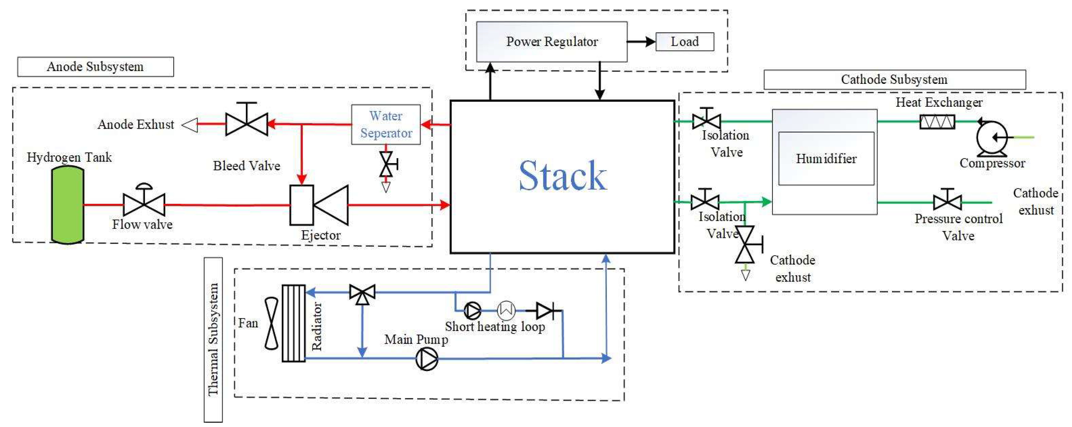
Figure 2.
Ejector schematic model.
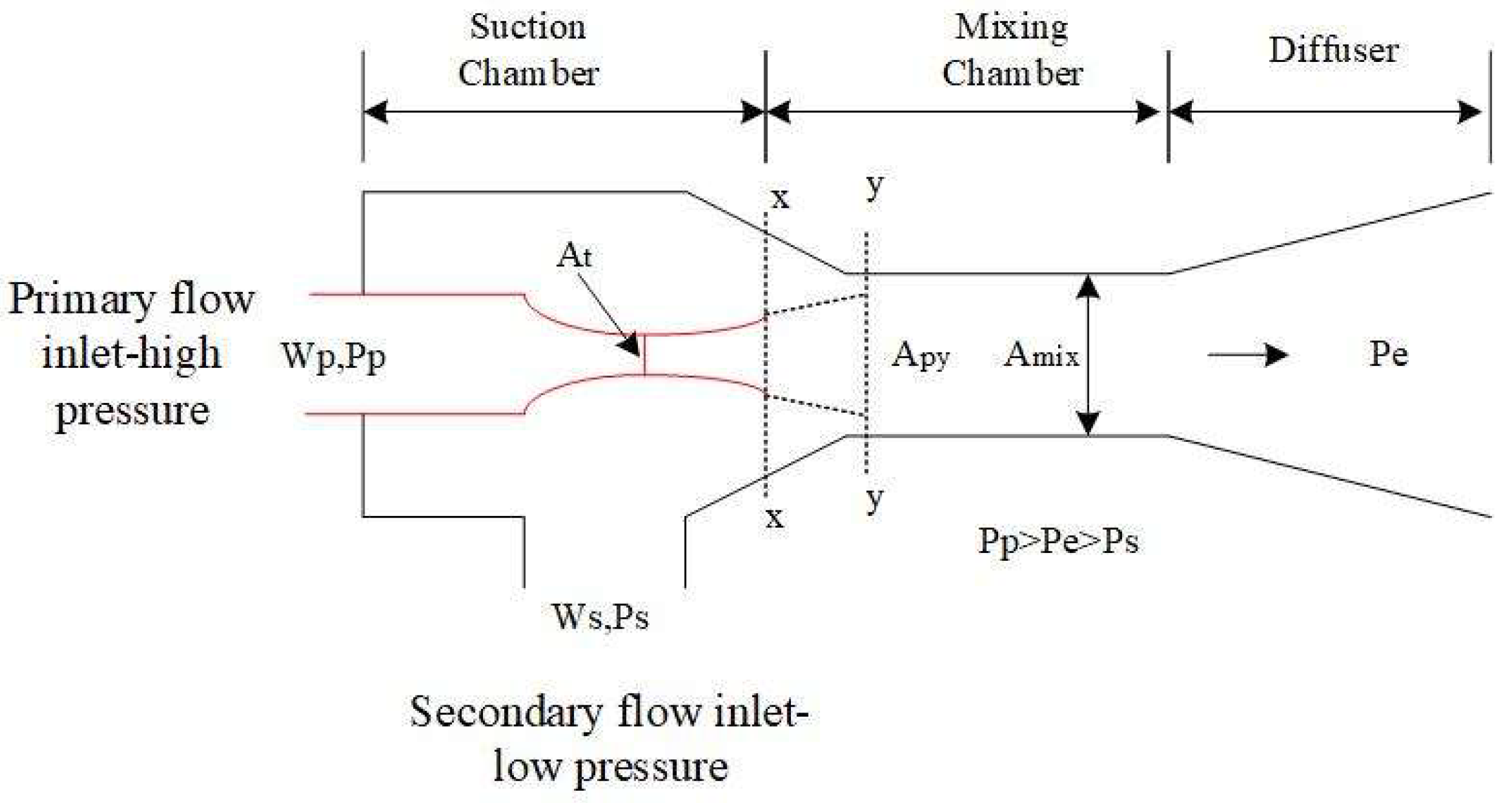
Figure 3.
Offline maps of the optimal operating conditions over appropriate load current range.
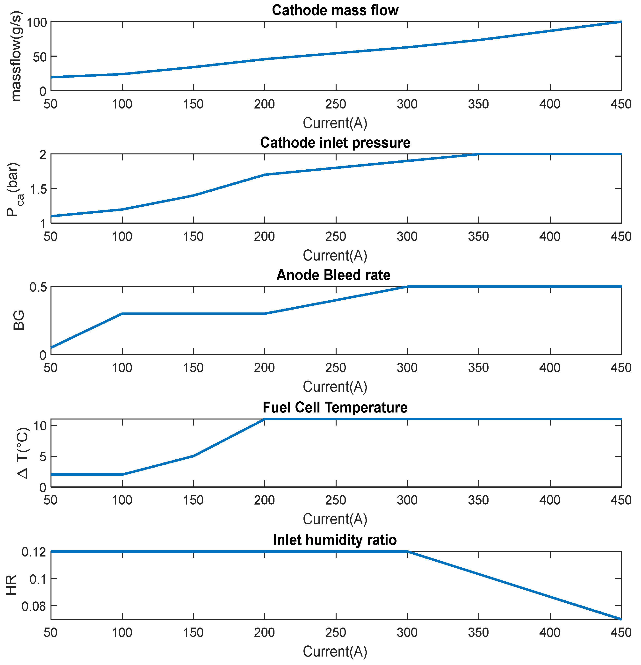
Figure 4.
Upper and lower achievable temperature range of stack.
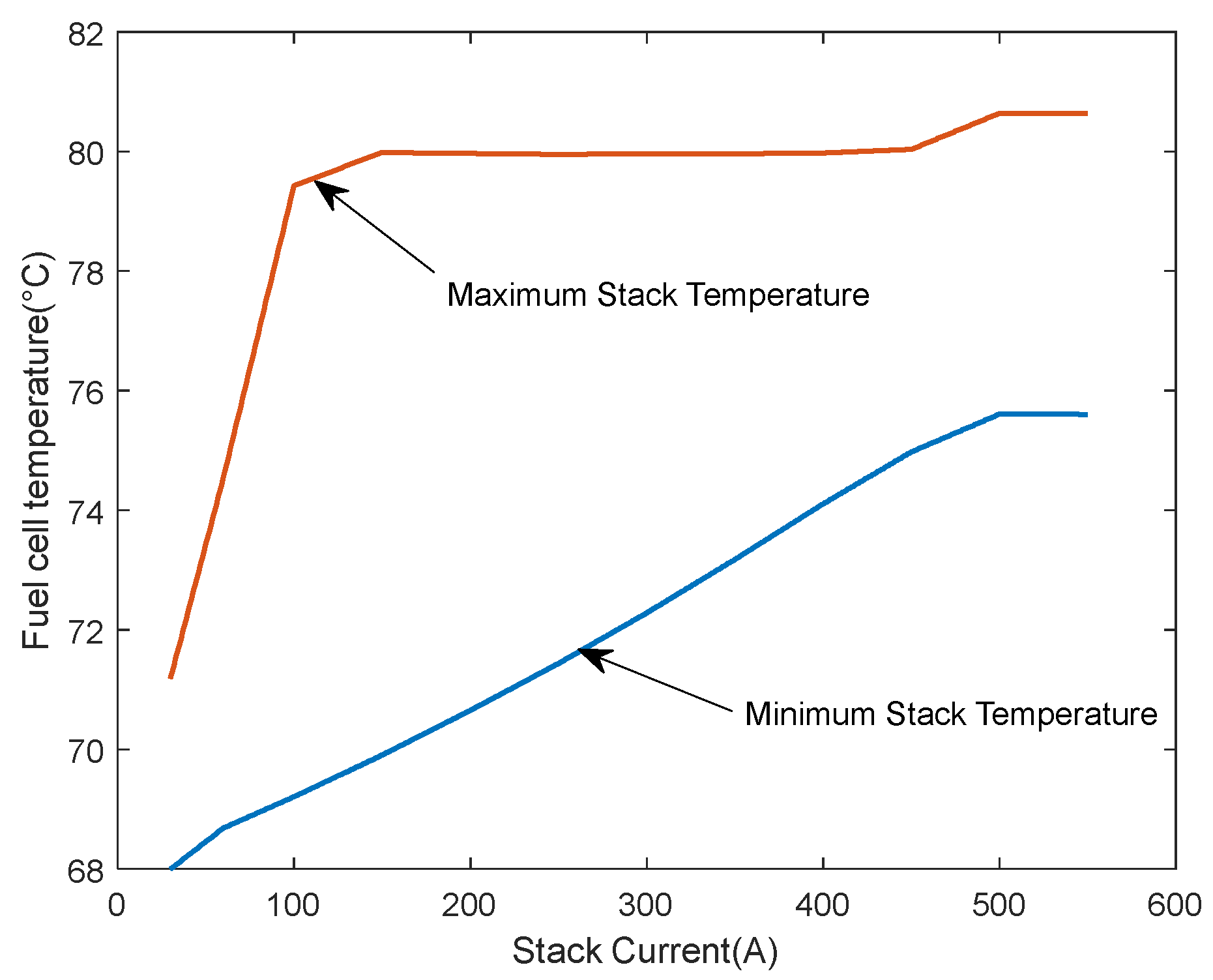
Figure 5.
Proposed MPC control block diagram.
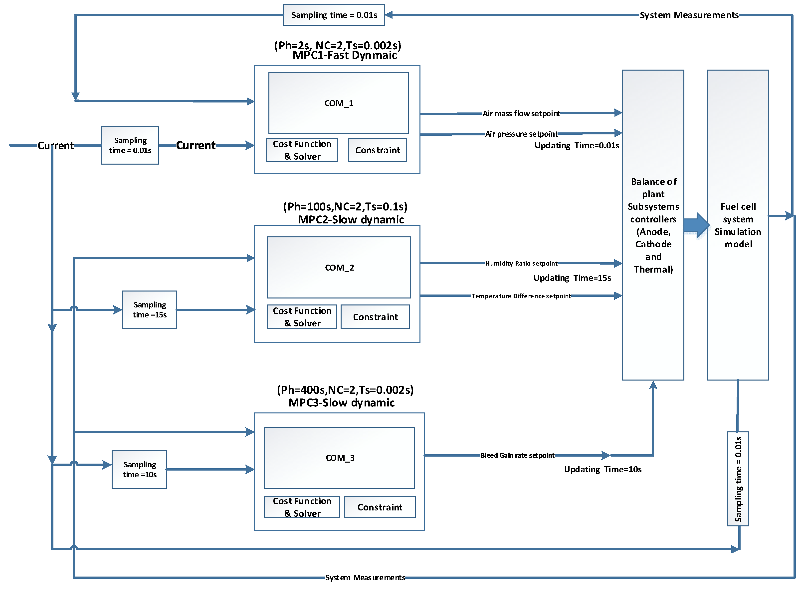
Figure 6.
Behavior of partial pressure of gas species in the anode channel and the system efficiency when the bleed gain changes.
Figure 6.
Behavior of partial pressure of gas species in the anode channel and the system efficiency when the bleed gain changes.
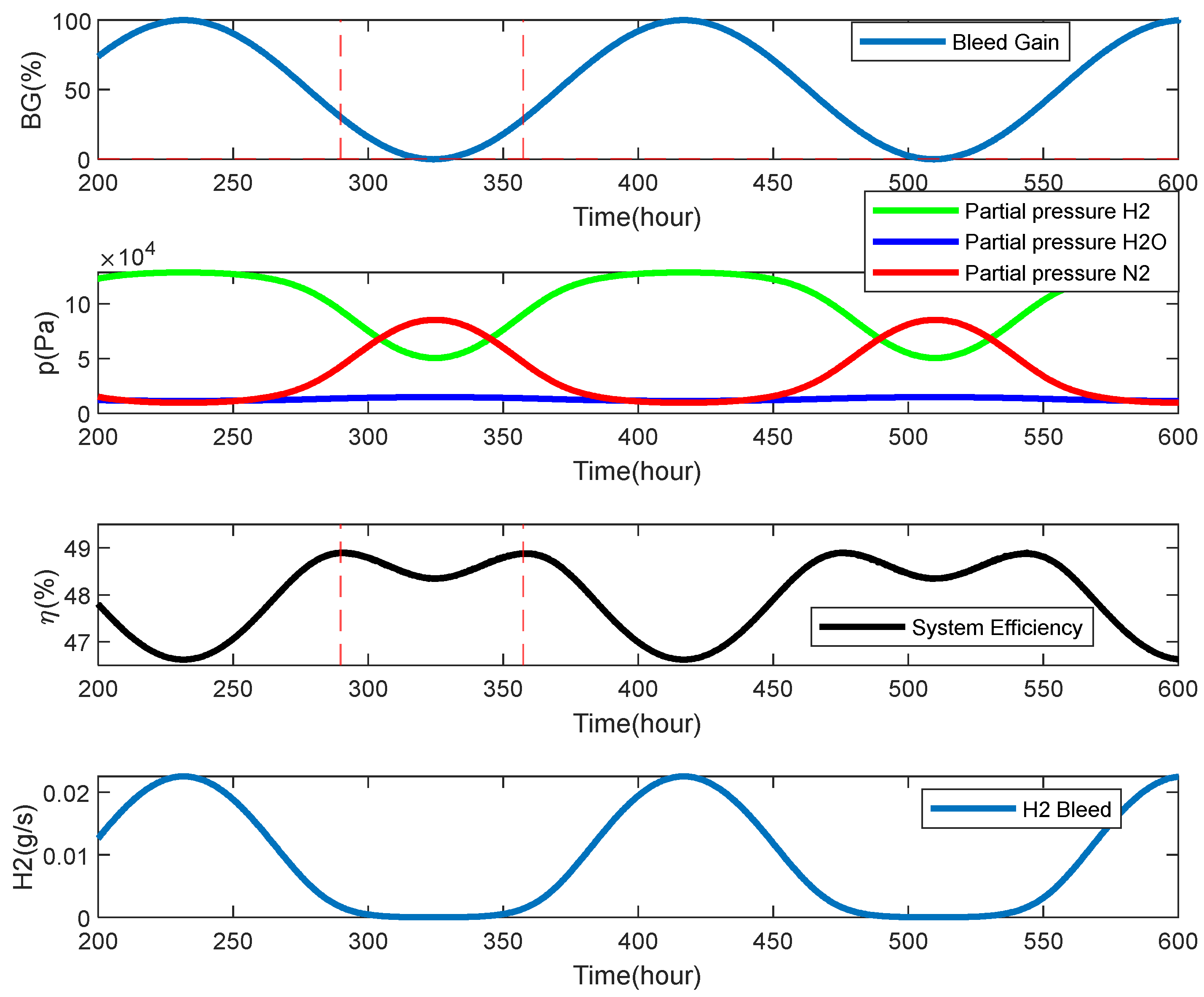
Figure 7.
Generated air mass flow rate and pressure setpoints corresponding the dynamic load current.
Figure 7.
Generated air mass flow rate and pressure setpoints corresponding the dynamic load current.
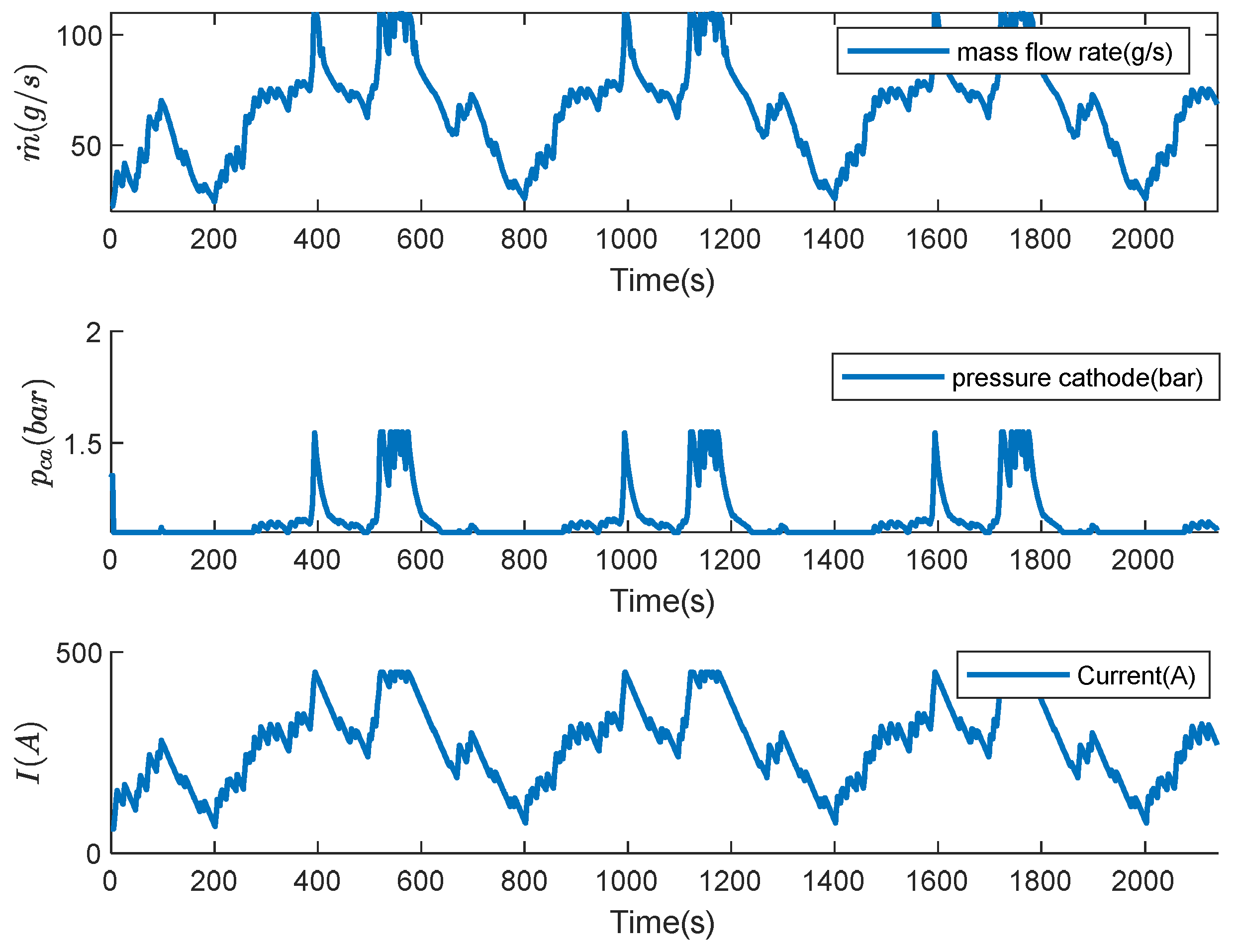
Figure 8.
Generated setpoints for bleed gain rate, humidity ratio, and temperature difference correspond to the dynamic load current.
Figure 8.
Generated setpoints for bleed gain rate, humidity ratio, and temperature difference correspond to the dynamic load current.
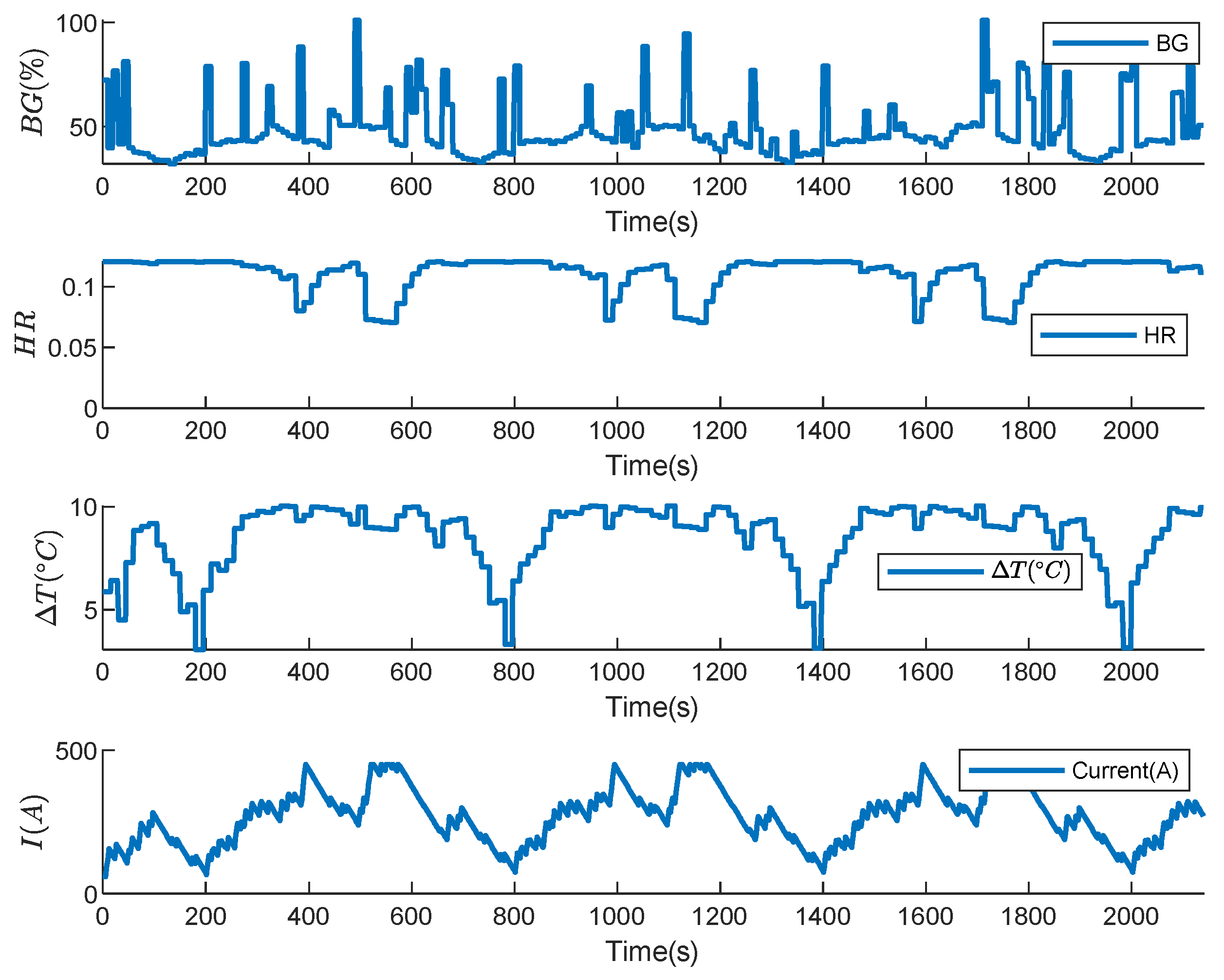
Figure 9.
System average efficiency comparison between the offline setpoint generator and MPC.
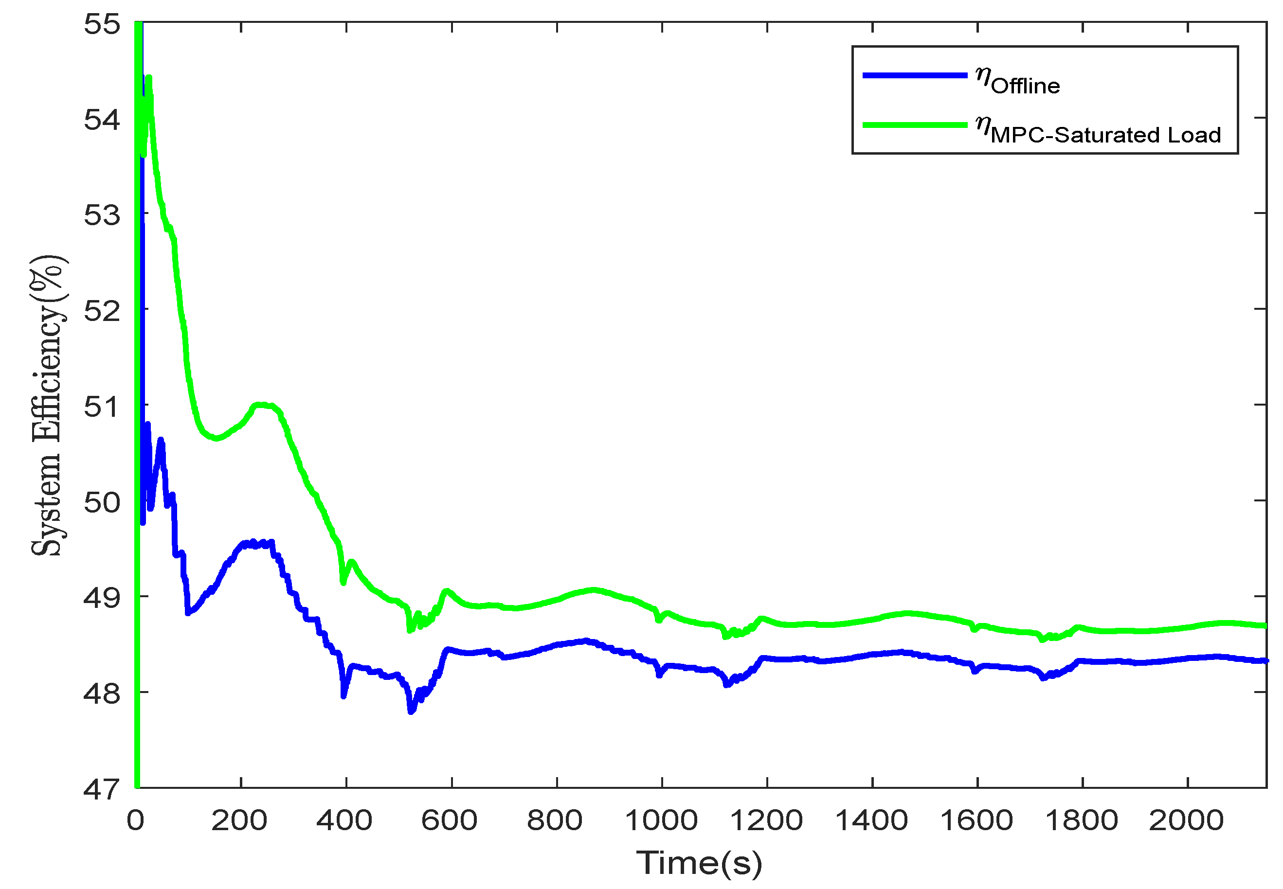
Figure 10.
System average efficiency comparison between the offline setpoint generator and MPC, where one scenario involves knowing the load current beforehand, and the other scenario involves knowing the current for only 5 seconds and assuming a constant load current after that period.
Figure 10.
System average efficiency comparison between the offline setpoint generator and MPC, where one scenario involves knowing the load current beforehand, and the other scenario involves knowing the current for only 5 seconds and assuming a constant load current after that period.
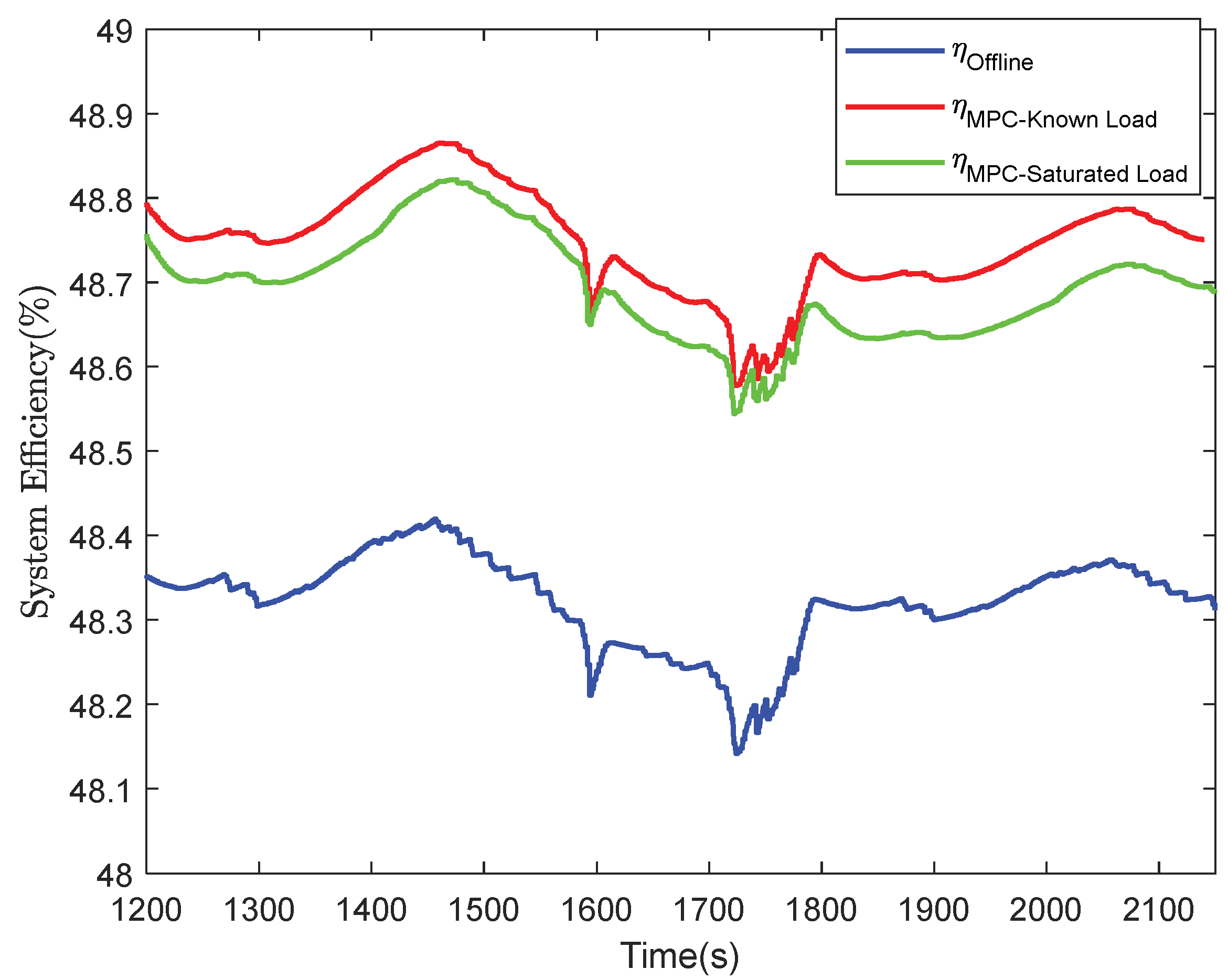

Table 1.
Characteristics of the proposed Model predictive controllers.
| MPC type | Updating sampling time ) | ) | Computation time (s) | Setpoints | ) | COMs Sampling time () |
| MPC-Fast | 0.01 second | 2 second | [.30 1.5] | 2 second | 0.01 | |
| MPC-Slow | 15 second | 100 second | ~10 | 5 second | 0.1 | |
| MPC-Bleed | 10 second | 400 second | ~60 | 5 second | 0.01 |
Disclaimer/Publisher’s Note: The statements, opinions and data contained in all publications are solely those of the individual author(s) and contributor(s) and not of MDPI and/or the editor(s). MDPI and/or the editor(s) disclaim responsibility for any injury to people or property resulting from any ideas, methods, instructions or products referred to in the content. |
© 2026 by the authors. Licensee MDPI, Basel, Switzerland. This article is an open access article distributed under the terms and conditions of the Creative Commons Attribution (CC BY) license (http://creativecommons.org/licenses/by/4.0/).
Copyright: This open access article is published under a Creative Commons CC BY 4.0 license, which permit the free download, distribution, and reuse, provided that the author and preprint are cited in any reuse.