

Submitted:
11 September 2026
Posted:
14 September 2026
You are already at the latest version
Abstract
Systems procured as digital twins of water networks are widely promoted for municipal use, yet evidence on whether they close the chain from sensor to decision in small utilities is scarce. We report a comparative operational audit of three publicly funded Internet of Things (IoT) deployments in Greek water utilities: Argos–Mycenae, Aigialeia and Souli. Using a harmonised twelve-month window and an explicit 0–4 rubric, we scored five sequential layers—sensing, transmission, data management, modelling and decision integration—and recomputed the utilities’ regulatory loss indicators. Modelling was never chain-limiting, but only one case evidenced a calibration. Data management was chain-limiting in all three cases and transmission in two: the Souli archive holds 240 one-minute records, 53 of 119 channels do not vary, and the tags needed to interpret that are absent; the Aigialeia daily series reaches 96.9% completeness but only 48 h are sub-hourly. Documentary decision traceability was level 1 throughout, bounded by the retrieval scope. The outcome holds under four alternative windows, and the statutory reporting artefacts disagree by 3.6% on real losses. The constraint is data stewardship rather than instrumentation, so the layer test transfers to other instrumented urban services.
Keywords:
water distribution networks
; Internet of Things
; operational audit
; data quality
; telemetry
; leakage
; water quality monitoring
; small utilities
; capability maturity
; smart water governance
1. Introduction
Municipal water digitalisation is usually described as a sequence: instrument the network, transmit the readings, store them, couple them to a calibrated hydraulic model, and let the resulting system drive operational decisions. Grigg traces this arc through the sector and notes that adoption is constrained less by technology availability than by return-on-investment uncertainty, workforce capacity and legacy-system retrofit [1].
The empirical record supports the sequence less firmly than the narrative implies. Azadi et al., reviewing 88 urban digital twin studies, report that most contributions are technical and few are embedded in a planning or decision process [2]. Zuñiga-Uribe et al., across 53 artificial-intelligence leak-detection studies published between 2018 and 2025, find heavy reliance on EPANET-generated synthetic scenarios rather than field measurement [3]. Rajan and Li reach a similar conclusion from the flow-data side, separating detection as a research problem from management as an operational one [4]. Ghorbani Bam et al., surveying 147 water-sector digital twin applications, note that small-utility deployments are largely absent [5]. Berg and Marques, reviewing 190 quantitative utility studies, observe that the benchmarking literature rarely interrogates the quality of its own inputs [6].
This matters because small utilities are numerous. In Greece, water supply is delivered by municipal enterprises (DEYA) and by municipalities operating their own networks; the three examined here serve between 7,019 and 42,000 connections. Mashau et al. identify readiness constraints for small and rural municipalities that do not scale down from metropolitan experience [7], Grigg places financing and organisational integration rather than instrumentation cost at the centre of adoption [8], and Esteban-Narro et al., building an evaluation framework for small and medium-sized cities, find that assessment systems designed for large cities import indicators smaller authorities cannot populate [9]. Correia et al. show the same asymmetry at European scale, with activity concentrated in a small number of large agglomerations [10]. Bell et al. link technical, managerial and financial capacity to operational performance across United States drinking-water systems [11].
Between 2021 and 2024 the EEA and Norway Grants “Water Management” programme financed three thematically aligned Greek projects—SMILE (Argos–Mycenae), SWAN (Aigialeia) and SMASH (Souli)—each pairing a utility with a university, each structured around a similar sequence of deliverables, and each specifying a three-tier IoT platform with comparable communication requirements [12]. The three utilities differ in scale, terrain, source mix and network density while sharing an institutional and technical template. They therefore permit a comparative multiple-case study in the sense of Yin [13] and Eisenhardt [14]: purposively selected cases, examined under a common protocol, compared for cross-case patterns. We are explicit that this is not an experimental or quasi-experimental design. There is no exogenous assignment, no common measurement procedure imposed at the time of installation, and—as Section 3.2 shows—no shared period of observation.
Prior work by the present authors has reported on individual elements of these deployments: the integrated leakage-detection platform for Aigio [15], the smart control system for Paramythia in the Souli network [16], and remote-sensing-based leakage monitoring in the Nestos area [17]; and, separately, on carbon accounting for municipal water infrastructure [18,19]. What has not been attempted is a layer-by-layer audit of whether these deployments close the loop from sensor to decision.
The question generalises beyond water. A water network is one of several urban services—mobility, waste collection, street lighting, building energy, environmental monitoring—now procured as instrumented systems on the same premise, that measurement will propagate into operation. Each is delivered through the same five stages, and each is assembled from the same municipal capacity: the technical staff, the procurement instrument and the data-stewardship arrangements of a single local authority. If the chain breaks at a common stage in one service, that stage is a candidate constraint in the others, because what fails there is not domain-specific technology. We examine water because it is the domain in which audit evidence could be assembled; Section 4.3 sets out what the result implies for urban operations more broadly, and on what basis that transfer can and cannot be claimed.
That is the contribution here. We argue that the appropriate unit of assessment is not the presence of a platform but the integrity of the chain feeding it—consistent with Mousavi et al.’s distinction between digital model, digital shadow and digital twin [20] and with the ingestion concerns set out by Osolinskyi et al. [21]—and that this chain can be scored against explicit criteria. Three questions follow:
- RQ1. Under a common audit protocol, how do the three utilities differ across the five layers of the sensor-to-decision chain?
- RQ2. Where is the binding constraint, and how robust is its location to alternative scoring assumptions?
- RQ3. What do the retrievable archives and the utilities’ regulatory submissions support in the way of leakage and water-quality conclusions, and how sensitive are those conclusions to the source used?
2. Materials and Methods
2.1. Research Design
The study is a comparative multiple-case operational audit. Three deployments were purposively selected because they share a funding instrument, a deliverable structure and a platform specification while differing in the physical characteristics that plausibly condition digitalisation outcomes. They are not a representative or exhaustive sample of Greek water systems, and no claim of statistical generalisation is made; the intended inference is analytical, in Yin’s sense [13].
Figure 1 sets out the design. Four evidence streams feed a documented retrieval protocol; the retrieved material is subjected to five archive-level tests and four channel-level diagnostics; the results are scored against a published rubric and compared across cases. A harmonised twelve-month reference window supports the cross-case coverage statistics, and its selection and sensitivity are set out in Section 2.4.
2.2. Study Areas
2.3. The Three Deployments
All three projects were financed under the EEA Financial Mechanism 2014–2021 “Water Management” programme, which targets leak detection through IoT and telemetry [12]. Table 2 sets out their technical configuration as documented in the project deliverables; the Supplementary Material reproduces the full deliverable list and the retrieval log.
Three features deserve note. The communication specifications for Argos and Aigialeia are written as a menu of options rather than a committed choice, which defers the interoperability decision to the operating phase—the risk that Ntafalias et al. address architecturally [22] and that Villar Miguelez et al. treat as a security and lifecycle commitment rather than a procurement option [23]. Only Souli instruments water quality, notwithstanding project framing that references quality monitoring in all three. And only Argos documents a live coupling between sensor database and hydraulic model, the feature that in Mousavi et al.’s taxonomy separates a digital twin from a digital shadow [20] and that Ciliberti et al. use to separate a hydraulic model from a digital water service [24].
2.4. Reference Window and Archive-Audit Protocol
The reviewer-facing weakness of an audit like this is that archives of different length, resolution and vintage are not directly comparable. We address it in two ways.
First, a harmonised reference window of twelve months, 1 May 2025 to 30 April 2026, anchors the cross-case coverage statistics.
We are explicit about its provenance, because it bears on how much weight the statistic can carry. The window was not declared in advance. The archives were examined first, and the window was fixed afterwards, during the re-analysis that produced this version of the study. It is therefore a post hoc harmonised window, not a prospectively registered one, and it cannot be presented as a pre-specified design element.
The selection rule was stated before the candidates were compared and is deliberately generous to the deployments: of all twelve-month periods, this is the only one containing both sub-hourly telemetry from one of the three cases and a complete annual record from one of them. Choosing the window most favourable to the systems under audit guards against the obvious hazard of a post hoc choice, which is that the analyst picks the period that flatters the argument.
Because a post hoc window invites exactly that suspicion, Section 3.8 reports the transmission-layer scores and the chain-limited level under four candidate windows: the harmonised window; the twelve months to 31 October 2023, which contains the longest continuous daily series together with a sub-hourly block; the twelve months to 30 September 2023, which maximises coverage of that daily series; and the twelve months to 31 July 2026, the most recent complete twelve months before the audit. The conclusions do not depend on the choice.
Coverage is reported against the window and, separately, against each archive’s own span; the two are never combined into a single figure. Where an archive predates the window, its transmission score is assessed over an equivalent twelve-month period ending at its last timestamp, so that an older archive is not penalised for its vintage; Section 3.8 shows what happens when that allowance is withdrawn.
Second, archive quality is decomposed into five distinct tests rather than a single completeness percentage, because a single percentage conflates conditions that call for different remedies:
- 3.
- Archive availability—does a machine-readable archive exist for the deployment?
- 4.
- Window coverage—does any part of it fall inside the reference window?
- 5.
- Within-span completeness—observed records as a fraction of records expected at the archive’s own nominal interval over its own first-to-last timestamp.
- 6.
- Continuity—the number, length and distribution of gaps, reported explicitly rather than folded into a percentage.
- 7.
- Retrievability—was the archive supplied, in machine-readable form, in response to a request issued before the audit cut-off?
An archive that is not supplied is recorded as not assessable on tests 2–4, not as zero. We use “not supplied by the audit cut-off” rather than “cannot be retrieved” throughout: the audit establishes that an archive did not arrive, not that it does not exist or could not be produced given longer. Section 4.5 records the response window as a limitation, and Section 3.8 shows that the conclusions are unchanged if the Argos archive is assumed to exist in full. This distinction matters: zero is a measurement, not-assessable is its absence, and treating the second as the first would overstate what we know.
At channel level, four further diagnostics were applied to the multivariate exports: classification of each channel as varying, constant-zero or constant-non-zero; screening for physically implausible or non-finite values; a check of whether stored values fall within the plausible engineering range for the declared measurand; and completeness of the instrument metadata register.
On the interpretation of constant-zero channels we are deliberately cautious. A channel may read zero because the sensor has failed, because the plant it monitors was idle, because zero is a legitimate value, or because the sampling window was too short to capture variation. Distinguishing these requires station heartbeat, communication status or operating logs. Section 3.3 reports what the exports do and do not contain in this respect. Throughout, we therefore use the descriptive term non-varying and reserve any inference about sensor failure to cases where corroborating evidence exists.
2.5. The Sensor-to-Decision Capability Maturity Model
Smart-city assessment instruments are numerous, and Patrão et al. find them weighted toward static technology-presence indicators [25]. Maturity models fit the present question better: Aljowder et al.’s focus-area model supplies the structure [26], Angelakoglou et al.’s indicator-selection method informs the choice of measurable proxies [27], Lafioune et al. provide a municipal digital-transformation maturity framework from outside the smart-city literature [28], and Lawrence’s data readiness levels supply the underlying idea that data must be graded on accessibility before it can be graded on fitness for purpose [29]. The dimensions themselves follow ISO/IEC 25012 [30], and the link between data-quality management and organisational process capability follows ISO 8000-61 [31]; stewardship roles follow DAMA-DMBOK [32] and the metadata expectations follow the FAIR principles [33].
The Sensor-to-Decision Capability Maturity Model (S2D-CMM) comprises five sequential layers scored 0–4 against the explicit criteria in Table 3. The criteria are stated in terms that can be checked against documents or data, so that a third party with the same material should arrive at the same score.
Three definitions and qualifications attach to the rubric and are applied uniformly.
The positive-evidence rule: a level is awarded only where every condition for it is positively evidenced in the retrieved material. Absence of evidence therefore maps downward, to the highest level that is positively evidenced, and never upward. This is why Argos–Mycenae scores 1 rather than 2 at the data-management layer: its sensor-to-asset mapping is documented, which is one of the level-2 conditions, but schema stability cannot be assessed because no archive was supplied, so level 2 is not fully evidenced. The rule is deliberately conservative and is applied uniformly; where it produces a score that the documentation alone might have supported, the item is marked † in Table 4 and the alternative is carried through the sensitivity analysis.
A monitoring point is a physical location at which at least one process variable is instrumented and telemetered—a station, not a sensor and not a measurement channel. Souli’s 19 stations carry 1,347 I/O points between them; the density figures below count the 19, and channel counts are reported separately wherever they matter.
The L1 levels are cumulative on density: a deployment cannot reach level 3 on parameter breadth alone if its density falls below the level-2 band. Water-quality breadth is a qualifier applied on top of the density requirement, not a substitute for it.
The L1 coverage cap: density is assessed within the instrumented zone, but a deployment covering less than 10% of the utility’s service connections cannot be scored above level 2, because a capability confined to a small pilot is not a utility capability. This is what separates Aigialeia, whose single point serves a zone of 973 meters at nominally high density but only 2.3% of the utility, from Souli, whose stations serve the whole municipality.
The L2 assessment period: coverage is computed over the harmonised window where the archive falls inside it, and over an equivalent twelve-month period ending at the archive’s last timestamp where it does not, so that an older archive is not penalised for its vintage. This allowance is the most favourable treatment available to each archive; Section 3.8 reports what the scores become without it. Resolution is treated as a distinct axis because it determines what the record can be used for: sub-hourly data supports minimum-night-flow and burst detection, daily data supports water balance and trend detection, and monthly data supports accounting only. A monthly record therefore cannot reach level 2 however complete it is.
Two summary statistics are reported. The capability profile is the vector of five layer scores. The chain-limited level is the minimum across the five, and expresses the capability actually available to a decision, on the reasoning that a serial chain cannot deliver more than its weakest stage: a calibrated model fed no data produces no decision.
We deliberately do not convert the five ordinal scores into a single index on a 0–100 scale. Ordinal levels are not equally spaced and are not additive in any measurement-theoretic sense, and rescaling them imputes a precision the instrument does not have. No summed score is reported anywhere in this paper.
2.6. Scoring Procedure, Agreement and Sensitivity
Scoring was performed independently by two of the authors against the Table 3 criteria and the retrieved evidence, then reconciled. Percentage agreement before reconciliation was 13 of 15 layer scores (86.7%); both disagreements were by one level, on Argos L3 and Souli L5, and both were resolved by adopting the lower score. With fifteen items on a five-point scale a weighted kappa estimate would be unstable, so we report raw agreement and treat the reconciled scores as provisional. Table S1 records the specific evidence behind each score.
Both of those scorers had project involvement (Section 6), which makes the scoring circular in an important respect: the instrument was applied only by people associated with the systems it assesses.
To address this, a blind re-scoring protocol was specified in advance and is reproduced in full in the Supplementary Material (Table S8): the author with no involvement in any of the three deployments scores all fifteen items from the Table 3 rubric and the retrieved artefacts, without sight of Table S1, of the reconciled scores, of the figures or of any draft of the results; agreement is then reported item by item as exact matches and matches within one level; and where a blind score differs from the reconciled score, both are reported and the lower is adopted, consistent with the reconciliation rule applied between the first two scorers.
Table S1 carries a column for the blind scores. At the time of writing that pass has been specified but not executed, and the column is empty; the reconciled scores of the two involved raters are the only scores this version reports. A blind pass by a co-author would in any case not be equivalent to assessment by a rater external to the author team, which remains the appropriate standard for any use of the instrument beyond these three cases.
Two of the four authors were professionally involved in the deployments assessed (Section 6). This is a material limitation for a scoring exercise, and we address it in three ways: by publishing the rubric so that scores can be challenged item by item; by publishing the underlying evidence for each score; and by reporting three robustness checks (Section 3.8): a capability-threshold requirements analysis, a variation of the two contested scores across the range the scorers proposed, and a reference-window sensitivity analysis. An independent re-scoring by a rater with no involvement in the projects is the appropriate next step and has not yet been performed.
2.7. Recomputation of Regulatory Indicators
Each utility’s water audit was recomputed rather than transcribed. Volumes were taken from the Β4 statutory balance tables and the WB-EasyCalc v6.17 workbooks; performance indicators follow IWA definitions [34,35], with data-validity considerations following the AWWA water-audit methodology [36]. Unavoidable annual real losses were decomposed into their three constituent terms to establish how much of each utility’s allowance derives from mains length as opposed to connection count. Energy attributable to water supply was isolated from total municipal electricity consumption at the level of individual supply accounts, following the allocation procedure established in our earlier work [18], and organisational emissions follow ISO 14064-1 [37].
Where the sources disagree we report the disagreement rather than selecting one. Section 3.9 gives the resulting ranges.
2.8. Software and Reproducibility
Extraction of the primary artefacts used Python 3.11.2 with pandas 2.2.3 and openpyxl 3.1.5. The analysis and figure scripts supplied as Code S1 require only matplotlib 3.10.9 and numpy 2.4.4. Every numeric quantity plotted in Figure 2 to 10 is read from Dataset S1 rather than held in the plotting code, and figures.py reproduces the ten submitted figures byte for byte; verify_package.py performs that comparison, together with checks on wording, numbering, dataset integrity and the package manifest. The processing code, the derived indicator dataset, the scoring matrix with per-item evidence and the retrieval log are provided as Supplementary Material. The primary telemetry archives and regulatory submissions are the property of the respective utilities and are available from them subject to authorisation; the derived dataset contains no confidential material.
3. Results
Figure 3 summarises the layer-by-layer outcome for the three deployments; the sections that follow give the evidence.
3.1. Sensing
Instrumentation density differs by an order of magnitude, and not in proportion to network size. Argos–Mycenae operates two pre-existing supervisory flow and pressure points in a pilot zone containing 11,496 active meters, with seven further sensors specified; on evidenced instrumentation this is one point per 5,748 connections. Aigialeia operates one inlet point serving 973 meters in district metered area 27, with four further sensors specified—one point per 973 connections, the highest density of the three, achieved by defining a small zone rather than by dense instrumentation. Souli’s I/O list documents 19 remote stations comprising 1,347 individual I/O points across 7,019 connections, roughly one station per 369 connections.
Station inventories are not consistent across the Souli documentation, and this is itself a finding. The process and instrumentation diagram covers 29 stations (12 supply and 17 pumping or treatment); the I/O list covers 19; the data export schema carries 21 station prefixes, of which one (TSE011) is a naming error for TSE11, giving 20. No document reconciles the three. An analyst asking how many stations exist would obtain three different answers depending on which artefact was consulted.
Parameter breadth separates the cases more sharply than density. Both DEYA deployments instrument flow and pressure only. Souli instruments residual chlorine and pH at nine stations and adds turbidity and conductivity at four (TSE05, TSE11, TSEE01, TSEE03). Souli also instruments actuation, with 439 variable-frequency-drive signals and 128 automatic chlorination dosing signals, and is therefore the only one of the three capable in principle of closing a control loop rather than observing.
None of the three derived its instrumentation layout from a formal sensor-placement optimisation; positions followed existing valve boundaries and available power supply. Gamboa-Medina and Reis show that sampling design materially affects detectability for a given sensor count [38], and Piazza et al. demonstrate the same for quality-sensor placement under alternative quality models [39]. Applying Table 3, Argos–Mycenae reaches the density band for level 2 and covers 46% of the utility’s connections; Aigialeia reaches the density band for level 3 within its zone but covers 2.3% of the utility and is therefore capped at level 2; Souli reaches the density band for level 3 and instruments the whole municipality, and adds four quality parameters. L1 scores are 2, 2 and 3 respectively.
3.2. Archive Availability, Coverage and Continuity
Figure 5 states the comparability problem plainly. The Aigialeia sub-hourly record is a 48-hour block in October 2023; the Souli sub-hourly record is five hours across two days in June and July 2025, twenty-eight days apart; the Argos archive was not supplied by the audit cut-off. There is no period in which the three can be compared at operational resolution, and any statistic that implies otherwise would be an artefact of construction rather than a finding. This is why the audit reports the five tests separately.
Within the reference window, the Souli one-minute export contributes 240 multivariate records—the 13 June 2025 file carries only three variables of a single station and is excluded from the multivariate count—against approximately 525,600 minute-slots, and the field logger contributes eight records. The Souli monthly aggregation workbook, by contrast, covers the reference window exactly, twelve months of twelve, and is the only archive in the study that does. Aigialeia’s daily series is the most continuous record in the study, 618 of 638 days from 24 December 2021 to 22 September 2023, a within-span completeness of 96.9%, with 20 absent days distributed across 14 gaps of which twelve are one or two days and two are three days. It is, however, entirely outside the reference window and at daily resolution, which is too coarse for the minimum-night-flow methods that dominate real-loss estimation practice [40,41,42]. Within the 48-hour high-resolution block the data are clean and usable: the cumulative supply meter advances from 946,237 to 947,133 m³, giving 896 m³ over two days for the zone, at an inlet pressure stable between 4.13 and 4.15 bar.
The 2019 Aigialeia monthly reports require a correction to the record. Their tag naming (Τ.Σ.Ε., Υ.Τ.Σ.Ε., Σ.Ε.Δ. with Greek abbreviations and full stops), their code pages (CP1253 and ISO-8859-7) and their dates all predate the SWAN project by two years. They are exports from the utility’s pre-existing supervisory system, and the defects they contain are properly attributed to that system, not to the project. Those defects are nonetheless instructive: the column header count rises from 23 to 33 to 62 to 63 across the year as stations are commissioned; February 2019 contains only a header; May 2019 is absent; the data rows do not match their own headers, with field counts of 62, 63, 64 and 66 occurring inside a single file; and 36 negative flow values are stored without flag or correction, the largest being −475,252.53 and −455,262.50 at station Τ.Σ.Ε.08. Three different character encodings appear across the eleven Aigialeia files retrieved, of which seven are the 2019 monthly reports. This is the concrete form the ingestion problem takes, and it is the case for the schema validation and unit dictionaries that Osolinskyi et al. place at the ingestion boundary [21].
For Argos–Mycenae, deliverable Π2.6 documents a PostgreSQL instance on a cloud server, a MIKE+ model bound to it, and an explicit mapping of each sensor to its corresponding node, pipe, pump or reservoir. No archive was supplied before the audit cut-off. We record this as non-supply and as not assessable on the remaining tests. The request was issued to the utility’s technical service and the cut-off followed shortly after, which is a short response window and a real weakness of the audit rather than a property of the archive; the sensitivity analysis in Section 3.8 therefore also reports what follows if the archive is assumed to exist and to be complete. L2 scores are 1 (Argos, on non-supply), 2 (Aigialeia) and 1 (Souli).
3.3. Channel Diagnostics
Figure 6.
Channel-level diagnostics for the Souli one-minute export (119 channels, 240 records). (a) Behaviour of each channel over the observation period. (b) Distribution of non-varying channels by station; four stations return no variation on any channel. (c) Diagnostic signals present in the project I/O list against those present in the data export.
Figure 6.
Channel-level diagnostics for the Souli one-minute export (119 channels, 240 records). (a) Behaviour of each channel over the observation period. (b) Distribution of non-varying channels by station; four stations return no variation on any channel. (c) Diagnostic signals present in the project I/O list against those present in the data export.
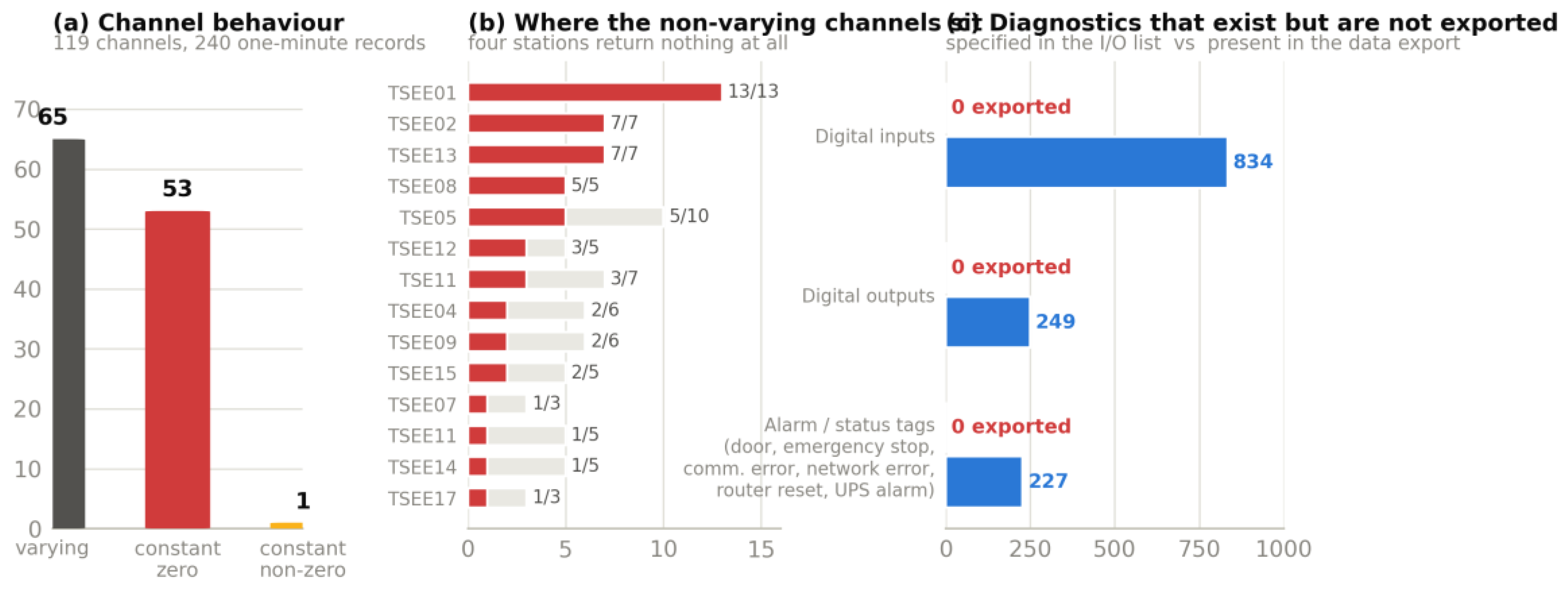
Of the 119 channels in the Souli export schema, 65 vary over the 240 records, 53 are constant at zero, and one (TSEE15_FT01) is constant at a non-zero value of 100.0. No channel has missing values; every channel carries 240 of 240 readings, which indicates that the export pipeline itself was functioning throughout.
The concentration of the non-varying channels is informative. Four stations—TSEE01 (all 13 channels), TSEE02 (all 7), TSEE13 (all 7) and TSEE08 (all 5)—return no variation on any channel, accounting for 32 of the 53. A further 21 are isolated channels at eight other stations, most often the active-power channel.
Whether these represent failed instrumentation cannot be established from the export, and we do not claim that it can. A four-hour window is short; a pump that did not run during it will report zero power legitimately. What can be established is that the export makes the question unanswerable. The 119-channel schema contains only analogue measurands—flow, pressure, level, active power and the four quality parameters—and no digital, status or heartbeat signal whatsoever; a regex search of the header for communication-error, network-error, router-reset, door, emergency-stop, alarm, fault and status patterns returns nothing. The corresponding signals exist in the project I/O list, which specifies 834 digital inputs, 249 digital outputs and 227 tags of alarm or status type, including 19 communication-error, 19 network-error and 19 router-reset tags. None is exported. The diagnostic information required to interpret a zero is specified in the project I/O list and absent from the data export we were given. Whether every listed tag was ultimately wired and commissioned is not something the I/O list alone establishes, and we did not verify it in the field; nor can we establish that this export is the only artefact available to an analyst, only that it is the one the audit received. This is a data-product design failure rather than an instrumentation failure, and it is the more consequential of the two because it is invisible: a dead channel and an idle pump are indistinguishable in the file.
Two further defects appeared. TSEE16_ACT_POW contains nine non-finite (inf) values among its 240 readings, with the remainder spanning 9.17 × 10⁻³⁶ to 20.6; TSEE16_FT01 has a minimum of 1.58 × 10⁻³⁶. Denormal and non-finite floats of this kind are capable of propagating silently through downstream aggregation. The monthly workbook described in Section 3.5 also contains formula errors and all-zero columns, but we did not establish a lineage between the two, and we do not claim that these particular values produced those particular errors. Branisavljević et al. show that without context classification the separation of genuine events from sensor artefacts degrades sharply [43]; Quevedo et al. demonstrate the validation and reconstruction procedures that would ordinarily catch such values before storage [44]; Osman et al. survey the imputation methods that presuppose such screening [45]. None was applied here.
3.4. Water Quality Monitoring
Water quality is instrumented only in Souli, and the retrievable evidence is thin but not empty. Figure 7 reports it.
Twelve of the sixteen quality channels in the supervisory export vary; the four channels at TSEE01 are constant at zero, consistent with that station being wholly non-varying. Variation alone does not make the values usable. Excluding readings of exactly zero—which we treat as non-readings rather than measurements, on the reasoning that a pH of 0.000 is not physically attainable in a drinking-water network, and which affects 2 of the 240 readings at TSE05 and none at TSE11 or TSEE03—the stored pH values span 3.722 to 3.832 across the three reporting stations. That lies outside the admissible range for water intended for human consumption of 6.5 to 9.5 [46]. The field logger, sampling the network two months later, reports pH between 9.48 and 9.50, conductivity between 869 and 878 µS/cm, turbidity between 0.81 and 0.86 NTU and water temperature between 23.8 and 24.6 °C.
What this comparison establishes, and what it does not, needs stating precisely. Three limitations apply. The supervisory sample is from 11 July 2025 and the logger record from 2 and 4 September 2025, so the two are not synchronous. The logger’s position within the network is not documented in the material retrieved, so the two instruments are not demonstrably co-located. And no calibration record exists for the logger either, so it cannot be treated as a reference instrument—only as an independent one.
The defensible conclusion is therefore that the two sources are mutually inconsistent by about 5.7 pH units—pH being logarithmic, a difference of this size is not expressible as a ratio, and it exceeds by a wide margin any plausible spatial or temporal variation within one supply network—and that the inconsistency cannot be resolved from the metadata available. Since the export carries no unit declaration for any tag (Section 3.5), there is no way to establish which source, if either, is in engineering units. A compliance judgement from either would be unsafe. Resolving it would require a synchronous, co-located reference measurement with documented instrument identity and calibration state—the cross-check protocol that Aisopou and Stoianov set out from nine online sensors compared against reference sampling over two and a half years [48].
Two further observations follow from the logger record, both provisional on eight readings. Free chlorine reads exactly zero in all eight, which is either a genuine absence of residual at that point or an unscaled or failed sensor; free-chlorine sensors are known to drift and foul over extended deployment [47], and no calibration record was found for any Souli quality instrument. And the observed pH of 9.48–9.50 sits at the upper parametric limit rather than comfortably inside it. Neither is actionable as it stands; both are grounds for a targeted verification campaign.
The wider point is that the failure here is not an absence of sensors. Souli instrumented four quality parameters at four stations and two at nine, which exceeds what either of the other two cases in this study instrumented. The difficulty is that the values reach the analyst without a unit declaration, without a documented scaling, without calibration records and without a metadata register that would let anyone establish what they represent. Under the WHO water safety plan framework, operational monitoring is precisely the function this instrumentation is meant to serve [49]; Tsitsifli and Tsoukalas identify resourcing and staffing as the recurring obstacles to that function in practice [50]. What we observe is a third obstacle: the data product itself—which values, in which units, with what provenance—was not documented in the retrieved material.
3.5. Data Management
All three deployments specified persistence; none demonstrated stewardship.
Argos was the only case with a documented sensor-to-asset mapping, which is the prerequisite for any state-estimation approach [51]. Because no archive was supplied by the audit cut-off, that mapping could not be verified in operation, and the two scorers disagreed on whether documentary evidence alone supports level 2. The lower score was adopted; the sensitivity analysis in Section 3.8 tests the consequence.
Aigialeia scores 1 on the SWAN-era artefacts alone. The zone exports retrieved for 2021–2023 carry column headers of the form Diagram 1 Time and Diagram 1 ValueY: no measurand, no unit and no station identity travels with the values, so the file is interpretable only by someone who already knows what was exported. No metadata register, validation rule or sensor-to-asset mapping was retrieved for the project platform.
The 2019 defects catalogued in Section 3.2 are not counted against this score. They belong to the utility’s pre-existing supervisory system, and the data lineage between that system and the project platform could not be established from the material retrieved. We report them as context on the environment the project was installed into, and we note that a lineage statement—which system produced which archive, and what was migrated—is itself a data-management deliverable that no case supplied.
Souli scores 1 on three grounds. The instrument description register is an unpopulated template: 119 tags appear as column headers and the description, measurand-type and unit fields are empty for every one of them, so a tag such as TSEE03_CT01 is uninterpretable outside the commissioning team. The monthly aggregation workbook, covering May 2025 to April 2026 with 95 value columns, carries 32 columns that are entirely zero or empty and 60 cells of #VALUE! error concentrated in five columns, so the aggregate layer inherits and propagates the channel failures below it rather than surfacing them. And the non-finite values of Section 3.3 pass through unscreened.
The monthly workbook nonetheless deserves a fairer hearing than the one-minute export. Sixty-three of its 95 columns carry values, including eleven of the seventeen station power columns, and it covers the reference window completely. It is a usable, if unvalidated, monthly record. The claim that these utilities produce no usable telemetry would be too strong; the accurate claim is that they produce no telemetry at a resolution or with a provenance that supports leak localisation.
3.6. Modelling
Hydraulic modelling is never the chain-limiting layer, and at Argos–Mycenae it is the highest-scoring layer of the five. It is not uniformly the strongest: at Aigialeia it ties with sensing and transmission at 2, and at Souli it sits one level below sensing. The finding worth stating is narrower than “modelling is strong”—it is that model capability binds none of these systems, while only one of the three evidenced a calibration.
Argos scores 3. Deliverable Π2.1 documents a MIKE+ model of district metered area 1 built on geocoded consumption records for 2013–2015 and 2020/2022, disaggregated from six-monthly billing to daily and hourly demand, over elevations from a digital elevation model spanning 2–76 m. Π2.2 documents calibration against a supervisory demand pattern and simulation of paired scenarios with and without leakage, which satisfies the level-3 requirement that the calibration source and period be documented. Goodness-of-fit statistics were not reported in the material retrieved, and the score should be read with that qualification. Π2.6 documents an online coupling to the sensor database and a deviation-flagging logic in which a baseline model is run against live measurement—the canonical model-based architecture [52,53]—but level 4 requires evidence of that binding in operation, and with no archive supplied by the audit cut-off no such evidence was available. Argos is therefore the only case with a documented calibration and the only case whose live binding is documented but unevidenced.
Aigialeia scores 2. A MIKE+ model of district metered area 27 on an EPANET 2.0 engine is documented, together with a three-view web application covering hydrometers, supply meters and electricity meters. The inclusion of electricity meters in the visualisation layer is uncommon in the Greek municipal deployments we have examined and is the interface through which a water–energy analysis would be conducted. No calibration dataset, calibration period or fit statistic was retrieved, which caps the score at level 2 under the revised rubric.
Souli scores 2 on the same ground. The Paramythia model is well specified, and the decision-support specification sets out a coherent indicator logic based on the IWA balance and the standard performance-indicator set [34,35], inferring leakage by comparing modelled ideal operation against sensor values. No calibration evidence was retrieved.
The distinction the revised rubric draws—between a model that has been built, one that has been calibrated, and one that is bound to live data in operation—matters because the three are routinely conflated in project reporting. On the evidence retrieved, all three cases have built models, one has a documented calibration, and none has an evidenced live binding.
3.7. Decision Integration
No decision traceability was identified in the artefact set retrieved for this audit. That is the claim the evidence supports, and it is weaker than the claim that no such decisions were taken.
The distinction matters. Our retrieval covered project deliverables, telemetry archives, regulatory submissions and the platform documentation, and in that material decision logic is specified in all three cases and user training is recorded, but no repair dispatch, valve setting, pressure-zone reconfiguration or capital prioritisation appears as having followed from a system alert. The retrieval did not cover the artefact classes in which such a decision would most plausibly be recorded: work orders and repair dispatch records, alarm logs with operator acknowledgements, maintenance ticketing systems, minutes of operational meetings, valve and pump setting logs, or interviews with operating staff. None of these was requested, and their absence from Table S2 is a property of the retrieval design, not a finding about the utilities.
We therefore score L5 = 1 in all three cases on the stated criterion—a decision traceable to system output within the retrieved artefact set—and we flag the scope limitation as the single most important target for follow-up work. A study designed to test decision uptake directly would begin with the six artefact classes above and with structured operator interviews, and would be a different study from this one. What the present audit establishes is that the decision trail is not discoverable from the documentary record the projects themselves produced, which is a weaker but still consequential result: a capability that leaves no trace in project documentation cannot be audited, transferred or built upon.
Souli requires a specific note, because it was the point of disagreement between scorers. Souli completed a full IWA water audit for 2025, computed and submitted an Infrastructure Leakage Index, and achieved full allocation of electricity consumption between water supply, wastewater and other municipal uses. Full functional allocation of electricity between water supply, wastewater and other municipal uses is demanding, and neither of the other two cases in this study achieved it. That work was nonetheless executed from annual aggregates and billing records in a spreadsheet. It did not consume the telemetry stream. Under the Table 3 criterion, which requires a decision traceable to system output, it does not qualify, and the reconciled score is 1. Scoring it 2 would have rewarded analytical capability that the instrumentation did not produce and does not depend on.
All three cases therefore score L5 = 1 on the retrieved artefact set. The pattern is consistent with what Azadi et al. observe across the urban digital twin literature [2] and with Ruijer et al.’s finding that evaluation and outcome instruments are the sparsest category in the smart-governance repertoire [54], though neither establishes the counterfactual for these three utilities.
3.8. Capability Profiles and Sensitivity
Table 4 gives the scores. The three capability profiles differ in shape: Argos–Mycenae peaks at modelling; Aigialeia is flat, with sensing, transmission and modelling tied at 2; Souli peaks at sensing. The chain-limited level is 1 in all three cases.
Three robustness checks follow: a capability-threshold requirements analysis, a variation of the two contested scores across their plausible range, and a reference-window sensitivity analysis. None is the exercise reported in the previous version of this study, which held the decision layer fixed and varied the data layers; since the chain-limited level is defined as a minimum, that could only ever confirm that a fixed minimum stays fixed, and it tested nothing. It is withdrawn.
What would have to change. Figure 8b states, for each case, the full set of layer improvements that would jointly be required to lift the chain-limited level from 1 to 2. Argos requires three: retrievable and sufficiently complete transmission (L2 ≥ 2), a metadata register or documented validation rules (L3 ≥ 2), and a traceable decision (L5 ≥ 2). Souli requires the same three. Aigialeia requires two, its transmission layer already being at 2. In every case the decision layer is among them, and in every case it is not alone—which is a different statement from the one the earlier analysis made, and a more informative one. The practical reading is that no single intervention lifts any of these systems: Aigialeia is two steps away, the other two are three.
Assumed best-case capability. It is worth setting out what a favourable assumption about Argos–Mycenae would and would not buy, provided it is not mistaken for a robustness test. Suppose the platform archive exists in full and was simply not supplied within the response window. That supposition alone does not fix the transmission and data-management scores: level 4 at L2 additionally requires documented coverage above 95% and a documented gap-handling procedure, and level 3 at L3 requires documented validation rules and a populated metadata register, none of which follows from the archive merely existing. If all of those are granted as well, Argos scores (2,4,3,3,1) and its chain-limited level is still 1. If the decision layer is granted in addition, at level 2, the profile becomes (2,4,3,3,2) and the chain-limited level rises to 2.
That second figure is the informative one, and it is the same point Figure 8b makes: the level rises only when every limiting layer moves together. Stating the first figure alone would restate the definition of a minimum rather than test anything, which is the objection we raise against the withdrawn analysis above.
Contested-score variation. Two of the fifteen items were contested between the scorers before reconciliation: Argos–Mycenae’s data-management layer, proposed as 1 or 2, and Souli’s decision layer, proposed as 1 or 2. Varying both across their proposed range gives four combinations. Argos–Mycenae’s chain-limited level is 1 whether its data-management layer is 1 or 2, because its transmission and decision layers are both 1. Souli’s is 1 whether its decision layer is 1 or 2, because its transmission and data-management layers are both 1. The reconciliation rule therefore did not determine any reported conclusion; had the higher value been adopted in both contested items, every chain-limited level would be unchanged.
Reference-window sensitivity. Because the harmonised window was chosen after the archives had been examined (Section 2.4), the transmission scores were recomputed under four candidate twelve-month windows. Table 5 reports the outcome.
The transmission score for Aigialeia moves between 1 and 2 depending on the window, and no other score moves at all. The chain-limited level is 1 for every case under every window, including the two windows that are maximally favourable to Aigialeia and the one that is maximally unfavourable to all three. The choice of window therefore affects one cell of Table 4 and none of the conclusions. We report this because a post hoc window selection warrants the check, not because the check was in doubt.
3.9. Regulatory Indicators and Their Reconciliation
The utilities are not data-poor. Through annual water audits and organisational carbon inventories they produce indicators that the telemetry does not, and Table 6 reports them. Recomputation, however, revealed that the statutory reporting artefacts do not agree with one another.
Figure 9.
(a) Souli 2025 water balance as reported, showing the discrepancy between the closure-consistent real-loss volume and the two volumes reported by the statutory instruments. (b) Effect of the choice of source on three downstream indicators.
Figure 9.
(a) Souli 2025 water balance as reported, showing the discrepancy between the closure-consistent real-loss volume and the two volumes reported by the statutory instruments. (b) Effect of the choice of source on three downstream indicators.
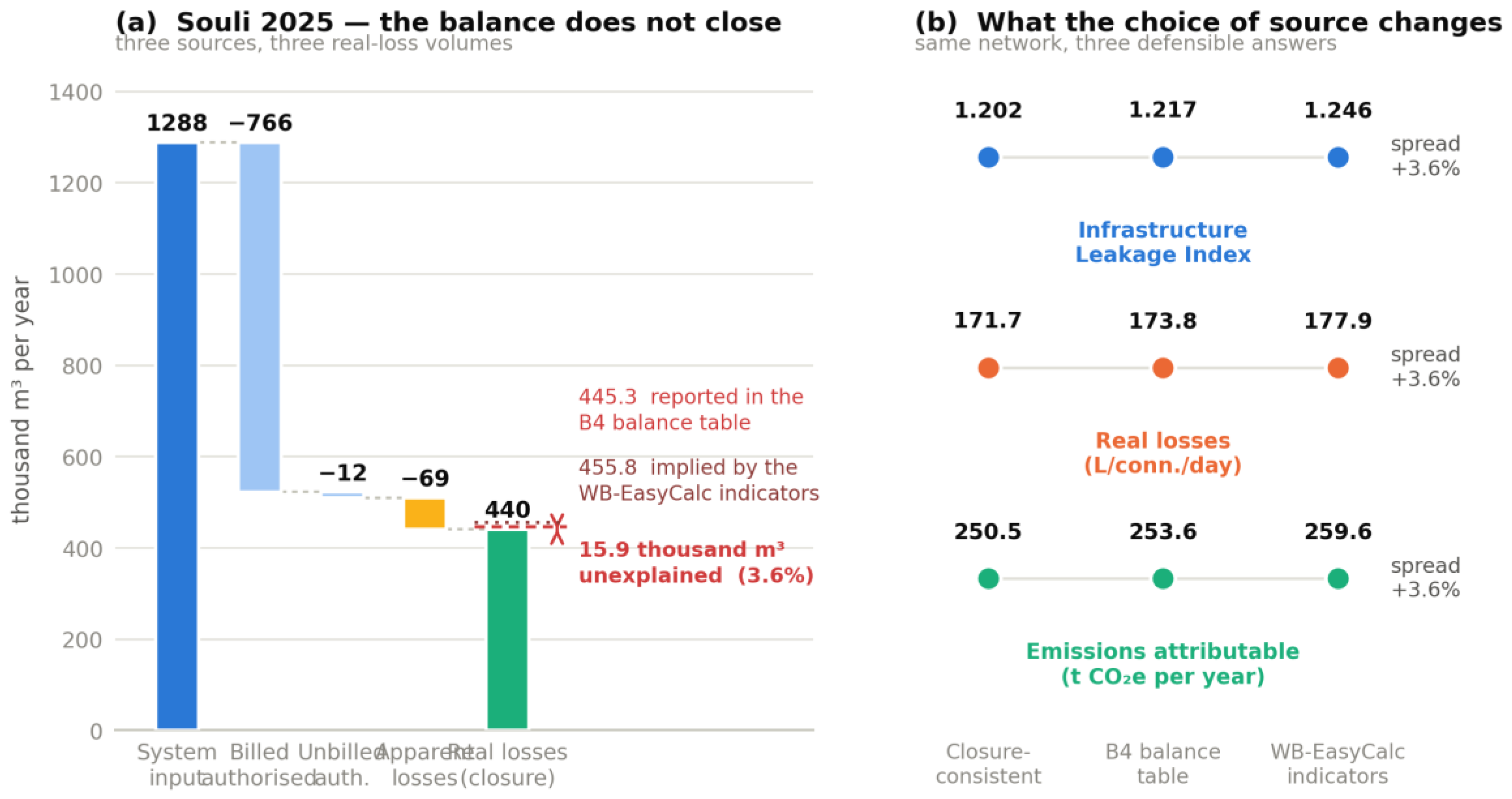
For Souli 2025 the reported system input volume is 1,287,740 m³ and the reported authorised consumption 778,330 m³, which reconciles exactly with its four components. Subtracting authorised consumption and the reported apparent losses of 69,480 m³ leaves 439,930 m³ of real losses. The Β4 balance table reports real losses of 445,320 m³, the sum of its three leakage components. The WB-EasyCalc indicator set reports a current annual real-loss rate of 1,248.9 m³/day, which annualises to 455,849 m³. The three figures span 15,919 m³, or 3.6% of the smallest. Consistent with this, the reported non-revenue water of 527,300 m³ exceeds system input volume minus billed authorised consumption by 5,390 m³.
None of these gaps is large in absolute terms and none affects the qualitative picture of a network losing roughly a third of its supply. They matter because they propagate: the Infrastructure Leakage Index is 1.202, 1.217 or 1.246 depending on which real-loss volume is used; real losses per connection per day are 171.7, 173.8 or 177.9; and the emissions attributable to those losses are 250.5, 253.6 or 259.6 t CO₂e per year. The three figures purport to describe the same physical quantity, so they cannot all be correct; the available provenance does not allow this audit to determine which is. Table 6 therefore reports ranges where the sources disagree.
Three points follow.
First, on terminology: what earlier work has sometimes called embodied carbon in leakage is more accurately described as operational electricity-related emissions attributable to real losses, since it is the energy used to abstract, treat and pump the lost water and not the carbon embodied in construction materials. Similarly, the tariff value of non-revenue water is a gross tariff-equivalent figure, not recoverable revenue: a substantial share of real losses could not be sold even if the network were perfect.
Second, disaggregating energy matters. Attributing Souli’s entire municipal electricity consumption to water gives a carbon intensity of 1.241 kg CO₂e/m³; isolating the water-supply accounts gives 0.569, a factor of 2.2. In our earlier work across a larger sample the corresponding distortion was larger still [18]. Since the recast Drinking Water Directive obliges Member States to assess and report leakage [46] and municipal climate plans increasingly attach carbon values to water losses [19], the allocation step is not optional.
Third, the Infrastructure Leakage Index requires careful handling in this size class, and Figure 10 shows why.
Souli returns an index between 1.20 and 1.25, nominally near-optimal, while losing about 34% of system input as real losses. The reconciliation lies in the allowance. Decomposing the standard formulation shows that 50.6% of Souli’s unavoidable-loss allowance comes from the mains-length term alone, against 14.4% at Aigialeia and 8.1% at Argos–Mycenae. At 14.9 connections per kilometre and 60 m mean operating pressure, Souli is allowed 1,002.4 m³/day of unavoidable loss, which is roughly four fifths of what it actually loses. Lambert’s own review of a decade of application identifies low connection density and atypical pressure as the boundary of the formulation’s validity [55,56]. Reporting an index of 1.25 for Souli without that caveat would be arithmetically correct and substantively misleading. The complementary indicator—real losses per connection per day per metre of pressure—ranks the three utilities identically (9.21, 6.55, 2.86–2.97) without the same sensitivity to the density term, and is the more defensible comparator in this size class. This limitation of the indicator should not be read as a finding about the network.
4. Discussion
4.1. Where the Chain Breaks, and Why It Is Not the Obvious Place
The dominant framing of municipal water digitalisation treats capability as cumulative: add sensors, add connectivity, add a model, and decision support emerges. Our results suggest that capability in a sensor-to-decision pathway is serial rather than cumulative, so the operative question is not how much has been installed but where the chain is thinnest.
Among the technically observable layers, the recurrent thin points are data management, which is chain-limiting in all three cases, and transmission, which is chain-limiting in two of the three. Documentary decision traceability sits at the same level everywhere, subject to the retrieval-scope limitation of Section 3.7. The modelling layer–the part that attracts most research attention—is never the chain-limiting one, and it is the highest-scoring layer at Argos–Mycenae; at Aigialeia it ties with sensing and transmission, and at Souli it sits below sensing. Model capability is therefore not what binds any of these systems, which is a weaker and more accurate statement than saying it is uniformly their strength. Sacoto-Cabrera et al., mapping the IoT–artificial-intelligence–digital-twin literature, identify semantic interoperability and end-to-end data flow as the recurring unresolved problem rather than any individual component technology [57]. Zaman et al. note that the canonical perception–network–application stack is typically evaluated layer by layer, which obscures failures at the interfaces [58]. Syed et al. observe that architectural choices between cloud, fog and edge processing are frequently made at design time and never revisited [59]. What we find in Greek municipal networks is the operational residue of exactly those interface gaps.
The consequence is that completion reporting and functional capability diverge. On conventional indicators—sensors deployed, platform delivered, model built, users trained—all three projects register as successful, and in terms of capital assets delivered they were. Calibration is not among those common indicators: only one of the three evidenced it. Patrão et al.’s critique of assessment tools anticipates this: instruments weighted toward technology presence and evaluated at a single point in time cannot distinguish a functioning system from a commissioned one [25]. Gazzeh’s finding that the technology dimension ranks last when smart-city indicators are prioritised by content analysis points the same way [60].
Two properties make transmission and data management fail quietly. Sensors and platforms are capital items with delivery dates and acceptance tests; data continuity is an operating condition that degrades without producing an artefact. And a dead channel looks exactly like a channel legitimately reading zero—which, as Section 3.3 shows, is not an analogy but the literal situation in Souli, where the diagnostic tags that would separate the two are specified in the project I/O documentation, are not verified as installed or commissioned, and are absent from the export examined. Velaga et al. note that most edge-artificial-intelligence deployments in smart cities remain experimental precisely because sustained operation is harder than initial function [61]. Sobral et al. are instructive by contrast, demonstrating a serverless storage and alerting backend for municipal IoT operated at low annual cost [62], and Belli et al.’s multi-service deployment in Parma shows the organisational counterpart: shared municipal networking infrastructure operated as a utility in its own right, rather than as a set of per-project silos [63].
The metadata failure is equally structural. Souli’s unpopulated register leaves 119 instrument tags without a machine-readable statement of measurand or unit, which is the condition the FAIR principles are written against [33] and which He et al.’s ontology framework and Osolinskyi et al.’s semantic ingestion core are designed to prevent [21,64]. Where that commitment is absent, an archive’s interpretability decays with staff turnover—an acute risk in a municipality with one or two technical staff. Section 3.4 shows the cost concretely: without a unit dictionary, pH readings of 3.7 and 9.5 from two instruments in the same network cannot be reconciled, and neither can be used for compliance.
Aigialeia’s schema drift deserves a separate note because it is the failure mode most likely to recur. The expansion from 23 to 63 columns over 2019 is not a defect; it is the correct physical record of stations being progressively commissioned. It becomes a defect only because it was written to a flat file with no schema versioning. This is the scenario for which Badreddine et al. developed their urban digital twin framework for data-scarce environments, treating incomplete and evolving data as the design premise rather than the exception [65].
4.2. Small Utilities Are Not Scaled-Down Cities
The three cases span 7,019 to 42,000 connections, and none behaves like a miniature of a metropolitan utility.
Souli’s connection density of 14.9 per kilometre is the clearest illustration. It places the utility at the edge of the range over which the Infrastructure Leakage Index behaves as intended, as Section 3.9 quantifies, and it inverts the economics of instrumentation: 470 km of mains serving 7,019 connections means that per-connection sensor cost for equivalent spatial coverage is roughly an order of magnitude above Argos–Mycenae’s. Kapanski et al.’s geospatial clustering approach offers a route through this by optimising zone definition before instrumenting rather than after [66], and Riyahi et al. supply the formal machinery for network partitioning [67]. Neither was applied in any of the three cases; pilot zones were selected pragmatically on existing valve boundaries and available supervisory points.
Mashau et al.’s readiness factors for small and rural municipalities anticipate the institutional side [7]; Das et al. converge on a similar cluster of barriers in resource-constrained urban contexts [68]; Mitieka et al.’s structural modelling of adoption barriers distinguishes driving from dependent barriers, and applied here would likely place data-stewardship capacity among the former and decision integration among the latter [69]. Hiller et al. add the governance dimension we observed but did not systematically measure: ownership and operation of an urban digital twin frequently sit with different parties. In the material we examined, the project deliverables and the analytical outputs were produced by the university and consultant partners rather than by utility staff, though we did not establish who operated the platforms day to day [70]. Lafioune et al.’s municipal maturity framework and Esteban-Narro et al.’s stakeholder methodology both bear directly on that arrangement [28,71].
4.3. Implications for Urban Operations and for the Wider Literature
We take the result to bear on urban operations generally, and state the basis for that carefully. Nothing in the audit is evidence about mobility, waste or building-energy systems; what transfers is the diagnostic, not the finding. What the three cases establish is that a five-layer sensor-to-decision chain can be scored from retrievable artefacts alone, without access to the operator’s premises or to the vendor’s system, and that scoring it locates the binding constraint at a named layer. Any municipal service built on the same stack—instrumentation, telemetry, an archive, an analytical model, an operational procedure—can be examined the same way, and a city running several of them can place them on one scale rather than on the separate vocabularies of their vendors.
Two features of what we found are properties of the municipality rather than of water. The first is that failure concentrated in the layers that have no delivery date. Sensors, platforms and models are capital items with acceptance tests; channel liveness, schema stability and tag metadata are operating conditions that degrade without producing an artefact, and they degrade under the same staffing and the same maintenance budget whatever the instrument is measuring. The second is that an authority with one or two technical staff cannot sustain a separate data-stewardship practice per service. Belli et al.’s multi-service deployment in Parma is the constructive version of the same observation: municipal networking and data infrastructure operated once, as a utility in its own right, rather than rebuilt inside each project [63]. Where instead every funded project delivers its own vertical, as in all three cases here, the stewardship gap is reproduced service by service.
Three consequences follow for a city authority rather than for a water utility. Acceptance of any instrumented urban system can be conditioned on a demonstrated observation window rather than on installed capability, and that criterion is written the same way for a traffic counter as for a pressure logger. A tag-level metadata register—measurand, unit, expected range, diagnostic status—can be held as a cross-service municipal asset rather than as a per-project deliverable, since it is the artefact whose absence left half the Souli channels uninterpretable and the one most readily shared between domains. And the layer at which a city’s digital-twin ambition should be judged is the thinnest one, not the most visible: on our evidence the visible layers—sensors in the ground, a platform with a map—were not where the chain failed. For small and medium-sized cities, which Esteban-Narro et al. [9] and Correia et al. [10] show to be systematically under-represented in the smart-city record, that reordering is the practical content of the result.
For the literature, three further implications follow.
The digital twin taxonomy needs an operational rather than an architectural criterion. Mousavi et al. distinguish model, shadow and twin by the direction and automation of data flow [20]. Applied here, Argos qualifies as a twin by architecture and as a model by operation, because the flow it is designed to carry is not flowing. We suggest that maturity claims be evidenced by an observation-window statistic over a stated period rather than by architectural description.
The leak-detection literature’s reliance on synthetic data is a more serious limitation than it is usually presented as being. Zuñiga-Uribe et al. document that reliance across 53 studies [3]; Mashhadi et al.’s six-algorithm comparison, though conducted on a real campus network, still presumes a continuous labelled input stream [72]. Our audit indicates that the field data required to validate such methods in small utilities does not currently exist in retrievable form, even where the instrumentation to produce it has been deployed. Joseph et al.’s comparison of threshold-based and machine-learning approaches on real supervisory data is valuable precisely because it addresses that regime [73], as are Carrição et al.’s tools for Portuguese utilities of comparable scale [74], Fan et al.’s deployability-oriented detection strategy [75] and Serafeim et al.’s review of estimation methods and mitigation strategies [76]. Mounce et al.’s novelty-detection work illustrates what continuous data would make possible [77].
The water–energy link is being severed at the measurement layer. Ramos et al. position the smart water grid as the mechanism through which water and energy efficiency are jointly optimised [78]; Nagapurkar et al. quantify energy savings from leak reduction [79]; Issa Zadeh and Garay-Rondero place water inside the urban carbon frame [80]; Esfandi et al. document the urban energy planning gap [81]. Colombo and Karney established two decades ago that leakage carries an energy cost distinct from its volumetric cost [82]. All of this requires pump-energy time series. In Souli the active-power channel is among the most frequently non-varying in the export, and the eleven of seventeen station power columns that do carry values do so only at monthly resolution. The link survives in the annual inventory, where Souli’s real losses convert to 250–260 t CO₂e, but it is unavailable at the timescale at which it could be managed.
4.4. Governance and Funding: What We Can and Cannot Conclude
It is tempting to conclude from these results that funding instruments reward procurement over operation. We did not analyse the contracts, acceptance criteria or budget allocations of the three projects, and we therefore state that proposition as a hypothesis consistent with our observations rather than as a finding. What we can say is narrower: the deliverables we examined document design, installation and training, and we found no deliverable requiring evidence of sustained data production, channel liveness or decision uptake. Whether such requirements existed elsewhere in the contractual chain is outside our evidence.
On that basis we offer the following as a testable proposal rather than a demonstrated remedy. An acceptance criterion expressed as a demonstrated observation window—a defined number of consecutive days at the specified sampling interval, with stated thresholds for channel liveness and temporal completeness—would make the failure mode we document visible at the point where it could still be corrected. Purely to make the proposal concrete, and not as a recommended standard: ninety consecutive days at the contracted sampling interval, with at least 95% of contracted channels returning at least one value distinct from their initialisation state and at least 95% temporal completeness against the contracted interval. We attach no evidential weight to these particular numbers. Establishing defensible thresholds would require published evidence on achievable telemetry availability in municipal water networks, which to our knowledge does not exist; producing it would be a useful contribution in itself. ISO 8000-61 provides the process-capability vocabulary for such a requirement [31] and ISO 55000 the asset-management framing for the reactive-to-condition-based transition it would enable [83].
Two further considerations bear on any such design. Prioritisation among competing water interventions is itself a structured decision problem, and Bouramdane’s multi-criteria treatment offers a defensible method for a municipality that cannot fund everything [84]. And continuous telemetry on infrastructure introduces exposure that none of the three projects systematically addressed; Ahmadi-Assalemi et al. set out the minimum expectations for cyber-physical municipal systems [85].
The regulatory context makes this timely. The recast Drinking Water Directive requires risk-based monitoring from catchment to tap and obliges Member States to assess and report leakage [46]; the Water Framework Directive’s cost-recovery provisions require the economic valuation that Souli’s audit supplies [86]; ISO 24512 frames utility management in terms that presume a functioning indicator base [87]. Greece’s managerial-competence regime has since 2023 obliged utilities to submit harmonised water balances, loss indicators, carbon inventories and cost-recovery statements, which is why Table 6 exists at all. That regime is producing annual indicators across the sector—albeit, as Section 3.9 shows, indicators whose own source artefacts disagree. The telemetry investment is producing usable monthly data in one of our three cases and usable daily data outside the reference window in another.
4.5. Limitations
Five limitations bound these conclusions.
The sample is three purposively selected cases in one country under one funding instrument. The shared template makes the comparison informative; it also means the results speak to this delivery model and generalise elsewhere only by argument. Kaluarachchi’s preconditions for data-driven municipal applications may weigh differently in other administrative traditions [88].
The S2D-CMM is an ordinal instrument. The rubric in Table 3 makes it checkable but not validated; equal treatment of the five layers is a choice; and pre-reconciliation agreement rests on fifteen items, too few for a stable kappa estimate. An independent re-scoring is required before the instrument should be used elsewhere.
Two of the four authors were involved in the deployments assessed. The rubric and evidence table are published so that scores can be contested, and the sensitivity analysis shows the principal conclusion does not depend on the contested items; but confirmation bias cannot be excluded by these means alone.
The response window for retrieval requests was short. Requests were issued and the audit cut-off followed within the same reporting cycle, which is not a reasonable interval in which to expect a database export from a municipal technical service. The Argos transmission and data-management scores rest on non-supply within that window and should be read accordingly; Section 3.8 reports the consequence of assuming the archive exists and is complete, which is that the chain-limited level does not move.
The retrieval scope bounds the decision-layer finding. Six classes of artefact in which a telemetry-driven decision would most plausibly be recorded—work orders, alarm logs with operator acknowledgements, maintenance tickets, operational meeting minutes, valve and pump setting logs, and operator interviews—were not requested. The L5 scores should be read as statements about documentary discoverability, not about operating practice.
The harmonised reference window was selected after the archives had been examined, not before. Section 3.8 reports the scores under four alternative windows and the conclusions are unchanged, but a prospectively registered window would have been stronger and is what a replication should use.
The audit assesses retrievable archives at one point in time. Data may exist in vendor systems, on devices or in backups not accessible to us; the Argos archive in particular may exist and simply not have been produced. We have scored what an analyst could actually obtain, which we take to be the operationally meaningful test, but that is not proof of absence.
Finally, the three utilities’ submissions are of unequal completeness. Table 6’s dashes are gaps in the source data, not zeros, and the cross-case comparison rests on the subset all three populated. The water-quality findings in Section 3.4 rest on eight field-logger readings and are provisional.
5. Conclusions
We audited three publicly funded IoT deployments in small and medium-sized Greek water utilities to establish whether they close the chain from sensor reading to operational decision. Against an explicit rubric and a harmonised twelve-month window, no such chain could be demonstrated from the evidence retrieved.
Modelling was never the chain-limiting layer in any case, and only one of the three had a documented calibration; model capability is not what binds these systems. Among the technically observable layers the recurrent bottlenecks were data management, chain-limiting in all three cases, and transmission, chain-limiting in two of the three. Documentary decision traceability was at level 1 in all three, although that finding is bounded by the retrieval scope. The retrievable Souli archive holds 240 multivariate one-minute records; 53 of 119 channels do not vary, and the diagnostic tags that would establish whether this reflects instrument failure or idle plant are specified in the project I/O documentation, are not verified as installed or commissioned, and are absent from the export examined. Aigialeia’s daily series reaches 96.9% within-span completeness but only 48 hours of it are sub-hourly, and its predecessor supervisory system wrote a schema that changed shape within a single reporting year. The Argos archive was not supplied before the audit cut-off. In none of the three cases was a decision traceable to a sensor reading identified in the artefact set retrieved—a narrower claim than the absence of such decisions, since work orders, alarm logs, maintenance tickets, setting logs and operator interviews were outside the retrieval scope and are the first target for follow-up work. The chain-limited level is 1 in all three cases, and remains so under four alternative reference windows.
The utilities are nonetheless not data-poor. Souli’s 2025 audit reports 40.5–40.9% non-revenue water, 34.2–35.4% real losses, a supply energy intensity of 1.55 kWh/m³ and 250–260 t CO₂e attributable to its real losses. That capability came from regulatory obligation rather than from instrumentation. Recomputation also showed the statutory reporting artefacts disagreeing by 3.6% on real losses, which moves the reported Infrastructure Leakage Index from 1.20 to 1.25 and illustrates that indicator harmonisation is unfinished even where reporting is mandatory.
Lifting any of these systems requires more than one change: Aigialeia is two layer-improvements from a chain-limited level of 2, the other two are three. Four propositions follow, offered as hypotheses for testing rather than as demonstrated remedies. Acceptance of telemetry projects could be conditioned on a demonstrated observation window rather than on installed capability. A populated metadata register giving measurand and unit for every tag could be made a deliverable in its own right; without it, values arrive uninterpretable, as Section 3.4 shows for pH. Diagnostic and status signals could be required in the data export and not only in the control-system specification, since without them a zero cannot be interpreted. And functional disaggregation of municipal electricity accounts could be required, since without it the carbon intensity of supplied water is wrong by a factor of two in the case examined here.
Two directions for further work follow. Empirically, applying the rubric to a larger and more heterogeneous sample, with independent raters, would establish whether the concentration of failure in the data-chain layers—data management in all three cases here, transmission in two of the three—is general, and whether documentary decision traceability sits at level 1 as widely as it does here once the retrieval scope is widened to the artefact classes listed in Table S2c and would allow the treatment of layers to be estimated rather than assumed. Technically, where stewardship capacity is the binding constraint, agent-based approaches that automate ingestion, validation and anomaly reporting—of the kind Choi and Yoon propose for intelligent urban digital twins [89]—may suit a municipality with two technical staff better than additional instrumentation, and open-source implementations of the type demonstrated by Lopez-Cabeza et al. reduce the dependence on a single vendor that makes continuity fragile [90]. Greek experience with multi-pilot environmental data platforms offers a domestic precedent for both [91].
The wider implication is that the problem in small-municipality smart water systems is not primarily a technology gap. The technology was procured and documented as delivered and, in the modelling layer, competently configured. What was not established is the practice of keeping data flowing, interpretable and acted upon. That practice is not held by a water department; it is held, or not held, by the municipality. For a city operating several instrumented services on one technical staff and one procurement regime, the layer-by-layer test used here transfers even though the findings do not, and it identifies where a smart-city programme is most likely to be open-loop before further instrumentation is bought.
Supplementary Materials
The supplementary information can be downloaded at the website of this paper posted on Preprints.org. The following are available online. Table S1, per-item evidence behind each of the fifteen S2D-CMM scores, with a column reserved for the blind pass described in Section 2.6. Table S2, the retrieval log: every artefact examined, its source path, size, retrieval date and outcome, including the requests not supplied by the audit cut-off and the artefact classes that were not requested. Table S3, the Souli 2025 water-balance reconciliation, the unavoidable-loss decomposition and the sensitivity of the downstream indicators to the choice of real-loss basis. Table S4, the channel classification for the Souli one-minute export. Table S5, the Souli water-quality readings from both sources. Table S6, the gap structure of the Aigialeia daily series. Table S7, the reference-window sensitivity computation. Table S8, the blind re-scoring protocol. Table S9, a summary of the three robustness checks and of the one that was withdrawn. Dataset S1 (derived_indicators.csv), the derived indicator dataset and the scoring matrix. Code S1 (code_s1.zip), ten files: the balance-reconciliation, window-sensitivity, blind-score ingestion, figure-generation and package-verification scripts, the blind-score template, a shared plotting-constants module, a README giving the environment, inputs, run order and outputs, and the manuscript and supplement in markdown source form, which the verification harness reads.
Author Contributions
Conceptualization, A.C. and P.T.N.; methodology, A.C. and D.P.; software, A.C.; validation, T.N. and P.T.N.; formal analysis, A.C.; investigation, A.C.; data curation, A.C.; writing—original draft preparation, A.C.; writing—review and editing, T.N., D.P. and P.T.N.; visualization, A.C.; supervision, P.T.N. and D.P. All authors have read and agreed to the published version of the manuscript.
Funding
This secondary analysis received no external funding. The three deployments examined were financed by the EEA Financial Mechanism 2014–2021, Programme “Water Management”. The individual project reference numbers were not present in any artefact examined during the audit and are therefore not reported here. The programme operator had no role in the design, analysis, interpretation, writing or publication decision for the present study.
Institutional Review Board Statement
Not applicable.
Data Availability Statement
The derived indicator dataset (Dataset S1), the scoring matrix and the processing code (Code S1) are provided as Supplementary Material and contain no confidential material. The primary telemetry archives, project deliverables and regulatory submissions are the property of the Municipality of Souli, DEYA Argos–Mycenae and DEYA Aigialeia respectively and are available from them subject to authorisation; Table S2 gives the source path of every artefact examined so that a request can be made for any of them specifically. The three utilities consented to being identified by name in this publication.
Acknowledgments
The authors thank the technical services of the Municipality of Souli, DEYA Argos–Mycenae and DEYA Aigialeia for access to project documentation and operational records. During the preparation and revision of this manuscript, the authors used AI tools to support English-language editing, stylistic refinement, structural organization, consistency checks across the text, tables, and figures, and the preparation of selected visualizations and Supplementary Tables. The tools were not used to generate primary data, to assign any S2D-CMM score, to determine the study results, or to make final methodological or interpretive decisions. All AI-assisted output was critically reviewed, verified against the underlying data and cited sources, and revised by the authors, who take full responsibility for the accuracy, integrity, and final content of the manuscript.
Conflicts of Interest
This study assesses projects in which some of the authors participated, and the disclosure is therefore given in detail. A.C. is affiliated with WEST Consulting Engineers, which provided technical services in connection with the SMASH (Souli) and SWAN (Aigialeia) projects, and is a co-author of prior publications reporting on both. D.P. is affiliated with the University of West Attica, the academic partner in the SWAN project, and is a co-author of the prior publication reporting on it. P.T.N. is a co-author of prior publications reporting on both projects. T.N. had no role in any of the three deployments assessed. The S2D-CMM scoring described in Section 2.6 was performed by A.C. and D.P., both of whom had project involvement. We regard this as a material limitation rather than a disclosed formality. Three mitigations were applied: the scoring rubric is published in full (Table 3) so that any score can be contested against a stated criterion; the evidence behind each of the fifteen scores is published (Table S1); and three robustness checks (Section 3.8) report what would have to change for the conclusion to move, how it behaves when the two contested scores are varied across the range the scorers proposed, and how it behaves under four alternative reference windows. An earlier version reported a fourth exercise that held the decision layer fixed while varying the data layers; that exercise is withdrawn in Section 3.8 as uninformative, since it could only restate the definition of a minimum. Where the two scorers disagreed, the lower score was adopted, which is the direction unfavourable to the projects with which the scorers were associated. A blind re-scoring protocol for the author with no project involvement is specified in Table S8 and has not yet been executed; Section 2.6 records this. No re-scoring by a rater external to the author team has been performed either. We identify independent scoring as the first requirement for any application of the instrument beyond these three cases, and the scores reported here should be read as the reconciled judgement of two raters with project involvement.
Abbreviations
| CARL | Current Annual Real Losses |
| DEYA | Municipal Enterprise for Water Supply and Sewerage (Greece) |
| DMA | District Metered Area |
| DWD | Drinking Water Directive |
| GIS | Geographic Information System |
| ILI | Infrastructure Leakage Index |
| IoT | Internet of Things |
| IWA | International Water Association |
| I/O | Input/Output |
| NRW | Non-Revenue Water |
| S2D-CMM | Sensor-to-Decision Capability Maturity Model |
| SCADA | Supervisory Control and Data Acquisition |
| UARL | Unavoidable Annual Real Losses |
References
- Grigg, N.S. Digital Transformation in Water Utilities: Status, Challenges, and Prospects. Smart Cities 2025, 8, 99. [Google Scholar] [CrossRef]
- Azadi, S.; Kasraian, D.; Nourian, P.; van Wesemael, P. What Have Urban Digital Twins Contributed to Urban Planning and Decision Making? From a Systematic Literature Review Toward a Socio-Technical Research and Development Agenda. Smart Cities 2025, 8, 32. [Google Scholar] [CrossRef]
- Zuñiga-Uribe, M.; Rojas-Galván, R.; Álvarez-Alvarado, J.M.; Aviles, M.; Pérez-Soto, G.I.; Pérez-Moreno, V. Artificial Intelligence in Water Distribution Networks: A Systematic Review of Models, Input Variables, Databases, and Output Strategies for Leak Detection. Smart Cities 2026, 9, 45. [Google Scholar] [CrossRef]
- Rajan, G.; Li, S. A Systematic Literature Review on Flow Data-Based Techniques for Automated Leak Management in Water Distribution Systems. Smart Cities 2025, 8, 78. [Google Scholar] [CrossRef]
- Ghorbani Bam, P.; Rezaei, N.; Roubanis, A.; Austin, D.; Austin, E.; Tarroja, B.; Takacs, I.; Villez, K.; Rosso, D. Digital Twin Applications in the Water Sector: A Review. Water 2025, 17, 2957. [Google Scholar] [CrossRef]
- Berg, S.; Marques, R. Quantitative Studies of Water and Sanitation Utilities: A Benchmarking Literature Survey. Water Policy 2011, 13, 591–606. [Google Scholar] [CrossRef]
- Mashau, N.L.; Kroeze, J.H.; Howard, G.R. Key Factors for Assessing Small and Rural Municipalities’ Readiness for Smart City Implementation. Smart Cities 2022, 5, 1742–1751. [Google Scholar] [CrossRef]
- Grigg, N. Economic Framework of Smart and Integrated Urban Water Systems. Smart Cities 2022, 5, 241–250. [Google Scholar] [CrossRef]
- Esteban-Narro, R.; Lo-Iacono-Ferreira, V.G.; Torregrosa-López, J.I. Evaluating Smart and Sustainable City Projects: An Integrated Framework of Impact and Performance Indicators. Smart Cities 2025, 8, 172. [Google Scholar] [CrossRef]
- Correia, D.; Marques, J.L.; Teixeira, L. The State-of-the-Art of Smart Cities in the European Union. Smart Cities 2022, 5, 1776–1810. [Google Scholar] [CrossRef]
- Bell, E.V.; Hansen, K.; Mullin, M. Assessing Performance and Capacity of US Drinking Water Systems. J. Water Resour. Plan. Manag. 2023, 149, 05022011. [Google Scholar] [CrossRef]
- EEA Grants Greece. Programme “Water Management” (EEA Financial Mechanism 2014–2021); Ministry of Environment and Energy: Athens, Greece; Available online: https://www.eeagrants.gr/programmes/programme-d/?lang=en (accessed on 21 August 2026).
- Yin, R.K. Case Study Research and Applications: Design and Methods, 6th ed.; SAGE Publications: Thousand Oaks, CA, USA, 2018; ISBN 978-1-5063-3616-9. [Google Scholar]
- Eisenhardt, K.M. Building Theories from Case Study Research. Acad. Manag. Rev. 1989, 14, 532–550. [Google Scholar] [CrossRef]
- Chasiotis, A.; Piromalis, D.; Papageorgas, P.; Chasiotis, S.; Bousdeki, M.; Nastos, P.T.; Feloni, E. A Smart Integrated Platform for Leakage Detection in the Water Supply Network of Aigio, Greece. Environ. Sci. Proc. 2023, 26, 184. [Google Scholar] [CrossRef]
- Chasiotis, A.; Tsitsifli, S.; Panytsidis, K.; Nilsen, V.; Mantas, N.; Theodorou, D.; Kyriakidis, T.; Chasiotis, S.; Bousdeki, M.; Feloni, E.; Ratnaweera, H.; Nastos, P.; Louta, M. Building a Smart Green System to Control Water Leakage and Monitor Drinking Water Quality in the Water Supply System of Paramythia City, Greece: The Case of SMASH Project. EGU General Assembly 2023, Vienna, Austria, 23–28 April 2023; p. EGU23-10057. [Google Scholar] [CrossRef]
- Chasiotis, A.; Kosiori, M.; Feloni, E.; Gialama, S.; Mathiou, P.; Nastos, P.T. Efficient Leakage Monitoring through Remote Sensing of Water Parameters in Water Distribution Network of Nestos Area, Greece. In Proceedings of SPIE 13816, Eleventh International Conference on Remote Sensing and Geoinformation of the Environment (RSCy2025); SPIE: Bellingham, WA, USA, 2025; p. 138160E. [Google Scholar] [CrossRef]
- Chasiotis, A.; Mathiou, P.; Bousdeki, M.; Pappa, A.; Manthos, T.; Nastos, P.T. Municipal Carbon Footprint and Water Infrastructure: A Comparative Assessment of Emission Reduction Plans in Three Greek Municipalities. Water 2026, 18, 1020. [Google Scholar] [CrossRef]
- Chasiotis, A.; Mathiou, P.; Pappa, A.; Nikolaou, T.; Bousdeki, M.; Manthos, T.; Nastos, P.T. Comparative Analysis of Local Climate Neutrality Action Plans: The Municipal Emission Reduction Plans of Spetses, Platanias and Souli as Pathways to Climate Neutrality and Territorial Restructuring. Sustain. Dev. Cult. Tradit. J. (In Greek) 2026, 2026/1, 65–87. [Google Scholar]
- Mousavi, Y.; Gharineiat, Z.; Karimi, A.A.; McDougall, K.; Rossi, A.; Gonizzi Barsanti, S. Digital Twin Technology in Built Environment: A Review of Applications, Capabilities and Challenges. Smart Cities 2024, 7, 2594–2615. [Google Scholar] [CrossRef]
- Osolinskyi, O.; Lipianina-Honcharenko, K.; Komar, M. Semantic Core for Sensor Telemetry Ingestion for Digital Twins. Smart Cities 2026, 9, 77. [Google Scholar] [CrossRef]
- Ntafalias, A.; Tsakanikas, S.; Skarvelis-Kazakos, S.; Papadopoulos, P.; Skarmeta-Gómez, A.F.; González-Vidal, A.; Tomat, V.; Ramallo-González, A.P.; Marin-Perez, R.; Vlachou, M.C. Design and Implementation of an Interoperable Architecture for Integrating Building Legacy Systems into Scalable Energy Management Systems. Smart Cities 2022, 5, 1421–1440. [Google Scholar] [CrossRef]
- Villar Miguelez, C.; Monzon Baeza, V.; Parada, R.; Monzo, C. Guidelines for Renewal and Securitization of a Critical Infrastructure Based on IoT Networks. Smart Cities 2023, 6, 728–743. [Google Scholar] [CrossRef]
- Ciliberti, F.G.; Berardi, L.; Laucelli, D.B.; Ariza, A.D.; Enriquez, L.V.; Giustolisi, O. From Digital Twin Paradigm to Digital Water Services. J. Hydroinform. 2023, 25, 2444–2459. [Google Scholar] [CrossRef]
- Patrão, C.; Moura, P.; de Almeida, A.T. Review of Smart City Assessment Tools. Smart Cities 2020, 3, 1117–1132. [Google Scholar] [CrossRef]
- Aljowder, T.; Ali, M.; Kurnia, S. Development of a Maturity Model for Assessing Smart Cities: A Focus Area Maturity Model. Smart Cities 2023, 6, 2150–2175. [Google Scholar] [CrossRef]
- Angelakoglou, K.; Nikolopoulos, N.; Giourka, P.; Svensson, I.-L.; Tsarchopoulos, P.; Tryferidis, A.; Tzovaras, D. A Methodological Framework for the Selection of Key Performance Indicators to Assess Smart City Solutions. Smart Cities 2019, 2, 269–306. [Google Scholar] [CrossRef]
- Lafioune, N.; Poirier, E.A.; St-Jacques, M. Managing Urban Infrastructure Assets in the Digital Era: Challenges of Municipal Digital Transformation. Digit. Transform. Soc. 2024, 3, 3–22. [Google Scholar] [CrossRef]
- Lawrence, N.D. Data Readiness Levels. arXiv 2017, arXiv:1705.02245. [Google Scholar] [CrossRef]
- ISO/IEC 25012:2008; Software Engineering—Software Product Quality Requirements and Evaluation (SQuaRE)—Data Quality Model. International Organization for Standardization: Geneva, Switzerland, 2008.
- ISO 8000-61:2016; Data Quality—Part 61: Data Quality Management: Process Reference Model. International Organization for Standardization: Geneva, Switzerland, 2016.
- DAMA International. DAMA-DMBOK: Data Management Body of Knowledge, 2nd ed.; Technics Publications: Bradley Beach, NJ, USA, 2017; ISBN 978-1-63462-234-9. [Google Scholar]
- Wilkinson, M.D.; Dumontier, M.; Aalbersberg, I.J.; Appleton, G.; Axton, M.; Baak, A.; Blomberg, N.; Boiten, J.-W.; da Silva Santos, L.B.; Bourne, P.E.; et al. The FAIR Guiding Principles for Scientific Data Management and Stewardship. Sci. Data 2016, 3, 160018. [Google Scholar] [CrossRef]
- Lambert, A.; Hirner, W. Losses from Water Supply Systems: Standard Terminology and Recommended Performance Measures; IWA Blue Pages; International Water Association: London, UK, 2000. [Google Scholar]
- Alegre, H.; Baptista, J.M.; Cabrera, E., Jr.; Cubillo, F.; Duarte, P.; Hirner, W.; Merkel, W.; Parena, R. Performance Indicators for Water Supply Services, 3rd ed.; IWA Publishing: London, UK, 2016; ISBN 978-1-78040-632-9. [Google Scholar]
- American Water Works Association. M36 Water Audits and Loss Control Programs, 5th ed.; AWWA: Denver, CO, USA, 2024; ISBN 978-1-64717-154-4. [Google Scholar]
- ISO 14064-1:2018Greenhouse Gases—Part 1: Specification with Guidance at the Organization Level for Quantification and Reporting of Greenhouse Gas Emissions and Removals, 2nd ed.; International Organization for Standardization: Geneva, Switzerland, 2018.
- Gamboa-Medina, M.M.; Reis, L.F.R. Sampling Design for Leak Detection in Water Distribution Networks. Procedia Eng. 2017, 186, 460–469. [Google Scholar] [CrossRef]
- Piazza, S.; Sambito, M.; Freni, G. Analysis of Optimal Sensor Placement in Looped Water Distribution Networks Using Different Water Quality Models. Water 2023, 15, 559. [Google Scholar] [CrossRef]
- Serafeim, A.V.; Kokosalakis, G.; Deidda, R.; Karathanasi, I.; Langousis, A. Probabilistic Minimum Night Flow Estimation in Water Distribution Networks and Comparison with the Water Balance Approach: Large-Scale Application to the City Center of Patras in Western Greece. Water 2022, 14, 98. [Google Scholar] [CrossRef]
- Tricarico, C.; Cappello, C.; de Marinis, G.; Leopardi, A. Minimum Night Flow Estimation in District Metered Areas. Water 2024, 16, 3642. [Google Scholar] [CrossRef]
- Alassio, S.; Marsili, V.; Mazzoni, F.; Alvisi, S. Exploring Residential Minimum Night Consumption in a Real Water Distribution Network Based on Smart-Meter Data. Discov. Water 2024, 4, 88. [Google Scholar] [CrossRef]
- Branisavljević, N.; Kapelan, Z.; Prodanović, D. Improved Real-Time Data Anomaly Detection Using Context Classification. J. Hydroinform. 2011, 13, 307–323. [Google Scholar] [CrossRef]
- Quevedo, J.; Puig, V.; Cembrano, G.; Blanch, J.; Aguilar, J.; Saporta, D.; Benito, G.; Hedo, M.; Molina, A. Validation and Reconstruction of Flow Meter Data in the Barcelona Water Distribution Network. Control Eng. Pract. 2010, 18, 640–651. [Google Scholar] [CrossRef]
- Osman, M.S.; Abu-Mahfouz, A.M.; Page, P.R. A Survey on Data Imputation Techniques: Water Distribution System as a Use Case. IEEE Access 2018, 6, 63279–63291. [Google Scholar] [CrossRef]
- Directive (EU) 2020/2184 of the European Parliament and of the Council of 16 December 2020 on the Quality of Water Intended for Human Consumption (Recast). Off. J. Eur. Union 2020, L 435, 1.
- Herold, G.; Rodino, F.; Prévoteau, A.; Carrara, S.; Reynaert, E. Long-Term Performance of Low-Cost Free Chlorine Sensors to Monitor On-Site Water Reuse. Water Sci. Technol. 2025, 92, 326–339. [Google Scholar] [CrossRef]
- Aisopou, A.; Stoianov, I. Evaluation of Free-Chlorine Data from Online Sensors in a Water Supply Network. Eng. Proc. 2024, 69, 144. [Google Scholar] [CrossRef]
- World Health Organization. Water Safety Plan Manual: Step-by-Step Risk Management for Drinking-Water Suppliers, 2nd ed.; WHO: Geneva, Switzerland, 2023; ISBN 978-92-4-006769-1. [Google Scholar]
- Tsitsifli, S.; Tsoukalas, D.S. Water Safety Plans and HACCP Implementation in Water Utilities around the World: Benefits, Drawbacks and Critical Success Factors. Environ. Sci. Pollut. Res. 2021, 28, 18837–18849. [Google Scholar] [CrossRef]
- Bonilla, C.A.; Zanfei, A.; Brentan, B.; Montalvo, I.; Izquierdo, J. A Digital Twin of a Water Distribution System by Using Graph Convolutional Networks for Pump Speed-Based State Estimation. Water 2022, 14, 514. [Google Scholar] [CrossRef]
- Adedeji, K.B.; Hamam, Y.; Abe, B.T.; Abu-Mahfouz, A.M. Leakage Detection and Estimation Algorithm for Loss Reduction in Water Piping Networks. Water 2017, 9, 773. [Google Scholar] [CrossRef]
- Sophocleous, S.; Savić, D.; Kapelan, Z. Leak Localization in a Real Water Distribution Network Based on Search-Space Reduction. J. Water Resour. Plan. Manag. 2019, 145, 04019024. [Google Scholar] [CrossRef]
- Ruijer, E.; Van Twist, A.; Haaker, T.; Tartarin, T.; Schuurman, N.; Melenhorst, M.; Meijer, A. Smart Governance Toolbox: A Systematic Literature Review. Smart Cities 2023, 6, 878–896. [Google Scholar] [CrossRef]
- Lambert, A.O.; Brown, T.G.; Takizawa, M.; Weimer, D. A Review of Performance Indicators for Real Losses from Water Supply Systems. J. Water Supply Res. Technol.—AQUA 1999, 48, 227–237. [Google Scholar] [CrossRef]
- Lambert, A.O. Ten Years Experience in Using the UARL Formula to Calculate Infrastructure Leakage Index. In Proceedings of the IWA Water Loss 2009 Conference, Cape Town, South Africa, April 2009. [Google Scholar]
- Sacoto-Cabrera, E.J.; Perez-Torres, A.; Tello-Oquendo, L.; Cerrada, M. IoT, AI, and Digital Twins in Smart Cities: A Systematic Review for a Thematic Mapping and Research Agenda. Smart Cities 2025, 8, 175. [Google Scholar] [CrossRef]
- Zaman, M.; Puryear, N.; Abdelwahed, S.; Zohrabi, N. A Review of IoT-Based Smart City Development and Management. Smart Cities 2024, 7, 1462–1501. [Google Scholar] [CrossRef]
- Syed, A.S.; Sierra-Sosa, D.; Kumar, A.; Elmaghraby, A. IoT in Smart Cities: A Survey of Technologies, Practices and Challenges. Smart Cities 2021, 4, 429–475. [Google Scholar] [CrossRef]
- Gazzeh, K. Ranking Sustainable Smart City Indicators Using Combined Content Analysis and Analytic Hierarchy Process Techniques. Smart Cities 2023, 6, 2883–2909. [Google Scholar] [CrossRef]
- Velaga, K.S.; Guo, Y.; Yu, W. Edge AI for Smart Cities: Foundations, Challenges, and Opportunities. Smart Cities 2025, 8, 211. [Google Scholar] [CrossRef]
- Sobral, V.A.L.; Nelson, J.; Asmare, L.; Mahmood, A.; Mitchell, G.; Tenkorang, K.; Todd, C.; Campbell, B.; Goodall, J.L. A Cloud-Based Data Storage and Visualization Tool for Smart City IoT: Flood Warning as an Example Application. Smart Cities 2023, 6, 1416–1434. [Google Scholar] [CrossRef]
- Belli, L.; Cilfone, A.; Davoli, L.; Ferrari, G.; Adorni, P.; Di Nocera, F.; Dall’Olio, A.; Pellegrini, C.; Mordacci, M.; Bertolotti, E. IoT-Enabled Smart Sustainable Cities: Challenges and Approaches. Smart Cities 2020, 3, 1039–1071. [Google Scholar] [CrossRef]
- He, X.; Kuai, X.; Li, X.; Qiu, Z.; He, B.; Guo, R. Smart City Ontology Framework for Urban Data Integration and Application. Smart Cities 2025, 8, 165. [Google Scholar] [CrossRef]
- Badreddine, O.; Radoine, H.; Hajji, R. TwinCity: An Urban Digital Twin Framework for Data-Scarce Environments—A Case Study of Benguerir, Morocco. Smart Cities 2026, 9, 23. [Google Scholar] [CrossRef]
- Kapanski, A.A.; Klyuev, R.V.; Boltrushevich, A.E.; Sorokova, S.N.; Efremenkov, E.A.; Demin, A.Y.; Martyushev, N.V. Geospatial Clustering in Smart City Resource Management: An Initial Step in the Optimisation of Complex Technical Supply Systems. Smart Cities 2025, 8, 14. [Google Scholar] [CrossRef]
- Riyahi, M.M.; Giudicianni, C.; Haghighi, A.; Creaco, E. Coupled Multi-Objective Optimization of Water Distribution Network Design and Partitioning: A Spectral Graph-Theory Approach. Urban Water J. 2024, 21, 745–756. [Google Scholar] [CrossRef]
- Das, D.K.; Aiyetan, A.O.; Mostafa, M.M.H. Advancing Smart Cities in Africa: Barriers, Potentials, and Strategic Pathways for Sustainable Urban Transformation. Smart Cities 2026, 9, 38. [Google Scholar] [CrossRef]
- Mitieka, D.; Luke, R.; Twinomurinzi, H.; Mageto, J. Mapping the Institutional and Socio-Political Barriers to Smart Mobility Adoption: A TISM-MICMAC Approach. Smart Cities 2025, 8, 182. [Google Scholar] [CrossRef]
- Hiller, J.; Mansour, M.; Kremer, N.; Crampen, D.; von Behren, S. Mapping Urban Digital Twins Across Regions: An Exploratory Study of Maturity, Implementation Status, and Authority. Smart Cities 2026, 9, 49. [Google Scholar] [CrossRef]
- Esteban-Narro, R.; Lo-Iacono-Ferreira, V.G.; Torregrosa-López, J.I. Urban Stakeholders for Sustainable and Smart Cities: An Innovative Identification and Management Methodology. Smart Cities 2025, 8, 41. [Google Scholar] [CrossRef]
- Mashhadi, N.; Shahrour, I.; Attoue, N.; El Khattabi, J.; Aljer, A. Use of Machine Learning for Leak Detection and Localization in Water Distribution Systems. Smart Cities 2021, 4, 1293–1315. [Google Scholar] [CrossRef]
- Joseph, K.; Shetty, J.; Sharma, A.K.; van Staden, R.; Wasantha, P.L.P.; Small, S.; Bennett, N. Leak and Burst Detection in Water Distribution Network Using Logic- and Machine Learning-Based Approaches. Water 2024, 16, 1935. [Google Scholar] [CrossRef]
- Carrição, N.; Ferreira, B.; Antunes, A.; Caetano, J.; Covas, D. Computational Tools for Supporting the Operation and Management of Water Distribution Systems towards Digital Transformation. Water 2023, 15, 553. [Google Scholar] [CrossRef]
- Fan, X.; Zhang, X.; Yu, X.B. Machine Learning Model and Strategy for Fast and Accurate Detection of Leaks in Water Supply Network. J. Infrastruct. Preserv. Resil. 2021, 2, 10. [Google Scholar] [CrossRef]
- Serafeim, A.V.; Fourniotis, N.T.; Deidda, R.; Kokosalakis, G.; Langousis, A. Leakages in Water Distribution Networks: Estimation Methods, Influential Factors, and Mitigation Strategies—A Comprehensive Review. Water 2024, 16, 1534. [Google Scholar] [CrossRef]
- Mounce, S.R.; Mounce, R.B.; Boxall, J.B. Novelty Detection for Time Series Data Analysis in Water Distribution Systems Using Support Vector Machines. J. Hydroinform. 2011, 13, 672–686. [Google Scholar] [CrossRef]
- Ramos, H.M.; Kuriqi, A.; Besharat, M.; Creaco, E.; Tasca, E.; Coronado-Hernández, O.E.; Pienika, R.; Iglesias-Rey, P. Smart Water Grids and Digital Twin for the Management of System Efficiency in Water Distribution Networks. Water 2023, 15, 1129. [Google Scholar] [CrossRef]
- Nagapurkar, P.; Sharma, N.; Garcia, S.; Nimbalkar, S. Evaluating Acoustic vs. AI-Based Satellite Leak Detection in Aging US Water Infrastructure: A Cost and Energy Savings Analysis. Smart Cities 2025, 8, 122. [Google Scholar] [CrossRef]
- Issa Zadeh, S.B.; Garay-Rondero, C.L. Enhancing Urban Sustainability: Unravelling Carbon Footprint Reduction in Smart Cities through Modern Supply-Chain Measures. Smart Cities 2023, 6, 3225–3250. [Google Scholar] [CrossRef]
- Esfandi, S.; Tayebi, S.; Byrne, J.; Taminiau, J.; Giyahchi, G.; Alavi, S.A. Smart Cities and Urban Energy Planning: An Advanced Review of Promises and Challenges. Smart Cities 2024, 7, 414–444. [Google Scholar] [CrossRef]
- Colombo, A.F.; Karney, B.W. Energy and Costs of Leaky Pipes: Toward Comprehensive Picture. J. Water Resour. Plan. Manag. 2002, 128, 441–450. [Google Scholar] [CrossRef]
- ISO 55000:2024Asset Management—Vocabulary, Overview and Principles, 2nd ed.; International Organization for Standardization: Geneva, Switzerland, 2024.
- Bouramdane, A.-A. Optimal Water Management Strategies: Paving the Way for Sustainability in Smart Cities. Smart Cities 2023, 6, 2849–2882. [Google Scholar] [CrossRef]
- Ahmadi-Assalemi, G.; Al-Khateeb, H.; Epiphaniou, G.; Maple, C. Cyber Resilience and Incident Response in Smart Cities: A Systematic Literature Review. Smart Cities 2020, 3, 894–927. [Google Scholar] [CrossRef]
- Directive 2000/60/EC of the European Parliament and of the Council of 23 October 2000 Establishing a Framework for Community Action in the Field of Water Policy. Off. J. Eur. Communities 2000, L 327, 1.
- ISO 24512:2024Activities Relating to Drinking Water and Wastewater Services—Guidelines for the Management of Drinking Water Utilities and for the Assessment of Drinking Water Services, 2nd ed.; International Organization for Standardization: Geneva, Switzerland, 2024.
- Kaluarachchi, Y. Implementing Data-Driven Smart City Applications for Future Cities. Smart Cities 2022, 5, 455–474. [Google Scholar] [CrossRef]
- Choi, S.; Yoon, S. AI Agent-Based Intelligent Urban Digital Twin (I-UDT): Concept, Methodology, and Case Studies. Smart Cities 2025, 8, 28. [Google Scholar] [CrossRef]
- Lopez-Cabeza, V.P.; Videras-Rodriguez, M.; Gomez-Melgar, S. An Open-Source Urban Digital Twin for Enhancing Outdoor Thermal Comfort in the City of Huelva (Spain). Smart Cities 2025, 8, 160. [Google Scholar] [CrossRef]
- Kolokotsa, D.; Lilli, A.; Tsekeri, E.; Gobakis, K.; Katsiokalis, M.; Mania, A.; Baldacchino, N.; Polychronaki, S.; Buckley, N.; Micallef, D.; Calleja, K.; Clarke, E.; Duca, E.; Mali, L.; Bisello, A. The Intersection of the Green and the Smart City: A Data Platform for Health and Well-Being through Nature-Based Solutions. Smart Cities 2024, 7, 1–32. [Google Scholar] [CrossRef]
Figure 1.
Design of the comparative operational audit, from evidence streams through the retrieval and diagnostic protocol to cross-case synthesis. The harmonised reference window was introduced at the re-analysis stage to place the three cases on one clock; its selection rule and the sensitivity of the results to it are given in Section 2.4.
Figure 1.
Design of the comparative operational audit, from evidence streams through the retrieval and diagnostic protocol to cross-case synthesis. The harmonised reference window was introduced at the re-analysis stage to place the three cases on one clock; its selection rule and the sensitivity of the results to it are given in Section 2.4.
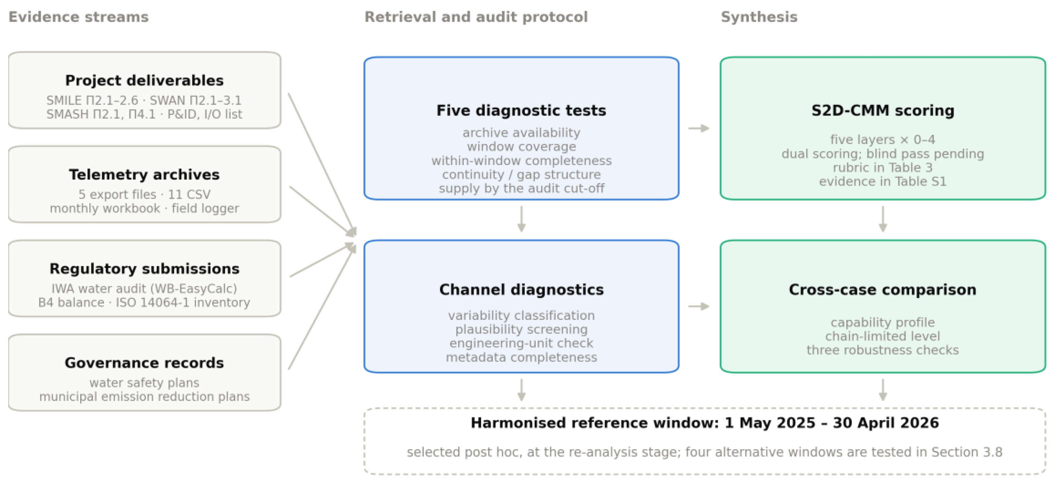
Figure 2.
Physical characteristics of the three systems. Connection density differs by an order of magnitude, which has direct consequences for both instrumentation economics and loss-indicator interpretation (Section 3.9).
Figure 2.
Physical characteristics of the three systems. Connection density differs by an order of magnitude, which has direct consequences for both instrumentation economics and loss-indicator interpretation (Section 3.9).
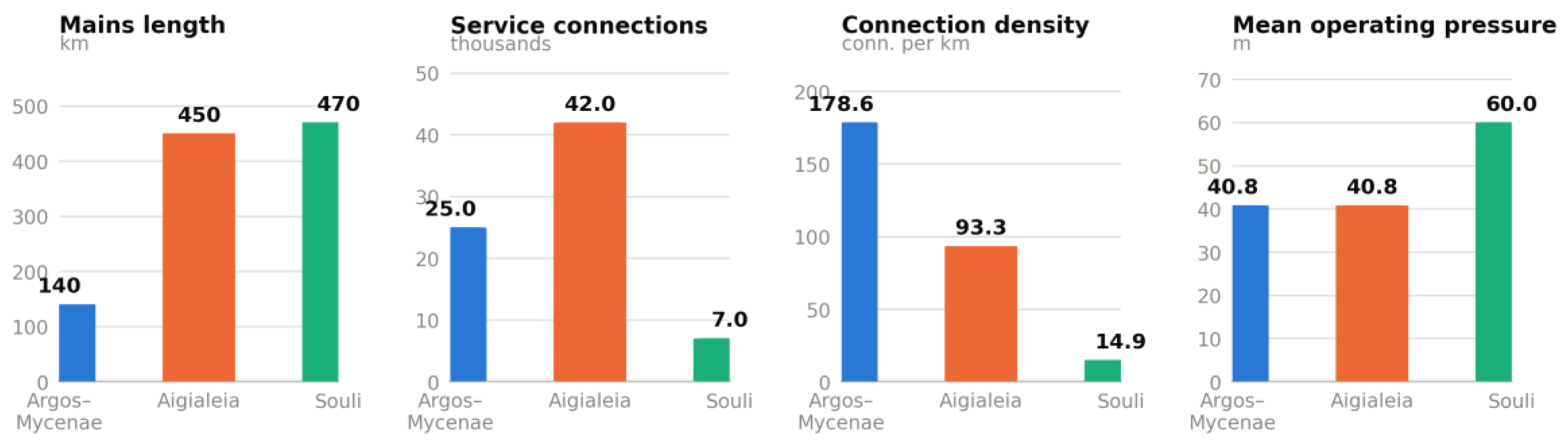
Figure 3.
Layer-by-layer assessment of the three deployments, with the chain-limiting layers marked. Each column reports the capability profile of one utility; the red rule marks every layer at that utility’s minimum.
Figure 3.
Layer-by-layer assessment of the three deployments, with the chain-limiting layers marked. Each column reports the capability profile of one utility; the red rule marks every layer at that utility’s minimum.
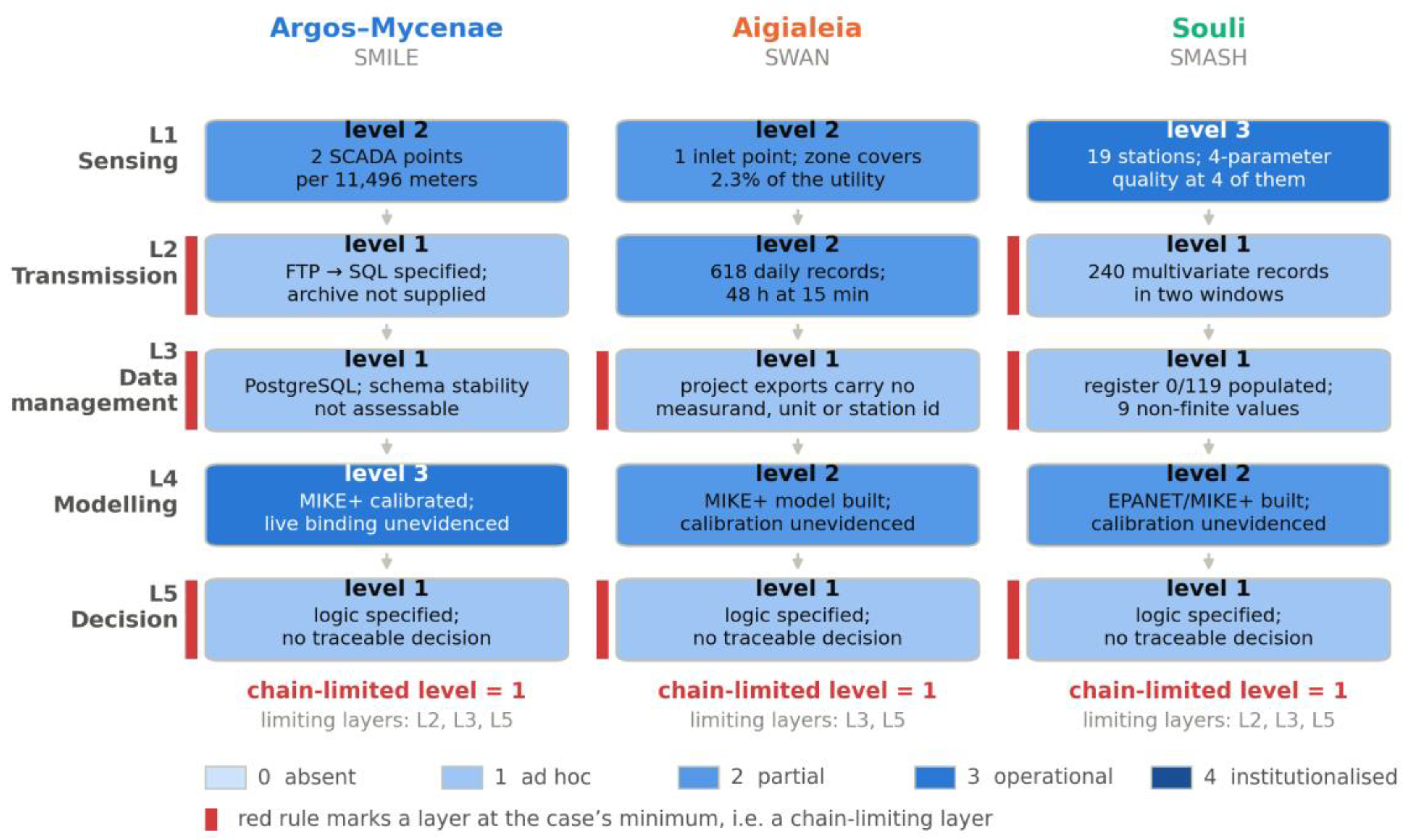
Figure 4.
Archive-level audit of the seven archives examined, six of which were supplied and one of which was requested but not supplied by the audit cut-off. The legend distinguishes three negative outcomes that are often conflated: failing a test is a property of the archive, non-supply is a property of the audit, and not assessable marks a test that could not be applied at all because the archive did not arrive.
Figure 4.
Archive-level audit of the seven archives examined, six of which were supplied and one of which was requested but not supplied by the audit cut-off. The legend distinguishes three negative outcomes that are often conflated: failing a test is a property of the archive, non-supply is a property of the audit, and not assessable marks a test that could not be applied at all because the archive did not arrive.
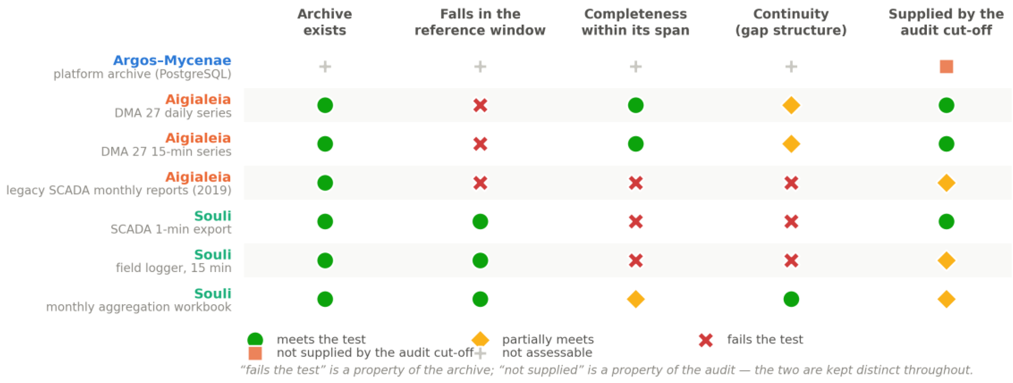
Figure 5.
Calendar coverage of every archive retrieved, with the reference observation window shaded. No calendar interval contains sub-hourly data from more than one utility.
Figure 5.
Calendar coverage of every archive retrieved, with the reference observation window shaded. No calendar interval contains sub-hourly data from more than one utility.
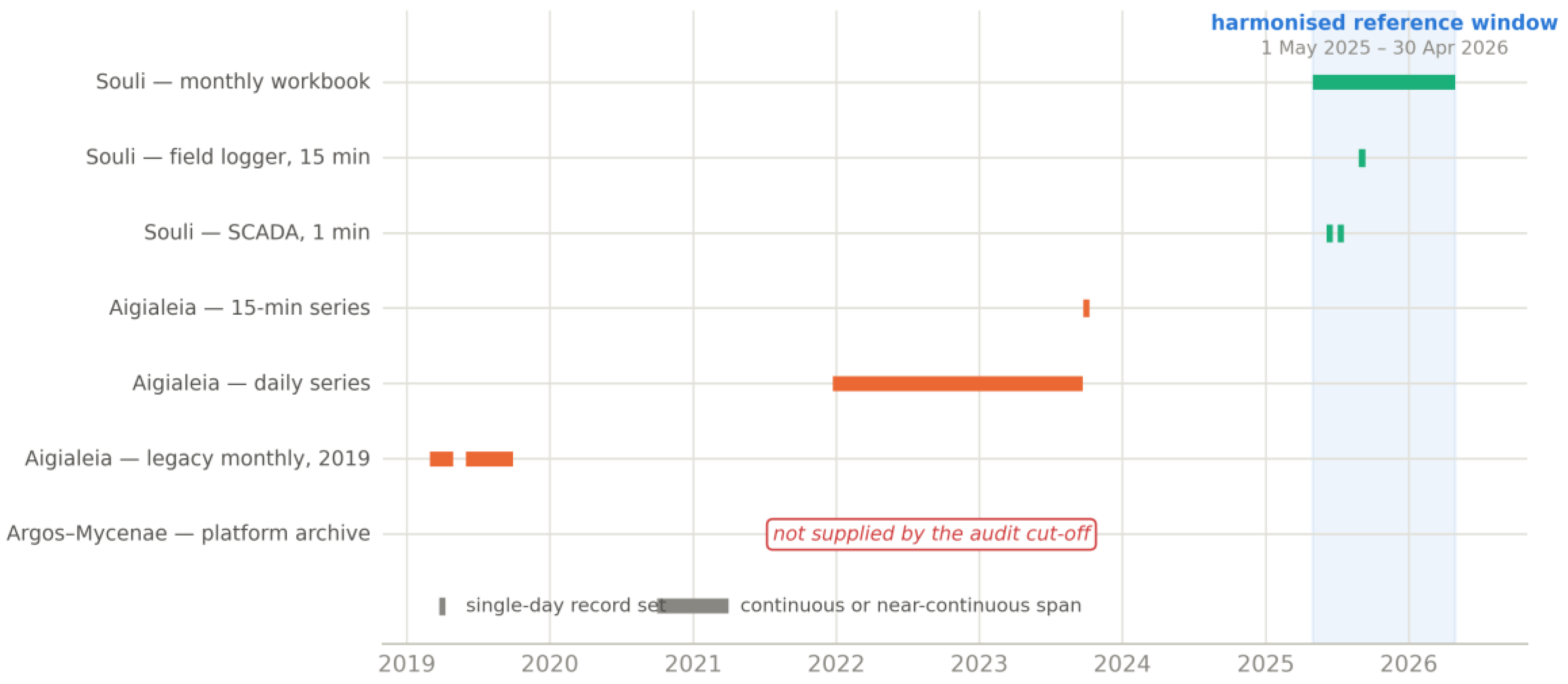
Figure 7.
Water-quality evidence from Souli. (a) The complete retrievable field-logger record: eight readings across two days in September 2025. (b) pH as stored by the supervisory export at four stations, against the field-logger readings and the admissible range for drinking water. The two sources are not synchronous and co-location is not established; the comparison identifies an inconsistency, it does not resolve it.
Figure 7.
Water-quality evidence from Souli. (a) The complete retrievable field-logger record: eight readings across two days in September 2025. (b) pH as stored by the supervisory export at four stations, against the field-logger readings and the admissible range for drinking water. The two sources are not synchronous and co-location is not established; the comparison identifies an inconsistency, it does not resolve it.
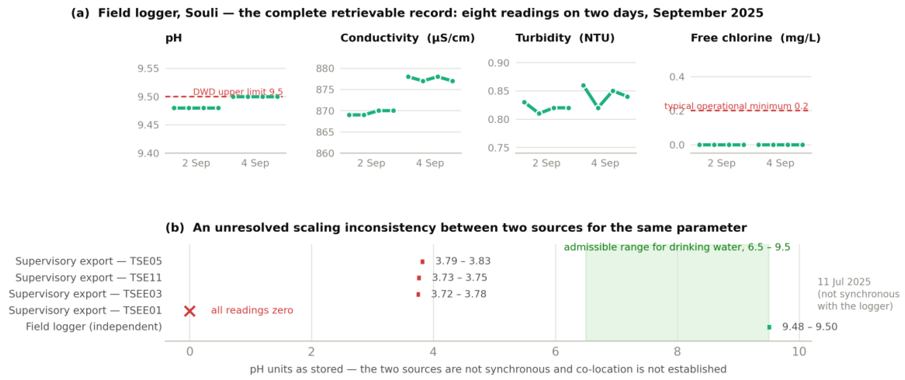
Figure 8.
(a) Capability profile of each deployment; the red rule marks every chain-limiting layer. (b) Capability-threshold requirements analysis: what would have to change, per case, for the chain-limited level to reach 2. (c) Reference-window sensitivity: transmission scores and chain-limited level under four candidate reference windows.
Figure 8.
(a) Capability profile of each deployment; the red rule marks every chain-limiting layer. (b) Capability-threshold requirements analysis: what would have to change, per case, for the chain-limited level to reach 2. (c) Reference-window sensitivity: transmission scores and chain-limited level under four candidate reference windows.
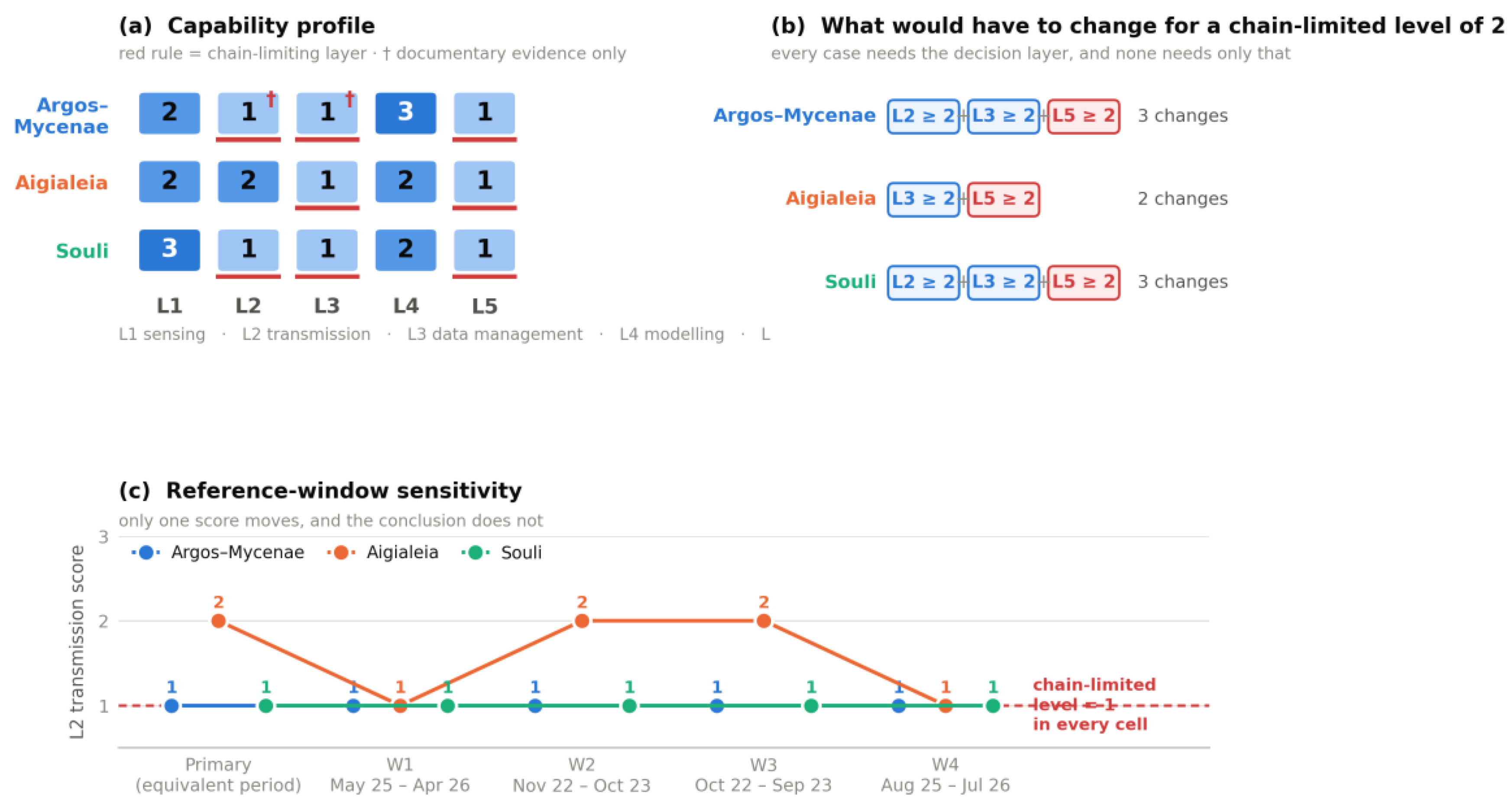
Figure 10.
(a) Decomposition of the unavoidable annual real losses allowance into its three constituent terms. (b) The resulting index against connection density. With three cases no functional relationship can be estimated; the panel shows that in these three utilities the index is strongly associated with connection density.
Figure 10.
(a) Decomposition of the unavoidable annual real losses allowance into its three constituent terms. (b) The resulting index against connection density. With three cases no functional relationship can be estimated; the panel shows that in these three utilities the index is strongly associated with connection density.
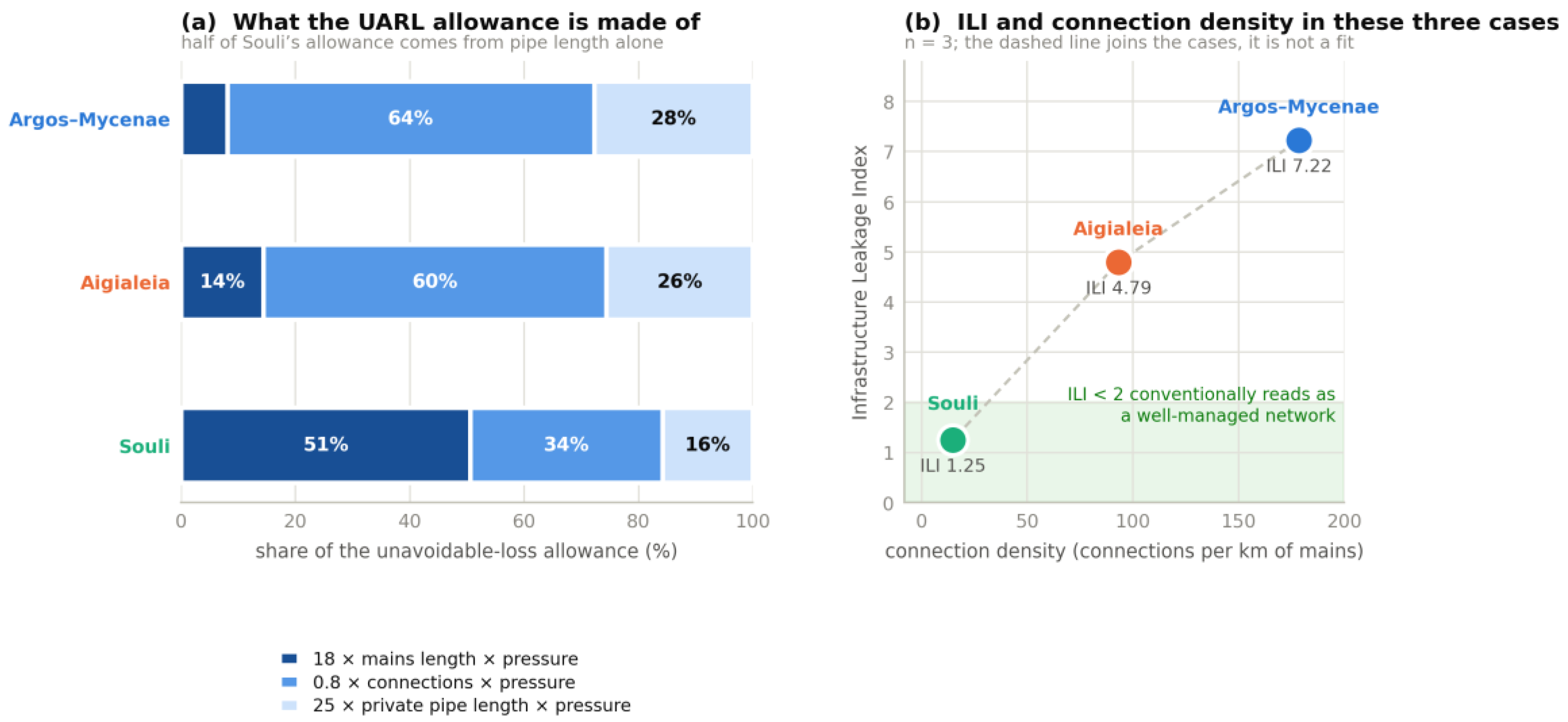

Table 1.
Characteristics of the three case-study water systems. Reporting years differ because they are the most recent years for which each utility completed a full water audit.
Table 1.
Characteristics of the three case-study water systems. Reporting years differ because they are the most recent years for which each utility completed a full water audit.
| Characteristic | Argos–Mycenae | Aigialeia | Souli |
|---|---|---|---|
| Utility type | Municipal water enterprise | Municipal water enterprise | Municipality |
| Region | Peloponnese | Western Greece | Epirus |
| Setting | Coastal plain | Coastal, linear | Mountainous, dispersed |
| Reporting year | 2023 | 2023 | 2025 |
| Total mains length (km) | 140 | 450 | 470 |
| — external / internal (km) | 40 / 100 | 100 / 350 | 190 / 280 |
| Service connections | 25,000 | 42,000 | 7,019 |
| Consumers served | 40,000 | 60,000 | 11,200 |
| Connection density (conn./km) | 178.6 | 93.3 | 14.9 |
| Mean operating pressure (m) | 40.8 | 40.8 | 60.0 |
| Supply hours (h/day) | 23.4 | 23.4 | 24.0 |
| Source mix (%) | 64.4 surface / 31.9 groundwater / 3.8 desalination | 38.1 surface / 61.9 groundwater | 85.0 surface / 15.0 groundwater |
| Mean tariff (€/m³) | 1.38 | 1.39 | 0.93 |
| Variable production cost (€/m³) | 0.33 | 0.32 | 0.20 |
| Annual operating cost (€) | 4,659,000 | 10,964,970 | 1,255,127 |
Table 2.
Comparative configuration of the three deployments, as specified in project documentation. Entries marked “not evidenced” mean that the feature is absent from the documents retrieved, not that it is known to be absent.
Table 2.
Comparative configuration of the three deployments, as specified in project documentation. Entries marked “not evidenced” mean that the feature is absent from the documents retrieved, not that it is known to be absent.
| Dimension | SMILE (Argos–Mycenae) | SWAN (Aigialeia) | SMASH (Souli) |
|---|---|---|---|
| Pilot zone | District metered area 1, three sub-zones | District metered area 27 | Paramythia closed zone, three pressure zones |
| Meters in pilot zone | 11,496 active | 973 active (13,664 utility-wide) | 7,019 connections municipality-wide |
| Zone assets | 136 full-control and 2 flow-control valves; ground elevations 2–76 m | 14 flow-control and 1 pressure-control valve in zone | 181 nodes, 7 reservoirs (248.0–403.4 m), ~24 km mains, DN60–DN200 |
| Pre-existing instrumentation | 2 SCADA flow/pressure points | 1 SCADA point at zone inlet | legacy municipal telemetry |
| Additional instrumentation specified | 7 flow/pressure sensors | 4 flow/pressure sensors | 19 remote stations, 1,347 I/O points |
| Water-quality instrumentation | none in pilot zone | none in pilot zone | chlorine and pH at 9 stations; chlorine, pH, turbidity and conductivity at 4 |
| Controllers | — | — | ABB AC500 / S500 |
| Actuation | — | — | 439 variable-frequency-drive signals; 128 chlorination dosing signals |
| Hydraulic model | MIKE+, calibrated against a SCADA demand pattern | MIKE+ on an EPANET 2.0 engine | EPANET / MIKE+ |
| Communications specified | NB-IoT, Sigfox, LoRaWAN, 2G–4G | NB-IoT, Sigfox, LoRaWAN, 2G–4G | cellular router; field data loggers |
| Persistence | FTP ingestion into PostgreSQL on a cloud server | SQL backend with a three-view web application | logger CSV; monthly aggregation workbook |
| Live model coupling | documented in deliverable Π2.6 | not evidenced | not evidenced |
| Decision logic | baseline model versus live measurement, deviation flagging | visualisation of hydrometers, supply meters and electricity meters | IWA water balance; NRW, apparent and real losses, UARL, ILI |
Table 3.
S2D-CMM scoring rubric. Each cell states the condition that must hold for the level to be awarded; a level requires all conditions of the levels below it.
Table 3.
S2D-CMM scoring rubric. Each cell states the condition that must hold for the level to be awarded; a level requires all conditions of the levels below it.
| Level | L1 Sensing | L2 Transmission | L3 Data management | L4 Modelling | L5 Decision integration |
|---|---|---|---|---|---|
| 0 | No permanent instrumentation in the assessed zone | No archive exists | No persistent store | No network model | No decision logic specified |
| 1 | Fewer than 1 permanent monitoring point per 10,000 connections in the instrumented zone, hydraulic parameters only | Sub-hourly records cover <1% of the assessment period, or the archive was not supplied by the audit cut-off | Store exists, but the level-2 conditions are not all positively evidenced—either because at least one of the following is present (schema instability within a reporting period; physically implausible or non-finite stored values; instrument metadata register absent or unpopulated) or because one of them cannot be assessed | Network geometry only (GIS or asset register), no hydraulic solver | Decision logic specified in documentation; no decision traceable to system output |
| 2 | 1 point per 1,000–10,000 connections in the instrumented zone, hydraulic parameters only | Sub-hourly records cover 1–50% of the assessment period, or records at daily resolution or finer cover ≥50% of it | Store, stable schema and documented sensor-to-asset mapping; no documented validation rules | Solver-based hydraulic model of the assessed zone, built and documented; calibration against measured data not evidenced | At least one documented operational or planning decision traceable to system output |
| 3 | The level-2 density band or better, and either better than 1 point per 1,000 connections or ≥2 water-quality parameters at ≥1 point | Sub-hourly records cover >50% of the assessment period, with gaps documented | As level 2 plus documented validation rules and a populated metadata register giving measurand and unit for every tag | Model calibrated against measured data, with the calibration source and period documented | Routine documented use with responsibility assigned to a named role |
| 4 | As level 3 plus documented calibration records and a fully populated instrument register | Sub-hourly records cover >95% of the assessment period, with a documented gap-handling procedure | As level 3 plus retention, versioning and audit-trail policy | Model bound to a live data source with evidence of the binding in operation, or automated state estimation | Institutionalised, with a periodic review cycle |
Table 4.
S2D-CMM scores against the Table 3 rubric. Scores marked † rest on documentary evidence that could not be corroborated against operating data.
Table 4.
S2D-CMM scores against the Table 3 rubric. Scores marked † rest on documentary evidence that could not be corroborated against operating data.
| Layer | Argos–Mycenae | Aigialeia | Souli |
|---|---|---|---|
| L1 Sensing | 2 | 2 | 3 |
| L2 Transmission | 1 † | 2 | 1 |
| L3 Data management | 1 † | 1 | 1 |
| L4 Modelling | 3 | 2 | 2 |
| L5 Decision integration | 1 | 1 | 1 |
| Capability profile | (2,1,1,3,1) | (2,2,1,2,1) | (3,1,1,2,1) |
| Chain-limited level | 1 | 1 | 1 |
Table 5.
Transmission-layer scores and chain-limited level under four candidate reference windows. The primary scoring uses the equivalent-period allowance described in Section 2.5, which is the most favourable treatment available to each archive; the four windows apply a single fixed calendar period to all three cases, which is the least favourable.
Table 5.
Transmission-layer scores and chain-limited level under four candidate reference windows. The primary scoring uses the equivalent-period allowance described in Section 2.5, which is the most favourable treatment available to each archive; the four windows apply a single fixed calendar period to all three cases, which is the least favourable.
| Window | Period | Rationale for the candidate | Argos L2 | Aigialeia L2 | Souli L2 | Chain-limited level |
|---|---|---|---|---|---|---|
| Primary | equivalent period per archive | most favourable treatment of each archive | 1 | 2 | 1 | 1, 1, 1 |
| W1 | 1 May 2025—30 Apr 2026 | the only window containing both sub-hourly telemetry and a complete annual record | 1 | 1 | 1 | 1, 1, 1 |
| W2 | 1 Nov 2022—31 Oct 2023 | contains the longest continuous daily series and one sub-hourly block | 1 | 2 | 1 | 1, 1, 1 |
| W3 | 1 Oct 2022—30 Sep 2023 | maximises coverage of the longest continuous daily series | 1 | 2 | 1 | 1, 1, 1 |
| W4 | 1 Aug 2025—31 Jul 2026 | most recent complete twelve months before the audit | 1 | 1 | 1 | 1, 1, 1 |
Table 6.
Recomputed performance indicators. Dashes denote variables not populated in that utility’s submission for that year. Ranges span the admissible sources described above.
Table 6.
Recomputed performance indicators. Dashes denote variables not populated in that utility’s submission for that year. Ranges span the admissible sources described above.
| Indicator | Argos–Mycenae (2023) | Aigialeia (2023) | Souli (2025) |
|---|---|---|---|
| System input volume (m³/yr) | — | — | 1,287,740 |
| Authorised consumption (m³/yr) | — | — | 778,330 |
| — of which billed (m³/yr) | — | — | 765,830 |
| — of which unbilled (m³/yr) | — | — | 12,500 |
| Apparent losses (m³/yr) | — | — | 69,480 |
| Real losses (m³/yr) | — | — | 439,930—455,849 |
| Real losses (% of system input) | — | — | 34.2—35.4 |
| Non-revenue water (m³/yr) | — | — | 521,910—527,300 |
| Non-revenue water (% of system input) | — | — | 40.5—40.9 |
| Unavoidable annual real losses (m³/day) | 1,271.1 | 2,287.6 | 1,002.4 |
| Infrastructure Leakage Index | 7.22 | 4.79 | 1.20—1.25 |
| Real losses (L/connection/day) | 375.7 | 267.3 | 171.7—177.9 |
| Real losses (L/connection/day/m pressure) | 9.21 | 6.55 | 2.86—2.97 |
| Water-supply electricity (kWh/yr) | — | — | 1,995,369 |
| Energy intensity of supply (kWh/m³) | — | — | 1.55 |
| Grid emission factor (g CO₂/kWh) | — | — | 367.51 |
| Carbon intensity of supplied water (kg CO₂e/m³) | — | — | 0.569 |
| Carbon intensity if energy not disaggregated (kg CO₂e/m³) | — | — | 1.241 |
| Emissions attributable to real losses (t CO₂e/yr) | — | — | 250.5–259.6 |
| Variable cost of real losses (€/yr) | — | — | 87,986–91,170 |
| Gross tariff-equivalent value of NRW (€/yr) | — | — | 485,376–490,389 |
Disclaimer/Publisher’s Note: The statements, opinions and data contained in all publications are solely those of the individual author(s) and contributor(s) and not of MDPI and/or the editor(s). MDPI and/or the editor(s) disclaim responsibility for any injury to people or property resulting from any ideas, methods, instructions or products referred to in the content. |
© 2026 by the authors. Licensee MDPI, Basel, Switzerland. This article is an open access article distributed under the terms and conditions of the Creative Commons Attribution (CC BY) license (http://creativecommons.org/licenses/by/4.0/).
Copyright: This open access article is published under a Creative Commons CC BY 4.0 license, which permit the free download, distribution, and reuse, provided that the author and preprint are cited in any reuse.