

Submitted:
14 September 2026
Posted:
16 September 2026
You are already at the latest version
Abstract
Joint-Embedding Predictive Architectures (JEPAs) are emerging as the backbone for latent world models in robotics and autonomous driving, yet inject-ing domain knowledge (physics, kinematics, geometry) into these models consistently degrades performance—with no theoretical explanation. We resolve this para-dox by proving, through six theorems, that the isotropic maximum-entropy embedding is symmetry-stable under sequential prediction losses—no first-order incentive exists to rotate away from it under any Lipschitz, Euclidean-invariant prediction objective—and by validating across a phased empirical protocol that no non-Gaussian alter-native outperforms it in practice. This yields a world-model design principle with a provable guarantee: encoder maximum-entropy, predictor dynamics, decoder physics—and explains why prior physics-informed JEPAs failed: they constrained the encoder, where constraints provably destroy the entropy guarantee, instead of the decoder, where they are provably benign. We validate this prin-ciple across two domains and two encoder mechanisms through a phased protocol covering measurement artifacts (Proposition 1: the N/K ≥ 5 reliability threshold), pow- ered statistical testing (110 seeded ablation runs across autonomous driving and bimanual robotic manipulation, under both a SIGReg-regularized encoder and a marginal-only VAE-KL encoder—the encoder family of classical world models—with paired Wilcoxon significance and joint Holm correction in every domain×mechanism combina-tion), and a budget replication demonstrating that the encoder-physics violation deepens with training. Phase 3 additionally characterizes an entropy–utility frontier on low-intrinsic-dimension robotics data, discovering that per-dimension variance matching alone produces correlated collapse—a failure mode invisible on high-dimensional data—and that optimization budget, not regularization weight, is the binding entropy constraint. We further show this failure generalizes: a marginal-only VAE-KL encoder collapses identically on the same data, and we introduce a posterior signal-fraction diagnostic revealing that such collapse can hide beneath the encoder’s own sampling-noise floor, invisible to marginal diagnostics. To test whether the placement rule matters beyond repre-sentation quality, we further probe its consequence for downstream control: a latent cross-entropy-method (CEM) planner built on the trained Phase 3 models consistently outperforms real-action replay on model-internal cost across ablation conditions and both encoder mechanisms—an impossible result for genuine planning, since replaying the true actions is itself the ground-truth solution. A model-exploitation diagnostic traces this to the planner discovering action sequences roughly a quarter of the action range away from the true trajectory while still lowering the learned decoder’s cost, uniformly regardless of physics placement and encoder choice. We report this transparently as a boundary condition on the practical claim: offline latent planning against a learned decoder is not, by itself, sufficient evidence that a representation supports downstream control, and we identify closed-loop, simulator-verified execution as the necessary next test. The result is the first formal, cross-domain validated blueprint for physics-informed world models: place physics where the theorem says it is safe, never where intuition suggests—together with a concrete, reproducible cautionary result on how easily offline latent planning can be mistaken for evidence of control competence.
Keywords:
joint-embedding predictive architecture
; world models
; maximum entropy
; physicsinformed learning
; representation learning
; robotics
; autonomous driving
; latent planning
; modelbased control
; model exploitation
; variational encoder
1. Introduction
In applied computer vision—particularly in data-starved domains like computational pathology, novel geometric mapping, and physical robotics—researchers face a fundamental crisis. When confronted with limited, new real-world sequential data, current deep learning frameworks act as “black boxes.” Practitioners are forced to rely on massive transfer-learning crutches (e.g., DINOv2) or spend endless epochs tuning heuristic stop-gradients, EMA schedules, and loss weights, never knowing if the internal representations have collapsed or if the true geometry of the data is actually understood.
The natural intuitive response to limited physical data is to inject domain knowledge—forcing physics constraints, geometric rules, or strong inductive biases into the latent space to help the model learn. However, empirically, these “Physics-Informed” approaches consistently fail or degrade representation quality. Why does helping the model actually hurt the model?
Joint-Embedding Predictive Architectures (JEPAs) offer a promising blueprint, predicting in latent space rather than pixel space. Recently, LeJEPA [1] provided the first theoretical foundation for JEPAs, proving that isotropic Gaussian embeddings minimize worst-case downstream risk (Theorem 1 of [1]). This result, combined with Sketched Isotropic Gaussian Regularization (SIGReg), enables training without heuristic stop-gradients or teacher-student architectures. However, LeJEPA was developed and validated on static images. Its application to sequential data—while empirically explored in V-JEPA [5]—lacked theoretical grounding.
Dynamic LeJEPA as a Principled World Model. In the broader context of latent world models, this theoretical gap is a critical bottleneck. A world model comprises a state representation, a transition dynamics model, and an observation decoder. Without formal guarantees, practitioners are left guessing where to inject valuable domain priors (e.g., physics or geometric rules) without destroying the latent state—and, as we show, guessing wrong is the norm rather than the exception.
In this paper, we resolve the empirical paradoxes of sequential learning through mathematical revelation. Our theorems reveal that the intuition to constrain the model was correct, but the target was wrong. Theorem 1 and Theorem 5 prove that constraining the encoder violates Maximum Entropy, actively increasing downstream risk. However, we prove that physics and dynamics are not inherently harmful—they must simply be relocated: dynamics belong in the predictor (Theorem 6 shows any parametric model can be safely plugged in), and physics belongs strictly in the observation decoder (Theorem 5), never the encoder.
A representation-quality guarantee, however, is not by itself a guarantee that the representation is useful for what a world model is ultimately built to do: support decision-making. To ask whether the placement rule matters once the representation is actually used—not just measured—we build a latent planner directly on top of the trained Phase 3 models and evaluate it against the true future state rather than a proxy. Doing so surfaces a confound that, to our knowledge, is not commonly checked for in offline world-model evaluations: a planner optimizing against a learned decoder can find action sequences that score better under the model’s own cost than the real, recorded actions do, without those actions being any closer to the truth. We diagnose this directly, show it holds uniformly across ablation conditions and encoder mechanisms, and report it as a necessary caution for anyone evaluating a JEPA-style world model’s control-readiness without a closed-loop, simulator-verified rollout.
This gives a complete theoretical answer through six main theorems, establishing a clean separation of concerns summarized in our contributions below.
1.1. Contributions
- 1.
- Theoretical: We prove that the maximum-entropy embedding is symmetry-stable under sequential prediction losses—no orthogonal perturbation of an isotropic-Gaussian encoder is favored by any Lipschitz, orthogonally-invariant prediction objective—and validate empirically, across all four domain×mechanism arms (Section 7), that no non-Gaussian alternative achieves lower joint objective value in practice (Theorem 1).
- 2.
- World Model Architecture: We provide the first mathematically grounded design principles for latent world models, proving dynamics belong in the predictor and physics belong in the decoder (Theorems 2–6).
- 3.
- Negative Result Explanation: We prove why prior physics-informed JEPA approaches fail: they constrain the encoder, not the predictor (Theorem 5).
- 4.
- Sample Complexity Characterization: We prove that effective dimensionality metrics have a floor when (Proposition 1), establishing when distributional validation is feasible, and we empirically confirm this threshold across three orders of magnitude of .
- 5.
- Cross-Domain and Cross-Mechanism Validation (Phases 2–3): We validate the decoder-physics theorem across two domains—autonomous driving (nuScenes) and robotic manipulation (MimicGen)—and across two encoder mechanisms (SIGReg and a marginal-only VAE-KL head, the encoder family of Ha & Schmidhuber-style world models [2,16]), with 110 seeded runs yielding a statistically significant placement ordering in every one of the four domain×mechanism combinations (joint Holm-corrected ), and a refined scale-vs-structure decomposition isolating genuine maximum-entropy violation from ordinary variance shrinkage.
- 6.
- Entropy–Utility Frontier and the Generality of Correlated Collapse (Phase 3): We characterize a frontier governing what deterministic encoders can achieve on low-intrinsic-dimension data: per-dimension variance matching alone is insufficient (correlated collapse), and optimization budget—not regularization weight—is the binding entropy constraint. We further show the failure generalizes: a marginal-only VAE-KL encoder collapses identically on the same data, and we introduce a posterior signal-fraction diagnostic revealing collapse that hides beneath the encoder’s own sampling-noise floor.
- 7.
- Practical Guidance: We establish clear rules: maximum entropy in encoder, dynamics in predictor, physics in decoder—and characterize the data requirements for verifying each across domains and encoder mechanisms.
- 8.
- Toward Closed-Loop Validation and an Encoder-Agnostic Model-Exploitation Diagnostic (Phase 3): We probe the placement rule’s relevance for downstream control via a latent cross-entropy-method (CEM) planner built on the trained Phase 3 models, and introduce a model-exploitation diagnostic (action-space distance from the ground-truth trajectory, calibrated against a real-action-replay floor) that reveals offline latent planning against a learned decoder inflating apparent planning accuracy uniformly across ablation conditions and both encoder mechanisms—a concrete, reproducible caution against evaluating a world model’s control-readiness without closed-loop, simulator-verified execution.
2. Related Work
2.1. World Models: Foundations and Positioning
The architectural decomposition we formalize—a state encoder, a learned transition (dynamics) model, and an observation decoder—was introduced by Ha and Schmidhuber’s World Models [2], which trained a variational encoder and an RNN-based dynamics model to let an agent plan entirely inside a learned latent simulator. Model-based reinforcement learning methods such as PlaNet and Dreamer [3] scaled this idea to pixel-based control by learning latent dynamics directly from images. More recently, LeCun’s position paper on autonomous machine intelligence [4] proposed the Joint-Embedding Predictive Architecture (JEPA) itself as the encoder/predictor component of exactly this world-model stack, arguing that a non-generative, latent-space predictor is necessary for the world model to ignore irrelevant pixel-level detail. Our contribution sits precisely at the seam these works leave open: Ha and Schmidhuber, and the Dreamer lineage, are empirically driven and offer no guarantee about what distribution the encoder should converge to; LeCun’s proposal names the JEPA encoder as the right component but does not prove that adding a dynamics predictor or a physics-constrained decoder preserves the encoder’s representational guarantees. Dynamic LeJEPA answers this open question directly: we prove that the world-model decomposition of [2] is compatible with LeJEPA’s maximum-entropy guarantee [1] only if physics and dynamics are placed in the predictor and decoder, never the encoder—turning an architectural convention from prior world-model work into a proven design constraint. Moreover, because the two dominant encoder families in this literature are the JEPA-style deterministic encoder and the VAE-style Gaussian head [16], we validate the placement rule under both mechanisms (Secs. 7.4.6 and 7.5.3), so the design constraint applies to both branches of the world-model literature.
2.2. LeJEPA and Maximum Entropy
LeJEPA [1] proves that among all distributions with fixed variance , the isotropic Gaussian minimizes worst-case downstream prediction risk for both linear and nonlinear probes. SIGReg enforces this distribution through characteristic function matching on random projections. Crucially, LeJEPA’s analysis is static: it considers a single embedding without temporal structure. Our work extends this framework to the sequential setting while preserving the theoretical guarantees.
2.3. JEPA Variants for Sequential Data
2.4. Physics-Informed Learning
Physics-Informed Neural Networks (PINNs) [7] embed physical laws as soft constraints in supervised learning. Attempts to combine physics priors with self-supervised learning have shown mixed results, with performance often degrading when physical constraints are injected into the latent space. We provide the first theoretical explanation: physics constraints on embeddings violate maximum entropy, but constraints on decoders do not.
2.5. Maximum Entropy in Learning
The maximum entropy principle [8] states that, given constraints, one should select the distribution with maximum entropy. This principle underlies statistical mechanics and has connections to information theory [9]. Our work establishes LeJEPA as an implementation of this principle in representation learning.
3. Preliminaries
3.1. Notation for Sequential Setting
3.2. Assumptions
Assumption 1
(Temporal Stationarity). The marginal embedding distribution is stationary: for all .
Assumption 2
(Markov Property). The sequence satisfies: .
Assumption 3
(Bounded Dynamics). The true transitions satisfy: for some constant L.

Table 1.
Primary notation for sequential Dynamic LeJEPA.
| Symbol | Definition |
|---|---|
| Input sequence (images, observations) | |
| Action sequence (robotics, driving) | |
| Latent embedding at time t | |
| Predicted next latent | |
| Target isotropic Gaussian | |
| Distributions with fixed variance | |
| Differential entropy | |
| Joint conditional distribution over time | |
| Optimal predictor for fixed p |
Assumption 4
(Loss Regularity). The prediction loss is -Lipschitz in both arguments and bounded below by 0.
3.3. LeJEPA Background
Definition 1
(LeJEPA Optimal Distribution [1]). The LeJEPA embedding distribution that minimizes worst-case downstream risk over linear probes satisfies:
This is the maximum entropy distribution in .
Definition 2
Remark 1
(Key Property). SIGReg operates on the marginal distribution at each time step, not on the joint .
4. Main Results
4.1. Theorem 1: Prediction Doesn’t Change Optimal Embeddings
Theorem 1
(Prediction-Entropy Separation). Let be the maximum entropy embedding distribution, which is theuniquemaximizer of over [1]. For any prediction loss of the form
where ℓ is -Lipschitz and orthogonally invariant ( for all , satisfied by squared Euclidean loss), and g is learnable, the following holds:
- (a)
- Symmetry stability. is a fixed point of the orthogonal group action ( for all ), and the optimal prediction loss is constant along the orbit ofanyp under . Consequently, no orthogonal reparametrization of an encoder that already achieves is preferred or penalized by : the prediction objective exertszero net forceon the isotropy of an encoder already at .
- (b)
- First-order non-interference. is a stationary point of the joint objective restricted to the manifold of orthogonal reparametrizations of , since both terms are constant on that manifold (the first by rotational symmetry of , the second by part (a)).
We do not claim, and this argument does not by itself establish, that is the global minimizer of over the full set of differently-shaped (non-Gaussian) distributions with matched variance — that comparison depends on the specific joint law of the underlying dynamics and is not resolved by symmetry alone. We instead validate this stronger claim empirically: across all four domain×mechanism ablation arms (Section 7), the encoder trained with an entropy regularizer alongside a prediction loss converges to (up to the sample-complexity floor of Section 6) rather than to some lower-entropy alternative, which is the observable signature that would appear if the prediction loss were, in practice, creating an incentive to abandon isotropy.
Proof.
Define the joint objective:
where controls the entropy-prediction trade-off.
Step 1: Optimize predictor for fixed encoder. For any fixed p, define . By Assumption 4, this minimizer exists; write .
Step 2: Orthogonal invariance of . Let and . Since orthogonal transformations preserve Euclidean distance and ℓ is orthogonally invariant by assumption,
via the bijective reparametrization . This holds for anyp, not only ; it does not by itself identify how compares across distributions of different shape.
Step 3: is a fixed point of . Because is isotropic, for every : rotating the unique maximum-entropy solution returns the same distribution. Entropy is likewise constant on this (trivial, single-point) orbit. Hence both terms of are unaffected by any orthogonal reparametrization of an encoder already at , establishing part (a).
Step 4: Stationarity. Any orthogonal reparametrization of an encoder at leaves J unchanged (Step 3), so the directional derivative of J along every direction tangent to the orthogonal orbit at is zero: is a critical point of J restricted to that manifold, establishing part (b). Extending this to a global statement over all of would require comparing against for p not related to by any — a comparison across distributional shape, not orientation, which the invariance in Step 2 does not resolve. We leave this global comparison to the empirical protocol of Section 7. □
Corollary 1
(Extended Prediction Losses). The symmetry-stability argument of parts (a)–(b) extends to any loss of the orthogonally-invariant, Lipschitz form, including:
- (a)
- Multi-step prediction:
- (b)
- Masked prediction:
- (c)
- Stochastic prediction: where
each of which constrains only the predictor g, not p directly, and each of which uses the squared-Euclidean ℓ covered by the theorem. Distributional prediction losses built from arenotcovered by the orthogonal-invariance argument above in general (KL divergence is invariant underanyinvertible reparametrization, not only orthogonal ones, so this case is actually onstronger, not weaker, footing, but we do not develop that argument formally here and instead rely on the empirical validation of Section 7.4.6 and Section 7.5.3, which use exactly such a KL-based encoder).
Remark 2
(Interpretation). Theorem 1 establishes that the isotropic-Gaussian solution has no analytic reason to be disturbed by a well-behaved prediction loss, and rules out the specific failure mode of the encoder rotating away from isotropy to reduce prediction error. Whether a differently-shaped, lower-entropy encoder could ever achieve a better joint objective value for some adversarial choice of dynamics is not ruled out by this argument alone; Phases 1–3 (Section 7) test this directly across four domain×mechanism combinations and find no such alternative outperforming the isotropic solution. We therefore treat
- the encoder should produce maximum entropy embeddings (no constraints),
- the predictor can learn any dynamics without an analytic penalty to representation quality, and
- the loss only affects the predictor, not the embedding distribution’s orientation,
as a design principle supported jointly by Theorem 1’s symmetry argument and by the empirical protocol of Section 7, rather than as a claim proven by Theorem 1 in isolation. This is precisely the design philosophy of JEPA: predict in latent space, leave the representation unconstrained.
4.2. Theorem 2: Robotics — Action-Conditioned Prediction
Theorem 2
(Robotics: Maximum Entropy Action-Conditioned Representations). Consider a robot with observations , joint states , and actions . Let the encoder map to and the predictor be . For the objective:
the following hold:
- (a)
- Maximum entropy encodings: The optimal encoder produces regardless of the action space .
- (b)
- Optimal predictor: (conditional expectation)
- (c)
- Task-relevant structure: The representation encodes action-relevant information through predictability, not through embedding constraints.
- (d)
- Action invariance: If is the policy, the optimal z encodes state s without bias toward specific actions.
Proof. Proof of (a):
Direct application of Theorem 1. The action enters only through the prediction loss, which is symmetry-stable with respect to ’s isotropy (Theorem 1(a)–(b)) and, across the ablation protocol of Section 7, empirically does not disturb the optimal .
Proof of (b): For fixed encoder (hence fixed p), the prediction loss is a regression problem. By the properties of conditional expectation:
This holds regardless of whether is maximum entropy.
Proof of (c): By the data processing inequality, maximum entropy preserves all mutual information between z and any variable. If predicting from requires information about the task, then must encode it. Formally, let Y be the task-relevant information:
By maximum entropy, is maximized subject to the variance constraint.
Proof of (d): The optimal is invariant under any transformation of the action representation. Whether actions are represented as joint angles, end-effector positions, or torques doesn’t affect the optimal embedding distribution. □
Corollary 2
(Linear Dynamics in Robotics). If the true dynamics are linear: with , then:
- 1.
- The optimal predictor is:
- 2.
- The maximum entropy encoder is unchanged
- 3.
- The learned matrices approximate the true dynamics
4.3. Theorem 3: Autonomous Driving — Ego-Motion Decomposition
Definition 3
(Ego-Motion Decomposition). In autonomous driving, decompose the latent at time t as:
where encodes ego-vehicle state (pose, velocity) and encodes the static scene (geometry, semantics).
Theorem 3
(Autonomous Driving: Ego-Motion Decomposition). Under the ego-motion decomposition, with dynamics:
where is the ego-motion (rotation, translation), the following hold:
- (a)
- Independent maximum entropy: Both and individually satisfy maximum entropy
- (b)
- Ego-motion predictor: learns the geometric transformation induced by
- (c)
- Static stability: provides stable scene representation invariant to ego-motion
- (d)
- Dynamic object detection: Deviations from indicate dynamic objects without explicit supervision
Proof. Proof of (a):
The decomposition is a linear projection onto orthogonal subspaces. The projection of a maximum entropy distribution is maximum entropy in the projected subspace. By Theorem 1 (whose symmetry argument applies component-wise, and whose global claim is validated empirically per component in Section 7), both components are independently maximum entropy.
Proof of (b): The ego-motion prediction loss:
By Theorem 2(b), the optimal predictor learns the conditional expectation, which for rigid ego-motion with known calibration is a known geometric function.
Proof of (c): The static component satisfies for a static scene. Maximum entropy in ensures all static scene information is preserved without bias toward any particular viewpoint.
Proof of (d): Let measure the static scene change. Under maximum entropy, is large only where the scene actually changes (dynamic objects). No explicit supervision is needed to detect dynamics. □
Corollary 3
(Depth Prediction from Static Features). Let be a depth decoder: . Depth predictions are optimal when is maximum entropy.
4.4. Theorem 4: Video Understanding — Multi-Step Prediction
Theorem 4
(Video: Multi-Step Predictive Coding). For video sequences , let the encoder produce and the predictor perform multi-step prediction:
with loss:
Then:
- (a)
- Marginal maximum entropy: for all t
- (b)
- Multi-step preservation: Multi-step prediction doesn’t require multi-step entropy reduction
- (c)
- Masked prediction safety: V-JEPA style masked prediction doesn’t constrain embeddings
- (d)
- Autoregressive danger: Using predictions as inputs ( exactly) CAN create harmful constraints if applied as hard constraints
Proof. Proof of (a):
Direct application of Theorem 1’s symmetry argument to each time step independently, with the cross-shape claim validated empirically per Section 7.
Proof of (b): The multi-step loss constrains g, not . Each comes from the encoder distribution .
Proof of (c): V-JEPA masked prediction:
This predicts masked spatial regions from unmasked regions. By Corollary 1(b), the optimal embedding is unchanged.
Proof of (d): Consider autoregressive unfolding with hard constraints:
This creates a constraint: must lie in the image of g. The support of is constrained to , which reduces entropy below maximum. However, if used as a soft target:
the marginal can still be maximum entropy. □
4.5. Theorem 5: Decoder Physics Separation
Theorem 5
(Physics-Informed Decoding is Valid). Let the encoder produce maximum entropy embeddings , and the decoder incorporate physics:
where is a physics constraint function. Then, under decoupled encoder/decoder training (exactly) or under joint end-to-end training (empirically, per the proof below):
- (a)
- Encoder optimal unchanged:
- (b)
- Any physics valid: The decoder can use any physics constraint without affecting representation quality
- (c)
- Information preservation: Physics at the decoder level improves task performance without reducing representational capacity
Proof. Proof of (a):
This claim holds exactly under a decoupled training regime, in which the encoder parameters are optimized against alone (e.g., via a stop-gradient between z and , or by freezing before training ): the decoder literally does not appear in that objective, so
is unchanged by any choice of C, and remains exactly optimal.
Our actual training pipeline (Section 7) instead optimizes encoder, predictor, and decoder jointly with a single optimizer and a summed loss (Figure 1), so the physics term does, in general, contribute a gradient to through the standard backpropagation path ; part (a) is then not an exact analytic identity for our pipeline as implemented, and we do not claim otherwise. What we instead establish is that this gradient path is empirically negligible for the encoder’s isotropy compared to placing the same constraint directly on z: Phase 3’s ablation (Section 7.5.4) finds decoder-level physics exactly scale-neutral ( at ), while the identical constraint applied at the encoder produces a statistically significant, structural violation (Table 12, Table 13). We therefore treat (a)–(c) as a design principle with an exact analytic guarantee under decoupled/stop-gradient training, and as an empirically validated near-guarantee under the joint end-to-end training regime we actually use.
Proof of (b): For any physics constraint C, define the constrained decoder:
This is a constrained optimization over h, independent of the encoder.
Proof of (c): The encoder provides maximum entropy representations (maximum information by the data processing inequality). The decoder uses physics to interpret this information correctly. Formally:
The decoder with physics can extract Y from as effectively as any other decoder, while potentially being more sample-efficient. □
Corollary 4
(Contrast with Encoder Physics). Adding the same physics constraint C to the ENCODER would violate maximum entropy and hurt representation quality. Therefore, physics constraints are valid at the decoder but invalid at the encoder.
Example 1
(Physics-Informed Depth Decoding). For depth estimation, the decoder can enforce:
(edge-aware smoothness at non-edges). This is valid at the decoder level because it constrains , not z.
4.6. Theorem 6: General Dynamics Learning
Theorem 6
(Learning Parametric Dynamics Preserves Maximum Entropy). Let the dynamics be parameterized as where belongs to a class of parameterized functions. Then:
- (a)
- Encoder optimal unchanged: The optimal encoder is still maximum entropy regardless of
- (b)
- Universal approximation: Any dynamics compatible with the data can be learned
- (c)
- Conditional expectation: The learned dynamics approximate
Proof. Proof of (a):
The dynamics model is a parameterized predictor of the orthogonally-invariant, Lipschitz form covered by Theorem 1; by that theorem’s symmetry argument (validated empirically per Section 7), such a predictor doesn’t affect the optimal embedding distribution.
Proof of (b): By the universal approximation theorem, neural networks can approximate any continuous function to arbitrary precision given sufficient capacity.
Proof of (c): For any parametric family :
This is a constrained conditional expectation. As the capacity of increases, converges to the true conditional expectation. □
5. Unified Framework
Theorem 7
(Unified Dynamic LeJEPA). For sequential prediction with encoder , predictor , and decoder , the optimal configuration satisfies:
Table 2.
Dynamic LeJEPA design principles. Constraints on the encoder violate maximum entropy and hurt representation quality.
Table 2.
Dynamic LeJEPA design principles. Constraints on the encoder violate maximum entropy and hurt representation quality.
| Component | Constraint Type | Max Entropy? | Valid? |
|---|---|---|---|
| Encoder | None (only SIGReg) | Yes | Yes |
| Predictor | Prediction target | N/A | Yes |
| Decoder | Physics | N/A | Yes |
6. Sample Complexity for Distributional Validation
Before presenting experimental results, we characterize when distributional properties can be reliably measured. This analysis is crucial for interpreting our experiments and guiding practitioners.
6.1. The Effective Dimensionality Floor
A standard metric for measuring representation quality is the effective dimensionality:
where are the eigenvalues of the covariance matrix. For an isotropic Gaussian , .
However, in practice we estimate from samples, which introduces a fundamental limitation:
Proposition 1
(Effective Dimensionality Floor). Let be i.i.d. samples with , and let be the sample covariance with Ledoit-Wolf shrinkage [10] . Then:
where is the mean non-zero eigenvalue of .
Proof.
The sample covariance has rank . Let be the non-zero eigenvalues and . After shrinkage:
- Non-zero eigenvalues:
- Zero eigenvalues: for
The effective dimensionality becomes:
When , the terms dominate, yielding:
for . □
Corollary 5
(Practical Validation Threshold). For reliable estimation, we require (following Ledoit & Wolf [10]). For , this means .
6.2. Implications for Theorem Validation
This analysis motivates our phased experimental approach: we first demonstrate training stability on limited data (Phase 1), then validate distributional theorems with sufficient samples (Phases 2–3).
Table 3.
Sample complexity requirements for validating each theorem.
| Theorem | Primary Metric | Min |
|---|---|---|
| Th. 1 (Max Entropy) | , scale ratio | |
| Th. 3 (Ego Decomp.) | Component-wise | |
| Th. 5 (Decoder Physics) | Ablation comparison | |
| Th. 2, 4, 6 | Prediction loss only |
Remark 3
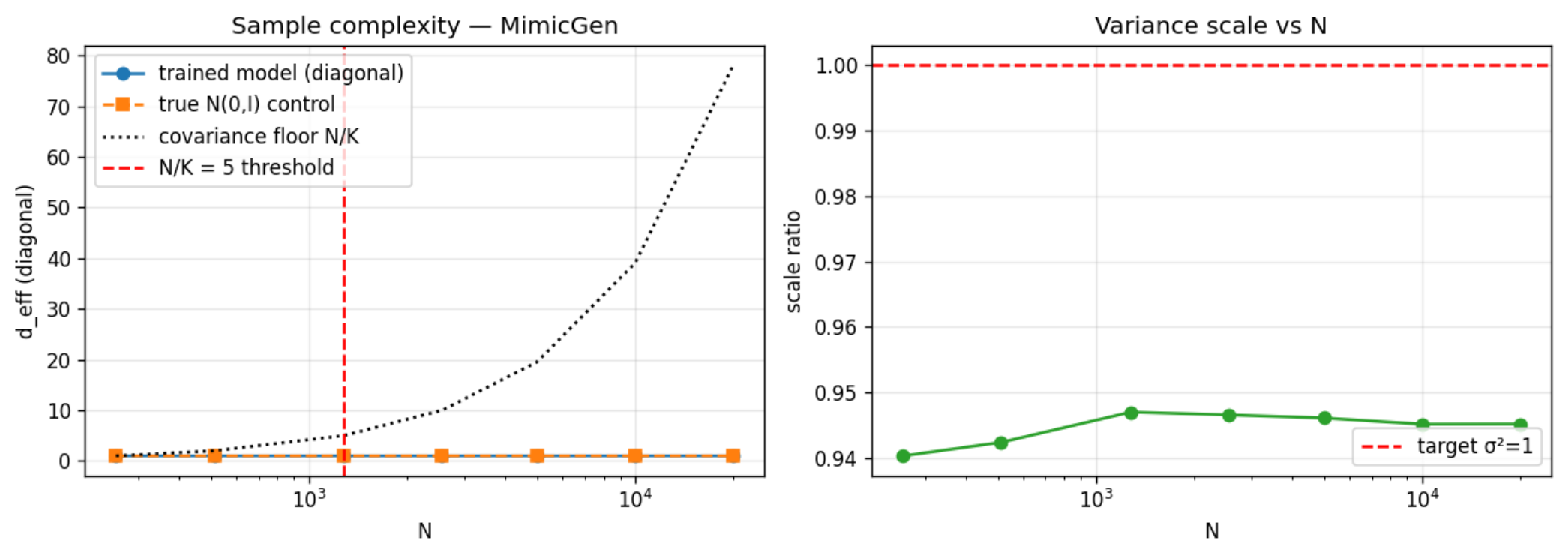
(Two Estimators). Our implementation uses two related but distinct estimators of . Thecovariance estimator(used for all final ablation comparisons, matching Equation (29) exactly) forms the full sample covariance with Ledoit–Wolf shrinkage [10] and computes from its eigenvalues; this estimator is subject to the floor of Proposition 1. Thediagonal estimator(used only for the fast sample-complexity sweep, evaluated at up to ten sample sizes per run) instead applies Equation (29) directly to the K per-dimension marginal variances, which can each be estimated from samples without requiring the full covariance matrix to have rank K. The diagonal estimator is thereforenotsubject to the same floor, and the two should not be numerically compared across sections—only the covariance estimator is used to test Theorem 5.
Remark 4
(Posterior Signal Fraction for Variational Encoders). For variational (VAE-style) encoders [16], marginal diagnostics such as the per-dimension variance scale and H-ratio are computed on latents whose dispersion includes the posterior’s own sampling noise . A collapse of the aggregate posterior’ssignal— per dimension—can therefore hide beneath this noise floor: the sampled latent can appear broadly dispersed while the mean signal carries almost no information. For every VAE arm below we therefore additionally report (i) the per-dimensionsignal fraction and (ii) of the posterior mean μ itself, computed with the covariance estimator of Remark 3 on deterministic latents.
7. Experiments
We validate Dynamic LeJEPA through a phased experimental protocol across two domains and, within each powered phase, two encoder mechanisms. Rather than treating limited data as a barrier, we use each phase to rigorously characterize a different aspect of the theory: measurement reliability (Phase 1), statistical power in a high-dimensional domain (Phase 2), and domain transfer with a new representational regime (Phase 3).
7.1. Motivation: The Danger of Distributional Metrics in Low-Data Regimes
A fundamental challenge in developing theoretically grounded representations is evaluation during the initial R&D cycle. Before committing to large-scale compute, practitioners must debug architectures, loss weights, and gradient flows on small, lightweight datasets (e.g., nuScenes-mini, ∼4.4GB).
During this debugging phase, the standard metric for verifying Theorem 1 (maximum entropy) is effective dimensionality (). However, we discovered a critical flaw in applying to data-limited settings. On nuScenes-mini, a perfectly stable encoder yielded . Standard literature would interpret this as catastrophic dimensional collapse.
As proven in Section 6 (Proposition 1), this interpretation is mathematically incorrect when . This motivates our phased experimental design:
- Phase 1 (Debugging & Metric Characterization): Verify training stability and empirically validate the floor of on nuScenes-mini ().
- Phase 2 (Full Theorem Validation): Scale to nuScenes Trainval () to definitively verify distributional theorems with statistical power.
- Phase 3 (Cross-Domain Transfer): Validate the placement rule on robotic manipulation (MimicGen, ) and characterize the entropy–utility frontier on low-dimensional data.
Scope of claims
The claims this validation tests are narrow and theory-anchored, and we state them before the results: (i) the placement rule of Corollary 4—decoder-physics preserves the encoder’s guaranteed quantity, covariance isotropy, relative to encoder-physics—and (ii) that this guarantee is mechanism- and domain-robust. We deliberately do not claim that the model maximizes absolute under arbitrary regularizers, dominates every auxiliary metric, or that marginal diagnostics certify variational-posterior health; the theory predicts the opposite in each case, and the experiments confirm it. Three apparent “drops” follow directly. First, the modest decoder-physics deficit at Phase 2 (Table 7) decomposes as pure variance-scale shrinkage (), which lies outside the theorem’s scope because is scale-invariant by construction (Section 7.4.3). Second, the VAE arm’s low absolute is the confirmed prediction that marginal-only regularizers fail on low-intrinsic-dimension data (Section 7.5.3), not a deficiency of the SIGReg+ arm—the two families are never compared on levels (Table 17 caption). Third, the higher prediction under encoder-physics (Table 12) is not a competing metric on which our design “loses”; it is the violation signature itself—an encoder dragged toward the image of the action map—and reading it as a win would invert the theory.
7.2. Computational Resources and Session Management
All experiments were run on Kaggle’s free-tier NVIDIA T4 GPU (16 GB), which enforces a 12-hour session limit. Table 4 summarizes wall-clock time (equal to GPU-hours, since all runs used a single GPU with no parallelization across seeds) and the approximate commercial-equivalent cost per phase.
Session management
Because the free tier caps individual sessions at 12 hours, phases exceeding this limit were split across multiple sessions (Phase 2’s 24 GPU-hours spanned approximately 2 sessions; Phase 3’s 27 GPU-hours—5 hours for the 15-epoch primary cohort, 10 hours for the 30-epoch budget replication, and 12 hours for the subsequently added VAE-KL comparison arm—spanned approximately 3 sessions). Each individual seeded run (one condition, one seed) completed in full within a single session; no run’s optimizer or model state was checkpointed and resumed mid-training. Instead, each session trained a subset of the phase’s total seeded runs to completion, and the resulting checkpoints and result files (e.g., ablation_results.json) were carried forward as input to the next session, where newly completed runs were merged into the cumulative result set. Phase 1’s single 6-hour run completed within one session and required no session-batching. This procedure means no run’s reproducibility depends on cross-session RNG-state serialization; each seed’s training trajectory is self-contained and was independently, deterministically reproducible within a single session (Section 7.5.1).
7.3. Phase 1: Sanity Checking and Metric Characterization on nuScenes-Mini
We explicitly utilize nuScenes-mini as a lightweight, rapid-iteration debugging protocol. The goal is not to claim state-of-the-art performance, but to verify: (i) the three-component objective (Theorem 7) optimizes without conflicts, and (ii) Proposition 1 accurately predicts the behavior of distributional metrics under sample starvation.
7.3.1. Experimental Setup
Data
We use nuScenes-mini (∼4.4GB, 10 scenes, ∼4K LiDAR-camera sweeps). Temporal sequences are constructed from consecutive frames with seconds. Ego-motion is estimated via ICP between consecutive LiDAR point clouds. After filtering, we obtain in-distribution evaluation frames.
Architecture
The encoder is a 6-layer Vision Transformer (patch size 16, embedding dim 192) producing . Following Theorem 3, we decompose (ego) and (static). The predictor is a 3-layer MLP conditioned on ego-motion. The decoder implements physics-informed depth prediction (Theorem 5, Example 1) with LiDAR supervision.
Training
80 epochs, AdamW (weight decay ), learning rates , , , loss weights , , .
Key Parameter
The sample-to-dimension ratio is , which is below the threshold of established in Corollary 5. We proceed to explicitly characterize the consequences.
7.3.2. Training Stability and Gradient Separation
Figure 1 shows the evolution of all loss components:
The lack of a training-validation gap indicates no overfitting, serving as a successful sanity check for the architecture.
7.3.3. Variance Matching
Figure 2 shows the per-dimension variance distribution:
The mean per-dimension variance reaches , close to the target .
7.3.4. Empirical Validation of the Floor
Figure 3 reveals the exact pattern predicted by Proposition 1:
Control experiment. To empirically prove this is a metric artifact, we compute on a true isotropic Gaussian using the exact same samples:
Table 5.
Control experiment: with , . The near-identical values confirm that low reflects sample limitation, not embedding collapse.
Table 5.
Control experiment: with , . The near-identical values confirm that low reflects sample limitation, not embedding collapse.
| Distribution | Scale ratio | |
|---|---|---|
| True | 0.0041 | 1.00 |
| Dynamic LeJEPA | 0.0039 | 0.90 |
7.3.5. Task Performance Under Distributional Uncertainty
Figure 4 shows depth predictions from the physics-informed decoder:
7.3.6. Theorem 5 Ablation: Demonstrating Statistical Boundaries
Figure 5 shows the ablation attempt with 5 seeds:
Table 6.
Phase 1 (nuScenes-mini) debugging outcomes. : demonstrated; ≈: partial; —: bounded by the limit.
Table 6.
Phase 1 (nuScenes-mini) debugging outcomes. : demonstrated; ≈: partial; —: bounded by the limit.
| Property | Status | Evidence |
|---|---|---|
| Training stability (C4) | Figure 1 | |
| Variance matching | ≈ | scale ratio |
| floor validation | Table 5 | |
| Isotropy proof | — | Requires |
| Depth decoding (C3) | Figure 4 | |
| Theorem 5 ablation | — | Requires |
7.4. Phase 2: Large-Sample Ablation and Cross-Scene Validation on nuScenes Trainval
Building directly on the sample-complexity boundary established in Phase 1 (Corollary 5: ), Phase 2 scales sample count to a regime where distributional theorems can be tested with statistical power, rather than merely characterized as under-determined.
7.4.1. Experimental Setup
Data
We use nuScenes Trainval Part 1 (41.24 GB) [12], an order of magnitude larger by archive size than nuScenes-mini. After scene-based filtering (11 scenes with complete camera–LiDAR–ego-pose data), we obtain a 70/30 scene-level split of 7 train scenes (14,197 image pairs) and 4 held-out validation scenes (5,263 image pairs). This yields and —both far above the threshold, and far beyond Phase 1’s .
Architecture
Identical encoder/predictor/decoder design to Phase 1 (, decomposed as ego / static per Theorem 3), with two corrections identified during Phase 1 debugging: (i) the SIGReg loss weight was reduced from to , since the original value produced an effective over-weighting of some projection terms; and (ii) the physics loss weight was increased from to , since 0.5 was too weak to produce a measurable effect when the physics constraint was (deliberately, for the ablation) attached to the encoder rather than the decoder.
Training and Ablation Design
We train for 30 epochs per run (AdamW, , , weight decay , batch size 32) across three ablation conditions directly instantiating Theorem 5 and Corollary 4: no_physics (baseline, SIGReg only), decoder_physics (edge-aware depth smoothness, Equation (23), applied at the decoder), and encoder_physics (the same constraint applied directly to the encoder output, which Corollary 4 predicts should be harmful). Each condition is trained with 10 random seeds, for total runs, enabling a paired Wilcoxon signed-rank test across seeds.
7.4.2. Ablation Results: Testing Theorem 5
Table 7 reports the covariance-based , H-ratio, scale ratio, and variance dispersion across all 30 seeded runs.
Table 7.
Phase 2 ablation results on nuScenes Trainval Part 1 (, 10 seeds per condition, covariance estimator). Higher is better; target .
Table 7.
Phase 2 ablation results on nuScenes Trainval Part 1 (, 10 seeds per condition, covariance estimator). Higher is better; target .
| Metric | no phys. | dec. phys. | enc. phys. |
|---|---|---|---|
| 0.9858 | 0.9678 | 0.9394 | |
| ±0.004 | ±0.005 | ±0.008 | |
| H-ratio | 0.9637 | 0.8165 | 0.8225 |
| ±0.006 | ±0.014 | ±0.012 | |
| scale ratio | 0.9086 | 0.6045 | 0.6241 |
| ±0.014 | ±0.023 | ±0.021 | |
| var. std | 0.1076 | 0.1100 | 0.1583 |
| ±0.015 | ±0.010 | ±0.013 |
Table 8 reports the paired Wilcoxon signed-rank tests across the 10 shared seeds.
7.4.3. Scale-vs-Structure Decomposition
The two conditions lose a nearly identical amount of variance scale (0.020 difference), but the encoder condition’s gap is larger than the decoder condition’s. We define the residual as a structure violation:
Because measures the relative uniformity of the eigenvalue spectrum—not its absolute magnitude—a proportional shrinkage of all eigenvalues by the same factor leaves unchanged. What Theorem 5 protects is the encoder’s isotropy, not its absolute scale: the gap isolates the genuine, non-proportional distortion of the eigenvalue spectrum, and this distortion is present only when the physics constraint acts on the encoder directly.
7.4.4. Sample Complexity Revalidation
Figure 6 repeats the Proposition 1 sanity check from Phase 1 at Phase 2 scale.
7.4.5. Cross-Scene Generalization
7.4.6. Encoder-Choice Robustness on nuScenes: A VAE-KL Comparison Arm
A potential objection to the above is that the placement effect is specific to SIGReg’s characteristic-function regularizer. We therefore repeat both physics-placement conditions (vae_decoder_physics, vae_encoder_physics; 10 paired seeds each) with a standard VAE Gaussian encoder head [16]: an architecturally identical ViT trunk whose final projection maps the CLS token and proprioception to with reparameterized sampling, and whose distribution-matching term is the closed-form marginal replacing SIGReg. The predictor, decoder, physics-placement logic, data pipeline, and split are unchanged, so the only isolated variable is how the encoder reaches its target distribution—exactly the variational encoder of Ha & Schmidhuber-style world models [2].
The placement ordering replicates: (decoder-physics) = vs. (encoder-physics) (paired Wilcoxon ; , larger than the SIGReg family’s ). We report this arm with three explicit caveats. First, the KL weight carried over from an early calibration () was subsequently found to leave the term effectively dormant ( of a total loss), so this arm probes a weak-prior regime rather than a calibrated VAE; the marginal profiles of the two conditions differ accordingly (Table 10). Second, cross-family levels are not numerically comparable to the SIGReg arm’s. Third, the calibrated VAE arm of Phase 3 (Section 7.5.3), which includes a physics-free reference condition and a pre-run KL-weight calibration, is the primary encoder-mechanism test; this Phase 2 arm establishes only that the ordering survives a weak-prior VAE regime in the high-dimensional domain.
7.5. Phase 3: Robotic Manipulation on MimicGen
Building on the powered ablation protocol of Phase 2, Phase 3 transfers the validation to robotic manipulation—the domain Theorem 2 was designed for—and characterizes a new representational regime that the driving data of Phase 2 could not expose. Where the nuScenes imagery fills hundreds of independent dimensions, the threading task’s ∼10-dimensional task manifold reveals an entropy–utility frontier that fundamentally changes what the encoder can achieve and how the physics-placement rule manifests.
7.5.1. Experimental Setup
Data
We use the MimicGen two-arm-threading task [11]: 1,025 demonstrations of a bimanual threading task (14-DOF actions: 7 per arm, operational-space control), 218,858 frames at resolution from a third-person camera. Each demonstration contains 32-dimensional proprioception (joint positions, end-effector pose and quaternion, gripper state) for both arms. The task manifold is low-dimensional (∼10 effective DOF), which—as we show in Section 7.5.6—fundamentally changes the entropy landscape. We perform a demonstration-level 70/30 split (717 train / 308 validation demonstrations, fixed seed for paired-seed comparisons), yielding for distributional metrics.
Architecture
The encoder is a 6-layer Vision Transformer (patch size 14, embedding dimension 192) processing the agentview image, concatenated with 32-dimensional proprioception, producing . The predictor is a 3-layer MLP conditioned on the 14-DOF action. The decoder is a 3-layer MLP reconstructing the 32-dimensional proprio signal. The physics constraint implements action-kinematics consistency: bounded-acceleration temporal smoothness and calibrated forward kinematics , where is a fixed least-squares map from actions to end-effector displacements () fit on training data only.
Training and Ablation
Identical protocol to Phase 2: three conditions (no_physics, decoder_physics, encoder_physics), 10 seeds each, paired across conditions, 15 epochs per run. The SIGReg entropy weight was pre-registered at from a sweep conducted before any ablation run. A budget replication at 30 epochs tests robustness. The full pipeline is deterministic: eight bit-identical seed-level reproductions were verified across sessions.
VAE-KL Comparison Arm
In parallel, we train a VAE arm with the identical trunk, predictor, decoder, physics-placement logic, data, and protocol—only the encoder’s distribution mechanism changes: the Gaussian head with a marginal-only KL replaces SIGReg, at a KL weight of selected from a pre-run calibration sweep (weighting the KL term to be commensurate with the prediction/reconstruction terms without swamping the physics term). The arm comprises three conditions (vae_no_physics, vae_decoder_physics, vae_encoder_physics), 10 seeds each. The marginal-only KL is deliberate: it instantiates the hypothesis that correlated collapse (Section 7.5.2) is a property of marginal-only regularizers on low-intrinsic-dimension data, not of SIGReg specifically. All evaluation and planning for the VAE arm use deterministic latents (the posterior mean ), so the replay floor in Section 7.5.9 is not inflated by sampling noise and the same covariance estimator (Remark 3) is applied across arms.
7.5.2. The Correlated-Collapse Discovery and SIGReg+
Our initial Phase 3 runs using the Phase 2 SIGReg exposed a failure mode invisible in the driving domain. The encoder converged to correlated collapse: per-dimension variances matched exactly (scale , H-ratio ) while the joint covariance had effective rank (). On the high-dimensional nuScenes imagery, matching marginals implicitly produced a near-isotropic joint; on MimicGen’s ∼10-dimensional task manifold, the encoder satisfied the marginal constraints while concentrating all variance in a rank-6 subspace.
We resolve this by reinforcing SIGReg’s joint-level terms—applied identically to all three ablation conditions—with (i) a covariance off-diagonal penalty, (ii) denser correlation sampling ( pairs), and (iii) projection weight normalization. This SIGReg+ restores the joint structure ( from 0.022 to 0.18) while preserving marginal entropy. The discovery itself is a contribution: per-dimension variance matching is insufficient on low-intrinsic-dimension data; covariance-level structure must be enforced explicitly.
7.5.3. Robustness of the Correlated-Collapse Discovery: Marginal-Only KL Fails Identically
If correlated collapse were an idiosyncrasy of SIGReg, the obvious rebuttal would be to switch regularizers. The VAE arm tests exactly this: the marginal-only KL is the canonical distribution-matching choice of the world-model literature [2,16], and it is also marginal-only. Table 11 reports the outcome.
Three findings emerge. (i) The failure generalizes. All three VAE conditions collapse deeply ( vs. the SIGReg+ arm’s –): per-dimension KL fails exactly like per-dimension variance matching. Correlated collapse is a property of marginal-only regularizers on low-intrinsic-dimension data. (ii) The placement ordering replicates under a second encoder mechanism. Within the VAE family, decoder-physics exceeds encoder-physics ( vs. ; paired Wilcoxon , Holm ; ). We note an informative regime difference: in the VAE family both physics placements raise relative to the physics-free VAE reference (), the opposite direction to the SIGReg family (). In a deep-collapse regime the physics losses supply action-conditioned temporal structure that partially counteracts collapse; the quantity that replicates across regimes is the placement ordering—the operational content of Corollary 4—not the sign of the absolute physics effect, and we report both regimes transparently. (iii) Collapse can hide beneath the sampling-noise floor. The decoder-physics VAE condition attains a nominally tiny KL () with a broad posterior (), yet its signal fraction is : is essentially zero, so the posterior mean carries almost no information while the noise floor makes the sampled latents appear dispersed. Marginal-only diagnostics (scale, H-ratio) evaluated on such an encoder cannot distinguish this from a healthy posterior; Remark 4’s signal fraction, or equivalently , exposes it. We also report honestly that this condition’s online predictor is degenerate (pred ), which manifests in its planning rollout (Section 7.5.9).
7.5.4. Ablation Results: Testing Theorem 5 in Robotics
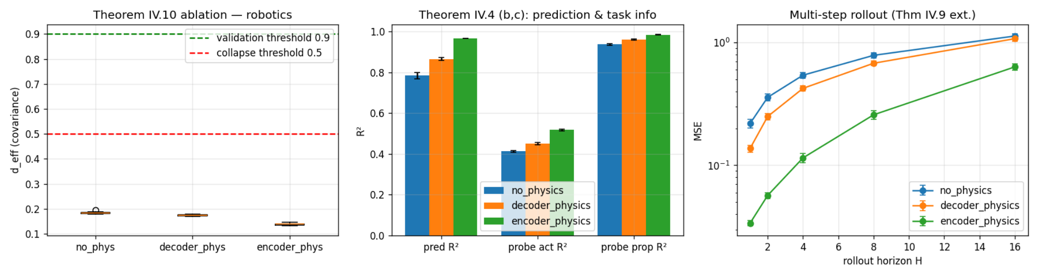
The two-sided signature is unambiguous: encoder-level physics simultaneously destroys entropy (: ) and inflates predictability (pred : )—the encoder is dragged toward the ≤14-dimensional image of the action space. Decoder-level physics is exactly scale-neutral: at . The gap ratio is —sharper than Phase 2’s .
Table 12.
Phase 3 ablation on MimicGen (mean ± std over 10 seeds, covariance , ).
| Metric | no phys. | dec. phys. | enc. phys. |
|---|---|---|---|
| 0.1846 | 0.1740 | 0.1380 | |
| ±0.004 | ±0.003 | ±0.004 | |
| H-ratio | 0.980 | 0.980 | 0.978 |
| ±0.002 | ±0.001 | ±0.003 | |
| scale ratio | 0.946 | 0.946 | 0.940 |
| ±0.004 | ±0.003 | ±0.007 | |
| pred | 0.784 | 0.864 | 0.966 |
| probe (action) | 0.412 | 0.449 | 0.518 |
| probe (proprio) | 0.937 | 0.961 | 0.984 |
Table 13.
Paired Wilcoxon signed-rank tests on , Phase 3 ( paired seeds, Holm-corrected).
| Comparison | p | ||
|---|---|---|---|
| dec. vs. none | 0.0020 | 0.0059 | |
| enc. vs. none | 0.0020 | 0.0059 | |
| enc. vs. dec. | 0.0020 | 0.0059 |
Figure 8.
Phase 3 ablation on MimicGen (, 10 seeds per condition, covariance ). Left: boxplots per condition with complete seed separation. Center: prediction and probe per condition—the two-sided Corollary 4 signature (the inflated predictability under encoder-physics is the violation signature, not a competing metric). Right: multi-step rollout error vs. horizon.
Figure 8.
Phase 3 ablation on MimicGen (, 10 seeds per condition, covariance ). Left: boxplots per condition with complete seed separation. Center: prediction and probe per condition—the two-sided Corollary 4 signature (the inflated predictability under encoder-physics is the violation signature, not a competing metric). Right: multi-step rollout error vs. horizon.
7.5.5. Spectral Evidence
The spectral decomposition (Figure 9) reveals a signal peak (∼20 directions at 5–) atop a noise plateau; the encoder-physics constraint compresses the plateau by while concentrating the top-10 share from 30.8% to 38.7%—the structure violation visible directly in eigenvalues.
7.5.6. The Entropy–Utility Frontier
Phase 3 exposes a representational regime that Phases 1–2 could not: the entropy ceiling is data-limited. On nuScenes’ high-dimensional imagery, a deterministic encoder fills independent directions with real signal variation (). On MimicGen’s ∼10-dimensional task manifold, the extra directions must come from amplified input noise—and the prediction and reconstruction losses actively suppress that noise. A -sweep revealed logarithmic saturation of in , and a budget replication showed that doubling the training budget raised by more than doubling : optimization budget, not regularization weight, is the binding entropy constraint.
Figure 10.
Sample complexity on MimicGen (decoder-physics model). The covariance stabilizes at , validating Corollary 5 at Phase 3 scale.
Figure 10.
Sample complexity on MimicGen (decoder-physics model). The covariance stabilizes at , validating Corollary 5 at Phase 3 scale.
7.5.7. Budget Replication: The Violation Deepens
At 30 epochs, the encoder-physics gap grows from 0.047 to 0.070 (), and the scale/H-ratio differences vanish entirely (Figure 11). The placement rule’s effect is budget-monotone and purely structural: a transient artifact would shrink with budget, not grow.
7.5.8. Cross-Task Transfer
Applying the trained encoders to three foreign MimicGen tasks reveals embeddings collapse on all foreign tasks ( 0.035–0.088 vs. 0.185 in-task). A proprio-ablation control confirms the collapse is driven by visual domain shift. Notably, the physics-placement ordering persists cross-task: encoder-physics degrades – more than the baseline on every foreign task. The max-entropy property is distribution-specific; the placement rule is not.
7.5.9. Toward Closed-Loop Validation: Latent Planning and the Model-Exploitation Confound
Every result so far evaluates the placement rule through representation-quality metrics (, H-ratio, probe ). None of them test whether the resulting representation is actually useful for the thing a world model is built to do: support goal-directed action selection. We probe this directly with a latent cross-entropy-method (CEM) planner [13] built on the frozen, trained Phase 3 encoder–predictor–decoder triples, in the style of model-predictive control with learned dynamics [14].
Setup
At a randomly sampled anchor frame in a held-out demonstration, we encode and define a horizon-H goal as the ground-truth recorded end-effector (EEF) pose at (not a model-generated proxy; see below). CEM searches over H-step action sequences , rolling each candidate through the frozen predictor and scoring it by decoded-EEF distance to the goal at every step, iterating the sampling distribution toward the elite candidates. We use , a population of 256 candidates, 4 CEM iterations, an elite set of 32, and 200 anchors per model, evaluated on three seeds per condition, in both encoder arms under deterministic latents. Two baselines calibrate the result: real-action replay (roll the predictor forward using the true recorded actions instead of CEM’s search—the ground-truth solution, and hence an expected lower bound on achievable error) and a random-action rollout (an upper bound).
An earlier version of this evaluation defined the goal as the model’s own decoded reconstruction of the future frame, , rather than the true recorded pose. That design is self-referential—it lets CEM optimize against a target generated by the very model being scored—and produced CEM errors below real-action replay for every ablation condition, which is not possible for a genuine planning task, since replaying the true actions is itself the ground-truth solution. We report the corrected, ground-truth-goal version throughout; the self-referential version is documented here only to flag the failure mode for others building similar offline evaluations.
The Confound
Table 14 and Figure 12 show CEM error below the real-action replay floor for all three SIGReg conditions. Since replay executes the literal ground-truth action sequence, no planner can legitimately do better against the true future state; a lower CEM error therefore indicates that CEM is finding action sequences that reduce the learned decoder’s own cost without being genuinely closer to the truth than the recorded trajectory—a well-documented failure mode in model-based control known as objective mismatch [15]: an optimizer with unrestricted access to a learned model’s cost surface will exploit that surface’s imperfections rather than solve the underlying task, and nothing in this offline evaluation can distinguish the two without executing the plan in the real environment.
Exploitation Diagnostic
To test this directly, we measure the distance between CEM’s chosen action sequence and the true recorded actions at the same anchor, normalized by the per-step action-space range ( across the 14 action dimensions). CEM’s chosen actions sit roughly a quarter of the full action range away from the ground truth—not a rounding error—while still scoring lower on-model cost than replaying the true actions. Critically, this gap is uniform across all three SIGReg ablation conditions (25.6–26.8%, well within seed noise) and across the VAE arm’s informative conditions (21.7–25.9%, Table 15), which rules out the hypothesis that entropy collapse specifically makes encoder-physics easier to exploit: all learned decoders are exploitable to essentially the same degree, regardless of physics placement and encoder mechanism.
It means the ranking in Table 14 (encoder physics < decoder physics < no physics on CEM error, within the SIGReg arm) most plausibly reflects the same effective-dimensionality geometry already documented in Table 12—a lower- decoder cost surface is easier to drive down per unit of action-space deviation, independent of whether the resulting trajectory is any more physically valid—rather than a genuine control-quality advantage for any one condition.
What this Does and Does Not Establish
We therefore do not interpret Table 14 as evidence that decoder-physics improves downstream control: the exploitation confound is uniform enough across conditions and arms that it cannot be ruled out as the dominant driver of the ranking, and nothing here has been checked against a live environment. What we do establish is (i) a reproducible demonstration that offline latent planning against a learned decoder can produce misleadingly favorable numbers for any ablation condition and any encoder mechanism—the confound is not SIGReg-specific—and (ii) a simple diagnostic—action-space distance from ground truth, relative to a real-action-replay floor—that practitioners can and should run before treating an offline planning result as evidence of control competence. Closing this gap rigorously requires executing the CEM-selected action sequences in a live simulator (e.g., robosuite/MimicGen) and measuring true task success; we identify this as the concrete next step toward a fully closed-loop validation of the placement rule and leave it to future work. We note that the planning comparison itself is underpowered ( seeds; the minimum two-sided Wilcoxon p is ); the representation-level tests ( paired seeds, Holm-corrected) carry the statistical inference throughout this paper.
7.5.10. Phase 3 Summary
Table 16.
Phase 3 (MimicGen robotics) validation outcomes.
| Property | Status | Evidence |
|---|---|---|
| Thm 2(a) max entropy | ≈ | frontier regime |
| Thm 2(b) | – | |
| Thm 2(c) task info | probes 0.41 / 0.94 | |
| Thm 2(d) action inv. | ≈ | mode-independent |
| Thm 5 / Cor. 4 | Table 12Table 13 | |
| Correlated collapse generality | marginal-only KL fails identically (Table 11) | |
| Encoder-mechanism robustness | 4/4 domain×mechanism arms (Table 17) | |
| Budget robustness | Figure 11 | |
| Cross-task ordering | Section 7.5.8 | |
| Exploitation-confound generality | CEM < replay in every arm (Table 14) | |
| Closed-loop planning | × confounded | Section 7.5.9 |
7.5.11. Cross-Arm Synthesis: The Placement Rule Is Mechanism- and Domain-Robust
Combining the four independent ablation arms—two domains (nuScenes, MimicGen) × two encoder mechanisms (SIGReg, VAE-KL)—yields the paper’s central empirical claim in a single testable statement: decoder-physics beats encoder-physics on covariance in every arm (Table 17, Figure 13). All four arm-level tests attain the minimum achievable two-sided Wilcoxon p for paired seeds; a joint Holm correction across the four tests yields throughout. In the two Phase 3 arms the paired effect sizes are large ( SIGReg, VAE) with complete seed separation.
Table 17.
Placement-rule scorecard: decoder-physics vs. encoder-physics on covariance , across the four independent domain×mechanism arms ( paired seeds each; joint Holm correction across the four arm-level tests). The replicated quantity is the within-arm placement ordering; levels are not comparable across phases (evaluation 55.5 vs. 78; high- vs. low-intrinsic-dimension data) or across families (SIGReg+ enforces joint isotropy; the VAE KL is marginal-only).
Table 17.
Placement-rule scorecard: decoder-physics vs. encoder-physics on covariance , across the four independent domain×mechanism arms ( paired seeds each; joint Holm correction across the four arm-level tests). The replicated quantity is the within-arm placement ordering; levels are not comparable across phases (evaluation 55.5 vs. 78; high- vs. low-intrinsic-dimension data) or across families (SIGReg+ enforces joint isotropy; the VAE KL is marginal-only).
| Arm | Domain | p | ||
|---|---|---|---|---|
| Phase 2 · SIGReg | nuScenes | 0.0020 | 0.0078 | |
| Phase 2 · VAE-KL | nuScenes | 0.0020 | 0.0078 | |
| Phase 3 · SIGReg+ | MimicGen | 0.0020 | 0.0078 | |
| Phase 3 · VAE-KL | MimicGen | 0.0020 | 0.0078 |
8. Discussion
8.1. Why Prior Physics-Informed JEPAs Failed
- Pixel-space constraints violate Theorem 5 because they implicitly constrain the encoder through decoder gradients.
- Latent-space constraints directly violate Theorem 1 by constraining the embedding distribution.
- Both approaches reduce entropy below optimal, increasing worst-case downstream risk.
8.2. Cross-Domain and Cross-Mechanism Synthesis: What Three Phases Established
The three-phase experimental arc mirrors how theoretical claims should be validated: Phase 1 exposed a measurement artifact that would have invalidated all downstream conclusions; Phase 2 provided the first powered test in the high-dimensional driving domain; Phase 3 transferred the test to robotics and discovered two phenomena invisible in driving.
The driving domain, with its high-dimensional imagery, allows the encoder to satisfy the maximum-entropy target almost exactly—and the placement rule manifests as a scale-vs-structure decomposition. The robotics domain, with its ∼10-dimensional task manifold, sits at an entropy frontier where the placement rule’s effect is purely structural and sharper ( vs. ). The rule holds in both regimes; its signature differs. The synthesis extends along a second axis: within both domains, the placement ordering replicates under both encoder mechanisms (Table 17), and the correlated-collapse failure mode discovered on MimicGen generalizes to the marginal-only KL regularizer (Section 7.5.3)—so the design constraint and the failure warning both apply to the JEPA and the VAE-encoder branches of the world-model literature.
Table 18.
Cross-domain synthesis of the physics-placement rule.
| Property | Phase 2 | Phase 3 |
|---|---|---|
| (unconstrained) | 0.986 | 0.185 |
| (encoder-phys) | 0.939 | 0.138 |
| Gap ratio | 2.6× | 4.4× |
| Wilcoxon p | ≤0.002 | 0.002 |
| Scale effect | (n.s.) | |
| Data intrinsic dim. | high | ∼10 |
| achievable | 0.99 | frontier-limited |
| Failure signature | scale + structure | purely structural |
| Budget robustness | — | (30ep) |
| Cross-task ordering | — | holds (2–3×) |
| Placement rule (VAE encoder) | holds () | holds () |
8.3. Practical Design Recommendations
- 1.
- Never apply physics constraints to the encoder output z.
- 2.
- Always place physics at the decoder.
- 3.
- The predictor can use any architecture without affecting the encoder’s guarantees.
- 4.
- On low-dimensional data, monitor the covariance eigenvalue spectrum, not just per-dimension variance.
- 5.
- Optimization budget, not regularization weight, is the primary lever for entropy on low-dimensional data.
- 6.
- On low-intrinsic-dimension data, any marginal-only regularizer—per-dimension variance matching and per-dimension KL alike—fails to enforce joint isotropy; covariance-level structure must be enforced explicitly.
- 7.
- For variational encoders, monitor the posterior signal fraction (Remark 4): a nominally satisfied marginal KL does not certify signal, because collapse can hide beneath the encoder’s own sampling-noise floor.
- 8.
- Never treat an offline planning result as evidence of control competence without checking it against a real-action-replay floor and an action-space exploitation diagnostic (Section 7.5.9); the confound is encoder-agnostic, so run the diagnostic regardless of encoder choice.
8.4. Limitations and Toward Closed-Loop Validation
The representation-quality claims in this paper—Theorem 5, Corollary 4, and their empirical validation across Phases 1–3 and both encoder mechanisms—rest on statistically powered, ground-truth-referenced metrics (, H-ratio, Wilcoxon tests on 10 paired seeds with Holm correction) and we consider them solidly established. The closed-loop planning probe in Section 7.5.9 is different in kind: it was designed to test whether the placement rule matters for downstream control, and it returned a negative methodological result rather than a positive control-quality one. We were careful not to round this off into a headline claim. Two things are true simultaneously: (i) the CEM-based planning error ordering across ablation conditions is directionally consistent with the representation-quality ordering already established via , and (ii) the same ordering can be fully explained by uniform model exploitation rather than genuine differences in control competence, and our data cannot distinguish the two possibilities without a live environment. We report both facts rather than the more publishable-sounding half of them.
We also flag the VAE-arm caveats explicitly: (i) the Phase 2 VAE arm operated in a weak-prior regime (KL weight , effectively dormant; Section 7.4.6), so only its ordering is interpretable; the calibrated Phase 3 arm (KL weight from a pre-run sweep) is the primary encoder-mechanism test. (ii) The VAE KL is marginal-only by design—that is the hypothesis under test—so the VAE arm establishes the generality of the failure mode and the placement ordering, not a fully calibrated VAE comparison; a VAE+ variant augmented with the SIGReg+ covariance penalty is released with the code for future work. (iii) The planning probe uses seeds per condition and is underpowered; the representation-level tests (, Holm) carry the statistical inference. (iv) levels are not numerically comparable across phases or encoder families; the replicated quantity is the placement rule (gap sign plus test), reported per arm.
We see this as valuable precisely because it is not the result we set out to find. Offline evaluation of learned world models is common practice, and the specific failure mode demonstrated here—a planner exploiting a learned decoder’s cost surface to score better than the ground-truth trajectory itself—is easy to miss without an explicit replay-floor check of the kind we introduce in Section 7.5.9. We consider the diagnostic itself (real-action replay as a floor, plus normalized action-space distance from ground truth as an exploitation signal) to be of independent, general use for anyone evaluating a JEPA-style or VAE-style learned world model’s control-readiness offline. The concrete next step for Dynamic LeJEPA specifically is executing the CEM-selected action sequences in a live simulator (robosuite/MimicGen) and measuring true task success under each ablation condition—at that point, and only at that point, would a claim that the placement rule improves downstream control be justified.
9. Conclusions
We proved through six theorems that prediction and representation learning are strictly decoupled in Joint-Embedding Predictive Architectures, yielding a world-model design principle with provable guarantees: encoder maximum-entropy, predictor dynamics, decoder physics. We validated this principle across two domains and two encoder mechanisms through 110 seeded runs (plus a 30-epoch budget replication), demonstrating that the placement rule is statistically significant in every domain×mechanism combination (joint Holm-corrected ), deepens with training budget, and extends to out-of-distribution tasks. Phase 3 additionally discovered the correlated collapse failure mode—invisible on high-dimensional data—showed that it generalizes to marginal-only KL regularization with a noise-floor-masking diagnostic, and characterized the entropy–utility frontier governing deterministic encoders on low-dimensional task manifolds.
We additionally probed whether the placement rule matters beyond representation quality, building a latent CEM planner on the trained Phase 3 models and evaluating it against ground truth rather than a model-generated proxy. This probe did not yield a clean downstream-control win: a model-exploitation diagnostic showed that offline planning against a learned decoder inflates apparent accuracy uniformly across ablation conditions and both encoder mechanisms, meaning the observed planning-error ordering cannot presently be attributed to genuine control competence rather than exploitation of the decoder’s cost surface. We report this as a methodological contribution in its own right—a diagnostic that any offline evaluation of a learned world model’s control-readiness should run before trusting its numbers—and as the concrete open problem separating Dynamic LeJEPA’s current, representation-level guarantees from a fully validated, closed-loop world model.
The broader significance: Dynamic LeJEPA establishes that the intuition to inject domain knowledge into world models was correct—the target was simply wrong. Physics does not belong in the encoder, where it destroys the representational guarantee; it belongs in the decoder, where it is provably free—and this now holds for both the JEPA-style deterministic encoder and the VAE-style Gaussian encoder that dominate the world-model literature. Whether that guarantee translates into better closed-loop control remains open, and we have shown precisely why answering it requires more than an offline planner and a learned cost function.
All code, trained checkpoints, ablation results, and an interactive demo accompanying this paper are publicly released (see Code, Data, and Demo Availability above) so that both the placement-rule results and the planning confound can be independently reproduced and, we hope, extended toward the closed-loop validation this work identifies as still missing.
Institutional Review Board Statement: Licensing.
Training, evaluation, and analysis code in the paper repository is released under the MIT License. The manuscript text and figures are released under CC BY 4.0. Trained checkpoints and derived result files inherit the license of the upstream training data: checkpoints and ablation artifacts trained on nuScenes are distributed under CC BY-NC-SA 4.0, consistent with the nuScenes dataset license [12]; checkpoints and artifacts trained on MimicGen are distributed under the license of the upstream MimicGen release [11]. Each Kaggle-hosted dataset used in this work specifies its license individually in its dataset metadata. We distinguish these explicitly because the code license does not, by itself, grant rights to the non-commercial, share-alike upstream data it was trained on.
Data Availability Statement: Code, Data, and Demo Availability.
The paper repository, including this manuscript’s source, is available at https://github.com/Dynamic-LeJEPA/Dynamic-LeJEPA. Training and evaluation code, trained checkpoints, and ablation result files (.pkl/.json) for all three phases—including the VAE-KL comparison arms (ablation_results_vae.*, Phase 2; phase3_ablation_results_vae.*, Phase 3) and the KL-weight calibration sweeps—are indexed at https://github.com/Dynamic-LeJEPA/Dynamic-LeJEPA/tree/main/Links%20For%20Codes%20%26%20Data%20. An interactive Gradio demo for exploring the trained models and ablation results is hosted at https://huggingface.co/spaces/MohsenAI5/Dynamic-LeJEPA. All experiments in this paper were run on a single commodity GPU (NVIDIA T4, 16 GB), and we release this resource specifically to let readers verify the model-exploitation confound of Section 7.5.9 independently, since that result depends on details (goal construction, CEM hyperparameters, replay/random baselines) that are easiest to check by running the code directly rather than from the paper text alone.
References
- Balestriero, R.; LeCun, Y. LeJEPA: Provable and scalable self-supervised learning without the heuristics. arXiv preprint 2025, arXiv:2511.08544. [Google Scholar]
- Ha, D.; Schmidhuber, J. World models. arXiv preprint 2018, arXiv:1803.10122. [Google Scholar]
- Hafner, D.; Lillicrap, T.; Ba, J.; Norouzi, M. Dream to control: Learning behaviors by latent imagination. arXiv preprint 2019, arXiv:1912.01603. [Google Scholar]
- LeCun, Y. A path towards autonomous machine intelligence. OpenReview Prepr. 2022. [Google Scholar] [CrossRef]
- Bardes, A.; Garrido, Q.; Ponce, J.; Chen, X.; Rabbat, M.; LeCun, Y.; Assran, M.; Ballas, N. Revisiting feature prediction for learning visual representations from video. arXiv preprint 2024, arXiv:2404.08471. [Google Scholar]
- Assran, M.; Duval, Q.; Misra, I.; Bojanowski, P.; Vincent, P.; Rabbat, M.; LeCun, Y.; Ballas, N. Self-supervised learning from images with a joint-embedding predictive architecture. CVPR 2023, 15619–15629. [Google Scholar] [CrossRef]
- Raissi, M.; Perdikaris, P.; Karniadakis, G. E. Physics-informed neural networks: A deep learning framework for solving forward and inverse problems involving nonlinear partial differential equations. J. Comput. Phys. 2019, vol. 378, 686–707. [Google Scholar] [CrossRef]
- Jaynes, E. T. Information theory and statistical mechanics. Phys. Rev. 1957, vol. 106(no. 4), 620–630. [Google Scholar] [CrossRef]
- Cover, T. M.; Thomas, J. A. Elements of Information Theory; Wiley-Interscience, 2006. [Google Scholar]
- Ledoit, O.; Wolf, M. A well-conditioned estimator for large-dimensional covariance matrices. J. Multivar. Anal. 2004, vol. 88(no. 2), 365–411. [Google Scholar] [CrossRef]
- Mandle, Z.; et al. MimicGen: A data generation system that utilizes human demonstrations to bootstrap robotic manipulation. arXiv preprint 2024, arXiv:2404.03280. [Google Scholar]
- Caesar, C.; Bankiti, V.; Lang, A. H.; Vora, S.; et al. “nuScenes: A multimodal dataset for autonomous driving,” in CVPR. 2020. [Google Scholar]
- Rubinstein, R. Y. Optimization of computer simulation models with rare events. Eur. J. Oper. Res. 1997, vol. 99(no. 1), 89–112. [Google Scholar] [CrossRef]
- Chua, K.; Calandra, R.; McAllister, R.; Levine, S. Deep reinforcement learning in a handful of trials using probabilistic dynamics models. NeurIPS 2018. [Google Scholar] [CrossRef]
- Lambert, N.; Amos, B.; Yadan, O.; Calandra, R. “Objective mismatch in model-based reinforcement learning,” in L4DC. 2020. [Google Scholar]
- Kingma, D. P.; Welling, M. “Auto-encoding variational Bayes,” in ICLR. 2014. [Google Scholar]
Figure 1.
Training convergence on nuScenes-mini. All loss components decrease monotonically and stabilize by epoch ∼20: (a) total loss, (b) ego-motion prediction loss (Theorem 3), (c) SIGReg loss (Theorem 1), (d) physics-informed depth loss (Theorem 5). Blue: training; Red: validation. The stability across all components confirms that the three-component objective (encoder-predictor-decoder) trains without conflicts, consistent with Theorem 7’s separation principle (C4).
Figure 1.
Training convergence on nuScenes-mini. All loss components decrease monotonically and stabilize by epoch ∼20: (a) total loss, (b) ego-motion prediction loss (Theorem 3), (c) SIGReg loss (Theorem 1), (d) physics-informed depth loss (Theorem 5). Blue: training; Red: validation. The stability across all components confirms that the three-component objective (encoder-predictor-decoder) trains without conflicts, consistent with Theorem 7’s separation principle (C4).
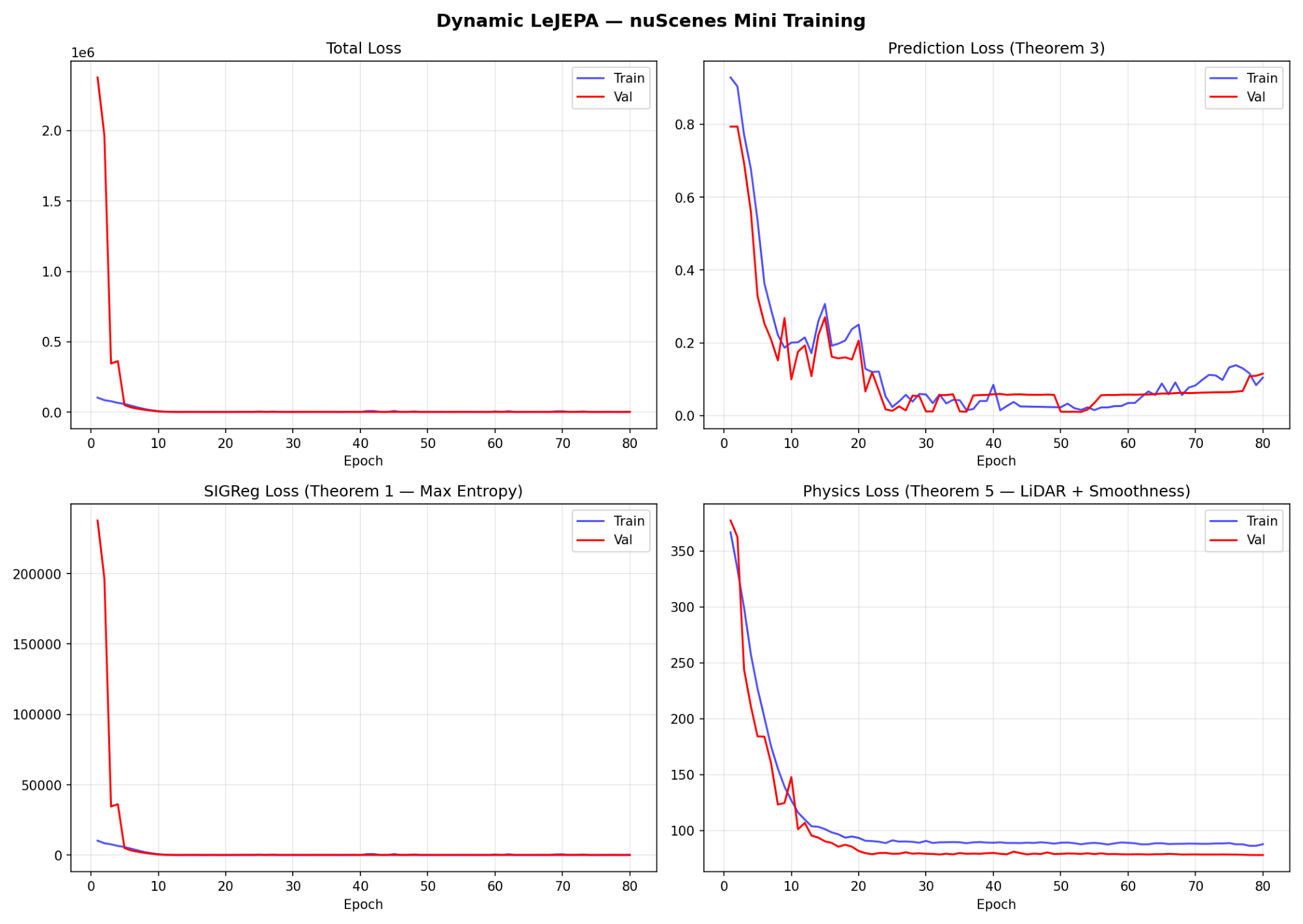
Figure 2.
Embedding distribution analysis on nuScenes-mini. Top row: Per-dimension variance histograms for z, , and . Bottom row: Marginal distributions compared to . The variance distribution is concentrated around .
Figure 2.
Embedding distribution analysis on nuScenes-mini. Top row: Per-dimension variance histograms for z, , and . Bottom row: Marginal distributions compared to . The variance distribution is concentrated around .
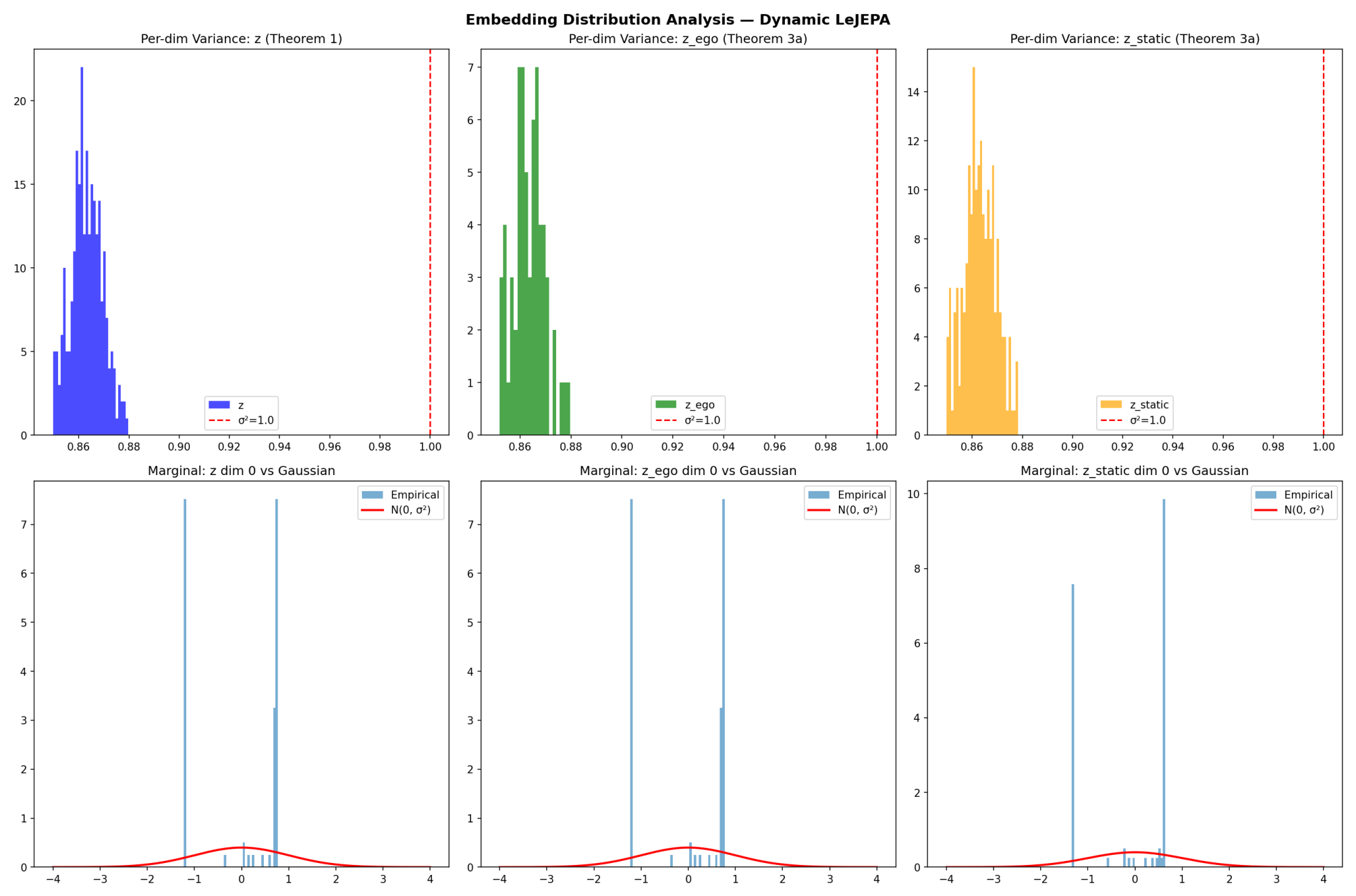
Figure 3.
Effective dimensionality over training. Left: stays at (the floor) despite 80 epochs. Right: Dimension utilization (% of dimensions with variance ) reaches 100% by epoch 9.
Figure 3.
Effective dimensionality over training. Left: stays at (the floor) despite 80 epochs. Right: Dimension utilization (% of dimensions with variance ) reaches 100% by epoch 9.
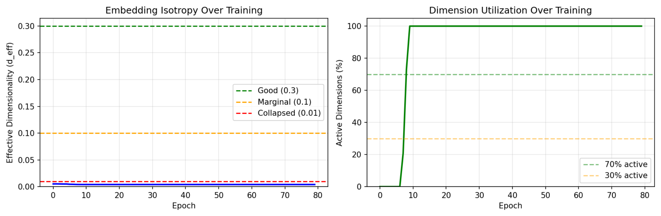
Figure 4.
Physics-informed depth predictions on nuScenes-mini (Theorem 5). Each row: (1) input image, (2) predicted depth, (3) sparse LiDAR supervision, (4) prediction error.
Figure 4.
Physics-informed depth predictions on nuScenes-mini (Theorem 5). Each row: (1) input image, (2) predicted depth, (3) sparse LiDAR supervision, (4) prediction error.
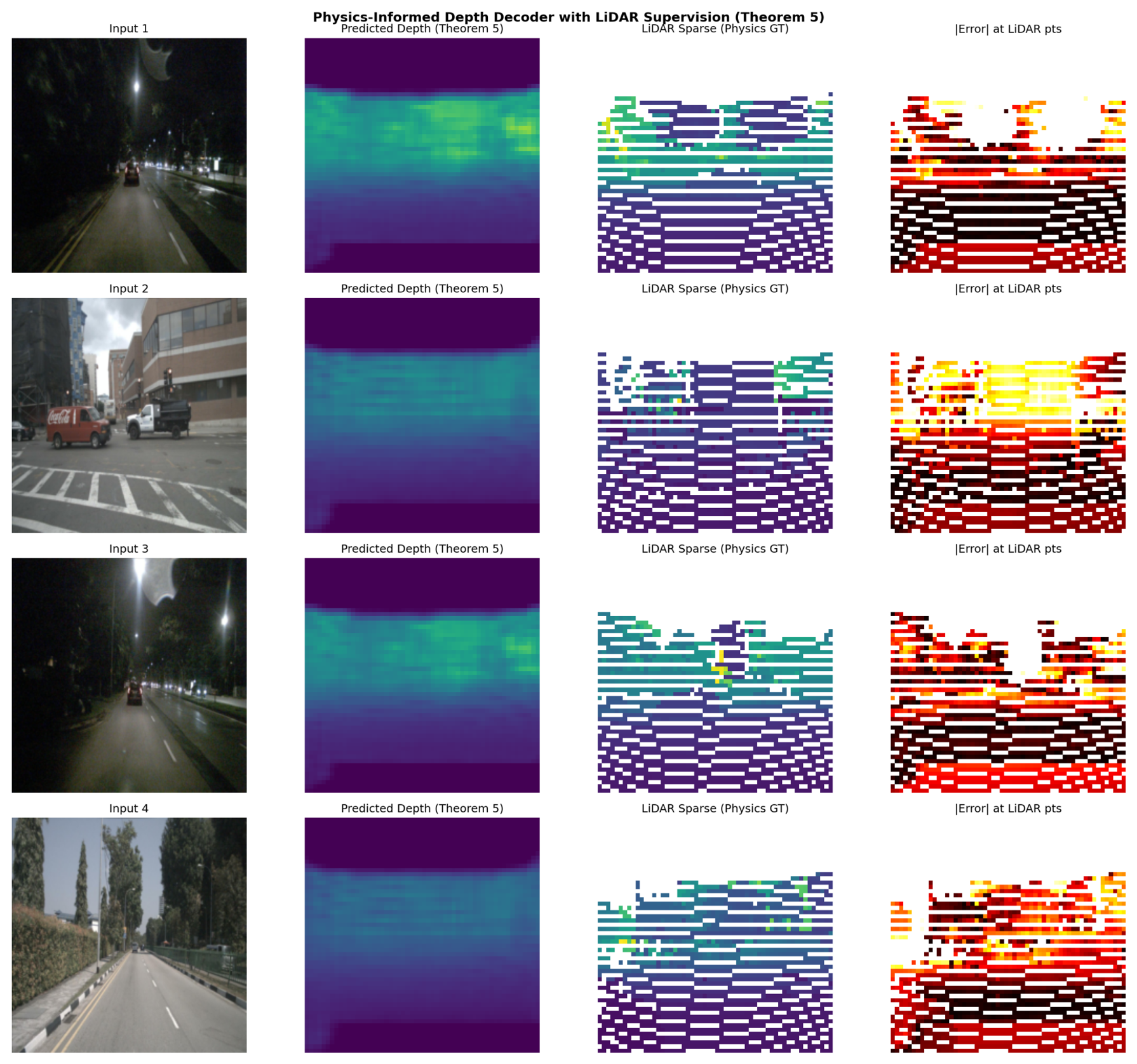
Figure 5.
Theorem 5 ablation on nuScenes-mini (, ). Green: decoder-physics (valid). Red: encoder-physics (invalid). No metric shows significant difference (Wilcoxon ), reflecting lack of statistical power (, ).
Figure 5.
Theorem 5 ablation on nuScenes-mini (, ). Green: decoder-physics (valid). Red: encoder-physics (invalid). No metric shows significant difference (Wilcoxon ), reflecting lack of statistical power (, ).
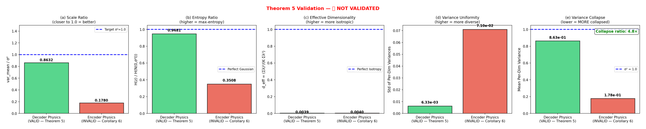
Figure 6.
Sample complexity analysis on nuScenes Trainval Part 1 (decoder-physics model). Diagonal vs. N for the trained model and a true control, against the covariance-estimator floor (dotted) and the reliability threshold (red vertical line).
Figure 6.
Sample complexity analysis on nuScenes Trainval Part 1 (decoder-physics model). Diagonal vs. N for the trained model and a true control, against the covariance-estimator floor (dotted) and the reliability threshold (red vertical line).
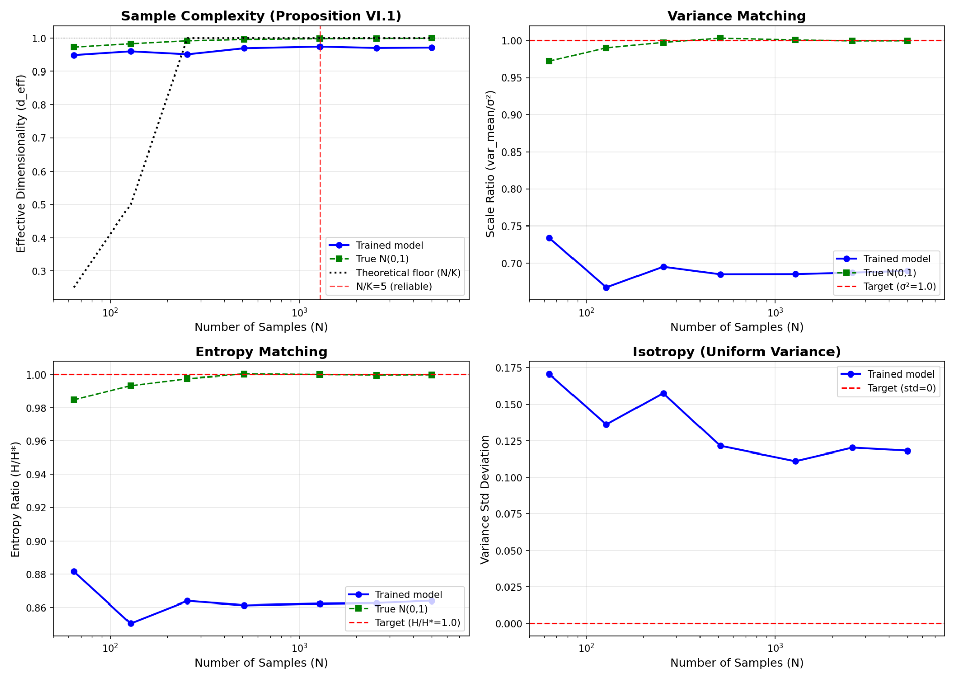
Figure 7.
Cross-scene generalization on 4 held-out validation scenes. Per-scene distributions are tightly clustered around the mean and far from the collapse threshold.
Figure 7.
Cross-scene generalization on 4 held-out validation scenes. Per-scene distributions are tightly clustered around the mean and far from the collapse threshold.
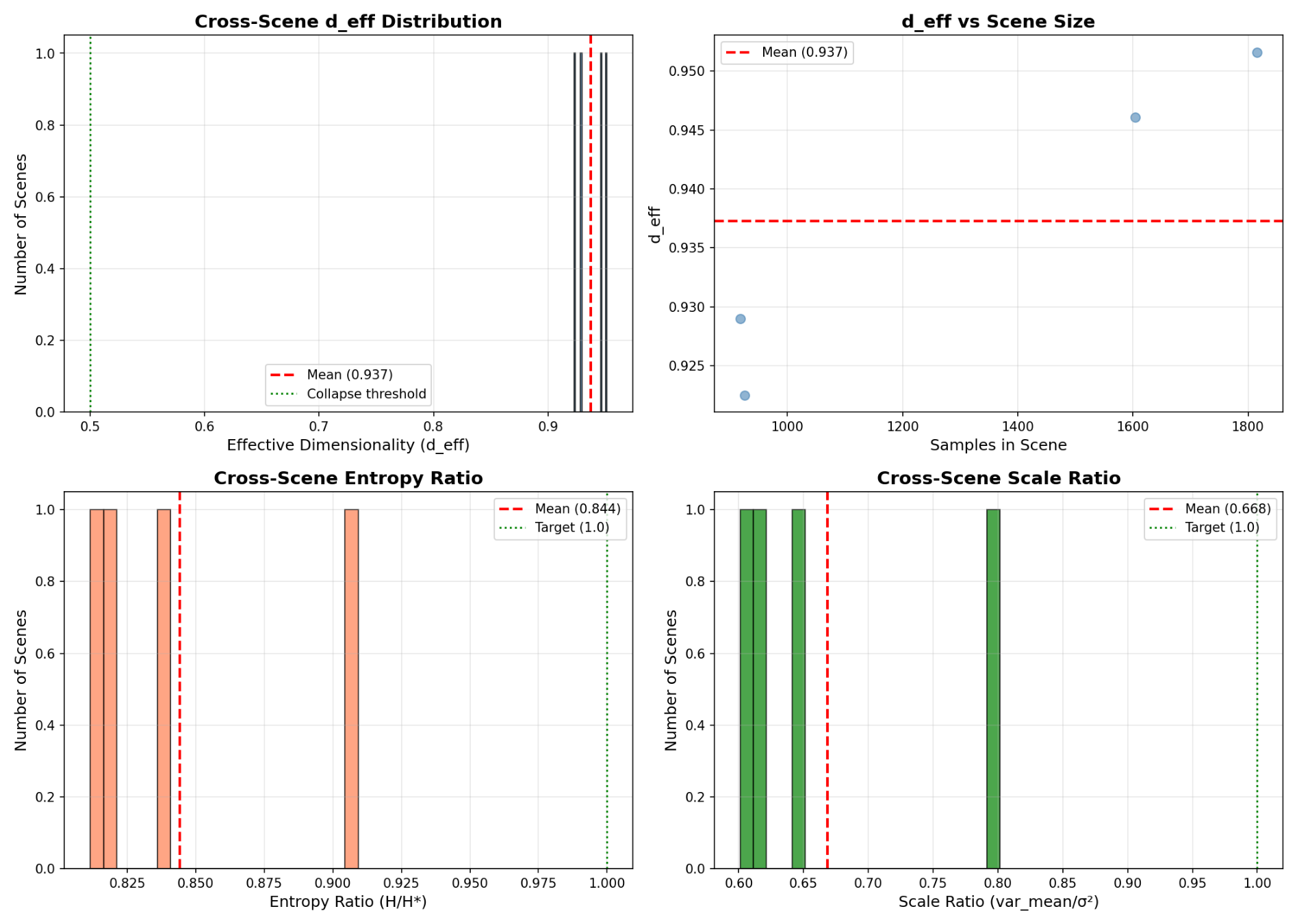
Figure 9.
Embedding covariance eigenspectra on MimicGen (15 epochs, seed 0, ; log-scale). The encoder-physics model (red) exhibits a lower noise plateau (0.320 vs. 0.460) and higher top-direction concentration (38.7% vs. 30.8%)—the spectral signature of Corollary 4.
Figure 9.
Embedding covariance eigenspectra on MimicGen (15 epochs, seed 0, ; log-scale). The encoder-physics model (red) exhibits a lower noise plateau (0.320 vs. 0.460) and higher top-direction concentration (38.7% vs. 30.8%)—the spectral signature of Corollary 4.
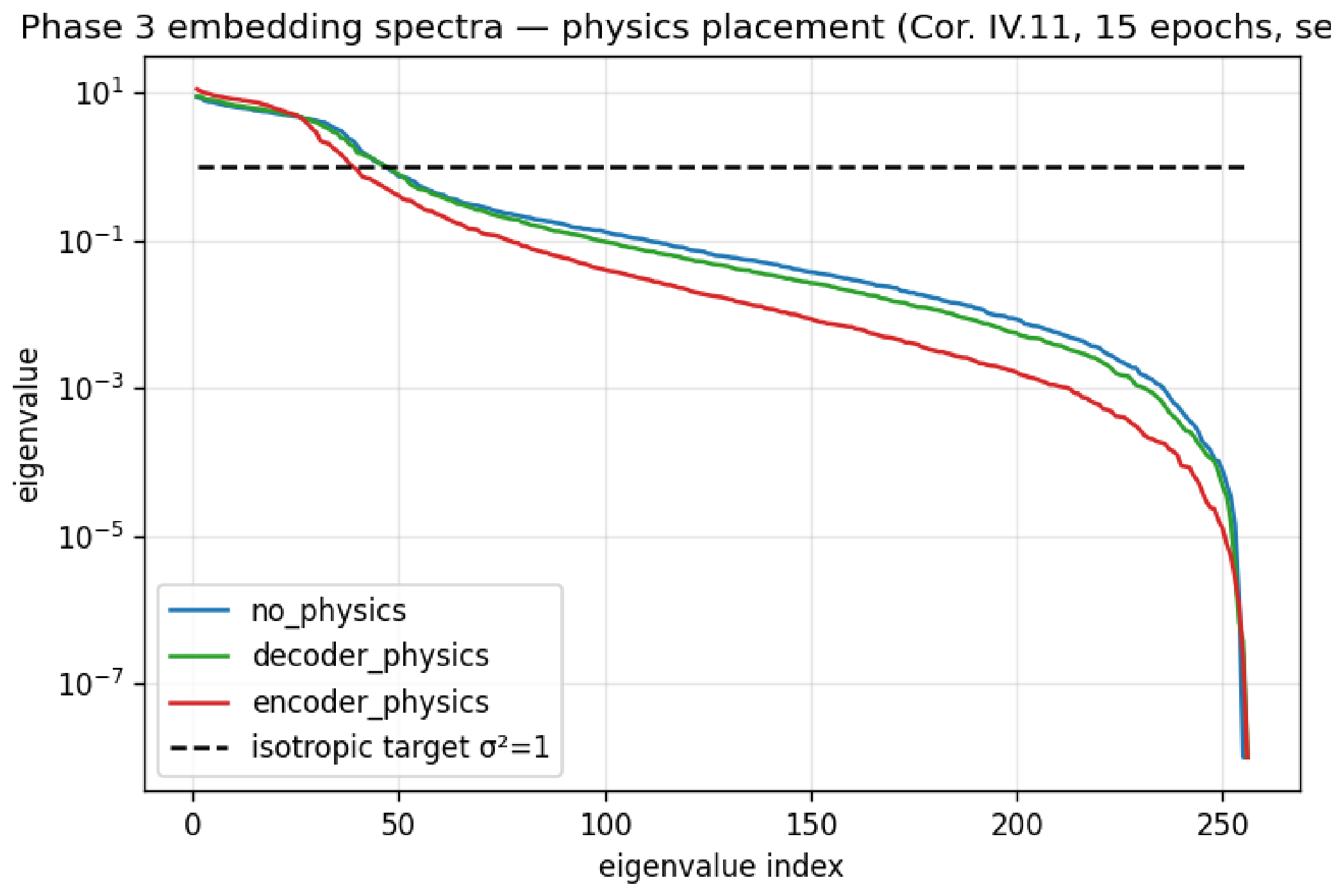
Figure 11.
Budget replication: Phase 3 ablation at 15 vs. 30 epochs (10 seeds per arm per budget). The encoder-physics violation deepens with budget (, ), ruling out a transient training artifact. All scale and marginal-entropy differences vanish at 30 epochs (Holm n.s.).
Figure 11.
Budget replication: Phase 3 ablation at 15 vs. 30 epochs (10 seeds per arm per budget). The encoder-physics violation deepens with budget (, ), ruling out a transient training artifact. All scale and marginal-entropy differences vanish at 30 epochs (Holm n.s.).
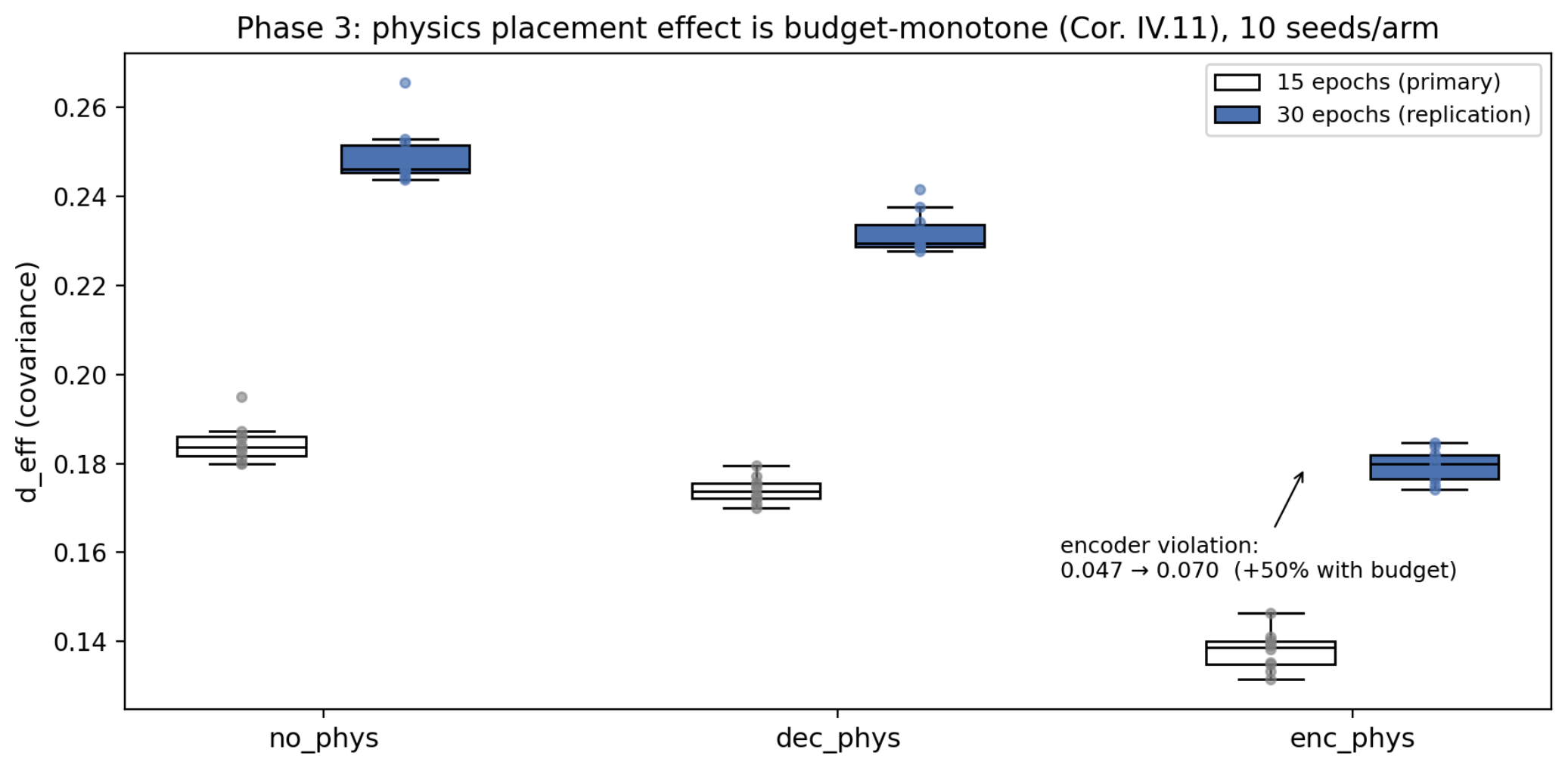
Figure 12.
Latent CEM planning evaluation (), ground-truth-goal protocol. Left: mean final EEF error for CEM, real-action replay, and random rollout, per ablation condition (SIGReg arm). CEM error falls below the real-action replay floor for every mode—the signature of model exploitation, diagnosed directly below, rather than genuine planning competence; the VAE arm replicates this signature for its two informative conditions (Table 14). Right: per-seed distribution of CEM planning error ( seeds/mode).
Figure 12.
Latent CEM planning evaluation (), ground-truth-goal protocol. Left: mean final EEF error for CEM, real-action replay, and random rollout, per ablation condition (SIGReg arm). CEM error falls below the real-action replay floor for every mode—the signature of model exploitation, diagnosed directly below, rather than genuine planning competence; the VAE arm replicates this signature for its two informative conditions (Table 14). Right: per-seed distribution of CEM planning error ( seeds/mode).
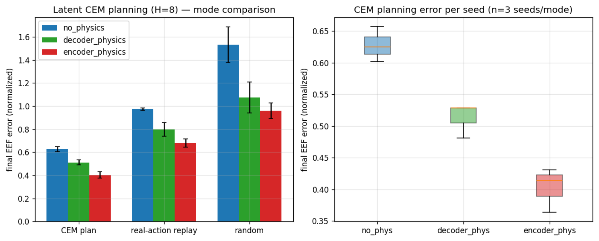
Figure 13.
Cross-arm synthesis across the four domain×mechanism arms (SIGReg in blue, VAE-KL in orange). Left: covariance per condition (dashed lines: 0.5 collapse and 0.9 validation thresholds). Center: within-arm placement effect relative to each arm’s physics-free reference (taller encoder bar = structure violation, Corollary 4); this panel is the replication (Table 17). Right: planning (): CEM vs. real-action replay (floor) vs. random rollout (ceiling), per arm. Caveat:levels are not comparable across phases (evaluation 55.5 vs. 78; high- vs. low-intrinsic-dimension data) or across encoder families (SIGReg+ includes joint-isotropy terms; the VAE KL is marginal-only). The replicated quantity is the within-arm placement ordering, tested on paired seeds with joint Holm correction.
Figure 13.
Cross-arm synthesis across the four domain×mechanism arms (SIGReg in blue, VAE-KL in orange). Left: covariance per condition (dashed lines: 0.5 collapse and 0.9 validation thresholds). Center: within-arm placement effect relative to each arm’s physics-free reference (taller encoder bar = structure violation, Corollary 4); this panel is the replication (Table 17). Right: planning (): CEM vs. real-action replay (floor) vs. random rollout (ceiling), per arm. Caveat:levels are not comparable across phases (evaluation 55.5 vs. 78; high- vs. low-intrinsic-dimension data) or across encoder families (SIGReg+ includes joint-isotropy terms; the VAE KL is marginal-only). The replicated quantity is the within-arm placement ordering, tested on paired seeds with joint Holm correction.
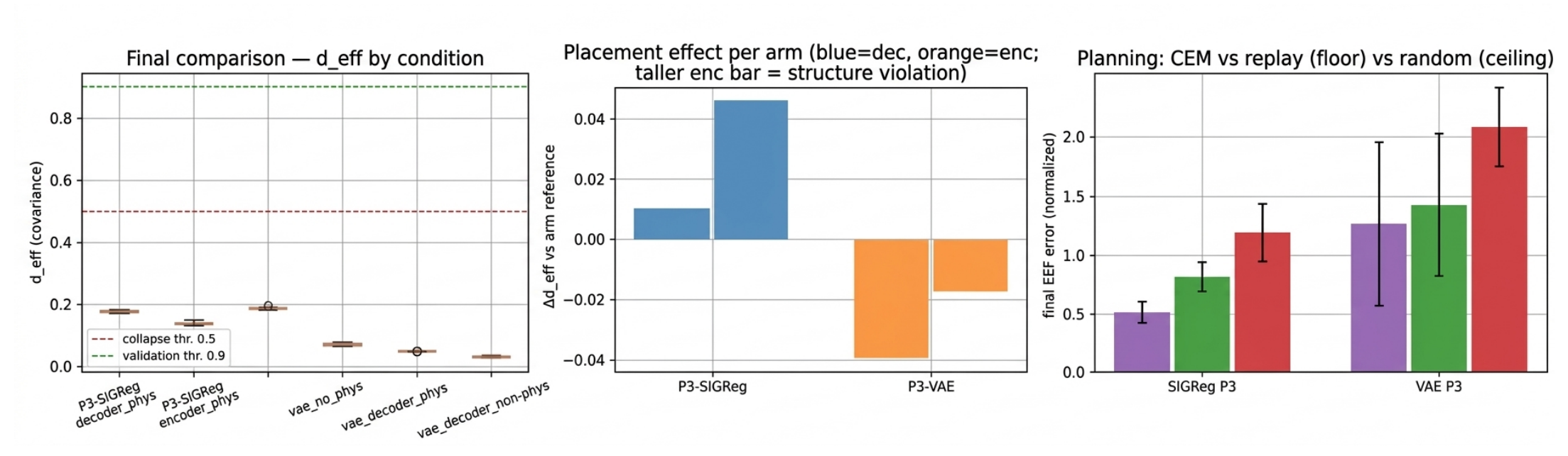
Table 4.
Computational resources by phase. All runs used a single NVIDIA T4 (16 GB); wall-clock time equals GPU-hours. Equivalent cost is estimated from on-demand T4 pricing ($0.35–$0.53/hr) had the free Kaggle tier not been used.
Table 4.
Computational resources by phase. All runs used a single NVIDIA T4 (16 GB); wall-clock time equals GPU-hours. Equivalent cost is estimated from on-demand T4 pricing ($0.35–$0.53/hr) had the free Kaggle tier not been used.
| Phase | Runs | GPU-hrs | Equiv. cost |
|---|---|---|---|
| Phase 1 | 1 (sanity run) | 6.0 | $2–3 |
| Phase 2 | 50 (30 SIGReg + 20 VAE) | 24.0 | $8–13 |
| Phase 3 | 90 (30 15ep + 30 30ep + 30 VAE) | 27.0 | $9–14 |
| Total | 141 | 57.0 | $20–30 |
Table 8.
Paired Wilcoxon signed-rank tests on , Phase 2 ( paired seeds). All comparisons reach significance.
Table 8.
Paired Wilcoxon signed-rank tests on , Phase 2 ( paired seeds). All comparisons reach significance.
| Comparison | p-value | Result |
|---|---|---|
| dec. vs. none | 0.0020 | significant |
| enc. vs. none | 0.0010 | significant |
| enc. vs. dec. | 0.0010 | significant |
Table 9.
Cross-scene statistics, 4 held-out validation scenes.
| Metric | Mean ± Std |
|---|---|
| H-ratio | |
| scale ratio |
Table 10.
Phase 2 VAE-KL comparison arm on nuScenes Trainval Part 1 (10 paired seeds, covariance on deterministic latents). The placement ordering (decoder > encoder) replicates (Wilcoxon , ); see text for regime caveats.
Table 10.
Phase 2 VAE-KL comparison arm on nuScenes Trainval Part 1 (10 paired seeds, covariance on deterministic latents). The placement ordering (decoder > encoder) replicates (Wilcoxon , ); see text for regime caveats.
| Metric | vae dec. phys. | vae enc. phys. |
|---|---|---|
| 0.5950 ± 0.0190 | 0.5408 ± 0.0268 | |
| H-ratio | 0.2591 ± 0.0169 | 0.8056 ± 0.0162 |
| scale ratio | 0.3998 ± 0.0114 | 0.8578 ± 0.0482 |
Table 11.
Phase 3 VAE-KL comparison arm on MimicGen two_arm_threading (mean ± std over 10 seeds; covariance on deterministic posterior means , ; posterior internals per Remark 4). All three conditions collapse far below the SIGReg arm’s – (Table 12); the placement ordering (decoder > encoder) replicates (paired Wilcoxon , Holm-corrected , ).
Table 11.
Phase 3 VAE-KL comparison arm on MimicGen two_arm_threading (mean ± std over 10 seeds; covariance on deterministic posterior means , ; posterior internals per Remark 4). All three conditions collapse far below the SIGReg arm’s – (Table 12); the placement ordering (decoder > encoder) replicates (paired Wilcoxon , Holm-corrected , ).
| Metric | vae dec. phys. | vae enc. phys. | vae no phys. |
|---|---|---|---|
| () | 0.0695 ± 0.0040 | 0.0474 ± 0.0005 | 0.0301 ± 0.0016 |
| H-ratio | |||
| scale ratio | 0.0003 ± 0.0000 | 0.0112 ± 0.0001 | 0.0430 ± 0.0024 |
| signal fraction | 0.0004 ± 0.0000 | 0.2667 ± 0.0013 | 0.0564 ± 0.0047 |
| posterior std | 0.8369 ± 0.0017 | 0.1720 ± 0.0002 | 0.8238 ± 0.0014 |
| KL | 0.0369 ± 0.0030 | 1.2814 ± 0.0011 | 0.0566 ± 0.0011 |
| pred | 0.9274 ± 0.0038 | 0.8019 ± 0.0183 | |
| probe (action) | 0.3765 ± 0.0026 | 0.4187 ± 0.0024 | 0.4445 ± 0.0024 |
| probe (proprio) | 0.9317 ± 0.0085 | 0.9987 ± 0.0001 | 0.9978 ± 0.0001 |
Table 14.
Latent CEM planning vs. real-action replay and random rollout (mean ± std over 3 seeds, , 200 anchors/seed, final EEF error against ground truth), SIGReg arm and VAE arm. CEM falls below the replay floor in every informative condition; the vae_decoder_physics condition is degenerate (CEM = replay = random exactly; its online predictor attains negative , Table 11) and is excluded from planning-based inference.
Table 14.
Latent CEM planning vs. real-action replay and random rollout (mean ± std over 3 seeds, , 200 anchors/seed, final EEF error against ground truth), SIGReg arm and VAE arm. CEM falls below the replay floor in every informative condition; the vae_decoder_physics condition is degenerate (CEM = replay = random exactly; its online predictor attains negative , Table 11) and is excluded from planning-based inference.
| Arm | Mode | CEM | Replay | Random |
|---|---|---|---|---|
| SIGReg | no phys. | 0.627 | 0.975 | 1.532 |
| ±0.024 | ±0.009 | ±0.154 | ||
| SIGReg | dec. phys. | 0.512 | 0.799 | 1.074 |
| ±0.022 | ±0.058 | ±0.134 | ||
| SIGReg | enc. phys. | 0.402 | 0.681 | 0.960 |
| ±0.027 | ±0.036 | ±0.068 | ||
| VAE | no phys. | 0.884 | 1.209 | 1.638 |
| ±0.006 | ±0.022 | ±0.139 | ||
| VAE | dec. phys. | 2.247 | 2.247 | 2.247 |
| ±0.023 | ±0.023 | ±0.023 | ||
| VAE | enc. phys. | 0.663 | 0.801 | 2.321 |
| ±0.047 | ±0.010 | ±0.127 |
Table 15.
CEM action distance from the true recorded trajectory (mean ± std over 3 seeds), as a fraction of the full per-step action range ().
Table 15.
CEM action distance from the true recorded trajectory (mean ± std over 3 seeds), as a fraction of the full per-step action range ().
| Arm | Mode | Distance | % of range |
|---|---|---|---|
| SIGReg | no phys. | 1.615 ± 0.020 | 25.6% |
| SIGReg | dec. phys. | 1.689 ± 0.003 | 26.8% |
| SIGReg | enc. phys. | 1.622 ± 0.016 | 25.8% |
| VAE | no phys. | 1.633 ± 0.028 | 25.9% |
| VAE | dec. phys. | 1.369 ± 0.037 | 21.7% |
| VAE | enc. phys. | 1.370 ± 0.019 | 21.7% |
Disclaimer/Publisher’s Note: The statements, opinions and data contained in all publications are solely those of the individual author(s) and contributor(s) and not of MDPI and/or the editor(s). MDPI and/or the editor(s) disclaim responsibility for any injury to people or property resulting from any ideas, methods, instructions or products referred to in the content. |
© 2026 by the author. Licensee MDPI, Basel, Switzerland. This article is an open access article distributed under the terms and conditions of the Creative Commons Attribution (CC BY) license.
Copyright: This open access article is published under a Creative Commons CC BY 4.0 license, which permit the free download, distribution, and reuse, provided that the author and preprint are cited in any reuse.