
Submitted:
10 September 2026
Posted:
14 September 2026
You are already at the latest version
Abstract
High-frequency trading (HFT) data exhibit complex characteristics, including nonlinearity, non-stationarity, high noise, and long-term temporal dependencies. Traditional quantitative models and basic deep learning methods face three fundamental challenges when processing such data—insufficient feature extraction, temporal information decay, and overfitting—which collectively limit prediction accuracy and robustness. This paper proposes a hybrid LSTM-Seq2Seq deep learning model, TED-Net (Triple Encoder-Decoder Network), which integrates a Multi-head Self-Attention (MSA) mechanism and a Stacked Autoencoder (SAE). The model innovatively constructs a “triple encoding-collaborative decoding” architecture: the SAE serves as a deep feature encoder for feature denoising and reconstruction; the LSTM acts as a temporal encoder capturing long- and short-term dependencies; the MSA functions as a correlation encoder mining global dependencies from multiple representation subspaces; and the collaborative decoder adaptively integrates the triple encoding information through gated fusion and attention mechanisms. Ablation experiments validate the contribution and influence of each module. Comparative experiments on million-level minute-frequency datasets covering 15 stocks demonstrate that TED-Net significantly outperforms mainstream models such as Transformer and TCN, with an average RMSE reduction of 16.2% and an average R² of 0.94. An empirical analysis using CATL stock as an example shows that the model achieves an RMSE of 2.2292 and an R² of 0.97, verifying its adaptability and accuracy for high-frequency trading prediction under volatile market conditions. This study contributes to the growing field of computational finance by demonstrating how the integration of deep learning architectures can enhance predictive modeling in high-frequency financial markets.
Keywords:
high-frequency trading
; multi-head self-attention
; LSTM-Seq2Seq
; stacked autoencoder
; triple encoding architecture
; computational finance
; financial forecasting
1. Introduction
High-frequency trading (HFT), as the core of algorithmic trading, relies on high-performance computing to mine market data and execute trading decisions at microsecond speed and has become an important force in modern financial markets [1]. However, financial time-series data inherently exhibit nonlinearity, non-stationarity, high noise, and long-term temporal dependencies, posing stringent challenges to the accuracy and real-time responsiveness of predictive models [2]. Specifically, high-frequency trading prediction faces three core difficulties: the feature dilemma—multiple collinearity and noise interference among raw technical indicators directly affect the quality of model learning; the temporal dilemma—gradient vanishing and information forgetting in long-sequence modeling limit the ability to capture long-term dependencies; and the correlation dilemma—a single model finds it difficult to simultaneously characterize local patterns and global dependencies, resulting in incomplete feature representation. These three dilemmas are intertwined and constitute the core difficulty of high-frequency prediction.
Early financial time-series forecasting models mainly included econometric models such as autoregressive moving average (ARIMA) and generalized autoregressive conditional heteroskedasticity (GARCH). These methods are effective to some extent for linear and stationary data, but struggle to cope with the nonlinear and non-stationary characteristics of high-frequency data [3]. With the development of machine learning, methods such as support vector machines (SVM) and BP neural networks were introduced into stock price prediction. Xie et al. [4] combined principal component analysis (PCA) with BP neural networks to optimize prediction performance through dimensionality reduction. Wang [5] studied the prediction of stock price reversal points based on BP neural networks. However, although traditional machine learning methods can handle nonlinearity through kernel functions, their prediction performance often degrades significantly as the input feature dimension and data scale increase, coupled with a lack of effective modeling of temporal dependencies. Deep learning, with its powerful feature extraction and representation learning capabilities, has opened a new path for high-frequency trading prediction. Long short-term memory (LSTM) networks have attracted widespread attention because they are naturally suited to processing sequence data. The study by Fischer and Krauss [3] showed that LSTM outperforms traditional methods in financial market prediction. Shi et al. [6] proposed a DMD-LSTM model for stock price time-series prediction. However, standard LSTM is limited by its one-directional chain structure, making it difficult to model long sequences from a global perspective, and information forgetting still occurs when processing extremely long sequences. To address this issue, the encoder–decoder (Seq2Seq) architecture was introduced into time-series forecasting. Hargreaves and Le Trung [7] applied an LSTM-Seq2Seq model to the Australian stock market and achieved an average daily prediction accuracy of 97.07%. Deng et al. [8] used a kernel-learning encoding and decoding technique to eliminate the multicollinearity among feature indicators, effectively improving the prediction accuracy of BP neural networks in high-frequency trading. The proposal of the self-attention mechanism brought a revolutionary change to time-series modeling; Transformer models based on attention mechanisms can process sequences in parallel and capture dependencies at arbitrary distances [9]. Wang et al. [10] further verified the superiority of Transformer in stock index prediction. Daiya and Lin [11] proposed the Trans-DiCE architecture integrating Transformer with multimodal learning, achieving an accuracy of 77.74% on S&P 500 index prediction. In addition, Berti and Kasneci [12] and Barez et al. [13] proposed the TLOB dual-attention Transformer and the HFformer architecture, respectively, verifying the effectiveness of attention mechanisms in high-frequency trading and limit-order-book prediction. Temporal convolutional networks (TCN) balance parallelism and receptive field through dilated causal convolution [14]. The MSG-TCN model proposed by Chan [15] integrates multi-scale dilated convolution with self-attention mechanisms and achieves excellent performance on multiple stock index predictions. In recent years, by fusing the advantages of different deep learning architectures, hybrid models can simultaneously capture temporal dependencies and cross-market correlations. The systematic review by Suthi and Kaladevi [16] pointed out that hybrid models such as LSTM-CNN exhibit significant advantages in high-frequency stock prediction, effectively integrating temporal feature extraction and spatial correlation modeling capabilities. The CNN-BiLSTM-Attention model proposed by Zhang et al. [17] also verified the effectiveness of attention-augmented hybrid architectures in stock index prediction. The SDAE-CNN-BiLSTM-CM model proposed by Zhou et al. [18] integrates stacked denoising autoencoders with multi-head attention mechanisms and achieves good results in stock price trend prediction. The LSTM attention-mechanism variant proposed by Sang and Li [19] also effectively alleviates the overfitting problem in stock price prediction. The TIC-FusionNet proposed by Chen and Fan [20] combines temporal decomposition with attention-based fusion mechanisms and outperforms existing baseline models on multiple Chinese and U.S. stock datasets. Research on highly volatile markets such as cryptocurrencies also shows that hybrid models and ensemble methods outperform single architectures [21].
In summary, existing studies still face challenges in balancing “long-term temporal memory”, “local pattern capture”, and “global feature correlation”: a single model can hardly simultaneously satisfy the comprehensive requirements of high-frequency trading in terms of accuracy, robustness, and real-time performance. Although some studies have attempted to fuse attention mechanisms with LSTM, they lack a systematic integration of feature encoding, temporal modeling, and correlation mining, and research on adaptive fusion mechanisms for encoding information remains insufficient. The performance heterogeneity of existing deep learning methods in financial time-series prediction is significant, and architecture designs with greater interpretability and robustness are urgently needed [22,23,24].
To address the above challenges in high-frequency trading prediction, this paper innovatively proposes a hybrid LSTM-Seq2Seq model, TED-Net (Triple Encoder-Decoder Network), and constructs a “triple encoding-collaborative decoding” architecture. This scheme integrates, for the first time, a stacked autoencoder (SAE), LSTM, and a multi-head self-attention (MSA) mechanism within a Seq2Seq framework, building a triple encoding structure of “feature encoder–temporal encoder–correlation encoder”. The three are organically fused through a progressive learning process of “feature purification → temporal modeling → correlation enhancement → collaborative decoding”, systematically solving the core difficulties of high-frequency time-series prediction. In addition, an attention-augmented collaborative decoding mechanism is designed: gated fusion units and attention mechanisms are innovatively introduced at the decoding end to realize the adaptive integration and dynamic focusing of the triple encoding information. Through rigorous ablation experiments, the contribution of each module is quantified, and the proposed model is comprehensively compared with state-of-the-art models such as Transformer and TCN on million-level minute-frequency datasets, demonstrating its adaptability and accuracy in complex financial time-series prediction tasks.
These challenges are precisely the core issues at the intersection of computational finance and computational intelligence in financial applications. In recent years, the deep integration of machine learning, optimization theory, and computational mathematics in financial modeling [25] has provided new tools for understanding complex market dynamics and improving decision-making capabilities. However, existing methods still face the aforementioned three dilemmas when processing high-frequency trading data, and more innovative computational frameworks are urgently needed. Against this background, this paper proposes the TED-Net model, which integrates deep feature encoding, temporal modeling, and global correlation mining, aiming to provide a new solution to the high-frequency prediction problem in the field of computational finance.
2. TED-Net Model Construction
2.1. Overall Architecture of the Model
The overall architecture of TED-Net follows the logical flow of “feature encoding → temporal encoding → correlation encoding → collaborative decoding”. As shown in Figure 1, the design concept of this architecture stems from a systematic response to the three dilemmas of high-frequency data: the SAE feature encoder addresses the feature dilemma by improving input quality through deep feature purification; the LSTM temporal encoder addresses the temporal dilemma by capturing long- and short-term dependencies through gated memory mechanisms; the MSA correlation encoder addresses the correlation dilemma by mining global dependencies through multi-head attention; and the collaborative decoder is responsible for adaptively fusing the triple encoding information and generating predictions.
Since changes in financial time-series data often imply underlying regularities, a deep autoencoder can map the input sequence into a context vector containing temporal features. In the decoding stage, the decoder effectively solves the information loss problem in long sequences by introducing the encoder’s state information at each time step, thereby accelerating convergence while optimizing model parameter learning. Given the requirements of the SAE architecture for the input data format, this paper divides the high-frequency trading data using a sliding window to construct fixed-length time-series samples suitable for model training. In addition, since the goal is regression prediction of high-frequency trading values rather than classification, the output layer abandons traditional nonlinear activation functions (e.g., Softmax) and directly adopts a linear mapping to output the final predicted value through weighted computation.
2.2. TED-Net Hybrid Learning Model
2.2.1. LSTM-Seq2Seq Model
As shown in Figure 2, LSTM recurrent network “cells” are cyclically connected to each other, replacing the hidden units in RNNs. When processing long sequence data, they can effectively solve the long-term dependency problems caused by gradient vanishing or gradient explosion. Their core characteristic is the ability to maintain a long-term continuous flow of gradients, making them effective for modeling relatively long time-series data. Their main structure includes gated units and memory units; the key contribution is that the gated self-loop weights and the accumulated time scale can be dynamically adjusted according to the context. The gated units include the input gate, output gate, and forget gate ; the memory unit is responsible for storing the “cell” state information. The weight of the self-loop is controlled by the forget gate, which uses a sigmoid function to set the weight to a value between 0 and 1. The formulas are given as follows:
where it, ft, ct, and ot denote the input gate, forget gate, cell state, and output gate of the memory unit at time t; xt and ht denote the input and output of the memory unit at time t, W and b are the corresponding weight matrices and biases of each gate; and σ is the activation function.
As shown in Figure 2,to overcome the limitation that LSTMcannot learn the complete input sequence information before making predictions, this paper adopts a sequence-to-sequence architecture based on encoding and decoding. It consists of an encoder that reads the input sequence and a decoder that generates the output sequence or computes the probability of a given output sequence; the final hidden state of the encoder is used to compute a fixed-size context variable C. In the encoder layer, since the SAE can automatically and effectively perform feature extraction and map the high-dimensional data into a low-dimensional latent variable space for dimensionality reduction, the SAE is selected as the feature encoding layer of the overall model architecture. The refined key feature information combines and reconstructs the network representations of the input layer, the highest encoding layer, and the highest decoding layer of the LSTM prediction model. The depth of the deep autoencoder is set to2k+1, where layer 0 is the input layer, layers 1 to k are the encoding layers, and layers k+1 to 2k are the decoding layers; the nonlinear mapping function between adjacent encoding layers is fl, and the nonlinear mapping function between adjacent decoding layers is gl.
where is the input, and the internal representation of the hidden layers is determined by the computations performed by successively applying the basic mappings ..
2.2.2. Dynamic Window Self-Attention Mechanism
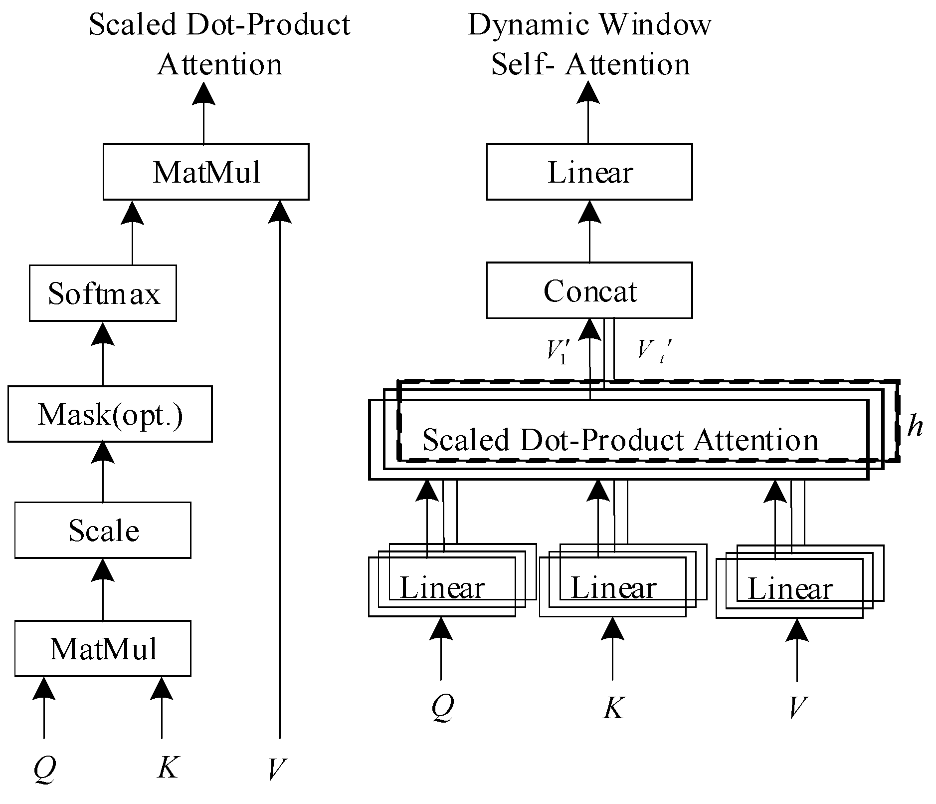
TED-Net is centered on the dynamic window self-attention mechanism. When processing long time-series data such as high-frequency trading data, the attention computation range becomes relatively large, leading to a significant increase in the computational burden of the model. To solve this problem, a dynamic window self-attention module is designed: instead of computing all attention with a fixed window in each feature-processing stage, the self-attentionrange is reasonably partitioned by dynamic windows, after which the self-attention computation is performed. After feature extraction, the raw high-frequency trading time-series data are transformed into the feature matrix, and the initial temporal feature X is fed into the dynamic window self-attention module. The Q, K, and V are obtained through linear transformations, as follows:
where WQ, WK, and WV are parameter matrices, and bQ, bK, and bV are bias matrices.
For each position , the dynamic window restricts the self-attention computation to within the dynamic window. The actual computation at position t is as follows:
where αt is the attention weight matrix, and is the final attention matrix.
A zero-padding strategy is adopted to complete the boundaries, ensuring that the attention computation range within the window is valid and that information at both ends of the sequence is not lost.
Concatenating the attention matrices computed by all dynamic windows yields the final output features of the dynamic window self-attention layer:
Figure 3.
Computational process of the dynamic window self-attention mechanism.
3. Experiments and Results Analysis
3.1. Feature Data Processing
Since financial data are non-stationary, nonlinear, and multi-scale, the extraction of effective information determines the prediction performance of deep learning models; therefore, valuable features must be extracted and transformed into a dataset for model training. Given that a high-dimensional sample set increases the correlation among features and thus prolongs model convergence time, PCA is selected for feature extraction and data dimensionality reduction, and a sample observation matrix is established for the initial data:
where n=19,200 is the number of samples and m=15 is the number of indicators. The correlation coefficient matrix is then constructed:
where
where rij is the correlation coefficient between the indicators xi and xj of the initial sample observations, representing the degree of association between the two indicators, and an d are the mean values of the indicators over all samples.
The eigenvalues λ and eigenvectors e of the correlation coefficient matrix in Equation (18) are computed, and the eigenvalues are sorted in descending order. The cumulative variance contribution rate of the principal components is then calculated. It reflects the expressive ability of the principal components with respect to the original information, the closer the value is to 1, the stronger the coverage of the original information by the currently extracted principal components.
Through PCA, seven reduced feature indicators are obtained: MACD = 0.78, TRIX = 0.69, VR = 0.76, OBV = 0.68, ROC = 0.75, MTM = 0.72, and PSY = 0.67 (their specific meanings are given in Table 1).
3.2. Model Parameter Settings
To verify the effectiveness and generalization ability of TED-Net, this paper selects minute-level high-frequency trading data of 15 A-share stocks from different industries and market capitalizations for experiments. For each stock, 24,000 one-minute data points are used as the experimental dataset; after data processing, the first 80% of samples are used as the training set and the last 20% as the validation set. The short-term sequence length is 30 minutes and the long-term sequence length is 120 minutes; the stock price data of the previous 30 minutes are used to predict the closing price of the next 1 minute. PCA is used for feature extraction and dimensionality reduction, and the required models are built with PyTorch.
A high-frequency trading prediction model is established with the prediction target set to the stock price for the next 1 minute. A 3-layer LSTM network structure is adopted. The loss function is the mean squared error (MSE) with L2 regularization; the learning rate is 0.007, the dropout rate is 0.03, and the activation function is tanh(x). The number of hidden units is set to 128, and the initial weights are randomly initialized from a normal distribution with mean 0 and variance 1. The input layer has 10 nodes (7 stock trading feature variables and 3 temporal variables), and the output layer has 1 node. The Adam optimization algorithm is used, with a batch size of 100 and a sequence length of 30.
3.3. Ablation Experiments
To systematically evaluate the effectiveness of each core component in the model and its contribution to overall performance, ablation experiments are designed to investigate the independent effects of the SAE feature encoder and the MSA correlation encoder on prediction ability. In addition, to comprehensively measure the overall performance of the optimized model in high-frequency trading trend prediction, four key evaluation metrics are selected: the Area Under the Curve (AUC), Precision, Recall, and F1-score (MF1). These metrics comprehensively reflect, from different dimensions, the effectiveness and reliability of the model in predicting market movement direction. The detailed experimental results are given in Table 2.
The experimental results show that the LSTM+Seq2Seq baseline model achieves an AUC of 0.83, demonstrating strong discriminative ability in the classification task; its precision is 95%, indicating a low false-positive rate; and its recall is 80%, showing that it can effectively identify genuine rising samples, although some misses remain. The MF1 value is 87%, balancing precision and recall. After adding the SAE feature encoder, all metrics improve, with the AUC increasing to 0.88 and the recall to 85%, indicating that feature purification helps the model capture more effective information. The complete TED-Net model (+SAE+MSA) achieves the best performance, with an AUC of 0.92, precision of 98%, and MF1 of 94%, reflecting the substantial contribution and influence of the SAE and MSA modules.
4. Comparative Experiments
To verify the effectiveness of TED-Net as a computational intelligence method in financial prediction, this paper comprehensively compares it with mainstream time-series models such as Transformer and TCN and analyzes the contribution of each module from the perspective of mathematical modeling.
Three time-series data-driven methods are instantiated, including TED-Net, Transformer, and temporal convolutional network (TCN). All networks are trained with the Adam algorithm, with dropout=0.1, learning rate=0.007, 800 training iterations, a target error of 10−5, one output-layer node, and eight input-layer nodes. For the TED-Net model, the encoder part is composed of 10 modules concatenated in series, each consisting of a 3-layer LSTM stack; the input consists of 3 temporal variables of stock indicators (day, hour, minute) plus 5 feature variables (open, high, low, close, and volume); the number of hidden units is set to 128; the initial states are all zero states; and the initial weights follow a normal distribution with mean 0 and variance 1. The decoder part of the model is also composed of 10 modules concatenated in series, each consisting of a 3-layer LSTM stack, with the tanh(x) activation function. For the Transformer model, the hyperparameters are feature length T=8, feature dimension dm=128, number of heads h=8, and 6 encoder/decoder layers. For the TCN, the kernel size is kernel_size=3, the dilation base is dilation_base=2, the number of residual blocks is num_residual_blocks=6, and the number of filters is num_filters=64.
To verify the generalization performance of the model, three experiments are conducted using minute-level high-frequency trading data of 15 typical stocks, with 8,000 samples in each experiment, as shown in Figure 4, where TRAN denotes the Transformer model. In the first experiment, compared with the Transformer model, TED-Net improves the accuracy on stocks ZX, XWF, AG, BJ, MR, TW, MY, and SX by 3.23%, 3.19%, 2.88%, 2.89%, 1.71%, 3.93%, 2.31%, and 2.95%, respectively; compared with the TCN model, except for a decrease of 1.71% on stock XWF, the improvements range from 1.89% to 17.08%. In the second experiment, compared with the Transformer and TCN models, TED-Net improves the accuracy on stock YS by 13.23% and 16.95%, respectively; except for improvements of 1.71% and 1.02% on stocks ZX and XWF for the TCN model, the remaining decreases range from 1.89% to 17.08%. In the third experiment, the accuracy of the Transformer on stock YS is 0.51% higher than that of TED-Net, while it is slightly lower than TED-Net on the other stocks; except for an improvement of 1.23% on stock XWF for the TCN model, the accuracy of the TCN is lower than that of TED-Net by margins ranging from 5.1% to 15.01%. The average prediction results are shown in Table 3. In summary, compared with the mainstream Transformer and TCN models, TED-Net exhibits varying degrees of performance improvement on most datasets, with particularly noticeable improvements on some individual stocks.
Using 39,604 one-minute data points of CATL stock quotes from 8 July 2025 to 13 March 2026 as the experimental dataset, with the first 80% of samples as the training set and the last 20% as the validation set, the prediction performance of TED-Net is analyzed. As shown in Figure 5(a), the optimal number of training epochs is determined from the loss curve to be 40, at which the loss converges and stabilizes at 0.00575 (finally 0.0054), indicating that the introduction of the SAE and the collaborative decoding mechanism significantly improves the convergence performance of the model on stock price data. Figure 5(b) shows the prediction results of TED-Net on the test set; it can be intuitively seen that the predicted price curve (red) and the real price curve (blue) follow essentially the same trend, and the model can accurately track the trend and direction even in intervals of frequent price fluctuations, demonstrating strong robustness and accuracy, although there remains an average error of 1.5 yuan. The same issue can also be observed from the scatter errors between the two curves in Figure 5(c); the reason is that, although standard LSTM can capture the nonlinear and temporal features of the data, it is limited by its local sequence modeling approach and finds it difficult to fully utilize global temporal information to construct the complex mapping between inputs and outputs. As shown in Figure 5(d), the error of 1.5 occurs with the highest frequency of 2,250, followed by the error of 1.0 with a frequency of 1,450 and the error of 2.5 with a frequency of 750. Overall, the error experimental data (see Table 4) show that the LSTM-Seq2Seq architecture in TED-Net effectively integrates full-sequence information through the encoder–decoder mechanism; moreover, the SAE feature encoder addresses the feature dilemma and, combined with the MSA, mines global dependencies, achieving good prediction accuracy, with an RMSE of 2.2292, an MAE of 2.0872, and an R² of 0.97, although there is still considerable room for model optimization.
5. Conclusions
In response to the three dilemmas of high-frequency trading data prediction, this paper proposes and validates the TED-Net hybrid deep learning model. Through theoretical analysis and experimental verification, the following main conclusions are drawn:
(1) An innovative “triple encoding-collaborative decoding” architecture is proposed. The three mechanisms of SAE feature encoding, LSTM temporal encoding, and MSA correlation encoding are organically integrated for the first time, and the core difficulties of high-frequency time-series prediction are systematically solved through the progressive learning process of “feature purification → temporal modeling → correlation enhancement → collaborative decoding”. Ablation experiments confirm that the addition of each module significantly improves model performance, and the complete model reduces the RMSE by 42.0% compared with the baseline, with an R² of 0.97.
(2) An attention-augmented collaborative decoding mechanism is designed. Gated fusion units are innovatively introduced to realize the adaptive integration of the triple encoding information, and an attention mechanism is introduced at the decoding end to dynamically focus on key historical information. This design effectively alleviates the information bottleneck of the fixed context vector in traditional Seq2Seq models and provides new insights into multi-source information fusion for complex time-series data.
(3) The superiority of the model in complex financial time-series prediction is verified. On million-level minute-frequency high-frequency datasets covering 15 stocks, the prediction accuracy of TED-Net comprehensively surpasses mainstream time-series models such as Transformer, TCN, and LSTM, with the average RMSE reduced by 16.2% compared with the Transformer, 17.6% compared with the TCN, and 22.9% compared with the LSTM. In the empirical analysis on CATL stock, the model achieves an excellent prediction result with R² = 0.97, verifying its outstanding adaptability in non-stationary, high-noise financial environments.
This study provides a systematic framework for high-frequency trading prediction in the field of computational finance. Future research will be devoted to exploring the combination of TED-Net with reinforcement learning to build an end-to-end high-frequency trading decision system and to further studying the interpretability of the model, so as to provide more valuable guidance for quantitative investment practice—this is precisely an important direction for the deepened application of computational intelligence methods in the financial field.
Author Contributions
Conceptualization, X.Z. and Y.Z.; methodology, X.Z.; software, X.Z. and H.Y.; validation, X.Z., M.Z., and Z.Z.; formal analysis, X.Z.; investigation, X.Z.; resources, Y.Z.; data curation, X.Z.; writing—original draft preparation, X.Z.; writing—review and editing, Y.Z.; visualization, X.Z.; supervision, Y.Z.; project administration, Y.Z.; funding acquisition, Y.Z. All authors have read and agreed to the published version of the manuscript. [Please confirm and adjust the specific contributions of each author.].
Funding
This research was funded by the National Major Science and Technology Project of Intelligent Manufacturing Systems and Robots, grant number 2025ZD1607900.
Data Availability Statement
The data presented in this study are available on request from the corresponding author.
Conflicts of Interest
The authors declare no conflicts of interest.
References
- Zhu, Z. The Origin, Development and Regulatory Considerations of International High-Frequency Trading [In Chinese]. China Secur. Futur. 2019, 3, 76–81. [Google Scholar]
- Wu, X.; Xu, R.; Sun, S. The Modern Financial System: Basic Characteristics and Functional Structure [In Chinese]. J. Renmin Univ. China 2020, 1, 60–73. [Google Scholar]
- Fischer, T.; Krauss, C. Deep Learning with Long Short-Term Memory Networks for Financial Market Predictions. Eur. J. Oper. Res. 2018, 270, 654–669. [Google Scholar] [CrossRef]
- Xie, X.; Lei, X.; Zhao, Y. Application of MI and Improved PCA Dimensionality Reduction Algorithms in Stock Price Prediction [In Chinese]. Comput. Eng. Appl. 2020, 56, 139–144. [Google Scholar]
- Wang, J. Prediction of Stock Price Reversal Points Based on BP Neural Network [In Chinese]. Mod. Comput. 2015, 5, 40–43. [Google Scholar]
- Shi, J.; Zou, J.; Zhang, J.; et al. Research on Stock Price Time-Series Prediction Based on the DMD-LSTM Model [In Chinese]. Appl. Res. Comput. 2020, 37, 662–666. [Google Scholar]
- Hargreaves, C.A.; Le Trung, H. Stock Prediction Using Sequence-to-Sequence Models. Financ. Innov. 2021, 7, 1–18. [Google Scholar]
- Deng, X.; Wan, L.; Huang, N. Stock Prediction Based on the DAE-BP Neural Network [In Chinese]. Comput. Eng. Appl. 2019, 55, 126–132. [Google Scholar]
- Vaswani, A.; Shazeer, N.; Parmar, N.; et al. Attention Is All You Need. In Proceedings of the 31st Conference on Neural Information Processing Systems (NeurIPS 2017), Long Beach, CA, USA, 4–9 December 2017; pp. 5998–6008. [Google Scholar]
- Wang, C.; Chen, Y.; Zhang, S.; et al. Stock Market Index Prediction Using Deep Transformer Model. Expert Syst. With Appl. 2022, 208, 118128. [Google Scholar] [CrossRef]
- Daiya, D.; Lin, C. Stock Movement Prediction and Portfolio Management via Multimodal Learning with Transformer. In Proceedings of the 2021 IEEE International Conference on Acoustics, Speech and Signal Processing (ICASSP), 2021; pp. 1–5. [Google Scholar]
- Berti, L.; Kasneci, G. TLOB: A Novel Transformer Model with Dual Attention for Stock Price Trend Prediction with Limit Order Book Data. arXiv 2025, arXiv:2502.15757. [Google Scholar]
- Barez, F.; Bilokon, P.; Gervais, A.; et al. Exploring the Advantages of Transformers for High-Frequency Trading. arXiv 2023, arXiv:2302.13850. [Google Scholar]
- Bai, S.; Kolter, J.Z.; Koltun, V. An Empirical Evaluation of Generic Convolutional and Recurrent Networks for Sequence Modeling. arXiv 2018, arXiv:1803.01271. [Google Scholar]
- Chan, S.Y. Explainable Multi-Step Time Series Forecasting Model. Thesis, Nanyang Technological University, Singapore, 2025. [Google Scholar]
- Suthi, G.; Kaladevi, P. A Hybrid Temporal-Spatial Deep Learning Model for High-Frequency Stock Market Prediction: A Systematic Review and Meta-Analysis. In Proceedings of the 2025 3rd International Conference on Artificial Intelligence and Machine Learning Applications (AIMLA), 2025; pp. 120–127. [Google Scholar]
- Zhang, J.; Ye, L.; Lai, Y. Stock Price Prediction Using CNN-BiLSTM-Attention Model. Mathematics 2023, 11. [Google Scholar] [CrossRef]
- Zhou, J.; Liu, C.; Liu, J. Stock Price Trend Prediction Model Integrating Channel and Multi-Head Attention [In Chinese]. Comput. Eng. Appl. 2025, 61, 324–338. [Google Scholar]
- Sang, S.; Li, L. A Novel Variant of LSTM Stock Prediction Method Incorporating Attention Mechanism. Mathematics 2024, 12, 945. [Google Scholar] [CrossRef]
- Chen, L.; Fan, X. TIC-FusionNet: A Multimodal Deep Learning Framework with Temporal Decomposition and Attention-Based Fusion for Time Series Forecasting. PLoS ONE 2025, 20, e0333379. [Google Scholar] [CrossRef] [PubMed]
- Ataei, S.; et al. Applications of Deep Learning to Cryptocurrency Trading: A Systematic Analysis. TechRxiv 2025. [Google Scholar] [CrossRef] [PubMed]
- Deep Learning for Algorithmic Trading: A Systematic Review of Predictive Models and Optimization Strategies. Results Eng. Authors missing in the source manuscript—please supply.. 2025, 26, 100390. [CrossRef]
- Sutskever, I.; Vinyals, O.; Le, Q.V. Sequence to Sequence Learning with Neural Networks. In Proceedings of the 28th Conference on Neural Information Processing Systems (NeurIPS 2014), Montreal, QC, Canada, 8–13 December 2014; pp. 3104–3112. [Google Scholar]
- Yu, C.; Li, M.; Yin, W. Stock Price Prediction Analysis Based on the PCA-BP Combined Model [In Chinese]. J. Chang. Univ. Sci. Technol. (Natural Science Edition) 2021, 44, 125–130. [Google Scholar]
- Giantsidi, S.; Tarantola, C. Deep Learning for Financial Forecasting: A Review of Recent Trends. Int. Rev. Econ. Financ. 2025, 104, 104719. [Google Scholar] [CrossRef]
Figure 1.
TED-Net encoder–decoder forecasting model.
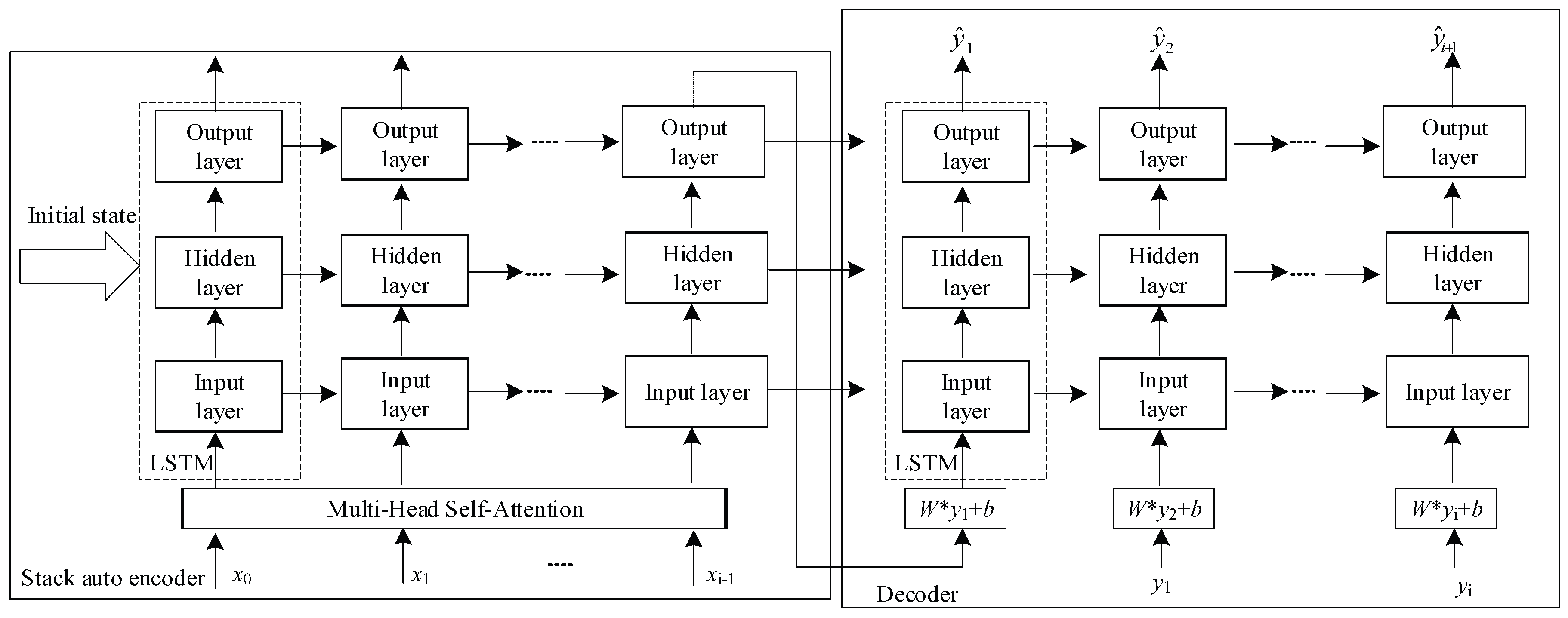
Figure 2.
LSTM-Seq2Seq deep learning model.
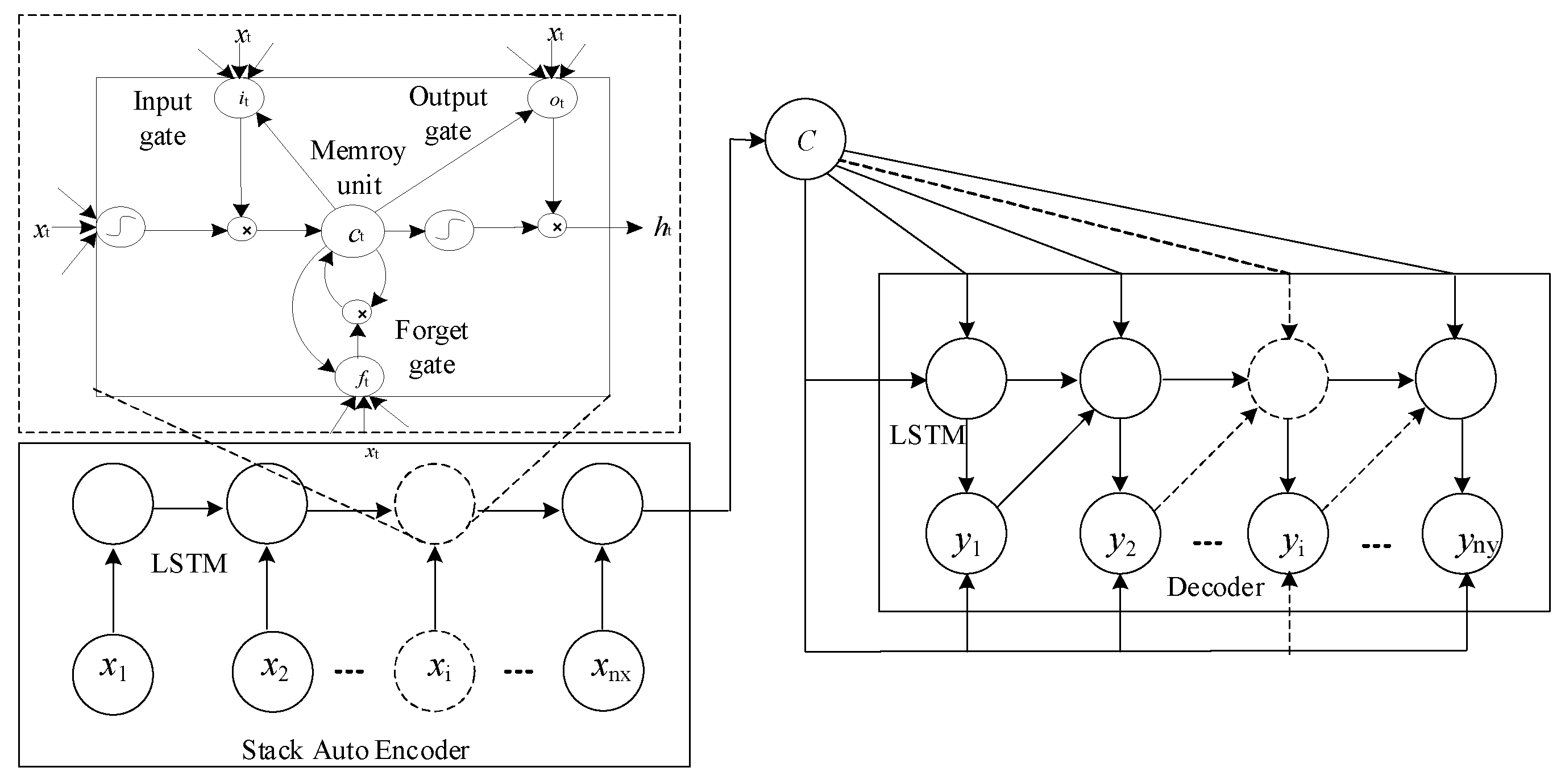
Figure 4.
Prediction accuracy comparison under three kinds of data-driven instances.
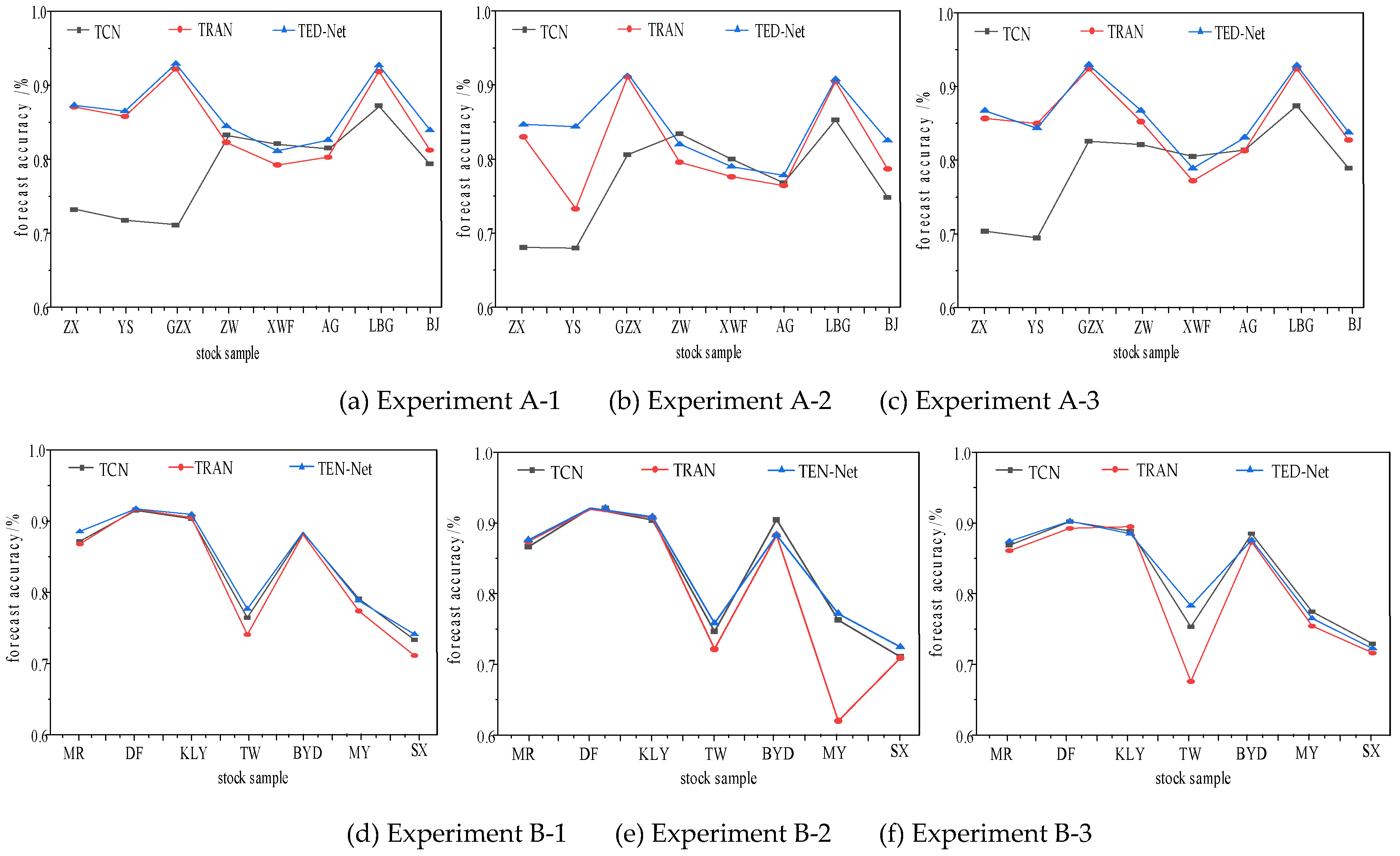
Figure 5.
High-frequency trading forecasting results on CATL stock.
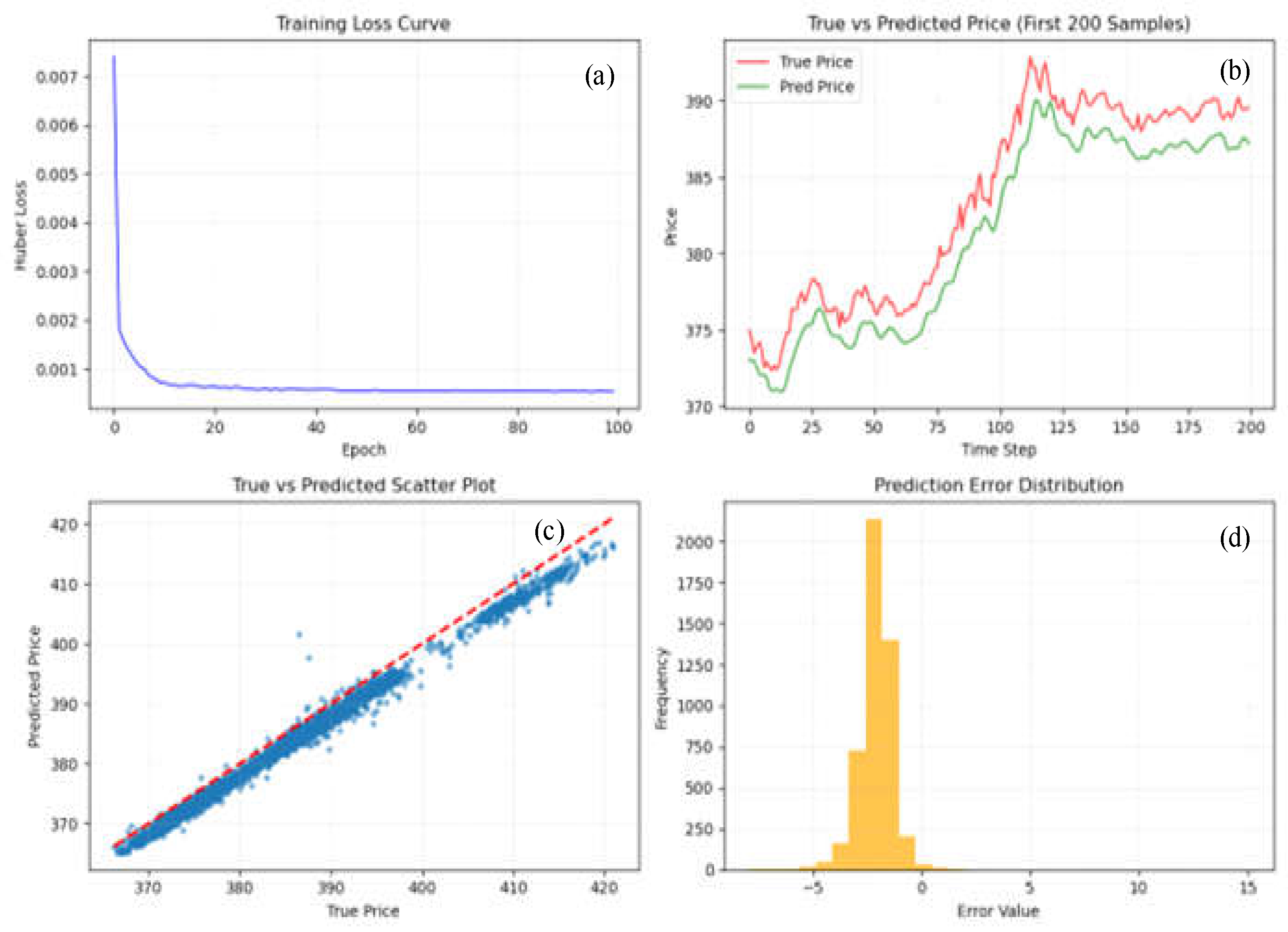

Table 1.
Model validation dataset and time-series database.
| Time | MACD | TRIX | VR | OBV | ROC | MTM | PSY |
|---|---|---|---|---|---|---|---|
| Date/Hour/Minute | Moving average convergence divergence | Triple exponential smoothing | Volume ratio | On-balance volume | Rate of change | Momentum | Investor sentiment |
| 2025/10/13-09:31 | -0.47 | -0.02 | 39.98 | 6503 | -1.84 | -7.01 | 41.67 |
| 2025/10/13-09:32 | -1.14 | -0.03 | 44.91 | 6503 | -1.63 | -6.18 | 41.67 |
| 2025/10/13-09:33 | -1.11 | -0.04 | 49.76 | 12823 | -1.06 | -4.02 | 41.67 |
| 2025/10/13-09:34 | -0.72 | -0.04 | 57.94 | 21139 | -0.39 | -1.49 | 50 |
| 2025/10/13-09:35 | -0.72 | -0.05 | 54.78 | 14887 | -0.9 | -3.43 | 50 |
| 2025/10/13-09:36 | -0.52 | -0.05 | 63.53 | 21213 | -0.55 | -2.1 | 58.33 |
| … | … | … | … | … | … | … | … |
| 2025/10/17-15:00 | 0.32 | -0.01 | 95.27 | -78790 | 0.2 | 0.71 | 41.67 |
Table 2.
Ablation study results.
| Model configuration | AUC | Precision | Recall | MF1 |
|---|---|---|---|---|
| Baseline: LSTM-Seq2Seq | 0.83 | 0.95 | 0.80 | 0.87 |
| +SAE feature encoder | 0.88 | 0.96 | 0.85 | 0.91 |
| +SAE+MSA correlation encoder (TED-Net) | 0.92 | 0.98 | 0.89 | 0.94 |
Table 3.
Prediction accuracy comparison on 15 stock datasets (%).
| No. | Symbol | Dataset | Transformer | TCN | LSTM-Seq2Seq | TED-Net |
|---|---|---|---|---|---|---|
| 1 | ZX | ZTE | 87.73 | 86.04 | 87.18 | 89.12 |
| 2 | YS | Yaguang | 86.66 | 86.60 | 84.19 | 88.34 |
| 3 | GZX | Gansu Consulting | 95.37 | 95.14 | 95.08 | 96.21 |
| 4 | ZW | Zhewen Pictures | 83.82 | 83.75 | 87.13 | 89.05 |
| 5 | XWF | New Wufeng | 79.24 | 80.19 | 77.14 | 81.43 |
| 6 | AG | Ansteel | 81.24 | 78.86 | 82.49 | 84.12 |
| 7 | LBG | Laobaigan | 95.06 | 94.23 | 94.97 | 96.33 |
| 8 | BJ | BNBM | 83.08 | 84.38 | 83.41 | 86.27 |
| 9 | MR | Mindray | 92.17 | 92.02 | 91.35 | 93.48 |
| 10 | DF | East Money | 96.79 | 96.63 | 96.91 | 97.82 |
| 11 | KLY | Asymchem | 95.63 | 93.72 | 95.37 | 96.55 |
| 12 | TW | Tongwei | 76.23 | 77.08 | 76.89 | 79.94 |
| 13 | BYD | BYD | 91.96 | 92.28 | 92.15 | 93.67 |
| 14 | MY | Muyuan | 78.03 | 74.10 | 78.58 | 80.21 |
| 15 | SX | Shanxi Coking | 71.13 | 68.28 | 72.79 | 75.06 |
Table 4.
Prediction performance comparison of the three models (CATL dataset).
| Model | RMSE | MAE | R² |
|---|---|---|---|
| LSTM | 3.4521 | 2.8910 | 0.92 |
| TCN | 3.2145 | 2.7234 | 0.93 |
| Transformer | 3.0876 | 2.6012 | 0.94 |
| TED-Net | 2.2292 | 2.0872 | 0.97 |
Disclaimer/Publisher’s Note: The statements, opinions and data contained in all publications are solely those of the individual author(s) and contributor(s) and not of MDPI and/or the editor(s). MDPI and/or the editor(s) disclaim responsibility for any injury to people or property resulting from any ideas, methods, instructions or products referred to in the content. |
© 2026 by the authors. Licensee MDPI, Basel, Switzerland. This article is an open access article distributed under the terms and conditions of the Creative Commons Attribution (CC BY) license (http://creativecommons.org/licenses/by/4.0/).
Copyright: This open access article is published under a Creative Commons CC BY 4.0 license, which permit the free download, distribution, and reuse, provided that the author and preprint are cited in any reuse.