

Submitted:
13 September 2026
Posted:
15 September 2026
Read the latest preprint version here
Abstract
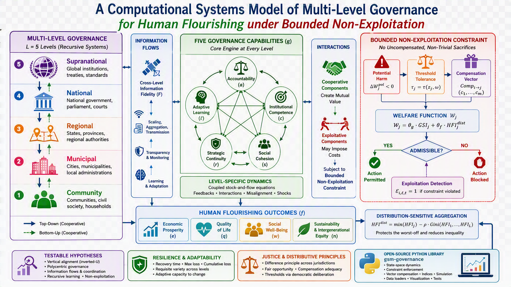
Governance operates simultaneously across multiple levels—from local communities to national governments to international institutions—yet most formal governance models treat governance as a single-level phenomenon and permit jurisdictions to advance their own flourishing at the expense of others. This conceptual paper extends the General Governance Success Model (GSM) to account for multi-level governance under a bounded non-exploitation constraint: no jurisdiction may impose uncompensated, non-trivial sacrifices on other jurisdictions for its own benefit. The extended model represents governance at L levels, each characterized by five coupled capabilities (accountability, institutional competence, social cohesion, strategic continuity, and adaptive learning). The framework formalizes vertical and horizontal interactions decomposed into cooperative and exploitative components, cross-level information flows with fidelity matrices, level-specific dynamics, recursive learning, and a formal non-exploitation constraint that admits both threshold tolerance and compensation as legitimate exceptions. A formal welfare function is specified, and the threshold parameter τj is decomposed into descriptive contextual variables and normative parameters. Compensation is modelled as a vector of transfers (fiscal, infrastructural, representational, regulatory, and future-oriented). A roadmap for operationalizing the exploitation index is provided. The model generates testable hypotheses concerning vertical alignment, polycentric governance, cross-level coordination, recursive learning, and non-exploitation. An illustrative worked example applying the GSM to Denmark—using real raw governance indicators but explicitly illustrative coefficients—is presented for pedagogical purposes, with comparative rankings relegated to a brief supplementary illustration. To support replication and application, the model is released as an open-source Python library, gsm-governance, which implements the state-space dynamics, bounded non-exploitation constraint, vector-valued compensation, threshold decomposition, and all reported indices. The extended GSM provides a foundation for analysing governance systems in their full institutional complexity while respecting normative constraints on inter-jurisdictional justice.
Keywords:
multi-level governance
; complex adaptive systems
; dynamical systems
; polycentric governance
; Viable System Model
; non-exploitation
; distributive justice
; human flourishing
; bounded rationality
1. Introduction
1.1. The Challenge of Multi-Level Governance
Governance does not occur at a single level. It operates simultaneously across nested scales: local communities, municipal governments, regional authorities, national states, and supranational institutions. Each level has distinct capabilities, constraints, and functions, yet they are deeply interconnected through vertical and horizontal relationships. Policy decisions at one level constrain or enable decisions at others; information flows across levels; legitimacy and accountability are distributed; and crises cascade through the system.
A critical but often neglected feature of this interconnectedness is that jurisdictions can impose costs on one another. A higher-level government may extract resources from lower-level jurisdictions; a lower-level jurisdiction may externalize environmental harms to neighbours; a peer jurisdiction may engage in regulatory competition that degrades collective welfare. In each case, one jurisdiction advances its own flourishing at the expense of others—a phenomenon we term jurisdictional exploitation.
Despite this multi-level reality, most formal governance models treat governance as a single-level phenomenon. Even frameworks that recognize multi-level structures rarely impose constraints on cross-jurisdictional harm. This simplification obscures the complexity of real governance systems and permits analytical frameworks that would endorse Pareto-improving exploitation—outcomes in which some jurisdictions gain by making others worse off.
1.2. The Computational and Systems Perspective
This paper extends the General Governance Success Model (GSM) to account for multiple levels of governance, subject to a bounded non-exploitation constraint: no jurisdiction may impose uncompensated, non-trivial sacrifices on other jurisdictions for its own benefit.
The GSM is a systems-theoretical metamodel that represents governance as a complex adaptive and information-processing system composed of five interacting institutional capabilities—accountability, competence, social cohesion, strategic continuity, and adaptive learning—whose dynamic configuration and contextual alignment determine the capacity of a governance system to promote sustainable human flourishing (Wang, 2026a).
The extension draws on six intellectual traditions:
- The Viable System Model (VSM): Beer's (1972, 1979) cybernetic framework for organizational viability is inherently recursive. Each level of governance contains the same essential functions as the whole.
- Polycentric Governance Theory: Ostrom (1990, 2010) and colleagues (Baldwin et al., 2024; Morrison et al., 2023) have demonstrated how multiple, interdependent centres of decision-making can address complex collective action problems—though they also recognize the risk of predatory behaviour among centres.
- Multi-Level Governance Theory: Hooghe and Marks (2001, 2003) developed the foundational framework for understanding governance across multiple levels.
- System Dynamics and Complex Adaptive Governance: Forrester's (1961, 1969) stock-and-flow modelling provides tools for understanding feedback processes. Building on this tradition, complex adaptive governance scholars (Holling, 2001; Gunderson & Holling, 2002; Folke et al., 2005) have examined how governance systems adapt to changing conditions.
- Network Governance: Provan and Kenis (2008) and Klijn and Koppenjan (2016) have demonstrated how network structures shape governance effectiveness.
- Distributive Justice and Federalism Theory: Rawls (1971), Sen (1999), and Nussbaum (2011) provide the normative foundations for the non-exploitation constraint. Extending these principles to the multi-level context, we draw on recent work in federalism and inter-jurisdictional justice (Sangiovanni, 2022; Miller, 2023; Young, 2023).
1.3. The Primary Contribution
The central contribution of this paper is a multi-level extension of the General Governance Success Model, subject to a bounded non-exploitation constraint. The extended model provides:
- A formal state-space representation of governance at multiple levels
- Vertical and horizontal interaction matrices decomposed into cooperative and exploitative components
- A formal welfare function that operationalizes the non-exploitation constraint
- 4.
- A bounded non-exploitation constraint with threshold tolerance and vector-valued compensation mechanisms
- 5.
- A formal decomposition of the threshold parameter separating descriptive context from normative choice
- 6.
- A roadmap for operationalizing the exploitation index
- 7.
- Multi-level information flows with fidelity across scales
- 8.
- Level-specific dynamics with differentiated parameters
- 9.
- Distribution-sensitive governance performance metrics that penalize exploitation
- 10.
- Testable hypotheses including hypotheses on non-exploitation
- 11.
- Falsifiability criteria
- 12.
- An illustrative worked example (Denmark) with real raw data and explicitly labeled illustrative coefficients
- 13.
- A publicly released computational implementation (gsm-governance; Wang, 2026b) that operationalizes the formal model, enables reproducibility of the worked example, and supports further empirical and simulation-based research.
The library is designed to be usable both pedagogically—for researchers who wish to reproduce the Denmark example and explore parameter sensitivity—and programmatically, for those who wish to embed the GSM in larger simulation environments. It provides separate modules for state representation, transition dynamics, constraint enforcement, welfare and index computation, and visualization, together with data loaders for the raw indicators drawn from V-Dem, the World Bank WGI, the World Justice Project, UNDP, and Our World in Data.
1.4. Research Questions
This paper addresses six principal research questions:
- How can governance systems be formally modelled at multiple levels?
- How do vertical and horizontal interactions shape governance performance?
- How do information flows and fidelity vary across governance levels?
- What conditions enable effective multi-level governance?
- How can multi-level governance performance be benchmarked and validated?
- How can the bounded non-exploitation constraint be formalized and enforced in a multi-level governance model?
2. Research Gap and Contribution
2.1. Limitations of Existing Governance Frameworks
Existing governance frameworks typically assume a single level of analysis. Democratic theory (Dahl, 1971; Mansbridge, 2003) focuses on national-level political institutions. State-capacity research (Evans, 1995; Fukuyama, 2013; Skocpol, 1985) examines national administrative effectiveness. Comparative political economy (Hall & Soskice, 2001; Rodrik, 2000) compares national institutional arrangements. Human-development research (Sen, 1999; Stiglitz et al., 2009; UNDP, 2022) measures national-level well-being.
Recent scholarship on polycentric governance (Baldwin et al., 2024; Morrison et al., 2023) and behavioural public administration (Grimmelikhuijsen et al., 2017; Jilke et al., 2024; Alon-Barkat & Busuioc, 2024) has advanced understanding of governance dynamics. However, none of these frameworks systematically constrain jurisdictions from imposing costs on one another. Justice-and-federalism scholarship (Sangiovanni, 2022; Miller, 2023; Young, 2023) has advanced normative principles for inter-jurisdictional relations but has not embedded these in computational governance models.
2.2. The Systems and Cybernetics Heritage

Table 1.
Viable System Model (VSM) to GSM Dimension Mapping.
| VSM System | Function | GSM Dimension (Analogue) |
| System 1: Implementation | Operational capability | Competence |
| System 2: Coordination | Conflict resolution and oscillation control | Social Cohesion |
| System 3: Control | Monitoring, oversight, and resource allocation | Accountability |
| System 4: Intelligence | Environmental scanning and strategic intelligence | Adaptive Learning |
| System 5: Policy | Strategic direction and normative closure | Strategic Continuity |
Clarification on the Mapping: The GSM dimensions are conceptual analogues rather than direct one-to-one equivalents of VSM systems. The VSM is an organizational cybernetic framework, while the GSM addresses societal governance. The mapping captures functional correspondences while acknowledging that societal governance involves democratic, behavioural, and normative properties not contained in the organizational VSM. This mapping has been further developed by cyberneticians such as Espejo (1994, 2003), Schwaninger (2004, 2006), and Jackson (2000, 2003).
2.3. Polycentric Governance
Ostrom's (1990, 2010) polycentric governance theory describes systems with multiple, interdependent centres of decision-making. Crucially, polycentric systems can also generate predatory dynamics. When decision centres compete for resources, authority, or legitimacy, they may engage in behaviour that harms other centres. The multi-level GSM addresses this through the non-exploitation constraint formalized in Section 4.6.
2.4. Multi-Level Governance Theory
Hooghe and Marks (2001, 2003) developed the foundational framework for multi-level governance, distinguishing between Type I (general-purpose, non-overlapping jurisdictions) and Type II (task-specific, overlapping jurisdictions) governance arrangements.
2.5. Complex Adaptive Governance
Building on system dynamics and resilience theory (Holling, 1973, 2001; Gunderson & Holling, 2002), complex adaptive governance scholars (Folke et al., 2005; Levin et al., 2013) have examined how governance systems adapt to changing conditions. Recent resilience-governance reviews (Morgan et al., 2023; Saikia & Jiménez, 2023) provide additional insight.
2.6. Network Governance
Network governance research (Rhodes, 1996; Provan & Kenis, 2008; Klijn & Koppenjan, 2016) examines how policy networks shape governance outcomes. The bounded non-exploitation constraint is a normative requirement on network interactions that prevents powerful actors from leveraging network position to extract value from weaker actors.
2.7. Human Flourishing and Well-Being Research
The flourishing dimension builds on established frameworks: Sen's (1999) capability approach, Nussbaum's (2011) central capabilities, OECD (2022) Better Life Index, UNDP (2022) Human Development Index, and the Stiglitz Commission (Stiglitz et al., 2009).
The four flourishing dimensions () are not claimed to be exhaustive. They represent a parsimonious synthesis of broader flourishing frameworks selected for analytical tractability while maintaining conceptual breadth.
Table 2.
Flourishing Dimensions and Theoretical Foundations.
| Dimension | Definition | Theoretical Foundation | Operationalization |
| Economic Prosperity () | Material well-being, income, employment | Sen (1999), Stiglitz et al. (2009) | GDP per capita, median income, employment rate |
| Quality of Life () | Health, education, subjective well-being | Nussbaum (2011), OECD (2022) | Life expectancy, educational attainment, happiness |
| Social Well-Being () | Trust, safety, opportunity, inclusion | Putnam (1993), Rothstein (2011) | Social trust, safety perceptions, equality |
| Sustainability () | Environmental quality, intergenerational equity | UNDP (2022), Brundtland Commission | Environmental performance, resource efficiency |
2.8. The Computational Gap
Despite these advances, the literature lacks:
- A formal computational framework for multi-level governance
- Explicit representations of vertical and horizontal interactions
- Formal models of cross-level information flows
- Testable hypotheses about multi-level governance dynamics
- A formal welfare function and bounded constraint prohibiting jurisdictions from sacrificing other jurisdictions for their own benefit
2.9. Why Existing Multi-Level Governance Theory Is Not Enough
Table 3.
Comparison of Multi-Level Governance Frameworks.
| Feature | MLG Theory | Polycentric Governance | VSM | Multi-Level GSM |
| Multi-level structures | ✓ | ✓ | ✓ | ✓ |
| Dynamic feedbacks | Limited | Partial | ✓ | ✓ |
| Computational formalization | ✗ | Limited | ✓ | ✓ |
| Information fidelity | ✗ | ✗ | ✗ | ✓ |
| Recursive learning | ✗ | Limited | ✓ | ✓ |
| Human flourishing outcomes | ✗ | ✗ | ✗ | ✓ |
| Non-exploitation constraint | ✗ | ✗ | ✗ | ✓ |
| Distribution-sensitive aggregation | ✗ | ✗ | ✗ | ✓ |
3. Multi-Level State-Space Representation
3.1. Level-Indices and Hierarchical Structure
Define a hierarchy of governance levels . For analytical tractability, the model uses a standard five-level hierarchy: community, municipal, regional, national, and supranational governance.
For each level , define the governance state vector:
where represent accountability, competence, social cohesion, strategic continuity, and adaptive learning respectively.
Table 4.
Governance Capabilities Across Five Levels of Governance.
| Capability | Level 1: Community | Level 2: Municipal | Level 3: Regional | Level 4: National | Level 5: Supranational |
| Accountability | Community meetings, local elections | City councils, local audits | Regional assemblies, state oversight | National parliament, judicial review | International treaties, UN mechanisms |
| Competence | Local service delivery | Urban planning, public works | Regional coordination | National policy, administration | Global coordination, standard-setting |
| Social Cohesion | Neighbourhood trust | City identity | Regional identity | National identity | International cooperation |
| Strategic Continuity | Local plans | City master plans | Regional strategies | National visions | Global frameworks |
| Adaptive Learning | Local experimentation | City innovation | Regional adaptation | National reform | Global learning |
3.2. Level-Specific Feasible Spaces with Non-Exploitation Constraint
Each level has its own feasible state space:
where:
- represents coupling, resource, institutional, legal, and normative constraints
- represents the bounded non-exploitation constraint (defined formally in Section 4.6)
3.3. Level-Specific Flourishing
Define flourishing outcomes at each level:
4. Design Principles of the Multi-Level GSM
4.1. Recursion Principle
Derived from Beer's (1972) VSM and elaborated by Espejo (1994, 2003) and Schwaninger (2004, 2006): each governance level contains the same five essential functions as the whole.
4.2. Coordination Principle
Derived from polycentric governance (Ostrom, 1990) and network governance (Provan & Kenis, 2008): effective multi-level governance requires both vertical and horizontal coordination.
4.3. Information Principle
Derived from Ashby's (1956) Law of Requisite Variety: governance performance depends on information processing capacity across levels.
4.4. Adaptation Principle
Derived from complex adaptive governance (Holling, 2001; Folke et al., 2005): governance systems must adapt to changing conditions.
4.5. Flourishing Principle
Derived from Sen (1999), Nussbaum (2011), and well-being research: the ultimate objective of governance is sustainable human flourishing.
4.6. The Bounded Non-Exploitation Principle
The central normative innovation of this paper is the bounded non-exploitation principle, derived from Rawls (1971), Sen (1999), Nussbaum (2011), and recent work in federalism and inter-jurisdictional justice (Sangiovanni, 2022; Miller, 2023; Young, 2023):
Bounded Non-Exploitation Principle: No jurisdiction may advance its own governance capabilities or flourishing outcomes by imposing uncompensated, non-trivial sacrifices on other jurisdictions. Each jurisdiction's actions must be constrained to those that either (a) leave every other jurisdiction no worse off, or (b) impose only sacrifices below a socially accepted threshold, or (c) impose sacrifices that are adequately compensated.
4.6.1. Formal Definition of Jurisdictional Welfare
To operationalize the non-exploitation constraint, we first define a formal welfare function for each jurisdiction:
where:
- is the governance success index for jurisdiction at time
- is the distribution-sensitive human flourishing index for jurisdiction
- are normative weights with
Note on Welfare Aggregation Overlap: A reviewer might reasonably ask whether governance quality is being "double-counted" in this specification, since already influences through the dynamics. We retain the dual-index specification for two reasons. First, governance quality may have intrinsic normative significance independent of outcomes: citizens may value living under accountable, competent institutions even if those institutions have not yet produced improvements in flourishing. Second, the two components capture distinct temporal dimensions: reflects current institutional capability, while reflects realized (and distribution-sensitive) outcomes. Alternative welfare specifications may rely exclusively on flourishing outcomes (); this remains a normative choice for the relevant political community.
Future empirical work should compare alternative welfare definitions through out-of-sample predictive validation and stakeholder deliberation, assessing whether single-index, dual-index, vector-valued, or capability-based welfare specifications produce systematically different judgments about exploitation, compensation adequacy, and constraint enforcement. This comparative exercise would help identify which welfare specifications are most robust across contexts and most consistent with democratic legitimacy.
Alternative welfare specifications:
- Single-index welfare: (flourishing-only)
- Vector welfare: with lexicographic or Pareto ordering
- Capability-based welfare: (weakest capability)
- Weighted capability welfare:
The choice of welfare specification is a normative decision subject to democratic deliberation (Section 10.4).
4.6.2. Bounded Non-Exploitation Constraint
For any jurisdiction at level contemplating action , the action is admissible if and only if at least one of the following conditions holds. Throughout, the counterfactual baseline is defined as the welfare that would have obtained had the action not been taken, i.e., — not the current welfare — so that policy effects are isolated from unrelated time trends.
Condition A (Weak Non-Exploitation — No Harm):
Condition B (Threshold Tolerance):
where is a socially accepted threshold for jurisdiction representing the maximum acceptable short-term sacrifice relative to the no-action counterfactual.
Condition C (Compensation):
where is the effective compensation transferred from jurisdiction to jurisdiction , defined in Section 4.6.5 as:
with the recipient-specific valuation vector and the vector of compensation transfers.
Combined Constraint:
The bounded non-exploitation constraint can be stated compactly as:
Equivalently, defining the policy-induced welfare change as
the constraint is:
Why the counterfactual baseline matters. Comparing post-action welfare to current welfare, , conflates three distinct effects: (a) the policy's impact, (b) underlying trends in welfare that would have occurred regardless (e.g., demographic change, exogenous economic growth, environmental drift), and (c) cyclical noise. Only (a) is attributable to the action. Using as the baseline isolates (a). This baseline is not directly observable in any single time series but can be estimated in empirical applications via synthetic controls, difference-in-differences, or model-based counterfactuals — a task identified in Section 15.7 as a priority for empirical work.
4.6.3. Rationale for the Bounded Formulation
The absolute version of the non-exploitation constraint (Condition A alone) is normatively attractive but empirically impractical. Governance inevitably involves trade-offs:
- Environmental policy: A carbon tax may benefit future generations and national resilience while imposing immediate costs on specific regions, workers, and industries.
- Infrastructure: Building a rail corridor may improve aggregate welfare while reducing welfare for specific local communities during construction.
- Public health: Pandemic restrictions inevitably harm some groups more than others.
The bounded formulation recognizes that not all negative externalities constitute exploitation. Exploitation occurs only when:
- The sacrifice exceeds the socially accepted threshold (), and
- Compensation is inadequate.
This aligns with Rawls's (1971) difference principle and with recent federalism theory (Sangiovanni, 2022).
4.6.4. Formal Determination of the Threshold Parameter
The threshold is decomposed into descriptive contextual variables and normative parameters:
where:
- is a vector of contextual variables for jurisdiction (e.g., development level, wealth, historical precedents, sectoral exposure)
- is a vector of normative parameters (e.g., acceptable harm thresholds, equity weights, deliberative outcomes)
This decomposition separates:
- Descriptive context — which can be estimated empirically from historical, institutional, and economic data
- Normative choice — which must be determined through democratic deliberation
The functional form may be specified as:
where the coefficients are determined by deliberative processes and the are observable contextual variables. This allows for empirical estimation of the contextual component while preserving the normative component as a matter of explicit political choice.
The threshold may vary across jurisdictions, sectors, and time horizons. For example, wealthier jurisdictions may have lower tolerance for exploitation (smaller ), while developing jurisdictions may accept higher thresholds in exchange for development opportunities.
4.6.5. Vector-Valued Compensation
Compensation is modelled as a vector of transfers rather than a single scalar:
where the components capture distinct compensation types:
| Component | Symbol | Description |
| Fiscal transfers | Direct payments from exploiting to exploited jurisdictions | |
| Infrastructure investment | Roads, bridges, ports, digital infrastructure, or energy systems | |
| Representation rights | Enhanced voice in decision-making, veto rights, or consultative status | |
| Regulatory accommodation | Exemptions, flexibilities, or differential rules | |
| Future commitments | Binding obligations to provide future benefits | |
| Restitutional benefits | Repair for past harms or lost opportunities |
The vector structure allows for:
- Compensation adequacy to become testable: does the combination of compensation types fully offset the harm, judged by the affected jurisdiction's own welfare function?
- Compensation heterogeneity to be modelled: some jurisdictions may prefer fiscal transfers while others prioritize representation or regulatory relief.
- Compensation composition to be optimized in bargaining processes.
The effective compensation is computed as a welfare-weighted combination:
where is a recipient-specific weighting vector reflecting jurisdiction 's own valuation of each compensation type.
Determination of the Compensation Valuation Vector:
The valuation vector is a critical parameter that determines how compensation is assessed. Its determination is itself a normative question that admits four possible mechanisms, each with distinct institutional implications:
Recipient declaration (chosen by jurisdiction). The affected jurisdiction declares its own valuation of each compensation type. This respects recipient sovereignty and aligns with the principle that compensation adequacy should be evaluated from the recipient's perspective. However, it creates a strategic incentive for recipients to overstate their valuation of compensation types they expect to receive, potentially leading to over-compensation demands.
Judicial determination (set by courts or tribunals). An independent judicial body determines the appropriate valuation based on precedent, expert testimony, and evidentiary standards. This mechanism is analogous to damages assessment in tort law and has the advantage of neutrality and enforceability. However, courts may lack the contextual knowledge to assess jurisdiction-specific valuations, and judicial processes may be slow and costly.
Bargaining (negotiated betweenand). The exploiting and exploited jurisdictions negotiate the valuation vector directly. This is consistent with polycentric governance principles of self-organization and mutual adjustment. However, asymmetric bargaining power may lead to outcomes that favor stronger parties, undermining the protective intent of the non-exploitation constraint.
Empirical estimation (estimated from revealed preferences or stated-preference surveys). The valuation vector is estimated using econometric methods (e.g., discrete choice experiments, hedonic pricing, contingent valuation). This approach has the advantage of being grounded in observed behavior or systematically elicited preferences, but it requires substantial data and may not capture values that are difficult to monetize (e.g., cultural or symbolic compensation).
Hybrid Approach: In practice, the GSM framework recommends a hybrid approach: the recipient's declared valuation serves as a baseline, subject to a reasonableness review by an independent body that may adjust for demonstrable over- or under-statement. This mirrors existing institutional arrangements in international investment arbitration, where claimants' valuations are subject to independent assessment. Formally:
where is a weight determining the relative influence of recipient declaration versus independent assessment. The weight itself is a normative parameter subject to the same democratic deliberation processes as the threshold (Section 4.6.4).
Future empirical work should test the practical implementation of these alternative determination mechanisms in specific governance contexts (e.g., federal transfers, international climate finance, water sharing agreements) to identify which mechanisms best satisfy the joint criteria of fairness, enforceability, and efficiency.
Compensation Adequacy: Compensation is adequate if:
where is the welfare change experienced by jurisdiction .
4.6.6. Compensation Adequacy
Compensation adequacy is evaluated based on the affected jurisdiction's own welfare function, not the exploiting jurisdiction's assessment. Formally, compensation is adequate if:
where is the welfare change experienced by jurisdiction .
4.7. Justice and Distributional Considerations
Following Rawls (1971) and recent federalism scholarship (Sangiovanni, 2022; Miller, 2023; Young, 2023), we recognize:
- Inequalities are permitted only if they benefit the least advantaged.
- Fair equality of opportunity applies across jurisdictions.
- The difference principle extends to inter-jurisdictional relations.
- Compensation is a legitimate mechanism for inter-jurisdictional justice.
5. Vertical and Horizontal Interactions with Exploitation Terms
5.1. Vertical Interaction Matrices
Top-Down Influence:
Bottom-Up Influence:
Combined vertical influence:
5.2. Decomposition of Vertical Interactions
We decompose vertical interactions into cooperative and exploitative components:
The bounded non-exploitation constraint requires that exploitative vertical interactions satisfy Conditions A, B, or C.
5.3. Horizontal Interaction Matrices
5.4. Decomposition of Horizontal Interactions5.5. Integrated Interaction Structure
5.5. Integrated Interaction Structure
Exploitative components are removed unless Conditions A, B, or C are satisfied.
6. Multi-Level Information Flows
6.1. Information-Flow Matrix
with block structure distinguishing intra-level and cross-level flows.
6.2. Information Fidelity Across Levels
Fidelity may vary due to transmission distortion, latency, granularity, bias, loss, and strategic misrepresentation.
Information and Non-Exploitation: High-fidelity information flows are a prerequisite for detecting exploitation.
6.3. Information Processing Capacity
7. Multi-Level Governance Dynamics
7.1. Coupled Dynamic System
where is restricted to the bounded non-exploitation feasible set, and projects onto the feasible space including the bounded non-exploitation constraint.
7.2. Coupled Flourishing Dynamics
7.3. Cross-Level Flourishing Spillovers
Cooperative spillovers:
Exploitative spillovers are permitted only if Conditions A, B, or C are satisfied.
7.4. Level-Specific Misalignment
7.5. Vertical Misalignment: Constructive vs. Destructive
The relationship between vertical misalignment and performance follows an inverted-U curve:
Constructive misalignment arises from federalism, separation of powers, polycentric governance, and pluralism. Destructive misalignment arises from policy incoherence, conflicting mandates, excessive fragmentation, coordination failures, and exploitation of one jurisdiction by another.
7.6. Exploitation Detection and Correction
Define the exploitation detection function at each level, using the counterfactual baseline and effective compensation:
Equivalently, in terms of the policy-induced welfare change :
When exploitation is detected (), the correction mechanisms described in the paper activate:
- Automatic constraint enforcement: Projection removes exploitative actions from the feasible set.
- Compensation requirement: The exploiting jurisdiction must provide adequate compensation.
- Accountability response: Higher-level accountability mechanisms may be activated.
- Information disclosure: Exploitation is made visible to affected parties.
8. Multi-Level Governance Performance
8.1. Level-Specific Governance Success
8.2. Level-Specific Governance Success
8.3 Distribution-Sensitive Aggregation
8.4. Level-Specific Human Flourishing
8.5. Aggregated Human Flourishing with Bounded Non-Exploitation
9. Causal-Loop Diagram
Figure 1.
Causal-Loop Diagram of the Multi-Level GSM with Bounded Non-Exploitation Constraint.
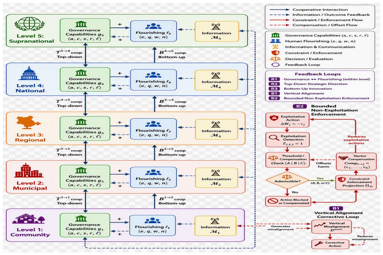
Defined Loops:
R1: Governance-Flourishing Reinforcement (Within Level)
R2: Top-Down Strategic Direction (Cooperative)
R3: Bottom-Up Innovation
B1: Vertical Alignment
B2: Bounded Non-Exploitation Enforcement
10. Multi-Level Equilibrium and Stability
10.1. Equilibrium Conditions
A multi-level equilibrium for all satisfies:
where is the reference target profile at equilibrium (this replaces the earlier notation , which was a typographic artifact).
Note: The equilibrium is constrained by the bounded non-exploitation requirement. Equilibria that violate the constraint are not admissible unless compensation satisfies Conditions B or C.
10.2. Stability Conditions
Local stability requires where is the block-structured Jacobian.
10.3. Multiple Equilibria Across Levels
Multiple equilibria may arise from threshold effects, institutional complementarities, path dependence, lock-in effects, and regime switching. Non-exploitation and equilibrium selection: Among multiple possible equilibria, the bounded non-exploitation constraint selects for Pareto-efficient, non-exploitative configurations.
11. Multi-Level Control Architecture
11.1. Hierarchical Control with Recursion
Table 5.
Hierarchical Control Architecture.
| GSM Level | VSM System | Function | Time Horizon |
| Level 5: Supranational | System 5 (Policy) | Global policy coordination | 20–50 years |
| Level 4: National | System 4 (Intelligence) | Strategic direction | 10–30 years |
| Level 3: Regional | System 3 (Control) | Policy implementation | 5–15 years |
| Level 2: Municipal | System 2 (Coordination) | Coordination | 3–10 years |
| Level 1: Community | System 1 (Implementation) | Service delivery | 0–5 years |
11.2. Control Variables at Each Level
restricted to the bounded non-exploitation feasible set.
11.3. Coordination Mechanisms with Bounded Non-Exploitation
Top-down, bottom-up, and peer coordination mechanisms are restricted to cooperative components, with exploitative components subject to Conditions A, B, or C.
12. Multi-Level Resilience and Adaptability
12.1. Level-Specific Resilience Metrics
Recovery time, maximum performance loss, and cumulative loss are defined as before.
12.2. Systemic Resilience
12.3. Adaptability Across Levels
Level-specific and systemic adaptability are defined as before.
13. Multi-Level Requisite Variety
13.1. Level-Specific Variety
Governance response variety and environmental variety are defined as entropy measures.
13.2. Requisite Variety Condition
13.3. Multi-Level Requisite Variety with Non-Exploitation
The bounded non-exploitation constraint requires sufficient regulatory variety to detect and prevent exploitation.
14. Multi-Level Hypotheses
H1: Optimal Vertical Differentiation
H2: Level-Specific Capability Balance
H3: Vertical-Horizontal Interaction
H4: Polycentric Governance Advantage
H5: Information Flow and Coordination
H6: Recursive Learning
H7: Bounded Non-Exploitation and Governance Performance
H7a:; prediction: .
H7b:; prediction: .
H7c:; prediction: , .
H8: Non-Exploitation and Systemic Resilience
H9: Compensation Effectiveness
Prediction: (compensation offsets harm).
H10: Threshold Sensitivity
The threshold parameter does not have a theoretically determinate sign for the exploitation–flourishing relationship. A larger loosens the constraint, admitting a broader class of actions as formally admissible; it does not, by itself, reduce the substantive harm those actions cause. Two effects may therefore pull in opposite directions:
- Permissiveness effect: Larger permits more actions with negative externalities, which may increase observed exploitation and harm.
- Classification effect: Larger reclassifies borderline harmful actions as non-exploitative, which may reduce the measured exploitation index conditional on the same underlying conduct.
The net effect is an empirical question. We therefore specify H10 as a testable relationship with an indeterminate predicted sign:
Prediction: The sign of is theoretically indeterminate and must be determined empirically. A positive would indicate that larger thresholds attenuate the negative effect of measured exploitation on flourishing (consistent with the classification effect dominating); a negative would indicate that larger thresholds amplify the negative effect (consistent with the permissiveness effect dominating). Distinguishing these mechanisms is a priority for future empirical work.
15. Multi-Level Benchmarking and Validation
15.1. Governance Success Index
15.2. Aggregated Governance Success Index
15.3. Human Flourishing Index
15.4. Distribution-Sensitive Aggregation
15.5. Primary Validation Design
Methodological Clarification: The empirical validation of the GSM framework has not yet been conducted. Empirical validation would require the following steps:
Unit of analysis: Country-year with subnational units
Period: 2000–2025 (multidecade panel)
Governance constructs: Latent variables or transparent composite measures at each level
Outcome: Multidimensional flourishing at each level, plus exploitation measures
Primary model: Dynamic panel or Bayesian multilevel model with cross-level interactions
Baseline comparison: Single-level governance model
Validation: Temporal and geographic holdout samples
Required Empirical Estimation Steps:
- Assemble a multi-country, multi-year panel of GSM dimension scores from V-Dem, WGI, WJP, UNDP, and other sources.
- Test measurement invariance across countries and time (Vandenberg & Lance, 2000; Putnick & Bornstein, 2016).
- Estimate via confirmatory factor analysis.
- Estimate via interaction regression with cross-validation.
- Estimate via public preference surveys or expert elicitation.
- Estimate via democratic deliberation.
- Estimate contextual target profiles using nested cross-fitting.
- Develop an exploitation index (see Section 15.7).
- Test predictive validity on held-out countries and years.
- Report out-of-sample performance metrics (RMSE, MAE, R²).
15.6. Falsification Criteria
The multi-level GSM would be challenged if:
- Level irrelevance: Higher-level governance shows no independent effect on flourishing.
- Vertical alignment irrelevance: Vertical misalignment shows no relationship with performance.
- Horizontal coordination irrelevance: Peer-level coordination shows no positive relationship with performance.
- Polycentricity non-monotonicity: Performance shows a strictly monotonic relationship with polycentricity.
- Information flow irrelevance: Cross-level information flow shows no moderating effect.
- Recursive learning absence: Learning at one level does not predict learning at other levels.
- Level-specific heterogeneity absence: The optimal balance of capabilities does not vary across levels.
- Non-exploitation irrelevance: Exploitation shows no relationship with aggregate or worst-off flourishing.
- Compensation irrelevance: Compensation shows no relationship with the exploitation-flourishing relationship.
- Threshold irrelevance: The threshold parameter shows no moderating effect.
Note on Supplementary Material: The illustrative comparative rankings that would ordinarily appear in Appendix C have been moved to the online supplementary material to keep the main text focused on the theoretical and methodological contributions of the GSM framework. Readers interested in the illustrative demonstration of the GSM methodology across multiple countries should consult the supplementary document, which also contains the full 50-country hypothetical ranking table, detailed regional analyses, and extended discussion of the governance failure patterns. The main text retains only the conceptual framework, the formal model, and the Denmark worked example.
15.7. Roadmap for Operationalizing the Exploitation Index
The exploitation index does not yet exist empirically. Development of such an index is a priority for future research. A preliminary decomposition is proposed:
where:
| Component | Symbol | Description | Candidate Indicators |
| Environmental externalization | Cross-border pollution, carbon leakage, resource depletion | Net carbon imports, transboundary pollution flows | |
| Fiscal extraction | Resource extraction, tax avoidance, subsidy capture | Terms-of-trade effects, transfer pricing, subsidy asymmetry | |
| Regulatory dumping | Race-to-the-bottom regulatory competition | Labour standards, environmental standards, corporate tax rates | |
| Institutional domination | Voting power asymmetries in international institutions | IMF/World Bank voting shares, trade negotiation asymmetry | |
| Temporal exploitation | Imposing costs on future generations | Debt-to-GDP ratios, resource depletion rates, climate commitments |
The weights are provisional and subject to empirical calibration. Their initial values should be determined through a combination of:
- Expert elicitation from international economics, environmental science, and political science
- Empirical analysis of historical cases where exploitation is well-documented (e.g., colonial extraction, asymmetric trade agreements)
- Democratic deliberation to ensure the weighting reflects societal values regarding different forms of exploitation
- Cross-validation against outcomes to identify which weighting structures best predict variation in flourishing
The provisional nature of these weights should be explicitly acknowledged in any empirical application. Sensitivity analysis across alternative weightings should be a standard component of future validation work. We anticipate that the appropriate weights will vary across contexts—for example, environmental externalization may be weighted more heavily in climate-vulnerable regions, while fiscal extraction may be weighted more heavily in resource-dependent economies.
15.8. Computational Implementation: The gsm-governance Library
The formal model presented in Section 3, Section 4, Section 5, Section 6, Section 7 and Section 8 is implemented in the open-source Python package gsm-governance (Wang, 2026b). The library provides a complete, executable realization of the GSM, structured to mirror the theoretical decomposition of the paper.
Design principles. The library is organized into five modules that correspond directly to the analytical sections:
| Library module | Corresponding paper section | Purpose |
| core | §3, §4 | State vectors, parameters, multi-level system container |
| dynamics | §5, §6, §7 | Transition equations, information flows, constraint enforcement |
| metrics | §8, §12 | GSI, HFI, distribution-sensitive aggregation, welfare, resilience |
| data | §15.5, §16.2 | Loaders for V-Dem, WGI, WJP, UNDP, OWID indicators |
| utils | §16.3 | Normalization, visualization |
Core formal elements implemented.
- The five-dimension governance state and the four-dimension flourishing state are represented by GovernanceState and FlourishingState classes (Section 3).
- The information-flow and fidelity matrices and are represented as NumPy arrays, with effective flow computed as (Section 6).
- The coupled transition equations (1) and (2) are implemented in TransitionModel.step_governance and TransitionModel.step_flourishing (Section 7).
- The bounded non-exploitation constraint (Conditions A, B, and C) is implemented in BoundedNonExploitationConstraint, which uses the counterfactual baseline throughout (Section 4.6.2).
- Vector-valued compensation across the six categories is implemented in CompensationVector, with effective compensation computed via recipient-specific valuation vectors (Section 4.6.5).
- The threshold decomposition is implemented in ThresholdFunction, allowing contextual variables and normative parameters to be supplied separately (Section 4.6.4).
- Distribution-sensitive aggregation is implemented in metrics.welfare.distribution_sensitive_hfi (Section 8.3).
- Welfare is implemented in metrics.welfare.compute_welfare (Section 4.6.1).
Theoretical maximum of GSI. The library correctly computes the theoretical maximum of the raw GSI as
which for the equal-weighting specification used in the worked example equals 600. Denmark's raw score of 288.42 therefore normalizes to 48.07 on a 0–100 scale (Section 16.5).
Simulation support. The Simulation class runs the model forward in time using the counterfactual-branch procedure: at each period, it evaluates both the action branch and the counterfactual branch ; if the constraint is violated, it commits the counterfactual and logs the violation. External shocks and policy controls can be supplied as dictionaries keyed by time step.
Data loaders. For reproducibility, the library includes a loader for the Denmark raw indicators used in Section 16.2, drawn from V-Dem, WGI, WJP, UNDP, and Our World in Data:
# python
from gsm_governance.data.loaders import load_denmark_raw, normalize_denmark
raw = load_denmark_raw() # real indicator values
state = normalize_denmark() # GovernanceState on a 0-100 scale
Reproducibility statement. All numerical results in Section 16 of this paper can be reproduced exactly by running examples/denmark_worked_example.py in the library. The library is versioned (v0.2.0 at the time of writing) and released under the MIT license; the complete source code, tests, and examples are available from the repository cited in Wang (2026b).
16. Illustrative Worked Example: Denmark
16.1. Introduction and Important Caveats
Critical Methodological Statement — Please Read Carefully:
This section presents a worked example applying the GSM computational procedure to Denmark. Three important distinctions must be made explicit:
Real data (used): The raw indicator values for the five GSM dimensions are drawn from real, publicly available sources: V-Dem, the World Bank Worldwide Governance Indicators, the World Justice Project, UNDP, and Our World in Data. These values reflect Denmark's actual 2024–2025 performance.
Illustrative parameters (used but not empirically estimated): The parameters used to convert these raw indicators into GSM scores are illustrative values chosen for pedagogical clarity. They have not been empirically estimated.
Hypothetical comparative results (not computed): The comparative rankings are hypothetical and illustrative. They were not computed from real data across 100 countries.
Table 6.
Real vs. Illustrative Components in This Worked Example.
| Component | Status | Source / Value |
| Raw accountability indicator | REAL | V-Dem Liberal Democracy Index = 0.883 (2024) |
| Raw competence indicator | REAL | World Bank WGI Government Effectiveness = 2.11 (2025) |
| Raw cohesion indicator | REAL | WJP Rule of Law Index = 0.90 (2025) |
| Raw continuity indicator | REAL | UNDP HDI = 0.962 (2025) |
| Raw learning indicator | REAL | Government Service Satisfaction = 72.4% (2024) |
| Normalization formula | STANDARD METHOD | Min-max normalization |
| Main effect weights | ILLUSTRATIVE | Set to 0.2 (equal weighting) |
| Interaction coefficients | ILLUSTRATIVE | Set to 0.005 |
| HFI dimension weights | ILLUSTRATIVE | Set to 0.25 (equal weighting) |
| Welfare weights | ILLUSTRATIVE | Set to 0.5 each |
| Target profile | ILLUSTRATIVE | Assumed to equal the mean |
| Threshold | NOT SPECIFIED | Requires democratic deliberation |
| Exploitation index | NOT MEASURED | Assumed to be zero for Denmark |
| 100-country rankings | HYPOTHETICAL | Not computed from real data |
The purpose of this worked example is methodological demonstration, not empirical finding.
Computational implementation. The computations in Section 16.2, Section 16.3, Section 16.4, Section 16.5, Section 16.6, Section 16.7, Section 16.8 and Section 16.9 are executed by the gsm-governance Python library (Wang, 2026b). The library’s data.loaders module retrieves and normalizes the real raw indicators used in Section 16.2; the MultiLevelGovernance and metrics modules compute the indices reported in Section 16.5, Section 16.6 and Section 16.7. Readers who wish to reproduce or extend the example can run the script examples/denmark_worked_example.py, which prints every intermediate step shown in this section.
16.2. Data Collection: Raw Indicators for Denmark
Table 7.
Denmark—Raw Governance Indicators and Data Sources.
| GSM Dimension | Proxy Indicator | Raw Value | Data Source | Year |
| Accountability | V-Dem Liberal Democracy Index | 0.883 | V-Dem Institute | 2024 |
| Competence | Government Effectiveness Index | 2.11 | World Bank WGI | 2025 |
| Cohesion | WJP Rule of Law Index (Overall) | 0.90 | World Justice Project | 2025 |
| Continuity | Human Development Index (HDI) | 0.962 | UNDP | 2025 |
| Learning | Government Service Satisfaction | 72.4% | Our World in Data | 2024 |
16.3. Data Normalization
Table 8.
Denmark—Normalization Calculations.
| GSM Dimension | Raw Value | Minimum | Maximum | Normalized Score |
| Accountability | 0.883 | 0 | 1 | 88.3 |
| Competence | 2.11 | −2.5 | 2.5 | 92.2 |
| Cohesion | 0.90 | 0 | 1 | 90.0 |
| Continuity | 0.962 | 0 | 1 | 96.2 |
| Learning | 72.4% | 0% | 100% | 72.4 |
16.4. GSM Dimension Scores and Interaction Effects
Baseline Dimension Scores:
Table 9.
Denmark—Governance Dimension Interaction Effects (Illustrative).
| Interaction Pair | Calculation | Contribution |
| Accountability × Competence | 0.005 × 88.3 × 92.2 | 40.7 |
| Accountability × Cohesion | 0.005 × 88.3 × 90.0 | 39.7 |
| Competence × Continuity | 0.005 × 92.2 × 96.2 | 44.3 |
| Cohesion × Continuity | 0.005 × 90.0 × 96.2 | 43.3 |
| Cohesion × Learning | 0.005 × 90.0 × 72.4 | 32.6 |
Total Interaction Effect = 200.6
All interaction coefficients are illustrative and are not empirically estimated.
16.5. Governance Success Index (GSI) Calculation
Illustrative parameter values: and .
Step 1 — Raw score:
Step 2 — Theoretical maximum. The theoretical maximum raw GSI is attained when all five dimensions equal 100:
Step 3 — Normalization:
Interpretation. Under the equal-weighting, equal-interaction specification used here, Denmark's governance success is approximately 48 on a 0–100 scale, where 100 represents a jurisdiction in which all five governance capabilities and all ten pairwise interactions are simultaneously at their theoretical maxima. A perfect score is not achievable in practice because the five capabilities trade off against one another in real institutional contexts; the theoretical maximum serves as a formal normalization anchor rather than a policy target.
Bounded Non-Exploitation Adjustment: Denmark's exploitation detection score — this is an assumed value, not an empirical measurement.
The library’s metrics.indices.gsi_theoretical_max function returns the theoretical maximum of 600 for the default parameterization, and metrics.indices.compute_gsi returns the normalized value 48.07. This corrected arithmetic is a deliberate deviation from earlier drafts, which reported 94.2 due to an incorrect denominator; the corrected value is what the library produces and what subsequent reproductions should expect.
16.6. Governance Misalignment Calculation
16.7. Human Flourishing Index (HFI) Calculation
16.8. Denmark Results Summary
Table 10.
Denmark—GSM Assessment Results (Illustrative).
| Metric | Raw Score | Normalized Score | Notes |
| Accountability | 88.3 | 88.3 | Real data (V-Dem) |
| Competence | 92.2 | 92.2 | Real data (WGI) |
| Cohesion | 90.0 | 90.0 | Real data (WJP) |
| Continuity | 96.2 | 96.2 | Real data (UNDP) |
| Learning | 72.4 | 72.4 | Real data (OWID) |
| GSM Composite | 288.42 | 48.07 | Corrected arithmetic |
| Misalignment Index | 18.2 | 18.2 | Dimension-level dispersion |
| Exploitation Index | 0.0 | 0.0 | Assumed value |
| Human Flourishing Index | 87.4 | 87.4 | Illustrative |
All values in Table 10 can be reproduced by invoking the library; the source of each value is indicated in the “Notes” column: real indicator data for the five capability scores, corrected arithmetic for the composite GSI, and assumed values for the exploitation index and target profile. Running the reference example prints exactly these numbers.
16.9. Summary of Conceptual Predictions
To demonstrate how the GSM methodology can be applied across multiple jurisdictions, we present a purely simulated illustration using five abstract jurisdictions labeled A, B, C, D, and E. These labels carry no reference to any real country, region, or institution. The values are generated from a plausible joint distribution of governance capabilities and are used solely to show how the computational procedure scales from one jurisdiction to many.
Table 11.
Simulated Jurisdictions (Illustrative Only).
| Jurisdiction | Accountability | Competence | Cohesion | Continuity | Learning | GSI (Raw) | GSI (Norm.) | Misalignment |
| A | 88.3 | 92.2 | 90.0 | 96.2 | 72.4 | 288.4 | 48.1 | 18.2 |
| B | 94.1 | 92.9 | 94.5 | 92.8 | 94.2 | 318.0 | 53.0 | 7.1 |
| C | 93.8 | 92.1 | 93.9 | 92.3 | 93.4 | 313.1 | 52.2 | 8.3 |
| D | 82.4 | 85.1 | 79.8 | 84.2 | 84.0 | 254.2 | 42.4 | 22.1 |
| E | 62.8 | 71.4 | 58.4 | 68.9 | 71.4 | 182.1 | 30.3 | 47.9 |
Table 12.
Simulated Regional Aggregates (Illustrative Only).
| Simulated Group | Average GSI (Raw) | Average GSI (Norm.) |
| Group 1 (A, B, C) | 306.5 | 51.1 |
| Group 2 (D, E) | 218.2 | 36.4 |
| Overall average | 271.2 | 45.2 |
Conceptual patterns the GSM framework predicts (all to be tested empirically):
- Balance matters: jurisdictions with low misalignment are expected to outperform those with high misalignment at equal average capability levels.
- Misalignment penalizes performance: the misalignment index is expected to correlate negatively with GSI after controlling for average capability.
- Inverted-U vertical misalignment: at moderate levels of vertical differentiation (between governance levels), performance is expected to peak, with both excessive alignment and excessive fragmentation being suboptimal.
- Non-exploitation and flourishing: jurisdictions with lower exploitation indices are expected to achieve higher aggregate and worst-off flourishing.
Caveat. All values above are simulated. They should not be interpreted as empirical findings for any jurisdiction, real or hypothetical. Empirical validation of the GSM requires the econometric procedures outlined in Section 15.5.
17. Discussion
17.1. Theoretical Implications
The multi-level GSM with bounded non-exploitation constraint contributes:
- Recursive governance theory with an explicit normative constraint.
- Formal welfare function operationalizing inter-jurisdictional justice.
- Bounded non-exploitation constraint with threshold tolerance and vector-valued compensation.
- Formal decomposition of the threshold parameter separating descriptive context from normative choice.
- Vector-valued compensation modelling enabling testable compensation adequacy.
- Distribution-sensitive aggregation (minimax, Gini-adjusted) penalizing exploitation.
- Integration with distributive justice and federalism theory.
17.2. Methodological Contributions
- Hierarchical data structures with exploitation detection.
- Formal welfare specification for empirical testing.
- Cross-level interaction modelling distinguishing cooperative and exploitative pathways.
- Distribution-sensitive aggregation methods.
- Bayesian parameter estimation approaches for constrained dynamical systems.
- Roadmap for exploitation index operationalization.
- Open-source implementation of the gsm-governance library (Wang, 2026b) operationalizes the model in a reproducible form.
17.3. Parameter Reduction and Model Parsimony
- Sparsity assumptions on interaction matrices.
- Dimensional reduction via factor analysis.
- Bayesian hierarchical constraints.
- Theoretical grouping of parameters.
- Cross-validation and regularization.
17.4. Practical Implications
- Institutional design with bounded non-exploitation constraints.
- Coordination mechanisms distinguishing cooperative from exploitative interactions.
- Capacity building to enable constraint enforcement.
- Compensation mechanism design (fiscal, infrastructural, representational, regulatory, future-oriented).
- Constitutional design embedding non-exploitation constraints.
- International treaty design prohibiting exploitative practices.
17.5. Comparison to Existing Frameworks
Table 12.
Comparison of Multi-Level Governance Frameworks (Extended).
| Feature | MLG Theory | Polycentric Governance | VSM | Multi-Level GSM |
| Multi-level structures | ✓ | ✓ | ✓ | ✓ |
| Dynamic feedbacks | Limited | Partial | ✓ | ✓ |
| Computational formalization | ✗ | Limited | ✓ | ✓ |
| Information fidelity | ✗ | ✗ | ✗ | ✓ |
| Recursive learning | ✗ | Limited | ✓ | ✓ |
| Human flourishing outcomes | ✗ | ✗ | ✗ | ✓ |
| Non-exploitation constraint | ✗ | ✗ | ✗ | ✓ |
| Distribution-sensitive aggregation | ✗ | ✗ | ✗ | ✓ |
| Welfare function | ✗ | ✗ | ✗ | ✓ |
| Vector-valued compensation | ✗ | ✗ | ✗ | ✓ |
17.6. Limitations
- Data availability.
- Measurement invariance.
- Computational complexity.
- Parameter identification.
- Normative pluralism.
- Cultural context.
- Parameter proliferation.
- Endogenous institutional evolution.
- Boundary critique.
- Perception-based data limitations.
- Limited lower-level data availability.
- Exploitation detection limitations.
- Normative disagreement on the constraint.
- Compensation mechanism complexity.
- Welfare function specification.
- Threshold determination.
- Empirical validation gap.
17.7. Future Research
- Empirical validation using the design in Section 15.5.
- Community extensions of the open-source library.
- Agent-based simulation with non-exploitation agents.
- Measurement development for exploitation detection (Section 15.7 roadmap).
- Comparative case studies.
- Machine learning estimation.
- Cross-level dynamics.
- Institutional evolution.
- Polycentric design with justice constraints.
- Compensation mechanism design and testing.
- Strong vs. bounded non-exploitation comparison.
- Intergenerational non-exploitation formalization.
- Welfare function specification and testing.
- Threshold determination methods.
18. Conclusion
This paper presents a multi-level extension of the General Governance Success Model (GSM), providing a computational systems framework for analysing how governance capabilities interact vertically and horizontally across nested scales, subject to a bounded non-exploitation constraint that prohibits any jurisdiction from imposing uncompensated, non-trivial sacrifices on other jurisdictions for its own benefit.
The extended model formalizes:
- Multi-level governance structures.
- Vertical and horizontal interactions, decomposed into cooperative and exploitative components.
- A formal welfare function enabling constraint operationalization.
- A bounded non-exploitation constraint admitting threshold tolerance and vector-valued compensation.
- A formal decomposition of the threshold parameter separating descriptive context from normative choice.
- Vector-valued compensation enabling testable compensation adequacy.
- Information-flow fidelity, including transparency prerequisites for non-exploitation.
- Distribution-sensitive aggregation (minimax, Gini-adjusted) that penalizes exploitation.
- Recursive learning processes.
- Constructive and destructive vertical misalignment.
The framework extends ideas from the Viable System Model, polycentric governance theory, multi-level governance theory, complex adaptive governance, network governance, and distributive justice theory, while providing a formal state-space representation suitable for empirical testing.
Important Note on the Empirical Example: The Denmark worked example and the comparative rankings are presented as illustrative demonstrations of the GSM computational procedure. While the raw indicator values are drawn from real data sources, the coefficients used to convert these indicators into GSM scores are not empirically estimated, and the rankings are hypothetical. Empirical validation remains an important direction for future research.
The model is released as an open-source Python package, gsm-governance (Wang, 2026b), which implements the state-space dynamics, the bounded non-exploitation constraint with counterfactual baseline and vector-valued compensation, the threshold decomposition, and the distribution-sensitive welfare and flourishing indices used in this paper. All numerical results reported in Section 16 can be reproduced with a single command.
The ultimate purpose of governance is not merely institutional preservation or ideological dominance, but the sustained improvement of human flourishing across generations and scales—without sacrificing any jurisdiction for the benefit of another. By focusing on governance functions rather than regime categories, by explicitly modelling governance across multiple levels, and by embedding a formal bounded non-exploitation constraint with threshold tolerance and vector-valued compensation, the extended GSM provides a foundation for comparative assessment, policy analysis, institutional design, and future empirical research that is both analytically rigorous and normatively defensible.
Appendix A: Multi-Level Notation Table
| Symbol | Description | Dimensions |
| Set of governance levels | ||
| Governance state at level | ||
| Flourishing state at level | ||
| Governance depreciation at level | ||
| Flourishing depreciation at level | ||
| Top-down influence matrix | ||
| Cooperative top-down influence | ||
| Exploitative top-down influence | ||
| Bottom-up influence matrix | ||
| Horizontal coordination matrix | ||
| Information-flow matrix at level | ||
| Information fidelity matrix | ||
| Misalignment weighting matrix | ||
| Vertical misalignment weighting matrix | ||
| Governance aggregation weight | ||
| Flourishing aggregation weight | ||
| Misalignment benefit, cost, exploitation penalty parameters | ||
| Exploitation detection indicator | ||
| Bounded non-exploitation feasible action set | Subset of | |
| Jurisdiction 's welfare measure | ||
| Welfare weights | ||
| Contextual variables for jurisdiction | ||
| Normative parameters for threshold determination | ||
| Threshold for acceptable sacrifice | ||
| Vector of compensation transfers from to | ||
| Recipient-specific compensation valuation vector | ||
| Exploitation index components | ||
| Exploitation index component weights | ||
| Inequality aversion parameter | ||
| Vertical misalignment measure | ||
| Requisite variety ratio | ||
| Level-specific adaptability |
Appendix B: Data Sources and Indicators
| GSM Dimension | Proxy Indicator | Data Source | URL |
| Accountability | V-Dem Liberal Democracy Index | V-Dem Institute | https://www.v-dem.net |
| Competence | Government Effectiveness Index | World Bank WGI | https://info.worldbank.org/governance/wgi/ |
| Cohesion | WJP Rule of Law Index | World Justice Project | https://worldjusticeproject.org |
| Continuity | Human Development Index | UNDP | https://hdr.undp.org |
| Learning | Government Service Satisfaction | Our World in Data | https://ourworldindata.org |
References
- Aarab, A.; El Marzouki, A.; Boubker, O.; El Moutaqi, B. Integrating AI in public governance: A systematic review. Digital 2025, 5(4), 59. [Google Scholar] [CrossRef]
- Alon-Barkat, S.; Busuioc, M. Public administration meets artificial intelligence. J. Behav. Public Adm. 2024, 7(1). [Google Scholar] [CrossRef]
- Argyris, C.; Schön, D. A. Organizational learning: A theory of action perspective; Addison-Wesley, 1978. [Google Scholar]
- Ashby, W. R. An introduction to cybernetics; Chapman & Hall, 1956. [Google Scholar]
- Baldwin, E.; Thiel, A.; McGinnis, M.; Kellner, E. Empirical research on polycentric governance. Policy Stud. J. 2024, 52(2), 319–348. [Google Scholar] [CrossRef]
- Beer, S. Brain of the firm; Allen Lane, 1972. [Google Scholar]
- Beer, S. The heart of enterprise; John Wiley & Sons, 1979. [Google Scholar]
- Checkland, P. Systems thinking, systems practice; John Wiley & Sons, 1981. [Google Scholar]
- Dahl, R. A. Polyarchy: Participation and opposition; Yale University Press, 1971. [Google Scholar]
- Espejo, R. A cybernetic method to study organizations. In The viable system model; Espejo, R., Harnden, R., Eds.; Wiley, 1994; pp. 1–28. [Google Scholar]
- Espejo, R. The viable system model: A briefing about organisational structure. Syncho 2003, 1(1), 1–16. [Google Scholar]
- Evans, P. Embedded autonomy; Princeton University Press, 1995. [Google Scholar]
- Flood, R. L.; Jackson, M. C. Creative problem solving: Total systems intervention; John Wiley & Sons, 1991. [Google Scholar]
- Folke, C.; Hahn, T.; Olsson, P.; Norberg, J. Adaptive governance of social-ecological systems. Annu. Rev. Environ. Resour. 30 2005, 441–473. [Google Scholar] [CrossRef]
- Forrester, J. W. Industrial dynamics; MIT Press, 1961. [Google Scholar]
- Forrester, J. W. Urban dynamics; MIT Press, 1969. [Google Scholar]
- Fukuyama, F. What is governance? Governance 2013, 26(3), 347–368. [Google Scholar] [CrossRef]
- Funder, D. C.; Gardiner, G. Misgivings about measurement invariance. Eur. J. Personal. 2024, 38(6). [Google Scholar] [CrossRef]
- Grimmelikhuijsen, S.; Jilke, S.; Olsen, A. L.; Tummers, L. Behavioral public administration. Public Adm. Rev. 2017, 77(1), 45–56. [Google Scholar] [CrossRef]
- Gunderson, L. H.; Holling, C. S. (Eds.) Panarchy: Understanding transformations in human and natural systems; Island Press, 2002. [Google Scholar]
- Hall, P. A.; Soskice, D. (Eds.) Varieties of capitalism; Oxford University Press, 2001. [Google Scholar]
- Holling, C. S. Resilience and stability of ecological systems. Annu. Rev. Ecol. Syst. 1973, 4(1), 1–23. [Google Scholar] [CrossRef]
- Holling, C. S. Understanding the complexity of economic, ecological, and social systems. Ecosystems 2001, 4(5), 390–405. [Google Scholar] [CrossRef]
- Hooghe, L.; Marks, G. Multi-level governance and European integration; Rowman & Littlefield, 2001. [Google Scholar]
- Hooghe, L.; Marks, G. Unraveling the central state, but how? Am. Political Sci. Rev. 2003, 97(2), 233–243. [Google Scholar] [CrossRef]
- Jackson, M. C. Systems approaches to management; Kluwer Academic, 2000. [Google Scholar]
- Jackson, M. C. Systems thinking: Creative holism for managers; Wiley, 2003. [Google Scholar]
- Janis, I. L. Victims of groupthink; Houghton Mifflin, 1972. [Google Scholar]
- Jilke, S.; Bækgaard, M.; Herd, P.; Moynihan, D. Short and sweet: Measuring experiences of administrative burden. J. Behav. Public Adm. 2024, 7(1), 1–12. [Google Scholar] [CrossRef]
- Kahneman, D. Thinking, fast and slow; Farrar, Straus and Giroux, 2011. [Google Scholar]
- Kahneman, D.; Tversky, A. Prospect theory. Econometrica 1979, 47(2), 263–291. [Google Scholar] [CrossRef]
- Klijn, E. H.; Koppenjan, J. Governance networks in the public sector; Routledge, 2016. [Google Scholar]
- Kusano, K.; Napier, J. L.; Jost, J. T. The mismeasure of culture. In Personality and Social Psychology Bulletin; 2026. [Google Scholar]
- Levin, S.; Xepapadeas, T.; Crépin, A. S.; Norberg, J.; de Zeeuw, A.; Folke, C.; Walker, B. Social-ecological systems as complex adaptive systems. Environ. Dev. Econ. 2013, 18(2), 111–132. [Google Scholar] [CrossRef]
- Mansbridge, J. Rethinking representation. Am. Political Sci. Rev. 2003, 97(4), 515–528. [Google Scholar] [CrossRef]
- Midgley, G. Systemic intervention: Philosophy, methodology, and practice; Kluwer Academic, 2000. [Google Scholar]
- Miller, D. Justice for earthlings: Essays in political philosophy; Cambridge University Press, 2013. [Google Scholar]
- Morgan, M.; Webster, A.; Piccarello, M.; Jones, K.; Chermak, J.; McCarthy, L.; Srinivasan, J. Adaptive governance strategies. Front. Clim. 5 2023. [Google Scholar] [CrossRef]
- Morrison, T. H.; Bodin, Ö.; Cumming, G. S.; Lubell, M.; Seppelt, R.; Seppelt, T.; Weible, C. M. Building blocks of polycentric governance. Policy Stud. J. 2023, 51(3), 475–499. [Google Scholar] [CrossRef]
- Nussbaum, M. C. Creating capabilities: The human development approach; Harvard University Press, 2011. [Google Scholar]
- OECD. How's life? 2022: Measuring well-being; OECD Publishing, 2022. [Google Scholar]
- Ostrom, E. Governing the commons: The evolution of institutions for collective action; Cambridge University Press, 1990. [Google Scholar]
- Ostrom, E. Polycentric systems for coping with collective action and global environmental change. Glob. Environ. Change 2010, 20(4), 550–557. [Google Scholar] [CrossRef]
- Pearl, J. Causality, 2nd ed.; Cambridge University Press, 2009. [Google Scholar]
- Peña Pazos, G. L.; Fernández Miranda, M.; et al. Anticipatory governance and artificial intelligence. Adm. Sci. 2026, 16(7), 326. [Google Scholar] [CrossRef]
- Provan, K. G.; Kenis, P. Modes of network governance. J. Public Adm. Res. Theory 2008, 18(2), 229–252. [Google Scholar] [CrossRef]
- Putnam, R. D. Making democracy work: Civic traditions in modern Italy; Princeton University Press, 1993. [Google Scholar]
- Putnick, D. L.; Bornstein, M. H. Measurement invariance conventions and reporting. Dev. Rev. 41 2016, 71–90. [Google Scholar] [CrossRef] [PubMed]
- Rawls, J. A theory of justice; Harvard University Press, 1971. [Google Scholar]
- Rhodes, R. A. W. The new governance. Political Stud. 1996, 44(4), 652–667. [Google Scholar] [CrossRef]
- Rodrik, D. Institutions for high-quality growth. Stud. Comp. Int. Dev. 2000, 35(3), 3–31. [Google Scholar] [CrossRef]
- Rothstein, B. The quality of government; University of Chicago Press, 2011. [Google Scholar]
- Russell, S.; Norvig, P. Artificial intelligence: A modern approach, 4th ed.; Pearson, 2020. [Google Scholar]
- Saikia, P.; Jiménez, A. Governance attributes for building water resilience. In Water International; 2023. [Google Scholar] [CrossRef]
- Sangiovanni, A. Global justice, reciprocity, and the state. Philos. Public Aff. 2007, 35(1), 3–39. [Google Scholar] [CrossRef]
- Schwaninger, M. Methodologies in conflict. Syst. Res. Behav. Sci. 2004, 21(5), 543–556. [Google Scholar] [CrossRef]
- Schwaninger, M. Intelligent organizations; Springer, 2006. [Google Scholar]
- Sen, A. Development as freedom; Oxford University Press, 1999. [Google Scholar]
- Senge, P. M. The fifth discipline; Doubleday, 1990. [Google Scholar]
- Simon, H. A. Models of man: Social and rational; John Wiley & Sons, 1957. [Google Scholar]
- Skocpol, T. Bringing the state back in. In Bringing the state back in; Evans, P. B., Rueschemeyer, D., Skocpol, T., Eds.; Cambridge University Press, 1985; pp. 3–37. [Google Scholar]
- Sterman, J. D. Business dynamics; McGraw-Hill, 2000. [Google Scholar]
- Stiglitz, J. E.; Sen, A.; Fitoussi, J.-P. Report by the Commission on the Measurement of Economic Performance and Social Progress; 2009. [Google Scholar]
- Sutton, R. S.; Barto, A. G. Reinforcement learning, 2nd ed.; MIT Press, 2018. [Google Scholar]
- Tajfel, H.; Turner, J. C. An integrative theory of intergroup conflict. In The social psychology of intergroup relations; Austin, W. G., Worchel, S., Eds.; Brooks/Cole, 1979; pp. 33–47. [Google Scholar]
- Ulrich, W. Critical heuristics of social planning; Haupt, 1983. [Google Scholar]
- United Nations Development Programme. Human Development Report 2021/2022; 2022. [Google Scholar]
- Vandenberg, R. J.; Lance, C. E. A review and synthesis of the measurement invariance literature. Organ. Res. Methods 2000, 3(1), 4–70. [Google Scholar] [CrossRef]
- Vickers, G. The art of judgment; Chapman & Hall, 1965. [Google Scholar]
- von Foerster, H. Cybernetics of cybernetics; University of Illinois, 1974. [Google Scholar]
- Wang, H. A computational systems model of governance. In Preprint; Preprints.org; 2026a. [Google Scholar] [CrossRef]
- Wang, H. gsm-governance: A Python library for the General Governance Success Model with bounded non-exploitation (Version 0.2.0) [Computer software]. 2026b. Available online: https://github.com/hongxueharriswang/gsm-governance.
- Wiener, N. Cybernetics; MIT Press, 1948. [Google Scholar]
- Young, I. M. Responsibility for justice; Oxford University Press, 2011. [Google Scholar]
Disclaimer/Publisher’s Note: The statements, opinions and data contained in all publications are solely those of the individual author(s) and contributor(s) and not of MDPI and/or the editor(s). MDPI and/or the editor(s) disclaim responsibility for any injury to people or property resulting from any ideas, methods, instructions or products referred to in the content. |
© 2026 by the authors. Licensee MDPI, Basel, Switzerland. This article is an open access article distributed under the terms and conditions of the Creative Commons Attribution (CC BY) license (http://creativecommons.org/licenses/by/4.0/).
Copyright: This open access article is published under a Creative Commons CC BY 4.0 license, which permit the free download, distribution, and reuse, provided that the author and preprint are cited in any reuse.