

Submitted:
10 September 2026
Posted:
11 September 2026
You are already at the latest version
Abstract
Screening-level risk assessments report single-point estimates of carcinogenic risk and hazard index. These convey neither the probability that a threshold is exceeded nor the sensitivity of the conclusion to revision of toxicity values. We examined both at an active lead–zinc slag reprocessing site in Shymkent, Southern Kazakhstan, by reanalysing a published geochemical dataset (24 transect soil samples, ICP-OES) using Monte Carlo simulation (100,000 iterations, US EPA RAGS adult outdoor-worker scenario) under the toxicity values applied in the source assessment and, separately, under the values established by the January 2025 IRIS revision of inorganic arsenic. Under the original values the probability of exceeding the 10⁻⁴ carcinogenic threshold was 69.9% and of exceeding HI = 1 was 82.1%; the reported site-mean and worst-case point estimates fell at the 76.9th and 97.2nd percentiles of the simulated distribution. Under the 2025 values mean risk was 21-fold higher and the exceedance probabilities rose to 99.3% and 97.3% respectively. The qualitative conclusion — that risk at this site is unacceptable — therefore survives both sources of uncertainty, while the quantitative estimate does not. Sensitivity analysis identified arsenic concentration (ρ = +0.867) as the binding constraint on precision under either parameterization.
Keywords:
probabilistic risk assessment
; Monte Carlo simulation
; exceedance probability
; toxicity value revision
; arsenic
; sensitivity analysis
; Central Asia
1. Introduction
Reprocessing of historical lead–zinc (Pb–Zn) slag occupies an uneasy position in the circular-economy agenda. Secondary recovery of residual metals diverts material from permanent disposal and reduces demand for primary extraction, yet the same operations disturb consolidated waste bodies and can remobilise legacy contaminants where containment, dust suppression and runoff control are inadequate [1,2,3,4], a pattern documented across non-ferrous smelting sites worldwide [5]. Few regions in Central Asia carry a Pb–Zn metallurgical legacy on the scale of southern Kazakhstan, and the slag heap of the former Shymkent lead plant — accumulated over roughly seven decades of pyrometallurgical operation and currently under active reprocessing — is among the most severely contaminated sites documented in the region [6,7,8]. Decisions about such sites are increasingly framed as sustainability trade-offs: how much intervention is warranted, where, and on what evidence.
The evidence base for site-management decisions is predominantly deterministic. Assessments typically report single-point estimates of carcinogenic risk (CR) and hazard index (HI), computed from mean or maximum measured concentrations combined with default exposure factors, and compare these against regulatory thresholds. Such an estimate answers whether a threshold is exceeded by the calculated value. It does not answer how probable exceedance is across the range of plausible exposures at the site, which is the quantity a manager weighing intervention against cost actually requires. Probabilistic methods, for which formal guidance exists within the same regulatory framework [9], supply that quantity by propagating distributions rather than point values through the exposure model, and by permitting the contribution of each input to output variance to be ranked so that data-collection effort can be directed where it reduces uncertainty most [10,11]. Applications in mining and smelter settings are now well established: probabilistic assessments have been reported for soils around Pb/Zn smelters [12], for mining-area soils with Monte Carlo simulation coupled to an improved exposure model [13], and for age-stratified receptor groups where exceedance probabilities were reported separately by population subgroup [11,14], and for source-resolved assessment across a linked water–soil–crop system [15]. A smaller number of studies have applied deterministic and probabilistic models to the same dataset; one such comparison, across 444 paired soil–crop samples, reported that conventional deterministic methods underestimate risk for the most exposed 15–25% of the population [10]. Adoption in the post-Soviet Central Asian context, however, appears limited relative to the scale of the metallurgical legacy there.
A second and less-examined source of uncertainty is the toxicity values themselves. Slope factors and reference doses are periodically revised as epidemiological evidence accumulates, and a revision can move a risk estimate by more than the spatial variability the assessment was designed to characterise. In January 2025 the US EPA revised its assessment of inorganic arsenic, raising the oral slope factor from 1.5 to 32 per mg·kg⁻¹·d⁻¹ on the basis of a Bayesian hierarchical dose–response meta-analysis of bladder and lung cancer endpoints, and lowering the oral reference dose; the inhalation unit risk was not revised [16]. The revision has now been in force for over a year and a half, during which the stock of assessments of arsenic-dominated sites completed under the superseded values has remained in use without recomputation; such assessments are not directly comparable with those completed after the revision, and the site-management decisions resting on them have not been revisited. The practical consequences of the transition have been addressed in regulatory guidance and in the consultancy literature, chiefly through recomputation of generic screening levels, and agency guidance on applying the revised cancer slope factor was issued in 2026 [17]. Whether the site-specific management conclusions of completed assessments survive the revision is a different question, answerable only site by site, and has not, to the authors’ knowledge, been examined in the peer-reviewed literature for Pb–Zn metallurgical legacy sites.
Arsenic is a particularly consequential case. It combines a high slope factor with a tendency toward spatially discrete enrichment at smelter and slag sites, so that the risk estimate for an arsenic-dominated location is effectively a function of a single toxicity value applied to a strongly skewed concentration distribution. Both components of that product were affected by the 2025 revision: the revised oral slope factor of 32 per mg·kg⁻¹·d⁻¹ was obtained by combining endpoint-specific values for bladder (17.6) and lung (21.3) cancer [16], and the oral reference dose was lowered to 6.0 × 10⁻⁵ mg·kg⁻¹·d⁻¹ on the basis of ischemic heart disease and type 2 diabetes endpoints [16]. Where arsenic dominates a site’s risk profile, the sensitivity of that profile to the revision is correspondingly large, and cannot be inferred without recomputation.
Both questions are addressed here at an active Pb–Zn slag reprocessing site in Shymkent, Southern Kazakhstan, using the geochemical dataset published in [8]. The source assessment reported deterministic CR and HI estimates for an adult occupational receptor together with a three-tier remediation zonation. The present paper draws on that published dataset rather than on new field sampling; its contribution is the probabilistic and toxicity-value-sensitivity framework applied to it, and the general result that framework yields — that at arsenic-dominated sites the qualitative management conclusion and the quantitative risk estimate have different robustness properties, the former surviving both input variability and a toxicity-value revision while the latter survives neither. The same 24 transect samples are reanalysed probabilistically under two parameterizations. The first retains the toxicity values applied in the source assessment, so that the two analyses remain directly comparable; the second uses the values currently in effect. Exceedance probabilities, sensitivity rankings and scenario projections are reported under each.
The specific objectives were to: (i) fit and validate concentration distributions for eight priority metals; (ii) quantify CR and HI as full probability distributions and report exceedance probabilities against the 10⁻⁶, 10⁻⁴ and HI = 1 thresholds; (iii) locate the previously published point estimates within those distributions; (iv) repeat the analysis under the 2025 IRIS arsenic values and determine which conclusions are altered; (v) rank the contribution of each stochastic input to output variance; and (vi) evaluate the published zonation and project risk under alternative intervention scenarios. Although developed at one site, the framework and its findings apply to any assessment in which a single strongly skewed contaminant governs the risk profile, and the procedure for testing whether a management conclusion survives a toxicity-value revision is transferable to the wider stock of arsenic-dominated assessments completed before January 2025.
2. Materials and Methods
2.1. Study Area
The study site is an active Pb–Zn slag reprocessing facility in Shymkent, Southern Kazakhstan (42°18′38″ N, 69°32′44″ E; 42.3106 N, 69.5456 E). The surrounding Turkestan Region is semi-arid (Köppen BSk), receiving roughly 400 mm of precipitation annually; easterly and westerly winds prevail and govern which directions dust from the heap travels. Its western boundary lies some 20 m from the Badam River. A detailed description of site geology, hydrogeology, slag mineralogy (SEM-EDS: PbS, ZnS, ZnO, PbO, Fe₂O₃; slag pH 7.5–8.5) and the sampling design is given in Pernebayev et al. [8] and is not repeated here.
2.2. Data Source
No new field sampling was conducted for this study. The geochemical dataset comprises 24 transect soil samples and 2 distal reference samples collected on 24 April 2026 and published as Supplementary Table S1 of [8]. Sampling followed GOST R 58595-2019 [18], GOST 17.4.3.01-2017 [19] and GOST 17.4.4.02-2017 [20]; samples were collected at 0–50 cm depth along four transects oriented to the cardinal points, sampled at 0, 1, 5, 10, 50 and 100 m from the heap perimeter. Reference samples were collected at 300 m and 1.5 km. Two of the six authors of the present paper (Z.P. and A.A.) are authors of [8]; the present work is therefore in part a reassessment by the original investigators of their own published dataset, undertaken to test whether the management conclusions drawn there survive treatment of input variability and the subsequent revision of arsenic toxicity values. The dataset is published under a CC BY licence and the analysis reported here can be reproduced independently from it using the supplied code.
Ten elements — As, Cd, Cr, Cu, Fe, Hg, Mn, Ni, Pb and Zn — were determined by ICP-OES (Shimadzu ICPE-9000) after acid digestion, in accordance with method M 02-902-157-10, at the accredited Analytical Laboratory of LLP KazEcoAnaliz (Almaty, Kazakhstan; accreditation certificate KZ.T.02.1017, issued 25 February 2026). Analyses were performed 27 April – 5 May 2026 under Order No. 23-26 (Test Protocols No. 23-01 and No. 23-02, dated 5 May 2026). Quality control followed the laboratory’s ISO/IEC 17025-compliant procedures, with certified reference materials in each batch (element-wise recoveries 80–120%) and replicate relative standard deviations below 10% for major and 20% for trace elements.
Eight metals were carried forward into the risk model: Pb, Zn, Cd, Cu, As, Hg, Ni and Cr. Fe and Mn were excluded — Fe as the normalising element and Mn because it showed no exceedance of the Kazakhstan MPC at any transect point.
For the zonal analysis (Section 2.6), samples were assigned to two zones following the three-tier framework proposed in [8]: Zone 1, 0–10 m (n = 16) and Zone 2, 10–100 m (n = 8). The third tier (>100 m) contains no transect samples and was not modelled.
2.3. Concentration Distributions
Lognormal distributions were fitted to each metal by maximum likelihood on log-transformed concentrations across the 24 transect samples. The lognormal assumption was tested by the Shapiro–Wilk statistic applied to the log-transformed values (α = 0.05). With 24 observations per element the test has limited power, so non-rejection is treated as consistency with the lognormal model rather than as confirmation of it; normal quantile–quantile plots for all eight metals are provided as Figure S1 in the Supplementary Material.
Six of the eight metals were consistent with a lognormal model (Table 1). Zn (W-test p < 0.001) and Hg (p < 0.001) were not. Hg exhibits a bimodal distribution — 37.9–47.4 mg·kg⁻¹ at four of the six western-transect points against 0.12–0.98 mg·kg⁻¹ at seventeen of the remaining eighteen — consistent with the two distinct depositional processes identified in [8], and its geometric standard deviation (6.31) is more than 1.5× that of any other element. For these two metals, concentrations were resampled empirically from the measured values with a multiplicative lognormal kernel (σ = 0.15) to avoid imposing a parametric form the data do not support.
Sample 260 (eastern transect, 100 m), which returned anomalously low Fe and Zn in the source study, was retained: it was excluded from enrichment-factor calculations in [8] on normalisation grounds that do not apply to the present analysis.
2.4. Probabilistic Risk Model
Human-health risk was modelled for an adult outdoor-worker receptor following the US EPA RAGS framework [21], with three exposure pathways: incidental soil ingestion, inhalation of resuspended particulates and dermal contact. Chronic daily intake (CDI, mg·kg⁻¹·d⁻¹) was calculated for each pathway as in [8], preserving the model structure so that the two analyses differ only in the treatment of input variability.
Exposure parameters were represented as distributions rather than point values (Table 2). Central values follow the US EPA Exposure Factors Handbook [22] and match the deterministic defaults used in [8], so that any divergence in output reflects distributional treatment alone and not a change in central assumptions.
Dermal absorption factors were metal-specific: As 0.030, Pb 0.006, and 0.001 for Zn, Cd, Cu, Hg, Ni and Cr. Following RAGS Part E, the dermal dose was expressed as an absorbed dose before multiplication by the slope factor, and the oral slope factor was adjusted to an absorbed-dose basis using a gastrointestinal absorption fraction of 1.0; absorption is therefore applied once and not twice.
Carcinogenic risk was computed as CR = Σ(CDIᵢ × SFᵢ) across metals and pathways for As, Cd, Cr and Ni; non-carcinogenic hazard as HI = Σ(CDIᵢ / RfDᵢ) across all eight metals and three pathways. Slope factors and reference doses are listed in Table 3.
Simulations were run with 100 000 iterations using the PCG64 generator (seed 20260827) in Python 3.11 with NumPy 2.4 [23] and SciPy 1.17 [24]. Convergence was verified by repeating the full analysis at 10 000 iterations under the same seed: exceedance probabilities agreed to within 0.9% and tail percentiles to within 5.1%, while the means of CR and HI agreed to within 1.6%. At 100 000 iterations the Monte Carlo standard error of an exceedance probability is at most 0.16 percentage points. The comparison is reproduced by the supplementary script.
2.4.1. Toxicity Values
Set A comprises the toxicity values applied in the source assessment [8]. As a check on the present model implementation, the full deterministic model was evaluated at the RAGS point values on the measured concentrations, without recourse to any quantity reported in [8]. Under IRIS toxicity values throughout, site-mean carcinogenic risk is 6.44 × 10⁻⁴, 8.0% below the published figure of 7.0 × 10⁻⁴, and the worst-case sample yields 4.00 × 10⁻³ against a published 4.3 × 10⁻³. Adding an oral slope factor for cadmium of 6.1 per mg·kg⁻¹·d⁻¹ — a value issued in several national frameworks but not by IRIS — raises the site-mean result to 7.02 × 10⁻⁴, within 0.3% of the published figure, the entire residual of 5.80 × 10⁻⁵ being attributable to that single term. The model structure is therefore reproduced; the element-wise apportionment differs solely through the treatment of cadmium described below, and all results reported here use IRIS values only. Any divergence between the deterministic and probabilistic results reported below reflects the treatment of input variability rather than a difference in model structure.
The oral and dermal slope factors applied to chromium are not issued by IRIS, which derives a carcinogenicity value for hexavalent chromium by the inhalation route only; the values used here were taken from national compilations and applied to total chromium, and chromium contributes 0.2% of total carcinogenic risk at this site. An inhalation RfC for inorganic arsenic has not been assessed under the IRIS programme. Route-specific inhalation and dermal reference doses used in the hazard index calculation were therefore derived by route extrapolation from published compilations rather than taken directly from IRIS, by applying a factor of 0.41 to the oral reference dose under either parameterization; this is noted in Section 4.6. Cadmium is classified by IRIS as carcinogenic by the inhalation route only, and no oral slope factor is issued for it; cadmium carcinogenicity is therefore restricted to the inhalation pathway throughout the present analysis, a pathway contributing 0.21% of intake under the RAGS default particulate emission factor. Assessments that apply an oral slope factor to cadmium, as some national frameworks do, will apportion a correspondingly larger share of total carcinogenic risk to that element.
2.5. Sensitivity Analysis
The contribution of each stochastic input to output variance was quantified by Spearman rank correlation between the sampled input values and total CR across the 100 000 iterations. Rank correlation was preferred over Pearson correlation because the input–output relationships are monotonic but not linear, and because several inputs are strongly right-skewed.
2.6. Scenario Analysis
Risk trajectories were projected over 5-, 10- and 20-year horizons under three management scenarios, constructed by mechanism rather than by a uniform percentage reduction:
| Scenario | Zone 1 (0–10 m) | Zone 2 (10–100 m) |
| S0 | no intervention | no intervention |
| S1 | engineered containment | no intervention |
| S2 | engineered containment | phytostabilization |
Engineered containment was modelled as interruption of all three exposure pathways within the treated zone, consistent with regulatory guidance, which describes caps and covers as eliminating direct exposure to solid mining waste by creating a physical barrier and as reducing or eliminating fugitive dust emissions, rather than as producing a partial reduction in concentration [25]. An establishment lag of 1.0 yr was assumed for construction.
Phytostabilization was modelled as suppression of the inhalation pathway only, with ingestion and dermal contact retained, since a vegetative cover reduces dust emission without removing surface soil from contact. An establishment lag of 3.5 yr was applied, based on field data reporting 21–61% canopy cover after 41 months on compost-amended tailings [26]. The underlying flux basis is a documented reversal from net emission (2323 g·m⁻²·yr⁻¹, unirrigated control) to net deposition (371 and 606 g·m⁻²·yr⁻¹ at 16% and 32% canopy cover) [3].
The projection horizon T governs the fraction of the exposure period over which an intervention is credited; it does not replace the exposure duration, which is sampled from its distribution as in Table 2. For each horizon T, the residual fraction of a suppressed pathway was computed as 1 − max(0, (T − lag)/T), i.e., the intervention is credited only for the portion of the exposure period during which it is operational.
Common random numbers were used across scenarios: concentrations were drawn once per zone and reused for all three scenarios, so that between-scenario differences reflect the modelled intervention alone and not simulation noise. Zonal results were combined assuming equal receptor time allocation between Zone 1 and Zone 2 (see Section 4.5 for the implications of this assumption).
2.7. Data and Code Availability
The source geochemical data are published as Supplementary Table S1 of [8]. Simulation code is provided as Supplementary Material and reproduces all reported values from the published dataset.
3. Results
3.1. Concentration Distributions
Fitted distribution parameters are given in Table 1 (Section 2.3). Geometric standard deviations ranged from 1.94 (Ni) to 6.31 (Hg), confirming substantial right-skew across all priority metals; for the four metals entering the carcinogenic-risk calculation they were 3.94 (As), 3.65 (Cd), 2.22 (Cr) and 1.94 (Ni). The ratio of arithmetic to geometric mean reaches 2.66 for As (1753 versus 658.2 mg·kg⁻¹) and 2.40 for Cd (53.7 versus 22.4 mg·kg⁻¹).
Six of the eight metals were consistent with a lognormal model (Shapiro–Wilk on log values, p = 0.108–0.955). Zn and Hg were not (p < 0.001 in both cases).
These departures have different causes. Mercury shows the largest dispersion of any element (GSD = 6.31, more than 1.5 times that of any other metal) and a clearly bimodal distribution: values of 37.9–47.4 mg·kg⁻¹ at four of the six western-transect points against 0.12–0.98 mg·kg⁻¹ at seventeen of the remaining eighteen, a separation of more than an order of magnitude with only three intermediate values (2.36 and 6.98 mg·kg⁻¹ on the western transect and 2.44 mg·kg⁻¹ elsewhere). This is consistent with the two distinct depositional processes identified in the source assessment [8] and is not adequately represented by any single unimodal parametric form. Zinc departs less dramatically but spans 7.79 to 2870 mg·kg⁻¹, and its lowest value comes from sample 260, retained here for the reasons given in Section 2.3. For both metals, empirical resampling preserves the observed structure without imposing a form the data do not support; neither metal contributes materially to carcinogenic risk, so the choice affects the hazard index only.
For the four metals entering the carcinogenic-risk calculation the lognormal fits were satisfactory, and arsenic — which dominates the output (Section 3.5) — returned a p value of 0.176, below those of Cr (0.955) and Ni (0.373) but above that of Cd (0.108). The As distribution spans 95.2 to 10,900 mg·kg⁻¹ across the 24 transect samples, a range of more than two orders of magnitude within a 100 m radius, which is the feature that makes a point-estimate summary problematic at this site.
3.2. Distributions of Carcinogenic Risk and Hazard Index
Distributions of CR and HI under both parameterizations are summarised in Table 4. Both are strongly right skewed under either parameterization. Under Set A the CR interquartile range spans 7.91 × 10⁻⁵ to 6.38 × 10⁻⁴ while the 99th percentile reaches 8.20 × 10⁻³ — two orders of magnitude above the first quartile — and the mean (7.38 × 10⁻⁴) exceeds the median (2.26 × 10⁻⁴) by a factor of 3.3. A mean that sits above the 75th percentile is characteristic of a distribution whose expectation is governed by its upper tail rather than by its central mass. The same structure appears in the hazard index (mean 8.03, median 3.12) and is preserved under Set B, since a slope factor scales the distribution without altering its shape. Figure 1 shows both distributions on a common logarithmic axis. In the extreme upper tail the simulated values exceed unity under Set B (maximum 7.34), where the linear low-dose extrapolation underlying the slope-factor model no longer holds; such iterations should be read as an indication of the weight of the tail rather than as risk estimates in the probabilistic sense.
3.3. Exceedance Probabilities
Exceedance probabilities against the regulatory thresholds are given in Table 5. Under Set A, exceedance of the 10⁻⁴ carcinogenic threshold is more likely than not (69.9%) but far from certain, and exceedance of 10⁻³ occurs in roughly one simulated exposure in six. Under Set B both statements change character: exceedance of 10⁻⁴ becomes effectively certain (99.3%) and exceedance of 10⁻³ becomes the majority outcome (84.0%). The non-carcinogenic endpoint behaves similarly, with P(HI > 1) rising from 82.1% to 97.3% and P(HI > 10) from 19.1% to 57.4%.
The distinction matters for how a conclusion is stated. Under Set A the defensible statement is that risk is more likely than not to exceed the acceptable threshold; under Set B, that it almost certainly does. Neither statement is available from a point estimate, and the two differ in the degree of confidence a manager could attach to a decision to intervene.
3.4. Position of the Published Point Estimates
The position of each published point estimate within the simulated distributions is given in Table 6. With the source-assessment values, 23.1% of simulated exposures exceed the published site-mean CR and 2.8% exceed the published worst case. Substituting the current toxicity values shifts both figures to 89.0% and 52.7%: what was reported as the site worst case now falls near the median of the distribution.
Mean CR under Set B is 21.3× that under Set A; mean HI is 4.7×. The ratio for CR follows directly from the 21.3-fold increase in the arsenic oral slope factor, since ingestion and dermal contact together account for 99.8% of arsenic CR (inhalation 0.21%).
3.5. Contaminant Contributions and Sensitivity
Arsenic accounted for 99.8% of mean CR under both parameterizations, with Cr contributing 0.2% and Cd and Ni together less than 0.05%. Arsenic also dominated the non-carcinogenic endpoint, contributing 91.7% of mean HI under Set A, followed by Pb (6.9%) and Cd (1.0%).
Sensitivity ranking (Spearman ρ with total CR; Table 7) is unchanged between the two parameterizations, since a slope factor scales the output without altering rank order.
Arsenic concentration dominates, exceeding the next-ranked input by a factor of three (Figure 2).
Body weight carries the only negative correlation, as expected from its position in the denominator of the intake equation. The four exposure parameters that a site-specific occupational survey could realistically refine — exposure duration, ingestion rate, adherence factor and frequency — together rank well below arsenic concentration.
Inhalation rate shows negligible rank correlation (ρ < 0.01). This follows from the RAGS default particulate emission factor of 1.36 × 10⁹ m³·kg⁻¹, under which the inhalation chronic daily intake is approximately four orders of magnitude smaller than the ingestion intake; the inhalation pathway contributes 0.21% of arsenic carcinogenic risk, against 71.5% for ingestion and 28.3% for dermal contact. This pathway structure governs the scenario results reported in Section 3.7.
3.6. Zonal Risk Distribution
Risk was computed separately for the two zones of the published three-tier framework (Table 8, Figure 3).
Mean risk in Zone 2 is 1.81× that in Zone 1, and mean HI is 1.72× higher. Zone 1 nevertheless carries the higher exceedance probability (77.5% versus 60.3%).
These two statements are not contradictory and describe different features of the distributions. Zone 1 is uniformly contaminated: nearly all sampling points exceed the threshold, but few reach extreme values. Zone 2 is spatially patchy: a majority of points exceed the threshold, but the distribution carries substantially heavier upper values, driven by the western-transect secondary maxima at 50 and 100 m (As 7610 and 7900 mg·kg⁻¹; Pb 7850 mg·kg⁻¹ at 100 m). Mean risk is governed by the tail; exceedance probability by the bulk.
The non-monotonic decay producing these secondary maxima was documented in [8], which reported that a simple radial dispersion model does not describe the contamination plume and declined to fit one. The consequence for remediation prioritisation was not drawn there, and is developed in Section 4.4.
Because the zonal comparison rests on eight outer-zone samples, its stability was tested by leave-one-out analysis on mean As concentration (Table 9).
Exclusion of either western-transect sample reverses the ordering; exclusion of any of the remaining six leaves the ratio at 1.49–1.56. The zonal comparison is therefore carried by two of eight samples, both on the transect identified in [8] as carrying the highest mean concentrations of Pb, Cd, Hg and As. The interpretation of this dependence is developed in Section 4.4.
Note that the Zone 2 : Zone 1 ratio computed on mean As concentration (1.38) is lower than the ratio of mean modelled CR (1.81). The two are not directly comparable: risk is computed from fitted lognormal distributions, whose expectation is more sensitive to the upper tail than the arithmetic mean of the underlying samples. The larger ratio for risk than for mean concentration is the same tail effect described in Section 3.2, operating within rather than between frameworks.
3.7. Scenario Projections
Relative mean CR under S1 (S0 = 1.000): 0.716 / 0.680 / 0.662 at 5 / 10 / 20 yr under Set A; 0.715 / 0.680 / 0.661 under Set B. Containment removes roughly a third of mean risk under either parameterization — the proportional benefit of intervention is invariant to the toxicity values, because a slope factor scales all scenarios equally. The revision therefore changes the absolute risk level but not the relative merit of the interventions.
S1 and S2 remain indistinguishable under both sets (< 0.3%).
4. Discussion
4.1. What a Point Estimate Does Not Convey
Under Set A the probabilistic mean (7.38 × 10⁻⁴) and the published deterministic estimate (7.0 × 10⁻⁴), computed at central-tendency exposure values, agree to within 5%. Deterministic evaluation at central parameter values therefore approximates the distributional mean at this site, and the two frameworks do not disagree about central tendency.
They differ in what they report. The deterministic figure states that a calculated value exceeds 10⁻⁴; the probabilistic analysis states that 69.9% of plausible exposures do. These are different quantities, and only the second is directly usable in a decision [9] that weighs the cost of intervention against the likelihood of harm. Similarly, the value reported as the site worst case is exceeded by 2.8% of simulated exposures — a figure that cannot be inferred from the point estimate, and that a manager might reasonably regard as either negligible or unacceptable depending on the receptor population size.
Two independent studies that applied both frameworks to a single dataset support the general position. A dual-model comparison across 444 paired soil–crop samples reported that deterministic methods underestimate risk for the most exposed 15–25% of an agricultural population [10]. A study of 740 topsoil samples in Guizhou, China, likewise found mean hazard index and carcinogenic risk values to be higher under the probabilistic approach, and noted that traditional deterministic values may underestimate arsenic risk specifically [27] — the element that dominates risk at the present site. At Shymkent the divergence in the mean is small (5%), which is itself informative: agreement in central tendency does not imply that the point estimate carries the same information as the distribution.
The practical recommendation is narrow and defensible: screening-level assessments at sites with strongly right-skewed concentration distributions should report exceedance probabilities alongside point estimates. This requires no additional sampling — only that the existing data be treated as a distribution [9].
4.2. Sensitivity to the Toxicity-Value Revision
The 2025 IRIS revision of inorganic arsenic raises mean CR at this site by a factor of 21.2 and mean HI by 4.7. The magnitude follows from the site’s contamination profile: arsenic contributes 99.8% of carcinogenic risk, so the site’s risk estimate is effectively a function of a single toxicity value.
The qualitative conclusion is unaffected. Under both parameterizations the 10⁻⁴ threshold is exceeded by a majority of simulated exposures (69.9% and 99.3%) and HI = 1 by a large majority (82.1% and 97.3%). The finding of [8] that risk at this site is unacceptable, and that arsenic is its dominant driver, holds under either set of values and is in that sense robust.
The quantitative estimate is not. Under current values the point estimate previously reported as the site worst case falls at the 48.5th percentile — close to the median. This is a property of the revision, not of the earlier calculation [28]: the same concentrations and the same exposure model yield a risk estimate 21 times higher because one toxicity value changed. A decision calibrated to the absolute magnitude of an estimate produced under either set — a remediation trigger, or a comparison against a site assessed at a different date — is therefore calibrated to the toxicity values in force at the time of assessment as much as to site conditions.
The generalisable point concerns comparability rather than correctness. Assessments of arsenic-dominated sites completed before and after January 2025 are not on the same scale. The discrepancy between them is larger than the spatial variability such assessments are designed to resolve. Where risk estimates are compared across sites or over time — as they routinely are in prioritisation exercises — the toxicity-value vintage should be reported alongside the estimate [28,29]. Recomputation under current values is inexpensive where the underlying concentration data are published, as they were here.
4.3. Arsenic Governs Precision Under Either Parameterization
Arsenic accounts for 99.8% of mean CR and 91.7% of mean HI, and its concentration shows a rank correlation with total CR (ρ = +0.867) exceeding that of the next-ranked input by a factor of three (Section 3.5). The four exposure parameters that a site-specific survey could realistically refine — exposure duration, ingestion rate, adherence factor and frequency — together account for a small fraction of output variance.
This shapes how additional resources should be allocated. A site-specific occupational exposure survey, which is the conventional response to uncertainty in a screening-level assessment, would reduce output variance marginally. Finer-resolution sampling of arsenic, particularly along the eastern transect where the 10 900 mg·kg⁻¹ hotspot was recorded as a single point flanked by markedly lower values, would reduce it substantially. Sensitivity analysis converts an intuition about data gaps into a defensible allocation of survey effort, and this is among the more useful and least-used products of probabilistic assessment.
The dominance of arsenic also reinforces the co-priority argument made in [8] and reported at comparable Pb–Zn smelting sites elsewhere [30,31,32]: at polymetallic Pb–Zn legacy sites, the contaminant with the largest mass burden is not the contaminant that drives risk. Probabilistic treatment widens this divergence rather than narrowing it, because arsenic combines a high slope factor with the heaviest distributional tail among the priority metals, a behaviour with a mineralogical basis: at non-ferrous smelting sites arsenic partitions largely into reducible and residual phases and is hosted in discrete mineral grains rather than dispersed through the soil matrix, producing pronounced heterogeneity at metre scale [33,34].
4.4. Distance from Source Is a Poor Proxy for Risk
The three-tier zonation proposed in [8] prioritises the 0–10 m perimeter for engineered intervention, the 10–100 m band for phytostabilization, and beyond 100 m for monitored attenuation. The third tier contains no transect samples and was not modelled here, so the present analysis bears on the ordering of the first two tiers only. The ordering follows the intuition of radial decay from a point source.
The present analysis does not support that ordering on risk grounds. Mean CR in Zone 2 (10–100 m) is 1.81× that in Zone 1 (0–10 m), and mean HI is 1.72× higher (Section 3.6). The mechanism is visible in the source data: the western transect carries As concentrations of 7610 mg·kg⁻¹ at 50 m and 7900 mg·kg⁻¹ at 100 m, and Pb of 7850 mg·kg⁻¹ at 100 m — a secondary maximum at the outer edge of Zone 2.
This result depends on those two samples. Leave-one-out analysis (Section 3.6, Table 9) shows that excluding either the 50 m or the 100 m western sample reverses the comparison, reducing the Zone 2 : Zone 1 mean-As ratio from 1.38 to 0.88 and 0.85 respectively; excluding any of the remaining six samples leaves the ratio at 1.49–1.56. Two of eight samples therefore carry the finding.
This dependence is taken to be informative rather than disqualifying, for two reasons. The two samples are not analytical outliers. They lie on the western transect, which [8] identified as carrying the highest mean concentrations of four priority metals, oriented along the prevailing wind regime and toward the Badam River. Their values also sit within a broadly elevated arsenic profile along that transect — 3890 mg·kg⁻¹ at 0 m, 7610 at 50 m and 7900 at 100 m — rather than standing isolated within it. More importantly, the sensitivity is itself the finding: where two samples in eight can reverse the risk ordering between zones, a distance-stratified design with n = 8 beyond the perimeter does not resolve the risk surface, and any zonation derived from it — including the ordering proposed in [8] and the reversal suggested here — rests on insufficient support.
What the data do establish is weaker but firm: risk beyond the 10 m perimeter is not lower than risk within it, and in the prevailing wind direction it is substantially higher. [8] documented this non-monotonicity explicitly and declined to fit a radial dispersion model on that basis, while retaining a distance-ordered zonation in its management recommendations. The present results indicate that the zonation, not the dispersion analysis, is the position requiring revision — but they do not by themselves determine what should replace it.
Zone 1 nevertheless carries the higher exceedance probability (76.9% versus 60.5%). The zones therefore differ in the character of their contamination, not merely in its degree: Zone 1 is uniformly and reliably contaminated, Zone 2 is patchily and severely so. Mean risk responds to the tail; exceedance probability responds to the bulk. A management framework built on either statistic alone will misallocate effort, and the two should be reported together.
The generalizable point is that at sites where deposition is wind-controlled and runoff redistributes coarse fragments along topographic gradients, distance from the source perimeter is a poor proxy for risk. Zonation should follow the measured risk surface, and a sampling design stratified by distance rather than by expected risk will not resolve that surface at reasonable cost. Directional stratification weighted toward the prevailing wind vector, with denser sampling where secondary maxima have already been observed, would support zonation decisions that the present design cannot.
4.5. The Receptor Determines Which Intervention Appears Effective
Containment of Zone 1 reduces mean CR to 0.660 of the no-intervention value at the 20-year horizon. Adding phytostabilization of Zone 2 produces no additional reduction: S1 and S2 differ by less than 0.3% at every horizon (Section 3.7).
This follows directly from the sensitivity analysis. Phytostabilization was modelled as suppression of dust emission, which acts on the inhalation pathway; inhalation contributes less than 0.1% of worker CR under the RAGS default particulate emission factor of 1.36 × 10⁹ m³·kg⁻¹, and shows negligible rank correlation with output (ρ < 0.01). An intervention acting on a pathway that carries no risk cannot reduce risk.
This result must not be read as evidence against phytostabilization. It is a statement about the receptor, not the measure. The occupational receptor modelled here stands on the contaminated surface; dust generated at mining and metallurgical sites is nonetheless a documented source of measurable exposure in adjacent settlements [35,36]; ingestion and dermal contact dominate, and a vegetative cover does not remove soil from contact. The receptor that phytostabilization protects is the off-site resident, for whom the transport pathway — wind-driven dispersion of fine particulates — is the exposure pathway. [8] reported Pb at 205 mg·kg⁻¹ (12× upper continental crust) at a reference point 1.5 km from the heap, indicating that this transport is operative at kilometre scale in the prevailing wind regime.
The general implication is methodological. Where a risk assessment is used to compare interventions, the choice of receptor silently determines the ranking. An occupational-only assessment will systematically favour barrier measures over emission-control measures, because barriers act on the pathways that dominate on-site exposure. Site-management frameworks derived from single-receptor assessments therefore encode a preference that is an artefact of scope rather than a property of the interventions. Extension of the present analysis to a residential receptor is the most direct route to resolving this, and is identified as the priority next step (Section 4.6).
4.6. Limitations
Single sampling campaign. All concentration data derive from one campaign (24 April 2026). How metal mobility shifts between seasons in this semi-arid setting, where moisture arrives episodically, is therefore not captured; the fitted distributions describe spatial rather than temporal variability.
Total concentrations. No sequential extraction was performed, so the bioavailable fraction is unknown. Total concentrations were used throughout, which is conservative for risk estimation but limits inference about mobility. Fractionation is identified as a priority for the next campaign.
Toxicity values. The arsenic slope factors and reference doses under both parameterizations were taken directly from the primary IRIS records. Route-specific inhalation and dermal reference doses required for the hazard index are not issued under the IRIS programme and were obtained by route extrapolation from published compilations, in which such values vary between sources. Carcinogenic risk is unaffected, since it draws only on IRIS slope factors; hazard index values carry this additional uncertainty.
Zone areas and receptor time allocation. Zone boundaries follow the buffer rings of [8], described there as estimated. Combined risk assumes equal receptor time allocation between Zone 1 and Zone 2, an assumption rather than a survey result. Results are therefore reported as relative risk ratios rather than absolute exposures, and zonal results are given separately so that alternative weightings can be applied.
Sample size in Zone 2. Eight samples support the zonal comparison, and the direction of the difference is not robust to the exclusion of either western- transect sample (Section 3.6). The zonal comparison should be read as indicating that risk beyond the perimeter is not lower than risk within it, not as a quantified ranking.
Arsenic bioavailability. Carcinogenic risk was computed from total soil arsenic, which is equivalent to assuming a relative bioavailability of unity. The US EPA recommends a default relative bioavailability of 60% for arsenic in soil [37], and in vivo measurements on soils from mining and smelting sites report values well below unity [38]. The estimates reported here are therefore upper bounds with respect to this parameter; a site-specific bioaccessibility measurement would be expected to reduce them by roughly a factor of two without altering the exceedance-probability conclusions, which are governed by the shape of the arsenic concentration distribution rather than by a scalar multiplier.
Particulate emission factor. The RAGS default particulate emission factor was retained rather than derived site-specifically. This parameter governs the magnitude of the inhalation pathway, and the negligible reduction attributed to phytostabilization in the scenario analysis follows from it. The respirable fraction of the slag, which is the property this factor represents, was not characterised. Aerodynamic or laser-diffraction sizing of the respirable fraction, and a particulate emission factor derived from it, would be required before the S1–S2 comparison could be treated as quantitative rather than indicative; emission from tailings and slag surfaces is governed by the respirable fraction and surface condition rather than by bulk composition, and site-specific factors derived from dispersion measurement differ substantially from generic defaults [39,40].
Intervention efficiencies. Scenario parameters are literature-derived. The scenarios constitute a parametric analysis of the sensitivity of risk to the documented range of intervention performance, not a site-specific engineering forecast.
Single receptor. Only an adult occupational receptor was modelled. Extension to a residential receptor would require georeferenced distances to residential and sensitive land uses; these were not available at a precision sufficient for exposure modelling, and no such analysis is attempted here. As set out in Section 4.5, this scope determines the relative ranking of interventions, and the omission of a residential receptor is the principal limitation on the management conclusions.
5. Conclusions
Probabilistic reanalysis of a published dataset from an active Pb–Zn slag reprocessing site, under both the toxicity values applied in the source assessment and those currently in effect, yields four findings.
First, deterministic evaluation at central parameter values approximates the distributional mean at this site (agreement within 5%), but conveys no information about exceedance probability. The probability that an adult occupational receptor exceeds the 10⁻⁴ carcinogenic threshold is 69.9% under the original toxicity values and 99.3% under current values; the probability of exceeding HI = 1 is 82.1% and 97.3% respectively. Screening-level assessments should report these probabilities alongside point estimates, which requires no additional data.
Second, the qualitative conclusion that risk at this site is unacceptable is robust to the January 2025 IRIS revision of inorganic arsenic, while the quantitative estimate is not: mean carcinogenic risk under current values is 21.3 times the value obtained under the superseded ones. Risk estimates for arsenic-dominated sites are not comparable across that revision, and the toxicity-value vintage should be reported wherever estimates are compared.
Third, arsenic characterisation rather than exposure-factor refinement is the binding constraint on estimate precision (ρ = +0.867), and this ranking is unchanged by the choice of toxicity values.
Fourth, the choice of receptor determines which interventions appear effective: phytostabilization delivers no measurable reduction in occupational risk because it acts on an inhalation pathway contributing 0.21% of that risk. This is a statement about the receptor, not the measure.
Supplementary Materials
The following supporting information can be downloaded at the website of this paper posted on Preprints.org, Figure S1: normal quantile–quantile plots of the log-transformed concentrations of all eight metals, with Shapiro–Wilk p values (Section 2.3). Script S1: `S1_reproduce_all.py` — a single self-contained Python script that reproduces every numerical result and every figure reported in this manuscript from the published source dataset (fixed random seed 20260827). File S2: `S2_expected_output.txt` — the console output of Script S1, allowing the reported values to be checked without executing the script. File S3: `requirements.txt` — the exact library versions used. The script requires Supplementary Table S1 of [8], publicly available under a CC BY licence at https://doi.org/10.3390/su18136742; that dataset is not duplicated here.
Author Contributions
Conceptualization, Z.P., A.I., A.A; methodology, Z.P., A.I., A.A., T.B; software, A.A., T.B.; validation, Z.P., A.I., M.A; formal analysis, A.I., Z.P., T.B., M.A; investigation, A.A., K.N; data curation, Z.P., T.B.; writing—original draft preparation, Z.P., A.I., A.A.; writing—review and editing, T.B., M.A; visualization, A.A; supervision, A.I., M.A; project administration, Z.P., A.I; funding acquisition, Z.P. All authors have read and agreed to the published version of the manuscript.
Funding
This research was funded by the Science Committee of the Ministry of Science and Higher Education of the Republic of Kazakhstan, grant number AP25795537, “Ecological assessment of the locations of lead-zinc slags on environmental objects and the development of technology for the reclamation of slag heaps”.
Institutional Review Board Statement
Not applicable.
Informed Consent Statement
Not applicable.
Acknowledgments
The authors thank the accredited Analytical Laboratory of LLP KazEcoAnaliz (Almaty, Kazakhstan) for the analytical work underlying the source dataset.
Conflicts of Interest
The authors declare no conflicts of interest. The funder had no role in the design of the study; in the collection, analyses, or interpretation of data; in the writing of the manuscript; or in the decision to publish the results.
Abbreviations
The following abbreviations are used in this manuscript:
| ABS | Dermal absorption factor |
| AF | Adherence factor |
| AT | Averaging time |
| BW | Body weight |
| CDI | Chronic daily intake |
| CR | Carcinogenic risk |
| ED | Exposure duration |
| EF | Exposure frequency |
| GM | Geometric mean |
| GSD | Geometric standard deviation |
| HI | Hazard index |
| ICP-OES | Inductively coupled plasma optical emission spectrometry |
| IngR | Soil ingestion rate |
| InhR | Inhalation rate |
| IRIS | Integrated Risk Information System |
| IUR | Inhalation unit risk |
| MPC | Maximum permissible concentration |
| PEF | Particulate emission factor |
| RAGS | Risk Assessment Guidance for Superfund |
| RfD | Reference dose |
| SA | Exposed skin area |
| SF | Slope factor |
| US EPA | United States Environmental Protection Agency |
References
- Terzić, A.; Stojanović, J.; Jovanović, V.; Todorović, D.; Sokić, M.; Bojović, D.; Radulović, D. Exploring the Efficiency of Magnetic Separation and Gravity Concentration for Valorizing Pb–Zn Smelter Slag in a Circular Economy Framework. Materials 2024, 17, 3945. [Google Scholar] [CrossRef] [PubMed]
- Nowińska, K.; Kokowska-Pawłowska, M. Mineralogy of Zinc and Lead Metallurgical Slags in Terms of Their Impact on the Environment: A Review. Minerals 2024, 14, 852. [Google Scholar] [CrossRef]
- Gil-Loaiza, J.; Field, J.P.; White, S.A.; Csavina, J.; Felix, O.; Betterton, E.A.; Sáez, A.E.; Maier, R.M. Phytoremediation Reduces Dust Emissions from Metal(loid)-Contaminated Mine Tailings. Environ. Sci. Technol. 2018, 52, 5851–5858. [Google Scholar] [CrossRef] [PubMed]
- Kicińska, A. Physical and Chemical Characteristics of Slag Produced during Pb Refining and the Environmental Risk Associated with the Storage of Slag. Environ. Geochem. Health 2021, 43, 2723–2741. [Google Scholar] [CrossRef] [PubMed]
- Ettler, V. Soil Contamination near Non-Ferrous Metal Smelters: A Review. Appl. Geochem. 2016, 64, 56–74. [Google Scholar] [CrossRef]
- Salim, Y.; Issayeva, A.; Kidirbayeva, K.; Zhumadulayeva, A.I.; Dossybayeva, G.; Bozhbanbayeva, N.; Ashirbayeva, S. Influence of Lead–Zinc Slags of the Shymkent City on the Environment. J. Ecol. Eng. 2022, 23, 83–89. [Google Scholar] [CrossRef]
- Junusbekov, M.M.; Akbasova, A.D.; Seidakbarova, A.D.; Koishiyeva, G.Z.; Sainova, G.A. Ecological Assessment of Soil Contamination by Heavy Metals Affected in the Past by the Lead–Zinc Mining and Processing Complex in Kentau, Kazakhstan. Environ. Monit. Assess. 2023, 195, 586. [Google Scholar] [CrossRef] [PubMed]
- Pernebayev, Zh.; Aitimbetova, A.; Abubakirova, A. Integrated Geochemical, Vegetation, and Risk Assessment of a Pb–Zn Slag Reprocessing Site in Southern Kazakhstan: Implications for Sustainable Remediation Prioritization. Sustainability 2026, 18, 6742. [Google Scholar] [CrossRef]
- US EPA. EPA 540-R-02-002; Risk Assessment Guidance for Superfund: Volume III—Part A, Process for Conducting Probabilistic Risk Assessment. Office of Emergency and Remedial Response, U.S. Environmental Protection Agency: Washington, DC, USA, 2001.
- Wang, X.; Xu, F.; Gui, Y.; Liu, Y. Enhancing Health Risk Assessment for Soil Heavy Metal(loid)s Using a Copula-Based Monte Carlo Simulation Method. Ecotoxicol. Environ. Saf. 2025, 300, 118419. [Google Scholar] [CrossRef] [PubMed]
- Panqing, Y.; Abliz, A.; Xiaoli, S.; Aisaiduli, H. Human Health-Risk Assessment of Heavy Metal–Contaminated Soil Based on Monte Carlo Simulation. Sci. Rep. 2023, 13, 7033. [Google Scholar] [CrossRef] [PubMed]
- Guo, G.; Zhang, D.; Wang, Y. Probabilistic Human Health Risk Assessment of Heavy Metal Intake via Vegetable Consumption around Pb/Zn Smelters in Southwest China. Int. J. Environ. Res. Public Health 2019, 16, 3267. [Google Scholar] [CrossRef] [PubMed]
- Sun, L.; Wang, X.; Liu, Y.; Huang, J.; Xi, S.; Shi, L.; Song, Y.; Qi, M.; Guo, C. Improved Model for Human Health Risk Assessment of Soil Heavy Metal(loid)s in a Mining Area of Southeastern China. Ecotoxicol. Environ. Saf. 2025, 306, 119312. [Google Scholar] [CrossRef] [PubMed]
- Shetty, B.R.; Pai, B.J.; Salmataj, S.A.; Naik, N. Assessment of Carcinogenic and Non-Carcinogenic Risk Indices of Heavy Metal Exposure in Different Age Groups Using Monte Carlo Simulation Approach. Sci. Rep. 2024, 14, 29906. [Google Scholar] [CrossRef] [PubMed]
- Jia, X.; Fu, H.; Ding, D.; Ren, X.; Zhao, P.; Chen, X.; Luo, X.; Guo, B.; Xu, H.; Sheng, Z.; Huang, H. Source-Oriented Health Risk Assessment of Potentially Toxic Elements in the Water–Soil–Crop System Using Monte Carlo Simulation: A Case Study of the Laoguan River Basin, China. Toxics 2025, 13, 952. [Google Scholar] [CrossRef] [PubMed]
- US EPA. Integrated Risk Information System (IRIS): Inorganic Arsenic . CASRN 7440-38-2. Oral slope factor and reference dose updated 13 January 2025. Available online: https://iris.epa.gov/ChemicalLanding/&substance_nmbr=278 (accessed on 30 August 2026).
- Agency for Toxic Substances and Disease Registry (ATSDR). How to Use the Newly Revised Cancer Slope Factor (CSF) for Inorganic Arsenic. In ATSDR Newsletter for Health Assessors; U.S. Department of Health and Human Services: Atlanta, GA, USA, March 2026. [Google Scholar]
- GOST R 58595-2019; Soils. Sampling. GOST: Moscow, Russia, 2019.
- GOST 17.4.3.01-2017; Nature Protection (SSOP). Soils. General Requirements for Sampling. Interstate Council for Standardization, Metrology and Certification: Moscow, Russia, 2017.
- GOST 17.4.4.02-2017; Nature Protection. Soils. Methods for Sampling and Preparation of Soil for Chemical, Bacteriological, Helminthological Analysis. Interstate Council for Standardization, Metrology and Certification: Moscow, Russia, 2017.
- US EPA. Risk Assessment Guidance for Superfund (RAGS), Volume I: Human Health Evaluation Manual; U.S. Environmental Protection Agency: Washington, DC, USA, 2023; Available online: https://www.epa.gov/risk/risk-assessment-guidance-superfund-rags-part (accessed on 30 August 2026).
- US EPA. Exposure Factors Handbook: 2011 Edition (Final); National Center for Environmental Assessment, Office of Research and Development: Washington, DC, USA, 2011. [Google Scholar]
- Harris, C.R.; Millman, K.J.; van der Walt, S.J.; et al. Array Programming with NumPy. Nature 2020, 585, 357–362. [Google Scholar] [CrossRef] [PubMed]
- Virtanen, P.; Gommers, R.; Oliphant, T.E.; et al. SciPy 1.0: Fundamental Algorithms for Scientific Computing in Python. Nat. Methods 2020, 17, 261–272. [Google Scholar] [CrossRef] [PubMed]
- ITRC (Interstate Technology; Regulatory Council. Mining Waste Treatment Technology Selection: Technology Overview of Capping/Covers and Grading; Interstate Technology & Regulatory Council, Mining Waste Team: Washington, DC, USA, 2010; Available online: https://projects.itrcweb.org/miningwaste-guidance/to_capping_covers.htm (accessed on 30 August 2026).
- Gil-Loaiza, J.; White, S.A.; Root, R.A.; Solís-Dominguez, F.A.; Hammond, C.M.; Chorover, J.; Maier, R.M. Phytostabilization of Mine Tailings Using Compost-Assisted Direct Planting: Translating Greenhouse Results to the Field. Sci. Total Environ. 2016, 565, 451–461. [Google Scholar] [CrossRef] [PubMed]
- Li, Q.; Li, D.; Wang, Z.; Sun, D.; Zhang, T.; Zhang, Q. Integrated Deterministic and Probabilistic Methods Reveal Heavy Metal-Induced Health Risks in Guizhou, China. Toxics 2025, 13, 515. [Google Scholar] [CrossRef] [PubMed]
- National Research Council. Review of EPA’s Integrated Risk Information System (IRIS) Process; The National Academies Press: Washington, DC, USA, 2014. [Google Scholar] [CrossRef] [PubMed]
- Vieira Silva, A.; Öberg, M. Selection of the Critical Effect Size Alters Hazard Characterization—A Retrospective Analysis of Key Studies Used for Risk Assessments of PFAS. Front. Toxicol. 2025, 7, 1525089. [Google Scholar] [CrossRef] [PubMed]
- Yang, L.; Ge, S.; Liu, J.; Iqbal, Y.; Jiang, Y.; Sun, R.; Ruan, X.; Wang, Y. Spatial Distribution and Risk Assessment of Heavy Metal(Oid)s Contamination in Topsoil around a Lead and Zinc Smelter in Henan Province, Central China. Toxics 2023, 11, 427. [Google Scholar] [CrossRef] [PubMed]
- He, J.; Peng, Z.; Zeng, J.; Ke, W.; Zhu, F.; Jiang, J.; Xue, S. Source Apportionment and Quantitative Risk Assessment of Heavy Metals at an Abandoned Zinc Smelting Site Based on GIS and PMF Models. J. Environ. Manag. 2023, 336, 117565. [Google Scholar] [CrossRef] [PubMed]
- Luo, X.; Wu, C.; Lin, Y.; Li, W.; Deng, M.; Tan, J.; Xue, S. Soil Heavy Metal Pollution from Pb/Zn Smelting Regions in China and the Remediation Potential of Biomineralization. J. Environ. Sci. 2023, 125, 662–677. [Google Scholar] [CrossRef] [PubMed]
- Ke, W.; Zeng, J.; Zhu, F.; Luo, X.; Feng, J.; He, J.; Xue, S. Geochemical Partitioning and Spatial Distribution of Heavy Metals in Soils Contaminated by Lead Smelting. Environ. Pollut. 2022, 307, 119486. [Google Scholar] [CrossRef] [PubMed]
- Zeng, J.; Luo, X.; Cheng, Y.; Ke, W.; Hartley, W.; Li, C.; Jiang, J.; Zhu, F.; Xue, S. Spatial Distribution of Toxic Metal(Loid)s at an Abandoned Zinc Smelting Site, Southern China. J. Hazard. Mater. 2022, 425, 127970. [Google Scholar] [CrossRef] [PubMed]
- Nkosi, V.; Wichmann, J.; Voyi, K. The Potential Health Costs of PM10 Impacts on a Gold Mine Village during Company Liquidation. Minerals 2022, 12, 169. [Google Scholar] [CrossRef]
- Modeling PM10 Emissions in Quarry and Mining Operations: Insights from AERMOD Applications in Malaysia. Atmosphere 2025, 16, 369. [CrossRef]
- US EPA. OSWER 9200.1-113; Recommendations for Default Value for Relative Bioavailability of Arsenic in Soil. U.S. Environmental Protection Agency: Washington, DC, USA, 2012.
- Bradham, K.D.; Scheckel, K.G.; Nelson, C.M.; Seales, P.E.; Lee, G.E.; Hughes, M.F.; Miller, B.W.; Yeow, A.; Gilmore, T.; Serda, S.M.; et al. Relative Bioavailability and Bioaccessibility and Speciation of Arsenic in Contaminated Soils. Environ. Health Perspect. 2011, 119, 1629–1634. [Google Scholar] [CrossRef] [PubMed]
- Ilie, A.M.C.; Vaccaro, C.; Rogers, J.; Sansalone, J. Modelling the Dispersion of Particulate Matter (PM10) via Wind Erosion from Opencast Mining—Moldova Nouă Tailings Ponds, Romania. Environ. Monit. Assess. 2023, 195, 1518. [Google Scholar] [CrossRef] [PubMed]
- Particle Size Effects in Gaussian-Based Air Quality Modeling of Mine Dust: A Review with Mechanistic Numerical Demonstration. Mining 2026, 6, 44. [CrossRef]
Figure 1.
Distributions of total carcinogenic risk (CR) across 100,000 Monte Carlo iterations, adult outdoor-worker scenario, under (a) the toxicity values applied in the source assessment (Set A) and (b) the values established by the January 2025 IRIS revision (Set B). Both panels share a logarithmic horizontal axis. Dotted grey lines mark the US EPA negligible (10⁻⁶) and acceptable (10⁻⁴) thresholds. The dashed red line marks the site-mean (7.0 × 10⁻⁴) and the dash-dotted red line the worst-case (4.3 × 10⁻³) point estimate reported for the same dataset in [8]. Under Set A these fall at the 76.9th and 97.2nd percentiles of the simulated distribution; under Set B at the 11.0th and 47.3rd, the latter close to the median.
Figure 1.
Distributions of total carcinogenic risk (CR) across 100,000 Monte Carlo iterations, adult outdoor-worker scenario, under (a) the toxicity values applied in the source assessment (Set A) and (b) the values established by the January 2025 IRIS revision (Set B). Both panels share a logarithmic horizontal axis. Dotted grey lines mark the US EPA negligible (10⁻⁶) and acceptable (10⁻⁴) thresholds. The dashed red line marks the site-mean (7.0 × 10⁻⁴) and the dash-dotted red line the worst-case (4.3 × 10⁻³) point estimate reported for the same dataset in [8]. Under Set A these fall at the 76.9th and 97.2nd percentiles of the simulated distribution; under Set B at the 11.0th and 47.3rd, the latter close to the median.
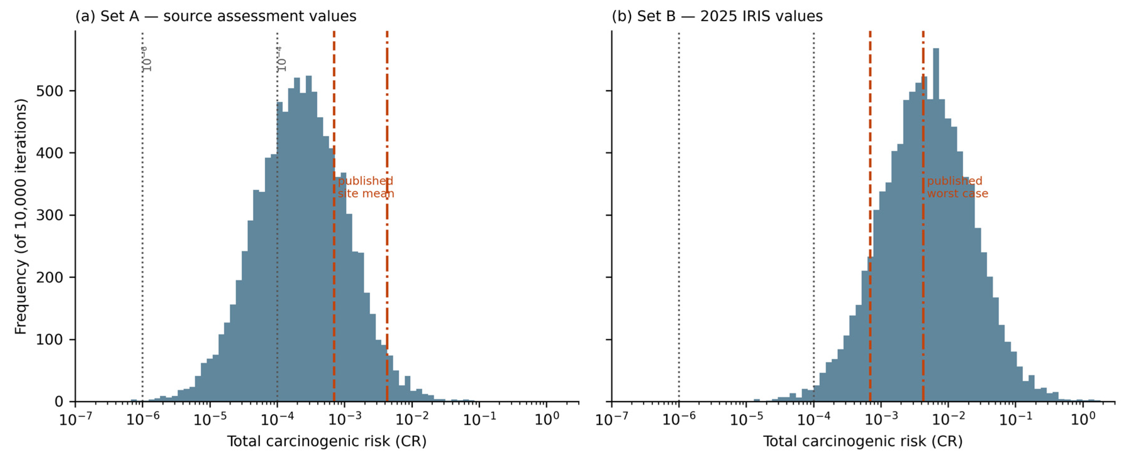
Figure 2.
Sensitivity of total carcinogenic risk to model inputs, expressed as Spearman rank correlation across 100,000 iterations. Blue denotes positive and red negative correlation. Arsenic concentration dominates (ρ = +0.867), exceeding the next-ranked input by a factor of three; inhalation rate shows negligible correlation (ρ < 0.01) under the RAGS default particulate emission factor.
Figure 2.
Sensitivity of total carcinogenic risk to model inputs, expressed as Spearman rank correlation across 100,000 iterations. Blue denotes positive and red negative correlation. Arsenic concentration dominates (ρ = +0.867), exceeding the next-ranked input by a factor of three; inhalation rate shows negligible correlation (ρ < 0.01) under the RAGS default particulate emission factor.
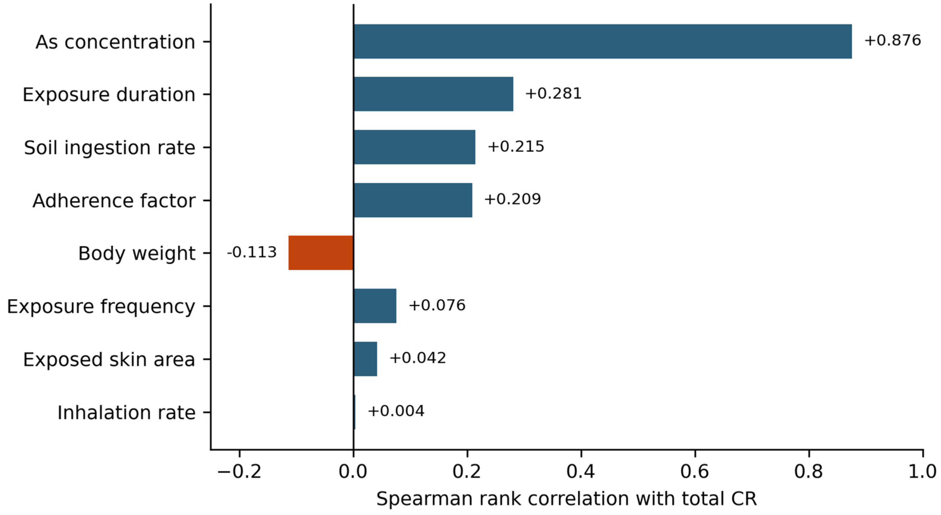
Figure 3.
Zonal comparison at the 20-year horizon under the no-intervention scenario, Set A toxicity values. Blue bars (left axis) show mean carcinogenic risk; red bars (right axis) show the probability of exceeding 10⁻⁴. Zone 2 carries the higher mean risk while Zone 1 carries the higher exceedance probability, reflecting uniformly elevated contamination within the perimeter versus spatially patchy but locally severe contamination beyond it. The Zone 2 mean is carried by two of eight samples (Table 9, Section 3.6).
Figure 3.
Zonal comparison at the 20-year horizon under the no-intervention scenario, Set A toxicity values. Blue bars (left axis) show mean carcinogenic risk; red bars (right axis) show the probability of exceeding 10⁻⁴. Zone 2 carries the higher mean risk while Zone 1 carries the higher exceedance probability, reflecting uniformly elevated contamination within the perimeter versus spatially patchy but locally severe contamination beyond it. The Zone 2 mean is carried by two of eight samples (Table 9, Section 3.6).
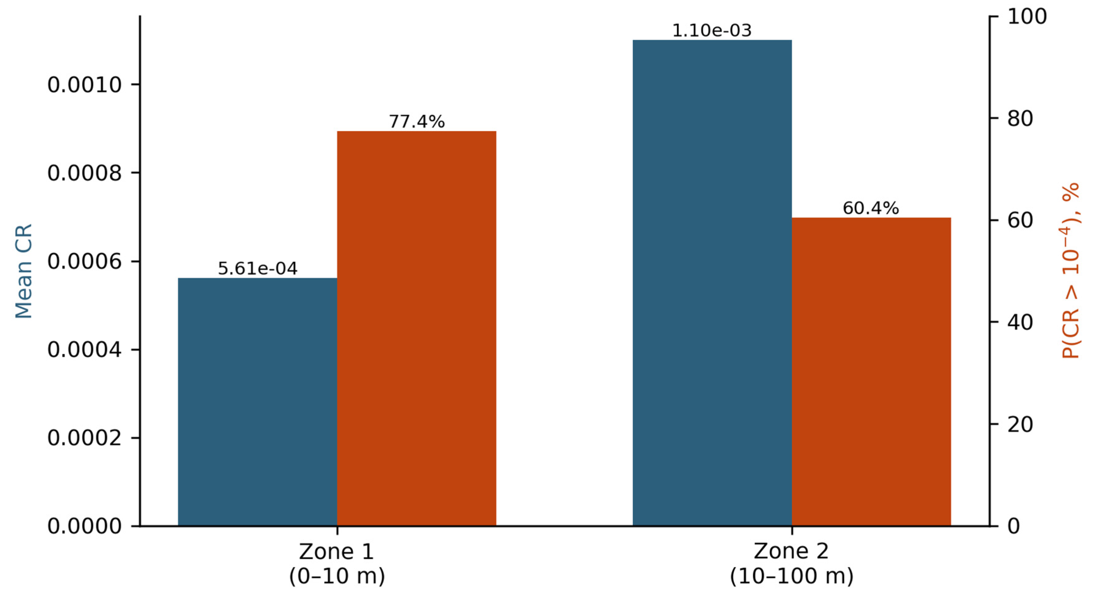
Figure 4.
Projected risk under management scenarios at 5-, 10- and 20-year horizons, Set A. (a) Mean carcinogenic risk; the dotted line marks the 10⁻⁴ threshold. (b) Probability of exceeding 10⁻⁴. S0 = no intervention; S1 = engineered containment of Zone 1 (0–10 m); S2 = containment of Zone 1 plus phytostabilization of Zone 2 (10–100 m). S1 and S2 are plotted as a single series because they differ by less than 0.3% at every horizon.
Figure 4.
Projected risk under management scenarios at 5-, 10- and 20-year horizons, Set A. (a) Mean carcinogenic risk; the dotted line marks the 10⁻⁴ threshold. (b) Probability of exceeding 10⁻⁴. S0 = no intervention; S1 = engineered containment of Zone 1 (0–10 m); S2 = containment of Zone 1 plus phytostabilization of Zone 2 (10–100 m). S1 and S2 are plotted as a single series because they differ by less than 0.3% at every horizon.
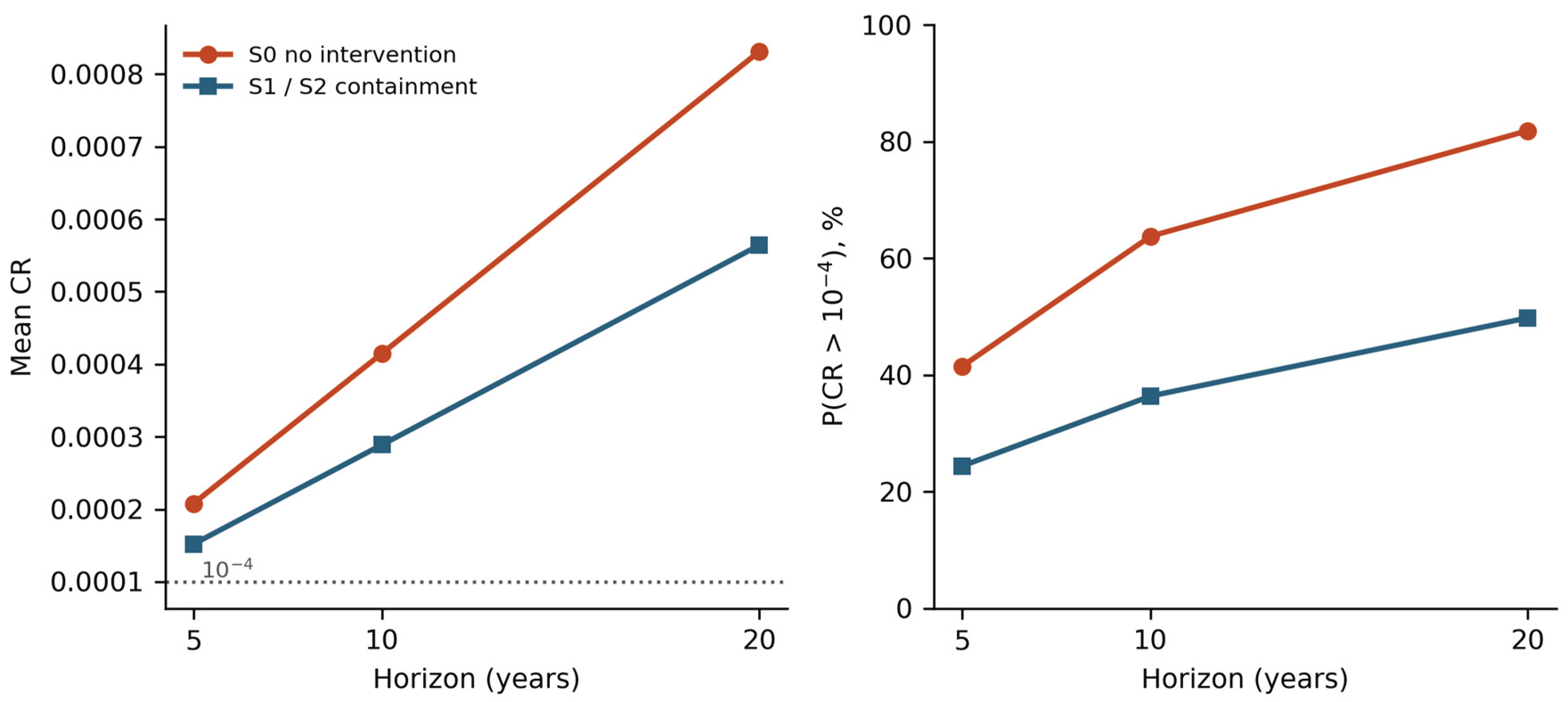

Table 1.
Fitted distribution parameters for the 24 transect samples.
| Metal | GM | GSD | AM | Min | Max | Shapiro–Wilk p (log) | Model |
| Pb | 776.9 | 3.86 | 1754 | 72.6 | 9350 | 0.339 | lognormal |
| Zn | 822.3 | 3.51 | 1254 | 7.79 | 2870 | <0.001 | empirical |
| Cd | 22.4 | 3.65 | 53.7 | 3.51 | 290 | 0.108 | lognormal |
| Cu | 405.5 | 2.68 | 684 | 80.1 | 4230 | 0.638 | lognormal |
| As | 658.2 | 3.94 | 1753 | 95.2 | 10900 | 0.176 | lognormal |
| Hg | 1.19 | 6.31 | 8.0 | 0.12 | 47.4 | <0.001 | empirical |
| Ni | 10.2 | 1.94 | 12.4 | 2.31 | 27.1 | 0.373 | lognormal |
| Cr | 6.88 | 2.22 | 9.4 | 1.79 | 36.9 | 0.955 | lognormal |
GM — geometric mean; GSD — geometric standard deviation; AM — arithmetic mean. All concentrations in mg·kg⁻¹.
Table 2.
Stochastic exposure parameters, adult outdoor-worker scenario.
| Parameter | Distribution | Parameters | Central value |
| Body weight (BW) | Normal, truncated to 40–130 | μ = 70, σ = 12 kg | 70 kg |
| Soil ingestion rate (IngR) | Lognormal | GM = 50, GSD = 2.0 mg·d⁻¹ | 50 mg·d⁻¹ |
| Inhalation rate (InhR) | Normal, truncated to 8–35 | μ = 20, σ = 3 m³·d⁻¹ | 20 m³·d⁻¹ |
| Exposed skin area (SA) | Normal, truncated to 1500–5500 | μ = 3300, σ = 660 cm² | 3300 cm² |
| Adherence factor (AF) | Lognormal | GM = 0.2, GSD = 2.0 mg·cm⁻² | 0.2 mg·cm⁻² |
| Exposure frequency (EF) | Triangular | 180 / 250 / 350 d·yr⁻¹ | 250 d·yr⁻¹ |
| Exposure duration (ED) | Triangular | 1 / 25 / 40 yr | 25 yr |
| Particulate emission factor (PEF) | Fixed | 1.36 × 10⁹ m³·kg⁻¹ | — |
| Averaging time, carcinogenic | Fixed | 70 × 365 d | — |
| Averaging time, non-carcinogenic | Fixed | ED × 365 d | — |
Table 3.
Toxicity values applied under the two parameterizations.
| Parameter (inorganic arsenic) | Set A | Set B | Basis of Set B |
| Oral slope factor, per mg·kg⁻¹·d⁻¹ | 1.5 | 32 | Combined bladder (17.6) and lung (21.3) cancer slope factors; Bayesian hierarchical dose–response meta-analysis, logistic-power model; 11 bladder and 6 lung cancer studies. Updated 13 Jan 2025 |
| Dermal slope factor, per mg·kg⁻¹·d⁻¹ | 1.5 | 32 | Oral slope factor with GI absorption = 1.0 |
| Inhalation slope factor, per mg·kg⁻¹·d⁻¹ | 15.1 | 15.1 | Derived from IUR = 4.3 × 10⁻³ per µg·m⁻³ (1995), not revised in 2025 |
| Oral RfD, mg·kg⁻¹·d⁻¹ | 3.0 × 10⁻⁴ | 6.0 × 10⁻⁵ | Endocrine and cardiovascular systems; ischemic heart disease and type 2 diabetes; UF_C = 3; confidence medium/high. Rounded from osRfDs of 5.8 × 10⁻⁵ (type 2 diabetes) and 5.7 × 10⁻⁵ (ischemic heart disease). Updated 13 Jan 2025 |
| Slope factors and RfDs, other seven metals | unchanged between sets | unchanged | IRIS |
Table 4.
Distributions of CR and HI under both parameterizations.
| Statistic | CR, Set A | CR, Set B | HI, Set A | HI, Set B |
| Mean | 7.38 × 10⁻⁴ | 1.57 × 10⁻² | 8.03 | 37.4 |
| 5th percentile | 1.78 × 10⁻⁵ | 3.63 × 10⁻⁴ | 0.439 | 1.41 |
| 25th percentile | 7.91 × 10⁻⁵ | 1.66 × 10⁻³ | 1.35 | 5.04 |
| Median | 2.26 × 10⁻⁴ | 4.77 × 10⁻³ | 3.12 | 13.0 |
| 75th percentile | 6.38 × 10⁻⁴ | 1.35 × 10⁻² | 7.58 | 34.2 |
| 95th percentile | 2.86 × 10⁻³ | 6.08 × 10⁻² | 29.2 | 141 |
| 99th percentile | 8.20 × 10⁻³ | 1.75 × 10⁻¹ | 78.3 | 386 |
| Maximum | 3.44 × 10⁻¹ | 7.34 | 3040 | 15 200 |
Table 5.
Exceedance probabilities against regulatory thresholds.
| Threshold | Set A | Set B |
| CR > 10⁻⁶ | 99.98% | 100.0% |
| CR > 10⁻⁵ | 97.8% | 100.0% |
| CR > 10⁻⁴ | 69.9% | 99.3% |
| CR > 10⁻³ | 16.8% | 84.0% |
| HI > 1 | 82.1% | 97.3% |
| HI > 4 | 42.4% | 80.1% |
| HI > 10 | 19.1% | 57.4% |
Table 6.
Position of the published point estimates within the simulated distributions.
| Published estimate | Value | Percentile, Set A | Percentile, Set B |
| Site-mean CR | 7.0 × 10⁻⁴ | 76.9 | 11.0 |
| Worst-case CR | 4.3 × 10⁻³ | 97.2 | 47.3 |
| Site-mean HI | 4.3 | 59.7 | 21.5 |
| Worst-case HI | 26.6 | 94.3 | 69.2 |
Table 7.
Sensitivity of total carcinogenic risk to model inputs (Spearman rank correlation, 100,000 iterations).
Table 7.
Sensitivity of total carcinogenic risk to model inputs (Spearman rank correlation, 100,000 iterations).
| Input | ρ |
| As concentration | +0.867 |
| Soil ingestion rate (IngR) | +0.292 |
| Exposure duration (ED) | +0.268 |
| Adherence factor (AF) | +0.133 |
| Body weight (BW) | −0.109 |
| Exposure frequency (EF) | +0.084 |
| Exposed skin area (SA) | +0.040 |
| Inhalation rate (InhR) | −0.004 |
Table 8.
Zonal risk, no-intervention scenario, 20-yr horizon.
| Zone | n | Mean As (mg·kg⁻¹) | Max As | Mean CR | P(CR > 10⁻⁴) | Mean HI |
| Zone 1 (0–10 m) | 16 | 1557 | 10 900 | 5.72 × 10⁻⁴ | 77.5% | 7.0 |
| Zone 2 (10–100 m) | 8 | 2144 | 7900 | 1.04 × 10⁻³ | 60.3% | 12.0 |
Table 9.
Leave-one-out stability of the Zone 2 : Zone 1 mean-As ratio (Zone 1 mean As = 1557 mg·kg⁻¹, n = 16; full Zone 2 ratio = 1.38).
Table 9.
Leave-one-out stability of the Zone 2 : Zone 1 mean-As ratio (Zone 1 mean As = 1557 mg·kg⁻¹, n = 16; full Zone 2 ratio = 1.38).
| Sample excluded | Transect | Distance (m) | As in sample | Zone 2 mean As | Ratio |
| 247 | South | 50 | 193 | 2423 | 1.56 |
| 248 | South | 100 | 97.6 | 2436 | 1.56 |
| 253 | North | 50 | 183 | 2424 | 1.56 |
| 254 | North | 100 | 95.2 | 2437 | 1.56 |
| 259 | East | 50 | 194 | 2423 | 1.56 |
| 260 | East | 100 | 879 | 2325 | 1.49 |
| 265 | West | 50 | 7610 | 1363 | 0.88 |
| 266 | West | 100 | 7900 | 1322 | 0.85 |
Table 10.
Scenario projections under both parameterizations.
| Set A — toxicity values of the source assessment | |||||
| T (yr) | Scenario | Mean CR | P(CR > 10⁻⁴) | ||
| 5 | S0 | 2.01 × 10⁻⁴ | 41.3% | ||
| 5 | S1 / S2 | 1.44 × 10⁻⁴ | 24.3% | ||
| 10 | S0 | 4.03 × 10⁻⁴ | 63.6% | ||
| 10 | S1 / S2 | 2.74 × 10⁻⁴ | 36.0% | ||
| 20 | S0 | 8.05 × 10⁻⁴ | 82.4% | ||
| 20 | S1 / S2 | 5.33 × 10⁻⁴ | 49.6% | ||
| Set B — 2025 IRIS values | |||||
| T (yr) | Scenario | Mean CR | P(CR > 10⁻⁴) | ||
| 5 | S0 | 4.28 × 10⁻³ | 99.1% | ||
| 5 | S1 / S2 | 3.06 × 10⁻³ | 93.6% | ||
| 10 | S0 | 8.56 × 10⁻³ | 99.9% | ||
| 10 | S1 / S2 | 5.82 × 10⁻³ | 96.4% | ||
| 20 | S0 | 1.71 × 10⁻² | 100.0% | ||
| 20 | S1 / S2 | 1.13 × 10⁻² | 98.2% | ||
Disclaimer/Publisher’s Note: The statements, opinions and data contained in all publications are solely those of the individual author(s) and contributor(s) and not of MDPI and/or the editor(s). MDPI and/or the editor(s) disclaim responsibility for any injury to people or property resulting from any ideas, methods, instructions or products referred to in the content. |
© 2026 by the authors. Licensee MDPI, Basel, Switzerland. This article is an open access article distributed under the terms and conditions of the Creative Commons Attribution (CC BY) license (http://creativecommons.org/licenses/by/4.0/).
Copyright: This open access article is published under a Creative Commons CC BY 4.0 license, which permit the free download, distribution, and reuse, provided that the author and preprint are cited in any reuse.