

Submitted:
10 September 2026
Posted:
11 September 2026
You are already at the latest version
Abstract
Conventional heart rate variability (HRV) analysis primarily characterizes R–R interval (RRI) variability, whereas the dynamic contribution structure among multiple electrocardiogram (ECG)-derived intervals and respiration remains less well understood. This study investigated the frequency-dependent organization of P–P interval (PPI), RRI, T–T interval (TTI), and respiration during postural change. Thirteen healthy young participants underwent simultaneous ECG and respiratory recording in the supine and standing positions. A four-variable multivariate autoregressive (MVAR) model was constructed, and relative power contribution (RPC) was quantified in the very-low-frequency, low-frequency (LF), and high-frequency (HF) bands and visualized as directed network topologies. Conventional HRV analysis confirmed marked autonomic modulation during standing, including shortened RRI and pronounced attenuation of HF power. RPC analysis identified 14 posture-related differences after false discovery rate correction across all 32 LF- and HF-band Source–Target comparisons. In the LF band, several TTI-related contributions increased during standing, including TTI→PPI and TTI→RRI. In the HF band, multiple PPI- and RRI-related cross-variable contributions and RRI self-contribution decreased, whereas TTI self-contribution increased markedly. Seven of the eight significant HF findings remained significant after excluding participants whose respiratory peak frequency entered the LF band. Furthermore, nine of the 14 significant RPC components remained significant across all tested P- and T-wave timing perturbations up to ±10 ms. These findings indicate that postural change reorganizes the frequency-dependent contribution structure among ECG-derived intervals and respiration. From a Network Physiology perspective, the proposed framework extends conventional RRI-centered HRV analysis by characterizing the multivariate structure and state-dependent reorganization of cardiac–respiratory dynamics.
Keywords:
heart rate variability
; ECG-derived intervals
; respiration
; multivariate autoregressive model
; network physiology
1. Introduction
In recent years, multimodal analysis integrating multiple types of measurement information has rapidly advanced in the field of biosignal analysis. In addition to physiological signals such as electrocardiogram (ECG), respiration, blood pressure, electroencephalography, and electromyography, increasing efforts have been made to combine image and text information to extract comprehensive information that cannot be obtained from a single signal alone [1,2]. Together with advances in artificial intelligence (AI) and deep learning technologies, such approaches have been widely applied to diagnostic support, disease prediction, and estimation of physiological states [3,4].
Biosignal analysis has evolved from single-modality approaches, in which signals such as ECG and electroencephalography are evaluated independently, toward multimodal approaches that integrate features extracted from multiple signals. However, in conventional multimodal analysis, each signal is often treated as an independent source of features, and oscillatory coupling and dynamic interactions among physiological subsystems are not necessarily modeled explicitly. Consequently, how multiple physiological systems interact to form integrated biological functions, and how their coupling structure changes according to physiological state, remain incompletely understood.
As a framework for addressing these issues, Network Physiology has been proposed [5], in which the human body is regarded as a network composed of multiple interacting physiological systems. Rather than treating the brain, respiratory system, cardiovascular system, and other systems as independent entities, Network Physiology views them as dynamically interacting coupled systems and characterizes their organization in terms of network structure, topology, and state-dependent changes in connectivity and interaction strength [6,7]. In the present study, this concept was applied to cardiovascular and respiratory dynamics to evaluate frequency-dependent contribution relationships among multiple physiological time series.
The present study further extends this perspective beyond relationships among different measurement modalities to the internal structure of a single modality, namely ECG. The ECG waveform is composed of multiple components, including the P wave, QRS complex, and T wave, each reflecting distinct electrophysiological processes such as atrial depolarization, ventricular depolarization, and ventricular repolarization [8]. The repeated appearance of these waveform components with each cardiac cycle forms the continuous ECG signal. Accordingly, recording ECG can also be viewed as simultaneously observing multiple beat-to-beat intervals defined by the P, R, and T waves from a single measured signal, here referred to as ECG-derived intervals.
Conventional heart rate variability (HRV) research has primarily used the R–R interval (RRI) derived from successive R waves. RRI is a representative time series of cardiac cycle duration and has been evaluated using a wide range of indices, including time-domain measures such as standard deviation of normal-to-normal intervals (SDNN) and root mean square of successive differences (RMSSD), frequency-domain measures such as low-frequency (LF) power, high-frequency (HF) power, and the LF/HF ratio [9], as well as nonlinear measures such as entropy and fractal properties [10]. These indices are widely used for the assessment of autonomic regulation, stress responses, and cardiovascular risk. In particular, a postural change from supine to standing imposes a clear regulatory demand on the cardiovascular system, and HRV analysis has been widely used to evaluate autonomic responses to orthostatic stress [11,12].
However, conventional HRV indices primarily describe the magnitude, frequency composition, and complexity of RRI variability. They do not directly evaluate how the contribution relationships among respiration and beat-to-beat intervals derived from the P, R, and T waves change with postural transition.
One reason RRI has been used so extensively is that the QRS complex, particularly its prominent R wave, can generally be detected more reliably than the lower-amplitude P and T waves, and QRS detection has been widely applied in continuous and long-term ECG monitoring [13]. In contrast, P and T waves are generally more difficult to detect than the prominent QRS complex, particularly because lower-amplitude components such as the P wave are more susceptible to noise and morphological variability [14]. Respiratory measurement may also require an additional sensor placed on the chest or abdomen, imposing an additional burden under real-world recording conditions. Because of these acquisition and analytical challenges, multivariate analyses including the P–P interval (PPI), T–T interval (TTI), and respiration have been less extensively investigated than analyses based on RRI alone.
It is well established that HRV is strongly influenced by respiration. Respiratory sinus arrhythmia (RSA) is a representative phenomenon in which respiratory rhythm induces periodic modulation of RRI through autonomic regulation [15]. Many previous studies have focused primarily on the relationship between RRI (or heart period) and respiration, including bivariate analyses of cardiorespiratory coupling [16,17], whereas multivariate contribution structures incorporating PPI and TTI have received considerably less attention. Consequently, the frequency-dependent dynamic relationships among PPI, RRI, TTI, and respiration remain insufficiently characterized.
PPI, TTI, and respiration are more difficult to acquire or analyze than RRI but may contain additional information relevant to understanding the structure of cardiac and respiratory dynamics. Incorporating these variables into the analysis makes it possible to examine how their fluctuations are related to RRI and to one another. Univariate HRV analysis can characterize the properties of RRI variability in detail; however, it cannot simultaneously decompose RRI variability into contributions attributable to its own past dynamics and to the past dynamics of respiration and other ECG-derived intervals.
To use such information for physiological analysis, a methodological basis is required for reliably extracting P-, R-, and T-wave peaks and constructing stable time series from the temporal information derived from these fiducial points. We have previously developed an analytical environment that allows users to locally correct residual R-peak detection errors through a graphical user interface (GUI) while visually inspecting the ECG waveform after automatic detection, with immediate updating of RRI and related analytical results [18]. We have also proposed a method that combines lightweight binary classifiers with physiological temporal constraints (PTC) to reduce false-positive detections of P, R, and T waves [19]. These previous studies provide a methodological basis for reliably extracting ECG peaks and utilizing ECG-derived intervals for physiological analysis.
In the present study, we constructed a four-variable multivariate autoregressive (MVAR) model consisting of PPI, RRI, TTI, and respiration and quantified frequency-dependent contribution relationships among these time series by calculating relative power contribution (RPC) in the frequency domain [20,21,22]. This approach evaluates, within each frequency band, the relative extent to which fluctuations in each variable are associated with their own past dynamics and with the past dynamics of the other variables. Thus, rather than treating HRV as a single RRI time series, the present framework describes cardiac and respiratory variability as a multivariate coupled oscillatory system composed of ECG-derived intervals and respiration.
The first aim of this study was to present an analytical framework for visualizing the cardiac–respiratory variability network composed of PPI, RRI, TTI, and respiration as a frequency-specific contribution topology and for evaluating it from the perspective of Network Physiology. The second aim was to determine how the contribution structure among these time series changes across frequency bands during the transition from supine to standing. Through these analyses, we examined whether ECG-derived intervals, which have been less extensively investigated because of acquisition and analytical difficulties, contain physiological information relevant to understanding the coordinated structure of cardiac and respiratory variability and its posture-dependent reorganization.
2. Materials and Methods
2.1. Participants and Experimental Protocol
Thirteen healthy students participated in this study (age: 23 ± 2 years; 3 women and 10 men). The inclusion criteria were healthy students aged 18 years or older who had received an explanation of the purpose and procedures of the study and voluntarily agreed to participate. All participants were provided with a detailed explanation of the experimental procedures and study content before participation, and written informed consent was obtained prior to the experiment.
The exclusion criteria were as follows: (i) persistent atrial fibrillation or frequent premature beats, (ii) the presence of a serious medical condition, or (iii) a determination by the principal investigator that participation was inappropriate. Eligibility with respect to the exclusion criteria was confirmed before measurement on the basis of self-reported information obtained during a pre-experimental interview. In addition, the ECG waveform was visually inspected by the investigator before recording, and the measurement was to be discontinued if an obvious irregular cardiac rhythm was observed.
Two postural conditions, supine and standing, were adopted in the experimental protocol to induce different states of autonomic regulation while allowing stable recording of ECG and respiratory signals. First, participants rested in the supine position. After confirming that the ECG waveform was stable, ECG and respiration were recorded simultaneously for 7 min while the participants remained awake with their eyes open. Participants then stood up by themselves and remained at rest in the upright standing position. After confirming that the ECG waveform had stabilized, ECG and respiration were again recorded simultaneously for 7 min. For each postural condition, the 6-min period from 1 to 7 min after the start of recording was used for analysis to exclude transient effects immediately following the postural transition. Participants breathed spontaneously throughout the experiment and were instructed not to intentionally take deep breaths. No participant coughed during the recordings.
ECG was recorded using a Polymate Pro MP6000 biosignal recording system (Miyuki Giken Co., Ltd., Tokyo, Japan). A three-electrode configuration was used, with the right wrist as the reference electrode, the left ankle as the recording electrode, and the left wrist as the ground electrode, yielding an ECG signal equivalent to Lead II. Respiration was recorded using an AP-C034-013(S) air-pressure DC respiratory sensor and an AP-U033 respiratory adapter (Miyuki Giken Co., Ltd., Tokyo, Japan). The respiratory sensor was positioned around the thoracoabdominal region at the level of the epigastrium.
Pressure changes associated with respiratory movements were converted into voltage signals by a strain-gauge pressure transducer within the adapter (Figure 1). ECG and respiratory signals were synchronously recorded using the same biosignal acquisition system, and both signals were sampled at 500 Hz.
2.2. Biosignal Preprocessing
P-, R-, and T-wave peaks were detected from the ECG using the PTC-based peak detection framework described previously [19]. In this framework, R-wave peaks were detected first and subsequently used as temporal landmarks for P- and T-wave peak detection within physiologically plausible pre- and post-R time windows. When missed or false peak detections were identified, peaks were added, deleted, or repositioned while visually inspecting the ECG waveform using a previously developed prototype GUI [18].
The peak times of consecutively detected P, R, and T waves were denoted as , , and , respectively. The PPI, RRI, and TTI were calculated from the time differences between successive peaks of the same type as follows:
Because each interval becomes fully defined only when the later peak forming that interval occurs, each interval value was assigned to the time of the later peak. Accordingly, the time associated with each interval series was defined as follows:
This assignment ensures that, at each timestamp, the interval represents a completed cardiac interval rather than one that will be completed in the future. This temporal definition is consistent with autoregressive (AR) modeling, in which the current state is modeled as a function of past observations. Consequently, even when PPI, RRI, and TTI corresponded to the same sequence of cardiac cycles, they were located at different positions on the real-time axis because they were referenced to different ECG fiducial points (Table 1).
To align the input times for the four-variable MVAR model, a common real-time grid with an interval of 0.5 s (2 Hz) was established over the analysis segment. PPI, RRI, and TTI were resampled onto this common time grid using piecewise cubic spline interpolation while preserving the real-time assignments originally associated with each interval series. The respiratory signal was also resampled onto the same real-time grid. This procedure produced a four-variable time series in which PPI, RRI, TTI, and respiration at each time point corresponded to the same real time (Table 2).
To eliminate differences in amplitude scale among variables, each time series was standardized to a mean of 0 and a standard deviation (SD) of 1. Subsequently, a 0.03-Hz high-pass filter was applied to each time series to suppress very-low-frequency (VLF) drift and nonstationary components and to improve the stability of MVAR estimation.
2.3. MVAR Modeling and RPC Analysis
2.3.1. RPC Analysis Using an MVAR Model
In this study, an MVAR model was used to evaluate frequency-dependent relationships among the four time series of PPI, RRI, TTI, and Resp. An MVAR model describes the dynamic dependency structure among multiple time series by expressing the current value of each series as a linear combination of its own past values and the past values of the other series. By transforming the estimated MVAR coefficients into the frequency domain, the power contribution from each Source to each Target can be calculated at each frequency [20,21,22].
The four-variable time-series vector was defined as
where the superscript T denotes the transpose. An MVAR model of order p was expressed as
where is the MVAR coefficient matrix at lag k, and is the innovation vector. The innovation vector was defined as
and represents new fluctuations in each series that cannot be explained by the past information included in the model.
2.3.2. Selection of MVAR Model Order
The maximum order of the MVAR model was set to 40. The Akaike information criterion (AIC), Bayesian information criterion (BIC), Hannan–Quinn information criterion (HQIC), and final prediction error (FPE) were calculated. In the present study, the order selected by FPE was used as the first candidate. If the FPE-selected model did not satisfy the stability criterion, the model order was reduced one order at a time, and the first model satisfying the stability criterion was adopted as the final model.
Because the sampling frequency of the time series used for analysis was 2 Hz, the maximum order of 40 samples corresponded to 20 s. The model order was selected separately for each participant and each postural condition.
2.3.3. Frequency-Domain Transformation and Calculation of Component Power
The estimated MVAR model was transformed into the frequency domain. The polynomial matrix at frequency f was defined as
where I is the identity matrix, fs is the sampling frequency, and j is the imaginary unit.
The transfer function matrix was obtained as
The component power at frequency f in Target i attributable to the innovation of Source j was defined as
where is the transfer-function component from Source j to Target i, and is the diagonal element of the innovation covariance matrix Σ corresponding to Source j [20,21,22].
For visualization of the frequency-dependent RPC ratios, the component powers were normalized across the four Sources at each frequency for each Target as
such that at each frequency.
When Source and Target were identical, the component was treated as a self-contribution. Accordingly, four contributions, with PPI, RRI, TTI, and Resp as Sources, were calculated for each Target. For example, when RRI was the Target, the four components PPI→RRI, RRI→RRI, TTI→RRI, and Resp→RRI were calculated, with RRI→RRI defined as the RRI self-contribution.
The analysis segment for each postural condition was 360 s, corresponding to a basic frequency interval of
Based on this interval, the frequency responses of the MVAR model and the RPC values were calculated on a frequency grid with a spacing of 0.003 Hz.
2.3.4. Band-Specific RPC
The frequency bands were defined as VLF (0.003–0.04 Hz), LF (0.04–0.15 Hz), and HF (0.15–0.50 Hz). For each Source–Target component, the component power within frequency band was integrated over frequency using the trapezoidal rule:
where represents the integrated component power from Source j to Target i within frequency band b.
The band-specific RPC was normalized using the sum of the 12 components obtained for each Target, consisting of four Sources across three frequency bands:
where represents the normalized RPC from Source j to Target i within frequency band b.
This normalization satisfies
for each participant, each postural condition, and each Target.
Separate normalization within each frequency band was not performed, thereby preserving the relative contributions across the VLF, LF, and HF bands. This allowed relative changes in the same Source–Target–Band component to be compared between the supine and standing conditions.
The primary analyses focused on RPC values in the LF and HF bands. The upper limit of the HF band was set to 0.50 Hz to retain respiratory components in the HF range because respiration was explicitly included in the MVAR model. Because the 0.03-Hz high-pass filter attenuated the lower portion of the VLF range, VLF components were retained as part of the global normalization but were not included in the primary posture comparisons.
2.3.5. Topological Visualization of RPC Networks
In Network Physiology, interactions among physiological systems can be represented as network links, and their organization can be characterized in terms of network structure, topology, and link strength [5,6,7]. In the present study, we introduced a directed RPC network representation to visualize the frequency-dependent contribution structure among PPI, RRI, TTI, and Resp. The four variables were represented as nodes, with PPI on the left, RRI at the top, TTI on the right, and Resp at the bottom. For each Source–
Target pair, the mean band-specific RPC across participants was represented by a directed arrow from Source to Target, whereas self-contributions were represented by self-loops. Arrow width and color were scaled according to the magnitude of the mean RPC.
Separate RPC network topologies were constructed for the LF and HF bands and for the supine and standing conditions. Components showing significant posture-related differences after Benjamini–Hochberg false discovery rate (FDR) correction were marked with asterisks in the standing topology.
2.4. Statistical Analysis
2.4.1. Descriptive Statistics and Conventional HRV Analysis
For the PPI, RRI, and TTI time series, the mean, SD, 95% confidence interval (CI), skewness, and kurtosis were calculated. For the respiratory signal, a 0.03-Hz high-pass filter was applied, the power spectral density was estimated using Welch’s method, and the dominant peak frequency within 0.05–0.50 Hz was identified.
Conventional HRV analysis was performed using the unstandardized RRI time series. Mean RRI (ms) was calculated before high-pass filtering. For spectral analysis, the RRI time series was high-pass filtered at 0.03 Hz and mean-centered, and the power spectral density (ms²/Hz) was estimated using a univariate AR model. The AR model order was selected within a maximum order of 40 on the basis of the FPE. From the estimated power spectrum, LF power (0.04–0.15 Hz, ms²), HF power (0.15–0.40 Hz, ms²), and the LF/HF ratio (dimensionless) were calculated.
For conventional HRV analysis, the HF band was defined as 0.15–0.40 Hz, whereas the HF band for MVAR-based RPC analysis was defined as 0.15–0.50 Hz to retain respiratory components in the HF range.
2.4.2. Normality Assessment and Posture Comparison
Before comparing the supine and standing conditions, the normality of the within-participant difference (Standing − Supine) was assessed for each variable using the Shapiro–Wilk test. When the distribution of the paired differences did not significantly deviate from normality, a paired -test was used. When normality was not satisfied, the Wilcoxon signed-rank test was applied.
This procedure was used for comparisons of mean RRI, LF power, HF power, LF/HF, and respiratory peak frequency.
2.4.3. Multiple-Comparison Correction and Effect Size
For the RPC analysis, the within-participant difference (Standing − Supine) was calculated for each Target, frequency band, and Source–Target component. Before each paired comparison, the normality of the paired differences was assessed using the Shapiro–Wilk test. When the paired differences did not significantly deviate from normality, a paired t-test was used; otherwise, the Wilcoxon signed-rank test was applied to compare the supine and standing conditions.
The RPC analysis included PPI, RRI, TTI, and Resp as four Targets. For each Target, four Source components corresponding to PPI, RRI, TTI, and Resp were evaluated in the LF and HF bands, resulting in a total of 32 Source–Target–Band comparisons. When the Source and Target were identical, the component was treated as a self-contribution. To control for multiple comparisons, the Benjamini–Hochberg procedure was applied jointly across all 32 LF- and HF-band Source–Target comparisons. An FDR-adjusted p-value of <0.05 was considered statistically significant.
Cohen’s dz was calculated as the effect size for all paired comparisons, irrespective of the statistical test selected. Cohen’s dz was calculated as
where is the mean within-participant difference (Standing − Supine), and SDD is the SD of the paired differences. A positive dz indicates an increase during standing, whereas a negative dz indicates a decrease during standing.
As a sensitivity analysis, the RPC comparisons were repeated after excluding participants whose respiratory peak frequency fell within the LF band in either posture (sub4, sub7, and sub11), resulting in n=10. The same statistical procedure and FDR correction as in the main analysis were applied.
2.4.4. Residual Diagnostics
To evaluate the residual characteristics of the MVAR models, the Ljung–Box test was applied to the residual time series of each variable. In addition, a multivariate Portmanteau test was performed to assess the multivariate residual whiteness of each MVAR model. The number of lags used for the multivariate residual whiteness test was set to twice the final MVAR model order, and a small-sample correction was applied.
These residual whiteness tests were performed for model diagnostic purposes and were not used as exclusion criteria for the analysis.
A two-sided p<0.05 was considered statistically significant. All analyses were performed using Python 3.12.7 (64-bit), primarily with NumPy, pandas, SciPy, and statsmodels.
2.5. Robustness Analysis for P- and T-Wave Timing Jitter
2.5.1. Generation of P- and T-Wave Timing Jitter
To evaluate the influence of small temporal errors that may occur in P- and T-wave peak localization on the MVAR-derived RPC results, a robustness analysis was performed by introducing timing jitter. Jitter was applied separately to P- and T-wave peaks. R-wave peak times were left unchanged.
For each P- or T-wave peak, the original sample position was denoted by , and an integer-valued random shift was selected from a discrete uniform distribution over
s ∈ {−J, −J+1, …0, …, J −1, J }
The jittered peak position was then defined as
n′= n+s
Because the ECG sampling frequency was 500 Hz, one sample corresponded to 2 ms. In the present study, J =1, 2, 3, 4, and 5 samples were used, corresponding to maximum timing deviations of ±2, ±4, ±6, ±8, and ±10 ms, respectively. For example, under the ±4-ms condition, a temporal shift of −4, −2, 0, +2, or +4 ms was randomly assigned to each peak. The condition without added jitter was defined as the jitter-off condition.
For each participant, postural condition, and jitter amplitude, one random jitter realization was generated. If a jittered peak position overlapped an existing peak position, the original peak position was retained to prevent a change in the number of detected peaks. If the shifted peak position fell outside the analysis range, it was adjusted to remain within the analysis range.
2.5.2. Reconstruction of Interval Time Series and MVAR/RPC Reanalysis
For P-wave timing jitter, the PPI time series was recalculated from the jittered P-wave peak times. For T-wave timing jitter, the TTI time series was recalculated from the jittered T-wave peak times. R-wave peak times and the respiratory signal were left unchanged.
For each jitter condition, the same preprocessing and MVAR/RPC analysis procedures described in Section 2.2 and Section 2.3 were applied to the four time series containing the reconstructed PPI or TTI. The MVAR model order was not fixed to that obtained under the jitter-off condition; instead, it was independently reselected for each participant, postural condition, and jitter amplitude.
2.5.3. Assessment of Robustness of Posture-Related RPC Changes
For each P-wave and T-wave timing-jitter condition, RPC values were calculated in the LF and HF bands. The same statistical procedures described in Section 2.4.3 were applied to comparisons between the supine and standing conditions.
Robustness to timing jitter was evaluated by determining whether the posture-related RPC changes observed under the jitter-off condition were preserved when random temporal perturbations of up to ±10 ms were introduced into the P- or T-wave peak times.
3. Results
3.1. Detection of P-, R-, and T-wave Peaks and Derived Interval Time Series
Figure 2 shows a representative example of P-, R-, and T-wave peak detection during the first 30 s of the analyzed segment in the supine and standing conditions. P-, R-, and T-wave peaks were continuously identified in both postures. Representative videos showing the visual confirmation of P-, R-, and T-wave peak detection by sequentially reviewing the detected ECG waveforms are provided as Supplementary Videos S2–S4, respectively. These videos show ECG data from subject 1 in the standing condition.
Figure 3 shows the PPI, RRI, TTI, and respiratory time series derived from the same representative participant over the entire 360-s analysis segment. PPI, RRI, and TTI exhibited similar beat-to-beat temporal variations within each posture. The interval series showed lower values during standing than during the supine condition in this participant. The respiratory signal exhibited continuous respiratory oscillations superimposed on a gradual baseline drift over the analysis segment. These time series are presented before application of the 0.03-Hz high-pass filter used for the MVAR analysis.
3.2. Descriptive Characteristics of PPI, RRI, TTI, and Respiration
Individual descriptive characteristics of PPI, RRI, TTI, and respiratory peak frequency are summarized in Table 3. Across the 13 participants, mean PPI, RRI, and TTI values were lower during standing than during the supine condition. Within each participant and posture, the mean values of PPI, RRI, and TTI were closely similar, with slight differences in temporal variability among the three interval series.
Respiratory peak frequency varied among participants and between postures. Respiratory peak frequency ranged from 0.134 to 0.339 Hz in the supine condition and from 0.125 to 0.383 Hz in the standing condition. The direction of the posture-related change in respiratory peak frequency was not uniform across participants.
3.3. MVAR Model Order and Residual Diagnostics
Table 4 summarizes the selected MVAR model orders and residual diagnostic results for each participant and posture. The model orders selected by AIC, BIC, HQIC, and FPE for each participant and posture are provided in Table S1.
The selected MVAR model order varied among participants and between postures. In the supine condition, the final model order ranged from 5 to 14, with a mean of 9.6 ± 2.5 and a median of 10, corresponding to a mean temporal span of approximately 4.8 s at the 2-Hz sampling rate. In the standing condition, the final model order ranged from 6 to 16, with a mean of 9.9 ± 2.7 and a median of 9, corresponding to a mean temporal span of approximately 5.0 s. The final model order differed between postures in 12 of the 13 participants.
In 23 of the 26 participant–posture models, the order selected by FPE was adopted as the final model order. In three supine-condition models (sub5, sub9, and sub11), the FPE-selected order was reduced according to the predefined stability criterion, resulting in final orders of 7, 8, and 5, respectively.
Multivariate residual whiteness was satisfied at the 0.05 level in 3 of the 26 models (sub8 in both postures and sub13 in the supine condition). As specified in the Methods, residual whiteness was evaluated as a model diagnostic and was not used as an exclusion criterion.
3.4. Conventional HRV Analysis
Table 5 summarizes the conventional HRV indices and respiratory peak frequency in the supine and standing conditions. Mean RRI was significantly lower during standing than during the supine condition (945 ± 170 vs. 720 ± 113 ms, p<0.001, Cohen’s dz = −2.73).
LF power was also significantly lower during standing (median [interquartile range (IQR)], 463 [1730] vs. 437 [477] ms², p=0.048, Cohen’s dz = −0.59). HF power showed a marked reduction during standing (1061 [3545] vs. 147 [166] ms², p<0.001, Cohen’s dz = −0.92), whereas the LF/HF ratio was significantly higher (0.783 [0.655] vs. 3.093 [4.162], p<0.001, Cohen’s dz =1.21).
Respiratory peak frequency did not differ significantly between postures (0.232 ± 0.068 vs. 0.223 ± 0.078 Hz, p=0.71, Cohen’s dz = −0.11).
3.5. Frequency-Specific RPC
Figure 4 and Figure 5 show the frequency-dependent component power and RPC ratios for Sub1 during the supine and standing conditions, respectively. The left panels show the component-power spectra for each target variable, and the right panels show the corresponding frequency-dependent RPC ratios.
During the supine condition (Figure 4), the measured respiratory peak frequency was 0.337 Hz. In the RRI target, component-power peaks were observed around 0.1 Hz and near the respiratory peak frequency. Around 0.337 Hz, the relative contribution from respiration increased, whereas the lower-frequency component around 0.1 Hz showed larger contributions from the ECG-derived interval variables. In the respiratory target, the total component power showed peaks around 0.1 Hz and near 0.337 Hz. The respiratory self-component was largest near the respiratory peak frequency, whereas the lower-frequency component contained larger contributions from PPI and RRI.
During the standing condition (Figure 5), the measured respiratory peak frequency was 0.156 Hz. In the RRI target, a prominent component-power peak was observed around 0.1 Hz, with another component near the respiratory peak frequency. The LF component showed a large contribution from TTI, whereas the respiratory contribution increased around 0.15–0.18 Hz. In the respiratory target, a prominent peak was observed near 0.156 Hz, where the respiratory self-component was also large.
The TTI target also showed a marked difference between postures. During standing, the TTI self-component accounted for most of the RPC over a broad frequency range, whereas the contributions from PPI, RRI, and respiration were smaller. In the PPI target, respiration-related contributions were also observed around the respiratory-frequency region during both postures.
3.6. Statistical Comparison of RPC between Supine and Standing.
Significant posture-related differences in RPC were observed in 14 of the 32 Source–Target–Band components after Benjamini–Hochberg FDR correction across all 32 LF- and HF-band comparisons (Table 6). In the LF band, TTI→PPI, PPI→RRI, RRI self, TTI→RRI, TTI self, and TTI→Resp were significantly greater during standing than during the supine condition. In the HF band, RRI→PPI, PPI→RRI, RRI self, PPI→TTI, RRI→TTI, PPI→Resp, and RRI→Resp were significantly lower during standing, whereas TTI self was significantly greater during standing.
The sensitivity analysis excluding three participants (sub4, sub7, and sub11) whose respiratory peak frequencies fell within the LF band yielded a broadly similar pattern. Seven of the eight HF components that were significant in the main analysis remained significant in the n=10 sensitivity analysis; PPI→RRI no longer reached FDR-adjusted significance (pFDR = 0.057). In the LF band, TTI→PPI, RRI self, and TTI→RRI remained significant, whereas PPI→RRI, TTI self, and TTI→Resp no longer reached FDR-adjusted significance.
Taken together, the main analysis showed increases in several LF components during standing, while the HF band was characterized predominantly by decreases in cross-variable contributions and an increase in the TTI self-component. Most HF findings remained significant in the sensitivity analysis, whereas several LF findings were attenuated after exclusion of participants with LF-range respiratory peak frequencies.
3.7. Topological Representation of RPC Networks
Figure 6 shows the mean RPC topologies in the supine and standing conditions for the LF and HF bands for the 13 participants in the main analysis. The top panels represent the supine condition, and the bottom panels represent the standing condition. Asterisks indicate Source–Target components that showed significant differences between the two postures after Benjamini–Hochberg FDR correction across all 32 LF- and HF-band comparisons.
In the LF band, the standing topology showed increased contributions from TTI to PPI, PPI to RRI, and TTI to RRI, together with increases in the RRI self-contribution, TTI self-contribution, and TTI→Resp contribution. By contrast, most other LF components remained visually similar between postures.
In the HF band, the standing topology showed reduced contributions from RRI to PPI, PPI to RRI, PPI to TTI, RRI to TTI, PPI to Resp, and RRI to Resp, whereas the TTI self-contribution remained markedly increased. The RRI self-contribution was also reduced in the standing condition. The HF topology in standing was characterized by attenuation of several inter-variable couplings together with strengthening of the TTI self-component.
3.8. Robustness to P- and T-Wave Timing Jitter
The robustness of posture-related RPC differences was evaluated by independently introducing P- or T-wave timing jitter ranging from ±2 to ±10 ms (Table 7). Among the 14 RPC components that were significant in the jitter-off condition, nine remained significant after Benjamini–Hochberg FDR correction across all 32 LF- and HF-band comparisons under every P-wave and T-wave jitter condition.
In the LF band, TTI→PPI and TTI→RRI remained significant across all jitter conditions. PPI→RRI and the RRI self-contribution were no longer significant under any P-wave or T-wave jitter condition. The TTI self-contribution remained significant up to ±6 ms of P-wave jitter but not at ±8 or ±10 ms, and it was not significant under any T-wave jitter condition. TTI→Resp remained significant across all P-wave jitter conditions; under T-wave jitter, significance was retained up to ±6 ms but not at ±8 or ±10 ms.
In the HF band, seven of the eight components that were significant in the jitter-off condition remained significant across all P-wave and T-wave jitter conditions: RRI→PPI, RRI self-contribution, PPI→TTI, RRI→TTI, TTI self-contribution, PPI→Resp, and RRI→Resp. PPI→RRI remained significant across all P-wave jitter conditions and up to ±6 ms of T-wave jitter, but was no longer significant at ±8 or ±10 ms of T-wave jitter.
The direction of Cohen’s dz was preserved across all jitter conditions for the RPC components that were significant in the jitter-off analysis.
4. Discussion
The present study applied a four-variable MVAR framework to PPI, RRI, TTI, and respiration and visualized their frequency-specific RPC patterns as directed topologies. The main findings were that posture-related changes were frequency dependent and involved both cross-variable and self-contributions. In the LF band, several TTI-related contributions increased during standing, including TTI→PPI and TTI→RRI. In the HF band, several cross-variable contributions involving PPI and RRI decreased, whereas the TTI self-contribution increased markedly. Most of these HF findings remained significant in the sensitivity analysis excluding participants with LF-range respiratory peak frequencies. In addition, nine of the 14 posture-related RPC differences observed in the jitter-off condition remained significant across all tested P- and T-wave timing jitter levels.
4.1. Conventional HRV and Posture-Related Autonomic Modulation
Conventional HRV analysis confirmed clear posture-related changes in cardiac autonomic modulation. Mean RRI decreased markedly from the supine to the standing condition, indicating the expected increase in heart rate during orthostatic stress. HF power also decreased substantially during standing, whereas the LF/HF ratio increased. These findings are consistent with the well-established autonomic response to standing, which involves cardiac vagal withdrawal together with increased sympathetic activation [11,12]. Orthostatic challenge has been shown to reduce vagally mediated HRV indices and shorten the RRI, while head-up tilt studies have similarly demonstrated progressive reductions in HF power with increasing tilt angle.
LF power was also significantly lower during standing than in the supine condition in the present study. This finding should not necessarily be interpreted as evidence of reduced sympathetic activity, because absolute LF power is not a specific measure of cardiac sympathetic modulation. Previous work has shown that the LF component of HRV reflects contributions from both sympathetic and parasympathetic mechanisms, and the interpretation of LF power and the LF/HF ratio as direct measures of sympathetic tone or sympathovagal balance remains controversial [23]. Accordingly, the conventional HRV findings in the present study are best interpreted as demonstrating a marked reorganization of autonomic cardiac regulation during standing, characterized particularly by heart-rate acceleration and pronounced attenuation of HF variability.
Respiratory peak frequency did not differ significantly between the supine and standing conditions. The marked reduction in HF power observed during standing cannot be attributed simply to a systematic group-level shift in respiratory frequency. This is important for the subsequent RPC analysis because respiratory dynamics were explicitly included as one of the four variables in the MVAR model.
In three participants, the dominant respiratory frequency fell within the conventional LF band in at least one posture (sub4 during standing, sub7 during supine, and sub11 during standing). When respiratory frequency shifts into the LF range, RSA can contribute directly to LF power [24,25]. A large LF component during the supine condition may reflect vagally mediated respiratory oscillations rather than enhanced sympathetic modulation. During standing, HF power is generally attenuated with vagal withdrawal, while LF power may be augmented when the respiratory oscillation itself falls within the LF band. Therefore, LF power cannot be interpreted solely as an index of sympathetic modulation, particularly in participants with LF-range respiration.
4.2. Frequency-Dependent Reorganization of the RPC Topology
The present RPC analysis demonstrated that the posture-related reorganization of the multivariate contribution structure differed substantially between the LF and HF bands. In the LF band, TTI→PPI, PPI→RRI, RRI self-contribution, TTI→RRI, TTI self-contribution, and TTI→Resp were significantly greater during standing than during the supine condition.
However, after excluding the three participants whose respiratory peak frequency fell within the LF band in at least one posture, only TTI→PPI, RRI self-contribution, and TTI→RRI remained significant. In the restricted n=10 analysis, PPI→RRI, TTI self-contribution, and TTI→Resp no longer reached FDR-adjusted significance. Because this sensitivity analysis both excluded participants with LF-range respiration and reduced the sample size, the loss of significance in these LF components cannot be attributed solely to respiratory frequency.
In contrast, the HF-band topology showed a broader and more consistent reorganization during standing. The contributions of RRI→PPI, PPI→RRI, PPI→TTI, RRI→TTI, PPI→Resp, and RRI→Resp were significantly reduced, together with a reduction in RRI self-contribution. The TTI self-contribution increased markedly during standing. Importantly, seven of the eight HF components that showed significant posture-related differences in the main analysis remained significant after exclusion of the three participants with LF-range respiration; only PPI→RRI no longer reached FDR-adjusted significance (pFDR = 0.057). This indicates that most of the observed HF topology was preserved in the sensitivity analysis.
The widespread reduction in PPI- and RRI-related HF contributions is consistent with the pronounced attenuation of conventional HF power observed during standing. Because respiratory-frequency heart-period oscillations are strongly modulated by cardiac vagal activity [15], vagal withdrawal during orthostatic stress may reduce the extent to which respiratory-frequency fluctuations are shared among the ECG-derived interval series. In the present MVAR representation, this change was expressed not only as reduced conventional RRI HF power, but also as a redistribution of HF-band relative contributions among PPI, RRI, TTI, and respiration. The reduction in RRI self-contribution indicates that the HF-band dynamics of RRI became less dominated by its own past dynamics during standing.
Importantly, the increases observed in selected LF RPC components represent changes in relative contribution rather than increases in absolute LF power. In the present analysis, RPC was normalized for each target across all four sources and the VLF, LF, and HF bands, such that the sum of the 12 Source × Band components was equal to unity. Consequently, a reduction in HF contributions necessarily increases the relative share allocated to the remaining LF and/or VLF components, even if their absolute component power does not increase. Absolute LF power also decreased during standing, but the reduction in HF power was substantially greater, resulting in a marked increase in the LF/HF ratio. This shift in the relative balance between LF and HF power may partly account for the increased relative representation of selected LF components in the normalized RPC topology. The LF findings indicate a redistribution of the relative contribution structure toward selected LF components rather than a generalized enhancement of LF oscillatory power.
Taken together, these findings indicate that orthostatic stress did not produce a uniform change across frequency bands. Such state-dependent reorganization of interaction patterns is consistent with the Network Physiology concept that physiological transitions can be accompanied by changes in network topology and link organization [5,6,7]. The HF band was characterized by widespread reductions in PPI- and RRI-related contributions together with a marked increase in TTI self-contribution, whereas the LF band showed a more selective redistribution toward particular components. Notably, two of the three LF components that remained significant in the sensitivity analysis originated from TTI (TTI→PPI and TTI→RRI). This persistence indicates that TTI-related dynamics contributed to the posture-dependent reorganization even after participants with LF-range respiration were excluded. This possibility is considered in the following section in relation to ventricular repolarization dynamics.
Despite marked posture-dependent reorganization of the RPC topology, the temporal horizon represented by the fitted MVAR models was approximately 5 s in both postures, suggesting that the short-term timescale captured by the models remained broadly similar across postural states.
4.3. TTI–RRI Contributions and Ventricular Repolarization-Related Dynamics
A notable finding of the present study was the posture-related increase in TTI-related contributions, particularly the increase in TTI→RRI in the LF band and the marked increase in TTI self-contribution in the HF band. These findings suggest that temporal dynamics associated with T-wave timing became more prominent within the multivariate ECG-derived interval network during standing. Because TTI is defined from successive T-wave peaks, it contains not only information related to the cardiac cycle length but also beat-to-beat changes in the timing of the T wave relative to the R wave. The relationship between TTI and RRI can be expressed directly from their definitions:
where RTn = Tn − Rn denotes the R-to-T-peak interval of beat n.
TTIn−RRIn = (Tn+1−Tn) − (Rn+1−Rn) = (Tn+1−Rn+1) − (Tn−Rn) = RTn+1−RTn
Thus, the difference between TTI and RRI inherently contains the beat-to-beat change in the R-to-T-peak interval. Although the R-to-T-peak interval is not equivalent to the QT interval, the timing of the T wave is closely related to ventricular repolarization. Consensus guidance on QT variability has emphasized that beat-to-beat variations in ventricular repolarization can be assessed from ECG timing measures and has specifically noted the historical use of RT-peak intervals for evaluating repolarization variability [26]. Therefore, the posture-related increase in TTI→RRI observed in the present study may reflect, at least in part, changes in T-wave-related and ventricular repolarization-related temporal dynamics during standing.
Previous studies have demonstrated that the dynamic relationship between heart period and ventricular repolarization changes during orthostatic stress [27]. Porta et al. assessed the coupling between ventricular repolarization duration and heart period during graded head-up tilt and found a progressive reduction in their frequency-domain coupling as tilt angle increased. This uncoupling was particularly evident in the HF band around respiratory frequency and was associated with vagal withdrawal. Although the present study used TTI rather than ventricular repolarization duration and quantified RPC rather than coherence, both findings indicate that orthostatic stress modifies the temporal relationship between heart-period and repolarization-related dynamics.
The present results can also be considered in the context of network-based analyses of cardiac intervals. Ozimek et al. examined information flow among RR, QT, and diastolic interval time series and showed that heart rhythm and ventricular repolarization form an asymmetric dynamical network with direction-dependent information transfer [28]. In healthy individuals, information flow from RR toward QT generally predominated [29], although bidirectional dependencies were also present when interactions among multiple interval series were considered [28]. The present TTI→RRI finding adds a complementary perspective: T-wave-derived interval dynamics contained information relevant to subsequent RRI dynamics within the MVAR model, and the relative contribution of this information increased during standing.
The marked increase in HF TTI self-contribution further indicates that TTI behaved differently from PPI and RRI during orthostatic stress. Whereas several PPI- and RRI-related HF contributions decreased during standing, the TTI self-component increased. This suggests that a larger proportion of HF-band TTI dynamics was represented by its own past temporal structure during standing. Together with the LF increase in TTI→RRI, these findings indicate that T-wave-derived interval dynamics were reorganized in a manner distinct from the predominantly reduced PPI- and RRI-related HF contributions.
Taken together, the results suggest that TTI is not merely a redundant surrogate of RRI. PPI, RRI, and TTI exhibited highly similar beat-to-beat fluctuation patterns, but their temporal definitions differ because each interval is anchored to a different ECG fiducial point. The resulting small timing differences preserve information related to P-, R-, and T-wave timing, and the present MVAR/RPC analysis indicates that these differences can become physiologically relevant during postural change. In particular, the persistence of TTI-related contributions after exclusion of participants with LF-range respiration supports the involvement of T-wave-related temporal dynamics in the posture-dependent reorganization of the ECG-derived interval network.
4.4. Respiratory Contributions to ECG-Derived Interval Dynamics
A prominent feature of the present RPC topology was the consistently large contribution of respiration to the ECG-derived interval variables. Resp→PPI, Resp→RRI, and Resp→TTI represented major components of the network in both the supine and standing conditions. Figure 4 and Figure 5 further illustrate this relationship: in the representative participant, the respiratory contribution to the RRI target increased around the measured respiratory peak frequency in both postures, despite the shift in respiratory peak frequency from 0.337 Hz in the supine condition to 0.156 Hz during standing. Respiratory dynamics were strongly represented across the ECG-derived interval series over a range of respiratory frequencies.
Particularly noteworthy was the behavior of Resp→RRI. Conventional HRV analysis showed a pronounced reduction in HF power during standing, consistent with attenuation of RSA and cardiac vagal modulation [11,12,15], whereas Resp→RRI did not show a significant posture-related difference. This indicates that the marked reduction in the absolute magnitude of respiratory-related RRI oscillations occurred without a statistically significant posture-related change in Resp→RRI RPC. In other words, conventional HF power and Resp→RRI RPC describe different aspects of respiratory–cardiac dynamics: the former reflects the magnitude of RRI oscillations, whereas the latter reflects the relative contribution of respiratory dynamics to RRI.
The respiratory target showed a complementary pattern. The HF respiratory self-contribution was prominent in both postures, indicating that respiration retained a strong intrinsic temporal organization irrespective of posture. Around the measured respiratory peak frequency, the respiratory target was dominated by this self-component, whereas in the representative supine recording, PPI- and RRI-related contributions were also present around 0.1 Hz (Figure 4). In addition, the HF contributions from PPI→Resp and RRI→Resp were significantly reduced during standing. This pattern indicates a directional asymmetry: respiratory contributions to the ECG-derived interval series remained prominent, whereas selected ECG-derived interval–to–respiration contributions were attenuated during standing. Previous studies have similarly demonstrated bidirectional but asymmetric cardiorespiratory coupling, with the respiratory-to-cardiac direction generally stronger than the reverse direction and with coupling strength varying across physiological states [30].
Taken together, these findings place respiration as a major component of the ECG-derived interval network across both postures. Respiratory self-dynamics remained strongly represented, and respiratory contributions to PPI, RRI, and TTI persisted despite the marked attenuation of conventional HF variability during standing. At the same time, the reduction in PPI→Resp and RRI→Resp indicates that orthostatic stress altered the directional organization of cardiorespiratory dynamics. The RPC topology reveals changes in the structure of respiratory–cardiac interactions that are not apparent from respiratory frequency or conventional HRV power alone.
4.5. Robustness to P- and T-Wave Timing Jitter
The jitter analysis was performed to evaluate whether the principal posture-related RPC findings were preserved in the presence of small uncertainties in P- and T-wave peak localization. Such uncertainty is particularly relevant for P and T waves because their morphological variability can make precise peak localization more difficult than for the prominent R wave [13,14,19]. By introducing random timing perturbations of up to ±10 ms, the present analysis examined the sensitivity of the downstream MVAR/RPC results to small peak-localization uncertainties. For each jitter condition, the affected interval series was reconstructed and the MVAR model order was independently reselected rather than fixed to that obtained in the jitter-off condition.
Among the 14 RPC components that were significant in the jitter-off analysis, nine remained significant after FDR correction across all 32 LF- and HF-band comparisons under every tested P-wave and T-wave jitter amplitude. In the LF band, TTI→PPI and TTI→RRI were preserved under every jitter condition. In the HF band, seven of the eight significant components—RRI→PPI, RRI self-contribution, PPI→TTI, RRI→TTI, TTI self-contribution, PPI→Resp, and RRI→Resp—remained significant across all P- and T-wave jitter levels. These results indicate that a substantial portion of the posture-related RPC topology was maintained even after perturbation of P- or T-wave timing by as much as ±10 ms.
The robustness of the TTI-related findings is particularly relevant because TTI depends directly on T-wave peak timing. The LF TTI→RRI contribution remained significant even when T-wave peaks were perturbed by up to ±10 ms, supporting the stability of the posture-related increase in this component against small uncertainty in T-wave localization. Likewise, the marked HF TTI self-contribution remained significant across all tested P- and T-wave jitter conditions. These findings strengthen the interpretation that the posture-related behavior of TTI reflects a stable temporal characteristic of the derived interval dynamics rather than a result that depends critically on the exact placement of the T-wave peak.
Several LF components were more sensitive to timing perturbation. PPI→RRI and RRI self-contribution lost statistical significance under all P- and T-wave jitter conditions. TTI self-contribution remained significant only under P-wave jitter up to ±6 ms, whereas TTI→Resp remained significant across all P-wave jitter conditions and under T-wave jitter up to ±6 ms. The HF topology was comparatively more stable, with only PPI→RRI losing significance at the two largest T-wave jitter amplitudes. Importantly, the direction of Cohen’s dz was preserved across all jitter conditions for every RPC component that was significant in the jitter-off analysis. Statistical significance was not retained for some components, but none of the posture-related effects reversed direction under the tested timing perturbations. This consistency indicates that the direction of the posture-related RPC changes was highly stable to small P- and T-wave timing uncertainties.
Collectively, the jitter analysis supports the robustness of the principal posture-related RPC findings, particularly the LF TTI→PPI and TTI→RRI components and most of the HF topology. The preservation of effect direction across all tested jitter conditions further indicates that peak-timing uncertainty mainly affected the statistical detectability of selected components rather than reversing the underlying posture-related pattern. Because only one random jitter realization was generated for each participant, posture, and jitter amplitude, these results represent preservation under the tested perturbations rather than a complete stochastic characterization of peak-localization uncertainty.
4.6. MVAR Model Stability and Residual Whiteness
Model stability and residual whiteness assess distinct properties of an MVAR model. Stability concerns the mathematical behavior of the fitted autoregressive system and is required for a well-defined frequency-domain representation, whereas residual whiteness evaluates whether temporal dependencies remain unexplained in the model residuals. In the present analysis, model stability was treated as a requirement for model adoption, while residual whiteness was used as a diagnostic measure of remaining unexplained temporal structure.
The model order was selected individually for each participant and posture using the predefined FPE-based procedure together with the stability requirement. In 23 of the 26 participant–posture models, the FPE-selected order was adopted directly, whereas the model order was reduced in three models until the stability criterion was satisfied. In contrast, multivariate residual whiteness was satisfied in only 3 of the 26 models. The frequent rejection of residual whiteness indicates that some temporal dependencies remained unexplained by the fitted linear MVAR models. Such residual dependencies may reflect nonlinear or slowly varying physiological dynamics, or other temporal structure that cannot be fully represented by a finite-order linear model.
Despite these remaining residual dependencies, the dominant RPC topology patterns were physiologically interpretable and broadly consistent with the established posture-related changes in cardiac autonomic regulation. The present RPC results should therefore be interpreted as representing the dominant frequency-dependent linear contribution structure captured by the fitted models rather than the complete temporal dependency structure of the signals. Future studies using nonlinear, time-varying, or alternative multivariate models may help characterize the remaining temporal dependencies.
4.7. Methodological Significance
The methodological significance of the present study lies not merely in the detection of P-, R-, and T-wave peaks, but in demonstrating how the temporal information extracted from these fiducial points can be incorporated into physiological analysis. ECG peak-detection and waveform-delineation studies have primarily focused on the accurate and reliable identification of individual waveform components and their fiducial points, including the peaks, onsets, and offsets of the P wave, QRS complex, and T wave [31,32,33]. In the present framework, peak detection instead serves as the starting point for constructing continuous PPI, RRI, and TTI time series and integrating them with respiration within a multivariate dynamical model. Thus, peak detection is regarded not as an endpoint, but as a methodological gateway for extracting physiologically meaningful temporal information from multiple ECG components. This concept is consistent with the methodological motivation of the present study, in which reliable extraction of P-, R-, and T-wave timing was used as the basis for subsequent physiological analysis.
Previous studies in Network Physiology and related multivariate physiological-coupling research have characterized dynamic interactions among cardiovascular, respiratory, and other physiological systems using simultaneously recorded physiological signals [5,6,7,35,36]. The present study extends this perspective by decomposing a single physiological signal, the ECG, into multiple fiducial-point-specific interval dynamics. Rather than treating the ECG as a single cardiac signal represented primarily by RRI, PPI, RRI, and TTI were retained as distinct temporal processes and integrated with respiration within a common multivariate network. This approach expands the network representation from interactions between physiological systems to the internal temporal organization contained within a single biosignal. In this sense, a single ECG recording can provide multiple temporally distinct observables reflecting P-, R-, and T-wave timing, which can then be incorporated into a broader cardiorespiratory network.
The temporal representation of beat-to-beat cardiac variability is methodologically important when ECG-derived timing information is converted into continuous time series for spectral or multivariate analysis [34]. Another important methodological feature is the explicit preservation of the real-time definitions of PPI, RRI, and TTI. Each interval value was assigned to the time of the later peak defining that interval: PPI to the later P-wave peak, RRI to the later R-wave peak, and TTI to the later T-wave peak. Consequently, even intervals originating from the same cardiac cycle were located at different positions on the real-time axis and were not treated as intrinsically synchronous. The three interval series were subsequently interpolated onto a common 2-Hz real-time grid while preserving these original temporal assignments before interpolation. This procedure enabled P-, R-, and T-wave-derived interval dynamics to be analyzed jointly with respiration without assuming temporal identity among the three ECG interval series.
PPI, RRI, and TTI are strongly correlated because they arise from the same cardiac cycles, but they are not temporally identical. The later-peak timestamp assignment preserved the small phase-related temporal offsets among P-, R-, and T-wave-derived interval series, such that high correlation did not necessarily imply temporal redundancy.
The present results support the value of retaining these distinct temporal definitions. Although PPI, RRI, and TTI showed broadly similar beat-to-beat dynamics, their posture-related RPC patterns were not identical. In particular, TTI-related components, including LF TTI→RRI and HF TTI self-contribution, exhibited marked posture-related changes, and major TTI-related findings remained evident after the sensitivity and timing-jitter analyses. These observations indicate that PPI, RRI, and TTI are not necessarily redundant representations of the same cardiac-cycle information. Rather, small temporal differences associated with the underlying ECG fiducial points can contain information that becomes apparent when the interval series are analyzed within a multivariate frequency-dependent framework.
A further methodological implication is that a relatively large physiological perturbation, namely the transition from supine to standing, can reveal information embedded in much smaller temporal differences among ECG fiducial points. In this sense, the present framework uses a macroscopic physiological intervention to expose microscopic temporal organization within the ECG-derived interval network.
From an applied perspective, this framework may be particularly suitable for autonomic function testing performed under controlled conditions in which ECG morphology can be recorded relatively stably. The present study used resting supine and standing conditions, providing a simple physiological perturbation that produced clear changes in conventional HRV as well as in the RPC topology. Conventional HRV quantifies the magnitude and frequency composition of RRI variability, whereas the present MVAR/RPC framework additionally characterizes how the relative contribution structure among PPI, RRI, TTI, and respiration changes with physiological state. Because RPC is derived from a predictive MVAR framework, directional Source–Target components should be interpreted as frequency-specific predictive contributions within the fitted multivariate system rather than as evidence of direct physiological causality. Accordingly, the proposed approach may serve as a complementary extension of conventional autonomic assessment rather than as a replacement for HRV. The present findings provide an initial demonstration under stable and controlled recording conditions, and future studies should determine whether ECG-derived interval network analysis can provide additional markers of autonomic regulation during other standardized physiological challenges and in clinical populations.
4.8. Limitations
Several limitations should be considered when interpreting the present findings. First, the study included only 13 healthy young participants, with an unbalanced sex distribution. The present results represent an initial evaluation under controlled physiological conditions and cannot be directly generalized to older adults or clinical populations. Further studies in larger and more diverse cohorts are required.
Second, respiration was recorded during spontaneous rather than paced breathing, resulting in substantial interindividual variation in respiratory frequency. The sensitivity analysis excluded participants with LF-range respiration, but individual respiratory patterns remain a potential influence on LF-band RPC interpretation.
Third, because PPI, RRI, and TTI were derived from the same cardiac cycles and exhibited highly similar beat-to-beat fluctuations, substantial collinearity among these variables is expected. Such collinearity may affect the partitioning of relative contributions among closely related predictors in the MVAR model.
Finally, as discussed in Section 4.6, the finite-order linear MVAR models did not capture all temporal dependencies, and the RPC topology should be interpreted as representing the dominant linear contribution structure rather than the complete dependency structure of the physiological signals.
5. Conclusions
The present findings suggest that ECG-based autonomic assessment can be extended beyond conventional RRI-centered HRV analysis. By retaining P-, R-, and T-wave-derived interval dynamics and integrating them with respiration, the proposed framework provides a multivariate representation of frequency-dependent cardiorespiratory organization. Rather than replacing conventional HRV, this approach broadens its analytical perspective from quantifying the variability of a single RRI time series to characterizing the structure and reorganization of multiple ECG-derived interval dynamics and respiration across physiological states. The present study provides an initial step toward a network-based framework for autonomic function assessment under controlled physiological conditions.
Building on this framework, future studies should extend Network Physiology analysis beyond ECG-derived intervals and respiration by incorporating neural and vascular dynamics, including EEG and blood pressure. Such an extension may enable characterization of frequency-dependent interactions across the brain–cardiorespiratory–vascular network and clarify how this broader topology reorganizes across physiological states.
Supplementary Materials
The following supporting information can be downloaded at the website of this paper posted on Preprints.org. Table S1; MVAR model orders selected by AIC, BIC, HQIC, and FPE for each participant and posture. Video S2; Visual confirmation of P-wave peak detection in standing ECG data from subject 1 (64 s). Video S3; Visual confirmation of R-wave peak detection in standing ECG data from subject 1 (59 s). Video S4; Visual confirmation of T-wave peak detection in standing ECG data from subject 1 (113 s).
Author Contributions
Conceptualization, Y.Y.; methodology, Y.Y., K.Y.; software, Y.Y.; validation, Y.Y., K.Y.; formal analysis, Y.Y.; investigation, Y.Y.; resources, K.Y.; data curation, Y.Y.; writing—original draft preparation, Y.Y.; writing—review and editing, Y.Y.; visualization, Y.Y.; supervision, K.Y.; project administration, Y.Y. All authors have read and agreed to the published version of the manuscript.
Funding
This research received no external funding.
Institutional Review Board Statement
The study protocol was approved by the Ethics Review Committee of the Faculty of Data Science, Nagoya City University (Approval No. R8, No.2; 8 May 2026).
Informed Consent Statement
Written informed consent was obtained from all participants involved in the study.
Data Availability Statement
The datasets generated and analyzed during the current study are not publicly available due to privacy and ethical considerations.
Conflicts of Interest
The authors declare that they have no competing interests.
Abbreviations
The following abbreviations are used in this manuscript:
| AIC | Akaike information criterion |
| AR | autoregressive |
| BIC | Bayesian information criterion |
| CI | confidence interval |
| ECG | electrocardiogram |
| FDR | false discovery rate |
| FPE | final prediction error |
| GUI | graphical user interface |
| HF | high frequency |
| HQIC | Hannan–Quinn information criterion |
| HRV | heart rate variability |
| IQR | interquartile range |
| LF | low frequency |
| MVAR | multivariate autoregressive |
| PPI | P–P interval |
| PTC | physiological temporal constraints |
| RMSSD | root mean square of successive differences |
| RPC | relative power contribution |
| RRI | R–R interval |
| RSA | respiratory sinus arrhythmia |
| SD | standard deviation |
| SDNN | standard deviation of normal-to-normal intervals |
| TTI | T–T interval |
| VLF | very low frequency |
References
- Duan, J.; Xiong, J.; Li, Y.; Ding, W. Deep learning based multimodal biomedical data fusion: An overview and comparative review. Inf. Fusion 2024, 112, 102536. [Google Scholar] [CrossRef]
- Krones, F.; Marikkar, U.; Parsons, G.; Szmul, A.; Mahdi, A. Review of multimodal machine learning approaches in healthcare. Inf. Fusion 2025, 114, 102690. [Google Scholar] [CrossRef]
- Cai, Q.; Wang, S.; Zhang, F.; Zhang, C.; Liu, Y.; Li, H.; Dong, J.; Zhang, D. Multimodal artificial intelligence for disease diagnosis: Advances, applications, and challenges. Pattern Recognit. 2026, 178, 113456. [Google Scholar] [CrossRef]
- Liu, C.; Fan, H.; Kim, M.; Zhou, T.; Yang, P.; Zhao, L.; Wang, Y.; Che, Z.; Liu, C.-W.; Li, B.; Zhu, Y. Multimodal Wearable Biosensing Meets Multidomain AI: A Pathway to Decentralized Healthcare. Adv. Sci. 2026, 13, e22900. [Google Scholar] [CrossRef]
- Bashan, A.; Bartsch, R.P.; Kantelhardt, J.W.; Havlin, S.; Ivanov, P.C. Network physiology reveals relations between network topology and physiological function. Nat. Commun. 2012, 3, 702. [Google Scholar] [CrossRef]
- Bartsch, R.P.; Liu, K.K.L.; Bashan, A.; Ivanov, P.C. Network Physiology: How Organ Systems Dynamically Interact. PLoS ONE 2015, 10, e0142143. [Google Scholar] [CrossRef]
- Ivanov, P.C. The New Field of Network Physiology: Building the Human Physiolome. Front. Netw. Physiol. 2021, 1, 711778. [Google Scholar] [CrossRef]
- Kotsialou, Z.; Makris, N.; Gall, S. Fundamentals of the electrocardiogram and common cardiac arrhythmias. Anaesth. Intensive Care Med. 2024, 25, 219–222. [Google Scholar] [CrossRef]
- Task Force of the European Society of Cardiology and the North American Society of Pacing and Electrophysiology. Heart rate variability: Standards of measurement, physiological interpretation and clinical use. Circulation 1996, 93, 1043–1065. [Google Scholar]
- Sassi, R.; Cerutti, S.; Lombardi, F.; Malik, M.; Huikuri, H.V.; Peng, C.-K.; Schmidt, G.; Yamamoto, Y. Advances in heart rate variability signal analysis: Joint position statement by the e-Cardiology ESC Working Group and the European Heart Rhythm Association co-endorsed by the Asia Pacific Heart Rhythm Society. Europace 2015, 17, 1341–1353. [Google Scholar] [CrossRef]
- Akselrod, S.; Oz, O.; Greenberg, M.; Keselbrener, L. Autonomic response to change of posture among normal and mild-hypertensive adults: Investigation by time-dependent spectral analysis. J. Auton. Nerv. Syst. 1997, 64, 33–43. [Google Scholar] [CrossRef]
- Gronwald, T.; Schaffarczyk, M.; Hoos, O. Orthostatic testing for heart rate and heart rate variability monitoring in exercise science and practice. Eur. J. Appl. Physiol. 2024, 124, 3495–3510. [Google Scholar] [CrossRef]
- Elgendi, M.; Eskofier, B.; Dokos, S.; Abbott, D. Revisiting QRS detection methodologies for portable, wearable, battery-operated, and wireless ECG systems. PLoS ONE 2014, 9, e84018. [Google Scholar] [CrossRef]
- Saclova, L.; Nemcova, A.; Smisek, R.; Smital, L.; Vitek, M.; Ronzhina, M. Reliable P wave detection in pathological ECG signals. Sci. Rep. 2022, 12, 6589. [Google Scholar] [CrossRef]
- Berntson, G.G.; Cacioppo, J.T.; Quigley, K.S. Respiratory sinus arrhythmia: Autonomic origins, physiological mechanisms, and psychophysiological implications. Psychophysiology 1993, 30, 183–196. [Google Scholar] [CrossRef]
- Sparacino, L.; Pinto, H.; Barà, C.; Antonacci, Y.; Pernice, R.; Rocha, A.P.; Faes, L. Quantifying coupling and causality in dynamic bivariate systems: A unified framework for time-domain, spectral, and information-theoretic analysis. Front. Netw. Physiol. 2026, 5, 1687132. [Google Scholar] [CrossRef]
- Faes, L.; Nollo, G.; Porta, A. Information domain approach to the investigation of cardio-vascular, cardio-pulmonary, and vasculo-pulmonary causal couplings. Front. Physiol. 2011, 2, 80. [Google Scholar] [CrossRef]
- Yoshida, Y.; Yokoyama, K. Proposal and Prototype of a GUI-Based Algorithm for ECG R-Peak Correction and Immediate R-R Interval Updating. Signals 2026, 7, 20. [Google Scholar] [CrossRef]
- Yoshida, Y.; Yokoyama, K. Sample-Wise False-Positive Reduction in ECG P-, R-, and T-Peak Detection via Physiological Temporal Constraints and Lightweight Binary Classifiers. Signals 2026, 7, 28. [Google Scholar] [CrossRef]
- Yamashita, O.; Sadato, N.; Okada, T.; Ozaki, T. Evaluating frequency-wise directed connectivity of BOLD signals applying relative power contribution with the linear multivariate time-series models. NeuroImage 2005, 25, 478–490. [Google Scholar] [CrossRef]
- Nakata, A.; Takata, S.; Yuasa, T.; Shimakura, A.; Maruyama, M.; Nagai, H.; Sakagami, S.; Kobayashi, K.-I. Spectral analysis of heart rate, arterial pressure, and muscle sympathetic nerve activity in normal humans. Am. J. Physiol. Heart Circ. Physiol. 1998, 274, H1211–H1217. [Google Scholar] [CrossRef]
- Yoshida, Y.; Yokoyama, K.; Uehara, A.; Kurata, C.; Takata, K. Analysis of Heart Rate and Blood Pressure Time Series Using a Two-Dimensional Autoregressive Model. IEEJ Trans. Electron. Inf. Syst. 2003, 123, 900–905. [Google Scholar] [CrossRef]
- Reyes del Paso, G.A.; Langewitz, W.; Mulder, L.J.M.; van Roon, A.; Duschek, S. The utility of low frequency heart rate variability as an index of sympathetic cardiac tone: A review with emphasis on a reanalysis of previous studies. Psychophysiology 2013, 50, 477–487. [Google Scholar] [CrossRef]
- Kromenacker, B.W.; Sanova, A.A.; Marcus, F.I.; Allen, J.J.B.; Lane, R.D. Vagal mediation of low-frequency heart rate variability during slow yogic breathing. Psychosom. Med. 2018, 80, 581–587. [Google Scholar] [CrossRef]
- Russo, M.A.; Santarelli, D.M.; O’Rourke, D. The physiological effects of slow breathing in the healthy human. Breathe 2017, 13, 298–309. [Google Scholar] [CrossRef]
- Baumert, M.; Porta, A.; Vos, M.A.; Malik, M.; Couderc, J.-P.; Laguna, P.; Piccirillo, G.; Smith, G.L.; Tereshchenko, L.G.; Volders, P.G.A. QT interval variability in body surface ECG: Measurement, physiological basis, and clinical value: Position statement and consensus guidance endorsed by the European Heart Rhythm Association jointly with the ESC Working Group on Cardiac Cellular Electrophysiology. Europace 2016, 18, 925–944. [Google Scholar] [CrossRef]
- Porta, A.; Bari, V.; Badilini, F.; Tobaldini, E.; Gnecchi-Ruscone, T.; Montano, N. Frequency domain assessment of the coupling strength between ventricular repolarization duration and heart period during graded head-up tilt. J. Electrocardiol. 2011, 44, 662–668. [Google Scholar] [CrossRef]
- Ozimek, M.; Żebrowski, J.J.; Baranowski, R. Information Flow Between Heart Rhythm, Repolarization, and the Diastolic Interval Series for Healthy Individuals and LQTS1 Patients. Front. Physiol. 2021, 12, 611731. [Google Scholar] [CrossRef]
- Potapov, I.; Latukka, J.; Kim, J.; Luukko, P.; Aalto-Setälä, K.; Räsänen, E. Information transfer in QT-RR dynamics: Application to QT-correction. Sci. Rep. 2018, 8, 14992. [Google Scholar] [CrossRef]
- Borovkova, E.I.; Prokhorov, M.D.; Kiselev, A.R.; Hramkov, A.N.; Mironov, S.A.; Agaltsov, M.V.; Ponomarenko, V.I.; Karavaev, A.S.; Drapkina, O.M.; Penzel, T. Directional couplings between the respiration and parasympathetic control of the heart rate during sleep and wakefulness in healthy subjects at different ages. Front. Netw. Physiol. 2022, 2, 942700. [Google Scholar] [CrossRef]
- Nurmaini, S.; Darmawahyuni, A.; Rachmatullah, M.N.; Firdaus, F.; Sapitri, A.I.; Tutuko, B.; Tondas, A.E.; Putra, M.H.P.; Islami, A. Robust Electrocardiogram Delineation Model for Automatic Morphological Abnormality Interpretation. Sci. Rep. 2023, 13, 13736. [Google Scholar] [CrossRef]
- Krasteva, V.; Stoyanov, T.; Schmid, R.; Jekova, I. Delineation of 12-Lead ECG Representative Beats Using Convolutional Encoder–Decoders with Residual and Recurrent Connections. Sensors 2024, 24, 4645. [Google Scholar] [CrossRef]
- Niu, Y.; Lin, N.; Tian, Y.; Tang, K.; Liu, B. ECG Waveform Segmentation via Dual-Stream Network with Selective Context Fusion. Electronics 2025, 14, 3925. [Google Scholar] [CrossRef]
- Berger, R.D.; Akselrod, S.; Gordon, D.; Cohen, R.J. An efficient algorithm for spectral analysis of heart rate variability. IEEE Trans. Biomed. Eng. 1986, 33, 900–904. [Google Scholar] [CrossRef]
- Abreu, R.M.d.; Neves, V.R.; Cairo, B. Editorial: Measurements of cardiorespiratory coupling applied to sports and rehabilitation medicine: Insights, implications and perspectives. Front. Netw. Physiol. 2024, 4, 1370452. [Google Scholar] [CrossRef]
- Pichot, V.; Corbier, C.; Chouchou, F. The contribution of Granger causality analysis to our understanding of cardiovascular homeostasis: From cardiovascular and respiratory interactions to central autonomic network control. Front. Netw. Physiol. 2024, 4, 1315316. [Google Scholar] [CrossRef]
Figure 1.
Air-pressure DC respiratory sensor AP-C034-013(S) and respiratory adapter AP-U033 used for respiratory recording. The sensor has a total length of 1.3 m and a mass of 160 g; the bellows-type sensing element is approximately 22 cm in length and 22 mm in diameter. The AP-U033 adapter measures 92 × 67 × 28 mm (D × W × H), has a mass of 80 g, a frequency response of DC–10 Hz, and a maximum output voltage of ±2.5 V. Respiratory movements produce pressure changes in the sensor, which are converted into voltage signals by a strain-gauge pressure transducer in the adapter.
Figure 1.
Air-pressure DC respiratory sensor AP-C034-013(S) and respiratory adapter AP-U033 used for respiratory recording. The sensor has a total length of 1.3 m and a mass of 160 g; the bellows-type sensing element is approximately 22 cm in length and 22 mm in diameter. The AP-U033 adapter measures 92 × 67 × 28 mm (D × W × H), has a mass of 80 g, a frequency response of DC–10 Hz, and a maximum output voltage of ±2.5 V. Respiratory movements produce pressure changes in the sensor, which are converted into voltage signals by a strain-gauge pressure transducer in the adapter.
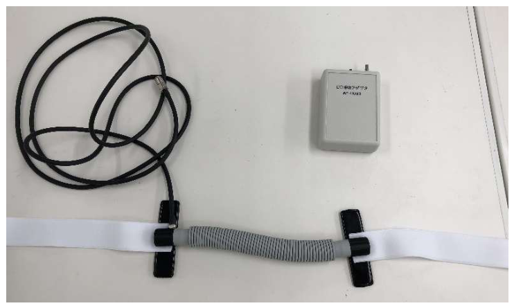
Figure 2.
Representative detection of P-, R-, and T-wave peaks using the PTC-based framework. ECG signals were band-pass filtered using a 0.4-Hz high-pass filter and a 40-Hz low-pass filter. The first 30 s of the analyzed segment are shown. The upper panel represents the supine condition and the lower panel the standing condition. Orange upward triangles, green circles, and red downward triangles indicate P-, R-, and T-wave peaks, respectively.
Figure 2.
Representative detection of P-, R-, and T-wave peaks using the PTC-based framework. ECG signals were band-pass filtered using a 0.4-Hz high-pass filter and a 40-Hz low-pass filter. The first 30 s of the analyzed segment are shown. The upper panel represents the supine condition and the lower panel the standing condition. Orange upward triangles, green circles, and red downward triangles indicate P-, R-, and T-wave peaks, respectively.
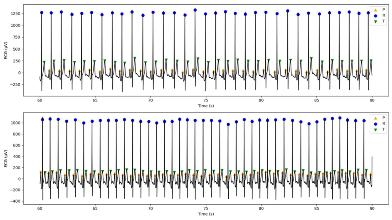
Figure 3.
PPI, RRI, TTI, and respiratory time series over the entire 360-s analysis segment in a representative participant. (a) Supine condition. (b) Standing condition. The signals correspond to 60–420 s after the start of each recording and are shown before application of the 0.03-Hz high-pass filter used for MVAR analysis.
Figure 3.
PPI, RRI, TTI, and respiratory time series over the entire 360-s analysis segment in a representative participant. (a) Supine condition. (b) Standing condition. The signals correspond to 60–420 s after the start of each recording and are shown before application of the 0.03-Hz high-pass filter used for MVAR analysis.
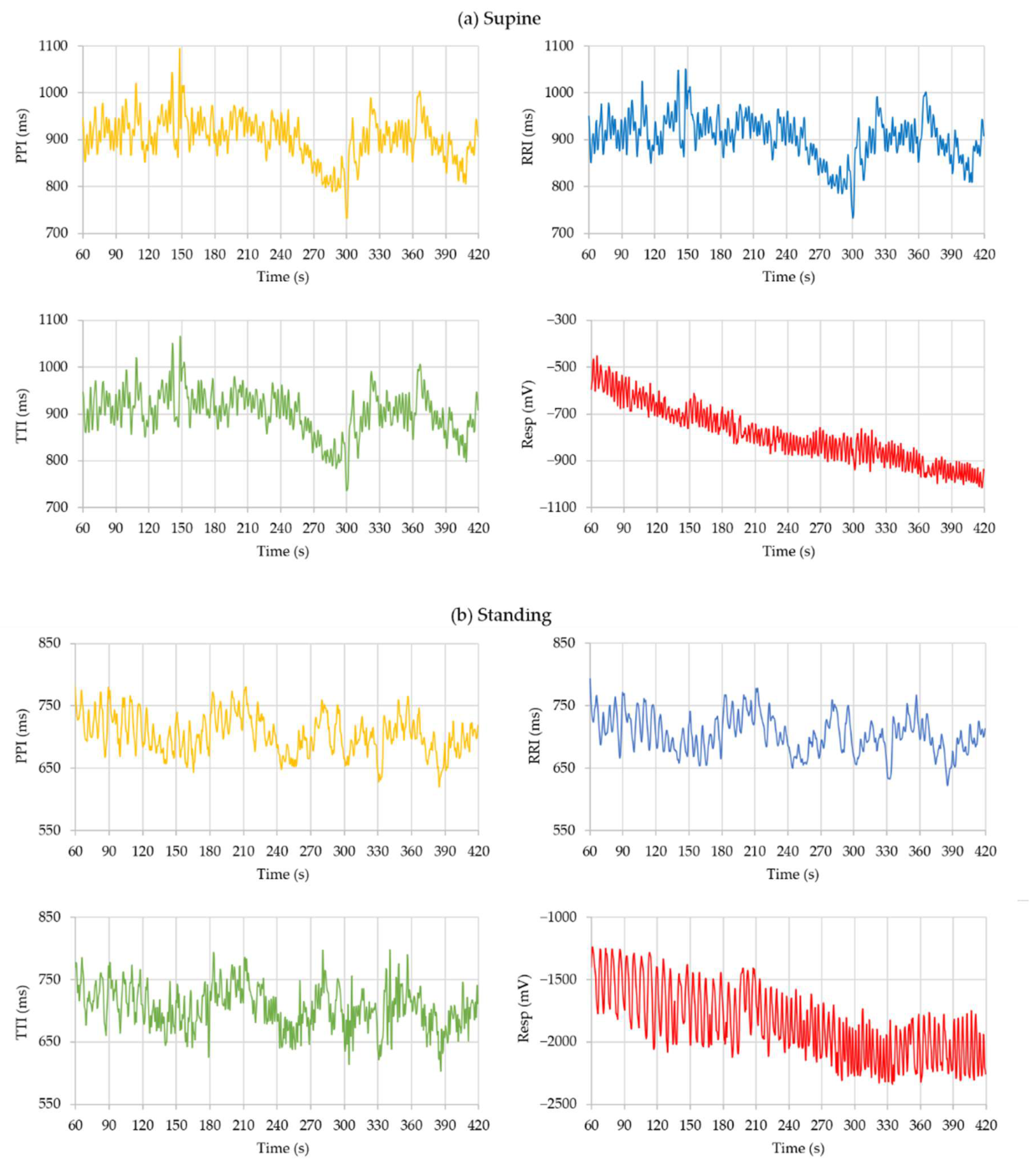
Figure 4.
Frequency-dependent component power and RPC ratios in Sub1 during the supine condition. Left: component-power spectra, Right: frequency-dependent RPC ratios. From top to bottom, the panels correspond to the PPI, RRI, TTI, and Resp targets, respectively.
Figure 4.
Frequency-dependent component power and RPC ratios in Sub1 during the supine condition. Left: component-power spectra, Right: frequency-dependent RPC ratios. From top to bottom, the panels correspond to the PPI, RRI, TTI, and Resp targets, respectively.
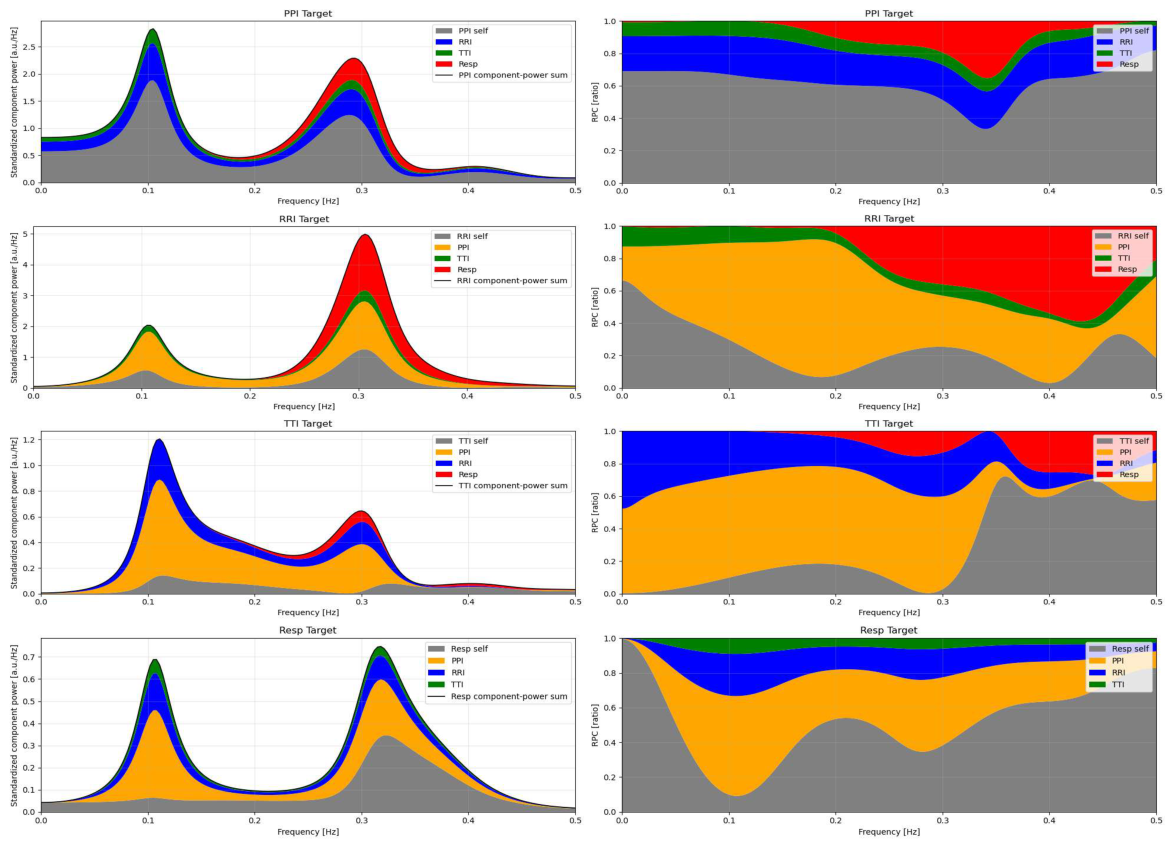
Figure 5.
Frequency-dependent component power and RPC ratios in Sub1 during the standing condition. Left: component-power spectra, Right: frequency-dependent RPC ratios. From top to bottom, the panels correspond to the PPI, RRI, TTI, and Resp targets, respectively.
Figure 5.
Frequency-dependent component power and RPC ratios in Sub1 during the standing condition. Left: component-power spectra, Right: frequency-dependent RPC ratios. From top to bottom, the panels correspond to the PPI, RRI, TTI, and Resp targets, respectively.
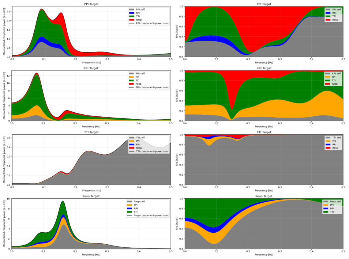
Figure 6.
Mean RPC topologies in the supine and standing conditions for the main analysis (n=13). Top left, supine LF; top right, supine HF; bottom left, standing LF; bottom right, standing HF. Nodes represent PPI, RRI, TTI, and respiration. Arrows indicate the direction of RPC, and self-loops indicate self-contributions. Numerical values denote mean band-integrated RPC values across the 13 participants. Asterisks indicate components showing significant differences between the supine and standing conditions after Benjamini–Hochberg FDR correction across all 32 LF- and HF-band comparisons (p*FDR < 0.05, p**FDR < 0.01).
Figure 6.
Mean RPC topologies in the supine and standing conditions for the main analysis (n=13). Top left, supine LF; top right, supine HF; bottom left, standing LF; bottom right, standing HF. Nodes represent PPI, RRI, TTI, and respiration. Arrows indicate the direction of RPC, and self-loops indicate self-contributions. Numerical values denote mean band-integrated RPC values across the 13 participants. Asterisks indicate components showing significant differences between the supine and standing conditions after Benjamini–Hochberg FDR correction across all 32 LF- and HF-band comparisons (p*FDR < 0.05, p**FDR < 0.01).
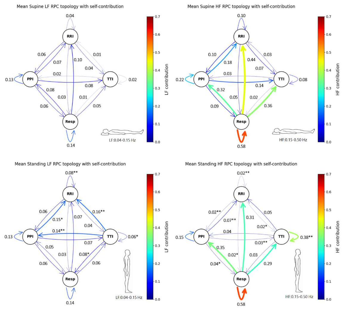

Table 1.
Example of temporal assignment of PPI, RRI, and TTI before interpolation.
| Beat | PPI time (s) | PPI (ms) | RRI time (s) | RRI (ms) | TTI time (s) | TTI (ms) |
| 1 | 59.05 | 916 | 59.246 | 916 | 59.488 | 914 |
| 2 | 59.956 | 906 | 60.152 | 906 | 60.394 | 906 |
| 3 | 60.832 | 876 | 61.028 | 876 | 61.27 | 876 |
| 4 | 61.744 | 912 | 61.94 | 912 | 62.178 | 908 |
Table 2.
Example of temporal alignment of PPI, RRI, TTI, and respiration on the common 2-Hz time grid.
Table 2.
Example of temporal alignment of PPI, RRI, TTI, and respiration on the common 2-Hz time grid.
| Common time (s) | PPI (ms) | RRI (ms) | TTI (ms) | Resp (μV) |
| 60 | 904 | 911 | 917 | −620.359 |
| 60.5 | 882 | 890 | 901 | −588.435 |
| 61 | 877 | 876 | 881 | −535.800 |
| 61.5 | 897 | 887 | 877 | −564.966 |
Table 3.
Descriptive characteristics of PPI, RRI, TTI, and respiratory peak frequency in the supine and standing conditions. Values for PPI, RRI, and TTI are presented as mean ± SD with 95% CIs, in ms. Respiratory peak frequency is presented in Hz.
Table 3.
Descriptive characteristics of PPI, RRI, TTI, and respiratory peak frequency in the supine and standing conditions. Values for PPI, RRI, and TTI are presented as mean ± SD with 95% CIs, in ms. Respiratory peak frequency is presented in Hz.
| Subject | PPI (ms) | RRI (ms) | TTI (ms) | Resp. peak freq. (Hz) | ||||
| Supine | Standing | Supine | Standing | Supine | Standing | Supine | Standing | |
| Sub1 | 904±47 (900–907) |
704±31 (702–707) |
904±47 (900–907) |
704±30 (702–707) |
904±48 (900–907) |
705±34 (702–707) |
0.337 | 0.156 |
| Sub2 | 1292±116 (1283–1300) |
963±66 (958–967) |
1292±116 (1283–1300) |
963±66 (958–967) |
1292±124 (1283–1301) |
963±69 (958–968) |
0.209 | 0.264 |
| Sub3 | 1077±48 (1073–1082) |
839±29 (837–842) |
1077±47 (1073–1082) |
839±28 (837–842) |
1078±47 (1073–1082) |
839±29 (837–842) |
0.272 | 0.305 |
| Sub4 | 821±24 (820–823) |
650±21 (648–651) |
821±24 (820–823) |
649±21 (648–651) |
822±25 (820–823) |
650±22 (648–651) |
0.184 | 0.128 |
| Sub5 | 1111±50 (1107–1114) |
799±29 (797–801) |
1111±51 (1107–1114) |
799±29 (797–801) |
1111±52 (1107–1115) |
799±29 (797–801) |
0.214 | 0.214 |
| Sub6 | 813±46 (809–816) |
730±42 (727–733) |
813±46 (809–816) |
730±43 (727–733) |
813±47 (809–816) |
730±44 (727–733) |
0.337 | 0.245 |
| Sub7 | 1027±109 (1019–1035) |
706±44 (703–709) |
1027±110 (1019–1035) |
706±44 (703–709) |
1027±111 (1019–1035) |
707±51 (703–710) |
0.134 | 0.153 |
| Sub8 | 700±28 (697–702) |
558±36 (554–562) |
700±28 (697–702) |
558±36 (554–562) |
700±29 (697–702) |
558±39 (554–562) |
0.194 | 0.233 |
| Sub9 | 683±27 (681–685) |
552±27 (550–554) |
683±27 (681–685) |
552±27 (550–554) |
683±27 (681–685) |
552±29 (550–554) |
0.339 | 0.234 |
| Sub10 | 970±60 (965–974) |
775±48 (771–778) |
970±60 (965–974) |
775±47 (771–778) |
970±60 (965–974) |
775±48 (771–778) |
0.223 | 0.303 |
| Sub11 | 983±97 (976–990) |
643±67 (638–648) |
983±97 (976–990) |
643±67 (638–648) |
983±98 (976–990) |
643±67 (638–648) |
0.184 | 0.125 |
| Sub12 | 1015±85 (1009–1022) |
765±49 (761–770) |
1015±84 (1009–1022) |
765±46 (761–769) |
1016±85 (1009–1022) |
765±49 (761–770) |
0.223 | 0.383 |
| Sub13 | 889±76 (884–895) |
674±34 (672–677) |
889±74 (884–895) |
674±32 (672–677) |
889±75 (884–895) |
674±34 (672–677) |
0.172 | 0.156 |
Table 4.
Selected MVAR model orders and residual diagnostic results for each participant and posture. FPE order indicates the model order selected by the FPE criterion. Final order indicates the order ultimately used for MVAR analysis after assessment of model stability. The minimum Ljung–Box p-value represents the minimum value obtained from the residual diagnostics. Multivariate whiteness was assessed using the adjusted multivariate Portmanteau test. ✓ indicates p > 0.05 for the multivariate whiteness test; ✕ indicates p ≤ 0.05. Residual diagnostic results were not used as exclusion criteria.
Table 4.
Selected MVAR model orders and residual diagnostic results for each participant and posture. FPE order indicates the model order selected by the FPE criterion. Final order indicates the order ultimately used for MVAR analysis after assessment of model stability. The minimum Ljung–Box p-value represents the minimum value obtained from the residual diagnostics. Multivariate whiteness was assessed using the adjusted multivariate Portmanteau test. ✓ indicates p > 0.05 for the multivariate whiteness test; ✕ indicates p ≤ 0.05. Residual diagnostic results were not used as exclusion criteria.
| Subject | Posture | FPE order |
Final order |
Min. Ljung–Box p |
Multivariate whiteness p |
Whiteness |
| Sub1 | Supine | 10 | 10 | 0.082 | <0.001 | ✕ |
| Standing | 8 | 8 | <0.001 | <0.001 | ✕ | |
| Sub2 | Supine | 11 | 11 | 0.566 | <0.001 | ✕ |
| Standing | 16 | 16 | 0.876 | 0.028 | ✕ | |
| Sub3 | Supine | 11 | 11 | 0.759 | 0.005 | ✕ |
| Standing | 8 | 8 | 0.771 | 0.007 | ✕ | |
| Sub4 | Supine | 11 | 11 | 0.333 | <0.001 | ✕ |
| Standing | 10 | 10 | 0.333 | <0.001 | ✕ | |
| Sub5 | Supine | 16 | 7 | <0.001 | <0.001 | ✕ |
| Standing | 9 | 9 | 0.002 | <0.001 | ✕ | |
| Sub6 | Supine | 13 | 13 | 0.942 | 0.009 | ✕ |
| Standing | 12 | 12 | 0.324 | 0.007 | ✕ | |
| Sub7 | Supine | 10 | 10 | 0.699 | 0.028 | ✕ |
| Standing | 13 | 13 | 0.638 | 0.004 | ✕ | |
| Sub8 | Supine | 9 | 9 | 0.511 | 0.169 | ✓ |
| Standing | 6 | 6 | 0.193 | 0.072 | ✓ | |
| Sub9 | Supine | 11 | 8 | 0.137 | <0.001 | ✕ |
| Standing | 11 | 11 | 0.709 | 0.008 | ✕ | |
| Sub10 | Supine | 9 | 9 | 0.117 | <0.001 | ✕ |
| Standing | 9 | 9 | 0.01 | 0.001 | ✕ | |
| Sub11 | Supine | 14 | 5 | <0.001 | <0.001 | ✕ |
| Standing | 8 | 8 | 0.075 | <0.001 | ✕ | |
| Sub12 | Supine | 7 | 7 | 0.013 | <0.001 | ✕ |
| Standing | 8 | 8 | 0.053 | <0.001 | ✕ | |
| Sub13 | Supine | 14 | 14 | 0.406 | 0.141 | ✓ |
| Standing | 11 | 11 | 0.444 | 0.02 | ✕ |
Table 5.
Conventional HRV indices and respiratory peak frequency in the supine and standing conditions. Values are presented as mean ± SD for paired t-tests and median [IQR] for Wilcoxon signed-rank tests.
Table 5.
Conventional HRV indices and respiratory peak frequency in the supine and standing conditions. Values are presented as mean ± SD for paired t-tests and median [IQR] for Wilcoxon signed-rank tests.
| Variable | Supine | Standing | Test | Statistic | p-value | Cohen’s dz |
| RRI (ms) | 945 ± 170 | 720 ± 113 | t | −9.83 | <0.001 | −2.73 |
| LF power (ms²) | 463 [1730] | 437 [477] | W | 17 | 0.048 | −0.59 |
| HF power (ms²) | 1061 [3545] | 147 [166] | W | 0 | <0.001 | −0.92 |
| LF/HF (ratio) | 0.783 [0.655] | 3.093 [4.162] | W | 0 | <0.001 | 1.21 |
| Respiratory peak freq. (Hz) | 0.232 ± 0.068 | 0.223 ± 0.078 | t | −0.38 | 0.71 | −0.11 |
Table 6.
RPC components showing significant differences between the supine and standing conditions. Values are mean ± SD for the main analysis (n=13). pFDR, Benjamini–Hochberg FDR-adjusted p-value. Cohen’s dz was calculated for Standing − Supine. The sensitivity analysis (n=10) excluded participants (sub4, sub7, and sub11) with respiratory peak frequencies within the LF band. ✓ indicates pFDR<0.05; ✕ indicates pFDR≥0.05.
Table 6.
RPC components showing significant differences between the supine and standing conditions. Values are mean ± SD for the main analysis (n=13). pFDR, Benjamini–Hochberg FDR-adjusted p-value. Cohen’s dz was calculated for Standing − Supine. The sensitivity analysis (n=10) excluded participants (sub4, sub7, and sub11) with respiratory peak frequencies within the LF band. ✓ indicates pFDR<0.05; ✕ indicates pFDR≥0.05.
| Band | Target | Edge | Supine (n=13) |
Standing (n=13) |
pFDR (n=13) |
Cohen’s dz (n=13) |
pFDR (n=10) |
Cohen’s dz (n=10) |
| LF | PPI | TTI→PPI | 0.02±0.01 | 0.14±0.14 | 0.002 | 0.94 | 0.014 ✓ | 0.91 |
| RRI | PPI→RRI | 0.07±0.05 | 0.15±0.12 | 0.024 | 0.84 | 0.106 ✕ | 0.73 | |
| RRI | RRI self | 0.04±0.03 | 0.08±0.05 | 0.002 | 0.83 | 0.014 ✓ | 0.82 | |
| RRI | TTI→RRI | 0.01±0.01 | 0.16±0.13 | 0.007 | 1.14 | 0.025 ✓ | 1.10 | |
| TTI | TTI self | 0.02±0.02 | 0.06±0.07 | 0.012 | 0.70 | 0.067 ✕ | 0.53 | |
| Resp | TTI→Resp | 0.01±0.01 | 0.08±0.10 | 0.012 | 0.67 | 0.067 ✕ | 0.59 | |
| HF | PPI | RRI→PPI | 0.10±0.04 | 0.02±0.03 | 0.002 | −1.56 | 0.007 ✓ | -1.87 |
| RRI | PPI→RRI | 0.18±0.10 | 0.07±0.06 | 0.008 | −1.09 | 0.057 ✕ | -0.99 | |
| RRI | RRI self | 0.10±0.06 | 0.02±0.01 | 0.002 | −1.37 | 0.018 ✓ | -1.25 | |
| TTI | PPI→TTI | 0.14±0.10 | 0.03±0.04 | 0.007 | −1.12 | 0.024 ✓ | -1.13 | |
| TTI | RRI→TTI | 0.07±0.06 | 0.02±0.02 | 0.012 | −0.97 | 0.040 ✓ | -0.99 | |
| TTI | TTI self | 0.08±0.10 | 0.38±0.29 | 0.002 | 1.07 | 0.024 ✓ | 1.15 | |
| Resp | PPI→Resp | 0.09±0.06 | 0.04±0.04 | 0.018 | −0.89 | 0.014 ✓ | -1.33 | |
| Resp | RRI→Resp | 0.05±0.05 | 0.02±0.01 | 0.012 | −0.79 | 0.014 ✓ | -1.01 |
Table 7.
Robustness of significant posture-related RPC components to P- and T-wave timing jitter in the main analysis (n=13). Off indicates the jitter-off condition. P and T indicate P-wave and T-wave timing jitter, respectively. Jitter amplitudes are expressed in milliseconds (ms). ✓ indicates that the posture-related difference remained significant after Benjamini–Hochberg FDR correction (pFDR<0.05); ✕ indicates pFDR≥0.05.
Table 7.
Robustness of significant posture-related RPC components to P- and T-wave timing jitter in the main analysis (n=13). Off indicates the jitter-off condition. P and T indicate P-wave and T-wave timing jitter, respectively. Jitter amplitudes are expressed in milliseconds (ms). ✓ indicates that the posture-related difference remained significant after Benjamini–Hochberg FDR correction (pFDR<0.05); ✕ indicates pFDR≥0.05.
| Band | Target | Edge | Off | P ±2 | P ±4 | P ±6 | P ±8 | P ±10 | T ±2 | T ±4 | T ±6 | T ±8 | T ±10 |
| LF | PPI | TTI→PPI | ✓ | ✓ | ✓ | ✓ | ✓ | ✓ | ✓ | ✓ | ✓ | ✓ | ✓ |
| RRI | PPI→RRI | ✓ | ✕ | ✕ | ✕ | ✕ | ✕ | ✕ | ✕ | ✕ | ✕ | ✕ | |
| RRI | RRI self | ✓ | ✕ | ✕ | ✕ | ✕ | ✕ | ✕ | ✕ | ✕ | ✕ | ✕ | |
| RRI | TTI→RRI | ✓ | ✓ | ✓ | ✓ | ✓ | ✓ | ✓ | ✓ | ✓ | ✓ | ✓ | |
| TTI | TTI self | ✓ | ✓ | ✓ | ✓ | ✕ | ✕ | ✕ | ✕ | ✕ | ✕ | ✕ | |
| Resp | TTI→Resp | ✓ | ✓ | ✓ | ✓ | ✓ | ✓ | ✓ | ✓ | ✓ | ✕ | ✕ | |
| HF | PPI | RRI→PPI | ✓ | ✓ | ✓ | ✓ | ✓ | ✓ | ✓ | ✓ | ✓ | ✓ | ✓ |
| RRI | PPI→RRI | ✓ | ✓ | ✓ | ✓ | ✓ | ✓ | ✓ | ✓ | ✓ | ✕ | ✕ | |
| RRI | RRI self | ✓ | ✓ | ✓ | ✓ | ✓ | ✓ | ✓ | ✓ | ✓ | ✓ | ✓ | |
| TTI | PPI→TTI | ✓ | ✓ | ✓ | ✓ | ✓ | ✓ | ✓ | ✓ | ✓ | ✓ | ✓ | |
| TTI | RRI→TTI | ✓ | ✓ | ✓ | ✓ | ✓ | ✓ | ✓ | ✓ | ✓ | ✓ | ✓ | |
| TTI | TTI self | ✓ | ✓ | ✓ | ✓ | ✓ | ✓ | ✓ | ✓ | ✓ | ✓ | ✓ | |
| Resp | PPI→Resp | ✓ | ✓ | ✓ | ✓ | ✓ | ✓ | ✓ | ✓ | ✓ | ✓ | ✓ | |
| Resp | RRI→Resp | ✓ | ✓ | ✓ | ✓ | ✓ | ✓ | ✓ | ✓ | ✓ | ✓ | ✓ |
Disclaimer/Publisher’s Note: The statements, opinions and data contained in all publications are solely those of the individual author(s) and contributor(s) and not of MDPI and/or the editor(s). MDPI and/or the editor(s) disclaim responsibility for any injury to people or property resulting from any ideas, methods, instructions or products referred to in the content. |
© 2026 by the authors. Licensee MDPI, Basel, Switzerland. This article is an open access article distributed under the terms and conditions of the Creative Commons Attribution (CC BY) license.
Copyright: This open access article is published under a Creative Commons CC BY 4.0 license, which permit the free download, distribution, and reuse, provided that the author and preprint are cited in any reuse.