
Submitted:
10 September 2026
Posted:
11 September 2026
You are already at the latest version
Abstract
The Curie isothermal surface (CIS) provides important information on crustal magnetic structures and thermal states. Conventional magnetic anomaly spectral methods for CIS inversion commonly rely on manually selected spectral parameters, leading to considerable subjectivity and uncertainty. This study proposes an adaptive CIS inversion method based on multiple geophysical constraints and Bayesian optimization. The method integrates de-fractal spectral analysis with a Tree-structured Parzen Estimator (TPE) to jointly optimize the fractal index, moving-window size, and spectral fitting ranges for estimating the top and centroid depths of the magnetic layer. Multiple constraints, including heat flow, magnetic anomaly characteristics, spatial distribution consistency, inversion uncertainty, and effective data coverage, are incorporated into the objective function. Synthetic experiments show that the proposed method improves inversion accuracy, reducing RMSE and MAE by 25.8% and 28.2%, respectively, compared with the conventional fixed-parameter method. Application to the Ordos Basin and surrounding regions reveals CIS depths of 22–40 km, with deeper values in the basin interior and Yangtze Craton and shallower values in surrounding tectonic zones. The CIS distribution shows consistency with crustal structures, heat flow, and seismicity, providing insights into regional thermal states and tectonic evolution.
Keywords:
curie isothermal surface
; heat flow
; Bayesian optimization
; de-fractal spectral
; ordos basin
1. Introduction
The thermal structure of the lithosphere provides a fundamental basis for understanding the composition, rheological properties, tectonic deformation, and deep geodynamic processes of the continental lithosphere, and is of considerable significance for geothermal resource assessment, tectonic stability evaluation, and studies of geodynamic evolution [1,2]. Surface heat-flow and geothermal-gradient observations directly reflect the thermal state of the shallow crust and therefore constitute important constraints on lithospheric thermal structure [3]. However, in tectonically complex regions, heat-flow observations are spatially uneven, and their ability to characterize large-scale deep thermal structure continuously is limited by both sparse sampling and local disturbances [4,5]. Crustal temperature generally increases with depth. When magnetic minerals reach their Curie temperature, ferromagnetism gradually transitions to paramagnetism, resulting in a marked decrease in crustal magnetization. The lower boundary of the effective magnetic layer inferred from magnetic anomalies is commonly referred to as the Curie Isothermal Surface (CIS). The CIS is jointly influenced by crustal temperature, magnetic mineral composition, and the structure of the magnetic basement, and thus represents an important geophysical interface for investigating lithospheric thermal structure [5,6,7,8].
Magnetic-anomaly spectral analysis is a commonly used method for estimating the CIS. Its basic principle is to use the relationship between the slopes of the power spectrum over different wavenumber ranges and the burial depths of magnetic sources to estimate the top and centroid depths of the magnetic layer, from which the depth to the bottom of the magnetic layer is further derived [9,10,11]. However, magnetic anomalies result from the superposition of magnetic bodies with different spatial scales, burial depths, and magnetization intensities, leading to non-uniqueness in their spectral characteristics [12,13]. In practical applications, the conventional centroid method and its modified variants generally require manual parameter selection, causing the inversion results to be influenced by empirical judgment and thereby reducing their objectivity [14].
In recent years, automated optimization methods have demonstrated strong global search capabilities in geophysical inversion and spatial prediction, particularly for optimization problems involving computationally expensive objective functions, nonlinear and multimodal parameter spaces, and discrete variables [15,16,17]. To reduce the influence of subjective parameter selection in conventional spectral inversion, this study proposes an adaptive CIS inversion method based on multiple constraints and Bayesian optimization. Within the de-fractal spectral framework, a Tree-structured Parzen Estimator (TPE) is introduced to jointly optimize the fractal index, window size, and wavenumber fitting intervals for the top and centroid depths of the magnetic layer, thereby enabling adaptive searching of the spectral parameters.
2. Data
2.1. Magnetic Anomaly Data
This study uses the global gridded magnetic anomaly dataset EMAG2v3 released by the National Centers for Environmental Information (NCEI). The dataset integrates shipborne, airborne, satellite, and geomagnetic observatory measurements. For the shipborne and airborne magnetic survey data, the effects of the main geomagnetic field and external magnetic fields were removed using Comprehensive Model 4, while the long-wavelength magnetic anomaly components were supplemented using the satellite lithospheric magnetic field model MF7. EMAG2v3 has a spatial resolution of 2′. In this study, the product referenced to a uniform altitude of 4 km was used and resampled to a spatial resolution of 0.1°. The spatial distribution of magnetic anomalies in the study area is shown in Figure 1.
The magnetic anomalies in the study area exhibit distinct spatial zonation. The main part of the Ordos Basin is characterized predominantly by broad positive and negative anomaly belts, whereas the amplitudes and spatial patterns of magnetic anomalies are more complex in the surrounding tectonic regions. Previous studies have shown that the sedimentary cover of the Ordos Basin is weakly magnetic and that regional magnetic anomalies are mainly controlled by the magnetic structure of the crystalline basement, with different magnetic anomaly belts showing good spatial correspondence with the regional basement structure [18,19]. Therefore, magnetic anomalies provide prior information on spatial variations in the magnetic structure of the study area and are used in this study as one of the constraints for CIS inversion parameter optimization.
2.2. Measured Heat-Flow Data
The measured heat-flow data were obtained from the China Terrestrial Heat Flow Database [20,21,22,23,24], as shown in Figure 2. In this study, the heat-flow observations were not interpolated to generate a continuous heat-flow field; instead, they were used only as constraint points at their corresponding spatial locations for objective-function calculation and result evaluation. To make full use of the limited measured heat-flow data, a five-fold cross-validation scheme was adopted. In each fold, 80% of the heat-flow observations were used as the optimization set for objective-function calculation and Bayesian parameter search, while the remaining 20% were used as the validation set to evaluate the inversion results. After completion of the five-fold cross-validation, Bayesian optimization was rerun using all measured heat-flow observations, and the optimal parameters obtained from the full dataset were adopted.
2.3. Other Geophysical Data
To investigate the relationships between the CIS, regional crustal structure, and present-day tectonic activity, Bouguer gravity anomaly, Moho depth, topography, and earthquake data were incorporated as auxiliary datasets. The Bouguer gravity anomaly data were obtained from the global gravity field model WGM2012 [25,26]. Moho depth, upper-crustal thickness, middle-crustal thickness, and topographic data were derived from the CRUST1.0 global crustal model [27]. The earthquake dataset mainly consists of magnitude records for events occurring within the study area since 1900 [28,29,30].
3. Methods
3.1. De-Fractal Spectral Method
Crustal magnetization exhibits fractal characteristics in the horizontal direction, and its power spectrum decays with wavenumber according to a power law [31,32]. The observed power spectrum EF(k) can be expressed as the product of the equivalent power spectrum ER(k) under a random magnetization model and the fractal term [33]:
Where k is the radial wavenumber and α is the fractal index. Let Zt denote the depth to the top of the magnetic layer, Z0 the centroid depth, and Zb the CIS depth. Zt and Z0 are estimated separately using the approximately linear relationships over different wavenumber ranges, for which the logarithmic spectra vary approximately linearly with k:
Least-squares linear fitting is performed for lnER(k) over the wavenumber interval [kt1,kt2] and for ln(ER(k)/k) over [k01,k02]:
Where st and s0 are the corresponding fitted slopes. The CIS depth Zb is then calculated as:
3.2. TPE Optimizer and Sampling Strategy
In CIS inversion, different combinations of the fractal index, window size, and wavenumber fitting intervals can all affect the inversion results. This optimization problem is characterized by high dimensionality, nonlinearity, and discrete variables, making Bayesian optimization well suited for parameter searching [30]. In this study, the Tree-structured Parzen Estimator (TPE) implemented in the Optuna framework was adopted as the sampler [31]. Let x denote the parameter combination to be optimized and y the corresponding objective-function value. TPE estimates p(x|y) and thereby constructs a probabilistic model of the objective function p(y|x). Based on the results of previous trials, the samples are divided into a better-performing set and a non-optimal set according to an objective-function threshold y*, and their probability density functions are modeled separately:
Where l(x) represents the parameter distribution corresponding to the better-performing samples, whereas g(x) represents the parameter distribution of the remaining samples. At each iteration, TPE selects the candidate parameter set that maximizes l(x)/g(x), i.e., the parameter combination that is more likely to produce a lower loss value:
3.3. Construction of the Objective Function
Bayesian optimization was used to search for the fractal parameter, moving-window size, and spectral fitting wavenumber ranges. The parameter vector to be optimized is defined as:
Where α is the fractal index, W is the window size, and [kt1,kt2] and [k01,k02] are the spectral fitting wavenumber ranges for the top and centroid depths of the magnetic layer, respectively. The composite objective function is defined as:
Where Lg is the magnetic-anomaly prior constraint term, Lp is the fitting term for the CIS converted from heat flow, Ls is the spatial-distribution constraint term, Lu is the uncertainty constraint term, and Lm is the valid-point coverage penalty term. λ denotes the weight assigned to the corresponding constraint term. During construction of the objective function, constraints are imposed only at locations with measured heat-flow data. After the parameters for all blocks have been determined, the CIS is calculated over the entire study area.
3.3.1. Magnetic-Anomaly Prior Constraint Term Lg
To preserve the information on deep magnetic structure reflected by the magnetic anomalies, a three-class prior representing deep, intermediate, and shallow CIS depths was established on the basis of the magnetic anomalies within each block. The 33rd and 66th percentiles of magnetic anomalies across all blocks were used as classification thresholds to distinguish the deep, intermediate, and shallow classes, yielding the prior CIS depth for each block:
The corresponding parameters were determined from the 33rd and 66th percentiles of the CIS values converted from measured surface heat flow. For the i th constraint point, the measured surface heat flow was converted into the corresponding reference CIS depth using a conductive radiogenic heat-production model [36]. The relationship between surface heat flow and CIS depth is given by [37]:
Where K is the volumetric vertical thermal conductivity of the magnetic layer and is set to 2.62 W/(m℃). Tc and Ts are the Curie temperature and surface temperature, respectively, and are set to 580℃ and 15℃. H0 is the surface heat-production rate, set to 2.85μW/m3, and hr is the characteristic depth of heat production, set to 13.8 km [7]. According to the difference between and the prior CIS depth of the corresponding block, the reliability weight of each observation point is defined as:
For a given block, let the median CIS depth of all valid inversion points be , The magnetic-anomaly prior constraint term is then defined as:
Where and are the lower and upper bounds of the prior CIS depth, respectively, defined as the 5th and 95th percentiles of the heat-flow-derived reference CIS values. and are soft-constraint coefficients. Because there is no strict one-to-one relationship between magnetic-anomaly amplitude and CIS depth, this term is implemented as a soft penalty to reduce the weight of parameter combinations that strongly deviate from the regional magnetic-anomaly background.
3.3.2. Heat-Flow-Derived Curie Isothermal Surface Fitting Term Lp
The CIS fitting term for the i th constraint point is represented by the weighted root mean square error:
Where Nv is the number of valid inversion points.
3.3.3. Spatial-Distribution Constraint Term Ls
Experimental tests showed that when only pointwise RMSE is used as the objective function, the overall error may remain small while local depth relationships and spatial variations become unreasonable. Therefore, the spatial-distribution constraint was constructed from three aspects: pairwise depth differences, spatial correlation, and relative depth ordering:
where Lpair is the pairwise depth-difference error term, Lcorr is the spatial-correlation constraint term, Lsign is the relative depth-ordering constraint term, and γ denotes the corresponding weighting coefficients. These terms are expressed as:
where P denotes the set of valid point pairs, ωij=1/(dij+0.05) is the weighting factor, and dij is the distance between two points. ρ is the Pearson correlation coefficient between the inverted and constrained values, and σref is the standard deviation of the CIS constraint values and inversion values. rmis represents the proportion of point pairs for which the relative shallow–deep or high–low relationship is reversed, and I is the indicator function.
3.3.4. Uncertainty Constraint Term Lu
The CIS uncertainty ΔZb at each valid point was obtained by propagating the standard errors of the spectral fitting slopes, and the uncertainty constraint term Lu was constructed as:
Where Zb is the mean uncertainty of all valid points and λu,i denotes the corresponding weighting coefficient. Equation (16) imposes an additional penalty on results with uncertainties exceeding 5 km and a stronger penalty on those exceeding 10 km.
3.3.5. Valid-Point Coverage Penalty Term Lm
Let N be the total number of constraint points. The valid-point coverage penalty term is expressed as:
When certain parameter combinations result in insufficient data within the moving window, spectral fitting failure, or inversion results outside the reasonable range, the number of valid points Nv decreases and Lm increases accordingly. This encourages TPE to preferentially select parameter combinations capable of covering a larger number of observation points.
4. Experimental Testing and Algorithm Validation
4.1. Determination of Objective-Function Weights and Sensitivity Analysis
A combination of nested spatial cross-validation and TPE was adopted to jointly optimize the weights of the individual constraint terms and their internal subterms in the objective function. In the outer TPE optimization, 24 candidate weight combinations were generated simultaneously within the predefined ranges and initially screened using two-fold spatial cross-validation. Based on the spatial coordinates of the reference points, the study area was divided into two spatial subregions. In each fold, one subregion was used as the training region, within which block-wise Bayesian inversion was rerun, while the reference points in the other subregion were used to evaluate predictive performance. The inner Bayesian optimization was used only to search for the fractal parameter, moving-window size, and spectral fitting wavenumber ranges, with their search ranges kept unchanged, thereby maintaining independence between weight selection and physical-parameter inversion.
After the initial screening, the five candidate weight combinations with the best overall evaluation performance were selected and, together with the initial weight combination, further evaluated using three-fold spatial cross-validation. The final objective-function weights were determined according to the combined performance of prediction error, mean uncertainty, and valid-point coverage in the test regions. Through the above joint optimization and spatial cross-validation procedure, the optimal weight combination applicable to the study area was obtained within the predefined parameter ranges, as listed in Table 1.
4.2. Objective-Function Ablation Experiment Design
A small-area synthetic spectral experiment was designed to evaluate the ability of the proposed method to recover the spatial morphology, local anomalies, and overall depth trends of the CIS. A 4°×4° synthetic region was constructed, within which a true Curie isotherm depth field containing both regional variation trends and local anomalous perturbations was generated. The corresponding magnetic anomalies were then produced from the prescribed true CIS field. In the experiment, the fractal index was set to α=1.2. Random noise perturbations were incorporated during spectral construction by adding Gaussian random noise with an amplitude equivalent to 14% of the signal standard deviation, in order to simulate disturbances caused by observational errors, local anomalies, and instability in spectral estimation during practical spectral analysis. Twenty percent of the reference points were randomly sampled from the synthetic true CIS field and used as reference depths corresponding to simulated heat-flow constraints for calculation of the Bayesian-optimization objective function.
To evaluate the effects of different levels of parameter optimization and constraint information on the inversion results, a conventional fixed-parameter method and three progressively optimized schemes were designed. In the conventional method, the fractal index, window size, and fitting wavenumber intervals were fixed at α=1, windows_size=3°, kt1=0.03 km-1, kt2=0.08 km-1, k01=0.005 km-1, k02=0.055 km-1. This parameter combination represents commonly used empirical fitting-band ranges in the conventional centroid method or modified centroid method [38]. In M1, the fractal index and window size were fixed, and only the fitting wavenumber intervals for Zt and Z0 were treated as parameters to be optimized. In M2, the fractal index, window size, and the two fitting wavenumber intervals were jointly optimized, with the fitting error relative to the heat-flow-derived reference CIS used as the primary optimization criterion. In M3, magnetic-anomaly priors, spatial-distribution consistency, inversion uncertainty, and valid-point coverage constraints were further introduced on the basis of M2, constituting the complete adaptive inversion method proposed in this study. The number of Bayesian-optimization trials was set to 150 for each of the three optimization schemes.
4.3. Synthetic Experiment Results
The spatial distributions of the experimental results (Figure 3) show that the conventional fixed-parameter method can recover the regional variation trend of the Curie isotherm depth, but tends to underestimate amplitudes or produce spatial offsets in areas of local shallow and deep anomalies. In comparison, the proposed method, through joint optimization of the fractal index, window size, and fitting wavenumber ranges, more effectively recovers the regional depth variations and local anomalous features of the synthetic CIS. Areas with large errors are markedly reduced, indicating that the adaptive fitting-band selection strategy improves inversion stability at different spatial locations. The overall error of the proposed method is reduced, and errors near the boundaries of local anomalies are also decreased, indicating a better balance between spectral stability and preservation of local structural features.
Table 2 presents a quantitative comparison among the conventional fixed-parameter method, the method in which only the wavenumber intervals were optimized, the full-parameter Bayesian optimization method, and the final method proposed in this study. For the conventional fixed-parameter method, the RMSE and MAE are 1.24 km and 1.03 km, respectively, while the mean relative error and median relative error are 3.12% and 2.88%, respectively. The method that optimizes only the wavenumber intervals does not yield improved results, with the RMSE increasing to 1.37 km. This indicates that, when the fractal index and window size are fixed, optimizing only the fitting wavenumber ranges for Zt and Z0 cannot stably improve the inversion performance.
When the fractal index, window size, and wavenumber fitting ranges are jointly included in Bayesian optimization, the RMSE of M2 decreases to 0.98 km and the MAE decreases to 0.79 km, indicating that joint multi-parameter optimization can effectively reduce errors associated with empirical parameter selection. After further introducing magnetic-anomaly priors, spatial-distribution consistency, inversion uncertainty, and valid-point coverage constraints, the RMSE and MAE of the complete method decrease to 0.92 km and 0.74 km, respectively, representing reductions of approximately 25.8% and 28.2% relative to the conventional method. Meanwhile, the mean relative error decreases from 3.12% to 2.23%, and the median relative error decreases from 2.88% to 1.88%, indicating that the proposed method outperforms the conventional fixed-parameter method in terms of both overall accuracy and error level.
5. Curie Isothermal Surface in the Ordos Basin
5.1. Block Division of the Ordos Region
The study area spans the Ordos Basin and several surrounding tectonic units, which exhibit pronounced differences in magnetic basement structure, magnetic anomaly characteristics, and deep crustal structure. Applying a uniform set of spectral parameters to the entire study area would make it difficult to accommodate the distinct magnetic-anomaly spectral characteristics of different tectonic regions. Therefore, prior to parameter optimization, the study area was divided into multiple blocks, allowing spectral parameters to be searched independently within each block. This reduces the influence of regional structural differences on the selection of uniform parameters and provides a spatial basis for the subsequent adaptive inversion.
The block division follows different criteria for the basin interior and its surrounding regions, as shown in Figure 4. In tectonically active areas outside and around the Ordos Basin, block boundaries were primarily determined according to the regional tectonic framework, major tectonic units, and the spatial distribution of large-scale faults. The interior of the Ordos Basin is relatively tectonically stable, although differences in the crystalline basement remain among different regions. Because the sedimentary cover of the basin is weakly magnetic and the regional magnetic anomalies are mainly controlled by the magnetic structure of the crystalline basement, the basin interior was further subdivided with reference to previously reported basement structures and magnetic-anomaly zoning characteristics [19]. On this basis, subsequent TPE parameter optimization was conducted independently for each block to obtain parameter combinations adapted to the magnetic-anomaly spectral characteristics of different regions.
5.2. Inversion Results and Parameter Characteristics
To evaluate the five-fold cross-validation results, the inverted CIS at each validation point was substituted into Eq. (10), and heat flow was calculated using the same thermophysical parameters and then compared with the measured heat flow. The RMSE was 35.9462±1.2174 mW/m2, and the MAE was 32.4984±0.6750 mW/m2. After completion of the cross-validation, Bayesian optimization was rerun using all measured heat-flow points, and the parameters obtained from full-data optimization were used to perform the final regional inversion. The resulting CIS and associated parameter distributions are shown in Figure 5.
Figure 5 shows the distributions of the CIS, optimal window size, fractal index, and inversion uncertainty in the Ordos Basin and surrounding regions, together with representative spectral fitting results for the top and centroid depths of the magnetic layer. The CIS is generally deeper within the main body of the Ordos Basin, with a local deep zone developed near the Hetao region in the north. In parts of the central and northern basin, the CIS reaches 36–40 km. In contrast, the Qilian Fold System, northeastern Tibetan Plateau, Qinling Orogen, Weihe Graben, Taihang tectonic belt, and North China Plain are characterized by relatively shallow CIS values, locally ranging from approximately 22 to 30 km. This spatial pattern indicates pronounced differences in the CIS and deep thermal state between the stable interior of the Ordos Block and the surrounding tectonic belts.
Compared with inversion using uniform parameters throughout the entire study area, block-wise adaptive inversion better preserves depth variations among different tectonic units and reduces the smoothing effect of uniform parameters across tectonic boundaries and local anomalies. Figure 5(b) shows that the window size varies among tectonic units, indicating that a fixed window cannot simultaneously account for regional-scale deep information and local spatial resolution, whereas adaptive window selection allows the computational scale to be adjusted according to the magnetic-anomaly spectral characteristics of different blocks. Figure 5(c) shows that the fractal index varies among different basement units within the Ordos Basin, and pronounced differences are also observed between the basin interior and the surrounding orogenic belts, rift zones, and the eastern North China Craton. The fractal index reflects the decay characteristics of the magnetic-anomaly power spectrum, and its spatial variation indicates significant regional differences in the distribution of magnetization intensity, the complexity of magnetic sources, and spatial correlation.
Figure 5(d) shows that the CIS uncertainty is less than 5 km over most of the study area. Uncertainties are generally lower within the main part of the Ordos Basin, indicating relatively stable magnetic-anomaly spectra and good linear characteristics within the selected wavenumber intervals. Higher uncertainties are mainly concentrated near the southwestern and southeastern tectonic boundaries of the study area. The southwestern margin contains relatively few constraint points, whereas magnetic anomalies vary strongly in the southeastern tectonic boundary region. The superposition of spectral contributions from magnetic sources at different depths and spatial scales is therefore more complex, increasing the difficulty of identifying linear fitting segments. In the representative spectra shown in Figure 5(e) and 5(f), both the low-wavenumber and medium- to high-wavenumber ranges exhibit relatively clear near-linear relationships, indicating that Bayesian optimization can identify suitable fitting intervals for estimating Z0 and Zt from the candidate spectral ranges.
5.3. Comparison with Previous Results
Different inversion methods differ in their treatment of magnetic-anomaly data, assumptions regarding magnetic-layer models, and parameter-selection strategies. Consequently, the resulting CIS models are not completely consistent in terms of spatial resolution, degree of smoothing, and anomaly amplitude. Figure 6 presents the CIS results obtained using four methods, and Table 3 lists the corresponding evaluation metrics. To ensure comparability among the different CIS models, all four CIS models were sampled at the same heat-flow observation locations, and surface heat flow was calculated using the same thermophysical parameters and heat-conduction model.
The RMSE and MAE obtained using the method proposed in this study are close to those of the regional inversion by Gao et al. (2015) and lower than those of Li et al. (2017) and Zhou et al. (2024). The correlation coefficient is higher than those of Gao et al. (2015) and Zhou et al. (2024) and is generally comparable to that of Li et al. (2017). These results indicate that the proposed method improves the consistency between the inversion results and the spatial variation in heat flow while maintaining a regional-scale error level comparable to previous studies.
The global CIS reference model established by Li et al. (2017) using EMAG2 data was obtained by integrating and averaging results from multiple fixed windows. The resulting model exhibits good regional continuity and can stably characterize thermal-structure features at global and continental scales. In the Ordos region, this model shows the general pattern of a relatively deep CIS within the basin and a shallower CIS in the surrounding regions, which is broadly consistent with the results of this study. The present results exhibit more pronounced lateral variations along the southwestern, southern, and eastern margins of the Ordos Basin, particularly within several tectonic transition zones. This difference is related to the block-wise parameter optimization adopted for regional tectonic units and the incorporation of measured heat-flow constraints in this study. The similarity between the two results indicates that the present inversion preserves the stability of the regional background field, whereas the local differences reflect the different spatial-scale emphases of global-scale models and detailed regional inversions.
Gao et al. (2015) obtained the Curie point depth distribution in the Ordos region using a continual-model inversion method. Their results show that the interior of the Ordos Block is dominated by relatively deep values exceeding 32 km, in good agreement with the results of this study. Both studies indicate a deeper bottom boundary of the magnetic layer beneath the basin interior and a shallower boundary in the surrounding regions. The continual-model results exhibit a relatively complete high-value zone within the main body of the basin and further reveal local differences among different basement units within the basin. These differences reflect the distinct responses of continuous-interface recovery and block-wise spectral inversion to magnetic-anomaly information at different spatial scales.
The adaptive-window method proposed by Zhou et al. (2024) selects the optimal window according to the stability of the CIS with changing window size, effectively alleviating the difficulty of simultaneously capturing deep information and local spatial resolution with a fixed window. Their results exhibit relatively abundant local variations in some tectonic boundary zones and block-junction areas, reflecting the ability of adaptive windows to respond to magnetic structures at different scales. The overall variation trends along the western and southern margins of the basin and in the eastern transition zone are generally consistent with those obtained in this study, although the local gradients of variation are larger. This difference arises because, in addition to the window size, the present method simultaneously adjusts the fractal index and the fitting wavenumber intervals for the top and centroid depths of the magnetic layer, while heat-flow and spatial-structure constraints are used to comprehensively screen different parameter combinations. The resulting CIS therefore preserves variations in tectonic transition zones while maintaining relatively good continuity between adjacent regions. Profiles of the four results along A–A′ are shown in Figure 7.
5.4. Regional Differences Between the Curie Isothermal Surface and Crustal Structure
Comparison along the A–A′ profile (Figure 7.) shows that the CIS derived in this study exhibits pronounced spatial differences relative to Moho depth and Bouguer gravity anomalies. To further examine the regional distribution of these differences across the entire study area, the relationships between the CIS and regional crustal structure were analyzed in combination with Bouguer gravity anomalies, Moho depth, and upper- and middle-crustal thicknesses, as shown in Figure 8. The Bouguer gravity anomaly generally increases from west to east. The northeastern Tibetan Plateau and the Qilian Fold System are dominated by strong negative anomalies, whereas the main part of the Ordos Basin is characterized mainly by moderate negative anomalies, which gradually transition eastward to weak negative and positive anomalies toward the Taihang Mountains and North China Plain. Correspondingly, crustal thickness also exhibits a pronounced east–west variation. Moho depth is greatest beneath the northeastern Tibetan Plateau and the Qilian Fold System, where the total crustal thickness reaches approximately 48–54 km. The crust beneath the main part of the Ordos Basin is approximately 40–45 km thick, whereas farther east beneath the Taihang Mountains and North China Plain, crustal thickness gradually decreases to approximately 30–39 km. The thicknesses of the upper and middle crust also generally decrease from west to east, locally exceeding 20 km in the western tectonic region but becoming distinctly thinner in the eastern region. These characteristics indicate that Bouguer gravity anomalies and crustal thickness show good regional-scale correspondence across the study area, jointly reflecting the structural transition from the thickened crust of the northeastern Tibetan Plateau to the thinner crust beneath the North China Plain.
Within the main part of the Ordos Basin, the CIS generally shows good spatial correspondence with crustal structure. The central and northern parts of the basin are characterized by relatively thick crust and a generally deep CIS with good spatial continuity. Toward the eastern basin and the Taihang Mountains–Shanxi Rift, crustal thickness gradually decreases and the CIS also becomes shallower overall. In contrast, a more pronounced vertical structural difference occurs near the boundary between the northeastern Tibetan Plateau and the western Ordos Basin. In this region, Moho depth generally exceeds 48 km, and the upper and middle crust are also significantly thickened, whereas the CIS is mainly located at approximately 25–32 km, markedly shallower than the Moho and close to the base of the upper-crustal depth range. This feature indicates that, although the western tectonic region has undergone substantial crustal thickening, the effective magnetic layer has not increased synchronously with total crustal thickness and remains mainly confined to the upper crust and the upper part of the middle crust. This pronounced separation between the CIS and crustal thickness provides an important basis for further analysis of the thermal state and tectonic processes within the thickened crust of this region.
6. Discussion
The results of this study show pronounced differences in CIS distribution between the main part of the Ordos Basin and its eastern and western margins, reflecting the influences of different tectonic processes, including stable cratonic evolution, plateau–craton interaction, and reworking of the eastern North China Craton, on the regional crustal thermal state and magnetic structure, as illustrated in Figure 9.
The CIS in the central part of the Ordos Basin is generally deep, locally reaching 36–40 km, and corresponds spatially to a relatively deep Moho and smooth Bouguer gravity anomalies. This region developed on Archean–Paleoproterozoic crystalline basement, and large active faults and Phanerozoic magmatic activity are relatively weak within the basin, with present-day tectonic deformation concentrated mainly along its margins. Magnetotelluric and seismic imaging results indicate that the interior of the Ordos Block is generally characterized by high resistivity and high seismic velocities, suggesting relatively stable crustal and lithospheric structures and the preservation of overall stable crustal and lithospheric characteristics [39,40]. Such conditions are favorable for maintaining a relatively low regional geothermal gradient and therefore a deep CIS. In addition, the relatively intact crystalline basement and lower-crustal structure preserved within the basin provide a material basis for a thick effective magnetic layer. Therefore, the deep CIS in the central basin mainly reflects the relatively low thermal state and thick effective magnetic layer formed during the long-term evolution of a stable craton.
The CIS beneath the eastern Ordos region and the Taihang Mountains–Shanxi Rift is distinctly shallower than that beneath the central basin. Since the Late Mesozoic, westward subduction of the Paleo-Pacific Plate and related geodynamic processes have been widely regarded as an important geodynamic background for lithospheric reworking and destruction of the eastern North China Craton [41]. Slab rollback and associated asthenospheric upwelling promoted thermochemical modification of the lithospheric mantle, resulting in thinning and replacement of the ancient lithosphere [42]. Cenozoic extension of the Shanxi Rift further facilitated regional lithospheric adjustment and changes in the deep thermal state [43], increasing the regional geothermal gradient and causing relative shallowing of the bottom boundary of the effective magnetic layer. Meanwhile, lithospheric thinning reduced crustal thickness, resulting in overall Moho uplift and a corresponding increase in Bouguer gravity anomalies. Therefore, the shallow CIS in the eastern study area reflects the combined effects of lithospheric thinning of the eastern North China Craton, enhanced deep thermal conditions, and Cenozoic extension under the geodynamic background of Paleo-Pacific subduction.
The Qinling Orogen records multiple stages of convergence and collision between the North China Craton and the Yangtze Craton. Lithospheric roots, crustal detachment structures, and pronounced lateral velocity variations revealed by deep seismic reflection and seismic tomography indicate that the ancient collision-related suture zone continues to control crustal deformation and deep structure along the southern margin [44,45]. Seismic imaging has identified an upper-mantle low-velocity anomaly extending eastward from the northeastern Tibetan Plateau between the Ordos Block and the Yangtze Craton. It has been suggested that the rigid lithospheric roots beneath the Ordos Block and Yangtze Craton jointly restrict the eastward migration of asthenospheric material, forcing it to undergo channelized flow along the Qinling tectonic belt [46,47]. The relatively high-velocity structure in the middle and lower crust of the western Qinling may impede further eastward migration of low-velocity crustal material, whereas low-velocity anomalies in the lithospheric mantle beneath the Weihe Graben and eastern Qinling reflect thermochemical modification of the upper mantle associated with asthenospheric activity [48]. Three-dimensional gravity and magnetic inversion of the Weihe Basin indicates that regional heat flow does not show an obvious correspondence with Moho uplift, and that Yanshan granitic bodies buried beneath the basin sediments and their radiogenic heat production may constitute an important crustal heat source [49]. Differences in basement composition and magnetic mineral content on the two sides of the Weihe Fault also influence the position of the bottom boundary of the effective magnetic layer. Therefore, the relatively shallow CIS along the southern margin of the Ordos Basin may be jointly influenced by inherited paleocollisional structures, channelized asthenospheric flow and upper-mantle modification, tectonic activity of the Weihe Graben, and radiogenic heat production from granitic crust.
The northern Ordos Basin and the southern margin of the Hetao region form a local deep-CIS zone, with values reaching 36–40 km in some areas. High-resolution seismic imaging indicates that the northern Ordos region is generally characterized by relatively high seismic velocities and weak lateral variations, suggesting that relatively stable cratonic crustal and lithospheric structures are still preserved in this area [50,51]. Recent ambient-noise imaging further reveals a NE-trending high-velocity zone in the middle crust of the central–northern Ordos region that corresponds spatially to the magnetic anomalies and represents mafic–ultramafic basement structures formed during the amalgamation of ancient microcontinental blocks [52]. The relatively low thermal state, together with the well-preserved and strongly magnetic crystalline basement, may favor the development of a thick effective magnetic layer, consistent with the deep CIS obtained in the northern part of the study area. Receiver-function and seismic imaging results show that the upper crust beneath the Hetao–Yinchuan rift system has undergone extension, whereas the middle and lower crust exhibit local thickening, and residual crustal roots formed during Late Mesozoic intracontinental orogenesis are still preserved beneath parts of the rift [53,54]. Evidence for localized lithospheric thinning and mantle thermal modification beneath the Hetao Rift–Yinshan tectonic belt indicates that the northern margin has undergone varying degrees of reactivation [55]. Therefore, the deep CIS beneath the northern basin and southern Hetao margin may be related to the stable magnetic basement and residual thickened crust, whereas local variations near the rift axis and tectonic boundaries may be associated with mantle thermal perturbations and lithospheric modification.
The CIS beneath the western Ordos region, northeastern Tibetan Plateau, and Qilian Fold System is markedly shallower than the Moho. In this region, the Moho locally reaches depths greater than 48–50 km and corresponds to pronounced negative Bouguer gravity anomalies, whereas the CIS is mainly 25–32 km deep, indicating a substantial difference between total crustal thickness and effective magnetic-layer thickness. The northeastern Tibetan Plateau continues to expand toward the east and northeast. Under the obstruction of the rigid Ordos Block, the left-lateral strike-slip motion along the Haiyuan Fault gradually weakens eastward and is transformed into thrust shortening and tectonic uplift in the Liupanshan region. Crustal shortening, thrust stacking, and middle- to lower-crustal thickening jointly contribute to Moho deepening and lower Bouguer gravity anomalies in the western region [51,56]. Seismic imaging has identified low shear-wave velocities and anisotropic structures beneath the northeastern Tibetan Plateau and adjacent Liupanshan region, suggesting that ductile flow in the middle and lower crust contributes to outward plateau expansion and crustal thickening [40,57]. Other studies, however, indicate pronounced lateral heterogeneity in crustal deformation in this region. Thickened high-velocity lower-crustal structures are present beneath both Liupanshan and the southwestern margin of the Ordos Block, suggesting that crustal thickening along the western margin may be accommodated jointly by upper-crustal thrust shortening, middle- to lower-crustal stacking, and localized ductile deformation rather than by a single continuous crustal-flow mechanism [51,58]. Deformation of the middle and lower crust, ductile shearing, crust–mantle interaction, and localized thermal perturbations within the boundary zone may jointly enhance the thermal state of the middle and lower crust, preventing the bottom of the effective magnetic layer from deepening synchronously with Moho deepening caused by tectonic crustal thickening.
Figure 10 shows the spatial distributions of surface heat flow converted from the inverted CIS using the heat-conduction model and earthquakes with M≥3 in the study area since 1900. Seismicity is generally concentrated around the margins of the Ordos Block and along major active tectonic belts, whereas relatively few earthquakes occur within the main body of the basin. This corresponds to the deeper CIS, lower converted heat flow, and weaker seismic activity in the central and northern parts of the basin. In contrast, numerous earthquakes are distributed along the western and southwestern margins of the basin, particularly along the northeastern Tibetan Plateau and the Qilian tectonic belt, showing good spatial correspondence with the shallow CIS and relatively high converted heat flow. In particular, along the western margin of the Ordos Basin, Moho depth can exceed 48–50 km, whereas the CIS is mainly 25–32 km, showing a pronounced separation between crustal thickness and the bottom boundary of the effective magnetic layer. These characteristics indicate that, during the interaction between the continued expansion of the northeastern Tibetan Plateau and the rigid Ordos Block, crustal thickening did not result in synchronous deepening of the effective magnetic layer. The northeastern Tibetan Plateau and the Qilian Fold System are simultaneously characterized by relatively high CIS-derived heat flow and concentrated seismic activity on the centennial timescale, in marked contrast to the lower heat flow and weaker seismicity within the main body of the Ordos Basin.
7. Conclusions
This study addresses the dependence of the fractal index, window size, and spectral fitting intervals on manual selection in conventional magnetic-anomaly spectral methods by developing a Bayesian adaptive inversion method under multiple constraints and applying it to CIS inversion in the Ordos Basin and surrounding regions. The main conclusions are as follows:
(1) Based on de-fractal spectral analysis, the fractal index, moving-window size, and fitting wavenumber intervals for the top and centroid depths of the magnetic layer were incorporated into a unified optimization parameter space and jointly searched using TPE, thereby replacing empirical manual parameter selection with adaptive joint determination. Surface heat flow, magnetic-anomaly priors, spatial distribution, uncertainty, and valid-point coverage were further introduced as constraints during parameter optimization, transforming parameter selection from single spectral fitting into comprehensive optimization constrained by multiple sources of information and allowing adaptation to the differences in magnetic-anomaly spectra among different tectonic units. The weight-sensitivity analysis and spatial cross-validation results show that the different constraint terms provide a reasonable balance among inversion accuracy, spatial stability, and valid-data coverage.
(2) Synthetic experiments show that optimizing only a subset of the spectral parameters does not consistently improve the inversion results, whereas joint optimization of the fractal index, window size, and fitting wavenumber intervals can significantly reduce errors associated with parameter selection. With the further inclusion of multiple constraints, the recovery of regional CIS variations and local anomalies is further improved. The RMSE and MAE of the proposed method are 0.92 km and 0.74 km, respectively, representing reductions of 25.8% and 28.2% relative to the conventional fixed-parameter method. The mean and median relative errors also decrease simultaneously, indicating that joint multi-parameter optimization and multi-constraint screening improve both the accuracy and stability of spectral inversion.
(3) The CIS in the Ordos Basin and surrounding regions is generally approximately 22–40 km deep. Relatively deep values occur in the central and northern parts of the basin, reaching 36–40 km in some areas, whereas the northeastern Tibetan Plateau, Qilian Fold System, Qinling–Weihe tectonic belt, and Taihang Mountains–Shanxi Rift are generally characterized by shallower values of 22–30 km. The relatively deep CIS beneath the main body of the basin corresponds to the well-preserved crystalline basement, relatively stable crustal structure, and lower thermal state. The shallow CIS in the eastern study area shows good spatial correspondence with lithospheric thinning of the eastern North China Craton and the extensional setting of the rift system. In the western study area, the northeastern Tibetan Plateau and Qilian Fold System exhibit a more pronounced vertical structural contrast: the Moho reaches depths of 48–50 km, whereas the CIS is mainly 25–32 km, indicating that tectonically thickened crust has not developed an effective magnetic layer that increases synchronously with total crustal thickness. This region is also characterized by relatively high heat flow and concentrated seismic activity, indicating a pronounced enhancement of the thermal state of the middle and lower crust during crustal thickening along the western margin of the Ordos Basin.
Author Contributions
Conceptualization, Q.F. and G.G.; methodology, Q.F. and G.G.; software, Q.F.; validation, Q.F., G.G., C.B. and L.W.; formal analysis, Q.F.; investigation, Q.F.; resources, G.G., C.B., L.W. and Z.W.; data curation, Q.F., G.G. and Z.W.; writing—original draft preparation, Q.F.; writing—review and editing, G.G., C.B., L.W. and Z.W.; visualization, Q.F.; supervision, G.G.; project administration, G.G.; funding acquisition, G.G. and C.B. All authors have read and agreed to the published version of the manuscript.
Funding
This research was funded by the National Natural Science Foundation of China under grants 41964004 and 42264005.
Institutional Review Board Statement
Not applicable.
Informed Consent Statement
Not applicable.
Data Availability Statement
Data available on request.
Acknowledgments
We are deeply grateful to the Associate Editor, and the two anonymous reviewers for their insightful comments and constructive suggestions.
Conflicts of Interest
The authors declare no conflicts of interest.
References
- Moisio, K.; Kaikkonen, P.; Beekman, F. Rheological structure and dynamical response of the DSS profile BALTIC in the SE Fennoscandian Shield. Tectonophysics 2000, 320, 175–194. [CrossRef]
- Wang, X.F.; Wang, K.Q.; Zhao, Z.X.; Xu, H.H.; Zhao, J.F.; Ren, Z.Q.; Zhang, J.Z. Three-dimensional thermal structure of the lithosphere and its relationship to surface structure in the South China Sea. Chin. J. Geophys. 2021, 64, 4105–4116. [CrossRef]
- Tanaka, A.; Okubo, Y.; Matsubayashi, O. Curie point depth based on spectrum analysis of the magnetic anomaly data in East and Southeast Asia. Tectonophysics 1999, 306, 461–470. [CrossRef]
- Jaupart, C.; Mareschal, J. Heat Generation and Transport in the Earth; Cambridge University Press: Cambridge, UK, 2010.
- Li, C.F.; Lu, Y.; Wang, J. A global reference model of Curie-point depths based on EMAG2. Sci. Rep. 2017, 7, 45129. [CrossRef]
- Xiong, S.Q.; Yang, H.; Ding, Y.Y.; Li, Z.K. Characteristics of Chinese continent Curie point isotherm. Chin. J. Geophys. 2016, 59, 3604–3617. [CrossRef]
- Gao, G.M.; Lu, Q.M.; Wang, J.; Kang, G.F. Constraining crustal thickness and lithospheric thermal state beneath the northeastern Tibetan Plateau and adjacent regions from gravity, aeromagnetic, and heat flow data. J. Asian Earth Sci. 2021, 212, 104743. [CrossRef]
- Gao, G.M.; Li, Y.C.; Kang, G.F.; Bai, C.H.; Wen, L.M. Regional seismicity of the northeastern Tibetan Plateau revealed by crustal magnetic anomalies. Appl. Sci. 2025, 15, 4331. [CrossRef]
- Cassano, E.; Rocca, F. Interpretation of magnetic anomalies using spectral estimation techniques. Geophys. Prospect. 1975, 23, 663–681. [CrossRef]
- García-Abdeslem, J.; Ness, G.E. Inversion of the power spectrum from magnetic anomalies. Geophysics 1994, 59, 391–401. [CrossRef]
- Kelemework, Y.; Fedi, M.; Milano, M. A review of spectral analysis of magnetic data for depth estimation. Geophysics 2021, 86, J33–J58. [CrossRef]
- Onwuemesi, A.G. One-dimensional spectral analysis of aeromagnetic anomalies and Curie depth isotherm in the Anambra Basin of Nigeria. J. Geodyn. 1997, 23, 95–107. [CrossRef]
- Fu, L.H.; Yang, W.C. Depth evaluation of magnetic sources by spectral moment analysis. Chin. J. Geophys. 2018, 61, 3044–3054. [CrossRef]
- Demarco, P.; Prezzi, C.; Bettucci, L. Review of Curie point depth determination through different spectral methods applied to magnetic data. Geophys. J. Int. 2021, 224, 17–39. [CrossRef]
- Li, H.L.; Chen, S.; Zhuang, J.C.; Zhang, B.; Shi, L. Gravity inversion method base on Bayesian-assimilation and its application in constructing crust density model of the Longmenshan region. Chin. J. Geophys. 2021, 64, 1236–1252. [CrossRef]
- Kavzoglu, T.; Teke, A. Advanced hyperparameter optimization for improved spatial prediction of shallow landslides using extreme gradient boosting (XGBoost). Bull. Eng. Geol. Environ. 2022, 81, 201. [CrossRef]
- Zeng, Y.; Zhang, Y.B.; Liu, J. Earthquake-induced landslide prediction using a semi-supervised incremental learning strategy. Bull. Eng. Geol. Environ. 2025, 84, 235. [CrossRef]
- Li, M.; Gao, J.R. Basement faults and volcanic rock distributions in the Ordos Basin. Sci. China Earth Sci. 2010, 53, 1625–1633. [CrossRef]
- Gao, G.M.; Kang, G.F.; Li, G.Q.; Bai, C.H. Crustal magnetic anomaly in the Ordos region and its tectonic implications. J. Asian Earth Sci. 2015, 109, 63–73. [CrossRef]
- Wang, J.Y.; Huang, S.P. Compilation of heat flow data for continental area of China. Chin. J. Geol. 1988, 23, 196–204.
- Wang, J.Y.; Huang, S.P. Compilation of heat flow data in the China continental area (2nd edition). Seismol. Geol. 1990, 12, 351–366. [CrossRef]
- Hu, S.B.; He, L.J.; Wang, J.Y. Compilation of heat flow data in the China continental area (3rd edition). Chin. J. Geophys. 2001, 44, 611–626.
- Jiang, G.Z.; Gao, P.; Rao, S.; Zhang, L.Y.; Tang, X.Y.; Huang, F.; Zhao, P.; Pang, Z.H.; He, L.J.; Hu, S.B.; Wang, J.Y. Compilation of heat flow data in the continental area of China (4th edition). Chin. J. Geophys. 2016, 59, 2892–2910. [CrossRef]
- Wang, Y.B.; Liu, S.W.; Chen, C.Q.; Jiang, G.Z.; Wu, J.H.; Guo, L.Y.; Wang, Y.Q.; Zhang, H.H.; Wang, Z.T.; Jiang, X.X.; Zhu, C.Q.; Zuo, Y.H.; Hu, J.; Zhang, C.; He, L.J.; Hu, S.B.; Pang, Z.H.; Wang, J.Y. Compilation of terrestrial heat flow data in continental China (5th edition). Chin. J. Geophys. 2024, 67, 4233–4265. [CrossRef]
- Balmino, G.; Vales, N.; Bonvalot, S.; Briais, A. Spherical harmonic modelling to ultra-high degree of Bouguer and isostatic anomalies. J. Geod. 2012, 86, 499–520. [CrossRef]
- Bonvalot, S.; Briais, A.; Kuhn, M.; Peyrefitte, A.; Vales, N.; Biancale, R.; Gabalda, G.; Moreaux, G.; Reinquin, F.; Sarrailh, M. Global grids: World Gravity Map (WGM2012). Bureau Gravimétrique International, 2012. [CrossRef]
- Laske, G.; Masters, G.; Ma, Z.; Pasyanos, M. Update on CRUST1.0—A 1-degree global model of Earth’s crust. Geophys. Res. Abstr. 2013, 15, EGU2013-2658.
- Wang, C.Y.; Sandvol, E.; Zhu, L.; Lou, H.; Yao, Z.X.; Luo, X.H. Lateral variation of crustal structure in the Ordos block and surrounding regions, North China, and its tectonic implications. Earth Planet. Sci. Lett. 2014, 387, 198–211.
- Guo, X.Y.; Jiang, C.S.; Han, L.B.; Yin, H.Q.; Zhao, Z.Y. Focal mechanism data set in Chinese mainland and its adjacent area (2009–2021). National Earthquake Data Center, 2022. [CrossRef]
- Liu, Y.; Xi, N.; Dai, D.; Zhi, M.; Cai, J.; et al. DataSet of strong ground motion parameters of magnitude M4.0 and above earthquakes in China since 2020. National Earthquake Data Center, 2024. [CrossRef]
- Gregotski, M.E.; Jensen, O.; Arkani-Hamed, J. Fractal stochastic modeling of aeromagnetic data. Geophysics 1991, 56, 1706–1715.
- Pilkington, M.; Todoeschuck, J. Fractal magnetization of continental crust. Geophys. Res. Lett. 1993, 20, 627–630.
- Salem, A.; Green, C.; Ravat, D.; Singh, K.H.; East, P.; Fairhead, J.D.; Mogren, S.; Biegert, E. Depth to Curie temperature across the central Red Sea from magnetic data using the de-fractal method. Tectonophysics 2014, 624–625, 75–86. [CrossRef]
- Bergstra, J.; Bardenet, R.; Bengio, Y.; Kégl, B. Algorithms for hyper-parameter optimization. In Proceedings of the 25th International Conference on Neural Information Processing Systems, Granada, Spain, 12–14 December 2011; pp. 2546–2554.
- Akiba, T.; Sano, S.; Yanase, T.; Ohta, T.; Koyama, M. Optuna: A next-generation hyperparameter optimization framework. In Proceedings of the 25th ACM SIGKDD International Conference on Knowledge Discovery & Data Mining, Anchorage, AK, USA, 4–8 August 2019; pp. 2623–2631. [CrossRef]
- Turcotte, D.L.; Schubert, G. Geodynamics, 3rd ed.; Cambridge University Press: Cambridge, UK, 2014.
- Lachenbruch, A.H. Crustal temperature and heat production: Implications of the linear heat-flow relation. J. Geophys. Res. 1970, 75, 3291–3300. [CrossRef]
- Zhou, W.N.; Tang, H.; Chan, Y.K.; Zhang, D.L.; Xu, B.H.; Wu, Y.M.; Li, Q. Adaptive window approach for Curie depth calculation based on modified centroid method and the application in the South China Block. Pure Appl. Geophys. 2024, 181, 3189–3206. [CrossRef]
- Dong, H.; Wei, W.B.; Ye, G.F.; Jin, S.; Jones, A.G.; Jing, J.E.; Zhang, L.T.; Xie, C.L.; Zhang, F.; Wang, H. Three-dimensional electrical structure of the crust and upper mantle in Ordos Block and adjacent area: Evidence of regional lithospheric modification. Geochem. Geophys. Geosyst. 2014, 15, 2414–2425. [CrossRef]
- Guo, Z.; Chen, Y.S. Mountain building at northeastern boundary of Tibetan Plateau and craton reworking at Ordos block from joint inversion of ambient noise tomography and receiver functions. Earth Planet. Sci. Lett. 2017, 463, 232–242. [CrossRef]
- Zhu, R.X; Xu, Y.G; Zhu, G.; Zhang, H.F; Xia, Q.K; Zheng, T.Y. Destruction of the North China Craton. Sci. China Earth Sci. 2012, 55, 1565–1587. [CrossRef]
- Wu, F.Y.; Xu, Y.G; Gao, S.; Zheng, J.P. Lithospheric thinning and destruction of the North China Craton. Acta Petrol. Sin. 2008, 24, 1145–1174.
- Su, P.; He, H.L.; Tan, X.B.; Liu, Y.D; Shi, F.; Kirby, E. Initiation and evolution of the Shanxi Rift System in North China: Evidence from low-temperature thermochronology in a plate reconstruction framework. Tectonics 2021, 40, e2020TC006298. [CrossRef]
- Zhang, Y.Q.; Dong, S.W.; Wang, H.Y.; Feng, M.; Thybo, H.; Li, J.H.; Gao, R.; Shi, W. Coupled lithospheric deformation in the Qinling Orogen, central China: Insights from seismic reflection and surface-wave tomography. Geophys. Res. Lett. 2022, 49, e2022GL097760.
- Li, M.Y; Liu, S.L.; Yang, D.H.; Xie, C.D.; Xu, X.W.; Dong, G.J.; Wang, W.S.; Yang, S.X. Deformation of the Qinling belt revealed by P-wave velocity and azimuthal anisotropy tomography. Geophys. J. Int. 2023, 234, 263–279.
- Yu, Y.; Chen, Y.S.; Feng, Y.G.; An, M.J.; Liang, X.F.; Guo, Z.; Qu, W.L.; Li, S.L.; Dong, S.W. Asthenospheric flow channel from northeastern Tibet imaged by seismic tomography between Ordos block and Yangtze craton. Geophys. Res. Lett. 2021, 48, e2021GL093561.
- Guo, Z.; Li, S.L.; Yu, Y.; Chen, Y.; Yang, Y.J.; Xu, B.; Liang, X.F. Eastward asthenospheric flow from NE Tibet inferred by joint inversion of teleseismic body and surface waves: Insight into widespread continental deformation in Eastern China. J. Geophys. Res. Solid Earth 2022, 127, e2022JB024410.
- Liu, W.; Chen, Y.S.; Pei, S.P.; Guo, Z.; Liu, H.L.; Xue, X.T.; Li, J.W.; Hua, Q.; Li, L. High-resolution 3-D lithospheric structure beneath the Qinling-Dabie orogenic belt from joint inversion of receiver functions and ambient noise. Tectonophysics 2024, 890, 230494. [CrossRef]
- Feng, X.L.; Ma, J.Y.; Guo, R.K.; Zhang, J.A.; Yang, L. 3D gravity and magnetic inversion reveal geothermal structure dominated by radioactive heat production of granites in the Weihe basin. Tectonophysics 2024, 874, 230237.
- Li, S.L.; Guo, Z.; Chen, Y.S.; Yang, Y.J.; Huang, Q.H. Lithospheric structure of the northern Ordos from ambient noise and teleseismic surface wave tomography. J. Geophys. Res. Solid Earth 2018, 123, 6940–6957.
- Liu, Y.N.; Wu, J.P.; Cai, Y.; Liu, J.; Wang, W.L.; Wang, W.; Fan, L.P. Crustal deformation shown by high-resolution P-wave velocity structures in the Ordos Block and northeastern Qinghai–Xizang Plateau. Geophys. J. Int. 2025, 240, 1124–1134.
- Liu, J.; Yang, Y.J.; Wu, J.P.; Fang, L.H.; Wang, C.Z. High-resolution lithospheric Vs structure of the Ordos Block from dense-array ambient noise tomography: Implications for reactivation. Geophys. J. Int. 2026, 244, ggag013.
- Chen, Y.F.; Chen, J.H.; Guo, B.; Li, S.C.; Li, Y.; Qi, S.C.; Zhao, P.P. Seismic structure and deformation features beneath the Yinchuan-Hetao graben, NW China. Phys. Earth Planet. Inter. 2022, 329, 106911.
- Hu, X.Z; Xu, M.J.; Xu, M.J.; Zhang, Y.Q.; Huang, Z.C. A relic thickened crustal root beneath the Cenozoic rift zone of the NW Ordos margin, North China, revealed by receiver functions. Phys. Earth Planet. Inter. 2022, 333, 106953.
- Zhang, C.; Guo, Z.; Yu, Y.; Yang, T.; Chen, Y.S. Distinct lithospheric structures of the Ordos block and its margins from P and S receiver functions and its implications for the Cenozoic lithospheric reworking. Geophys. Res. Lett. 2022, 49, e2021GL097680.
- Hong, S.Y.; Liu, M. Tectonic transition in the northeastern Tibetan Plateau: Constraints from InSAR and GNSS measurements. Geophys. J. Int. 2025, 243, ggaf299.
- Zhao, P.P.; Chen, J.H.; Li, Y.; Liu, Q.Y.; Chen, Y.F.; Guo, B.; Yin, X.Z. Growth of the northeastern Tibetan Plateau driven by crustal channel flow: Evidence from high-resolution ambient noise imaging. Geophys. Res. Lett. 2021, 48, e2021GL093387.
- Li, S.L.; Guo, Z.; Yu, Y.; Wu, X.Y.; Chen, Y.S. Imaging the northeastern crustal boundary of the Tibetan Plateau with radial anisotropy. Geophys. Res. Lett. 2022, 49, e2022GL100672.
Figure 1.
The magnetic anomaly distribution in Ordos and its surrounding areas given by the EMAG2v3 model.1-Qingtongxia Fault, 2-Gansu Fault, 3-Pingwu-Qingchuang Fault, 4-South Margin of Qinliang Fault, 5-North Margin of Qinliang Fault, 6-Tanlu Fault, 7-South Margin of Yinshan Fault, 8-Huanghe Fault, 9-Weihe Fault, 10-East Margin of Luliang Fault, 11-Zhengyiguan-Pianguan Fault, 12-Wuqi-Hequ Fault, 13-Qingyang-Jiaxian Fault, 14-Yongshou-Liulin Fault, HT-Hetao graben basin, WH-Weihe graben basin.
Figure 1.
The magnetic anomaly distribution in Ordos and its surrounding areas given by the EMAG2v3 model.1-Qingtongxia Fault, 2-Gansu Fault, 3-Pingwu-Qingchuang Fault, 4-South Margin of Qinliang Fault, 5-North Margin of Qinliang Fault, 6-Tanlu Fault, 7-South Margin of Yinshan Fault, 8-Huanghe Fault, 9-Weihe Fault, 10-East Margin of Luliang Fault, 11-Zhengyiguan-Pianguan Fault, 12-Wuqi-Hequ Fault, 13-Qingyang-Jiaxian Fault, 14-Yongshou-Liulin Fault, HT-Hetao graben basin, WH-Weihe graben basin.
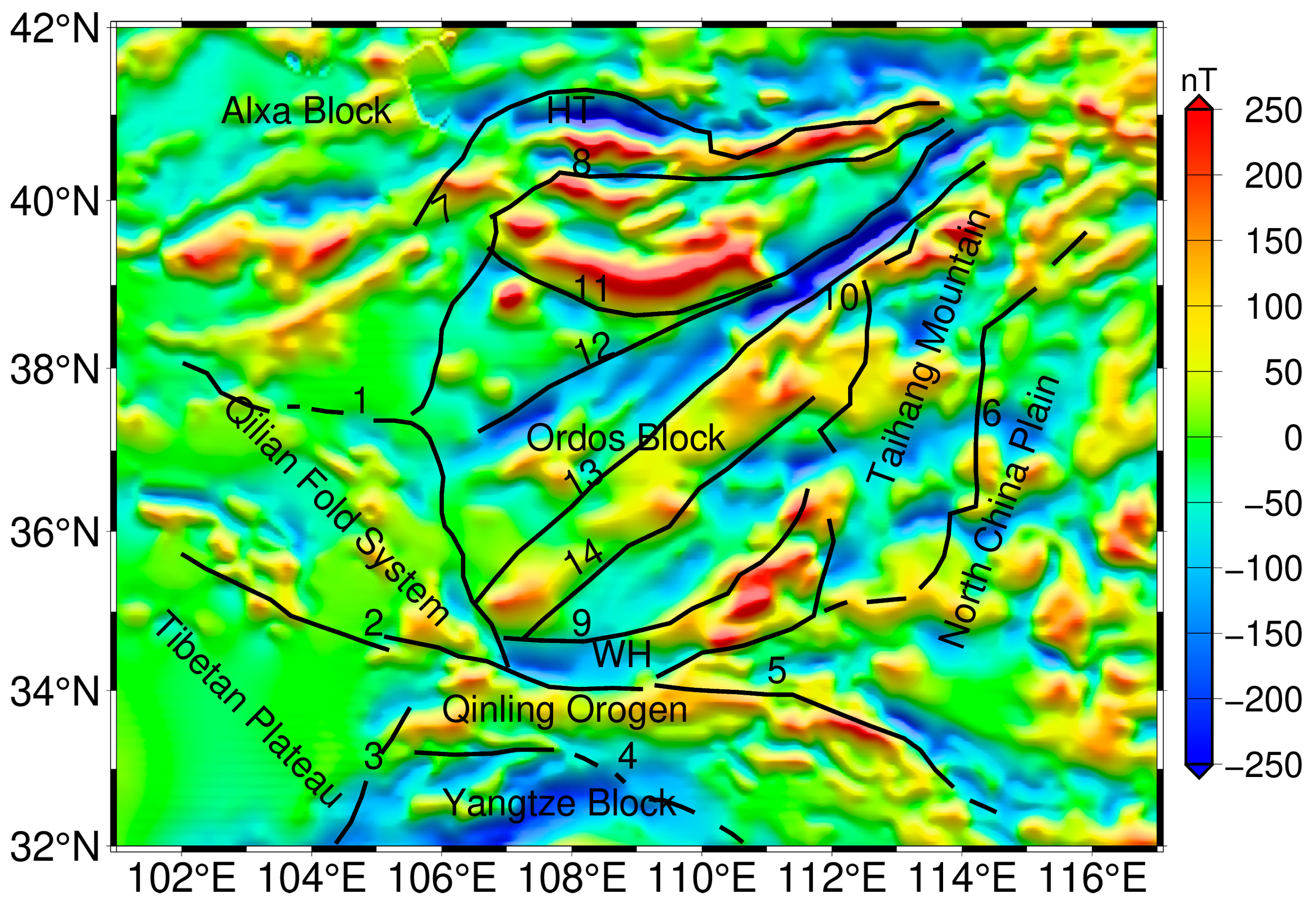
Figure 2.
The measured distribution of heat flow in Ordos and its surrounding areas. A–A′ denotes the profile used in the subsequent analysis.
Figure 2.
The measured distribution of heat flow in Ordos and its surrounding areas. A–A′ denotes the profile used in the subsequent analysis.
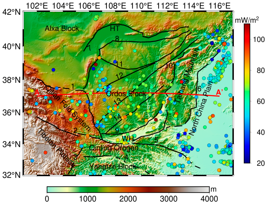
Figure 3.
Synthetic CIS inversion results and error distributions. (a) Synthetic magnetic anomaly field; (b) true synthetic Curie isotherm depth; (c), (e), (g), and (i) inversion results obtained by the traditional method, M1, M2, and M3, respectively; (d), (f), (h), and (j) corresponding absolute error distributions.
Figure 3.
Synthetic CIS inversion results and error distributions. (a) Synthetic magnetic anomaly field; (b) true synthetic Curie isotherm depth; (c), (e), (g), and (i) inversion results obtained by the traditional method, M1, M2, and M3, respectively; (d), (f), (h), and (j) corresponding absolute error distributions.
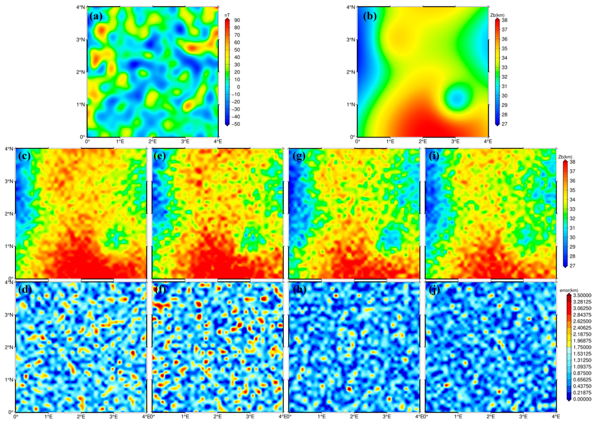
Figure 4.
Synthetic CIS inversion results and error distributions.
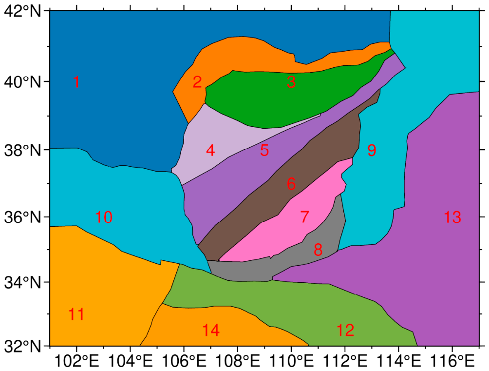
Figure 5.
Bayesian optimized adaptive inversion results in the Ordos Basin and surrounding regions.(a) Curie isotherm surface; (b) moving-window size; (c) fractal index; (d) uncertainty of Curie isotherm surface; (e) representative low-wavenumber fitting for centroid depth Z0; (f) representative medium-to-high-wavenumber fitting for top depth Zt.
Figure 5.
Bayesian optimized adaptive inversion results in the Ordos Basin and surrounding regions.(a) Curie isotherm surface; (b) moving-window size; (c) fractal index; (d) uncertainty of Curie isotherm surface; (e) representative low-wavenumber fitting for centroid depth Z0; (f) representative medium-to-high-wavenumber fitting for top depth Zt.
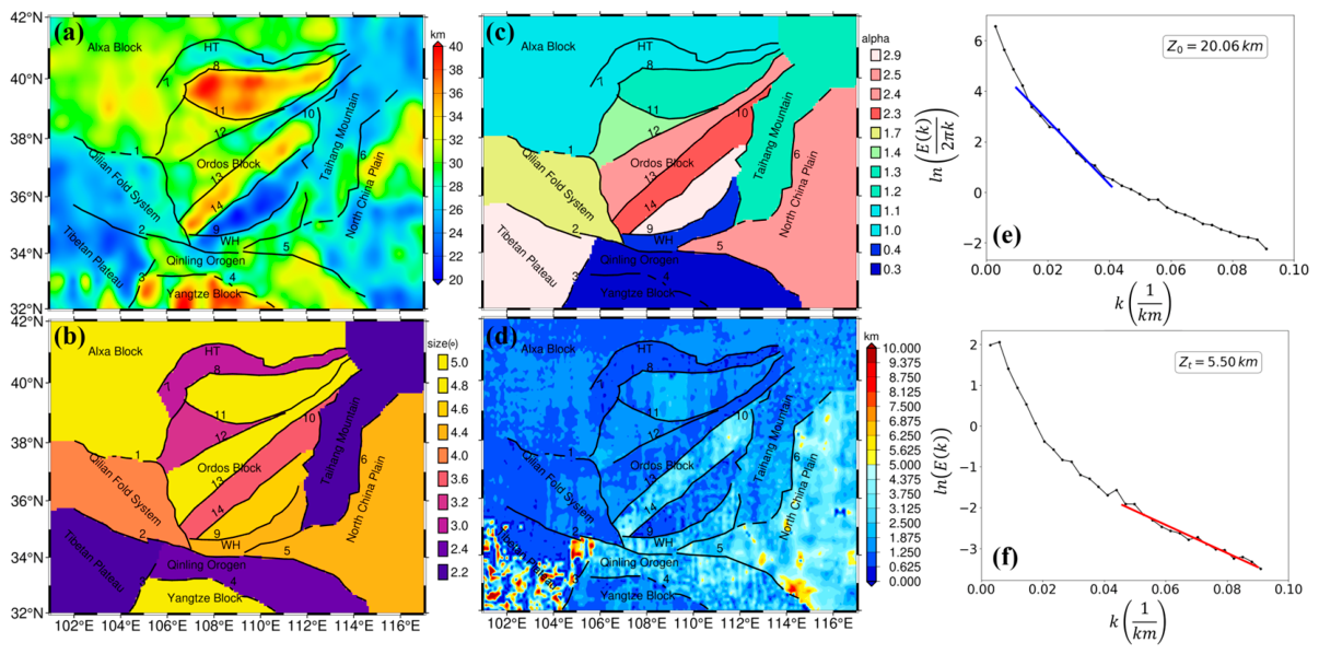
Figure 6.
CIS distributions obtained from three previous studies and this study in the Ordos Basin and surrounding regions.(a) Global reference model of Li et al. (2017); (b) continual-model inversion result of Gao et al. (2015); (c) adaptive-window result of Zhou et al. (2024); and (d) This Study.
Figure 6.
CIS distributions obtained from three previous studies and this study in the Ordos Basin and surrounding regions.(a) Global reference model of Li et al. (2017); (b) continual-model inversion result of Gao et al. (2015); (c) adaptive-window result of Zhou et al. (2024); and (d) This Study.
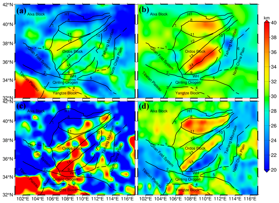
Figure 7.
Comparison of the CIS result obtained in this study with those of three previous studies, together with Moho depth, Bouguer gravity anomaly, and topography along the 37°N profile(A-A’).
Figure 7.
Comparison of the CIS result obtained in this study with those of three previous studies, together with Moho depth, Bouguer gravity anomaly, and topography along the 37°N profile(A-A’).
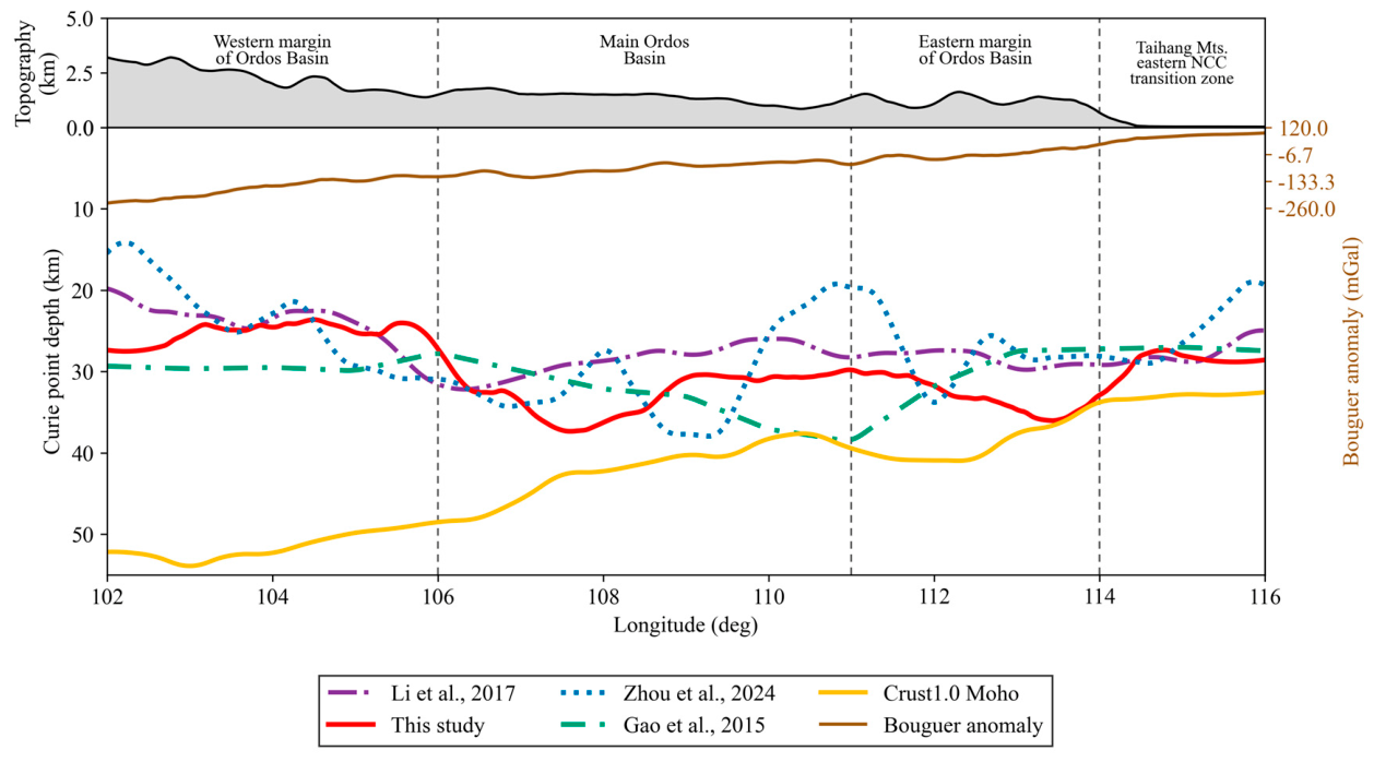
Figure 8.
Crustal structure and Bouguer gravity anomaly distributions in the Ordos Basin and surrounding regions. (a) Bouguer gravity anomaly; (b) Moho depth; (c) upper-middle crustal thickness; (d) total crustal thickness.
Figure 8.
Crustal structure and Bouguer gravity anomaly distributions in the Ordos Basin and surrounding regions. (a) Bouguer gravity anomaly; (b) Moho depth; (c) upper-middle crustal thickness; (d) total crustal thickness.
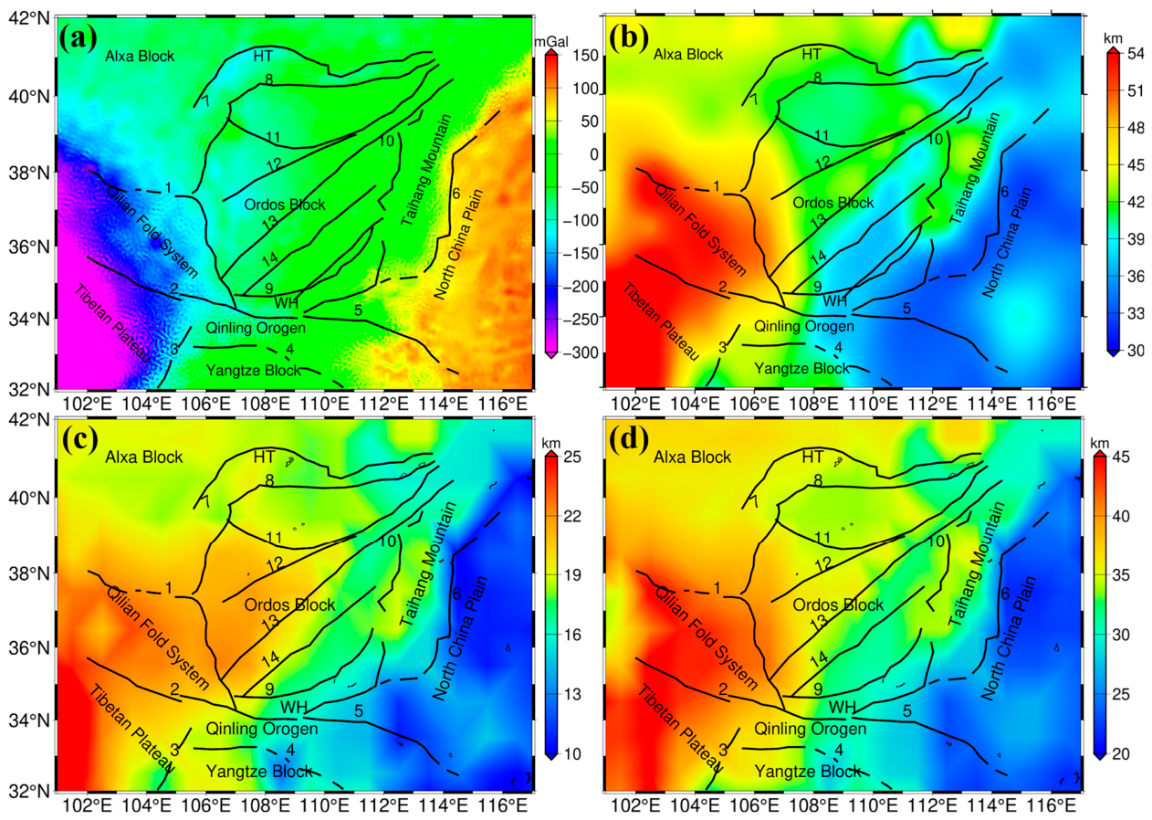
Figure 9.
Conceptual geodynamic model along the A-A’ profile across the northeastern Tibetan Plateau, Ordos Basin, Shanxi Rift System, and North China Plain.
Figure 9.
Conceptual geodynamic model along the A-A’ profile across the northeastern Tibetan Plateau, Ordos Basin, Shanxi Rift System, and North China Plain.
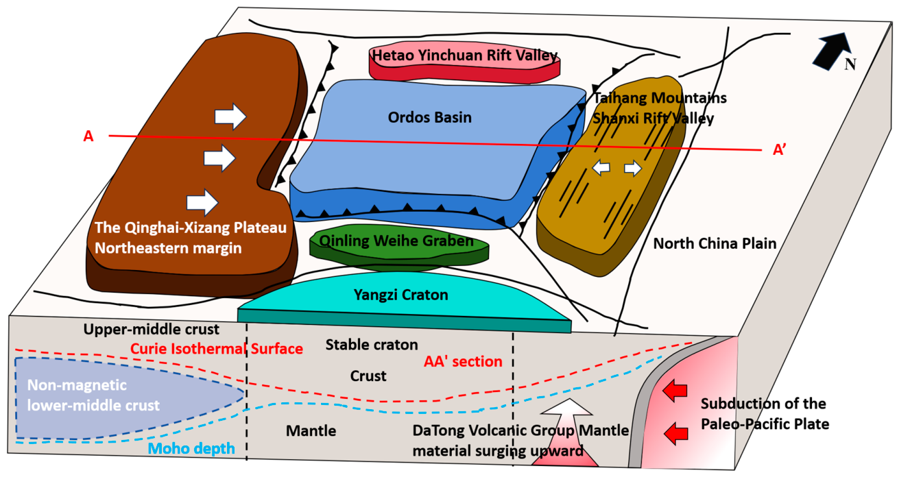
Figure 10.
Spatial distribution of CIS terrestrial heat flow and earthquakes with M≥3.0 from 1900 in the Ordos Basin and surrounding regions.
Figure 10.
Spatial distribution of CIS terrestrial heat flow and earthquakes with M≥3.0 from 1900 in the Ordos Basin and surrounding regions.
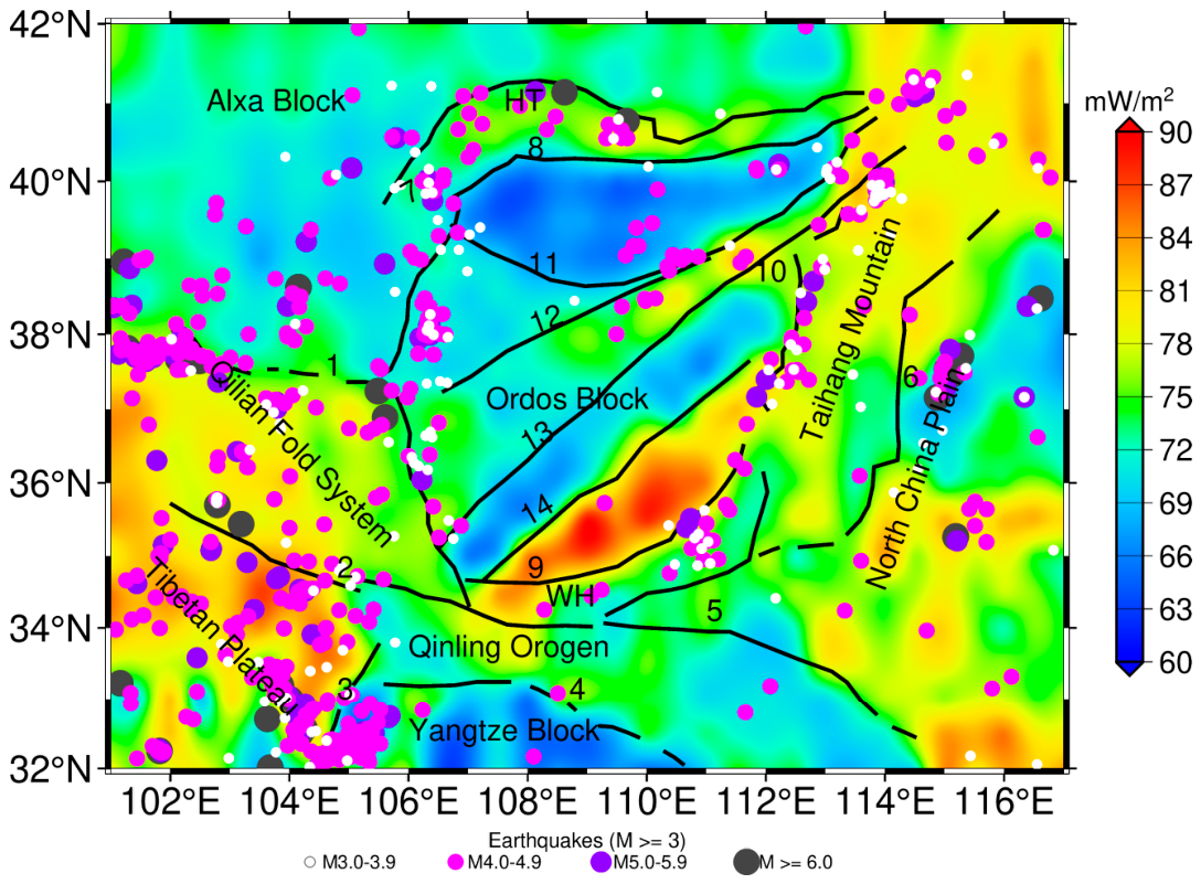

Table 1.
Search ranges and optimal values of the objective-function constraint weights.
| Parameter category | Parameter | Search range | Optimal value |
|---|---|---|---|
| Magnetic-anomaly prior constraint term Lg | Magnetic-anomaly prior weight λg | 0.00-1.20 | 0.30 |
| Prior absolute-deviation weights ηupper and ηdeep | 0.05-0.40 | 0.40 | |
| Lower bound of reliability weight ωmin | 0.05-0.35 | 0.15 | |
| Heat-flow-derived CIS fitting term Lp | Overall weight λp | 0-2 | 1.00 |
| Spatial-distribution constraint term Ls | Spatial-constraint weight λs | 0.20-1.40 | 1.00 |
| Pairwise-difference subterm weight γ1 | 0.20-1.20 | 0.80 | |
| Correlation subterm weight γ2 | 0.40-2.00 | 0.40 | |
| Relative depth-ordering subterm weight γ3 | 0.20-1.40 | 0.50 | |
| Uncertainty constraint term Lu | Mean-uncertainty weight λu,1 | 0.00-0.15 | 0.14 |
| Penalty weight above the preferred threshold λu,2 | 0.00-0.50 | 0.20 | |
| Penalty weight above the soft threshold λu,3 | 0.00-1.20 | 0.40 | |
| Valid-point coverage penalty term Lm | Coverage penalty weight λm | 5-40 | 20 |
Table 2.
Synthetic test experiment results.
| Test method | Traditional method | M1 | M2 | M3 |
| α | 1 | 1 | 1.2 | 1.2 |
| window_size | 3 | 3 | 3.5 | 4 |
| [kt1, kt2] | [0.030, 0.080] | [0.059, 0.089] | [0.044, 0.082] | [0.045, 0.079] |
| [k01, k02] | [0.005, 0.055] | [0.011, 0.058] | [0.004, 0.042] | [0.003, 0.044] |
| RMSE | 1.24 | 1.37 | 0.98 | 0.92 |
| MAE | 1.03 | 1.10 | 0.79 | 0.74 |
| Mean error(%) | 3.12 | 3.32 | 2.36 | 2.23 |
| Median error(%) | 2.88 | 2.80 | 1.97 | 1.88 |
Table 3.
Heat-flow consistency metrics for four CIS models.
| Method/Metric | Gao (2015) | Li (2017) | Zhou (2024) | This Study |
| RMSE (mW/m²) | 34.99 | 46.60 | 54.39 | 35.91 |
| MAE (mW/m²) | 31.36 | 42.86 | 48.57 | 32.46 |
| Corr | 0.05 | 0.20 | 0.10 | 0.19 |
Disclaimer/Publisher’s Note: The statements, opinions and data contained in all publications are solely those of the individual author(s) and contributor(s) and not of MDPI and/or the editor(s). MDPI and/or the editor(s) disclaim responsibility for any injury to people or property resulting from any ideas, methods, instructions or products referred to in the content. |
© 2026 by the authors. Licensee MDPI, Basel, Switzerland. This article is an open access article distributed under the terms and conditions of the Creative Commons Attribution (CC BY) license (http://creativecommons.org/licenses/by/4.0/).
Copyright: This open access article is published under a Creative Commons CC BY 4.0 license, which permit the free download, distribution, and reuse, provided that the author and preprint are cited in any reuse.