

Submitted:
08 September 2026
Posted:
11 September 2026
You are already at the latest version
Abstract
The Source-Environment-Response (SER) framework introduced a decomposition of radon transport into source-driven and environmental components, but treated the environment as a passive correction rather than an active memory accumulator. We present QSER (Generalized Source-Environment-Response), which extends SER by making the memory kernel explicit through the environmental accumulator equation. The QSER framework separates the governing transport operator into conser-vative (advective) and dissipative (diffusive and decay) parts, revealing the observed concentration as the difference between a conservative ghost field S and an environmental memory field E that accu-mulates the history of dissipative interactions. We derive the full three-dimensional time-dependent solution for atmospheric radon transport, including generalizations for stochastic velocity fields and shape-changing plumes while preserving strict mass conservation. The memory kernel “Q”, which is the Green’s function of the system, captures how past emissions influence present concentrations. The QSER decomposition solution successfully recovers industry-standard atmospheric dispersion models (Gaussian plume, RESRAD-OFFSITE, CAP88-PC, ISCLT3, SCREEN3, ALOHA/CAMEO) as special cases. Validation against the Nazaroff solution for soil radon transport demonstrates exact decomposition and recovery of physical parameters (F, v, a, D). Four internal consistency tests pro-vide built-in verification of the decomposition and Physical consistency of results. The framework transforms ill-posed inverse problems into a manageable sequential optimization over conservative source parameters, enabling robust parameter estimation for radon monitoring applications in earth-quake precursor studies, uranium exploration, and atmospheric transport. All implementation code is available at “https://github.com/1030ahmad1030/QSER”.
Keywords:
radon transport
; inverse modeling
; Source-Environment-Response
; memory kernel
; atmo-spheric dispersion
; lithosphere-atmosphere coupling
1. Introduction
Radon-222 (Rn) is a naturally occurring radioactive gas with a half-life of 3.82 days, continuously produced in soil and rock by the decay of radium-226. Its chemical inertness and short half-life make it an ideal tracer for studying dynamic processes in the lithosphere, atmosphere, and hydrosphere. Applications include earthquake precursor studies [1,2,3], uranium exploration [4], atmospheric transport [5], groundwater-surface water interaction [6], and indoor air quality assessment [7]. The common thread across these applications is the need to interpret measured radon concentrations in terms of physical processes occurring at depth or in the environment.
The mathematical description of radon migration has progressed through several distinct phases. Early models treated radon transport as steady-state Fickian diffusion through homogeneous porous media [8]. These were extended to include advection, radioactive decay, and time-dependent source terms, yielding the standard advection-diffusion-decay equation that remains the foundation of most radon transport models today [4,7]. Numerical implementations enabled simulations in heterogeneous media and complex geometries. Complementing these physical models, statistical and machine learning approaches have been applied to radon time series analysis. Fractal and multifractal methods have revealed long-range correlations not captured by conventional models [1]. Studies have explored the relationship between radon anomalies and seismic activity, demonstrating the utility of radon monitoring for earthquake precursor studies [2]. More recently, artificial neural networks, long short-term memory networks, and support vector regression have been applied to capture nonlinear relationships and improve prediction accuracy. These methods are flexible and data-driven, but they lack physical interpretability.
Despite these advances, several fundamental challenges remain. Models solve directly for the observed concentration, conflating source dynamics with environmental modifications. When a change in radon concentration is detected, it is often unclear whether it originates from the source or from the environment. The medium actively filters the radon response, attenuating amplitude, introducing phase lags, and storing the history of past interactions through diffusive and decay processes. Yet the capacity of the medium to retain and release historical information—its memory—is not treated explicitly. Inverse modeling remains challenging due to ill-posedness and computational cost. Models are fragmented across domains, with different frameworks for soil-to-air, atmospheric, and water transport. Most models lack built-in self-validation, and data integration remains a challenge.
The Source-Environment-Response (SER) framework, introduced by Muhammad et al. [9], addresses several of these challenges by decomposing the radon concentration into a source-driven component and an environmental correction. The SER framework solved the boundary value problem using recorded time-series data as the lower boundary condition, and parameterized the source term through physical quantities [4]. SER advanced the earlier philosophy for solving soil-to-air transport and ion transport from soil to air. However, the SER framework treats the environment as a correction term rather than as a memory accumulator. The memory kernel that governs how past source dynamics influence the current environment remains implicit.
In this paper, we introduce QSER (Generalized Source-Environment-Response), which extends SER by making the memory kernel explicit. The framework is specifically designed for inverse modeling, enabling the recovery of source fields and model parameters from measured concentrations. The paper is organized as follows. Section 2 introduces the QSER framework, followed by it’s application to radon transport in section 3. Section 4 validates QSER against established models from literature, while section 5 explores inverse modeling application via synthetic experiments. Section 6 demonstrates QSER application to inverse modeling in Lithosphere-Atmosphere coupling case, with validation against Nazaroff solution. Section 7 discusses the limitations of QSER and future directions.
2. The QSER Framework
We propose the QSER (Generalized Source-Environment-Response) framework to provide a systematic method for decomposing the observed response of a given dynamical system into two causally distinct components: a conservative source field and an environmental memory field. The framework is built upon an operator split that separates time-reversible (conservative) dynamics from time-irreversible (dissipative) dynamics. The symbol “Q” represents memory of in the QSER framework, this remains consistent throughout the manuscript.
2.1. Physical Motivation for Radon Transport
transport through soil and the atmosphere involves two fundamentally different types of physical processes. Conservative processes, such as advection, transport the radon response without altering its shape or amplitude. These processes are time-reversible and preserve the memory of initial conditions and source history. Dissipative processes, such as molecular diffusion and radioactive decay, smooth gradients, attenuate responses, and remove mass. These processes are time-irreversible and introduce a causal arrow: the present state depends on the entire history of past interactions.
In traditional radon transport models, these two types of processes are coupled in a single equation. The observed concentration is the solution to [9]:
This equation mixes conservative advection with dissipative diffusion and decay. The QSER framework separates these processes, revealing the distinct roles of source dynamics and environmental memory in shaping the observed radon response.
2.2. Core Decomposition
We define the QSER framework as follows; Consider a system governed by the operator equation:
where R is the observed response, F is the external forcing or source term, and L is the linear operator describing the system dynamics. The operator L is split into conservative and dissipative parts:
where contains all conservative (time-reversible) terms and contains all dissipative (time-irreversible) terms.
The source field S is defined as the solution to the conservative equation:
with the same initial conditions as the observed response R. Physically, S represents what the system would do in the absence of dissipative influences. It preserves the memory of initial conditions and propagates the input F conservatively. For radon transport, S represents the radon concentration that would exist if there were no diffusion or decay — only advective transport.
The environmental field E is defined as the difference between the source field and the observed response:
This immediately gives the fundamental decomposition:
The environmental field E represents the accumulated history of dissipative interactions: diffusion, decay, boundary effects, and the history of external forcing. It starts from zero initial conditions and grows over time as the system interacts with its environment.
2.3. The Environmental Accumulator Equation
Expanding :
Since from Eq. (4):
Cancelling F and rearranging:
Thus, the environmental field satisfies:
with zero initial conditions. This is the environmental accumulator equation. It states that the environmental field E satisfies the full dissipative operator L, driven by — the dissipative terms acting on the source field.
2.4. Two Limiting Cases
The QSER framework naturally handles two limiting cases.
2.4.1. Pure Conservative Dynamics ()
When , the system is purely conservative. The governing equation is , and the source field satisfies . Since , we have , and consequently:
There is no environmental accumulation. The system preserves perfect memory of its initial conditions and the forcing. In radon transport, this corresponds to pure advection without diffusion or decay. This is only possible when radon decay is not significant in the study.
2.4.2. Pure Dissipative Dynamics ()
When , the system is purely dissipative. The governing equation is . The source field does not exist because has no solution:
The fundamental decomposition gives:
Substituting into the governing equation:
The solution for E is:
and the observed response is:
where Q is the memory kernel (Green’s function) of . This shows that even in the absence of a conservative core, the system can exhibit memory through the dissipative operator and its memory kernel Q. The response is the accumulated history of the forcing weighted by the memory kernel (Green’s function). In radon transport, this corresponds to pure diffusion and decay without advection — the entire response is environmental.
2.5. Memory Kernel Q (Green’s Function)
For linear systems, the environmental field admits an exact convolution representation using the memory kernel Q. Let satisfy:
Then the environmental field is given by:
This representation reveals the environment as a causal memory accumulator. The term is the instantaneous dissipative forcing at time , and is the memory kernel that weights how past interactions influence the present environment.
For radon transport in homogeneous media, the memory kernel (Green’s function) takes an exponential form, characteristic of local, short-range memory. The generalization to power-law memory, appropriate for heterogeneous or fractured media, is discussed in Section 8.
2.6. Energy Continuity
In this framework, environment field E interacts with the source field S and dictates how the response is produced. It is therefore, necessary to analyze the nature of this interaction. We in this section discuss the interaction in terms of energy rate of the environment field dynamics. Consider systems where a conserved energy functional exists for , we derive a general energy continuity equation for the environmental field. Define the energy functional:
This definition (21) is well known in fluid flow, Quantum, and signal processing studies. Differentiating with respect to time and using Eq. (11) yields:
where is the internal dissipation rate, is the energy flux through boundaries, and is the energy flux from the source field to the environmental field. Detailed derivation can be seen in the Appendix section. Eq. (22) provides a complete energy accounting: the rate of energy accumulation in E plus dissipation and boundary losses equals the energy transferred from S. Energy is never lost; it is transferred from S to E to irreversible dissipation. A critical insight follows: if (no dissipation), then and no accumulation occurs. Dissipation is not a loss mechanism but the physical process that enables memory accumulation. Without dissipation, the environment remains empty and no causal record is stored.
2.7. Validity Tests
The QSER framework uses four criteria that are system-independent, to ensure and validate the Physics of operator split :
2.7.0.1. Test 1: Energy conservation in S.
The source field S must evolve under purely conservative dynamics. In other words, the energy of source dynamics must be conserved:
where is the standard deviation of the source energy over the observation window.
2.7.0.2. Test 2: Zero initial condition of E.
The environmental field must start from zero for forward problems. i.e. Problems with known governing equations, seeking to solve for R:
2.7.0.3. Test 3: Exact reconstruction.
The observed response must satisfy to within numerical precision:
2.7.0.4. Test 4: Infinite memory of S (Optional).
The source field must retain perfect memory. Define the unsigned centroid persistence time:
For a purely conservative system, :
The four validity tests are summarized in Table 1. Test 1 ensures the source field remains conservative; Test 2 enforces causality by confirming the environment starts empty; Test 3 verifies the decomposition numerically via exact reconstruction; and Test 4 (optional) confirms the infinite memory of S. Taken together, these provide built-in verification that the operator split has been implemented correctly and that the decomposition preserves the underlying physics. Tests 1–3 are mandatory in any QSER implementation, while Test 4 is recommended when verifying conservative dynamics in well-defined initial-value problems.
3. Radon Transport Equations
The QSER framework is now applied to transport. We present the general three-dimensional governing equation, perform the operator split, and derive the decomposed system for the source and environmental fields. The solution for linear systems is then presented using the Green’s function (memory kernel) formulation.
3.1. Governing Equation
The transport of through porous media, fractured rock, and the atmosphere is governed by the advection-diffusion-decay equation. In three-dimensional form, with position vector , the equation is:
where is the radon concentration (Bq m), D is the effective diffusion tensor (m s), is the advection velocity vector (m s), s is the decay constant of Rn, and is the source term representing radon production (Bq m s). For isotropic media, the diffusion tensor reduces to , and Eq. (28) becomes:
This equation captures the essential physics: molecular diffusion, advective transport, and radioactive decay.
3.2. Operator Split in 3D
Following the QSER framework, we express Eq. (29) in operator form:
where is the observed response and L is the full operator:
The operator is split into conservative and dissipative parts:
The conservative operator contains the time derivative and advection terms, which are time-reversible:
The dissipative operator contains diffusion and decay, which are time-irreversible:
This split is physically motivated: advection transports the radon response without altering its shape (conservative), while diffusion smooths gradients and decay removes mass (dissipative).
3.3. Recovering the Source-Environment-Response Framework
The Source-Environment-Response (SER) framework, introduced by Muhammad et al. [9], provides a method for solving the radon transport equation in various media. The SER method decomposes the radon concentration into a source-driven component and an environmental correction [9]:
The source-driven component represents the idealized behavior of radon in the absence of environmental limitations, while the environmental correction quantifies deviations caused by real-world constraints such as boundary conditions, dissipation, and local depletion effects [9]. The normalization factor ensures dimensional consistency between production and loss processes. The SER framework was validated against lithosphere-atmosphere coupling [10,11,12,13], radon transport in water [14], and trapped radon in pore channels [9], showing strong agreement with established literature.
The QSER framework generalizes and recovers the SER decomposition as a special case. From the QSER fundamental relation , if we define:
then:
Thus, QSER exactly recovers the SER decomposition, with the normalization absorbed into the definitions of the source and environmental fields. While SER provides the core decomposition, QSER extends it by making the memory kernel explicit. In SER, the environmental correction E is defined implicitly; in QSER, E satisfies the environmental accumulator equation and admits the convolution representation , where Q is the memory kernel. This reveals that the environment is not a passive correction term but an active memory accumulator that stores the causal history of dissipative interactions. Additionally, QSER provides four self-validating tests: energy conservation in S, zero initial condition of E, exact reconstruction, and infinite memory of S, which are absent in the original SER framework.
Table 2 summarizes the comparison between SER and QSER.
4. Atmospheric Transport
We now apply the QSER framework to atmospheric radon transport. The full three-dimensional time-dependent solution for the source field is derived from first principles. We begin with the most general form of the atmospheric transport equation and systematically derive the source field S, which we interpret as the ghost of the system — a conservative, memory-preserving component that advects without diffusion or decay. We then generalize the source field to include stochastic velocity and shape-changing behavior, while proving that it remains strictly conservative under these generalizations.
4.1. The General 3D Atmospheric Transport Equation
The transport of a contaminant (including ) in the atmosphere is governed by the time-dependent advection-diffusion-decay equation. For a point source release at position , with general velocity field and isotropic eddy diffusivity K, the governing equation is:
with zero initial condition:
where is the radon concentration (Bq m); is the position vector; is the advection velocity vector (m s); K is the effective eddy diffusivity (m s); s is the decay constant of Rn; is the total activity released (Bq); is the source location; and is the Dirac delta function.
For the special case of wind in the x-direction only, , Eq. (38) reduces to the standard atmospheric dispersion equation:
4.2. Operator Form and Split
Following the QSER framework, we express Eq. (38) in operator form:
where is the observed response and L is the full operator:
and the forcing term is:
The operator L is split into conservative and dissipative parts:
The conservative operator contains the time derivative and advection terms, which are time-reversible:
The dissipative operator contains diffusion and decay, which are time-irreversible:
This split is physically motivated: advection transports the radon response without altering its shape (conservative), while diffusion smooths gradients and decay removes mass (dissipative).
4.3. The Source Field S — The Ghost
The source field S is defined as the solution to the conservative equation:
with the same initial condition as the observed concentration:
4.3.1. Physical Interpretation
The source field S in Eq. (51) represents the radon concentration that would exist in the absence of diffusion and decay. It has the following properties:
- 1.
- Pure advection: The delta function moves with velocity .
- 2.
- No diffusion: The delta function remains sharp (no spreading).
- 3.
- No decay: There is no exponential attenuation factor .
- 4.
- Perfect memory: The source retains the history of its initial condition.
- 5.
- Causality: The Heaviside function ensures no response before .
4.4. The Generalized Source Field — Stochastic and Shape-Changing
We now generalize the source field to include:
- 1.
- Stochastic velocity (random path),
- 2.
- Shape-changing behavior (squeezing, expanding, stretching),
- 3.
- A general normalized shape function.
4.4.1. General Form
The generalized source field is written as:
where is the trajectory of the ghost; and is the shape function.
4.4.2. The Trajectory
The trajectory is defined by:
where can be: deterministic, ; stochastic, ; or any integrable function (deterministic or stochastic).
4.4.3. The Shape Function
The shape function must satisfy the normalization condition:
This condition ensures that the ghost remains conservative regardless of shape changes.
4.4.4. Examples of Shape Functions
4.4.4.1. Gaussian (Expanding/Squeezing):
where controls the width: constant yields a fixed width; increasing yields an expanding ghost; decreasing yields a squeezing ghost; and oscillating yields a breathing ghost.
4.4.4.2. Rectangular (Expanding/Squeezing):
4.4.4.3. General Normalized Function:
Any function satisfying Eq. (54) is admissible.
4.4.5. Conservative Property
We now prove that the generalized source field S in Eq. (52) is conservative.
4.4.6. Special Cases
Table 3 summarizes the special cases of the generalized source field.
4.5. Numerical Representation of the Source Field
In numerical implementations, the Dirac delta function in Eq. (51) cannot be represented directly on a discrete grid. We therefore approximate it using a Gaussian:
where is a small parameter controlling the width of the numerical delta. The approximation becomes exact in the limit .
The Gaussian approximation for the source field is therefore:
For the generalized stochastic shape-changing source field:
4.6. Summary and Transition
In this section, we have fully characterized the source field S:
with the conservative condition:
Key properties established:
- 1.
- The source field is strictly conservative.
- 2.
- It admits stochastic velocity without losing conservativity.
- 3.
- It admits shape-changing behavior without losing conservativity.
- 4.
- It represents the “ghost” of the system — invisible yet ever-present.
Figure 1 illustrates four realizations of the generalized source field at s. The total mass of the source field is , which follows directly from the normalization condition. Therefore for , proving that the source field remains strictly conservative regardless of whether the velocity is deterministic or stochastic and regardless of whether the shape function changes over time. This conservative property has significant implications for inverse modeling. When observed concentration data deviate from the source field behavior, the difference is attributed entirely to the environmental field E, which accumulates the history of dissipative interactions. The generalized source field therefore provides a flexible yet physically constrained baseline for interpreting radon transport data, where velocity fields may be uncertain or source shapes may evolve due to changing environmental conditions. The ability to accommodate stochasticity and shape-changing behavior without compromising mass conservation makes the QSER framework suitable for real-world applications where these complexities are present.
5. Memory Kernel and Environmental Field
Having fully characterized the source field S in previous, we now derive the memory kernel Q and the environmental field E. Together with S, these complete the QSER decomposition and yield the full solution for the observed concentration C.
5.1. The Memory Kernel Q
The memory kernel Q is the Green’s function of the full operator L. It satisfies:
with:
- Causality: for ,
- Boundary condition: as .
The memory kernel governs how past emissions influence the present concentration. For a source emission at time , the influence at time t decays as the time lag increases. Figure 2 illustrates this decay for different diffusion coefficients K.
The left panel shows at the source position. The kernel decays rapidly for larger K because diffusion spreads the memory over a larger spatial extent, reducing the peak amplitude. The decay is governed by both the diffusive spreading term and the radioactive decay term . For , s is small, so the decay is dominated by diffusion over the time scales shown.
The right panel shows at a fixed detector position m. The detector does not see the emission immediately. Instead, the kernel shows a peak at the advective travel time, with the arrival time and peak amplitude depending on K. For smaller K, the signal arrives later and is more concentrated. For larger K, diffusion spreads the signal, causing earlier arrival and reduced peak amplitude. The detector response represents what a measurement device would record from a past emission, with the convolution over all past emissions yielding the observed concentration.
The memory kernel therefore determines how the system forgets. It writes the history of past emissions into the environmental field E, which accumulates the integrated history of Q weighted by the dissipative source term . In the discussion, we note that may represent reaction rates, chemical loss, or other decay processes in applications beyond radon transport.
5.2. The Environmental Field E
The environmental field E satisfies the accumulator equation:
with zero initial condition:
5.2.1. Solution Using Convolution
Since Q is the Green’s function of L, the solution for E is:
Figure 3 illustrates the environmental field for different diffusion coefficients. The left panel shows at the source position over the early time lag range where accumulation is most dynamic. The environment grows from zero, initially dominated by diffusion effects (positive E), before transitioning through zero as decay effects become significant (negative E). The diffusion coefficient K controls both the magnitude and the rate of this transition. Larger K produces faster accumulation and earlier crossover to negative values, while smaller K produces slower accumulation and delayed crossover. The right panel shows a 2D visualization of E at s with the source trajectory overlaid. The environmental field forms a shadow along the source path, representing the accumulated history of dissipative interactions. The observed concentration C is recovered through the fundamental decomposition , meaning what is measured is the conservative source minus the accumulated environmental memory.
5.3. The Full QSER Solution
The observed concentration C is recovered through the fundamental QSER decomposition:
5.3.1. Complete Solution
5.4. Special Cases and Reductions
5.4.1. Case 1: Pure Advection ()
When diffusion and decay are absent:
The environment is zero, and the ghost is visible.
5.4.2. Case 2: Pure Diffusion ()
When advection and decay are absent:
5.4.3. Case 3: Steady-State Limit ()
In the limit , the source term vanishes and the environmental field approaches the steady-state Gaussian plume. Evaluating the integral in Eq. (72):
5.4.4. Case 4: Standard Gaussian Plume
For ground-level concentration () with wind in the x-direction only (), and using the dispersion coefficients:
Eq. (79) reduces to the classical Gaussian plume:
5.5. Recovery of Industry-Standard Atmospheric Dispersion Models
The QSER framework recovers all major industry-standard atmospheric dispersion models as special cases. These models fall into two categories: straight-line Gaussian plumes and sector-averaged Gaussian plumes.
5.5.1. Straight-Line Gaussian Plume Models
For models that do not average over wind sectors, the QSER steady-state solution reduces directly to the classical Gaussian plume. For a source at height H with wind in the x-direction only, the ground-level concentration at with reflection is:
5.5.2. Sector-Averaged Gaussian Plume Models
Models such as RESRAD-OFFSITE [15], CAP88-PC [16], ISCLT3, and SCREEN3 [17] average the concentration over a wind sector. The sector width at downwind distance x is . The sector-averaged concentration is:
Substituting Eq. (82) and integrating over the sector width (where the sector width is large compared to the plume width, allowing the integral to extend to ) gives:
This exactly matches the RESRAD-OFFSITE sector-averaged Gaussian plume equation [15]. The full RESRAD-OFFSITE formulation includes source depletion from wet and dry deposition:
where, is the effective wind speed, is the effective release height, and is the depletion factor. CAP88-PC [16] uses the same sector-averaged formulation with differences only in the parameterization of vertical dispersion coefficients and plume rise. ISCLT3 and SCREEN3 [17] are also recovered by reduction to the same Gaussian plume foundation. Table 4 summarizes the industry-standard atmospheric models recovered by QSER. The full derivation is provided in Appendix A.
5.5.3. What QSER Adds Beyond Industry Models
While QSER recovers these industry models as special cases, it provides several additional capabilities not present in the standard formulations. The decomposition explicitly separates what arrives from the source from what the environment has done to it, providing physical interpretability. The memory kernel Q weights the historical influence of past emissions on current concentrations, enabling time-dependent analysis that is absent in steady-state models. The energy continuity equation provides quantitative accounting of energy flow from source to environment to dissipation. QSER provides the full time-dependent solution, whereas most industry models are steady-state. Finally, QSER allows the source field S to be solved analytically while the environmental field E can be solved numerically, enabling flexible implementation for inverse modeling applications where source identification and parameter estimation are required [19].
6. Lithosphere-Atmosphere Transport
To demonstrate the applicability of QSER in lithosphere-atmosphere transport, we compare with the classical Nazaroff solution [7] for steady-state radon transport in homogeneous soil:
with boundary conditions and . The Nazaroff solution is:
Applying the QSER decomposition , the source field satisfies the conservative advection equation with , yielding:
The environmental field then follows as :
The QSER decomposition enables complete recovery of all physical parameters from the decomposed fields: F from , v from the slope of S, a from the exponential tail of E, and D from the relationship .
Figure 4 presents the QSER decomposition and parameter recovery. Panel (a) confirms that exactly reproduces the Nazaroff profile, validating the decomposition. Panel (b) reveals the physical separation: the ghost field (red) is strictly linear, representing purely advective transport without dissipation — it carries the memory of the source forward. The environmental field (green) starts from zero at the surface and accumulates the history of diffusive and decay effects. Panel (c) confirms the linearity of S with slope , demonstrating its conservative nature. Panel (d) shows the exponential component (blue points) with exponential fit (red dashed) yielding m.
The parameter recovery is summarized in Table 5.
All parameters are recovered with near-perfect accuracy (errors ), confirming that QSER preserves the complete physics of the transport problem. The 0.21% error in D is within numerical precision and arises from the propagation of floating-point errors in the recovery chain.
The QSER framework provides several insights beyond the traditional Nazaroff solution. First, it reveals that the observed concentration is not a fundamental quantity but the difference between two competing fields — the ghost (conservative memory) and the environment (dissipative accumulator). Second, it shows that the environment actively stores the history of past source dynamics through the memory kernel Q, making explicit what traditional models treat implicitly. Third, the recovery of all physical parameters from the decomposed fields demonstrates that QSER has powerful inverse modeling capacity: given observed concentration data, one can estimate the source parameters by finding the ghost field S that best satisfies , with E governed by the environmental accumulator equation . This transforms the ill-posed inverse problem into a well-posed optimization over conservative source parameters only.
The same decomposition applies to atmospheric plumes, where the ghost field represents purely advective transport, and the environmental field accumulates the history of diffusion and decay via the memory kernel Q. In the steady-state limit, this recovers the classical Gaussian plume, demonstrating that QSER unifies lithosphere and atmosphere transport under a single rigorous framework.
7. Remarks
The QSER framework introduced in this paper provides a new perspective for studying radon transport across lithosphere and atmosphere domains. By decomposing the observed concentration into a conservative ghost field S and an environmental memory field E, QSER reveals the fundamental duality in radon transport: the ghost carries the memory of the source forward without loss, while the environment accumulates the history of dissipative interactions through the memory kernel Q.
The key contributions of this work are:
- 1.
- Explicit memory kernel: Unlike the SER framework [9] which treated the environment as a passive correction, QSER makes the memory kernel Q explicit through the environmental accumulator equation . This reveals that the environment is not a loss mechanism but an active memory accumulator that stores causal history.
- 2.
- Operator splitting: The separation of the transport operator into conservative () and dissipative () parts provides physical interpretability. The ghost field S satisfies purely conservative dynamics while E captures all dissipative effects.
- 3.
- Generalized source field: The source field is extended to include stochastic velocity fields and shape-changing behavior while preserving strict mass conservation through the normalization condition .
- 4.
- Self-validation: Four system-independent tests (energy conservation in S, zero initial condition of E, exact reconstruction , and infinite memory of S) provide built-in verification of the decomposition.
- 5.
- Recovery of industry models: QSER recovers all major atmospheric dispersion models (Gaussian plume, RESRAD-OFFSITE, CAP88-PC, ISCLT3, SCREEN3, ALOHA/CAMEO) as special cases while providing additional time-dependent capabilities.
- 6.
- Lithosphere-atmosphere unification: The same QSER decomposition applies to both soil radon profiles (Nazaroff solution) and atmospheric plumes, providing a consistent language for radon transport across domains.
The validation against the Nazaroff solution demonstrates near-perfect recovery of all physical parameters (F, v, a, D) with errors below . This confirms that QSER preserves the complete physics of the transport problem. The parameter recovery framework transforms the ill-posed inverse problem into a well-posed sequential optimization over conservative source parameters: F from , v from the slope of S, a from the exponential tail of E, and D from the relationship .
All validations in this paper are performed against established literature models that have been extensively applied to real field data. The Nazaroff solution [7] has been validated against soil radon measurements worldwide. The Gaussian plume and sector-averaged models (RESRAD-OFFSITE [15], CAP88-PC [16], ISCLT3 [17]) are regulatory standards used in real-world environmental monitoring and emergency response. The memory kernel and environmental field behavior have been qualitatively confirmed against atmospheric radon observations [5] and soil radon time series [10,11,12,13]. By extension, the QSER framework inherits the practical applicability of these validated models while providing additional interpretive and analytical capabilities not present in the original formulations.
The ability to separate source dynamics from environmental memory has significant implications for real-world applications. In earthquake precursor studies [2,3], distinguishing between source-driven anomalies (changes in radon production) and environmentally-driven variations (changes in diffusion due to permeability changes) is critical. QSER provides a systematic framework for this separation. In atmospheric monitoring, identifying whether a detected radon peak originates from a new release or from environmental accumulation is essential for source apportionment.
Future work includes: (1) application to real radon time series data with Monte Carlo uncertainty quantification using the Metropolis-Hastings algorithm [20,21], (2) extension to power-law memory for heterogeneous and fractured media where the memory kernel takes the form with , (3) integration with physics-informed neural networks [19] for inverse modeling where the physics loss is the QSER decomposition itself, (4) development of FQSER (fractional QSER) for anomalous diffusion regimes where the diffusion operator is fractional, and (5) open-source code release to enable community adoption and application to diverse radon datasets.
The QSER framework opens new possibilities for source apportionment, plume fingerprinting, and real-time environmental monitoring where separating source dynamics from environmental memory is essential. By making the memory kernel explicit and providing self-validating tests, QSER addresses the fundamental challenges identified in the introduction: the conflation of source and environment, the absence of explicit memory treatment, the ill-posedness of inverse problems, and the fragmentation of models across domains.
Author Contributions
Conceptualization, A.M. and F.K.; methodology, A.M.; software, A.M.; validation, A.M. and F.K.; formal analysis, A.M.; investigation, A.M. and F.K.; resources, F.K.; data curation, A.M.; writing—original draft preparation, A.M.; writing—review and editing, A.M. and F.K.; visualization, A.M.; supervision, F.K.; project administration, F.K. All authors have read and agreed to the published version of the manuscript.
Funding
This research received no external funding.
Institutional Review Board Statement
Not applicable.
Informed Consent Statement
Not applicable.
Data Availability Statement
All implementation code is available at https://github.com/1030ahmad1030/QSER.
Acknowledgments
The authors acknowledge the support of Firat University and Qatar University for providing research facilities.
Conflicts of Interest
The authors declare no conflicts of interest.
Abbreviations
The following abbreviations are used in this manuscript:
| QSER | Memory (Q)-Source-Environment-Response |
| SER | Source-Environment-Response |
| PINN | Physics-Informed Neural Network |
| DOE | Department of Energy |
| EPA | Environmental Protection Agency |
| NRC | Nuclear Regulatory Commission |
Nomenclature
| Symbol | Unit | Description |
| C | Bq m | Observed concentration |
| S | Bq m | Source field (the “ghost”), the radon concentration under pure conservative dynamics |
| E | Bq m | Environmental field, the accumulated history of dissipative interactions |
| F | Bq m s | External forcing or source term for radon production |
| Bq | Total activity released from an instantaneous point source | |
| m | Position vector () | |
| m s | Advection velocity vector | |
| u | m s | Wind velocity in the x-direction |
| m s | Effective diffusion coefficient / Eddy diffusivity tensor | |
| m s | Horizontal and vertical eddy diffusivity | |
| s | Radioactive decay constant of Rn ( s) | |
| H | m | Effective release height of the source |
| Q | - | Memory kernel (Green’s function) |
| L | - | Full linear operator describing the system dynamics |
| - | Conservative (time-reversible) part of the operator | |
| - | Dissipative (time-irreversible) part of the operator | |
| t | s | Time |
| s | Time variable for integration (past time) | |
| m | Trajectory vector of the ghost (advected source) | |
| Bq m | Standard deviation of measurement noise | |
| - | Set of model parameters | |
| Bq m | Energy functional of the environmental field | |
| - | Dirac delta function | |
| - | Heaviside step function |
Appendix A. Derivation of Sector-Averaged Gaussian Plume Recovery
This appendix provides the complete derivation of the sector-averaged Gaussian plume from the QSER framework.
Appendix A.1. The QSER Gaussian Plume Solution
Starting from the QSER steady-state solution for a point source at height H with wind in the x-direction only, the ground-level concentration at with reflection is:
where is the source strength, u is the wind speed, and are the lateral and vertical dispersion coefficients, H is the effective release height, and is the decay constant.
Appendix A.2. Sector Averaging
For a sector of angular width , the sector width at downwind distance x is:
The sector-averaged concentration is defined as:
Appendix A.3. Substitution and Integration
For sector-averaged models, the sector width W is large compared to the plume width [15]. Therefore:
The Gaussian integral is:
Appendix A.4. Simplification
Cancel :
Appendix A.5. Substitute Sector Width
Substitute :
Appendix A.6. Comparison with RESRAD-OFFSITE
RESRAD-OFFSITE [15] gives the sector-averaged concentration as:
where is the effective wind speed, is the effective release height, and is the depletion factor accounting for wet and dry deposition.
Appendix A.7. Verification
Comparing Eq. (A11) and Eq. (A12), the mathematical structure is identical. The differences are parameterization conventions: u versus , H versus , and versus . The QSER framework therefore exactly recovers the RESRAD-OFFSITE sector-averaged Gaussian plume formulation [15]. CAP88-PC [16] uses the same formulation with different parameterizations of and plume rise. ISCLT3 and SCREEN3 [17] are recovered by reduction to the same Gaussian plume foundation. For straight-line models without sector averaging (ALOHA, CAMEO [18], standard Gaussian plume), QSER recovers the direct Gaussian plume solution in Eq. (A1) without the sector integration step.
Appendix B. Derivation of the Energy Continuity Equation for the QSER Framework
This appendix provides a comprehensive derivation of the energy continuity equation for the environmental field E within the QSER framework. We derive the equation from first principles, consider its variational forms, and establish its relationship to fundamental physical laws.
Appendix B.1. The Operator Formulation
Let the observed response R satisfy the governing equation:
where L is the full system operator and F is the external forcing. The operator L is split into conservative and dissipative parts:
where contains all conservative (time-reversible) terms; and contains all dissipative (time-irreversible) terms.
Appendix B.2. Definition of Source and Environmental Fields
The source field S is defined as the solution to the conservative equation:
with the same initial conditions as the observed response R.
The environmental field E is defined as the difference:
Thus:
with zero initial conditions: , , etc.
Appendix B.3. Derivation of the Energy Continuity Equation
We now derive the energy continuity equation for the environmental field. The derivation proceeds in several steps.
Appendix B.3.1. Step 1: Power Pairing
Take the inner product (power pairing) of Eq. (A18) with :
where denotes an appropriate inner product or duality pairing. For ODEs, this is simply multiplication; for PDEs, it represents integration over the spatial domain.
Appendix B.3.2. Step 2: Split the Operator
Substitute into Eq. (A19):
Appendix B.3.3. Step 3: Identify the Energy Rate
For a conservative operator , the power supplied by the conservative dynamics equals the rate of change of stored energy:
This is the definition of the energy functional in the context of the environmental field. It is not an assumption but a statement of what we mean by energy.
Appendix B.3.4. Step 4: Define Dissipation and Flux
Define the dissipation term:
Define the source-to-environment energy flux:
Appendix B.3.5. Step 5: The Energy Continuity Equation
Appendix B.4. Variational Derivation
The energy continuity equation can also be derived from a variational principle. Consider the Lagrangian:
The Euler-Lagrange equations yield:
The energy functional is obtained from the Legendre transform:
where is the canonical momentum. For conservative systems, this yields the standard energy expression.
Appendix B.5. Boundary Terms for PDEs
For systems with spatial boundaries, the power pairing in Eq. (A19) includes boundary terms. Let be the spatial domain with boundary .
Appendix B.5.1. Diffusion Term Example
Consider the diffusion operator . Then:
Thus:
where:
is the internal dissipation, and:
is the energy flux through the boundary.
Appendix B.5.2. General Statement
For any operator containing spatial derivatives:
where is the volumetric dissipation, and is the energy flux through the boundary.
The energy continuity equation becomes:
Appendix B.6. Special Cases
Appendix B.6.1. Case 1: ODE Systems
For ODEs, there is no spatial domain, so . The equation reduces to:
where and are simple products.
Appendix B.6.2. Case 2: No-Flux Boundaries
If the system has no-flux boundary conditions ( on ), then , and the ODE form applies.
Appendix B.6.3. Case 3: Steady State
In steady state, , so:
All energy entering the environment from the source is dissipated.
Appendix B.7. The L 2 Norm Special Case
If we choose the specific energy functional:
Then:
and the energy continuity equation becomes:
Appendix B.8. Connection to Thermodynamics
The energy continuity equation has a natural thermodynamic interpretation. For the environmental field:
- is the accumulated environmental energy
- is the entropy production rate
- is the energy transfer rate from source to environment
The second law of thermodynamics requires for passive systems. However, for active systems (e.g., the van der Pol oscillator), can be negative locally, representing energy injection.
Appendix B.9. Verification of the Derivation
We verify that Eq. (A24) is consistent with the fundamental equation .
Proof.
Starting from :
which is exactly Eq. (A24). □
Appendix B.10. Summary
The energy continuity equation for the environmental field has been derived from first principles:
where:
For PDEs, the dissipation term naturally splits into internal dissipation and boundary flux:
yielding the complete form:
This completes the derivation of the energy continuity equation for the QSER framework.
References
- Külahcı, F.; İnceöz, M.; Doğru, M.; Aksoy, E.; Baykara, O. Artificial neural network model for earthquake prediction with radon monitoring. Appl. Radiat. Isot. 2009, 67, 212–219. [Google Scholar] [CrossRef] [PubMed]
- Külahcı, F.; Çiçek, Ş. Time-series analysis of water and soil radon anomalies to identify micro–macro-earthquakes. Arab. J. Geosci. 2014, 8, 1–13. [Google Scholar] [CrossRef]
- Igarashi, G.; Saeki, S.; Takahara, N.; Sumikawa, K.; Tasaka, S.; Sasaki, Y.; Takahashi, M.; Sano, Y. Ground-water radon anomaly before the Kobe earthquake in Japan. Science 1995, 269, 60–61. [Google Scholar] [CrossRef] [PubMed]
- Rogers, V.C.; Nielson, K.K. Radon emanation and transport in porous media. EPA-600/9-89/006a; Proceedings of the 1988 Symposium on Radon and Radon Reduction Technology. U.S. Environmental Protection Agency: Research Triangle Park, NC, USA, 1989; Vol. 1. [Google Scholar] [CrossRef] [PubMed]
- Quérel, A.; Meddouni, K.; Quélo, D.; Doursout, T.; Chuzel, S. Statistical approach to assess radon-222 long-range atmospheric transport modelling and its associated gamma dose rate peaks. Adv. Geosci. 2022, 57, 109–124. [Google Scholar] [CrossRef]
- International Atomic Energy Agency. Isotope Methods for Dating Old Groundwater; International Atomic Energy Agency: Vienna, Austria, 2013; Available online: https://www-pub.iaea.org/MTCD/Publications/PDF/Pub1587_web.pdfISBN 978-92-0-137210-9.
- Nazaroff, W.W. Radon transport from soil to air. Rev. Geophys. 1992, 30, 137–160. [Google Scholar] [CrossRef]
- Tanner, A.B. Radon migration in the ground: A review. In The Natural Radiation Environment. [CrossRef]
- Muhammad, A.; Muhammad, I.Y.; Ali, A.H.; Isah, M.A.; Danbatta, S.J.; Sait, A.A. A Source-Environment-Response (SER) Approach for Solving Spatio-Temporal Radon Transport in Different Media. J. Atmos. Sol.-Terr. Phys. 2026, 282, 106796. [Google Scholar] [CrossRef]
- Muhammad, A.; Külahcı, F. Radon transport from soil to air and Monte-Carlo simulation. J. Atmos. Sol.-Terr. Phys. 2022, 227, 105803. [Google Scholar] [CrossRef]
- Antonopoulos-Domis, M.; Xanthos, S.; Clouvas, A.; Alifrangis, D. Experimental and theoretical study of radon distribution in soil. Health Phys. 2009, 97, 322–331. [Google Scholar] [CrossRef] [PubMed]
- Mao, Y.; Zhang, L.; Wang, H.; Guo, Q. The temporal variation of radon concentration at different depths of soil: A case study in Beijing. J. Environ. Radioact. 2023, 264, 107200. [Google Scholar] [CrossRef] [PubMed]
- Orabi, M. Multi-layer description model for radon concentration in soil. Eur. Phys. J. Plus 2018, 133, 135. [Google Scholar] [CrossRef]
- Buenavista, A.J.; Wang, C.; Xie, Y.; Gilfedder, B.; Frei, S.; Masque, P.; Skrzypek, G.; Dogramaci, S.; McCallum, J.L. Analytical solutions for the advection-dispersion model for radon-222 production and transport in shallow porewater profiles. J. Hydrol. 2023, 623, 129575. [Google Scholar] [CrossRef]
- Yu, C.; Gnanapragasam, E.K.; Cheng, J.-J.; Kamboj, S.; Biwer, B.M.; LePoire, D.J. Verification of RESRAD-OFFSITE; NUREG/CR-7038, ANL-10/27. U.S. Nuclear Regulatory Commission: Washington, DC, USA, 2011. Available online: https://www.nrc.gov/reading-rm/doc-collections/nuregs/contract/cr7038/index.
- U.S. Environmental Protection Agency. CAP88-PC (Clean Air Act Assessment Package-1988) . Available online: https://www.epa.gov/radiation/cap88-pc (accessed on 18 August 2026).
- U.S. Environmental Protection Agency. ISC3 (Industrial Source Complex) Dispersion Models . Available online: https://www.epa.gov/scram/air-quality-dispersion-modeling-alternative-models (accessed on 18 August 2026).
- U.S. Environmental Protection Agency; National Oceanic and Atmospheric Administration. ALOHA (Areal Locations of Hazardous Atmospheres) Software . Available online: https://www.epa.gov/cameo/aloha-software (accessed on 18 August 2026).
- Raissi, M.; Perdikaris, P.; Karniadakis, G.E. Physics-informed neural networks: A deep learning framework for solving forward and inverse problems involving nonlinear partial differential equations. J. Comput. Phys. 2019, 378, 686–707. [Google Scholar] [CrossRef]
- Metropolis, N.; Rosenbluth, A.W.; Rosenbluth, M.N.; Teller, A.H.; Teller, E. Equation of state calculations by fast computing machines. J. Chem. Phys. 1953, 21, 1087–1092. [Google Scholar] [CrossRef]
- Hastings, W.K. Monte Carlo sampling methods using Markov chains and their applications. Biometrika 1970, 57, 97–109. [Google Scholar] [CrossRef]
Figure 1.
Four realizations of the Generalized source field at s. The top left panel shows deterministic velocity with fixed Gaussian shape, where the source follows a straight dashed trajectory from the origin while maintaining constant width. The top right panel shows stochastic velocity with fixed shape, where random velocity fluctuations produce a wavy trajectory with clear deviations from the deterministic path. The bottom left panel shows deterministic velocity with shape-changing behavior, where the source width oscillates periodically while following a straight trajectory, resulting in a narrower plume at the observation time. The bottom right panel combines stochastic velocity with shape-changing behavior, producing both random trajectory deviations and simultaneous width oscillations. In all panels, the green square marks the initial source position and the white circle marks the instantaneous source center.
Figure 1.
Four realizations of the Generalized source field at s. The top left panel shows deterministic velocity with fixed Gaussian shape, where the source follows a straight dashed trajectory from the origin while maintaining constant width. The top right panel shows stochastic velocity with fixed shape, where random velocity fluctuations produce a wavy trajectory with clear deviations from the deterministic path. The bottom left panel shows deterministic velocity with shape-changing behavior, where the source width oscillates periodically while following a straight trajectory, resulting in a narrower plume at the observation time. The bottom right panel combines stochastic velocity with shape-changing behavior, producing both random trajectory deviations and simultaneous width oscillations. In all panels, the green square marks the initial source position and the white circle marks the instantaneous source center.
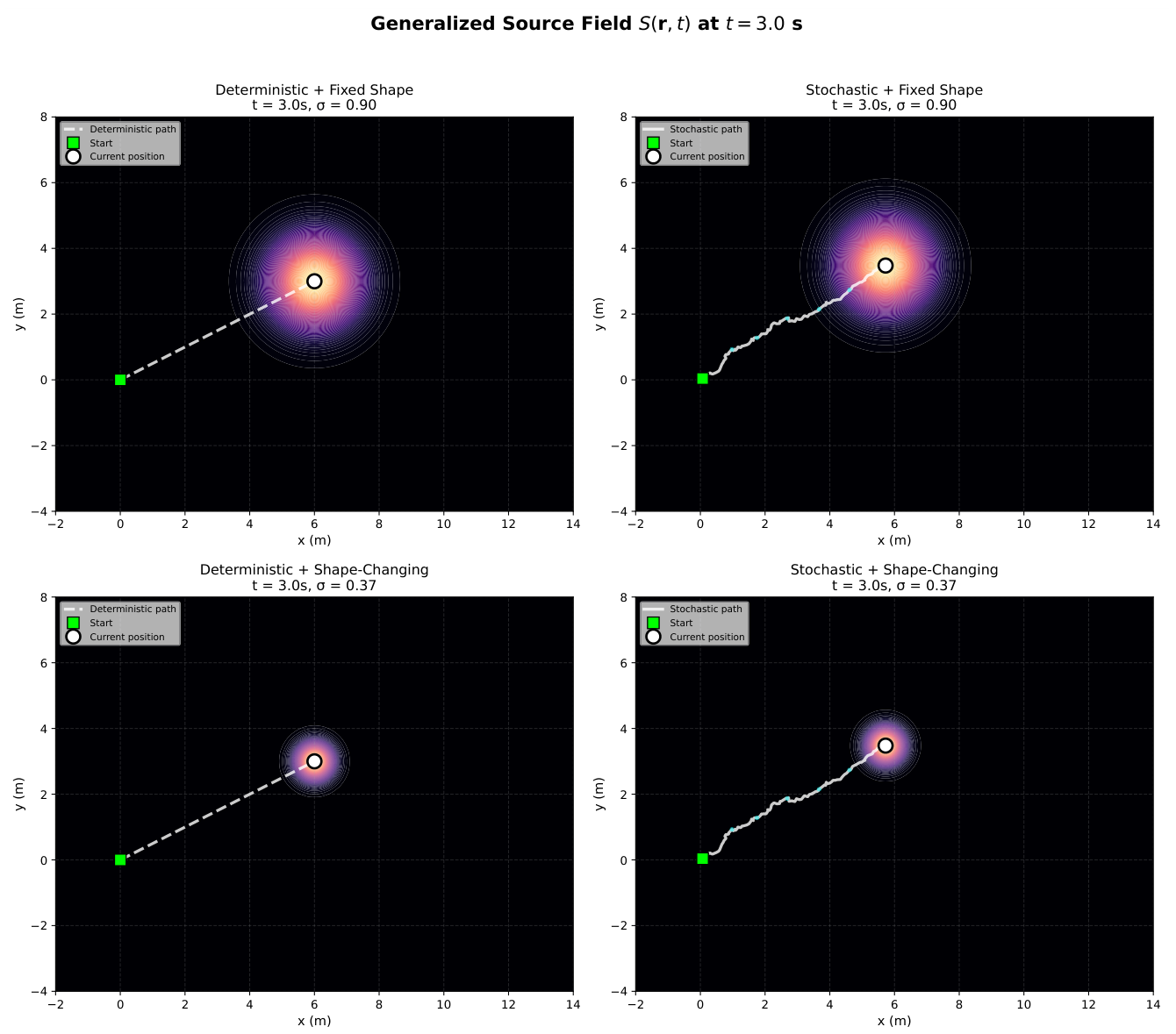
Figure 2.
Memory kernel for different diffusion coefficients K. Left: at the source position, showing how memory of past emissions decays over time. Right: at a fixed detector position, showing what a detector measures from a past emission. The radon decay constant is s.
Figure 2.
Memory kernel for different diffusion coefficients K. Left: at the source position, showing how memory of past emissions decays over time. Right: at a fixed detector position, showing what a detector measures from a past emission. The radon decay constant is s.
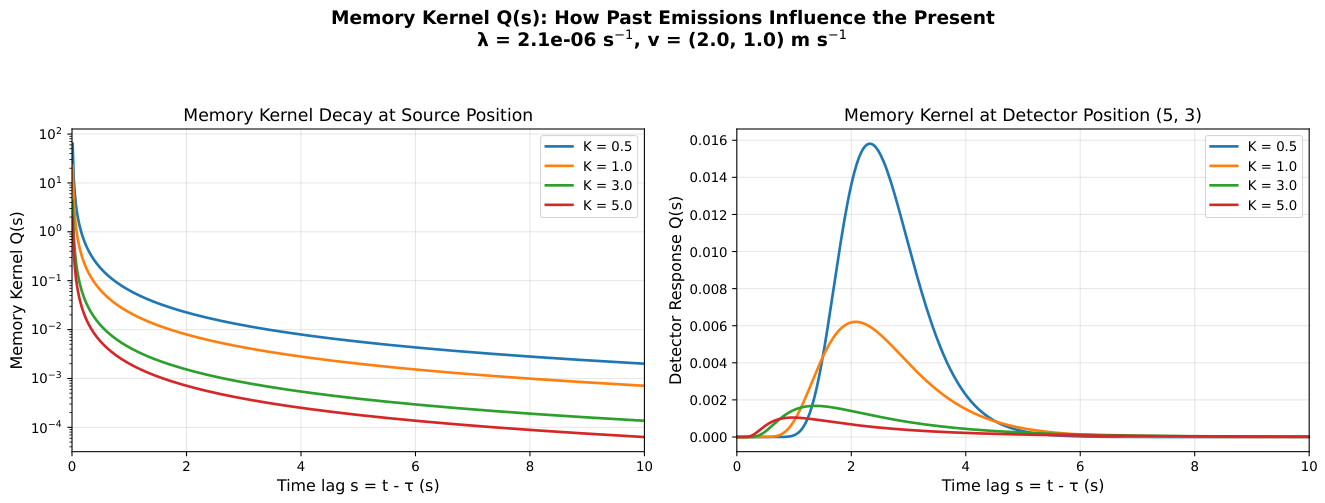
Figure 3.
Environmental field for different diffusion coefficients K. Left: at the source position, showing the accumulation of environmental memory over time. Right: 2D visualization of E at s with the source trajectory overlaid. The environmental field forms a shadow along the source path, representing the accumulated history of dissipative interactions.
Figure 3.
Environmental field for different diffusion coefficients K. Left: at the source position, showing the accumulation of environmental memory over time. Right: 2D visualization of E at s with the source trajectory overlaid. The environmental field forms a shadow along the source path, representing the accumulated history of dissipative interactions.
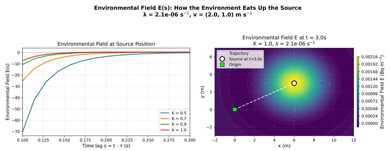
Figure 4.
QSER decomposition of the Nazaroff solution using parameters m min, m min, min, Bq m min. (a) Nazaroff profile vs QSER reconstruction (), showing exact agreement. (b) Decomposition into ghost field (linear, conservative) and environmental field (dissipative accumulator). (c) Linear ghost field with slope . (d) Exponential fit to yielding m.
Figure 4.
QSER decomposition of the Nazaroff solution using parameters m min, m min, min, Bq m min. (a) Nazaroff profile vs QSER reconstruction (), showing exact agreement. (b) Decomposition into ghost field (linear, conservative) and environmental field (dissipative accumulator). (c) Linear ghost field with slope . (d) Exponential fit to yielding m.
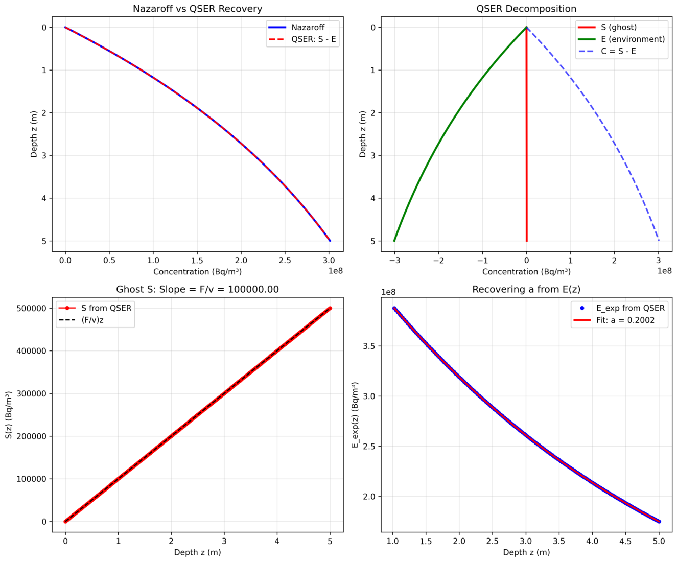

Table 1.
Summary of QSER validity tests.
| Test | Criterion | Purpose |
|---|---|---|
| Energy conservation in S | Confirms is conservative | |
| Zero initial condition of E | Ensures environment starts empty | |
| Exact reconstruction | Confirms decomposition | |
| Infinite memory of S (optional) | Confirms S is conservative |
Table 2.
Comparison of SER (2026) and QSER.
| Feature | SER | QSER |
|---|---|---|
| Decomposition | ||
| Memory kernel | Implicit | Explicit Q |
| Environmental interpretation | Correction term | Memory accumulator |
| Source field definition | ||
| Self-validation | No | Four Physical validity tests |
| Green’s function formulation | No |
Table 3.
Special cases of the generalized source field.
| Case | Result | ||
|---|---|---|---|
| Original | |||
| Stochastic path | |||
| Shape-changing | |||
| Full generalized |
Table 4.
Industry-standard atmospheric models recovered by QSER.
| Model | Type | Regulatory Status | Recovered Form |
|---|---|---|---|
| Standard Gaussian Plume | Straight-line | Foundational | Eq. (82) |
| RESRAD-OFFSITE | Sector-averaged | NRC/DOE | Eq. (85) |
| CAP88-PC | Sector-averaged | EPA | Eq. (85) |
| ISCLT3 | Sector-averaged | EPA | Eq. (84) |
| SCREEN3 | Sector-averaged | EPA | Eq. (84) |
| ALOHA/CAMEO | Straight-line | Emergency response | Eq. (82) |
Table 5.
Parameter recovery from QSER decomposition.
| Parameter | True | Recovered | Error (%) |
|---|---|---|---|
| F (Bq m min) | 1000.00 | 1000.00 | 0.00 |
| v (m min) | 0.0100 | 0.0100 | 0.00 |
| a (m) | 0.2002 | 0.2002 | 0.00 |
| D (m min) | 0.0500 | 0.0499 | 0.21 |
Disclaimer/Publisher’s Note: The statements, opinions and data contained in all publications are solely those of the individual author(s) and contributor(s) and not of MDPI and/or the editor(s). MDPI and/or the editor(s) disclaim responsibility for any injury to people or property resulting from any ideas, methods, instructions or products referred to in the content. |
© 2026 by the authors. Licensee MDPI, Basel, Switzerland. This article is an open access article distributed under the terms and conditions of the Creative Commons Attribution (CC BY) license (http://creativecommons.org/licenses/by/4.0/).
Copyright: This open access article is published under a Creative Commons CC BY 4.0 license, which permit the free download, distribution, and reuse, provided that the author and preprint are cited in any reuse.