

Submitted:
09 September 2026
Posted:
10 September 2026
You are already at the latest version
Abstract
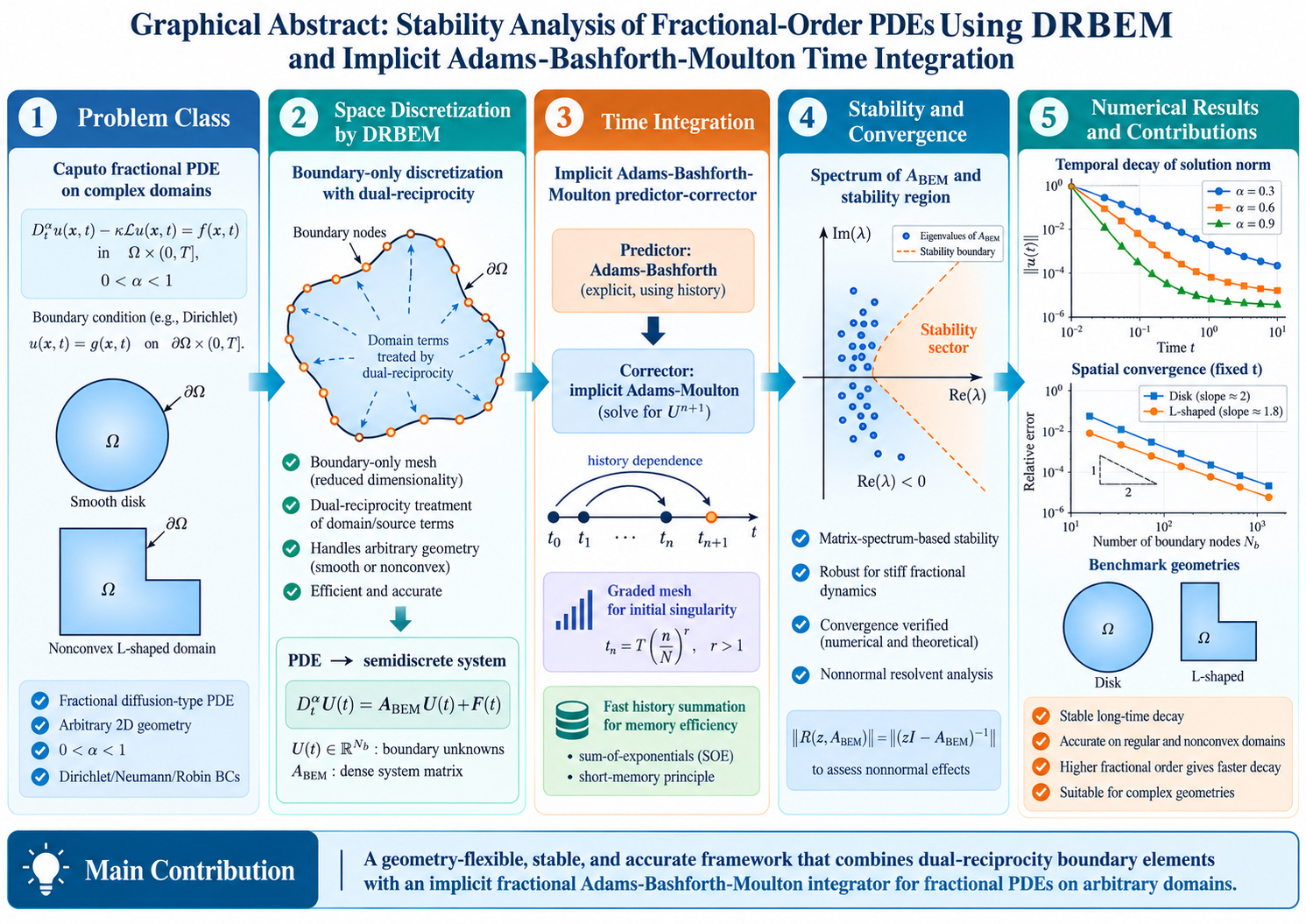
A geometry-aware and stiffness-robust boundary element framework is developed for time-fractional partial differential equations governed by hereditary diffusion, reaction, and transport mechanisms. The formulation couples dual-reciprocity boundary reduction with an Adams predictor and an implicit Moulton correction in which the stiff diffusive boundary element operator is retained at the new time level. This construction moves stability assessment from an isolated scalar test equation to the spectrum, numerical range, and resolvent behavior of the assembled spatial operator, so that geometry, boundary conditions, collocation nonnormality, and stiffness enter the analysis directly. A graded start-up strategy addresses the loss of temporal regularity associated with fractional memory, while compressed history evaluation provides a scalable route for long-time simulations. The theoretical development establishes modal and resolvent-based stability conditions, consistency and convergence properties, and a practical post-assembly stability certificate. Verification on smooth curved and nonconvex domains demonstrates accurate boundary-reduced spatial approximation, robust temporal convergence, resistance to diffusion-driven stiffness, and reliable evolution in the presence of corner singularities. The resulting framework provides a unified and extensible computational architecture for fractional diffusion, reaction transport, thermal memory, and related multiphysics models in geometries for which global spectral discretizations are restrictive.
Keywords:
fractional partial differential equation
; Caputo derivative
; boundary element method
; dual reciprocity
; Adams-Bashforth-Moulton
; predictor-corrector
; stability
; anomalous diffusion
; complex geometry
1. Introduction
Fractional partial differential equations have become a mature modeling paradigm for anomalous diffusion, hereditary transport, relaxation, thermal memory, viscoelastic response, porous-media dynamics, and multiscale processes in which the present state depends on a nonlocal temporal history. Their numerical solution is substantially more demanding than that of classical parabolic equations because every new time level is coupled to the entire preceding trajectory and because the exact solution commonly possesses limited regularity near the initial state. The space-spectral time Adams–Bashforth–Moulton formulation of Sohail, Maqbool, and Ellahi provided an important stability-oriented reference for fractional partial differential equations [1]. The modern fractional Adams methodology is supported by detailed predictor–corrector error analysis [2], stability results for fractional Adams–Moulton formulas [3], and explicit characterization of predictor–corrector stability regions [4]. Graded-mesh analysis has clarified the order degradation induced by weak initial singularities [5], while fast high-order predictor–corrector constructions have demonstrated that graded temporal resolution and compressed memory can be combined without abandoning the Adams framework [6]. These developments establish a strong temporal foundation, but they do not by themselves resolve the interaction between fractional time integration and a stiff spatial operator generated on a geometrically complex domain.
For irregular, multiply connected, curved, or nonconvex domains, global spectral collocation may become restrictive because geometric mappings, global basis construction, and boundary-condition enforcement can dominate the numerical design. Boundary element methods offer a fundamentally different spatial architecture by concentrating geometric discretization on the boundary while retaining direct access to boundary fluxes and interior reconstruction. The dual-reciprocity formulation of Wrobel and Brebbia transformed nonhomogeneous diffusion terms into boundary quantities [7], and early nonlinear transient applications showed that the same mechanism could accommodate strongly coupled thermal source terms [8]. More recent fractional boundary element developments have treated Caputo anomalous diffusion directly [9], extended boundary integral formulations to fractional diffusion-wave dynamics [10], and combined boundary reduction with global temporal algebra for multiorder advection–diffusion–reaction equations [11]. Collectively, these studies demonstrate the geometric flexibility of boundary formulations; however, they also expose a decisive methodological question that is often left implicit: the time integrator must be designed for the actual dense and potentially nonnormal evolution operator produced by the boundary discretization.
A second difficulty is the hereditary memory cost. Direct evaluation of the Caputo history produces growing storage and arithmetic burdens as the simulation horizon increases. Sum-of-exponentials acceleration provides a controlled mechanism for reducing this cost while preserving fractional accuracy [12]. At the same time, explicit fractional diffusion schemes can possess stability restrictions that are substantially more severe than their integer-order analogues [13]. Convolution quadrature provides an alternative operator-based route to stable fractional evolution [14], founded on Lubich’s discretized operational calculus [15], while adaptive multidimensional simulations have emphasized the need to balance temporal history resolution against spatial approximation error [16]. The resulting conclusion is structural rather than algorithm-specific: memory, stiffness, and spatial discretization are coupled features of the same fully discrete problem and should therefore be analyzed within one operator-level framework.
Temporal regularity further complicates the design of high-order algorithms. The Alikhanov difference formula provides a widely used stable high-order benchmark for time-fractional diffusion [17]. Sharp graded-mesh analysis quantifies the interaction between start-up singularity and temporal refinement [18], while nonuniform first-order theory [19] and discrete fractional Grönwall inequalities [20] provide powerful stability tools for variable-step discretizations. Earlier fully discrete diffusion-wave analysis [21], finite-difference spectral approximations [22], higher-order Caputo differentiation formulas [23], and time-stepping estimates for nonsmooth initial data [24] all show that formal consistency order is not sufficient to guarantee practical reliability. A credible fractional solver must state its regularity assumptions explicitly, separate smooth compatible verification from generic weakly singular behavior, and provide a mechanism for recovering accuracy when the initial layer is unresolved. The overview of Jin, Lazarov, and Zhou situates these issues within the broader numerical theory of time-fractional evolution equations with nonsmooth data [25].
Transient boundary element research has addressed dense algebra and time marching through several complementary strategies. Matrix inversion can be avoided or reorganized in dual-reciprocity heat conduction [26], precise integration can be applied to the semidiscrete dual-reciprocity system [27], and isogeometric dual reciprocity can preserve exact geometric descriptions while handling transient heat sources [28]. Earlier nonlinear boundary element formulations already demonstrated the effectiveness of time-independent fundamental solutions for transient nonlinear heat conduction [29]. More recently, nonuniform second-order fractional formulas have supplied an additional route for resolving early-time singular behavior without sacrificing asymptotic accuracy [30]. These results strongly motivate a fractional boundary element formulation in which geometry reduction, stiffness-aware time integration, memory acceleration, and post-assembly stability certification are treated as mutually dependent components rather than as sequential implementation choices.
Fractional multistep analysis provides the appropriate temporal machinery for such a construction. General fractional multistep formulas and their stability properties were developed by Galeone and Garrappa [31], whereas the Diethelm–Ford–Freed predictor–corrector method remains a foundational practical scheme [32]. A broader collection of fractional numerical algorithms was subsequently assembled by Diethelm and coauthors [33], and Garrappa’s survey clarified implementation choices among product-integration and fractional linear multistep families [34]. Best-practice guidance has further emphasized that intuition inherited from integer-order time stepping can be misleading for fractional operators [35]. This caution is especially important for dense boundary element evolution matrices because collocation, mixed boundary conditions, advection, and geometric asymmetry can produce nonnormal operators whose transient behavior is not characterized adequately by eigenvalues alone. Pseudospectral analysis supplies the natural language for such transient amplification [36], while numerical-range estimates provide a complementary functional-calculus control mechanism [37].
The dual-reciprocity interpolation stage introduces its own approximation and conditioning mechanisms. Multiquadric radial basis constructions established highly accurate scattered-data interpolation and derivative recovery [38] and demonstrated their effectiveness for parabolic, hyperbolic, and elliptic partial differential equations [39]. Compactly supported positive-definite radial functions subsequently provided a systematic mechanism for improving locality and conditioning [40]. These developments support radial basis interpolation inside the dual-reciprocity transformation while also indicating clear routes toward scalable variants based on localized interpolation, compact support, adaptive point placement, and matrix compression.
In this paper, a stability-centered dual-reciprocity boundary element Adams–Moulton framework is developed for time-fractional diffusion–reaction equations. The central departure from the space-spectral Adams formulation is not merely the replacement of one spatial discretization by another. Instead, the stiff boundary element diffusion operator is retained implicitly in the Moulton correction, whereas nonlinear or lower-stiffness contributions are evaluated through an Adams predictor. The resulting semidiscrete fractional system is analyzed through the spectrum, numerical range, and resolvent of the assembled boundary element evolution operator. This geometry-aware viewpoint converts stability from an abstract scalar property into a computable post-assembly certificate that reflects the actual domain, boundary conditions, collocation structure, and operator nonnormality. It also removes the dominant explicit diffusive restriction from the predictor–corrector architecture while preserving a boundary-reduced geometric representation.
The contributions of the paper are therefore organized around a unified analytical and computational objective. First, a complete dual-reciprocity reduction is derived for a Caputo diffusion–reaction model and expressed in canonical matrix fractional evolution form. Second, a linearly implicit Adams correction is constructed so that the dense stiff operator is factorized once for fixed geometry and time increment, while nonlinear terms remain compatible with predictor evaluation and history compression. Third, modal, numerical-range, and resolvent-based stability statements are developed together with a combined space–time convergence description that distinguishes smooth compatible solutions from weakly singular initial layers. Fourth, a practical post-assembly stability workflow is formulated to connect the theoretical stability region directly to the computed boundary element operator. Fifth, the method is verified on a curved disk and a nonconvex L-shaped domain through manufactured-solution accuracy, spatial and temporal convergence, quantified stiffness growth, spectrum-based diagnostics, memory-retention behavior, and comparison with explicit fractional predictor–corrector limits. The resulting framework advances the earlier stability analysis from a geometry-independent setting to an operator-level boundary element methodology suitable for complex domains and extensible multiphysics models.
2. Model Class and Fractional Preliminaries
Let be a bounded Lipschitz domain with its boundary . Then
where , , and may include reaction, advection, weak nonlinearities, or additional constitutive source terms. The initial and mixed boundary data are
For sufficiently regular, the Caputo derivative is
Equation (1) is equivalent to the Volterra integral equation
The fractional Adams family approximates the history integral in (4) by product integration. The difficulty is that the right-hand side after spatial discretization contains a stiff matrix. In the present construction that matrix is generated by DRBEM and is treated implicitly in the corrector.
3. Dual-Reciprocity Boundary Element Spatial Reduction
3.1. Boundary Integral Identity
Rewrite (1) as
For the two-dimensional Laplacian, take the fundamental solution
Green’s identity gives, for a source point ,
where at a smooth boundary point and in the interior, and denotes the domain contribution with the sign convention induced by (6).
A direct domain BEM would require cells to evaluate . Dual reciprocity avoids this by approximating at boundary and selected interior interpolation points.
3.2. Dual Reciprocity Approximation
Let contain all boundary collocation points and interior dual-reciprocity points. Approximate
with . The numerical experiments use the classical radial basis
In two dimensions a convenient particular solution is
Thus the domain term can be converted to boundary quantities of and . After boundary discretization,
with the usual interior contribution included in the corresponding rows of .
For straight constant boundary elements, all nonsingular integrals are evaluated by Gaussian quadrature. The singular diagonal of has the analytical value
where is the element length. Linear or quadratic boundary elements can be substituted without changing the time integration developed below.
Figure 1. The collocation architecture illustrates the boundary-only geometric discretization supplemented by interior dual-reciprocity interpolation points. The distribution is selected to resolve the nonhomogeneous fractional source field while preserving the principal BEM advantage of avoiding a conventional volume-element mesh.
3.3. Evolution Operator After Boundary-Condition Elimination
To show the algebra transparently, first assume homogeneous Dirichlet data on the full boundary. Partition rows of (11) into boundary () and interior () equations. Since and ,
where contains interior nodal values and collects the discretized terms with the factor absorbed into the matrices for clarity. Eliminating gives
where
Hence the semidiscrete equation can be written in canonical form
For general mixed boundary conditions, prescribed and unknown boundary variables are exchanged in the standard BEM manner before the Schur complement is formed. The essential point is unchanged: the FPDE is reduced to a finite-dimensional Caputo system whose stiff linear part is the assembled boundary-element operator .
4. DRBEM-IABM Time Integration
4.1. Fractional Adams-Bashforth Predictor
Let and define
The one-step fractional Adams-Bashforth predictor is
If (19) is followed by a corrector that evaluates the entire right-hand side only at , the resulting PECE method remains explicit with respect to and therefore inherits a bounded stability interval.
4.2. Linearly Implicit Fractional Adams-Moulton Corrector
The proposed modification retains the predictor for the nonlinear term but treats implicitly. Define
The corrector is
where
The coefficient multiplying the new-time right-hand side is one, as already incorporated in (22). Because is constant for a fixed geometry and linear diffusion operator, is factorized once. Every later correction requires only triangular substitutions plus history accumulation. This is the crucial stiffness modification.
For a nonlinear diffusion coefficient, can be frozen over a time step, updated by a Picard/Newton outer iteration, or split into a constant stiff reference part plus an explicitly evaluated residual. The stability analysis below applies directly to the constant linear part and perturbatively to the nonlinear remainder.
4.3. Optional Graded Start-Up and Fast History Compression
Generic Caputo solutions often contain an initial layer, and a uniform fractional Adams mesh can lose its optimal order. A graded grid can be used during a short start-up interval, following the error analysis in [5], before switching to a uniform step for constant-factorization efficiency.
Long-time simulations also face an history cost. The kernel in the fractional integral can be approximated by a sum of exponentials,
which converts the distant history to a set of recursively updated auxiliary states. SOE constructions of this type reduce storage from histories per degree of freedom to and the history work from quadratic to nearly linear-logarithmic complexity [16]. This acceleration is orthogonal to the implicit BEM solve and can therefore be added without changing the stability mechanism in Section 5.1, Section 5.2 and Section 5.3. The numerical validation below uses direct history accumulation so that no approximation from SOE compression is mixed into the reported convergence data.
4.4. Algorithm
| Algorithm 1: DRBEM-IABM for a Caputo diffusion-reaction problem |
|
5. Stability Analysis
5.1. Scalar Test Equation and the Explicit Stiffness Barrier
Consider the fractional Dahlquist test equation
with . For the explicit PECE Adams scheme, stability is determined by a bounded region in the -plane [4]. Along the negative real axis, a numerical trace of the boundary provides the practical thresholds in Table 1. The values were generated using 500 time steps and a boundedness/decay criterion; they are reported as numerical stability diagnostics rather than as replacements for the analytical stability boundary.
Table 1 summarizes the negative-real-axis boundary of the explicit fractional PECE stability region. The tabulated thresholds provide the scalar quantity required to convert each assembled BEM eigenvalue into a practical explicit time-step restriction.
For a semidiscrete eigenvalue , a necessary explicit stiffness constraint is therefore approximately
Equation (26) is particularly severe for small because . The stiffness mechanism is therefore more restrictive than the familiar integer-order explicit diffusion condition.
Figure 2 shows a scalar example at and . The explicit PECE solution diverges rapidly, whereas the linearly implicit Moulton correction decays.
Figure 2. The scalar stability experiment isolates the temporal stiffness mechanism before spatial coupling. The explicit predictor-corrector trajectory leaves its bounded stability region, whereas the implicit Moulton correction preserves the physically expected dissipative response under the same fractional test configuration.
5.2. Modal Stability of the BEM Semidiscretization
For the homogeneous linear problem
suppose first that is diagonalizable,
The fractional Adams-Moulton corrector acts independently on each modal component. This yields the following statement.
Theorem 1
(spectral transfer of scalar stability). Let be the scalar stability set of the fractional Adams-Moulton corrector used in (22). If
then the fully discrete homogeneous DRBEM-IABM solution is stable, with
whereis the scalar fractional discrete resolvent and
.
Proof sketch. Transform (27) with . The history recurrence becomes independent scalar Adams-Moulton recurrences. Apply scalar stability to each component and transform back. Galeone and Garrappa [3] proved A-stability for the relevant low-step fractional Adams-Moulton members. Consequently, for a diffusion-dominated BEM operator whose spectrum lies in the open left half-plane, the implicit corrector does not suffer from the bounded negative-axis interval in Table 1. This is the principal stability advantage of (22).
5.3. Nonnormal Operators and a Resolvent Criterion
Advection, mixed boundary conditions, geometric asymmetry, and numerical collocation can make nonnormal. Eigenvalues alone may then underestimate transient amplification. A more robust sufficient condition is expressed through the numerical range and the corrector resolvent.
Theorem 2
(resolvent stability condition). Suppose there exists such that
in an energy-equivalent inner product. Then
If the explicit nonlinear term is Lipschitz with constant and the predictor is bounded, perturbations in (22) satisfy a discrete fractional Volterra inequality with step factor
For , the nonlinear correction is contractive at the new time level; the remaining history terms are controlled by a discrete fractional Gronwall estimate.
The practical message is that the stiff diffusive scale occurs in the stabilizing denominator of (32), not in an explicit time-step restriction. Only the explicitly treated nonlinear/nonstiff scale enters (33).
5.4. Stability Certificate Computed from the Assembled BEM Matrix
The proposed workflow therefore includes an inexpensive stability certificate after BEM assembly:
- estimate the rightmost spectral abscissa and, if necessary, the numerical range of ;
- verify that the spectrum lies in the fractional Adams-Moulton stability sector;
- estimate or a coercivity constant ;
- enforce only the nonlinear predictor restriction implied by (33).
This differs fundamentally from a geometry-independent scalar discussion: the actual discretized geometry and boundary conditions enter the stability test through .
6. Consistency and Convergence
Let denote the maximum boundary-element length, and let denote the error of the dual-reciprocity approximation of the nonhomogeneous term. For smooth boundaries, smooth data, and a stable collocation arrangement, constant boundary elements with the radial basis (9) exhibit second-order behavior in the interior for the benchmark used in Section 7.
For the time discretization, the classical fractional Adams analysis gives the general uniform-grid order for under the minimal regularity setting [2,5]. If the compatibility conditions remove the leading fractional initial singularity and the fractional right-hand side is sufficiently smooth, the product-integration corrector exhibits the full second-order behavior seen in the present manufactured solution.
Theorem 3
(combined error form). Assume: (i) the DRBEM spatial operator is stable and second-order accurate on the selected smooth test problem; (ii) the dual-reciprocity interpolation error is bounded by ; (iii) the exact semidiscrete solution satisfies the smoothness required by the fractional Adams error theorem; and (iv) the stability conditions ofSection 5 hold. Then
with generally and for the compatible smooth-data case used in Section 7. If a weak initial layer is present, an appropriately graded start-up mesh recovers the optimal rate [5].
The proof follows the standard decomposition into spatial consistency error, dual-reciprocity interpolation error, and the stable fractional Volterra time discretization error. The implicit treatment ofchanges the stability constant but not the local product-integration consistency order.
7. Numerical Experiments
All results in this section were generated specifically for the present study with a two-dimensional constant-element DRBEM implementation. Sixteen-point Gauss-Legendre quadrature was used for nonsingular boundary integrals; the singular diagonal of was integrated analytically using (12). The dual-reciprocity basis was , with particular solution (10). Dense linear algebra was used deliberately so that acceleration techniques did not obscure the stability behavior. Unless stated otherwise, .
7.1. Experiment 1: Manufactured Caputo Diffusion on the Unit Disk
Let , with homogeneous Dirichlet boundary conditions. Choose
Because
the forcing in (1) is
7.1.1. Spatial Convergence
The time step was fixed at for and . Table 2 reports the relative interior and maximum errors as the boundary discretization is refined. The number of DR points rises with the boundary resolution.
Table 2 quantifies spatial refinement of the curved-domain manufactured solution. Relative and maximum-norm errors are reported together with the observed order so that the boundary discretization and the dual-reciprocity interpolation can be assessed independently of temporal error.
The values obtained are almost two for the entire refinement procedure. Figure 3 shows the same data against an reference slope.
Figure 3. The refinement curve translates the tabulated spatial errors into an asymptotic convergence diagnostic. Agreement with the reference slope confirms that the selected constant-element DRBEM and dual-reciprocity interpolation recover approximately second-order spatial behavior for the smooth curved-domain manufactured solution.
7.1.2. Temporal Convergence
To isolate temporal error from the spatial error, the discretization was held fixed and each time-step solution was compared at with a semidiscrete reference computed using . Table 3 gives the relative error for three fractional orders.
Table 3 isolates the temporal discretization error by holding the spatial operator fixed and comparing each time-step solution with a highly resolved semidiscrete reference. The results test robustness with respect to the fractional order and verify the compatible-data convergence regime used in the analysis.
Figure 4. Temporal refinement is evaluated against a highly resolved semidiscrete reference for several fractional orders. The nearly parallel convergence curves show that the implicit correction retains the expected high-order behavior for smooth compatible data while remaining insensitive to the stiff diffusive spectrum.
7.2. Experiment 2: Quantified Stiffness of the DRBEM Operator
Table 4 reports the magnitude of the most negative real eigenvalue of the disk DRBEM operator under refinement. The explicit time-step estimate is computed from (26) using and from Table 1.
Table 4 measures how refinement moves the most negative BEM eigenvalue deeper into the stiff dissipative spectrum. The associated explicit PECE estimate demonstrates that spatial refinement rapidly converts the nominally simple predictor-corrector strategy into a prohibitively small-step method.
For , the implicit corrector attains a temporal error of only with in Table 3, whereas the explicit PECE estimate suggests more than steps merely to remain inside the negative-real-axis stability interval. The comparison is not intended as a CPU benchmark; it isolates the stability mechanism and shows why an implicit diffusion corrector is necessary for a practical BEM fractional solver.
7.3. Experiment 3: Nonconvex L-Shaped Domain
Consider the nonconvex domain with vertices
with homogeneous Dirichlet boundary conditions, zero forcing, and initial state
The boundary is divided into 48 constant elements and 108 interior unknowns are generated by the DR point set. The assembled operator has
Thus the entire computed spectrum remains in the left half-plane despite the nonconvex geometry and nonnormal collocation effects. Figure 5 plots the spectrum.
Figure 5. The eigenvalue cloud provides a geometry-specific stability certificate for the nonconvex domain. The spectrum remains confined to the dissipative half-plane, while its spread and departure from normality motivate the complementary resolvent and numerical-range criteria developed in the stability analysis.
At , , temporal refinement against an reference gives Table 5.
Table 5 evaluates temporal convergence on the nonconvex domain, where the re-entrant corner and nonnormal spatial operator make the test substantially more demanding than the smooth disk benchmark. The refined sequence demonstrates recovery toward the asymptotic temporal regime.
The pre-asymptotic convergence rate is influenced by the corner singularity and the nonnormal spatial operator, but the improved convergence rate exhibits the second-order temporal behavior. A representative solution at is shown in Figure 6.
Figure 6. Figure 6. The reconstructed domain shows that the boundary reduced fractional model maintains stability on the re-entrant corner geometry without using a volume mesh tailored to the domain. The solution retains the expected corner-influenced spatial structure while the fractional history produces smooth long-memory decay.
To illustrate the effect of fractional memory, the same L-shaped calculation was continued to with . With an initial norm of ∥U₀∥₂ = 0.7704, the solution decayed to final values of 0.02834, 0.01741, and 0.00436 for α = 0.3, 0.6, and 0.9, respectively. These results show that lower fractional orders preserve a greater proportion of the initial state over time, reflecting the slower relaxation and diffusion dynamics typically associated with anomalous transport.
7.4. Cross-Benchmark Stiffness Synthesis
The refinement data reveal a systematic separation between spatial accuracy and explicit temporal feasibility. As the boundary resolution increases, the dissipative spectral radius grows and the stability-preserving explicit PECE step count increases by more than an order of magnitude over the tested sequence. This trend is not a defect of the spatial discretization; it is the expected signature of a progressively better resolved diffusion operator. The linearly implicit Moulton correction method is therefore necessary since it enables mesh refinement in space while being able to take large time steps independent of the stiffest diffusive mode.
Figure 7. The refinement curve converts the stiffness data of Table 4 into a direct computational burden metric. The logarithmic vertical scale shows the rapid growth in the number of explicit PECE steps required merely to remain inside the scalar stability interval as the boundary discretization is refined.
8. Comparison with Related Fractional BEM and Spectral Approaches
Table 6 positions the proposed method relative to representative literature.
Table 6 positions the proposed formulation against representative fractional spectral, direct BEM, hybrid BEM, and transient DRBEM strategies. The comparison emphasizes the distinctive combination of boundary-reduced geometry handling, implicit treatment of the stiff diffusion operator, and operator-level stability certification.
The contribution is therefore not simply “BEM instead of spectral collocation.” It is the coupling of boundary-reduced geometry handling with a time integrator whose stability architecture is matched to the dense stiff BEM operator. Recent fractional and transient BEM developments [9,10,11,26,27,28,29] reinforce the relevance of boundary formulations, while the stiff predictor-corrector limitation identified in [6] explains why the implicit correction is timely.
| Algorithm 2: Post-assembly operator stability certificate |
|
Table 7 consolidates the principal verification outcomes into a compact publication-level evidence matrix. The purpose is to connect each numerical experiment to the analytical property it tests and to make the validation chain auditable without duplicating the detailed convergence tables.
9. Computational Complexity and Implementation Considerations
For boundary elements and DR interior points, the classical dense DRBEM assembly has the familiar boundary integration cost plus the cost of forming and factorizing the RBF interpolation matrix. The Schur-complement operator is dense. For a fixed time step, the matrix is factorized once; subsequent steps require dense triangular solves.
Without history acceleration, fractional Adams accumulation costs vector operations and stores history data. SOE compression reduces the history dimension to recurrence states, leading to approximately history work and history storage [12]. For large-scale three-dimensional BEM, hierarchical matrices, adaptive cross approximation, fast multipole BEM, or iterative solvers can be used for the dense spatial operators; these accelerations are independent of the time-integration modification proposed here.
The method is especially attractive when: (i) the boundary is geometrically complicated relative to the volume, (ii) accurate boundary fluxes are important, (iii) remeshing a volume would be expensive, or (iv) the fractional model is coupled to boundary-dominated physics. It is less attractive when the governing operator has no convenient fundamental solution or when strongly heterogeneous coefficients make the dual-reciprocity interpolation excessively large.
10. Limitations and Extensions
Several limitations should be stated explicitly. First, the numerical implementation uses constant boundary elements and a simple global radial basis. Higher-order boundary interpolation and localized/compactly supported RBFs should improve conditioning and reduce the number of DR points. Second, the rigorous stability result is strongest for a time-independent linear stiff operator plus a Lipschitz explicit remainder. Fully nonlinear diffusion requires a nonlinear implicit treatment or a carefully designed frozen-Jacobian strategy. Third, direct history accumulation was used in the validation; SOE acceleration is formulated as an implementation extension and should be benchmarked separately in a long-time large-scale study. Fourth, corner singularities on nonconvex domains reduce spatial regularity, as visible in the pre-asymptotic behavior of Table 5. Singular elements, local refinement, or enriched boundary bases are natural improvements.
Three extensions are particularly promising. A multi-term or distributed-order Caputo model can be handled by summing history operators while keeping the same BEM spatial matrix. A coupled thermoelastic or bioheat system can be reduced blockwise by DRBEM and integrated with block-implicit Adams corrections. Finally, an adaptive stability controller can monitor the numerical range of the current linearized BEM operator and choose the explicit/implicit partition dynamically.
11. Conclusions
A new stability-centered boundary element development of the fractional Adams-Bashforth-Moulton methodology has been presented. DRBEM converts the Caputo FPDE into a dense matrix fractional ODE system in which the assembled spatial operator contains the geometry and boundary-condition information. Treating this operator implicitly in the fractional Adams-Moulton corrector removes the bounded negative-real-axis stability interval that restricts a fully explicit PECE approach, while retaining an Adams-Bashforth predictor for nonlinear and nonstiff terms.
The analysis provides a direct spectral stability certificate, a resolvent criterion for nonnormal/nonlinear cases, and a combined space-time error description. The numerical experiments are consistent with the theory: the disk benchmark gives near second-order DRBEM spatial convergence and second-order temporal convergence for smooth compatible data; the explicit PECE stability estimate becomes prohibitively small under BEM refinement; and the implicit formulation remains stable on a nonconvex L-shaped domain with a stiff left-half-plane spectrum.
The most important practical conclusion is that BEM and fractional Adams integration should not be coupled by simply applying an explicit predictor-corrector to the semidiscrete BEM equations. The stiffness of the boundary-element diffusion operator must be part of the design. The DRBEM-IABM formulation achieves this by making the spatial operator an explicit component of both the stability analysis and the implicit correction, providing a geometry-flexible and stiffness-robust platform for more complex fractional multiphysics models.
Data Availability Statement
The data, source code, benchmark configurations, numerical results, figure-generation scripts, machine-readable tables, reusable boundary element matrices, regression tests, and supporting reproducibility materials associated with this study are publicly available in the Figshare repository at https://doi.org/10.6084/m9.figshare.33484315. The repository contains the computational resources required to reproduce the principal numerical experiments, stability analyses, convergence studies, and graphical results reported in this paper. No proprietary or restricted datasets were used in this study.
Conflicts of Interest
The authors declare no conflict of interest.
Nomenclature
| Symbol | Definition | SI unit |
| Primary field variable | problem dependent | |
| Time | ||
| Spatial position | ||
| Computational domain | ||
| Boundary of the computational domain | ||
| Caputo fractional order | dimensionless | |
| Diffusion coefficient | ||
| Outward normal flux | problem dependent | |
| Boundary element single layer influence matrix | ||
| Boundary element double layer influence matrix | dimensionless | |
| Dual reciprocity interpolation matrix | dimensionless | |
| Assembled boundary element evolution operator | ||
| Identity matrix | dimensionless | |
| Characteristic boundary element length | ||
| Time increment | ||
| Eigenvalue of the semidiscrete evolution operator | ||
| Spectral radius | ||
| Coercivity or resolvent margin | ||
| Lipschitz constant of the explicitly treated term | ||
| Numerical tolerance | dimensionless | |
| Number of boundary elements | dimensionless | |
| Number of interior dual reciprocity points | dimensionless | |
| Number of time levels | dimensionless |
References
- Sohail, A.; Maqbool, K.; Ellahi, R. Stability analysis for fractional-order partial differential equations by means of space spectral time Adams-Bashforth Moulton method. Numer. Methods Partial Differ. Equ. 2018, 34, 19–29. [Google Scholar] [CrossRef]
- Diethelm, K.; Ford, N.J.; Freed, A.D. Detailed error analysis for a fractional Adams method. Numer. Algorithms 2004, 36, 31–52. [Google Scholar] [CrossRef]
- Galeone, L.; Garrappa, R. Fractional Adams–Moulton methods. Math. Comput. Simul. 2008, 79, 1358–1367. [Google Scholar] [CrossRef]
- Garrappa, R. On linear stability of predictor–corrector algorithms for fractional differential equations. Int. J. Comput. Math. 2010, 87, 2281–2290. [Google Scholar] [CrossRef]
- Liu, Y.; Roberts, J.; Yan, Y. Detailed error analysis for a fractional Adams method with graded meshes. Numer. Algorithms 2018, 78, 1195–1216. [Google Scholar] [CrossRef]
- Su, X.; Zhou, Y. A fast high-order predictor–corrector method on graded meshes for solving fractional differential equations. Fractal Fract. 2022, 6, 516. [Google Scholar] [CrossRef]
- Wrobel, L.C.; Brebbia, C.A. The dual reciprocity boundary element formulation for nonlinear diffusion problems. Comput. Methods Appl. Mech. Eng. 1987, 65, 147–164. [Google Scholar] [CrossRef]
- Partridge, P.W.; Wrobel, L.C. The dual reciprocity boundary element method for spontaneous ignition. Int. J. Numer. Methods Eng. 1990, 30, 953–963. [Google Scholar] [CrossRef]
- Carrer, J.A.M.; Solheid, B.S.; Trevelyan, J.; Seaid, M. A boundary element method formulation based on the Caputo derivative for the solution of the anomalous diffusion problem. Eng. Anal. With Bound. Elem. 2021, 122, 132–144. [Google Scholar] [CrossRef]
- Carrer, J.A.M.; Solheid, B.S.; Trevelyan, J.; Seaid, M. The Boundary Element Method applied to the solution of the diffusion-wave problem. Eng. Anal. With Bound. Elem. 2020, 117, 13–25. [Google Scholar] [CrossRef]
- Khalighi, M.; Amirianmatlob, M.; Malek, A. A new approach to solving multiorder time-fractional advection–diffusion–reaction equations using BEM and Chebyshev matrix. Math. Methods Appl. Sci. 2021, 44, 2964–2984. [Google Scholar] [CrossRef]
- Jiang, S.; Zhang, J.; Zhang, Q.; Zhang, Z. Fast evaluation of the Caputo fractional derivative and its applications to fractional diffusion equations. Commun. Comput. Phys. 2017, 21, 650–678. [Google Scholar] [CrossRef]
- Yuste, S.B.; Acedo, L. An explicit finite difference method and a new von Neumann-type stability analysis for fractional diffusion equations. SIAM J. Numer. Anal. 2005, 42, 1862–1874. [Google Scholar] [CrossRef]
- Cuesta, E.; Lubich, C.; Palencia, C. Convolution quadrature time discretization of fractional diffusion-wave equations. Math. Comput. 2006, 75, 673–696. [Google Scholar] [CrossRef]
- Lubich, C. Convolution quadrature and discretized operational calculus. I. Numer. Math. 1988, 52, 129–145. [Google Scholar] [CrossRef]
- Brunner, H.; Ling, L.; Yamamoto, M. Numerical simulations of 2D fractional subdiffusion problems. J. Comput. Phys. 2010, 229, 6613–6622. [Google Scholar] [CrossRef]
- Alikhanov, A.A. A new difference scheme for the time-fractional diffusion equation. J. Comput. Phys. 2015, 280, 424–438. [Google Scholar] [CrossRef]
- Stynes, M.; O'Riordan, E.; Gracia, J.L. Error analysis of a finite difference method on graded meshes for a time-fractional diffusion equation. SIAM J. Numer. Anal. 2017, 55, 1057–1079. [Google Scholar] [CrossRef]
- Liao, H.L.; Li, D.; Zhang, J. Sharp error estimate of the nonuniform L1 formula for linear reaction-subdiffusion equations. SIAM J. Numer. Anal. 2018, 56, 1112–1133. [Google Scholar] [CrossRef]
- Liao, H.L.; McLean, W.; Zhang, J. A discrete Grönwall inequality with applications to numerical schemes for subdiffusion problems. SIAM J. Numer. Anal. 2019, 57, 218–237. [Google Scholar] [CrossRef]
- Sun, Z.Z.; Wu, X. A fully discrete difference scheme for a diffusion-wave system. Appl. Numer. Math. 2006, 56, 193–209. [Google Scholar] [CrossRef]
- Lin, Y.; Xu, C. Finite difference/spectral approximations for the time-fractional diffusion equation. J. Comput. Phys. 2007, 225, 1533–1552. [Google Scholar] [CrossRef]
- Gao, G.H.; Sun, Z.Z.; Zhang, H.W. A new fractional numerical differentiation formula to approximate the Caputo fractional derivative and its applications. J. Comput. Phys. 2014, 259, 33–50. [Google Scholar] [CrossRef]
- McLean, W.; Mustapha, K. Time-stepping error bounds for fractional diffusion problems with non-smooth initial data. J. Comput. Phys. 2015, 293, 201–217. [Google Scholar] [CrossRef]
- Jin, B.; Lazarov, R.; Zhou, Z. Numerical methods for time-fractional evolution equations with nonsmooth data: A concise overview. Comput. Methods Appl. Mech. Eng. 2019, 346, 332–358. [Google Scholar] [CrossRef]
- Bialecki, R.; Jurgas, P.; Kuhn, G. Dual reciprocity BEM without matrix inversion for transient heat conduction. Eng. Anal. With Bound. Elem. 2002, 26, 227–236. [Google Scholar] [CrossRef]
- Zhou, F.; You, Y.; Li, G.; Xie, G. The precise integration method for semi-discretized equation in the dual reciprocity method to solve three-dimensional transient heat conduction problems. Eng. Anal. With Bound. Elem. 2018, 95, 160–166. [Google Scholar] [CrossRef]
- Yu, B.; Cao, G.; Huo, W.; Zhou, H.; Atroshchenko, E. Isogeometric dual reciprocity boundary element method for solving transient heat conduction problems with heat sources. J. Comput. Appl. Math. 2021, 385, 113197. [Google Scholar] [CrossRef]
- Wrobel, L.C.; Brebbia, C.A. Boundary elements for non-linear heat conduction problems. Commun. Appl. Numer. Methods 1988, 4, 617–622. [Google Scholar] [CrossRef]
- Liao, H.L.; McLean, W.; Zhang, J. A second-order scheme with nonuniform time steps for a linear reaction-subdiffusion problem. Commun. Comput. Phys. 2021, 30, 567–601. [Google Scholar] [CrossRef]
- Galeone, L.; Garrappa, R. On multistep methods for differential equations of fractional order. Mediterr. J. Math. 2006, 3, 565–580. [Google Scholar] [CrossRef]
- Diethelm, K.; Ford, N.J.; Freed, A.D. A predictor-corrector approach for the numerical solution of fractional differential equations. Nonlinear Dyn. 2002, 29, 3–22. [Google Scholar] [CrossRef]
- Diethelm, K.; Ford, N.J.; Freed, A.D.; Luchko, Y. Algorithms for the fractional calculus: A selection of numerical methods. Comput. Methods Appl. Mech. Eng. 2005, 194, 743–773. [Google Scholar] [CrossRef]
- Garrappa, R. Numerical solution of fractional differential equations: A survey and a software tutorial. Mathematics 2018, 6, 16. [Google Scholar] [CrossRef]
- Diethelm, K.; Garrappa, R.; Stynes, M. Good (and Not So Good) Practices in Computational Methods for Fractional Calculus. Mathematics 2020, 8, 324. [Google Scholar] [CrossRef]
- Trefethen, L.N. Pseudospectra of linear operators. SIAM Rev. 1997, 39, 383–406. [Google Scholar] [CrossRef]
- Crouzeix, M.; Palencia, C. The Numerical Range is a (1+√2)-Spectral Set. SIAM J. Matrix Anal. Appl. 2017, 38, 649–655. [Google Scholar] [CrossRef]
- Kansa, E.J. Multiquadrics—A scattered data approximation scheme with applications to computational fluid-dynamics—I: Surface approximations and partial derivative estimates. Comput. Math. With Appl. 1990, 19, 127–145. [Google Scholar] [CrossRef]
- Kansa, E.J. Multiquadrics—A scattered data approximation scheme with applications to computational fluid-dynamics—II: Solutions to parabolic, hyperbolic and elliptic partial differential equations. Comput. Math. With Appl. 1990, 19, 147–161. [Google Scholar] [CrossRef]
- Wendland, H. Piecewise polynomial, positive definite and compactly supported radial functions of minimal degree. Adv. Comput. Math. 1995, 4, 389–396. [Google Scholar] [CrossRef]
Figure 1.
Boundary and interior collocation architecture for dual-reciprocity reduction of the manufactured disk benchmark.
Figure 1.
Boundary and interior collocation architecture for dual-reciprocity reduction of the manufactured disk benchmark.
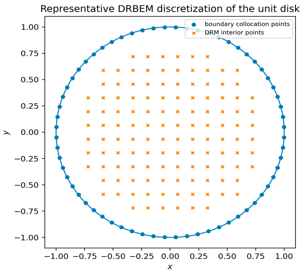
Figure 2.
Stiffness-induced failure of explicit fractional PECE integration and stable decay under the implicit Adams–Moulton correction.
Figure 2.
Stiffness-induced failure of explicit fractional PECE integration and stable decay under the implicit Adams–Moulton correction.
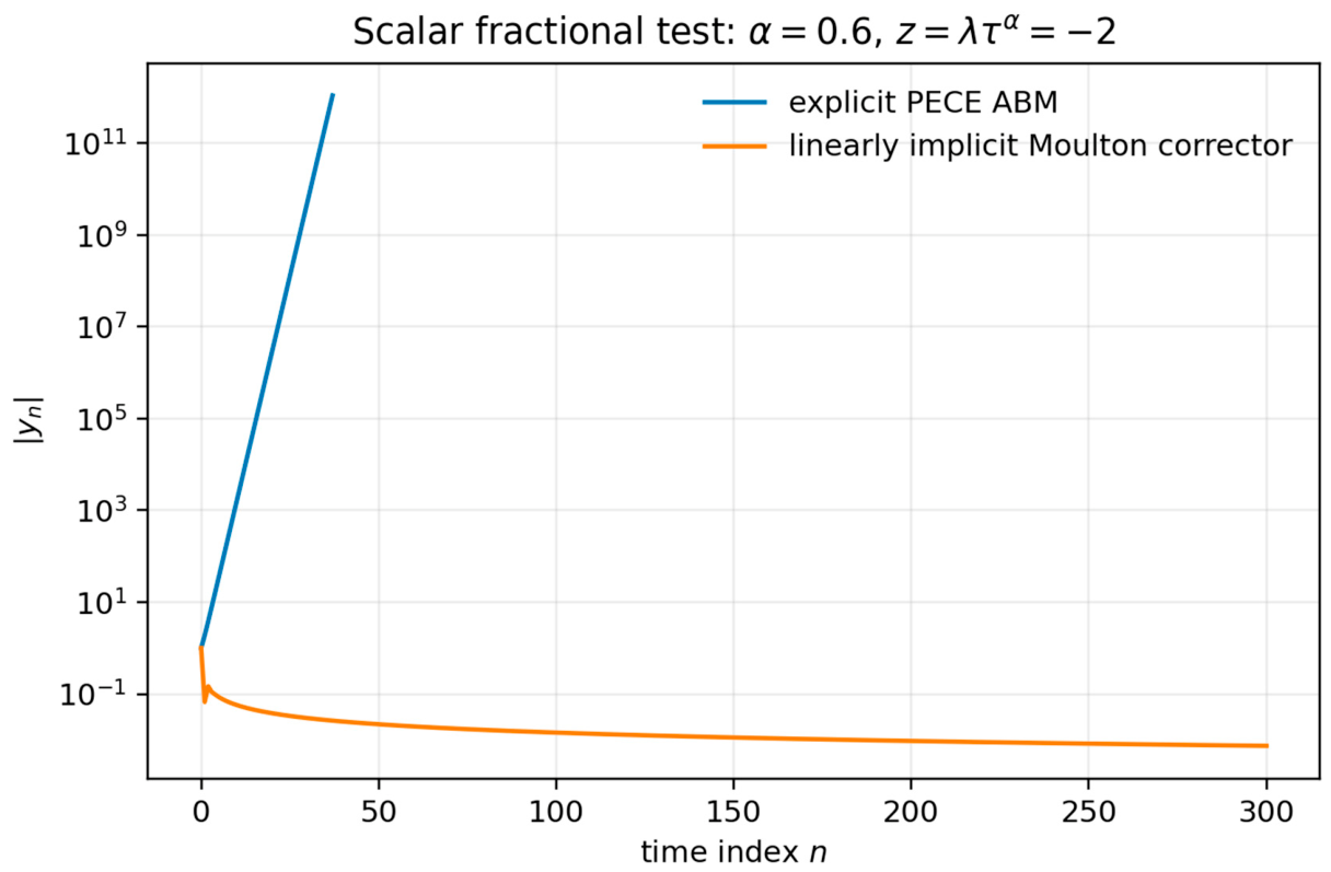
Figure 3.
Mesh-refinement evidence of near second-order DRBEM spatial convergence on the unit disk.
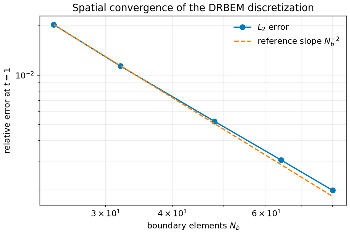
Figure 4.
Fractional-order-robust temporal convergence of the implicit Adams–Moulton correction for the manufactured benchmark.
Figure 4.
Fractional-order-robust temporal convergence of the implicit Adams–Moulton correction for the manufactured benchmark.
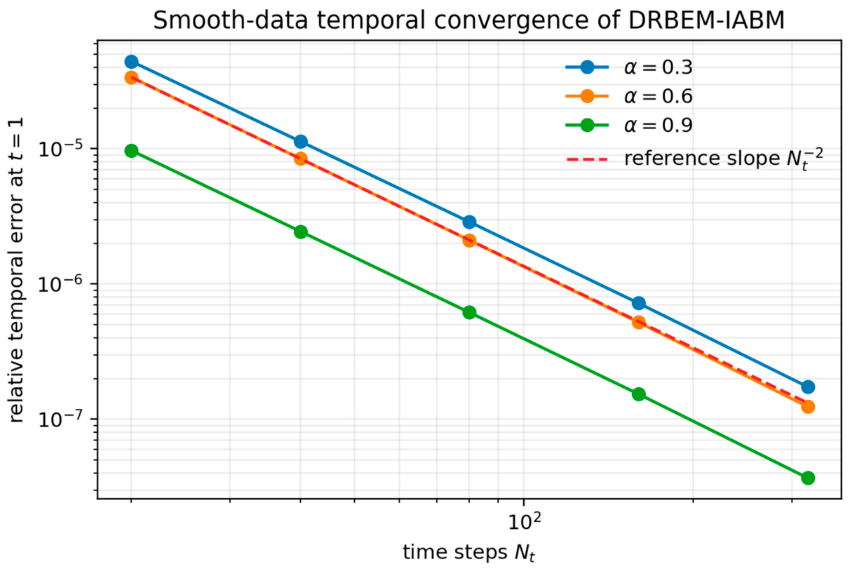
Figure 5.
Geometry-dependent spectrum of the nonconvex L-shaped DRBEM evolution operator.
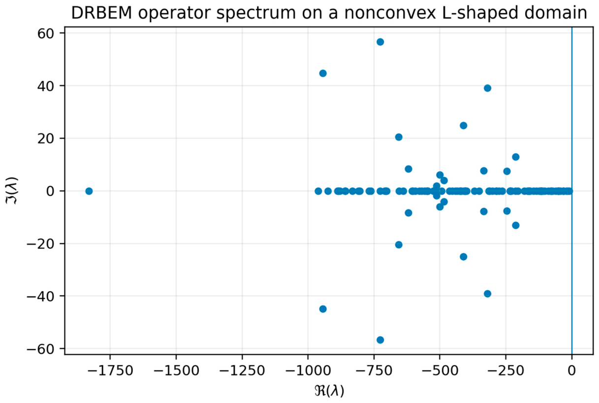
Figure 6.
Stable fractional diffusion field reconstructed by DRBEM-IABM on the nonconvex L-shaped domain.
Figure 6.
Stable fractional diffusion field reconstructed by DRBEM-IABM on the nonconvex L-shaped domain.
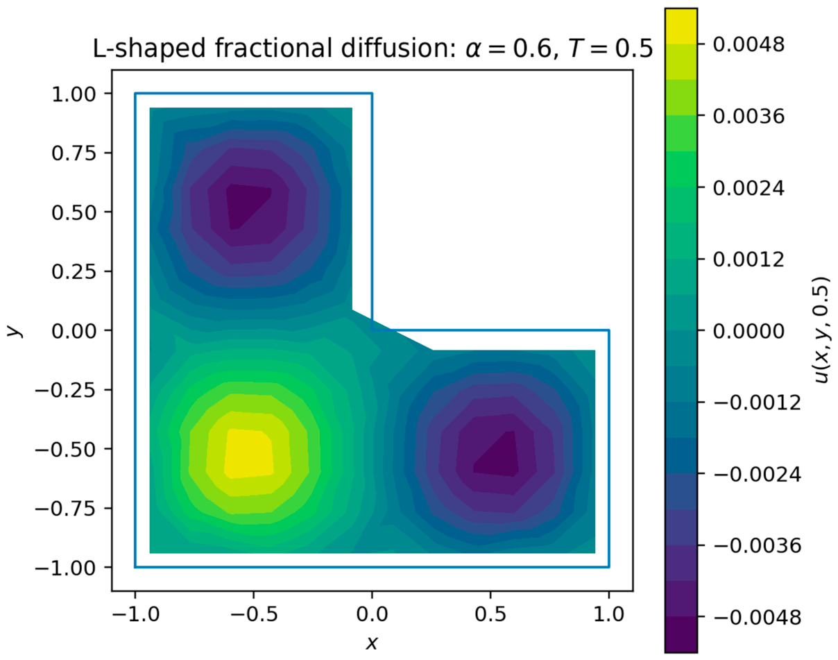
Figure 7.
Refinement-induced escalation of the explicit fractional PECE stability burden for the DRBEM disk operator.
Figure 7.
Refinement-induced escalation of the explicit fractional PECE stability burden for the DRBEM disk operator.
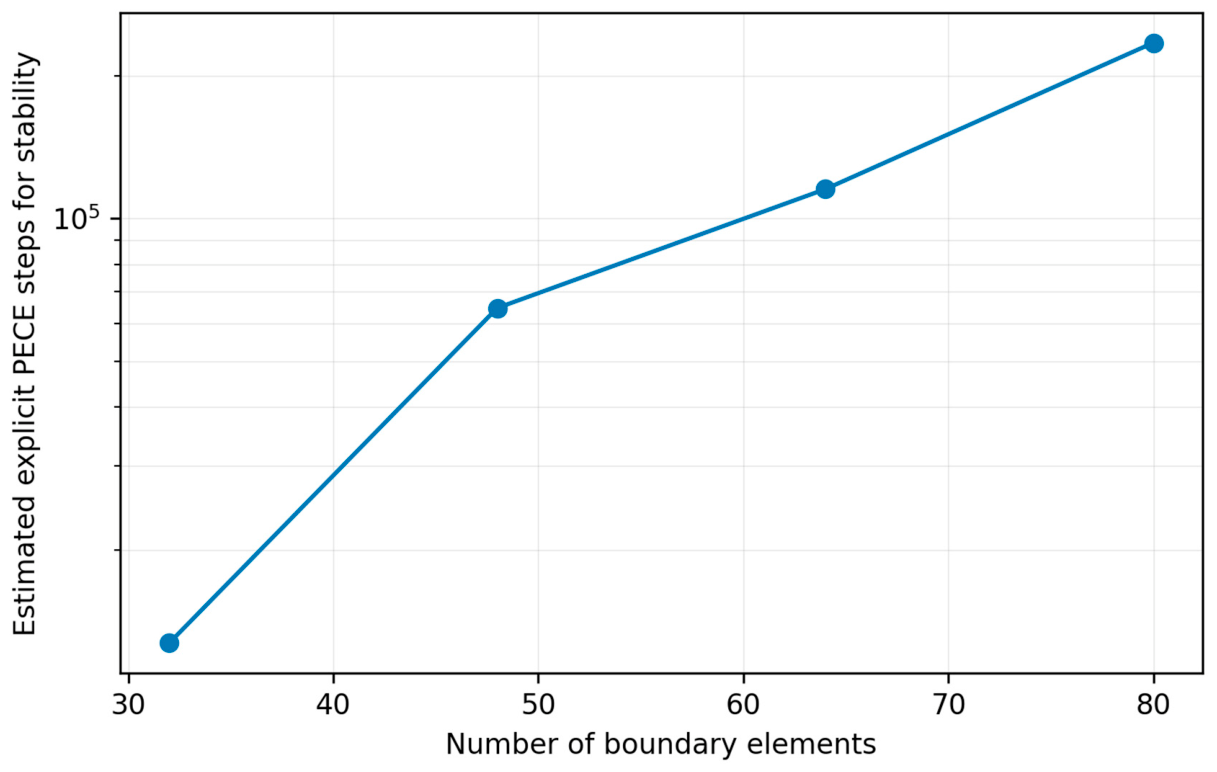

Table 1.
Negative-real-axis stability thresholds of the explicit fractional PECE scheme across representative fractional orders.
Table 1.
Negative-real-axis stability thresholds of the explicit fractional PECE scheme across representative fractional orders.
| 0.2 | 0.3 | 0.4 | 0.5 | 0.6 | 0.7 | 0.8 | 0.9 | 1.0 | |
|---|---|---|---|---|---|---|---|---|---|
| 1.1018 | 1.1667 | 1.2422 | 1.3293 | 1.4296 | 1.5447 | 1.6765 | 1.8274 | 2.0000 |
Table 2.
Spatial refinement and observed convergence of the DRBEM solution for the manufactured unit-disk problem.
Table 2.
Spatial refinement and observed convergence of the DRBEM solution for the manufactured unit-disk problem.
| Relative error | Observed order | error | ||
| 24 | 25 | – | ||
| 32 | 32 | 2.02 | ||
| 48 | 88 | 1.91 | ||
| 64 | 124 | 1.89 | ||
| 80 | 193 | 1.91 |
Table 3.
Time-step refinement of the implicit fractional Adams–Moulton correction for multiple fractional orders.
Table 3.
Time-step refinement of the implicit fractional Adams–Moulton correction for multiple fractional orders.
| Relative error | Observed order | ||
| 0.3 | 20 | – | |
| 40 | 1.97 | ||
| 80 | 1.98 | ||
| 160 | 2.00 | ||
| 320 | 2.05 | ||
| 0.6 | 20 | – | |
| 40 | 2.00 | ||
| 80 | 2.00 | ||
| 160 | 2.02 | ||
| 320 | 2.07 | ||
| 0.9 | 20 | – | |
| 40 | 1.99 | ||
| 80 | 1.99 | ||
| 160 | 2.00 | ||
| 320 | 2.06 |
The manufactured solution is intentionally smooth at the beginning, thus exhibiting the complete second-order temporal behavior for all three α's. This does not contradict the lower generic order associated with weak Caputo initial layers.
Table 4.
Refinement-driven growth of DRBEM spectral stiffness and the resulting explicit PECE time-step burden.
Table 4.
Refinement-driven growth of DRBEM spectral stiffness and the resulting explicit PECE time-step burden.
| Interior unknowns | Estimated explicit | Steps required for | ||
|---|---|---|---|---|
| 32 | 32 | 414.53 | 12,703 | |
| 48 | 88 | 1101.11 | 64,717 | |
| 64 | 124 | 1557.09 | 115,297 | |
| 80 | 193 | 2386.17 | 234,854 |
Table 5.
Temporal refinement on the nonconvex L-shaped domain under corner singularity and operator nonnormality.
Table 5.
Temporal refinement on the nonconvex L-shaped domain under corner singularity and operator nonnormality.
| Relative error | Observed order | ||
| 50 | – | ||
| 100 | 1.65 | ||
| 200 | 1.72 | ||
| 400 | 2.02 |
Table 6.
Methodological positioning of the proposed DRBEM-IABM framework relative to representative fractional and transient discretizations.
Table 6.
Methodological positioning of the proposed DRBEM-IABM framework relative to representative fractional and transient discretizations.
| Method | Spatial treatment | Time treatment | Geometry flexibility | Stability emphasis | Stiff diffusion treatment |
|---|---|---|---|---|---|
| Sohail et al. [1] | Global spectral collocation | Fractional ABM PECE | Best suited to simple spectral domains | Scalar and method-level stability analysis | Explicit predictor-corrector |
| Carrer et al. [9] | Direct Caputo boundary element formulation | Direct fractional-history treatment | General two-dimensional anisotropic media | Robustness and analytical verification | Formulation-dependent time marching |
| Khalighi et al. [11] | BEM with radial-basis source approximation | Chebyshev operational matrix | General two-dimensional geometries | Conditioning and convergence analysis | Global-in-time algebraic treatment |
| Yu et al. [28] | Isogeometric dual-reciprocity BEM | Precise integration for transient evolution | Exact NURBS geometry and heat-source problems | Accuracy and time-domain robustness | Implicit semidiscrete transient integration |
| DRBEM-IABM, present work | Dual-reciprocity BEM | Adams predictor with implicit fractional Moulton correction | Curved and nonconvex domains; extendable to three dimensions | Spectrum, numerical range, and resolvent certification | Stiff BEM diffusion operator treated implicitly |
Table 7.
Consolidated verification matrix linking numerical evidence to stability and convergence claims.
Table 7.
Consolidated verification matrix linking numerical evidence to stability and convergence claims.
| Verification target | Benchmark evidence | Observed behavior | Interpretation |
|---|---|---|---|
| Curved-domain spatial accuracy | Manufactured unit-disk refinement | Rates remain close to second order | Confirms DRBEM spatial consistency for smooth geometry and compatible forcing |
| Fractional temporal accuracy | Multiple-order time-step refinement | Rates approach second order for smooth compatible data | Confirms the high-order product-integration regime of the implicit correction |
| Stiffness robustness | Refined disk spectra and scalar stability test | Explicit step burden grows rapidly while implicit trajectories remain dissipative | Demonstrates removal of the dominant explicit diffusion restriction |
| Nonconvex geometry | L-shaped domain spectrum and field reconstruction | Stable left-half-plane spectrum with convergent time refinement | Supports geometry-aware stability on a re-entrant domain |
| Long-memory behavior | Continuation under several fractional orders | Smaller order retains a larger fraction of the initial-state norm | Recovers the expected slower anomalous diffusion response |
Disclaimer/Publisher’s Note: The statements, opinions and data contained in all publications are solely those of the individual author(s) and contributor(s) and not of MDPI and/or the editor(s). MDPI and/or the editor(s) disclaim responsibility for any injury to people or property resulting from any ideas, methods, instructions or products referred to in the content. |
© 2026 by the author. Licensee MDPI, Basel, Switzerland. This article is an open access article distributed under the terms and conditions of the Creative Commons Attribution (CC BY) license.
Copyright: This open access article is published under a Creative Commons CC BY 4.0 license, which permit the free download, distribution, and reuse, provided that the author and preprint are cited in any reuse.