

Submitted:
09 September 2026
Posted:
09 September 2026
You are already at the latest version
Abstract
Modin and Verdier observed favorable long-time energy behavior for nonholonomic leapfrog in a rotating constrained-spring example that their reversibility argument did not explain. We investigate a foundational question: which polynomial conservation laws follow from the reflected update independently of the driver? For planar rank-one constraints and 0 < h < 2, we prove that the modified quadratic energy generates all common polynomial invariants, except at h = \( \sqrt{2} \), where an independent quartic generator appears. At this step, a change of variables turns the update into an exchange of squared lengths. This mechanism extends to arbitrary orthogonal-projector sequences in any dimension. The classification identifies the conservation shared by the update family; the original passenger-energy observation remains a separate question.
Keywords:
nonholonomic leapfrog
; geometric numerical integration
; polynomial invariants
; modified energy
; invariant theory
1. Introduction
Leapfrog is a numerical method for approximating solutions of mechanical differential equations through staggered position and velocity updates. The nonholonomic version considered here, which also enforces a velocity constraint, was proposed by McLachlan and Perlmutter in 2006 [1] and revisited through a geometric construction by Ferraro, Iglesias, and Martín de Diego in 2008 [2]; later extensions and convergence results appeared in 2015 [3]. In 2020, Modin and Verdier [4] reported favorable leapfrog energy behavior in a perturbed continuously variable transmission (CVT) experiment that their reversibility argument did not explain. In 2023, Anahory Simoes et al. [5] revisited that model and observed favorable energy behavior for a Newmark composition method. These numerical observations motivate our study of the conservation laws built into the reflected leapfrog update.
1.1. The CVT Model and Its Energy Observation
The continuously variable transmission (CVT) model couples a spring subsystem, called the passenger, to a driver that changes its allowed velocity direction. With normalized masses and spring stiffnesses, passenger position and driver coordinate satisfy (Equation (12) [4])
Dots denote time derivatives. The potential V determines the independent driver motion; the constraint force enforces the allowed passenger velocity direction. With , the passenger energy is
the sum of kinetic and spring potential energies. The constraint force does no work because , so the continuous model conserves E. The numerical question is how well leapfrog retains this conservation. For the reconstruction below we use ; the caption records its distinction from the printed setup.
Modin and Verdier (Figure 6 [4]) compared numerical methods on this model. In the rotating, perturbed case, leapfrog maintained small errors in the energy of the spring subsystem over the reported interval with . Their reversibility argument did not explain this behavior, and they posed its explanation as an open problem (Section 6.1(2) [4]). Figure 1 shows our independent reconstruction of the qualitative contrast: leapfrog’s passenger-energy error stays small over the simulated interval while the midpoint discrete Lagrange–d’Alembert (DLA) error grows.
Anahory Simoes et al. (Section 5.2 [5]) later revisited the perturbed CVT and reported similarly favorable energy behavior for a Newmark composition method, alongside comparisons with leapfrog. Its explanation also remained open in that study. We analyze the reflected leapfrog update below; extending the classification to the Newmark composition would require a separate analysis.
Figure 2 summarizes the methods and numerical observations motivating our study.
1.2. From the Observation to a Classification Question
Figure 3 follows our investigation from the authors’ question to the estimate that remains open. Modin and Verdier ask what explains leapfrog’s favorable passenger-energy behavior in the rotating, perturbed CVT experiment (Section 6.1(2) [4]). Earlier reflection methods and convergence results provide the starting framework [1,2,3], but Modin and Verdier’s reversibility argument does not cover this case. These are the starting question and prior foundations in steps 1–2.
Our classification (step 3) isolates what the update conserves independently of the driver. The CVT velocity constraint in (1) has projector
We retain the reflected spring update and allow P to range over all planar rank-one orthogonal projectors, a larger family than the directions traced by this CVT driver. For planar rank-one projectors and , every common polynomial invariant is a polynomial in the modified quadratic energy , except at , where an additional generator appears. Special oscillator step sizes already occur in [1]; our contribution is completeness for the entire update family.
The energy identity (step 4) connects this classification to the original question. Writing for the correction in (19), conservation of gives , where is the correction along the numerical trajectory. At , no independent common polynomial supplies additional information beyond . Our next target (step 5) is therefore to use the actual CVT driver to bound the variation of over . The identity is established here; the small bound needed to explain the observation is not. Section 2, Section 3 and Section 4 develop the classification in step 3 of Figure 3; Section 5 establishes the energy identity in step 4 and states the remaining target in step 5.
Next, in Section 2, we write down how the method advances the spring and identify a quantity that remains unchanged after each step.
2. The Update and the Classification Problem
To begin proving the classification in step 3 of Figure 3, we specify the update family, identify its conserved quadratic energy, and state the full result in Theorem 1. We begin in Section 2.1 by writing down one step of the numerical method: how it calculates the next position and velocity when the allowed direction of motion can change.
2.1. The Reflected Spring Update
Let , where x is position and u is the incoming half-step velocity stored by the method. The stored velocity need not lie in the currently allowed direction. The spring stiffness and mass are normalized to one. For an orthogonal rank-one projector P, define by
The projector selects the allowed velocity direction. The map reflects across that direction. The synchronized velocity is , which satisfies the current constraint. We fix and allow a different P at every step.
With the update specified, Section 2.2 asks what stays unchanged as we repeat it. We first find an energy-like quantity that keeps the same value, even when the allowed direction changes, and then state which other conserved polynomials we aim to identify.
2.2. The Modified Energy and the Classification Question
We will use the quadratic quantities
The first is conserved for every projector; the second will identify the exceptional step. The proof below uses the norm-preserving reflection underlying [2]. We include the calculation for this spring update to make its arbitrary-projector scope explicit.
Proposition 1
(Modified energy). The update (2) preserves for every orthogonal projector P and every real h. Consequently remains constant along arbitrary projector sequences with fixed h.
Proof.
Write and . Then . Since is orthogonal,
Expanding and applying (4) gives zero at each step. □
We now ask whether any independent polynomial is conserved under the same freedom to change P.
Definition 1
(Common polynomial invariant). Fix . A polynomial is a common invariant if
for every and every rank-one orthogonal projector P. We denote the algebra of these polynomials by .
Theorem 1
(Complete classification). For the family (2) with and ,
At , the generators and are algebraically independent.
In other words, every common polynomial invariant is a polynomial in the displayed generators, with no restriction on degree. At the exceptional step, the additional generator has degree four; the space of homogeneous quadratic invariants is still one-dimensional. Next, in Section 3, we show where the extra quartic comes from: at , the update exchanges two squared lengths, producing another conserved quantity.
3. Finding the Exceptional Generator
The modified energy supplies one polynomial generator. We now construct the additional quartic at by changing coordinates; completeness will require a separate argument.
Quartic integrals already occur in discrete nonholonomic mechanics: Fedorov and Zenkov (Theorem 6.2 [6]) give an integral quartic in quaternion variables for the discrete Suslov system. Here the question is conservation under every projector choice and the completeness of the resulting algebra. The extra generator comes from an exchange of lengths.
3.1. A Change of Variables Exchanges Lengths
Introduce
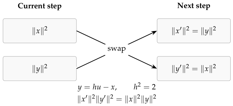
At the first term vanishes. The remaining reflection preserves the length of y, while the sign change preserves the length of x. Therefore
The squared lengths exchange values. Their sum and product remain unchanged, as illustrated in Figure 4.
3.2. The Quartic Invariant
The length exchange yields an exact conservation law, even beyond the planar setting of our classification.
Proposition 2
(Resonant conservation in any dimension). Let belong to a real inner-product space, let , and use (2) with any orthogonal projector P. Then
Consequently and are conserved along every sequence of such updates, with fixed h.
Proof.
The difference changes sign under the exchange, and the product is unchanged. In particular, . □
For example, take a unit vector e. The states and both have , whereas equals 0 and 1, respectively. The quartic therefore distinguishes states that the quadratic energy does not. Next, in Section 4, we show that these quantities account for every common polynomial invariant. We do this by studying the transformations built from repeated updates and what those transformations leave unchanged.
4. Proving that the Generators Are Complete
Finding conserved quantities gives only part of the classification. We now show that every common polynomial invariant belongs to the algebra generated by them. First we identify the group generated by the updates; then we determine its invariant polynomials.
4.1. Identifying the Group Generated by the Updates
A common invariant must survive every composition of the updates. The group generated by all constraint directions therefore determines what an invariant can distinguish. We work in the coordinates and write
Here is the update for , and rotates position and velocity together. Every rank-one orthogonal projector therefore gives an update . Direct multiplication gives
The eigenvalues of are , each twice. Thus is positive definite on the interval under consideration.
Let be the closed group generated by the projector updates. For , the group is a closed subgroup of . In these coordinates, becomes ordinary squared length. Here denotes all length-preserving linear maps in four dimensions, and its determinant-one subgroup. The notation describes two independent plane rotations; is the cyclic group of order four. At resonance their semidirect product records how an order-four update rearranges those rotations.
Theorem 2.
For ,
If , the group is isomorphic to . Its identity component independently rotates two orthogonal planes, and a generator of exchanges those planes.
Proof. Step 1: Recover simultaneous rotations. We first show that contains all simultaneous rotations . In this proof write , , and
The curve lies in and starts at the identity. Its derivative is , so belongs to the Lie algebra of . Conjugating by A puts every in that Lie algebra. The matrices in (10) satisfy
Since , this puts Z in the Lie algebra. Consequently
Step 2: Generate the group away from resonance. Suppose first that . Here we seek matrix generators for the Lie algebra, rather than generators of conserved polynomials. The Lie algebra contains the six matrices
For each matrix, retain its entries in positions , in that order, and form the six-column matrix using (14). Its determinant is
Equations (12) and (15) are finite matrix identities; (10) and the specified entries give all data needed to check them. The six matrices are independent and G-skew, so they span the six-dimensional Lie algebra . After conjugation by , the identity component is therefore . Since , the full group is .
Step 3: Identify the exceptional group. Now suppose , and put . Direct multiplication gives
The matrix
is a G-self-adjoint involution. Its eigenspaces and have dimension two and are G-orthogonal. On , ; on , . Hence the subgroup
independently rotates these planes and is a two-dimensional torus. Conjugation by A maps to , so it normalizes . No element , , lies in : its conjugation sends Z to , respectively, whereas all elements of commute with Z. Thus is a compact group isomorphic to . By (13) it is exactly . Finally, , so A exchanges and . Conjugation by makes these planes Euclidean-orthogonal. □
4.2. Recovering All Invariant Polynomials
The group description now completes the classification: away from resonance, only the total squared length matters; at resonance, the two plane lengths supply the additional generator.
Proof
(Proof of Theorem 1). A polynomial preserved by each invertible update is also preserved by its inverse, by every finite product, and by the closure of those products. Thus the common polynomial invariants are precisely the -invariant polynomials.
If , Theorem 2 reduces the question to . An invariant polynomial is constant on every sphere. Its restriction to a coordinate axis is an even polynomial, say ; invariance then gives everywhere. This proves that the invariant algebra is .
At , let and be the squared -lengths of the components in the two planes from (17):
The last equality follows from . In the reflection coordinates , these are simply and . Independent rotations on the two planes force every invariant polynomial to belong to . Indeed, in complex coordinates on each plane, rotation invariance forces each monomial to contain equal powers of the coordinate and its conjugate. The generator exchanges the two radii. The full invariant algebra is therefore the algebra of symmetric polynomials in them:
There is no polynomial relation between these two generators. The radii range independently over the nonnegative quadrant, and the map has nonzero Jacobian when . Its image therefore contains an open set, on which no nonzero polynomial can vanish. This completes the classification. □
Next, in Section 5, we relate these conserved quantities to the spring subsystem’s physical energy and identify the estimate still needed to explain the observed behavior at .
5. From Modified Energy to the Remaining CVT Estimate
The common polynomial classification is now complete. Steps 4–5 of Figure 3 concern a different task: connecting that conservation to physical energy and identifying the estimate needed for the observed CVT behavior.
5.1. The Physical-Energy Identity
To relate the conserved quantity to physical energy, define the synchronized velocity and the remaining numerical component . Orthogonality gives
Thus conservation of does not by itself imply conservation of physical energy. The energy-error estimate depends on the variation of the combined correction. The additional invariant at is an exact property of a particular step size, not a small-step accuracy result.
5.2. Future Work: The CVT Estimate at
At step n, use the projector at position and define
Here is the synchronized passenger velocity; remains the stored half-step velocity. Equation (19) and conservation of give . Our proposed target for the reported experiment is a small quantitative bound on
using the actual CVT driver and initial data. This estimate is not proved here. It concerns the variation of the combined correction; neither term must vanish separately. An estimate uniform over all n would establish the stronger all-time result.
The next step is to use the ordered projector sequence generated by the numerical CVT driver to estimate . One route is a direct bound that accounts for cancellation between steps. Another is to seek a conserved or nearly conserved quantity depending on the driver’s phase as well as on , and quantify its relation to . Theorem 1 does not exclude such driver-dependent quantities. Either route must produce a bound small enough to account for the observed energy error, rather than merely show that the trajectory stays bounded.
6. Conclusions
We have answered which polynomial conservation laws are shared by every planar rank-one projector update of nonholonomic leapfrog. For fixed , the modified energy generates all common polynomial invariants, except at , where the additional generator appears. The length-exchange argument explains this exceptional invariant, and the group analysis proves that the generators are complete.
At , the classification shows that no independent common polynomial invariant adds information beyond . We also established the exact identity , connecting modified-energy conservation to physical-energy error. These results identify both the conservation supplied by the update and the correction whose variation controls the error.
The original CVT energy observation remains open. Section 5.2 identifies the driver-dependent estimate needed to explain it at .
Funding
This research received no external funding.
Institutional Review Board Statement
In this section, you should add the Institutional Review Board Statement and approval number, if relevant to your study. You might choose to exclude this statement if the study did not require ethical approval. Please note that the Editorial Office might ask you for further information. Please add “The study was conducted in accordance with the Declaration of Helsinki, and approved by the Institutional Review Board (or Ethics Committee) of NAME OF INSTITUTE (protocol code XXX and date of approval).” for studies involving humans. OR “The animal study protocol was approved by the Institutional Review Board (or Ethics Committee) of NAME OF INSTITUTE (protocol code XXX and date of approval).” for studies involving animals. OR “Ethical review and approval were waived for this study due to REASON (please provide a detailed justification).” OR “Not applicable” for studies not involving humans or animals.
Informed Consent Statement
Any research article describing a study involving humans should contain this statement. Please add “Informed consent was obtained from all subjects involved in the study.” OR “Patient consent was waived due to REASON (please provide a detailed justification).” OR “Not applicable” for studies not involving humans. You might also choose to exclude this statement if the study did not involve humans.
Data Availability Statement
The supplementary archive contains the reconstructed trajectories and plotted data for Figure 1, numerical and symbolic source code, and selected Lean proofs. These data are an independent reconstruction, not the original authors’ data.
Acknowledgments
OpenAI ChatGPT/Codex agents assisted with literature searches, mathematical exploration and proof development, programming, manuscript drafting and editing, and internal review. AI assistance does not constitute independent peer review or certification of novelty; the author is responsible for the final content.
Conflicts of Interest
The author declares no conflicts of interest.
References
- McLachlan, R. I.; Perlmutter, M. Integrators for nonholonomic mechanical systems. J. Nonlinear Sci. 2006, 16, 283–328. [Google Scholar] [CrossRef]
- Ferraro, S.; Iglesias, D.; Martín de Diego, D. Momentum and energy preserving integrators for nonholonomic dynamics. Nonlinearity 2008, 21(8), 1911–1928. [Google Scholar] [CrossRef]
- Ferraro, S.; Jiménez, F.; Martín de Diego, D. New developments on the geometric nonholonomic integrator. Nonlinearity 2015, 28(4), 871–900. [Google Scholar] [CrossRef]
- Modin, K.; Verdier, O. What makes nonholonomic integrators work? Numer. Math. 2020, 145, 405–435. [Google Scholar] [CrossRef]
- Simoes, A. Anahory; Ferraro, S. J.; Marrero, J. C.; de Diego, D. Martín. A nonholonomic Newmark method. J. Comput. Appl. Math. 2023, 421, 114873. [Google Scholar] [CrossRef]
- Fedorov, Y. N.; Zenkov, D. V. Discrete nonholonomic LL systems on Lie groups. Nonlinearity 2005, 18(5), 2211–2241. [Google Scholar] [CrossRef]
Figure 1.
Reconstructed passenger-energy comparison inspired by (Fig. 6 [4]); these are not the authors’ original data. Here , , , and . We plot a 30-time-unit running mean of , with . The potential and perturbation follow our reconstruction of the figure because the source’s printed setup is inconsistent. This finite experiment does not establish an all-time bound.
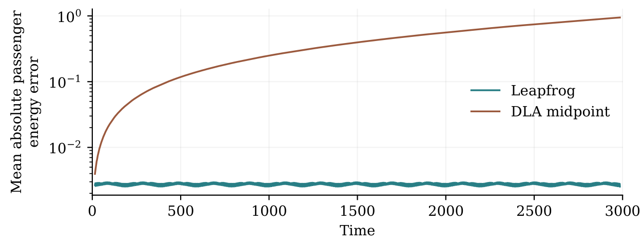
Figure 2.
Earlier methods and CVT experiments. The timeline distinguishes the geometric foundations from the later numerical observations. Earlier quartic integrals for a different system [6] are discussed in Section 3.

Figure 3.
Roadmap from the authors’ question to the remaining estimate. Arrows show the research sequence, not implications between cited results. The dashed final step remains open.
Figure 3.
Roadmap from the authors’ question to the remaining estimate. Arrows show the research sequence, not implications between cited results. The dashed final step remains open.
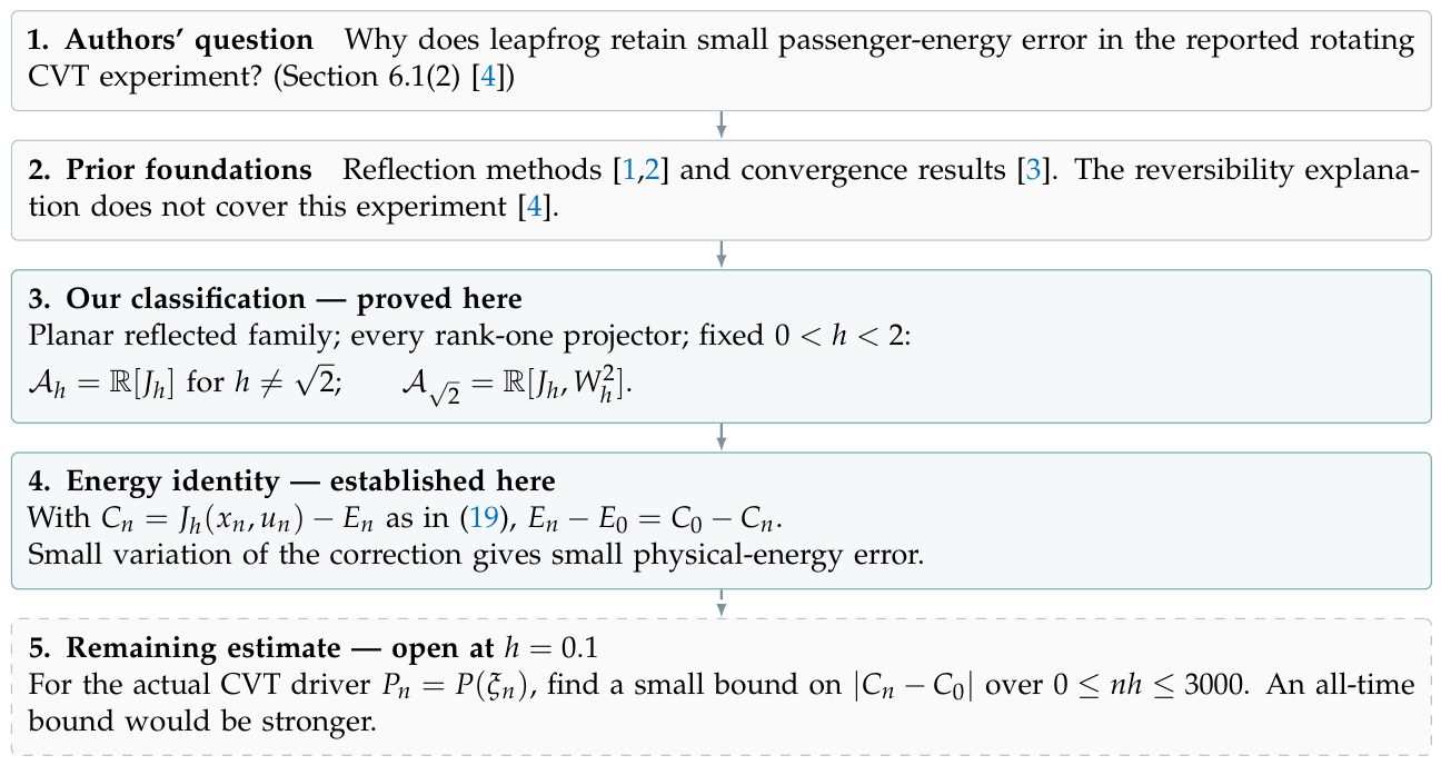
Figure 4.
At , one step exchanges the squared lengths of x and . The reflection may change at the next step; the sum and product of the squared lengths remain conserved.
Figure 4.
At , one step exchanges the squared lengths of x and . The reflection may change at the next step; the sum and product of the squared lengths remain conserved.
Disclaimer/Publisher’s Note: The statements, opinions and data contained in all publications are solely those of the individual author(s) and contributor(s) and not of MDPI and/or the editor(s). MDPI and/or the editor(s) disclaim responsibility for any injury to people or property resulting from any ideas, methods, instructions or products referred to in the content. |
© 2026 by the authors. Licensee MDPI, Basel, Switzerland. This article is an open access article distributed under the terms and conditions of the Creative Commons Attribution (CC BY) license (http://creativecommons.org/licenses/by/4.0/).
Copyright: This open access article is published under a Creative Commons CC BY 4.0 license, which permit the free download, distribution, and reuse, provided that the author and preprint are cited in any reuse.