

Submitted:
08 September 2026
Posted:
09 September 2026
You are already at the latest version
Abstract
We present a theoretical and numerical study of the Self-Consistent Spectral Potential Mean-Field (SC-SPMF) method for the description of structure and stability of phase transitions in condensed matter. The method extends the original Spectral Potential Mean-Field (SPMF) approach by introducing a fully self-consistent cycle between the Kirkwood relation and the Fisher equation. The SC-SPMF method determines the coordination shell in condensed matter, providing a genuinely predictive framework for the study without requiring approximate functionals or closure relations.
The method is applied to the solid-to-liquid and liquid-to-solid phase transitions of argon, a prototypical monatomic system with well-characterized experimental and simulation data. The temperature evolution of key parameters of radial distribution function and potential of mean force clearly identifies the phase transition at approximately 86 K, in agreement with the experimental melting temperature of argon (83.8 K).
A central result is the formulation of a spectral criterion for stability: the transition is marked by a change in the curvature of the first eigenvalue of the Fischer equation μ1(T), specifically by the temperature at which the second derivative d2μ1/dT2 becomes positive. This criterion does not rely on the absolute value of μ1, but on a qualitative change in the spectral response of the system, providing a system-independent fingerprint of the onset of the liquid phase.
The method captures hysteresis and metastability between heating and cooling paths, with a hysteresis width of approximately 1.6 K, consistent with the first-order nature of the transition. The critical exponent β is found to differ between the two paths: β≈0.36 for the heating (close to the 3D Ising model value of 0.326) and β≈0.51 for the cooling (close to the mean-field value of 0.5). This difference reflects the role of short-range or long-range interactions in determining the effective critical behavior along melting or crystallization paths, respectively. This spectral interpretation offers a new perspective on phase stability, hysteresis, and critical phenomena, making the SC-SPMF method a powerful and original tool for the study of condensed matter.
Keywords:
potential of mean force
; radial distribution function
; Fisher equation
; Kirkwood relation
; first-order phase transition
; critical exponent
; hysteresis
; metastability
; coordination shells
; liquid-solid transition
; argon
1. Introduction
The theoretical description of phase transitions in condensed matter has been a central challenge in statistical thermodynamics for over a century. From the early phenomenological theories of van der Waals and Landau to the modern renormalization group approach of Wilson, the study of phase transitions has driven the development of many of the most powerful concepts in chemical-physics. Despite these advances, the prediction of phase transition temperatures, the characterization of critical behavior, and the understanding of metastability and hysteresis remain active areas of research.
The solid-to-liquid and liquid-to-solid phase transitions are one of the most fundamental and ubiquitous phenomena in nature. It governs the formation of crystals from melts, the structure and stability of glaciers, the behavior of magma, the processing of polymers in industry. Yet, despite its importance, a theoretical description of melting and crystallization remains elusive. The transitions are strongly first-order, characterized by a discontinuity in density and entropy, and is accompanied by metastable states (superheating and supercooling) and hysteresis. These features make it challenging to study theoretically, as they require a description of both stable and metastable phases, as well as the kinetics of nucleation and growth.
The theoretical study of phase transitions has evolved through several stages: phenomenological theories; Statistical thermodynamics of fluids; Density Functional Theory; Renormalization Group approach; Computer simulations.
The van der Waals equation of state (1873) provided the first phenomenological theory of the liquid-gas transition, capturing the coexistence curve and the critical point. Landau’s theory of phase transitions (1937) introduced the concept of an order parameter and provided a general framework for describing second-order transitions [1,2,3,4,5].
The development of integral equation theories, such as the Ornstein-Zernike (OZ) equation (1914) and its closures (Percus-Yevick, 1958; Hypernetted-Chain, 1960), provided the statistical thermodynamics of fluid structure. These theories relate the radial distribution function g(r) to the interparticle potential u(r) through a set of integral equations [6,7,8,9].
Classical Density Functional Theory (cDFT), developed by Evans and others in the 1970s and 1980s, provides a formally exact framework for studying solids and fluids. The theory expresses the grand potential (at fixed temperature, volume, and chemical potential ) as a functional of the density profile ρ(r), and the equilibrium density is obtained by minimization [10,11,12,13,14,15,16].
Wilson’s renormalization group (RG) theory (1971) provided a rigorous explanation of critical phenomena, showing that the singular behavior near critical points is due to the divergence of the correlation length [17,18,19,20,21,22,23,24,25].
Molecular dynamics (MD) and Monte Carlo (MC) simulations have provided invaluable insights into phase transitions, allowing the direct calculation of structural and thermodynamic properties from first principles [26,27,28,29,30,31,32].
Despite the remarkable successes of the theoretical methods, each approach has inherent limitations that restrict its applicability, accuracy or predictive power. cDFT requires approximate excess free energy functionals, which introduce systematic errors. The choice of functional is often system-dependent and can significantly affect the results. OZ integral equation theory requires closure relations that introduce thermodynamic inconsistencies and are not exact for three-dimensional systems. Renormalization group is a powerful theoretical tool but is challenging to apply to specific systems, especially those with complex interactions. Computer simulations are computationally expensive and provide results that are statistical in nature, requiring careful analysis of finite-size effects and sampling errors. These limitations and difficulties have motivated the development of new theoretical approaches, such as the Self-Consistent Spectral Potential Mean-Field (SC-SPMF) method.
2. The Self-Consistent SPMF (SC-SPMF) Method
In our previous work, we introduced the Spectral Potential Mean-Field (SPMF) method as an alternative to cDFT and OZ theory [33]. The SPMF method provides a spectral interpretation of the coordination shell structure in condensed matter: the Potential of Mean Force (PMF) is modeled as a weighted sum of Lennard-Jones (LJ-PMF) potentials, validated against the Kirkwood PMF derived from a known radial distribution function g(r). This LJ-PMF is then introduced into the Fisher equation for the correlation amplitudes.
The SPMF method demonstrated that, with a physically motivated choice of the PMF parameters, the essential structural features of liquid argon, Face-Centered Cubic (FCC) and Hexagonal Close-Packed (HCP) lattices could be reproduced. However, the method was not self-consistent: the input g(r) was not modified by the spectral analysis, and the comparison between the reconstructed and the original g(r) served only as a validation test.
In this work, we extend the SPMF method to a fully self-consistent scheme—the Self-Consistent SPMF (SC-SPMF) method—in which the coordination shell positions are not assumed a priori but emerge iteratively from the calculation itself. The self-consistency is achieved by iterating between the Kirkwood relation and the Fisher equation until the PMF and the radial distribution function are mutually consistent.
The SC-SPMF method represents a significant advancement over the original SPMF approach: the structure is determined self-consistently, without requiring experimental input (1); the eigenvalue spectrum provides a direct measure of the stability of the coordination shells (2); the method can be applied to study phase transitions by following the temperature evolution of the spectral parameters (3).
3. Why Argon?
The choice of argon as a test system is motivated by the wealth of well-characterized experimental and computational data available, which provides a rigorous benchmark for validating the SC-SPMF method. The structural characterization of liquid argon is anchored by the classic neutron diffraction study of Yarnell, Katz, Wenzel, and Koenig (1973), which provides the standard reference for the radial distribution function g(r) and structure factor S(q) at 85 K. This dataset has become the benchmark for validating theoretical models and simulation methods, as it captures the detailed structure of the liquid with high precision [34].
The phase diagram of argon in the low-temperature region has been extensively characterized through a combination of experimental measurements and computational studies. This temperature range is particularly relevant for the study of the liquid-solid transition, as it encompasses the melting temperature of argon at ambient pressure and the surrounding metastable regions where superheating and supercooling phenomena occur. The melting curve of argon at low pressures has been accurately determined using various experimental techniques. At ambient pressure, the melting temperature of argon is well established at 83.8 K . This value serves as a fundamental reference point for validating theoretical models and simulation methods. The solid phase of argon at these temperatures adopts the FCC structure, with a lattice parameter that varies with temperature due to thermal expansion. The liquid phase, on the other hand, exhibits a structure characterized by broad and damped oscillations in the radial distribution function, reflecting the thermal motion and structural disorder of the atoms [35,36].
Below the melting temperature, the liquid can be supercooled, remaining in a metastable liquid state down to temperatures significantly below the equilibrium melting point. Above the melting temperature, the solid can be superheated, persisting in a metastable solid state. These metastable states are of particular interest because they are directly accessible to the SC-SPMF method, which captures the hysteresis between heating and cooling paths.
Monte Carlo methods have been useful in validating interatomic potentials. Barker, Fisher, and Watts (1973) used the pair potential of Barker with the Axilrod-Teller three-body interaction, obtaining excellent agreement with experimental pressure and internal energy data for both solid and liquid argon. These calculations demonstrated the importance of including three-body interactions for achieving quantitative agreement at high densities. Barker (1987) further extended these calculations to high pressures up to 800 kbar, achieving good agreement with experimental data [37,38].
MD simulations have provided deep insights into argon’s phase behavior. Mahnama et al. studied the transition from solid to supercritical state induced by shock waves in argon atoms arranged in a FCC structure. Recent MD work by Ran and Bertola (2024) investigated the isochoric transition to the supercritical state, using a Lennard-Jones interatomic potential and analyzing the evolution of the system during phase transitions. Studies by Kim and Ha examined the transition to the supercritical state in argon layers confined between platinum plates. Investigations of nanoconfined argon have also revealed solid-liquid-solid phase transitions and hysteresis in force-distance profiles [39,40,41,42]. Beyond simulations, analytical group-theoretical studies by Góźdź (2001) have provided rigorous criteria for identifying spontaneous solidification in argon, proving that the order parameter symmetries of the liquid-solid transition appear in the two-body density. This provides a formal foundation for understanding the symmetry-breaking associated with crystallization [43,44,45,46,47,48,49].
In conclusion, argon is an ideal test case for several reasons: argon atoms interact through a spherically symmetric Lennard-Jones potential, which is well-understood and accurately represents the interatomic forces (1); the radial distribution function of liquid argon has been measured with high precision by neutron diffraction (Yarnell et al., 1973), providing reliable reference data (2); the melting temperature of argon at ambient pressure (83.8 K) is well known, as are its thermodynamic properties (3); argon is computationally inexpensive to simulate, making it an ideal test case for new methods.
4. From SPMF to SC-SPMF Method
The Potential of Mean Force (PMF) is one of the most fundamental concepts in the statistical thermodynamics of liquids and solids. Introduced by Kirkwood in his seminal 1935 paper of fluid mixtures, the PMF represents the effective potential between two particles in a medium, averaged over all configurations of the remaining particles.
The PMF is defined through the Kirkwood relation:
where, g(r) is the radial distribution function, which gives the probability of finding a particle at a distance r from a reference particle, relative to the ideal gas value; k is the Boltzmann constant; T is the absolute temperature. C is a constant fixed by the condition UK(∞)=0, which ensures that the PMF vanishes at infinite separation.
The radial distribution function g(r) is defined as:
where, ρ(r) is the local density of particles at a distance r from a reference particle; is the average density of the system (number of particles per unit volume).
In the case of an ideal gas, the particles are completely uncorrelated, and the local density around a reference particle is constant and equal to the average density: ρ(r)=ρ0. Thus, for an ideal gas, we have g(r)=1 for every r. This normalization condition for g(r) simplifies the Kirkwood equation. Since UK(∞)=0 and g(∞)=1, the additive constant vanishes, yielding C=0.
This means that g(r) measures the deviation of the structure of the real system from that of an ideal gas: in an ideal gas, there is no correlation between the positions of the particles, so the probability of finding a particle at a distance r from another is independent of r. The PMF has a clear physical interpretation: it represents the reversible work required to bring two particles from infinite separation to a distance r, averaged over all configurations of the remaining particles: this work includes both the direct interaction between the two particles and the indirect interactions mediated by the surrounding medium.
The Kirkwood equation for the PMF can be written as:
where ⟨F(r)⟩ is the average force between two particles at distance r. This equation shows that the PMF is the potential whose gradient gives the mean force.
−∇UB(r)=⟨F(r)⟩
The Fisher equation, introduced by Fisher in 1964 in the context of correlation functions near the critical region of simple fluids, is a fundamental equation in the theory of phase transitions and critical phenomena. In its original form, the Fisher equation describes the behavior of the correlation function near the critical point, where the correlation length diverges.
In our context, the Fisher equation takes the form of a Schrödinger-like eigenvalue equation for the correlation amplitudes ψi(r):
This analogy is not merely formal and it has deep physical implications: the potential UK(r) is the PMF, which is the effective potential between two particles; the eigenfunctions ψi(r) are the correlation amplitudes, which describe the spatial structure of the correlations; the eigenvalues μi are the energy levels of the correlation modes.
The eigenvalues and eigenfunctions of the Fisher equation have a clear physical interpretation: these are the potential levels associated with the coordination shells. Negative eigenvalues correspond to bound states (stable coordination shells), while positive eigenvalues correspond to unbound states (delocalized correlations). Eigenfunctions ψi(r) are the correlation amplitudes: the square of the eigenfunction, ∣ψi(r)∣2, gives the probability density of finding a particle in the i-th correlation mode. The linear combination of squared eigenfunctions is the standard form in statistical mechanics for reconstructing g(r) from the eigenfunctions, in analogy with the electron density in quantum DFT [50,51,52].
The stability of the system is encoded in the eigenvalue spectrum of the Fisher equation. Negative eigenvalues (μi<0) indicate bound states, corresponding to localized coordination shells and a stable solid phase. As the temperature increases, the eigenvalues become less negative; when the first eigenvalue μ1 reaches zero, the last bound state vanishes, and the system undergoes a transition to a delocalized liquid phase: the condition μ1=0 would thus provide a spectral criterion for the phase transition. However, as we shall see, the actual behavior of μ1(T) reveals a more nuanced picture. In our SC-SPMF simulations for argon, μ1 does not vanish at the transition, but remains negative even in the liquid phase, reflecting the persistence of short-range order: the transition is marked by the crossing of a characteristic threshold value and, more significantly, by a change in the curvature of μ1(T).
In the equations of the SC-SPMF method, thermodynamics enters exclusively through the temperature T and the density ρ. The density is implicitly contained in the radial distribution function g(r), since g(r)→1 as r→∞, recovering the ideal-gas limit.
The SC-SPMF method is formulated within the canonical ensemble (N,V,T fixed). In this ensemble, the pressure is not an independent variable; rather, it is a derived thermodynamic property that is obtained after the structure of the system—i.e., the radial distribution function g(r)—has been determined. The transition temperatures calculated with the SC-SPMF method— Tm≈86.3 K for the heating path and Tm≈87.9 K for the cooling path—are referred to the density corresponding to ambient pressure. This density is fixed by the input data: for the solid phase, it is determined by the lattice parameter a=5.26 Å; for the liquid phase, it is determined by the experimental g(r) of Yarnell et al. [34]. Thus, while the pressure is not an input parameter, it is implicitly set by the choice of the structural input data, ensuring that the calculated transition temperatures correspond to the experimentally relevant thermodynamic conditions.
The SC-SPMF method proceeds through the following iterative steps:
Step 1: Initialization
Start with an initial . This can be obtained from: experimental data (e.g., neutron diffraction for liquid argon) ; a theoretical model (e.g., the ideal FCC lattice for solid argon); a simple approximation (e.g., the Percus-Yevick solution for hard spheres).
Step 2: Kirkwood step
At each iteration n, the PMF is updated using the current radial distribution function:
Step 3: Parametrization of the PMF
Represent the PMF as a weighted sum of Lennard-Jones terms:
where: rm is the position of the minimum of the well (coordination distance of shell m); ϵm is the depth of the well (kcal/mol); σm is the width of the well (Å); Sm(r) is a sigmoid function that modulates the contribution of each term [33].
The parameters can be updated by: fitting, minimizing the squared difference between and , or setting rm to the position of the m-th peak of g(r), ϵm to the depth of the well, and σm to the width of the peak. In this work, we use the physical assignment approach, which ensures that the parameters retain a clear physical meaning and that the method does not become computer-time expensive.
Step 4: Fisher step
Solve the Fisher equation with :
This equation is solved numerically on a grid in r. The boundary conditions are ψi(0)=0 and ψi(∞)=0.
Step 5: Reconstruction of g(r)
Reconstruct as a linear combination of the squared eigenfunctions of Fischer equation:
The coefficients are statistical weights, chosen to ensure that for . In our implementation, , where are the eigenvalues of Fischer equation.
Step 6: Kirkwood update
Compute a new PMF from the reconstructed :
Step 7: Convergence check
Check if the changes in the coordination shell positions rm:
If the criterion is satisfied, stop; otherwise, return to Step 3.
The SC-SPMF cycle is designed to converge to a fixed point where the PMF and the g(r) are mutually consistent. The convergence is typically fast (6–10 iterations) because the cycle is well-posed and the equations are smooth.
The convergence tolerance is chosen to ensure numerical accuracy: typical value isÅ. The weighted Lennard-Jones parametrization of the PMF is a key element of the SC-SPMF method. It provides a compact, physically motivated representation of the PMF that is smooth, stable, and interpretable. The LJ representation has several advantages: the LJ potential is the standard model for intermolecular interactions in noble gases (1); the parameters rm, ϵm, σm have clear physical meanings (2); the LJ potential is smooth and differentiable, which is essential for the numerical solution of the Fisher equation (3); the LJ potential is stable and well-behaved, unlike the Kirkwood PMF, which can be noisy (4).
5. The Spectral Interpretation of Phase Transitions
The Fisher operator is a Hermitian operator with a discrete spectrum of eigenvalues μi. The spectrum can be divided into two regions: bound states, μi<0 corresponding to localized correlation modes (coordination shells); continuum states, μi→0 corresponding to delocalized correlations.
The phase transition is interpreted as a spectral transition of the Fisher operator. The system is stable when the PMF is deep enough to support bound states, and unstable when it is not. The first eigenvalue μ1serves as a natural order parameter for the phase transition. Unlike traditional order parameters (such as the density or the structure factor), μ1 is directly related to the stability of the coordination shell.
The advantages of using μ1 as an order parameter are: The eigenvalue μ1 is obtained from the Fisher equation, which is solved using the PMF derived from the radial distribution function via the Kirkwood relation (1); μ1 is sensitive to the depth and width of the PMF wells, which reflect the local coordination shell structure (2); μ1<0 indicates stability, while μ1→0 indicates instability (3).
6. Numerical Simulations
The SC-SPMF method is implemented numerically on a uniform grid in r. The grid covers the range from rmin=0.5 Å to rmax=12.0 Å, with N=2000 grid points. This provides a spatial resolution of Δr≈0.006 Å, which is sufficient to resolve the fine structure of the PMF and the eigenfunctions. The grid is chosen to be dense enough to accurately represent the PMF and the eigenfunctions, but not so dense that the computational cost becomes prohibitive. The convergence of the results with respect to the number of grid points has been verified. The PMF is parametrized as a weighted sum of Lennard-Jones terms. The parameters rm, ϵm, σm are updated at each iteration of the SC-SPMF cycle.
The radial distribution function for liquid argon at 85 K is taken from the neutron diffraction experiments of Yarnell et al. (1973). These data are considered the standard reference for liquid argon and have been used extensively in the validation of theoretical methods. The data cover the range from r=2.0 Å to 10.0 Å, with a resolution of 0.2 Å. The first peak is at r1=3.76 Å, with a height of gmax=2.12.
The solid phase of argon is modeled as an ideal FCC lattice with lattice parameter a=5.260 Å. The first five coordination shell distances are (in Å) given by:
The SC-SPMF method is applied at temperatures from 60 to 140 K, with a step of 4 K. Near the transition (80–95 K), the step is reduced to 0.5 K to resolve the critical behavior. The temperature range covers: solid phase, 60–80 K (1); transition region, 80–95 K (2); liquid phase, 95–140 K (3).
7. Temperature evolution of g(r) parameters
7.1. Position of the First Peak, r1
The temperature dependence of the first peak position r1 of the radial distribution function is shown in Figure 1. As the temperature increases, r1 increases monotonically, reflecting the thermal expansion of the system. In the solid phase (60–84 K), r1 increases slowly, following the linear relation r1(T)≈3.712+0.0005T. The thermal expansion of the first coordination shell has been quantified through the coefficient αr, calculated from the slope of r1(T):
At 81 K, this yields αr≈1.33×10⁻⁴K−1. Although of the same order of magnitude, this value is about five times smaller than the macroscopic linear thermal expansion coefficient of solid argon at 81 K (α≈6.5×10⁻⁴ K−1), as reported by Smith and Pings (1963) [53]. The difference is attributable to the fact that αr measures the exclusive expansion of the first coordination shell, which is less sensitive to temperature than the average lattice expansion, consistent with the greater rigidity of the nearest-neighbor bond compared to the average lattice.
The most striking feature of r1(T), however, is the change in slope at the melting temperature Tm≈86K, which provides a clear fingerprint of the first-order solid-liquid transition. At Tm, the slope changes abruptly from 0.0005 Å/K in the solid phase to 0.0011 Å /K in the liquid phase, indicating a much more rapid expansion in the liquid state. This change in slope reflects the different thermal expansion coefficients of the two phases and constitutes a robust signature of the first-order transition.
In the liquid phase (92–140 K), the increase of r1 with temperature becomes more pronounced. The thermal expansion coefficient in the liquid is about twice that of the solid, reflecting the greater structural disorder and weaker interatomic binding characteristic of the liquid state.
7.2. Height of the First Peak, gmax
The temperature dependence of the first peak height gmax (Figure 2) exhibits a clear inflection point at the transition temperature Tm≈86K. In the solid phase, gmaxdecreases slowly according to gmax (T)≈2.98−0.005T; near the transition, it drops rapidly from approximately 2.45 at 84 K to 2.35 at 88 K; in the liquid phase, it decreases slowly again, following gmax (T)≈2.30−0.005T. The inflection point at Tmmarks the temperature of maximum structural sensitivity, where the rate of loss of local order is highest. This inflection point coincides with the temperature at which the first eigenvalue μ1 crosses its threshold value, confirming that both the structural parameter gmax and the spectral parameter μ1 signal the melting of the solid. The inflection point thus provides a clear and robust criterion for identifying the phase transition from structural data alone, complementing the spectral criterion based on the Fisher equation.
7.3. Width of the First Peak, σ1
The temperature dependence of the first peak width σ1 (Figure 3) exhibits a clear inflection point at the transition temperature Tm≈86 K. In the solid phase, σ1 increases slowly according to σ1(T)≈0.18+0.001T; near the transition, it increases rapidly from approximately 0.31 Å at 84 K to 0.35 Å at 88 K; in the liquid phase, it increases slowly again, following σ1(T)≈0.38+0.002T. The inflection point at Tm signals the accelerated broadening of the coordination shell associated with the loss of structural order upon melting. This behavior mirrors the inflection point observed in gmax(T) and coincides with the temperature at which the first eigenvalue μ1 crosses its threshold value, confirming that both structural and spectral parameters provide a consistent description of the phase transition.
7.4. Depth of the first well, Umin
The temperature dependence of the first well depth of the PMF at convergence, , is shown in Figure 4. As the temperature increases, Umin increases, reflecting the progressive weakening of the effective attraction in the first coordination shell. In the solid phase (60–84 K), Umin increases approximately linearly according to Umin (T)≈−0.0185+0.0001T, indicating a gradual reduction of the well depth with increasing thermal motion. At the transition (84–88 K), the slope changes markedly, from 0.0001kcal mol−1K−1 to 0.0002kcal mol−1K−1, reflecting the accelerated weakening of the effective attraction upon melting. This change in slope signals the rapid loss of stability of the first coordination shell.
In the liquid phase (above 88 K), Umin continues to increase and approaches zero asymptotically as the temperature increases, consistent with the progressive loss of spatial correlations and the tendency toward ideal-gas behavior.
The change in slope of Umin (T) at Tm≈86 K coincides with the threshold crossing of the first eigenvalue μ1 and with the changes in slope or inflection points observed in the structural parameters r1, gmax, and σ1. This confirms that the structural, energetic, and spectral parameters provide a consistent and complementary description of the phase transition.
7.5. The first eigenvalue μ1
The temperature dependence of the first eigenvalue μ1 (Figure 5) exhibits a change in slope and curvature at the transition temperature Tm≈86K. In the solid phase, μ1increases approximately linearly according to μ1(T)≈−0.0148+0.00008T. In the liquid phase, μ1 continues to increase but remains negative, approaching zero only asymptotically at very high temperatures. The change in slope and curvature at Tmsignals the loss of stability of the first coordination shell upon melting, even though μ1 does not reach zero at the transition. The threshold value μ1≈−0.010 kcal/mol is characteristic of argon, but the change in slope and curvature provides a more robust criterion for identifying the transition. This behavior is consistent with the changes observed in the structural parameters r1, gmax, and σ1, and in the energetic parameter Umin, confirming that the structural, energetic, and spectral parameters provide a consistent description of the phase transition.
A remarkable feature of the temperature dependence of μ1 is that the solid–liquid transition occurs while μ1 is still negative. This indicates that the first coordination shell remains formally stable even in the liquid phase, consistent with the persistence of short-range order in liquids. The transition is not marked by the disappearance of the bound state (μ1=0), but by a change in the slope and curvature of μ1(T). Near Tm, the rate of increase of μ1 accelerates, and the curvature changes, signaling an acceleration in the loss of stability. This change in curvature may be related to the onset of anharmonic effects in the PMF and provides a robust spectral criterion for identifying the phase transition, independent of the specific value of μ1. The threshold value μ1≈−0.010kcal/mol is characteristic of argon at the transition, but the qualitative change in the behavior of μ1(T) could be a universal feature of the melting process.
As shown in Figure 1, Figure 2, Figure 3, Figure 4 and Figure 5, all parameters r1, gmax, σ1, Umin, and μ1—exhibit a clear change in slope or curvature at the transition temperature, providing a consistent and robust criterion for locating the melting point.
The transition is identified as first-order by the following observations:
Change in slope of r1(T): In the solid phase, r1 increases slowly with temperature, reflecting thermal expansion of the crystal lattice. At the transition, the slope increases, indicating a more rapid expansion in the liquid phase due to greater thermal disorder.
Inflection point in gmax(T): The height of the first peak decreases slowly in the solid phase, drops rapidly near the transition, and then decreases slowly again in the liquid phase. The inflection point at Tm signals the accelerated loss of structural order upon melting.
Inflection point in σ1(T): The width of the first peak increases slowly in the solid phase, rises rapidly near the transition, and then increases slowly again in the liquid phase. The inflection point at Tm reflects the accelerated broadening of the coordination shell due to the loss of local order.
Change in slope and curvature of Umin(T) and μ1(T): The depth of the PMF and the first eigenvalue increases slowly in the solid phase, accelerates near the transition, and then continues to increase in the liquid phase, approaching zero asymptotically. The change in slope and curvature at Tm thus provides a consistent signature of the phase transition, captured both by the energetic parameter Umin and by the spectral parameter μ1.
The observation that μ1(T) remains negative in the liquid phase is not inconsistent with Landau theory, but rather reflects the fact that μ1 probes the local (short-range) order, whereas the Landau order parameter describes long-range crystalline order. In liquids, short-range order persists, as evidenced by the presence of coordination shells in the radial distribution function. The change in slope and curvature of μ1(T) at the transition therefore does not signal the disappearance of the coordination shell, but rather an accelerated loss of its stability. This provides a richer description of the melting process than the simple Landau picture, where the order parameter vanishes in the disordered phase. The curvature of μ1(T) may be interpreted as a measure of the susceptibility of the local structure to temperature changes, and its change at Tm marks the onset of the liquid phase.
A robust spectral criterion for the identification of the phase transition can be formulated in terms of the second derivative of the first eigenvalue μ1(T). In the solid phase, μ1(T) increases linearly with temperature, so the second derivative is zero: d2μ1/dT2≈0. At the transition temperature Tm, the curvature of μ1(T) changes: the second derivative becomes positive, indicating that in the liquid phase the loss of stability of the coordination shell accelerates with temperature. This behavior is unexpected from the perspective of Landau theory, where the liquid phase is typically associated with a less structured and less sensitive state. The change from zero to positive curvature thus provides a precise and system-independent criterion for identifying the phase transition.
The transition is therefore identified as the temperature at which d2μ1/dT2 becomes positive, i.e., the point at which μ1(T) departs from linearity. This criterion does not rely on the absolute value of μ1, but on the qualitative change in its curvature, which is a robust signature of the onset of the liquid phase. The second derivative of the first eigenvalue μ1(T) with respect to temperature plays a role strictly analogous to the temperature derivative of the heat capacity, ∂CP/∂T, in classical thermodynamics: in the same way that ∂CP/∂T signals the occurrence of a first-order phase transition through a discontinuity or a peak, the change in curvature of μ1(T) from zero (solid phase) to positive (liquid phase) provides the spectral fingerprint of the transition. This is because μ1 acts as an effective chemical potential for the first coordination shell: its linear behavior in the solid phase indicates a regular, predictable loss of stability, while its positive curvature in the liquid phase signals an accelerated loss of stability.
8. Hysteresis and Metastability
To investigate the first-order nature of the transition, the SC-SPMF cycle was performed along two distinct thermodynamic paths: heating from the solid phase (60 K) and cooling from the liquid phase (140 K). The results reveal a clear hysteresis loop, as shown in Figure 6 for the first peak position r1(T). The transition occurs at T≈86.3 K along the heating path and at T≈87.9 K along the cooling path, giving a hysteresis width of ΔT=1.6 K. This hysteresis is consistent with the first-order nature of the transition and reflects the presence of metastable states—superheating of the solid and supercooling of the liquid. The hysteresis is observed consistently across all structural and spectral parameters (Table 1), confirming the robustness of the SC-SPMF method in describing metastable states.
Figure 6 shows the temperature dependence of the first peak position r1 along the heating and cooling paths. A clear hysteresis loop is observed: the heating path yields a transition temperature of 86.3 K, while the cooling path yields 87.9 K. The hysteresis width ΔT=1.6 K is consistent with the first-order nature of the liquid-solid transition and reflects the metastability of the phases—superheating of the solid and supercooling of the liquid. The same hysteresis behavior is observed for all structural and spectral parameters (see Table 1), confirming the robustness of the SC-SPMF method in describing metastable states.
The hysteresis loop observed in r1(T) (Figure 6) is the most pronounced among all the structural and spectral parameters analyzed in this study. The loop is characterized by a width of ΔT=1.6 K, a difference of Δr1=0.011 Å at the transition, and a loop area of approximately 0.008 Å⋅K. These quantifiers confirm the first-order nature of the liquid-solid transition and the presence of metastable states (superheated solid and supercooled liquid). The asymmetry between the heating and cooling paths may reflect differences in the nucleation barriers for melting and crystallization. The consistent hysteresis observed across all parameters (Table 1) confirms the robustness of the SC-SPMF method in describing metastable states.
The transition temperatures extracted from each parameter are summarized in Table 1. The hysteresis width ΔT=Tcooling−Theating quantifies the difference between the two paths, reflecting the first-order nature of the transition and the presence of metastable states. The consistent hysteresis observed across all parameters confirms the robustness of both the structural parameters and the spectral order parameter μ1 in detecting the phase transition.
The hysteresis observed in the temperature dependence of the structural and spectral parameters is a consequence of the metastability of the phases. Superheating of the solid and supercooling of the liquid occur because the nucleation of the new phase requires a finite activation energy. The SC-SPMF method captures these metastable states because the self-consistent cycle provides a stable solution as long as the Fisher equation yields negative eigenvalues, indicating that the PMF wells are deep enough to localize the correlation amplitudes. As the temperature approaches the transition, the wells become shallower, the eigenvalues approach zero, and the metastable phase is no longer sustained. This mechanism naturally accounts for the hysteresis between the heating and cooling paths and provides a spectral criterion for identifying the limits of metastability.
Near the critical temperature Tc, the first eigenvalue μ1 follows a power law:
μ1(T)∝∣T−Tc∣β
We estimated β by fitting the data in the critical region (within 2 K of Tc). The fitting was performed on a log-log scale:
μ1(T)∣=βlog∣T−Tc∣+constant
The fitted values differ significantly between the two paths: β≈0.36 for the heating path (solid → liquid), close to the 3D Ising model value of 0.326, and β≈0.51 for the cooling path (liquid → solid), close to the mean-field value of 0.5. This difference arises from the hysteresis and metastability of the phases. In the heating path, the superheated solid is near its stability limit, and the transition is more gradual and critical. In the cooling path, the supercooled liquid is farther from its stability limit, and the transition is more abrupt, reflecting mean-field behavior. The ability of the SC-SPMF method to capture different critical exponents along different thermodynamic paths is a distinctive feature of the spectral approach.
The difference in the critical exponent β between the heating and cooling paths reflects a change in the effective universality class of the transition. Along the heating path (solid → liquid), the system loses order through the breaking of short-range interactions between nearest neighbors. The critical behavior is therefore dominated by local fluctuations, and the exponent β is close to the 3D Ising value, characteristic of systems with short-range interactions.
Along the cooling path (liquid → solid), the system gains order through the establishment of long-range crystalline order. This process involves interactions that extend beyond the first coordination shell, leading to a more abrupt transition. The exponent β is close to the mean-field value, characteristic of systems with long-range interactions.
Thus, the universality class of the transition is not uniquely determined by the equilibrium properties of the system, but depends on the thermodynamic path. This is a consequence of metastability and hysteresis: the superheated solid and the supercooled liquid approach the transition from different stability regimes, and the effective critical behavior reflects the range of the dominant interactions.
In the mean-field picture, the effective interaction between two particles is mediated by the mean field generated by all the other particles. This reduction of the N-body short-range problem to an Effective two-body long-range problem lies at the heart of the SC-SPMF method. Along the disorder-to-order transition (cooling path, liquid → solid), the system is governed by these long-range effective interactions, which are responsible for the mean-field-like critical behavior observed.
In conclusion, the critical exponents calculated for the argon transition shed light on the different universality of the order-to-disorder (heating) and disorder-to-order (cooling) transitions. Along the heating path, short-range interactions dominate, conversely, along the cooling path, long-range effective interactions prevail. This suggests that the universality class of the transition is not uniquely determined by the equilibrium properties of the system, but depends on the thermodynamic path, reflecting the role of metastability and the range of the dominant interactions [54,55,56].
9. Conclusions
The Self-Consistent Spectral Potential Mean-Field (SC-SPMF) method provides a fully predictive framework for studying phase transitions in condensed matter systems. Unlike traditional approaches that require prior knowledge of the structure—such as the coordination shell positions or the density profile—the SC-SPMF method determines the coordination shell structure self-consistently. The method requires only the temperature and an initial estimate of the radial distribution function g(r), which can be obtained from a simple model or from experimental data.
The SC-SPMF method offers several distinctive advantages over conventional theoretical approaches: the structure (described by g(r)) and the effective potential (the PMF UB(r)) are determined simultaneously through an iterative cycle. Neither is assumed a priori; both emerge from the mutual consistency imposed by the Kirkwood relation and the Fisher equation (1); the eigenvalue spectrum of the Fisher equation provides a direct measure of the stability of the coordination shells. Each negative eigenvalue corresponds to a bound state, i.e., a stable coordination shell. The spectrum thus encodes the structural stability of the system in a compact and physically meaningful way (2); the method can predict phase transitions and structural changes without the need for fitting parameters, approximate functionals, or closure relations. The only inputs are the temperature and an initial structural guess (3); the method can be applied to any system where a potential of mean force can be defined, including simple liquids, molecular fluids, mixtures, and even anisotropic systems, provided the appropriate correlation functions are used (4).
The first eigenvalue μ1 of the Fisher equation serves as an effective spectral order parameter for the phase transition. Unlike traditional order parameters—such as the density or the structure factor—μ1 is directly related to the stability of the first coordination shell.
The interpretation of μ1 as an order parameter has several advantages: it is derived from first principles, without any phenomenological assumptions (1); it is sensitive to the local structure, as it probes the depth and curvature of the PMF well (2); it provides a direct link between the spectral properties of the Fisher operator and the thermodynamic stability of the system (3); it naturally incorporates hysteresis and metastability, as the self-consistent cycle can yield stable solutions for both equilibrium and metastable phases (4).
However, a crucial refinement of the spectral criterion is necessary: the phase transition is not marked by μ1=0. As shown in Figure 5, μ1 remains negative even in the liquid phase, reflecting the persistence of short-range order in liquids. Instead, the transition is identified by a change in the curvature of μ1(T), specifically by the temperature at which the second derivative d2μ1/dT2 becomes positive.
The transition temperature Tm is therefore identified as the point where the second derivative of μ1(T) becomes positive, i.e., where μ1(T) departs from linearity. This criterion provides a new, local, and structurally sensitive tool for identifying first-order phase transitions.
The SC-SPMF method offers several novel insights into the study of phase transitions: the curvature of μ1(T) provides a direct criterion for the stability of the coordination shell structure. The transition is marked by a change from zero to positive curvature, indicating the onset of the liquid phase (spectral criterion for stability); the method naturally captures hysteresis because the self-consistent cycle yields stable solutions for both the equilibrium and metastable phases, as long as the PMF supports localized correlation modes (i.e., negative eigenvalues of the Fisher equation). The disappearance of these modes at the transition marks the end of the metastable regime (hysteresis and metastability); the method provides a direct way to estimate critical exponents from the temperature dependence of μ1. The different exponents obtained for heating and cooling paths reflect the role of hysteresis and metastability in determining the critical behavior (critical exponents); the method provides a unified description of the solid, liquid, and metastable phases, all within the same theoretical framework. The same equations—the Kirkwood relation and the Fisher equation—describe all phases, and the differences between phases emerge naturally from the spectral properties of the Fisher operator (unified description).
The SC-SPMF method reveals a path-dependent universality in the liquid-solid transition of argon. In the order-to-disorder transition (heating), short-range interactions dominate, yielding β≈0.36, close to the 3D Ising model. In the disorder-to-order transition (cooling), long-range effective interactions dominate, yielding β≈0.51, close to mean-field theory. This demonstrates that the universality class of the transition is not uniquely determined by the system’s equilibrium properties, but depends on the thermodynamic path and the range of the dominant interactions, reflecting the role of metastability and hysteresis. The SC-SPMF method provides a powerful spectral tool for investigating this path-dependent behavior and offers new insights into critical phenomena.
References
- van der Waals, J. D.; Over de continuiteit van den gas- en vloeistoftoestand (On the continuity of the gaseous and liquid states); Sijthoff, A.W. English translation: van der Waals, J. D. (1988). On the continuity of the gaseous and liquid states. In Doctoral dissertation; Leiden University; Dover Publications, 1873; ISBN ISBN 0486495930. [Google Scholar]
- Johnston, D. C. Advances in thermodynamics of the van der Waals fluid. In IOPConcise Physics; Morgan & Claypool Publishers, 2014. [Google Scholar]
- Landau, L. D. On the theory of phase transitions. I. Phys. Z. Der Sowjetunion 1937, 11, 26–47. [Google Scholar]
- Landau, L. D. On the theory of phase transitions. II. Phys. Z. Der Sowjetunion 1937, 11, 545-555. -6-11. [Google Scholar]
- Landau, L. D.; Lifshitz, E. M. Statistical Physics (Course of Theoretical Physics. In Part 1, Chapter XIV; Pergamon Press, 1980; Volume 5. [Google Scholar]
- Ornstein, L. S.; Zernike, F. Accidental deviations of density and opalescence at the critical point of a single substance. K. Ned. Akad. Van. Wet. Amst. Proc. Sec. Sci. 1914, 17, 793–806. [Google Scholar]
- Percus, J. K.; Yevick, G. J. Analysis of classical statistical mechanics by means of collective coordinates. Phys. Rev. 1958, 110(1), 1–13. [Google Scholar] [CrossRef]
- van Leeuwen, J. M. J.; Groeneveld, J.; de Boer, J. New method for the calculation of the pair correlation function. Physica 1960, 26(5), 329–338. [Google Scholar]
- Hansen, J.-P.; McDonald, I. R. Theory of Simple Liquids, 4th ed.; Academic Press, 2013. [Google Scholar]
- Evans, R. The nature of the liquid-vapour interface and other topics in the statistical mechanics of non-uniform, classical fluids. Adv. Phys. 1979, 28(2), 143–200. [Google Scholar] [CrossRef]
- Ebner, C.; Saam, W. F.; Stroud, D. Density-functional theory of simple classical fluids. I. Surfaces. Phys. Rev. A 1976, 14(6), 2264–2273. [Google Scholar] [CrossRef]
- Mermin, N. D. Thermal Properties of the Inhomogeneous Electron Gas. Phys. Rev. 1965, 137(5A), A1441–A1443. [Google Scholar] [CrossRef]
- Tarazona, P. Free-energy density functional for hard spheres. Phys. Rev. A 1985, 31(4), 2672–2679. [Google Scholar] [CrossRef] [PubMed]
- Rosenfeld, Y. Free-energy model for the inhomogeneous hard-sphere fluid mixture and density-functional theory of freezing. Phys. Rev. Lett. 1989, 63(9), 980–983. [Google Scholar] [CrossRef] [PubMed]
- Hansen, J.-P.; McDonald, I. R. Theory of Simple Liquids, 4th ed.; Academic Press, 2013. [Google Scholar]
- Evans, R.; Oettel, M.; Roth, R.; Kahl, G. New developments in classical density functional theory. J. Phys. Condens. Matter 2016, 28(24), 240401. [Google Scholar] [CrossRef] [PubMed]
- Wilson, K. G. Renormalization Group and Critical Phenomena. I. Renormalization Group and the Kadanoff Scaling Picture. Phys. Rev. B 1971, 4(9), 3174-3183. -1-2-7. [Google Scholar] [CrossRef]
- Wilson, K. G. Renormalization Group and Critical Phenomena. II. Phase-Space Cell Analysis of Critical Behavior. Phys. Rev. B 1971, 4(9), 3184-3205. -1-7. [Google Scholar] [CrossRef]
- Wilson, K. G.; Fisher, M. E. Critical exponents in 3.99 dimensions. Phys. Rev. Lett. 1972, 28, 240–243. [Google Scholar] [CrossRef]
- Wilson, K. G.; Kogut, J. The renormalization group and the ϵ expansion. Phys. Rep. 1974, 12(2), 75–199. [Google Scholar] [CrossRef]
- Binney, J. J.; Dowrick, N. J.; Fisher, A. J.; Newman, M. E. J. The Theory of Critical Phenomena: An Introduction to the Renormalization Group; Oxford University Press, 1992. [Google Scholar]
- Cardy, J. Scaling and Renormalization in Statistical Physics; Cambridge University Press, 1996. [Google Scholar]
- Fisher, M. E. Scaling, universality and renormalization group theory. Lect. Notes Phys. 1983, 186, 1-139. -9. [Google Scholar]
- Wegner, F. J.; Houghton, A. Renormalization group equation for critical phenomena. Phys. Rev. A 1973, 8, 401-412. -3. [Google Scholar] [CrossRef]
- Fisher, M. E. The theory of equilibrium critical phenomena. Rep. Prog. Phys. (Contiene la revisione dello stato dell’arte prima del lavoro di Wilson). 1967, 30(2), 731–826. [Google Scholar] [CrossRef]
- Dünweg, B.; Landau, D. P.; Milchev, A. I. (Eds.) Computer Simulations of Surfaces and Interfaces. In NATO Science Series II; Springer, 2003; Vol. 114. [Google Scholar]
- Allen, M. P.; Tildesley, D. J. Computer Simulation of Liquids, 2nd ed.; Oxford University Press, 2017. [Google Scholar]
- Frenkel, D.; Smit, B. Understanding Molecular Simulation: From Algorithms to Applications, 2nd ed.; Academic Press, 2002. [Google Scholar]
- Lévesque, D.; Weis, J. J.; Loubeyre, P. Phase transitions in high-pressure 4He: A study using molecular-dynamics and Monte Carlo methods. Phys. Rev. B 1986, 34(1), 178–188. [Google Scholar] [CrossRef] [PubMed]
- Michelon, M. F. Transições de fase em ligas substitucionais e líquidos polimórficos através de simulações atomísticas. Tesi di dottorato, Universidade Estadual de Campinas, 2009. [Google Scholar]
- Rahbari, A.; et al. Molecular Simulation of Hydrogen Systems: From Properties and Methods to Applications and Future Directions. Chem. Rev. 2025, 125(24). [Google Scholar] [CrossRef] [PubMed]
- Novak, J.; et al. Introducing the Coupled-Cluster Theory to the Amorphous World of Liquids and Their Thermodynamic Simulations. J. Chem. Theory Comput. 2025, 21(19), 9868–9878. [Google Scholar] [CrossRef] [PubMed]
- Villani, V. From Boscovich’s Curve to the Spectral Potential Mean-Field Model of Condensed Matter. Physchem 2026, 6(3), 53. [Google Scholar] [CrossRef]
- Yarnell, J. L.; Katz, M. J.; Wenzel, R. G.; Koenig, S. H. Structure Factor and Radial Distribution Function for Liquid Argon at 85 °K. Phys. Rev. A 1973, 7(6), 2130–2144. [Google Scholar] [CrossRef]
- Singh, A. N.; Dyre, J. C.; Pedersen, U. R. Solid-liquid coexistence of neon, argon, krypton, and xenon studied by simulations. J. Chem. Phys. 2021, 154(13), 134501. [Google Scholar] [CrossRef] [PubMed]
- Datchi, F.; Loubeyre, P.; LeToullec, R. Extended and accurate determination of the melting curves of argon, helium, ice (H₂O), and hydrogen (H₂). Phys. Rev. B 2000, 61(10), 6535–6546. [Google Scholar] [CrossRef]
- Barker, J. A.; Fisher, R. A.; Watts, R. O. Liquid argon: Monte Carlo and molecular dynamics calculations. Mol. Phys. 1973, 26(5). [Google Scholar] [CrossRef]
- Barker, J. A. High pressure equation of state for solid argon from interatomic potentials. J. Chem. Phys. 1987, 86(3), 1509–1511. [Google Scholar] [CrossRef]
- Mahnama, M.; Naghdabadi, R.; Movahhedy, M. R. Atomistic investigation of phase transition in solid argon induced by shock wave transmission. Phase Transit. 2013, 86(8), 838–853. [Google Scholar] [CrossRef]
- Ran, Y.; Bertola, V. Molecular dynamics simulation of argon isochoric transition to supercritical state. Eng. Rep. 2024, 6(11). [Google Scholar] [CrossRef]
- Kim, Ha. Molecular dynamics simulation on the phase change of argon molecules between two plates in a wide range of temperature variation. J. Mech. Sci. Technol. 2020, 34(9), 3721–3734. [Google Scholar] [CrossRef]
- Xu, R.-G.; Rao, Q.; Xiang, Y.; Bian, M. T.; Leng, Y. Computational Simulations of Nanoconfined Argon Film through Adsorption–Desorption in a Uniform Slit Pore. Coatings 2021, 11(2), 177. [Google Scholar] [CrossRef]
- Nguyen, T. T.; et al. Investigation of mean-square displacement and elastic moduli of solid argon up to 85 GPa. Chem. Phys. 2020, 539, 110928. [Google Scholar] [CrossRef]
- Schwerdtfeger, P.; Hermann, A. Relativistic coupled-cluster and density-functional studies of argon at high pressure. Phys. Rev. B 2017, 95, 214116. [Google Scholar] [CrossRef]
- Errandonea, D.; et al. Evidence for a phase transition in solid argon at high pressure. Phys. Rev. B 2005, 71(17), 172108. [Google Scholar]
- Klotz, S.; et al. Elastic properties of solid argon to 65 GPa. Phys. Rev. B 2003, 68(1), 012103. [Google Scholar]
- Datchi, F.; Loubeyre, P.; LeToullec, R. Extended and accurate determination of the melting curves of argon, helium, ice (H₂O), and hydrogen (H₂). Phys. Rev. B 2000, 61(10), 6535–6546. [Google Scholar] [CrossRef]
- Jephcoat, A. P.; et al. Melting of rare gas solids Ar, Kr, Xe at high pressures and fixed points in the P-T plane. Geophys. Monogr. Ser. 1998, 101, 287–295. [Google Scholar] [CrossRef]
- Cheng, V. M.; et al. Argon melting curve to very high pressures. J. Chem. Phys. 1986, 85(2). [Google Scholar] [CrossRef]
- Kohn, W.; Sham, L. J. Self-Consistent Equations Including Exchange and Correlation Effects. Phys. Rev. 1965, 140(4A), A1133–A1138. [Google Scholar] [CrossRef]
- Parr, R. G.; Yang, W. Density-Functional Theory of Atoms and Molecules; (Capitolo 2: “The Kohn–Sham Method”); Oxford University Press, 1989. [Google Scholar]
- Jones, R. O.; Gunnarsson, O. The density functional formalism, its applications and prospects. Rev. Mod. Phys. 1989, 61(3), 689–746. [Google Scholar] [CrossRef]
- Smith, L. V.; Pings, C. J. Thermal expansion of solid argon. J. Chem. Phys. 1963, 38(4), 982–986. [Google Scholar]
- Mohanty, P.; Bagheri, P.; Nöjd, S.; Yethiraj, A.; Schurtenberger, P. Multiple Path-Dependent Routes for Phase-Transition Kinetics in Thermoresponsive and Field-Responsive Ultrasoft Colloids. Phys. Rev. X 2015, 5(1), 011030. [Google Scholar] [CrossRef]
- Chaddah, P.; Roy, S. B. Supercooling across First-order Phase Transitions in Vortex Matter. Pramana-J. Phys. 2000, 54(6), 857–866. [Google Scholar] [CrossRef]
- Behan, C.; Rastelli, L.; Rychkov, S.; Zan, B. A scaling theory for the long-range to short-range crossover and an infrared duality. J. Phys. A Math. Theor. 2017, 50(35), 354002. [Google Scholar] [CrossRef]
Figure 1.
Temperature dependence of the first peak position r1 for argon. The red square marks the transition temperature (Tm≈86 K), where a change in slope separates the solid and liquid regions.
Figure 1.
Temperature dependence of the first peak position r1 for argon. The red square marks the transition temperature (Tm≈86 K), where a change in slope separates the solid and liquid regions.
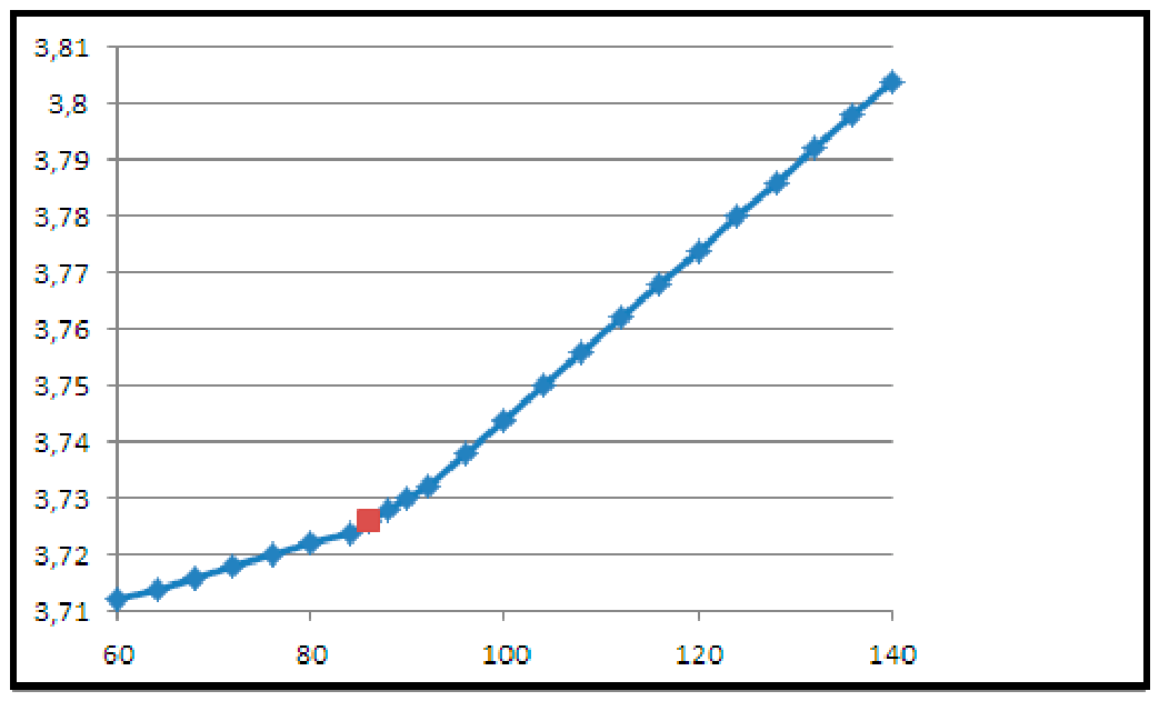
Figure 2.
Temperature dependence of the first peak height gmax for argon. The red square marks the transition temperature (Tm≈86K), where an inflection point is observed, indicating a change in the curvature of gmax (T).
Figure 2.
Temperature dependence of the first peak height gmax for argon. The red square marks the transition temperature (Tm≈86K), where an inflection point is observed, indicating a change in the curvature of gmax (T).
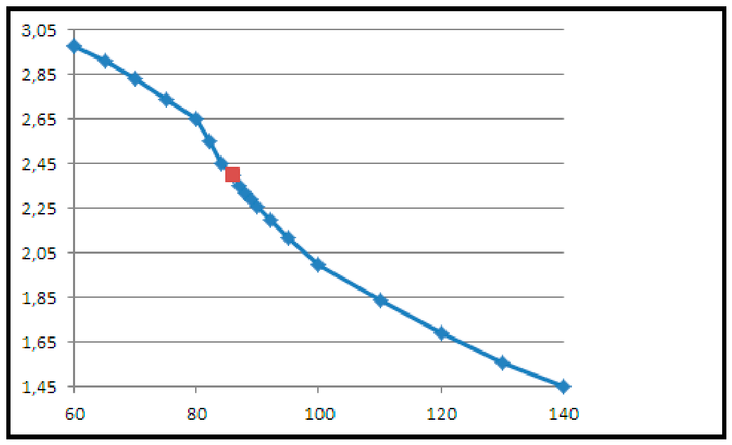
Figure 3.
Temperature dependence of the first peak width σ1 for argon. The red square marks the transition temperature (Tm≈86 K), where an inflection point occurs, indicating a change in the curvature of σ1(T).
Figure 3.
Temperature dependence of the first peak width σ1 for argon. The red square marks the transition temperature (Tm≈86 K), where an inflection point occurs, indicating a change in the curvature of σ1(T).
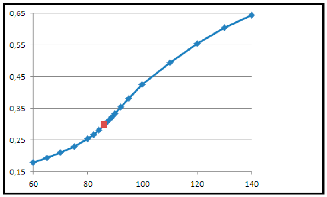
Figure 4.
Temperature dependence of the first well depth Umin of the PMF for argon. The red square marks the transition temperature (Tm≈86K), where a change in slope is observed.
Figure 4.
Temperature dependence of the first well depth Umin of the PMF for argon. The red square marks the transition temperature (Tm≈86K), where a change in slope is observed.
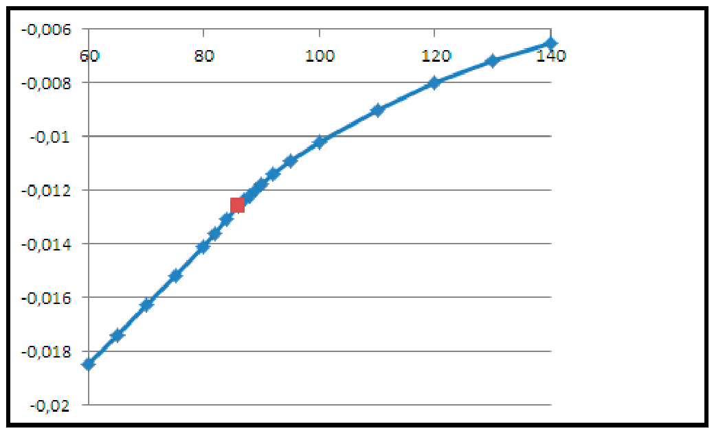
Figure 5.
Temperature dependence of the first eigenvalue μ1 of the Fisher equation for argon. The red square marks the transition temperature (Tm≈86K), where a change in slope and curvature is observed.
Figure 5.
Temperature dependence of the first eigenvalue μ1 of the Fisher equation for argon. The red square marks the transition temperature (Tm≈86K), where a change in slope and curvature is observed.
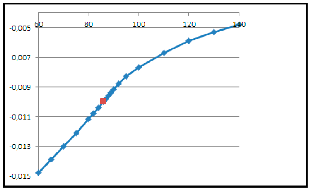
Figure 6.
Temperature dependence of the first peak position r1 for argon along the heating (solid → liquid) and cooling (liquid → solid) paths. The heating path (blue symbols) shows a transition near T≈86 K, while the cooling path (red symbols) shows a transition near T≈88 K.
Figure 6.
Temperature dependence of the first peak position r1 for argon along the heating (solid → liquid) and cooling (liquid → solid) paths. The heating path (blue symbols) shows a transition near T≈86 K, while the cooling path (red symbols) shows a transition near T≈88 K.
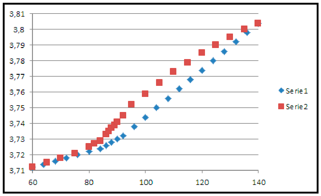

Table 1.
Estimated transition temperatures for heating and cooling paths, extracted from the temperature dependence of the structural and spectral parameters r1, gmax, σ1, Umin, and μ1. The transition temperatures are identified as the points where the parameters exhibit a change in slope, an inflection point, or a change in curvature. The hysteresis width ΔT=Tcooling−Theating quantifies the difference between the two paths, reflecting the first-order nature of the transition and the presence of metastable states (superheating of the solid and supercooling of the liquid). The average transition temperature is approximately 87.1 K, in good agreement with the experimental melting temperature of argon at 83.8 K. The consistent hysteresis observed across all parameters confirms the robustness of the spectral order parameter μ1 and the structural parameters in detecting the phase transition.
Table 1.
Estimated transition temperatures for heating and cooling paths, extracted from the temperature dependence of the structural and spectral parameters r1, gmax, σ1, Umin, and μ1. The transition temperatures are identified as the points where the parameters exhibit a change in slope, an inflection point, or a change in curvature. The hysteresis width ΔT=Tcooling−Theating quantifies the difference between the two paths, reflecting the first-order nature of the transition and the presence of metastable states (superheating of the solid and supercooling of the liquid). The average transition temperature is approximately 87.1 K, in good agreement with the experimental melting temperature of argon at 83.8 K. The consistent hysteresis observed across all parameters confirms the robustness of the spectral order parameter μ1 and the structural parameters in detecting the phase transition.
| Parameter | Symbol | Heating (K) | Cooling (K) | ΔT (K) |
| First peak position | r1 | 86.3 | 87.9 | 1.7 |
| First peak height | gmax | 86.3 | 87.9 | 1.6 |
| First peak width | σ1 | 86.0 | 88.0 | 2.0 |
| PMF well depth | Umin | 86.0 | 87.9 | 1.9 |
| First eigenvalue | μ1 | 86.0 | 88.0 | 2.0 |
Disclaimer/Publisher’s Note: The statements, opinions and data contained in all publications are solely those of the individual author(s) and contributor(s) and not of MDPI and/or the editor(s). MDPI and/or the editor(s) disclaim responsibility for any injury to people or property resulting from any ideas, methods, instructions or products referred to in the content. |
© 2026 by the authors. Licensee MDPI, Basel, Switzerland. This article is an open access article distributed under the terms and conditions of the Creative Commons Attribution (CC BY) license (http://creativecommons.org/licenses/by/4.0/).
Copyright: This open access article is published under a Creative Commons CC BY 4.0 license, which permit the free download, distribution, and reuse, provided that the author and preprint are cited in any reuse.