

Submitted:
31 August 2026
Posted:
09 September 2026
You are already at the latest version
Abstract
Studies of small-firm profitability estimate financial structure as the focal regressor and treat cost composition as an unexamined control. This paper reverses the emphasis and places both blocks in one equation, estimated on 91,756 firm-year observations covering 14,913 unlisted Italian firms across three regulatory regimes. Three methods interrogate different assumptions on the same sample: panel estimation across fourteen specifications, unsupervised partitioning selected on eleven validity criteria, and machine-learning regression applied to the same firm-demeaned data. The capitalisation coefficient is not identified. It moves from +0.177 under two-way fixed effects to between −0.12 and −0.28 under five instrument sets, all of which fail because profitability persists at 0.271, so any lagged financial ratio embeds past profit. The labour-share coefficient is stable across estimators, groups and functional forms, and the paper tests whether that stability is arithmetic, since return on assets and the labour share are consecutive lines of one statement. It is not: value added over total assets varies by a factor of 2.8 across the four operating archetypes recovered from the data, while the coefficient varies by 1.07. The accounting identity explains part of the magnitude and none of the stability.
Keywords:
SME profitability
; capital structure
; accounting identity
; instrument validity
; unsupervised classification
JEL codes: G32; L25; C23; C38; M41
1. Introduction
Why one small firm earns more than another is usually answered by reference to how it is financed. The literature on small and medium enterprises is organised around capital structure, and its central result is unusually stable: better capitalised firms are more profitable, as Matias and Serrasqueiro (2017), Dalci (2018), Quoc Trung (2021), Kalash (2023) and Youssef et al. (2023) establish across national panels. This paper asks a question the same data can answer but that has not been posed: when financial structure and the operating model are placed in one equation and measured on the same scale, which carries more of the variation in profitability?
The second term is almost absent from the literature that would have to answer it. Cost composition — the share of value added absorbed by labour, the intensity of purchased services, reliance on leased rather than owned capacity — enters firm-level profitability models as a control when it enters at all. The studies that do examine the operating side approach it through efficiency scores or working-capital ratios rather than through the composition of the cost base: Campisi et al. (2019), Grau and Reig (2021), Chadha et al. (2023) and Tripathi et al. (2024) are typical. The scarcity is measurable. Of 2,827 records retrieved from Scopus, twenty-seven relate labour cost, value added or outsourcing to firm profitability, against 447 relating capital structure to it. This is the first gap the study addresses.
The second is methodological. Endogeneity is treated as a nuisance corrected by internal instruments and reported in a robustness column, as in Canarella and Miller (2018), Vijayakumaran and Vijayakumaran (2019), Dsouza et al. (2025) and Saiz-Sepulveda et al. (2026). Two things are rarely acknowledged. Net worth contains the current year's profit and return on assets is computed on that profit, so part of any contemporaneous association is an accounting identity. And profitability is persistent — Hirsch and Hartmann (2014), Yang et al. (2015), Hirsch et al. (2021) and Choi et al. (2024) establish the regularity across settings — so any lagged financial ratio embedding past profit is correlated with the current error by construction. The persistence literature supplies the premise that invalidates the identification practice of the capital-structure literature, and the two strands rarely meet.
The third gap concerns the two literatures that could test the specification itself. Firm taxonomies built on accounting data, as in Linares-Mustarós et al. (2018), Juntunen et al. (2022) and Kristóf and Virág (2022), select partitions on a single validity index and describe the groups without re-estimating the relationship inside them. Machine learning on accounting data, as in Pap et al. (2022), Shetty et al. (2022), Vajjhala and Strang (2024) and Mahmood et al. (2025), is framed as prediction and evaluated on accuracy, with comparisons against linear models typically made on raw levels rather than on the transformation a fixed-effects estimator uses.
The originality of this study lies in holding one sample and one equation fixed while three methods interrogate different assumptions about it. The setting is the Italian population of certified innovative start-ups and innovative SMEs with a matched control of conventional firms — 91,756 firm-year observations on 14,913 firms — a regime whose evaluations, from Vannoni (2019), Manaresi et al. (2021), Migliaccio and Pavone (2021), Aiello et al. (2024), Anderloni and Harasheh (2025) and Scandurra et al. (2025), estimate average effects while presuming the mechanism. Panel estimation asks whether the association survives the estimator; unsupervised partitioning asks whether one coefficient vector describes every firm; machine-learning regression asks whether the linear form is adequate, on the same firm-demeaned data. The contribution is fourfold: the relative weight of the two blocks is measured within a single specification; the capitalisation coefficient is shown not to be identified by accounting data of this kind, and the reason diagnosed; the structure of profit determination differs across the regulatory populations the scheme defines; and machine learning is used diagnostically rather than competitively.
2. Literature Review
Two hundred studies were retrieved from Scopus and organised into eight themes. The corpus is recent — three quarters published since 2021 — and dominated by a design so standard that it can be described in one sentence: a national panel of firms observed over five to ten years, with a profitability ratio regressed on a capitalisation or leverage ratio and a set of controls, estimated by fixed effects or system GMM. What follows describes each theme, states what the design cannot answer, and locates the present study against it.
2.1. Capital Structure and Profitability in Small Firms
Whether the way a firm is financed shapes what it earns is among the most heavily worked questions in the empirical literature on small and medium enterprises, and its central result is unusually stable across settings. Matias and Serrasqueiro (2017) establish it for Portuguese firms, Dalci (2018) for Chinese manufacturers, Quoc Trung (2021) for Vietnam, Kalash (2023) for an emerging-market panel, Youssef et al. (2023) for non-financial UK SMEs, and Gonçalves et al. (2024), Bhawna and Sahay (2025) and Nkosi et al. (2026) for further national samples. Consistency of the sign conceals a real disagreement about why it holds. Under pecking-order reasoning, profitable firms accumulate retained earnings and borrow less, so causality runs from performance to structure; under trade-off and agency reasoning, leverage disciplines managers and the negative sign becomes a puzzle to be resolved by appeal to distress costs. Singh et al. (2025) and Demiraj et al. (2025) report evidence compatible with more than one mechanism, and the designs employed cannot separate them, because a single contemporaneous correlation is consistent with all of them. Three features of this literature bear on what follows. Samples are almost always listed or bank-financed firms. The equity or debt ratio is almost always the focal variable. And cost-structure variables, where they appear at all, enter as controls without discussion, so the question of whether financial structure matters more than the operating model is never posed.
2.2. Endogeneity, Simultaneity and Identification
The largest theme in the corpus is methodological in substance if not in title. Forty-six of the two hundred studies address endogeneity explicitly, most by instrumenting the focal regressor with its own lags or by moving to system GMM: Canarella and Miller (2018), Vijayakumaran and Vijayakumaran (2019), Samal and Yadav (2025), Dsouza et al. (2025) and Saiz-Sepulveda et al. (2026) are representative. The treatment is remarkably uniform. Endogeneity is acknowledged in a paragraph, an instrumented column is added to the robustness table, and the coefficient it produces is reported as confirming the main result. Instrument validity is tested in a minority of cases, and where a Hansen or Sargan statistic is reported it is almost never allowed to overturn the specification. Two consequences follow. Failures are invisible, because a paper whose instruments reject does not usually report them, so the literature contains no accumulated evidence on whether internal instruments work in this setting. And the specific mechanism that would invalidate them here is unacknowledged: net worth contains the current year's profit and return on assets is computed on that same profit, so part of any contemporaneous association is an accounting identity. Talamas Marcos (2025) and Rastogi and Kumar (2024) are among the few to exploit institutional variation rather than internal lags, and that approach has not become standard practice.
The reporting convention deserves comment in its own right. In this corpus the instrumented column is presented as a robustness check on a preferred fixed-effects estimate, which implies that the two are estimating the same parameter and that agreement between them is the expected outcome. When they disagree, the disagreement is usually attributed to instrument weakness and the fixed-effects estimate retained. That resolution is defensible only if the exclusion restriction is more likely to fail than the exogeneity of the regressor, and no paper in the corpus argues the point explicitly. The alternative reading — that neither estimate identifies the parameter and that the disagreement is the informative result — appears nowhere, though it follows directly from the diagnostics several of these studies already report.
2.3. Profit Persistence and Dynamic Adjustment
A separate literature establishes that profitability reverts towards a firm-specific mean at a measurable rate. Hirsch and Hartmann (2014) and Hirsch et al. (2021) document persistence in European food processing and retailing, Jaisinghani (2016) in Indian pharmaceuticals, Opstad et al. (2022) in restaurants, and Doyran and Santamaria (2019), Killins (2020) and Hoang et al. (2026) in banking and insurance. A parallel strand estimates the speed of adjustment towards a target capital structure — Yang et al. (2015), Sinha and Vodwal (2022), Choi et al. (2024), Abdeljawad and Farhood (2025) and Al Barakat and Ali (2026) — and reaches the same qualitative conclusion from the financing side. Both strands are technically careful and both use dynamic panel estimators. Neither, however, connects persistence to the identification problem of the previous theme, and the omission is consequential. If profitability at t is substantially predicted by profitability at t−2, and if the capitalisation ratio at t−2 mechanically embeds the profit of t−2, then lagged capitalisation is correlated with the current error by construction and cannot serve as an instrument. The persistence literature supplies the premise, the identification literature supplies the practice, and the two are rarely brought into contact.
2.4. Cost Structure, Efficiency and the Operating Model
The operating side of the firm enters the corpus through a different door. Grau and Reig (2021) study operating leverage in European agri-food SMEs, Campisi et al. (2019) and Alhassan and Ohene-Asare (2016) measure efficiency by data envelopment, Chadha et al. (2023) and Tripathi et al. (2024) examine working-capital efficiency in Indian MSMEs, and Bhattu-Babajee and Seetanah (2022) and Prasad and Mondal (2025) relate value added to performance. These are studies of efficiency, not of cost composition: they ask how well inputs are converted into output rather than how the cost base is divided between labour, purchased services, materials and leased capacity. The distinction matters because the second question can be answered from statutory accounts for the whole population of firms, and because the shares are the object a manager can act on. The scarcity is measurable. Of 2,827 records retrieved across eighteen queries, only twenty-seven relate labour cost, value added or outsourcing to profitability at firm level, against 447 relating capital structure to it. Where cost shares do appear in profitability regressions they are controls, reported without comment in a table whose discussion concerns the financial coefficient. No study in the corpus places the two blocks in one equation and asks which carries more of the variation.
2.5. Unsupervised Classification and Firm Taxonomies
Clustering enters the firm-level literature as description. Linares-Mustarós et al. (2018) classify firms by financial performance and distress profile, Juntunen et al. (2022) identify latent classes of accounting outsourcing firms, Ljungkvist and Andersén (2021) and Anton et al. (2021) build taxonomies of small manufacturers and of energy start-ups, Kristóf and Virág (2022) and Salina et al. (2020) partition sectors and banks on financial indicators, and Williams et al. (2025) and Bayaraa et al. (2019) combine clustering with efficiency analysis. Two limitations recur. The first is selection on a single index: silhouette is the default, and because it falls monotonically in the number of clusters for every partitional method, the procedure is biased towards coarse solutions before any substantive judgement is made. Papers reporting silhouette alone report two clusters; papers reporting partition R² alone report seven; the choice is presented as technical when it is in fact undetermined by the criterion. The second is that the partition is where the analysis stops. Groups are profiled and named, and their differences are described in means, but the estimating equation of the accompanying regression analysis is seldom re-estimated inside them, so the reader learns that firms differ without learning whether the pooled coefficients mean anything.
2.6. Machine Learning for Distress, Default and Fraud Prediction
The most established use of machine learning on accounting data is binary classification. Shetty et al. (2022), Gavurova et al. (2022), Papíková and Papík (2024), Cheraghali and Molnár (2026) and Bijoy et al. (2026) predict bankruptcy or distress; Zhang et al. (2025) and Sodnomdavaa and Lkhagvadorj (2026) predict fraud; Ariza-Garzón et al. (2024) and Antar and Tayachi (2025) add explainability tools to the same task. The methodological standard is high and the accuracy gains over logistic regression are consistent. The comparison with a parametric benchmark, however, is almost always conducted on raw levels, and this is where it becomes uninformative for an econometrician. A learner fitted to levels has between-firm variation available to it; a fixed-effects estimator does not. Setting one against the other attributes to functional form a difference that mostly reflects unmodelled firm heterogeneity, and the resulting statement that the learner is twice as accurate cannot be read as a verdict on the linear specification. The point applies with equal force to the continuous-outcome studies of the next theme, and correcting it changes the size of the gap by a factor of nearly three.
2.7. Machine Learning Applied to Firm Performance
A newer strand applies the same algorithms to continuous measures of performance. Pap et al. (2022), Vajjhala and Strang (2024), Garg et al. (2025), Mahmood et al. (2025) and Sultana et al. (2026) model profitability or organisational performance directly, Giudici et al. (2023) compare classification models, and Kristóf and Virág (2022), Vašaničová et al. (2025) and Coronell et al. (2026) combine supervised and unsupervised methods on financial ratios. These studies report accuracy rankings and, increasingly, variable-importance measures. What they do not do is turn the result back on the econometric specification. The gap between a linear model and an ensemble is reported as a reason to prefer the ensemble, not as a measurement of what the linear form omits, and it is not decomposed into components an econometrician could act on: curvature, interaction, or local structure that no polynomial reproduces. Nor is the gap located in the distribution, so it remains unknown whether a linear specification is inadequate everywhere or only in the tails. The tools for these questions — parametric enrichment, interaction statistics, permutation importance computed out of sample, decile calibration — are standard, and the corpus contains almost no example of their being used to validate rather than to replace a regression.
2.8. Innovative Start-Ups and Certified SMEs
The Italian certification regime has generated its own literature. Manaresi et al. (2021) evaluate the Start-up Act, Migliaccio and Pavone (2021) and Vannoni (2019) examine the financial structure of certified firms, Angilella et al. (2023), Aiello et al. (2024), Anderloni and Harasheh (2025) and Scandurra et al. (2025) compare certified firms with conventional peers, and Domma and Errico (2023), Schifilliti and La Rocca (2024) and Di Berardino and Antenozio (2026) study governance and digital orientation within the population. The dominant design is a treatment-effect comparison: certified firms against matched non-certified ones, with growth, employment, survival or access to finance as the outcome. The financing constraint the regime is meant to relieve is treated as given, and the question of whether profit is determined differently across the two populations is not usually asked. It is a different question from whether certified firms perform better on average, and fixed effects absorb the average difference entirely, leaving the structure of determination as the only thing that can still be compared. The regime also offers a natural test of any data-driven partition, since the register provides a classification the analyst did not construct, and no study in the corpus uses it that way.
2.9. Synthesis
Table 1 summarises the eight themes, the studies representing each, the gap each leaves, and what the present study contributes against it. Read down the third column, the gaps share a structure: each literature answers its own question competently and stops at the boundary where it would have to interrogate its own specification. The present study is organised around those boundaries rather than around a new dependent variable.
Three observations cut across the eight themes. The first is that sample composition is remarkably narrow: listed firms and bank borrowers dominate, and the unlisted micro and small firms that constitute the overwhelming majority of European enterprises appear mainly in survey-based work with short panels. The second is that method and question have drifted apart, with the econometric literature refining identification on a specification it does not test and the machine-learning literature testing specifications it does not interpret. The third is that the dependent variable is almost always taken as given, so the mechanical relationship between an accounting ratio and the regressors constructed from the same statements goes unexamined. The present study addresses the three together by holding one sample, one equation and one set of variables fixed across three methods that interrogate different assumptions.
2.10. Methodological Antecedents
The corpus assembled above is deliberately recent, and it inherits its questions from a body of work that predates it. Whether financial structure affects performance at all is the question Modigliani and Miller (1958) answered in the negative under conditions no small firm satisfies, and the departures from those conditions organise everything since: taxes and distress costs in the trade-off tradition, information asymmetry in Myers (1984) and Myers and Majluf (1984), agency costs in Jensen and Meckling (1976). The empirical regularities the recent panels reproduce were established by Titman and Wessels (1988), Rajan and Zingales (1995) and, for the small-firm case specifically, Berger and Udell (1998). Profit persistence has an equally settled pedigree in Mueller (1977), Geroski and Jacquemin (1988) and Fama and French (2000), whose mean-reversion estimates anticipate the autoregressive coefficient reported in Section 4.
The estimators are canonical and their diagnostics older than the applications that use them. The choice between fixed and random effects rests on Mundlak (1978) and Hausman (1978), with the variance test of Breusch and Pagan (1980); the bias that motivates a dynamic specification is Nickell (1981), and the instrumented first-difference estimator is Anderson and Hsiao (1981), generalised by Arellano and Bond (1991) and Blundell and Bond (1998). The overidentification statistic is Hansen (1982), and the weak-instrument literature that governs how a first-stage F should be read — and, more importantly, how it should not — is Bound et al. (1995), Staiger and Stock (1997) and Stock and Yogo (2005), whose warning that a large F reflects sample size as much as instrument strength is directly relevant to Appendix B. Inference clustered by firm follows Petersen (2009), and the multiway alternative discussed in Section 10 is Cameron et al. (2011).
The unsupervised and supervised tools are likewise inherited. The algorithms compared in Section 5 are MacQueen (1967), Ward (1963), Dempster et al. (1977), Bezdek (1981) and Ester et al. (1996); the validity criteria on which they are scored are Caliński and Harabasz (1974), Dunn (1974), Davies and Bouldin (1979) and Rousseeuw (1987), and the stability measure is the corrected index of Hubert and Arabie (1985). On the supervised side the learners are Breiman (2001) and Friedman (2001), and the interaction statistic used in Section 6 is Friedman and Popescu (2008). Naming these sources is not a formality: the silhouette coefficient favours coarse partitions by construction, and the first-stage F is not a measure of instrument strength in the sense that controls bias amplification. Both properties are stated in the original papers and lost in the applied literature that cites neither
3. Data and Methodology
The panel is assembled from thirty-one AIDA extractions covering the universe of Italian certified innovative start-ups and innovative SMEs together with a matched set of conventional small and medium enterprises. Each extraction reports 137 harmonised accounting variables replicated over ten financial years; the reference year of each column is reconstructed from the balance-sheet closing date, which is serialised differently across extractions. Regulatory status and sector codes are merged from the business register maintained by the Ministry of Enterprise, matched on fiscal code and added only after the accounting variables are built.
The estimating sample comprises 91,756 firm-year observations on 14,913 firms between 2014 and 2025, and it is identical across all three methods and all four appendices, so that differences between results are attributable to method rather than to sample.

Table 2.
Composition of the estimating sample.
| Population | Observations | Firms | Share of observations |
| Innovative start-ups | 12,864 | 5,173 | 14.0% |
| Innovative SMEs | 19,565 | 2,756 | 21.3% |
| Conventional SMEs | 59,327 | 6,995 | 64.7% |
| Total | 91,756 | 14,913 | 100.0% |
Note. Firm counts by population sum to slightly more than the total because eleven fiscal codes appear in two registers, having graduated from innovative start-up to innovative SME within the window; each is assigned to its earliest population.
The panel is unbalanced in a way correlated with regulatory status: start-ups file meaningful accounts in roughly one year in three against more than nine in ten for conventional SMEs, so conventional SMEs contribute close to two thirds of the observations while accounting for under half the firms. Appendix A establishes how much the weighting scheme matters.
The dependent variable is return on assets. The regressors form two blocks. The financial block comprises the equity ratio, the liquidity ratio, capital turnover and the logarithm of total assets; the operating block comprises the labour cost share of value added, purchased services and materials as proportions of the value of production, and payments for leased assets on the same basis. All continuous variables are winsorised at the first and ninety-ninth percentiles within year.
Two measurement decisions determine the sample. Cost ratios expressed against the value of production become uninformative where production approaches zero, so the sample is confined to observations with positive value of production, positive value added, and value of production of at least one per cent of total assets. The restriction removes 8.8 per cent of observations, but not neutrally: 29.3 per cent of start-up observations against 1.0 per cent of conventional ones, because pre-operating firms are concentrated among the certified. Rescaling the cost ratios on total assets is not an alternative, since return on assets carries assets in its denominator and the rescaled ratios would stand in an accounting identity with it — regressing ROA on the asset-scaled versions yields an R² of 0.488 against 0.088 for the output-scaled ones.
The equation is then estimated three times by methods that interrogate different assumptions: panel estimation, which tests whether the average association survives the choice of estimator and whether the equity ratio can be instrumented; unsupervised partitioning, which tests whether one coefficient vector describes every firm; and machine-learning regression, which tests the adequacy of the linear form on the same firm-demeaned data the fixed-effects estimator uses. Figure 1 sets out the design.
4. Panel Estimation
The equation relates return on assets to the four financial and the four operating regressors defined in Section 3. It is estimated by pooled OLS, by the between estimator on firm means, by fixed effects with firm dummies and with firm and year dummies, and by random effects; it is then put through four robustness treatments — weighted least squares under two weighting schemes, fixed effects with every regressor lagged one year, and a dynamic specification in first differences following Anderson and Hsiao (1981). Standard errors are clustered by firm in every specification. The five static estimators use the full 91,756 observations on 14,913 firms; the lagged and the dynamic specifications lose the opening years of each firm's series and fall to 76,261 and 64,031 observations respectively. Sample, variable definitions and winsorisation are held fixed across every column, so that what differs between columns is the estimator and nothing else.
Which estimator serves as the reference is settled by test rather than by preference, and the three tests that settle it interrogate different nulls.
Table 4.
Panel structure tests.
| Test | Statistic | p | Conclusion |
| F(uᵢ = 0), two-way FE | 5.60 | < 0.0001 | Pooled OLS rejected |
| Breusch–Pagan LM | 25,011.2 | < 0.0001 | Individual variance present |
| Hausman (FE vs. RE) | 117.01 | < 0.0001 | Random effects inconsistent |
| First-stage F (Anderson–Hsiao) | 18,229.8 | — | Instrument strong |
Note. Hausman on eight degrees of freedom. The first-stage F refers to ROA(t−2) as instrument for the lagged difference in the dynamic specification ofTable A2.
The F statistic asks whether firm effects exist at all; the Breusch–Pagan multiplier asks whether their variance is non-zero; the Hausman statistic asks whether they are correlated with the regressors. Rejecting the first two without the third would license random effects, which are the more efficient estimator and are widely used in this literature on precisely that ground. Rejecting all three closes the route and fixes two-way fixed effects as the reference specification. Table 3 reports it, with the between and the firm-only fixed-effects columns set alongside so that the two comparisons that matter most can be made without turning to the appendix.
All eight regressors are significant at the one per cent level, and the within R² of 0.4232 indicates that the specification accounts for a substantial share of the variation in profitability that occurs inside firms over time. The coefficients cannot, however, be compared with one another as they stand, because the regressors are measured on incompatible scales: a unit of capital turnover and a percentage point of the labour share are not comparable quantities, and reading the column downwards would make turnover appear to dominate by a factor of thirty. Figure 2 therefore rescales every coefficient to the effect of a one-standard-deviation increase, which places all eight on the single axis of percentage points of ROA.
Capital turnover dominates under every estimator and the labour share follows immediately. A one-standard-deviation increase in turnover is worth approximately four points of ROA and a comparable increase in the labour share costs close to four; capitalisation is worth about three; purchased services, materials and leased assets between one and two points each; liquidity is negligible throughout. The financial and the operating block therefore contribute on the same order of magnitude, which the unrescaled coefficients of Table 3 conceal entirely, and the ordering is unchanged across the four estimators plotted. What the Figure Aannot show is the difference between the two sources of variation those estimators exploit, which Figure 3 isolates by plotting the between and the within estimate as a pair for each regressor.
The comparison of between with within is more informative than any single coefficient, and it is the diagnostic least often reported in this literature. On the labour share and on purchased services the two estimates almost coincide, and the natural reading — that a relationship holding both across firms and inside them over time is structural rather than compositional — is the wrong one here. An accounting relation holds in both dimensions indifferentially, since it is a property of how the statements are constructed and not of how firms behave, so coincidence of the two estimates is the first trace of the identity examined in Section 7 rather than evidence against it. The diagnostic retains its value, but with the sign of its interpretation reversed: what would be informative on the labour share is divergence, not agreement. The other two comparisons are unaffected, because neither variable enters the identity. On size the two estimates diverge sharply and change sign, so within-firm asset growth operates differently from the advantage of being structurally large; liquidity changes sign in the same way and is small in both dimensions. Capitalisation is higher within than between, which is what the mechanical component of that coefficient would predict and is not evidence of a stronger structural effect.
That objection is elementary and the literature reporting a positive capitalisation coefficient rarely confronts it. Net worth contains the current year's profit, and return on assets is computed on that same profit, so part of the association is an accounting identity rather than an economic relationship. The objection is raised here because it bears on the coefficient this section traces, but it is not confined to it: four of the eight regressors are ratios of an item subtracted in the income statement to the aggregate it is subtracted from, and the operating block is exposed to it more severely than the financial one. Section 7 develops the point in full and revises the reading of the operating coefficients accordingly; what follows should be read in that light.
Three treatments separate identity from relationship, and they do not agree with one another. Lagging every regressor by one year reverses the sign, from +0.177 to −0.068, with significance unchanged. Modelling persistence instead — first differences with ROA(t−2) instrumenting the lagged difference, in the manner of Anderson and Hsiao — returns the coefficient to positive and larger than the static estimate at +0.228, with an autoregressive parameter of 0.271 and a first-stage F of 18,230. Instrumenting the equity ratio directly, across five instrument sets, produces a negative estimate in every case. Figure 4 places all fourteen specifications on a single axis.
The figure is the finding. The five static estimators cluster between +0.12 and +0.18 and the two weighted variants stay within that band; lagging moves the coefficient below zero; the dynamic specification moves it back above every static estimate; each instrumental-variable specification places it between −0.12 and −0.28. These are not overlapping confidence intervals around a common parameter but qualitatively different answers to the same question, and no ranking of the estimators by their own diagnostics resolves the disagreement, because the specifications that reverse the sign are precisely the ones designed to address the identity problem. The sign of the capitalisation coefficient is not identified by these data, and that instability is the result rather than an obstacle to it.
The operating coefficients behave in the opposite way — across seven of the eight estimators the labour share ranges only between −0.115 and −0.141, and the ranking of the four operating variables never changes — but the contrast is not the one it first appears to be, and Section 7 takes it up in full. Return on assets and the labour share are consecutive lines of the same income statement, so an estimator-invariant coefficient is what that construction produces and cannot be read, without further test, as evidence of a relationship more robust than the financial one. What the comparison does establish is an asymmetry worth stating plainly here: the equity ratio is not mechanically determined by the cost base and its sign is nonetheless unidentified, while the labour share is mechanically related to the outcome and stable for that reason. Of the two, the literature has organised itself around the variable whose association with performance is the weaker and the less reliably signed.
The instrumental-variable estimates are reported in full in Appendix B rather than here, because they fail on their own terms and a failed identification strategy does not belong in the body of the argument. All five instrument sets are strong: first-stage F statistics run from 24 for the province-year peer mean to 2,327 for the second lag of the equity ratio. Strength is not validity, and the overidentified specification using the second and third lags rejects the Hansen test with a statistic of 77.18. The mechanism of failure is identifiable rather than merely suspected: with ROA persistent at 0.271, the equity ratio at t−2 mechanically embeds profit at t−2, which predicts profit at t through persistence alone, so the exclusion restriction fails by construction and no lag length escapes it while profitability remains persistent. The one instrument with a defensible exclusion restriction, net external equity injections, is too weakly related to the regressor to be usable: its within-firm correlation with the equity ratio is 0.103, which amplifies any violation of exclusion roughly tenfold. Reporting the attempt with its diagnostics forecloses an obvious referee request and is more informative than omitting it.
Two further features of the panel bear on how the coefficients should be read. The panel is unbalanced in a way correlated with regulatory status, so the weighting scheme determines whose experience the estimates describe. Weighting each firm equally rather than each observation raises capitalisation from 0.177 to 0.199 and size from 0.646 to 0.855, so the relationship is somewhat stronger among firms observed briefly. Weighting by total assets instead, which recovers the coefficient relevant to the economic aggregate rather than to the median firm, halves capitalisation to 0.099 while raising capital turnover from 5.29 to 6.89 and materials from −0.114 to −0.149. In the firms that carry the aggregate the operating model matters more and financial structure less. Neither weighting is correct in the abstract; the two answer different questions and both are reported in Table A2.
The second feature is that a single coefficient vector has been imposed on three populations that the regulation itself treats as distinct. Estimating the equation separately by regime, on the same observations and the same specification, tests that restriction directly, and Figure 5 plots the three vectors on the standardised scale of Figure 2.
Wald tests reject equality of the coefficient vectors in all three pairwise comparisons: 87.18 between start-ups and innovative SMEs, 181.94 between start-ups and ordinary SMEs, and 138.08 between the two SME categories, each on eight degrees of freedom with p below 10⁻⁴. What differs is not the level of profitability, which the fixed effects absorb, but the structure of its determination. Capital turnover carries a coefficient of 7.02 among start-ups and 7.35 among innovative SMEs against 4.17 among ordinary SMEs, while the labour share weighs most heavily on ordinary SMEs at −0.163; capitalisation is highest among start-ups at 0.232. Certification schemes rest on the premise that innovative firms operate under constraints different from those facing conventional ones, and evaluations customarily measure average effects on growth or employment while treating the constraint as given. The evidence here is that the difference is measurable in the structure of the profit equation itself and survives every specification attempted. It also motivates Section 5, which asks whether the partition that matters is the regulatory one or one the data would choose for themselves.
5. Unsupervised Structure
The panel estimates of Section 4 impose a restriction the data have not been asked to confirm: that a single coefficient vector describes every firm. The restriction can be tested without leaving the equation, by partitioning firms on the equation's own variables and re-estimating within each partition. What the exercise can establish is whether the pooled coefficients mean what they appear to mean or whether they average structures that differ; what it cannot establish is any causal effect, and no claim of that kind is made here. The partition is a description of coefficient heterogeneity, and it is built from accounting variables alone.
Each firm is summarised by the decade median of the nine variables entering the equation, standardised to zero mean and unit variance, on the same 14,913 firms and the same 91,756 observations used in Section 4. Regulatory status is withheld from the procedure entirely and used afterwards only as an external check, so that any correspondence between the partition and the register is a result rather than an assumption. Thirty-two configurations were evaluated across six algorithm families — k-means, Ward agglomerative, Gaussian mixture and fuzzy c-means for k between two and seven, density-based clustering over five radii, and random-forest proximity clustering for k between two and four — of which twenty-nine returned a partition with at least two groups; the three discarded are density-based solutions at the widest radii, where every firm falls into a single component. Each retained configuration was scored on eleven validity criteria: silhouette, Calinski–Harabasz, Davies–Bouldin, Dunn, maximum diameter, minimum separation, the Pearson gamma between distances and co-membership, entropy, the Herfindahl–Hirschman index of cluster balance, partition R², and, where defined, the Bayesian information criterion.
Selecting on any single index misleads, and the direction of the error is systematic rather than random. Silhouette falls monotonicatablely in k for every partitional method, so on that criterion alone the two-cluster solution always wins; Calinski–Harabasz behaves identically. Partition R² and the Dunn index move in the opposite direction, rewarding finer partitions. A paper reporting silhouette alone would therefore report two clusters, and a paper reporting R² alone would report seven, from the same data and the same algorithm. The two density-based configurations attain the highest silhouette values in the entire battery while classifying between four and thirty-three per cent of firms as noise, which is what a high silhouette means when a procedure is free to discard the observations that fit badly. Averaging ranks across the nine directional indices selects k-means at k = 4: it places first on partition R² among the balanced solutions and keeps its smallest group at 14.9 per cent of firms. Fifty bootstrap resamples at eighty per cent give a mean adjusted Rand index of 0.9375 with a minimum of 0.6167, so the partition is not an artefact of the particular sample. The neighbouring three-cluster solution ranks immediately behind and was estimated in full as a robustness check; the coefficient pattern reported below survives it.
The four groups are best read on the standardised scale, where each cell states how far a group's typical firm lies from the sample mean in standard deviations.
Figure 6.
Cluster profiles, standardised means.
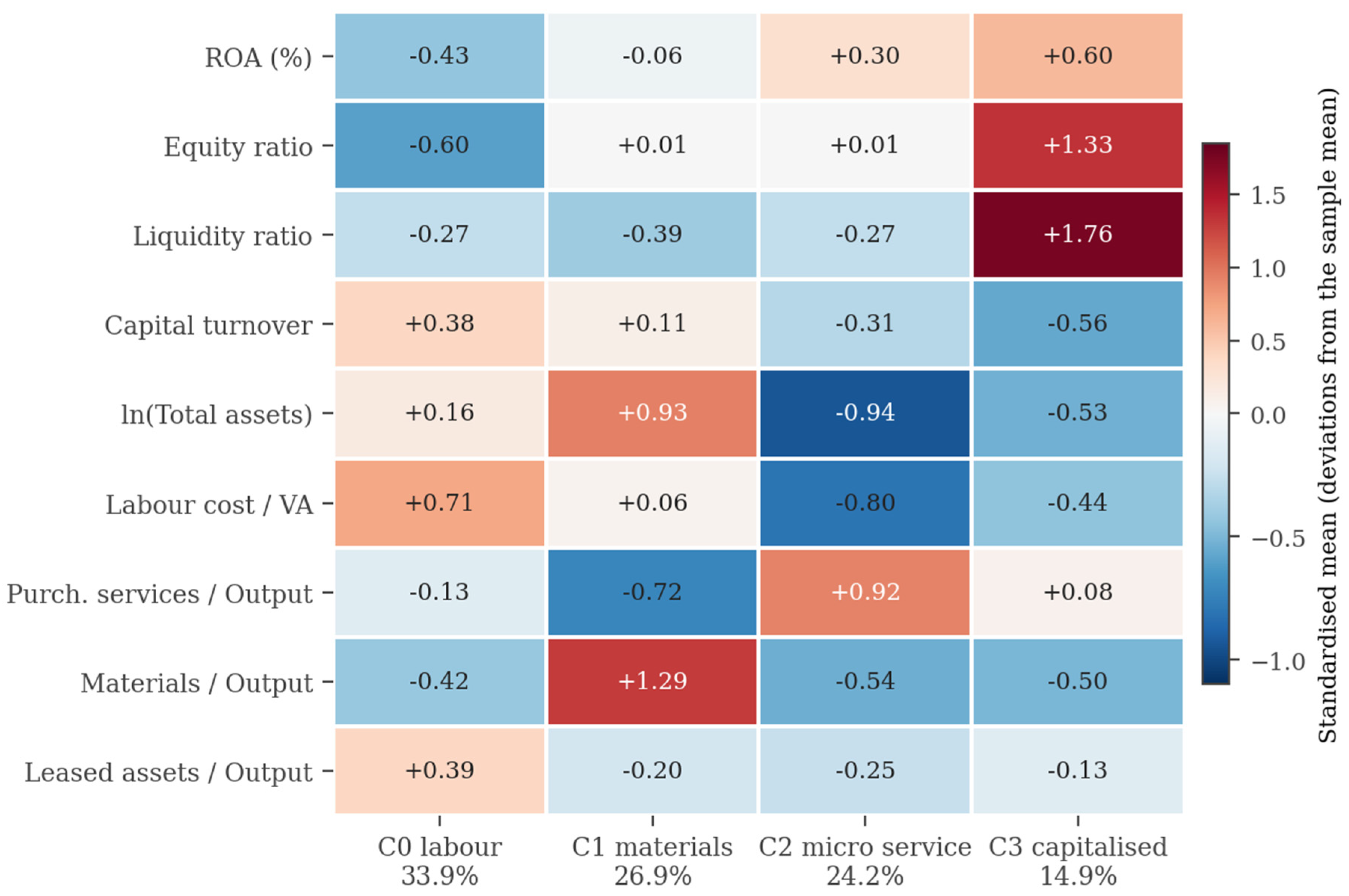
The colours identify the archetypes and the medians in Table 5 give them their magnitudes in the units of the accounts. Cluster 0, a third of all firms, is labour-intensive: a labour share of 89.6 per cent of value added, the lowest capitalisation in the sample at 17.3 per cent, and the lowest median return at 3.03. Cluster 1, twenty-seven per cent, is materials-intensive and the largest in scale, with materials at 47.4 per cent of output and median log assets of 9.75. Cluster 2, twenty-four per cent, is composed of micro service firms: purchased services at 57.4 per cent of output, a labour share of 0.63 per cent, the smallest scale in the sample and a median return of 7.36. Cluster 3, fifteen per cent, is the only group defined financially rather than operationally, with capitalisation of 70.1 per cent, a liquidity ratio of 3.70, the lowest capital turnover and the highest median return at 10.23.
Two features of the separation matter more than the labels. The first is that the financial variables behave differently from the operating ones in how they organise the partition. Capitalisation and liquidity are extreme in Cluster 3 and virtually identical across the other three groups, at 0.01, 0.01 and −0.60 standard deviations for the equity ratio: they identify one archetype sharply and say almost nothing about the remaining eighty-five per cent of firms. The labour share and purchased services, by contrast, take a distinct value in each of the four groups and order them. Financial structure characterises an archetype; it does not organise the partition. The second is that the partition was formed without reference to profitability being a target, yet median ROA rises monotonically across the four groups from 3.03 to 10.23, which is the first indication that these are not merely descriptive categories.
Regulatory status was withheld from the procedure, so the correspondence between the partition and the register is an external test of both.
Figure 7.
Cluster composition by regulatory regime.
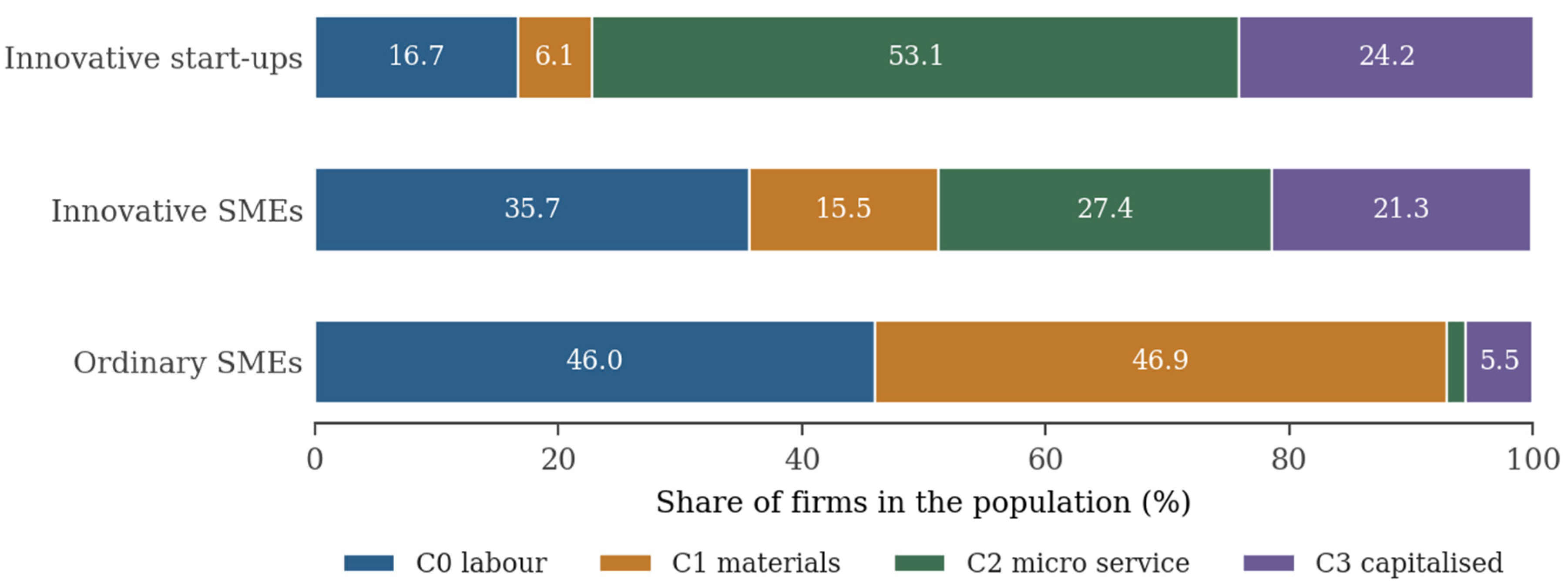
Partition and register correspond strongly without coinciding: χ²(6) = 6,821.9 with Cramér's V of 0.4780. Ordinary SMEs concentrate almost entirely in the two established operating archetypes, 46.0 and 46.9 per cent, with only 7.1 per cent elsewhere. Innovative start-ups distribute almost inversely, 53.1 per cent in the micro-service group and 24.2 per cent in the capitalised one, which is what the certification regime would predict for firms that are small, service-oriented and recently equity-funded. Innovative SMEs spread across all four groups, consistent with a category reached either by graduation from start-up status or by direct entry from conventional activity. The regulatory categories therefore carry real information about the operating model, but they are not the same partition: a Cramér's V of 0.478 leaves a great deal of the variation unexplained, and the analysis of Section 4 by regime and the analysis here by archetype are answering different questions.
The point of the partition is what happens when the equation is re-estimated inside it. The same specification, the same estimator and the same observations are used; only the grouping changes.
Table 6.
Equation re-estimated within each cluster (selected coefficients).
| Regressor | C0 labour | C1 materials | C2 micro service | C3 capitalised |
| Capital turnover | 3.0860*** | 5.9623*** | 7.8726*** | 13.1552*** |
| (0.1742) | (0.2216) | (0.3498) | (0.6774) | |
| Labour cost / Value added (%) | -0.1403*** | -0.1317*** | -0.1347*** | -0.1383*** |
| (0.0038) | (0.0047) | (0.0061) | (0.0084) | |
| Purchased services / Output (%) | -0.0980*** | -0.1510*** | -0.2475*** | -0.2852*** |
| (0.0075) | (0.0139) | (0.0155) | (0.0176) | |
| Leased assets / Output (%) | -0.1909*** | -0.2800*** | -0.3051*** | -0.4937*** |
| (0.0234) | (0.0505) | (0.0390) | (0.0545) | |
| Equity ratio (%) | 0.2314*** | 0.1015*** | 0.2002*** | 0.1280*** |
| (0.0091) | (0.0069) | (0.0104) | (0.0136) | |
| Observations | 34,377 | 34,632 | 12,804 | 10,062 |
| Within R² | 0.4293 | 0.4955 | 0.4420 | 0.4759 |
Note. Two-way fixed effects, firm-clustered standard errors in parentheses. *** p<0.01. The full eight-regressor estimates are Table A5.
Pairwise Wald tests reject equality of the coefficient vectors for all six pairs, with statistics between 84.45 and 374.34 on eight degrees of freedom. Rejection at this sample size is not by itself informative, since almost any restriction is rejected on ninety thousand observations; what matters is the magnitude and the pattern of the differences, which Figure 8 shows by expressing each within-cluster coefficient as a multiple of the pooled estimate from Table 3.
The two remaining dimensions are stable for opposite reasons. Liquidity is insignificant in three groups of four, so the pooled estimate is right that it does not matter anywhere. The labour-share coefficient varies by a factor of only 1.1, lying between −0.132 and −0.140 with overlapping confidence intervals throughout, and invariance of that kind invites an obvious objection: return on assets and the labour share are consecutive lines of the same income statement, so a coefficient that does not move across groups may be recording a construction rather than a relationship. The objection is taken up in Section 7 and it carries a testable implication, because the identity fixes the slope at −VA / A: a coefficient this close to constant across archetypes requires value added over total assets to be close to constant across them as well.
It is not. Value added over assets ranges from 0.217 in the micro-service cluster to 0.602 in the labour-intensive one, a factor of 2.8, against a factor of 1.07 in the coefficient. The invariance therefore survives the test that would have exposed it as arithmetic, and it survives it on a partition constructed from the very variables that generate the arithmetic. Of the eight dimensions of the pooled vector, one is faithful because the underlying relationship really is common to all four groups, one is faithful because the variable is inert everywhere, and on the remaining six the pooled estimate averages quantities that differ by factors of two to four.
The ordering of the equity-ratio coefficient is worth isolating, because it is the coefficient Section 4 could not sign. Within clusters it is positive everywhere, but it is weakest in the materials-intensive group of larger firms at 0.102 and strongest in the labour-intensive group of smaller, thinly capitalised ones at 0.231 — the pattern a financing-constraint reading predicts, with capitalisation mattering most where it is scarcest. That is a pattern, not an identification, and it does not resolve the instability documented in Figure 4; the accounting identity operates inside each cluster exactly as it does in the pooled sample. What the partition adds is that the pooled coefficient of 0.177 is not merely uncertain in sign but heterogeneous in magnitude, so that the specification search of Section 4 was conducted on a parameter that does not have a single value.
Two implications follow for how the rest of the paper reads. The first is that the regulatory partition tested in Section 4 and the operating partition tested here are both real and neither is the other: certification tracks the operating model strongly enough to produce a Cramér's V of 0.478 but not so strongly that policy categories can substitute for cost structure in an empirical model. The second is that the linear specification has now been questioned in one direction only. Section 5 has asked whether one coefficient vector fits every firm and answered that it does not; it has not asked whether the coefficients are constant within a group, or whether the relationship between each regressor and profitability is linear at all. That is the question Section 6 addresses, on the same observations, by fitting learners that impose no functional form and measuring what they recover that the linear equation does not.
6. Machine-Learning Regression as Validation
The panel specification rests on two assumptions beyond those already tested. Section 5 examined the first, that a single coefficient vector describes every firm, and rejected it. The second is that each regressor enters linearly and additively. Examining that one requires estimators that impose no functional form and can therefore be asked how much of the variation in profitability a linear equation leaves unexplained. The purpose here is validation rather than prediction: nothing in this section forecasts profitability, no learner replaces the equation, and no coefficient is revised on the strength of a fit. The questions are how large the gap between the linear form and an unrestricted one is, what kind of structure accounts for it, and whether the ordering of variables implied by the panel coefficients survives an independent measure of predictive content.
Thirteen algorithms were fitted to the same 91,756 observations on the same eight regressors, with five-fold cross-validation grouped by firm so that no firm contributes to both the training and the test partition. They were compared on out-of-sample R², the cross-fold standard deviation of that R², root mean squared error, mean absolute error and fitting time, reported in full as Table A1. Selection follows the same principle as the clustering of Section 5: a battery rather than a single index. Histogram gradient boosting attains the highest accuracy at 0.7978, the lowest errors at 5.932 and 3.476, and a cross-fold standard deviation of 0.0070 among the lowest in the battery, in 3.3 seconds against 120.5 for the random forest that comes third on accuracy. It is used for every result that follows. The comparison also has a finding of its own: the thirteen algorithms fall into three bands rather than a continuum, with tree ensembles and the neural network above 0.72, k-nearest neighbours and the single decision tree between 0.64 and 0.70, and the entire linear family, including the linear support-vector machine, below 0.48.
The comparison that matters is nevertheless not that one, because it is the comparison most often made incorrectly. The fixed-effects estimator explains variation within firms, after firm means have been removed; a learner fitted to raw levels also has the between-firm variation available to it. Setting a within R² of 0.42 against a levels R² of 0.80 therefore attributes to functional form what mostly reflects a different decomposition of the variance. The comparison is made three times instead, under three treatments of the between-firm information.
Table 7.
Like-for-like comparison of linear and non-linear fits.
| Data transformation | Linear R² | SD | Gradient boosting R² | SD | Gap | Ratio |
| Levels (pooled) | 0.4730 | 0.0112 | 0.7978 | 0.0070 | 0.3248 | 1.69x |
| Firm-demeaned (within) | 0.4153 | 0.0126 | 0.5360 | 0.0107 | 0.1206 | 1.29x |
| Levels + firm means (Mundlak) | 0.4795 | 0.0116 | 0.7986 | 0.0054 | 0.3191 | 1.67x |
Note. Five-fold cross-validation grouped by firm. SD is the standard deviation of R² across folds. The second row applies to both models exactly the transformation the fixed-effects estimator applies.
The three rows answer the same question under three different treatments of between-firm variation, and reading them together is what makes the comparison interpretable. The first gives the learner access to differences between firms as well as within them. The second removes firm means, replicating exactly what the fixed-effects estimator does. The third restores the between-firm information to the linear model in the form of firm means, following Mundlak. Comparing the first with the third isolates how much of the linear model's apparent disadvantage on levels is simply unmodelled firm heterogeneity; comparing the second with either isolates what remains attributable to functional form.
Figure 9.
Out-of-sample accuracy under three transformations.
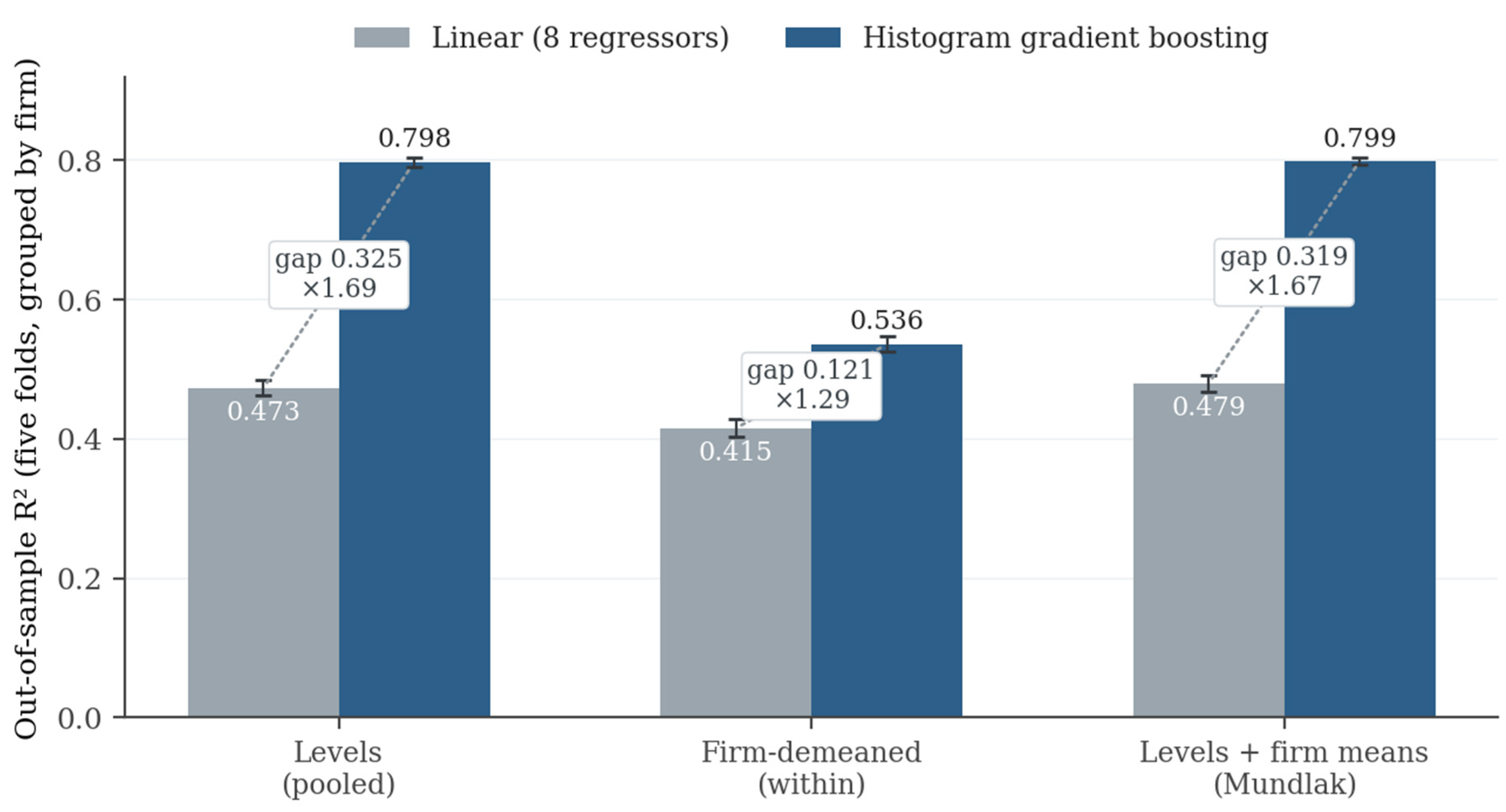
On raw levels the non-linear model is 1.69 times more accurate. On firm-demeaned data, which is what the fixed-effects estimator uses, the ratio falls to 1.29 and the absolute gap from 0.325 to 0.121: the linear specification recovers 0.415 of within-firm variance against 0.536 attainable. Supplying the linear model with firm means in the manner of Mundlak raises it only from 0.473 to 0.480, which locates the source of the remaining difference: on levels the learner's advantage is mostly firm heterogeneity that fixed effects already absorb, and what survives the demeaning is functional form. The honest statement of the gap is therefore 0.121 rather than 0.325, and everything that follows concerns those twelve points of R².
The next question is what kind of structure they represent, and the first candidate is one the linear model can be given directly. If the missing structure were polynomial, adding squares and interactions to the equation would recover it, at a cost in parameters that can be counted.
Table 8.
How much of the gap parametric terms recover.
| Specification | Terms | R² | SD | Gap closed (%) |
| Linear, 8 regressors | 8 | 0.4153 | 0.0126 | 0.0 |
| + squared terms | 16 | 0.4319 | 0.0116 | 13.7 |
| + pairwise interactions | 36 | 0.4355 | 0.0125 | 16.7 |
| + squares and interactions | 44 | 0.4401 | 0.0114 | 20.6 |
| Full cubic expansion | 164 | 0.3672 | 0.1890 | -39.9 |
| Histogram gradient boosting | — | 0.5360 | 0.0107 | 100.0 |
Note. Firm-demeaned data, five-fold cross-validation grouped by firm. Gap closed is the share of the 0.1206 difference between the linear specification and gradient boosting that each enrichment recovers.
The table turns each specification into a price, and the figure shows what is bought.
Figure 10.
Parametric enrichment against gradient boosting, firm-demeaned data.
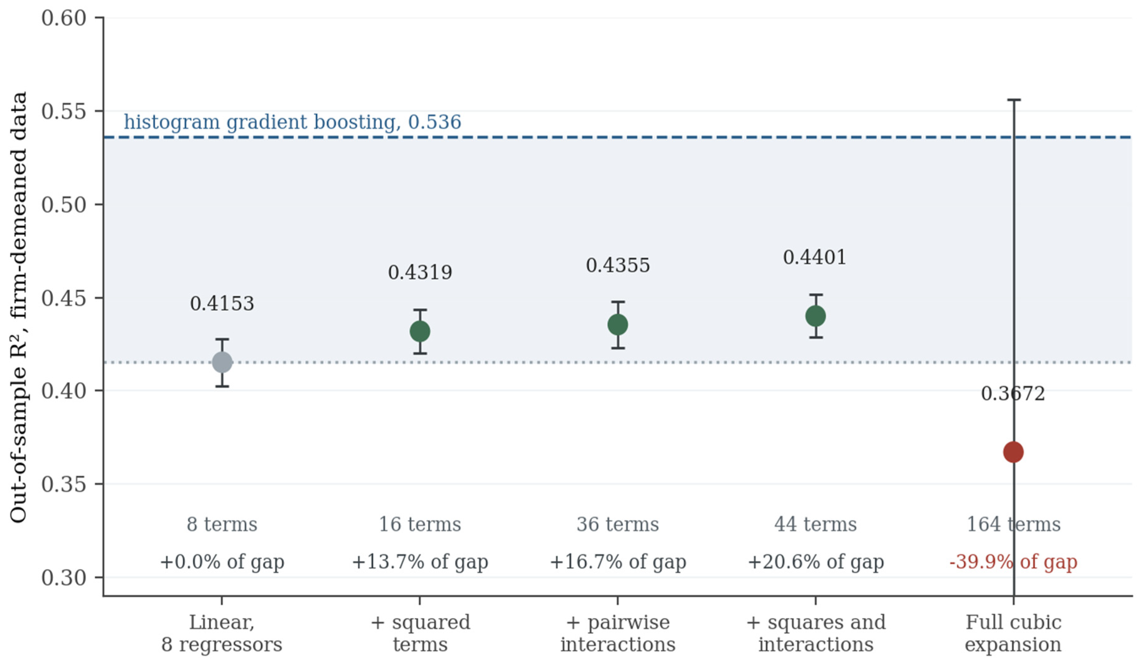
Sixteen terms buy 13.7 per cent of the gap, forty-four buy 20.6, and one hundred and sixty-four buy nothing at all: the full cubic expansion performs worse than the original eight-regressor model, with a cross-fold standard deviation of 0.189 against 0.013, because it overfits the tails of a heavy-tailed dependent variable. The cross-fold standard deviation is the column that explains the failure rather than merely recording it, and it is why the cubic row is reported at all. Roughly four fifths of what the learner captures is therefore not polynomial. Nor is it interaction: Friedman H-statistics are small throughout, the strongest pair — the equity ratio with capital turnover — reaching 0.042, so the residual structure is univariate curvature rather than joint dependence between regressors. What the linear form omits is local structure: thresholds, saturation, and regions of a variable's range where it matters against regions where it does not.
Partial dependence makes those shapes explicit and explains why polynomials approximate them badly. The labour share declines steeply over its lower range and then flattens, so its marginal effect is concentrated among firms whose wage bill is a moderate share of value added and close to nil among those where it is already dominant. Capital turnover rises and saturates. Purchased services are flat over most of their range before bending at the upper end. The equity ratio is close to monotone and mild, which is consistent with the modest positive fixed-effects coefficient rather than with the negative instrumental-variable estimates of Section 4. A quadratic term must curve everywhere in order to curve anywhere, and a cubic must reverse; the surface the learner recovers is instead flat in some regions and steep in others, which is exactly the structure a low-order polynomial cannot represent and a tree ensemble represents naturally.
A second question is independent of fit. Permutation importance measures how much out-of-sample accuracy is lost when a predictor is randomly reshuffled, so it ranks variables by contribution to genuine prediction rather than by coefficient magnitude or by significance, and it is computed on held-out data.
Figure 11.
Permutation importance, firm-demeaned data.
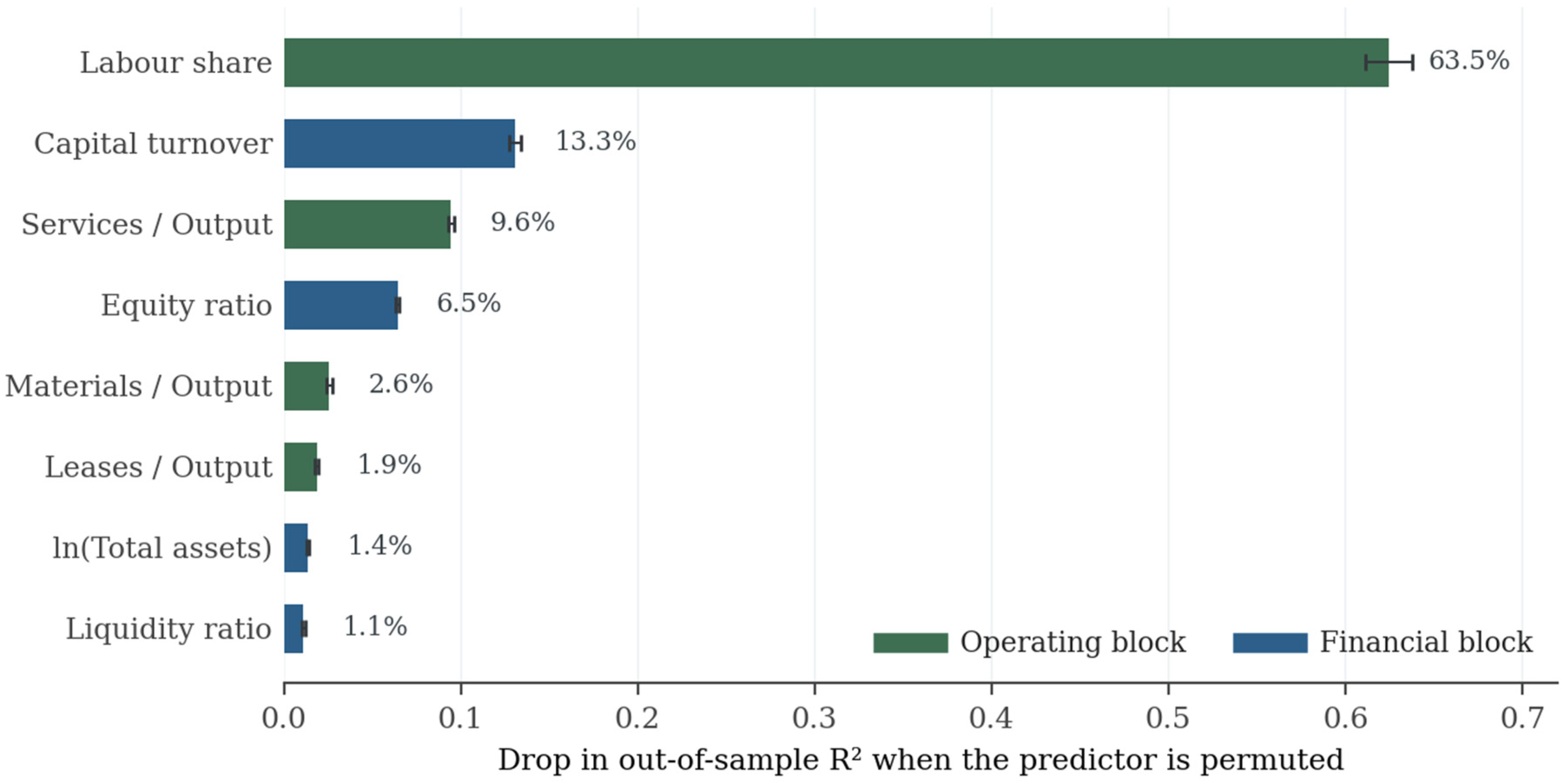
The labour share alone accounts for 63.5 per cent of predictive content, capital turnover for 13.3 and purchased services for 9.6. The operating block carries roughly ninety per cent of the information, against 6.5 per cent for the equity ratio and 1.1 for liquidity, and the error bars are small relative to the distance between the labour share and everything else, so the ordering is not a sampling artefact. This is a sharper hierarchy than the panel coefficients suggest — Figure 2 put capitalisation and the labour share within a point of one another on the standardised scale — and it is reached by a route that uses no standard errors and no functional form.
The interpretation of the leading entry requires the qualification developed in Section 7, and stating it here rather than there prevents the figure from being read as a third independent confirmation. A learner recovers an accounting relation almost perfectly, and return on assets and the labour share are consecutive lines of one income statement, so a substantial part of the 63.5 per cent measures the predictive content of a construction rather than of a behaviour. The permutation exercise agrees with the panel estimates and with the clustering because all three inherit the same arithmetic, not because three independent routes converge. What the Figure Aoes establish independently is the position of capital turnover, which enters no identity and which the panel coefficients understate: second on this measure at 13.3 per cent, and the variable whose coefficient varies most across archetypes. And the entry that is informative by its smallness is the equity ratio, at 6.5 per cent, since capitalisation is not mechanically tied to the outcome and its low share is therefore a statement about explanatory content rather than about construction.
The last diagnostic asks where in the distribution the two models differ, which a single R² cannot show.
Figure 12.
Calibration by decile of realised profitability.
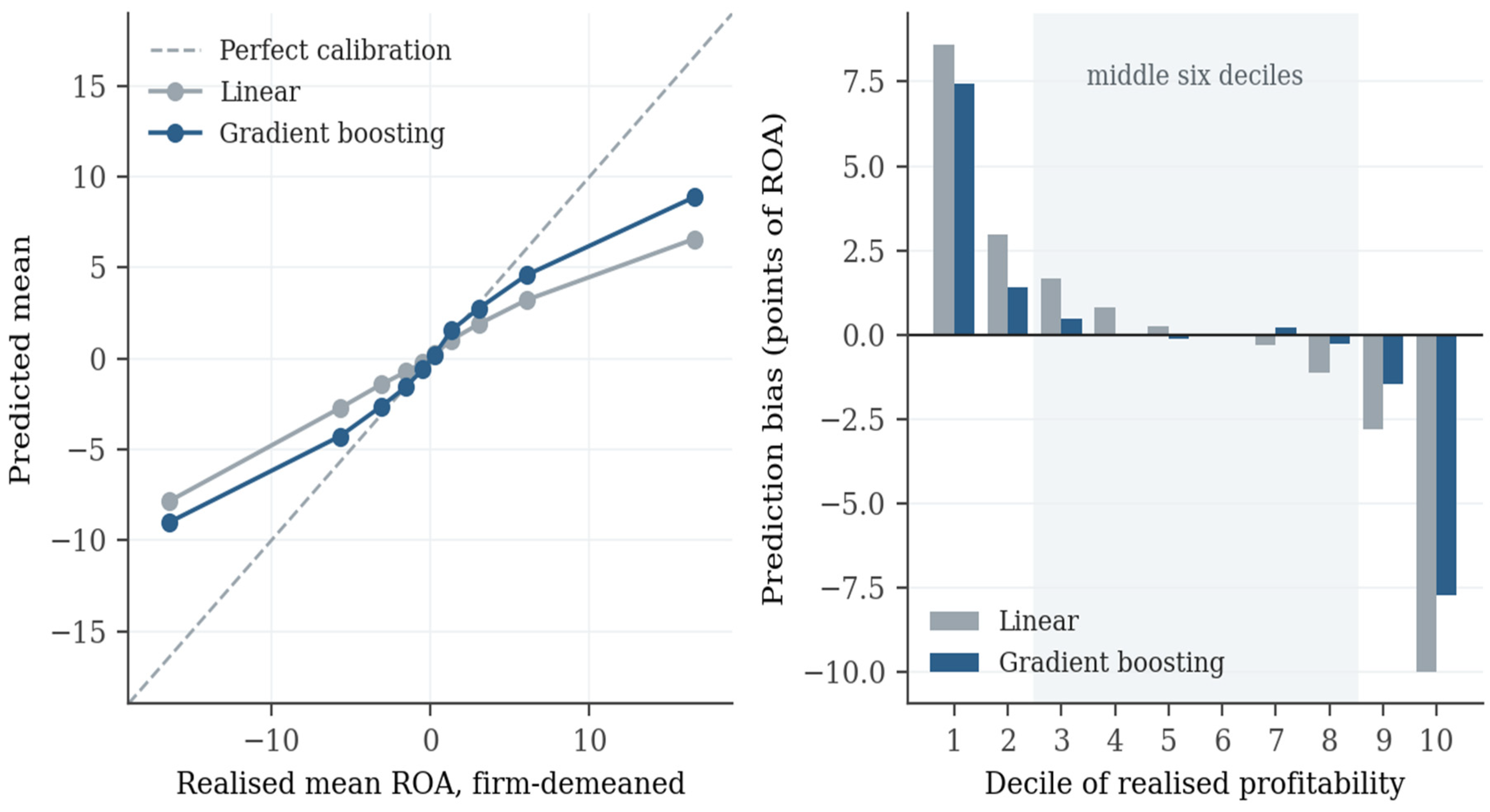
In the bottom decile of demeaned ROA, where the realised mean is −16.5 points, the linear model predicts −7.9; in the top decile, realised at +16.6, it predicts +6.6. The linear model compresses the distribution towards its centre by roughly a factor of two at the extremes, and gradient boosting by a factor of 1.8, so the non-linear model is better calibrated in the tails without being well calibrated there. In the middle six deciles both are accurate, with biases below 1.7 points and below 0.5 for four of the six. Essentially the whole difference between the two specifications arises in the two deciles at each end, which is worth stating explicitly because it identifies exactly which observations drive the result: a study that trimmed the tails would find the linear and the non-linear specification nearly equivalent, and would be right about the firms it retained and silent about the rest.
Three conclusions follow for the panel estimates, and they are conclusions about interpretation rather than about validity. The coefficients of Section 4 are local linear approximations to a mildly curved surface and should be described as average slopes rather than as constant marginal effects, with the approximation weakest for the most and least profitable tenths of the sample. The ranking of variables they imply is corroborated rather than overturned by an independent measure of predictive content, and corroborated by a wider margin than the coefficients themselves suggest. And the residual gap is not a matter of sample size: the learning curve of Appendix D shows the linear model flat from the first ten thousand observations, its test score rising from 0.4005 to 0.4153 over a twenty-fold increase in training data, while the boosting test score converges towards 0.536 from above. What the linear specification lacks is form, not information, and the twelve points of R² it cannot reach set a realistic ceiling for any equation of this kind estimated on these variables.
7. The Accounting Identity in the Operating Block
The argument of Section 4 against the capitalisation coefficient applies with greater force to the coefficient this paper reports as its main finding, and the objection is best raised here rather than answered defensively later. Net worth contains the current year's profit, which is why the equity ratio stands in a partly mechanical relationship with return on assets. The labour share of value added stands in a relationship that is mechanical by construction, because the two quantities are consecutive lines of the same income statement.
Figure 13.
Where the regressors sit in the income statement that generates the dependent variable.
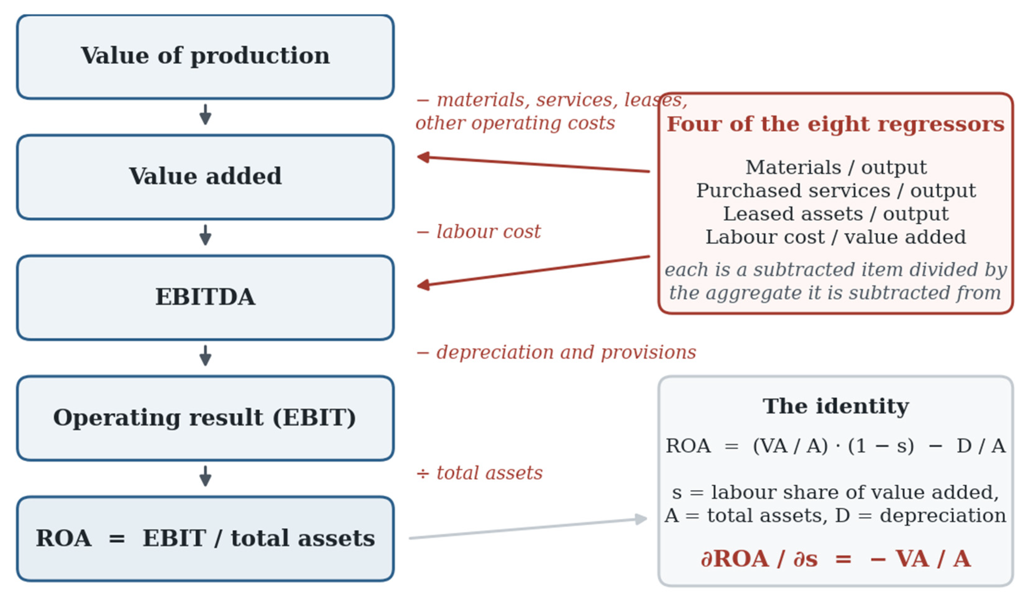
Under the Italian civil-code scheme, value added is the value of production less materials, purchased services, leased assets and other operating costs; EBITDA is value added less labour cost; and the operating result is EBITDA less depreciation and provisions. Writing s for the labour share and A for total assets, ROA = (VA / A)(1 − s) − D / A. The derivative of the dependent variable with respect to the regressor is therefore −VA / A exactly, before any estimation. Four of the eight regressors are ratios of an item subtracted in that cascade to the aggregate it is subtracted from, so the operating block as a whole is exposed to the objection, and the labour share most of all.
Two readings advanced earlier in the paper have to be withdrawn as a consequence. The stability of the labour-share coefficient across estimators, reported in Section 4 as evidence that the relationship is structural, is what an accounting relation produces, since such a relation does not depend on the estimator. And its 63.5 per cent share of permutation importance measures in part the predictive content of a construction rather than of a behaviour, since a learner recovers an identity almost perfectly. A third reading looks like the same point in another form — the near-invariance of the coefficient across the four clusters, at −0.132 to −0.140 — and Section 7.1 shows that it is not. The reason the three can be told apart is that the identity fixes not only the sign of the coefficient but its magnitude, and magnitude is checkable.
7.1. How Much of the Coefficient Is Mechanical
The identity predicts a slope of −VA / A, so the test requires one quantity the estimating equation does not report: the distribution of value added over total assets in the sample itself.
Table 10.
Value added over total assets in the estimating sample.
| Population | p5 | p10 | p25 | Median | p75 | p90 | Mean | Obs. |
| All firms | 0.055 | 0.105 | 0.211 | 0.353 | 0.604 | 1.040 | 0.498 | 96,052 |
| Innovative start-ups | 0.015 | 0.031 | 0.088 | 0.213 | 0.435 | 0.727 | 0.321 | 14,412 |
| Innovative SMEs | 0.034 | 0.066 | 0.156 | 0.304 | 0.515 | 0.753 | 0.370 | 20,907 |
| Ordinary SMEs | 0.130 | 0.174 | 0.257 | 0.394 | 0.697 | 1.256 | 0.584 | 60,733 |
Note. Value added and total assets as reported in the statutory accounts, winsorised at the first and ninety-ninth percentiles. The ratio is not among the nine variables of the estimating equation and was therefore computed separately, by reapplying the sample construction of Section 3 to the source extractions: positive value of production, positive value added, and value of production of at least one per cent of total assets. The resulting 96,052 firm-year observations on 15,501 firms exceed the estimating sample of Table 2 by 4.7 per cent, because the ratio requires only two of the nine variables and is defined for firm-years that the full specification drops for missingness elsewhere. The difference is not selective on any dimension relevant to the comparison: the median of the ratio changes by less than 0.01 when the sample is restricted to firm-years with all nine variables present.
The median is 0.353 and the middle half of the sample lies between 0.211 and 0.604. The identity therefore predicts a coefficient of about −0.355 for the median firm and between −0.21 and −0.60 for the interquartile range. The estimated coefficient is −0.1365.
Figure 14.
The distribution of value added over total assets, and the slope the identity implies.
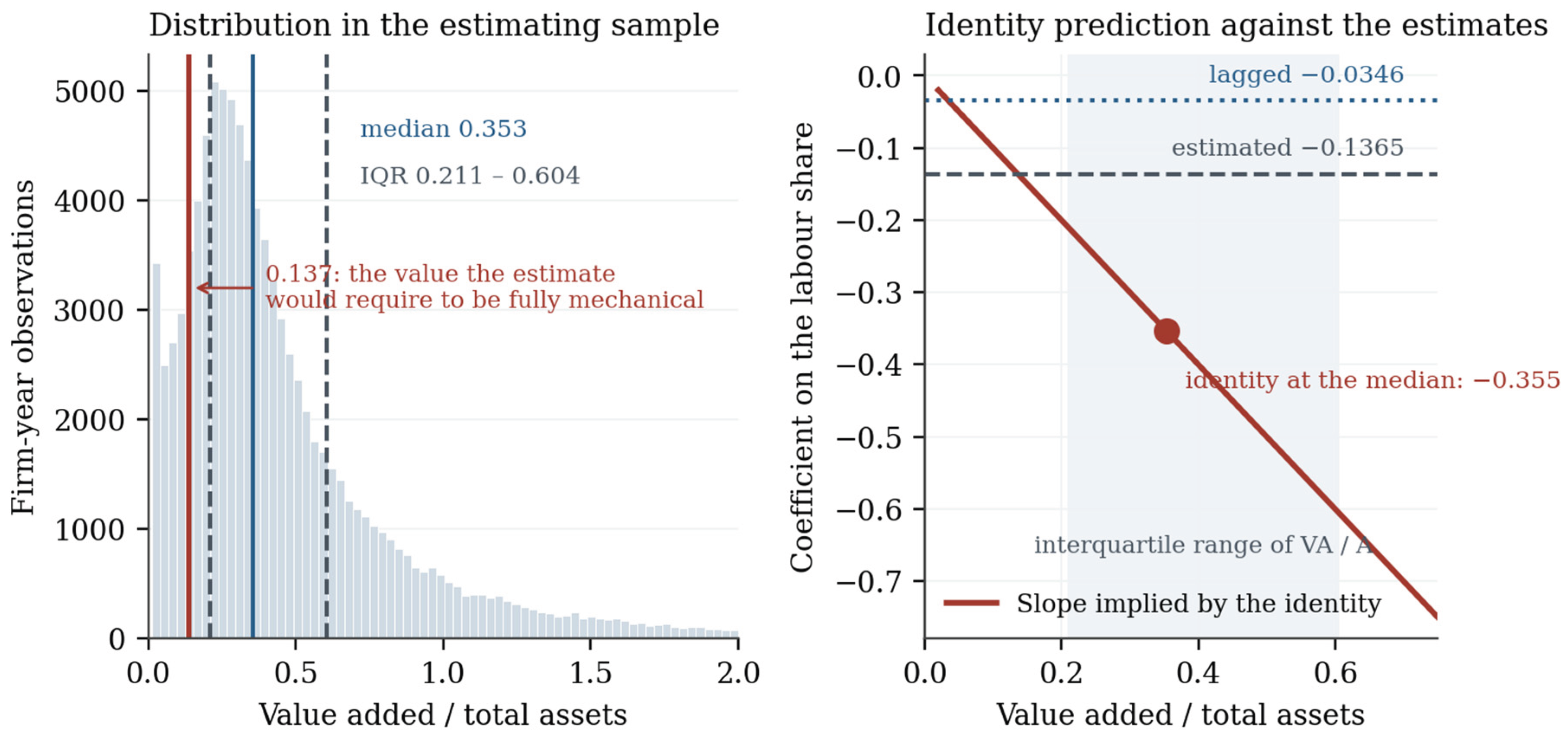
The estimate is not the identity. It is roughly two-fifths of the magnitude predicted at the median and falls below the first quartile of the predicted range. For the coefficient to be mechanical in full, value added would have to be 13.7 per cent of total assets, and just under fourteen per cent of firm-years are at or below that level — concentrated among start-ups, whose median is 0.213 against 0.394 for ordinary SMEs. The identity is unmistakably present in these data, and it over-predicts what is estimated by a factor of between two and three.
Two mechanisms account for the gap and both can be quantified. The first is conditioning. The equation includes capital turnover, revenue over assets, which absorbs much of the variation in value added over assets, so the reported coefficient is a partial effect holding scale intensity fixed rather than the unconditional slope the identity describes. The second is the covariance between the labour share and value-added intensity within firms: regressing VA / A on the labour share with firm effects returns a slope of −0.00068, so a firm whose labour share rises by ten points sees value added over assets fall by 0.007, and the total derivative implied by the identity moves from −0.355 to −0.375 at the median, and to −0.283 when firms are weighted by the within-firm variance of the labour share that the fixed-effects estimator actually exploits. Neither adjustment brings the prediction near −0.1365.
A second and independent comparison is already available in the estimates of Section 4. Lagging every regressor by one year breaks the identity, because the labour share of t−1 and the profit of t are computed from different statements. What survives the break bounds from below whatever part of the coefficient is not contemporaneous arithmetic.
Figure 15.
What survives when the identity is broken by lagging.
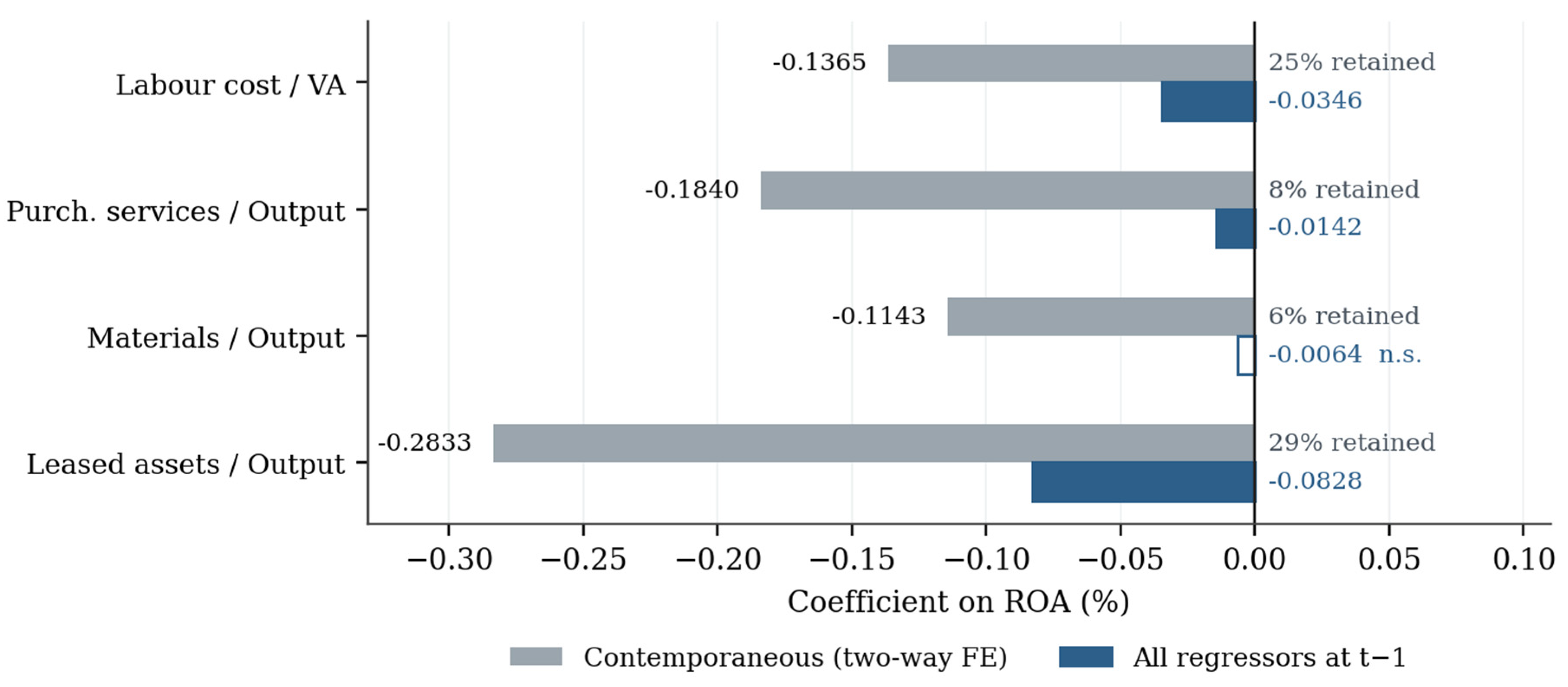
The labour share retains a quarter of its magnitude at −0.0346 and remains significant at one per cent; leased assets retain 29 per cent, purchased services 8 per cent, and materials become insignificant. The retained quarter would require a value added of 3.5 per cent of total assets to be mechanical in its turn, a level reached by 3.2 per cent of firm-years, so the lagged coefficient is unlikely to be an artefact of construction. It is not, however, a clean estimate of behaviour either, since lagging also changes the question a cost structure is being asked to answer: it predicts next year's profit rather than this year's, and some of the loss is dynamics rather than arithmetic.
A third comparison settles the matter, and it uses the partition of Section 5 rather than the time dimension. The identity fixes the slope at −VA / A, so it predicts not one magnitude for the sample but a different magnitude for every group of firms whose value-added intensity differs. The four archetypes differ in that respect considerably: median value added over total assets runs from 0.217 in the micro-service cluster to 0.602 in the labour-intensive one, a factor of 2.8. If the coefficient were mechanical it would have to vary by the same factor, and be largest in absolute value precisely where value added per unit of assets is largest.
They do not. Across the four archetypes the predicted slope ranges by a factor of 2.8 and the estimated coefficient by a factor of 1.07, from −0.132 to −0.140, with confidence intervals that overlap throughout. The ordering is partially preserved — the labour-intensive cluster does carry the largest coefficient in absolute value, as the identity requires — but the amplitude is not, and amplitude is what the identity fixes. The ratio of estimate to prediction falls from 0.62 in the micro-service cluster to 0.23 in the labour-intensive one, so the attenuation is itself systematic, and largest exactly where the mechanical component should be strongest.
Figure 16.
The identity prediction against the estimate, by archetype.
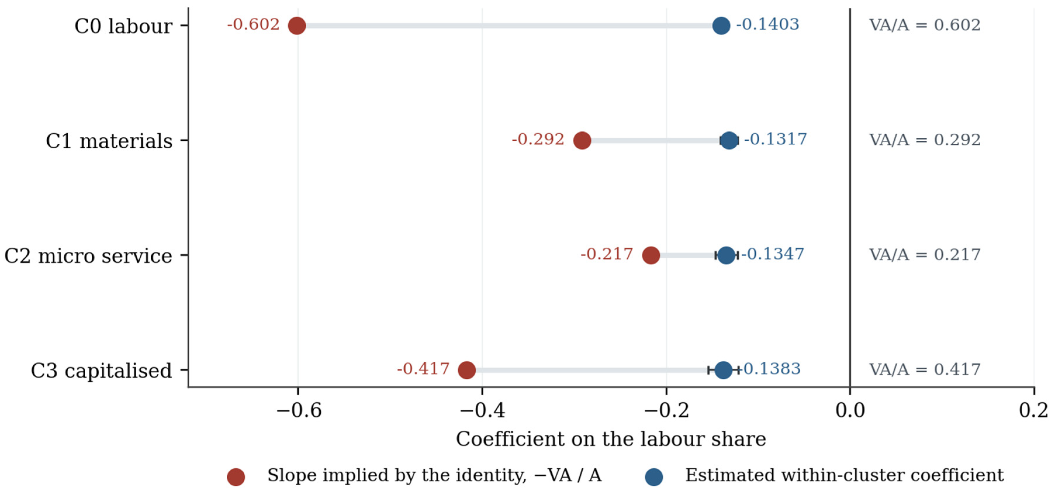
This is the decisive comparison of the three, because it holds the identity fixed and varies the quantity the identity says the coefficient must track. A relation that is arithmetic cannot be near-constant across groups whose multiplier differs threefold. The near-invariance reported in Section 5 is therefore not the signature of an accounting relation after all: it is a property of the estimated relationship, and it survives a partition built to separate firms on exactly the dimensions that generate the arithmetic.
The three comparisons can be stated together. The contemporaneous coefficient is smaller than the identity alone would generate, so it is the identity net of the variation the specification conditions away; the lagged coefficient survives a break in the identity, so a part of the association is not contemporaneous arithmetic at all; and the coefficient is stable across groups in which the identity's multiplier is not, so its stability is not mechanical either. The identity is present in these data, it accounts for part of the level of the coefficient, and it accounts for neither its stability nor the whole of its magnitude.
7.2. What the Contribution Becomes
The paper's claim changes in wording rather than in value, and the honest statement of it is this. A large share of the observed variation in return on assets is fixed once the composition of the cost base is known, and part of that share is arithmetic rather than behavioural. This is a measurement the literature reviewed in Section 2 has not reported and which policy has proceeded as though it did not exist, and it is sharper for being bounded on both sides: the identity over-predicts the coefficient by a factor of two to three, and a quarter of the association survives the breaking of the identity altogether.
The comparison with financial structure survives the concession intact and is sharpened by it. The equity ratio is not mechanically determined by the cost base, and its coefficient is unstable in sign across fourteen specifications and identified by no instrument these data admit. The labour share is mechanically related to profitability, and part of its stability follows from that relation — but only part, since the stability itself survives a test the identity fails. A literature that has organised itself around the first variable while treating the second as a control has therefore chosen, of the two, the one whose association with performance is both weaker and less reliably signed. That claim requires no causal interpretation of either coefficient.
The clustering and machine-learning results are affected asymmetrically. The dispersion of the capital-turnover coefficient by a factor of 4.3 across archetypes is untouched, since turnover enters no identity, and it remains the strongest evidence in the paper that a single coefficient vector does not describe every firm. The invariance of the labour-share coefficient, which Section 7 opened by treating as suspect, emerges from Table 12 as a finding rather than an artefact. Only the machine-learning ceiling of 0.536 is qualified: a learner approaches an accounting relation closely, so part of the within-firm predictive accuracy it attains is the identity, and the informative residual is what it recovers beyond that.
Two of the five tests that would separate identity from relationship remain open, and both require re-estimation on the present sample rather than new data. They are listed for completeness and because the direction each would have to take is already specified.
Table 11.
Five tests that separate identity from relationship.
| Test | Identity predicts | Structure predicts | Status and result | What it establishes |
| Coefficient equals −VA / A | Equality | Departure from −VA / A | Done. Identity implies −0.355 at the median and −0.283 to −0.375 under alternative weightings; estimate is −0.1365 | The estimate is the identity attenuated, not the identity itself |
| Lagged regressors | Coefficient near zero | Coefficient survives | Done. −0.0346***, a quarter retained; would require VA / A of 0.035, reached by 3.2% of firm-years | A lower bound on the non-mechanical component |
| Slope tracks VA / A across clusters | Coefficient varies with cluster VA / A | Coefficient invariant while VA / A varies | Done. VA / A ranges 2.8× across archetypes, the coefficient 1.07×, from −0.132 to −0.140 | The stability of the coefficient is not mechanical |
| Dependent variable VA / A, labour share as regressor | No association | Association survives | Outstanding. Re-estimation only, same variables and sample | Whether the labour share predicts a quantity it does not enter |
| ROA at t + 1 on labour share at t | Coefficient near zero | Coefficient survives | Outstanding. Re-estimation only, one year of observations lost | Predictive content free of the shared statement |
Note. The first test uses Table 10 and the two-way fixed-effects estimate of Table 3; the second uses the lagged specification of Table A2; the third uses Table 12. The remaining two require re-estimation on the sample of Section 3 and no new variables. Shading distinguishes completed tests from outstandin.
8. Discussion
Three methods were applied to one sample, and the value of doing so lies in where they agree and where they do not. On the operating block they agree: the labour share carries the largest standardised coefficient after capital turnover, varies by a factor of only 1.1 across the four clusters, and accounts for 63.5 per cent of out-of-sample predictive content. Agreement of that kind invites an obvious objection, since an accounting relation also holds whatever the estimator, the subsample or the functional form, and Section 7 tests it rather than conceding it. The identity turns out to explain part of the level of the coefficient and none of its stability: it predicts −0.355 at the median firm against an estimate of −0.1365, and it predicts a threefold variation across archetypes where the estimates vary by seven per cent. What the three methods converge on is therefore a relationship that is partly arithmetic in magnitude and not arithmetic in its constancy.
On financial structure the three methods disagree, and the disagreement is informative rather than a defect. The static panel estimates reproduce the sign reported by Matias and Serrasqueiro (2017), Dalci (2018), Kalash (2023) and Youssef et al. (2023): better capitalised firms earn more. Lagging the regressors reverses that sign, the dynamic specification restores it, and every instrument set contradicts both. Because net worth contains the current year's profit, part of the contemporaneous association is mechanical here too, and because profitability persists at 0.271 no lag length escapes the problem — which is why the internal instruments used by Vijayakumaran and Vijayakumaran (2019), Dsouza et al. (2025) and Saiz-Sepulveda et al. (2026) fail. The persistence documented by Hirsch and Hartmann (2014) and Hirsch et al. (2021) and the identification practice of the capital-structure literature are, on this evidence, incompatible.
Setting the two blocks side by side is what the paper can claim without any causal interpretation. The equity ratio is not mechanically determined by the cost base, and its coefficient is unstable in sign across fourteen specifications and identified by no instrument these data admit. The labour share is mechanically related to profitability, yet its coefficient is more stable than that relation alone would produce and remains constant where the relation predicts it should move. Of the two variables, a literature organised around the first has chosen the one whose association with performance is both weaker and less reliably signed, while treating the second as a control — which is the position of Campisi et al. (2019), Grau and Reig (2021), Bhattu-Babajee and Seetanah (2022) and Chadha et al. (2023), none of whom place the blocks in competition.
The clustering and machine-learning results are affected asymmetrically. Capital turnover enters no identity, so its dispersion by a factor of 4.3 across archetypes is a failure of the pooled vector and the strongest evidence that one coefficient set does not describe every firm. The partition earns a second role beyond description, since it is what makes the identity testable: groups that differ in value-added intensity are groups in which a mechanical coefficient would have to differ. The 0.536 ceiling on within-firm predictive accuracy, by contrast, is partly an artefact of the same arithmetic, because a learner approaches an accounting relation closely, and the interesting residual is what it recovers beyond that. Both results qualify the panel estimates without overturning them, which is the sense in which the exercise is validation rather than replacement — a use of these algorithms that the prediction-oriented applications of Pap et al. (2022), Vajjhala and Strang (2024) and Mahmood et al. (2025) do not attempt.
Two implications for practice follow. For the empirical literature, the appropriate response to an unsTable Aoefficient is to report the instability rather than to select the treatment that preserves the expected sign; and the appropriate response to a stable one is to test whether the stability is arithmetic before reading it as structure, which requires only that the identity be written down and its prediction compared with the estimate. The corpus reviewed in Section 2 contains no instance of either check, in either direction. For policy, the certification regimes evaluated by Manaresi et al. (2021) and Scandurra et al. (2025) rest on relieving a financing constraint whose measured association with profitability cannot be signed on this population, while the cost margin that does carry the association receives no instrument at all.
Table 9 states, for each method, what was found and whether it aligns with, qualifies, or contradicts the existing evidence.
9. Policy Implications
Italy's productive structure is dominated by firms that do not grow: the size distribution is compressed towards the bottom, and the number of firms making the transition from micro to medium scale in any decade is small. This is habitually treated as a financing problem, and the policy instruments in place are built accordingly. The evidence assembled here bears on that diagnosis directly, and four implications follow.
The first concerns what certification schemes are for. The Italian Start-up Act, like most European equivalents, presumes that innovative firms are constrained by access to capital and responds with tax relief on equity investment, free access to a public credit guarantee, and relief from company-law rules on capital maintenance. Evaluations by Manaresi et al. (2021), Aiello et al. (2024), Anderloni and Harasheh (2025) and Scandurra et al. (2025) establish that the instruments reach their targets and improve financing outcomes. What the present results add is that the constraint they relieve is not the one that binds on profitability. Capitalisation accounts for 6.5 per cent of out-of-sample predictive content and cannot be signed reliably; the share of value added absorbed by labour accounts for 63.5 per cent and is stable across every estimator, every group and every functional form tried. A firm whose cost structure leaves no margin does not become profitable because equity is cheaper.
The second concerns the sixty-month horizon. Certification expires by statute five years after incorporation, which presumes that firms reach a stable operating configuration within that window. The partition recovered in Section 5 suggests otherwise: 53.1 per cent of certified start-ups sit in a micro-service configuration with a labour share close to zero and the lowest capital turnover in the sample, and the coefficient vector governing their profitability differs significantly from that of established operating firms. Migliaccio and Pavone (2021) and Vannoni (2019) document the same internal heterogeneity from the financial side, and Tran and Santarelli (2014) and Amoa-Gyarteng and Dhliwayo (2023) report comparable patterns for young firms elsewhere. A fixed horizon applied to a population this heterogeneous withdraws support from firms at very different stages of development.
The third concerns instruments that act on the price of capital. Italian firms remain overwhelmingly bank-financed, and the policy response has been to lower the cost of equity through fiscal channels. These instruments operate on a price. If profitability is determined predominantly by operating structure, the price of external capital is not the margin on which the growth decision turns: firms do not scale because they lack the operating configuration that scale requires, and cheaper equity does not supply it. Benkraiem (2016), Kumar and Rao (2016), Tong and Serrasqueiro (2020) and Garcia-Martinez et al. (2023) reach compatible conclusions from the financing side, finding access effects on investment that do not translate into performance. Capital-cost instruments should therefore be complemented by instruments acting on operating capability — managerial capacity, workforce composition, the productivity of labour employed — since that is where the variation in performance is concentrated. Campisi et al. (2019), Grau and Reig (2021), Chadha et al. (2023) and Tripathi et al. (2024) identify the same margin from a different direction.
The fourth concerns eligibility. Certification is established through thresholds on research spending, graduate employment or intellectual property, expressed as ratios to output or to total costs. Ratios of this form are satisfied most easily where the denominator is smallest, so firms with negligible operating activity qualify readily, and the restriction imposed in Section 3 removes 29.3 per cent of start-up observations against 1.0 per cent of conventional ones for precisely that reason. The certified population is therefore shaped by the arithmetic of eligibility as much as by innovative intent. Thresholds expressed as ratios should be paired with an absolute floor on operating activity, and registers should collect the cost-structure indicators used here — the labour share of value added, the intensity of purchased services — which statutory accounts already report.
A final implication is evaluative rather than substantive. Wald tests reject a common coefficient vector across the three regulatory populations at every pairwise comparison. Evaluations that estimate an average treatment effect on growth or survival, as most of the cited work does, measure a quantity silent on this: the populations differ in how profit is determined, not only in how much they earn. Evaluation designs that test for differences in coefficient structure, alongside differences in level, would recover information the current standard discards.
10. Limitations
The most consequential limitation is that none of the designs identifies a causal effect. There is no exogenous variation in financial structure in these data: firms choose their capitalisation, and the regulatory populations compared are self-selected, since certification is voluntary and conditional on criteria correlated with unobserved characteristics. Lagging the regressors, modelling persistence and instrumenting all attenuate simultaneity without removing it, and Section 4 shows that instrumentation performs worse than the estimator it is meant to correct. The results are conditional associations that survive or fail specification, not magnitudes with a causal interpretation. Most of the literature reviewed in Section 2 shares this limitation; the appropriate response is the one taken by Talamas Marcos (2025), Rastogi and Kumar (2024) and Camuffo and Poletto (2024), who exploit institutional or experimental variation rather than statistical corrections.
A second limitation concerns sample composition. Innovative start-ups file meaningful accounts in roughly one year in three against more than nine in ten for ordinary SMEs, and the restriction imposed to obtain interpreTable Aost ratios removes a further 29.3 per cent of start-up observations against 1.0 per cent of ordinary ones. Both selections are correlated with regulatory status and both remove firms at the pre-operating end of the distribution. The estimates therefore describe firms with genuine operating activity and are silent about the population the scheme most distinctively contains — which is the sharpest constraint on their reach. Modelling that selection explicitly remains to be done.
Third, sector controls are incomplete. Sector codes are available from the business register for the certified populations but for a small minority of the control group, so specifications with sector-by-year effects rest on a subsample composed almost entirely of certified firms. Coefficients are stable across those specifications, which is reassuring, but the test is not conducted on the full sample, and the possibility that the operating coefficients partly capture sectoral composition in the control group cannot be excluded. Costa et al. (2017) and Yousaf (2025) show how sensitive determinant estimates are to this kind of conditioning.
Fourth, the measurement of cost intensity is imperfect. Ratios to the value of production are fragile where production approaches zero, and rescaling on total assets is not an alternative because it places the ratios in an accounting identity with the dependent variable. Sample restriction addresses the symptom rather than the issue, which is that statutory accounts measure operating structure with error concentrated in exactly the firms of greatest policy interest. Studies working at sectoral level, such as Grau and Reig (2021) and Prakash and Nauriyal (2020), avoid the problem by aggregating, at the cost of the heterogeneity exploited here.
Fifth, inference is clustered by firm alone. The persistence documented by Hirsch and Hartmann (2014) and Hirsch et al. (2021) implies cross-sectional dependence that two-way or spatially corrected inference would price in, and the intervals reported here are correspondingly optimistic — though not by enough to overturn statistics several orders of magnitude above conventional thresholds.
Sixth, the unsupervised results are descriptive. The partition establishes that firms occupy distinguishable regions of the accounting space and that the boundaries are stable to resampling, but not why a firm occupies the region it does: certification may have placed it there, it may have been there already, or both may reflect an unobserved third factor. The selection procedure also involves discretion — the weighting of the eleven indices and the five per cent floor on cluster size are defensible but not unique — and the three-cluster solution ranks closely enough to be reported alongside. The same caution applies in the taxonomies of Linares-Mustarós et al. (2018), Juntunen et al. (2022) and Salles-Filho et al. (2023).
Finally, two boundaries on the machine-learning results. The comparison establishes what the linear form omits on these nine variables and cannot speak to variables absent from the accounts, so the 0.536 ceiling is a property of the data as much as of the method; and both models are poorly calibrated in the top and bottom deciles, which is where the firms of most interest to a growth-oriented policy are found. Balzano and Magrini (2026) and Cheraghali and Molnár (2026) report the same tail behaviour on Italian and Nordic accounting data. The analysis is confined to one country and one certification regime, and whether the dominance of operating over financial structure generalises to economies with different size distributions and financing systems is open.
11. Conclusions
This study asked which of two explanations of firm profitability carries more weight when both are placed in the same specification: the way a firm is financed, or the way it operates. The question was put to a panel of Italian firms spanning three regulatory regimes and answered three times, by panel estimation, unsupervised partitioning and machine-learning regression on the same observations, which interrogate respectively the average association, the assumption of one coefficient vector, and the adequacy of the linear form.
The first conclusion is that the two explanations are not comparable in the way the question presumes. The share of value added absorbed by labour carries a coefficient stable across every estimator, nearly invariant across four heterogeneous groups, and responsible for most out-of-sample predictive content — and stability of that kind is what an accounting relation produces, since return on assets and the labour share are consecutive lines of one income statement. The association is therefore in substantial part arithmetic rather than behavioural, and what survives when the identity is broken by lagging, a quarter of the coefficient, bounds from below whatever part of it is not. The finding is not that operating structure causes profitability, but that a large share of the variation in profitability is fixed once the composition of the cost base is known.
The second conclusion concerns the variable the literature does report. The coefficient on capitalisation changes sign depending on whether regressors enter contemporaneously or with a lag, changes sign again when persistence is modelled, and turns strongly negative under every instrument constructible from these data — instruments that fail because profitability is persistent, so any lagged ratio embedding past profit is correlated with the current error. Setting the two variables side by side is what can be claimed without a causal interpretation of either. Capitalisation is not mechanically determined by the cost base, yet its sign is not identified; the labour share is mechanically related to profitability, and stable for that reason. A literature organised around the first while treating the second as a control has chosen the weaker and less reliably signed of the two.
The third conclusion concerns heterogeneity. The three regulatory populations differ not merely in the level of their performance but in the structure that determines it, and the tests reject a common coefficient vector in every pairwise comparison. A partition built from accounting data alone, with the register withheld, recovers four operating archetypes that correspond to the regulatory classification without coinciding with it, and within them the capital-turnover coefficient — which enters no identity — ranges fourfold.
Methodologically the study makes a narrower point of wider use. Comparisons between econometric and machine-learning models are frequently made on incompatible variance decompositions; correcting the comparison halves the apparent superiority of flexible learners, and part of what remains is the accounting relation a learner recovers almost perfectly. Of the residual, four fifths is irreducible by polynomial terms, which locates the shortfall of the linear model in local rather than global structure. Machine learning becomes a diagnostic instrument for specification rather than a competitor to it.
What the study cannot claim is causality: no exogenous variation in financial structure exists in these data, and the comparison across regimes is between self-selected groups. Two continuations follow. The first needs no new data — the distribution of value added over total assets fixes the magnitude the identity predicts, and specifications whose dependent variable does not contain the regressor would separate arithmetic from behaviour in the cost coefficients. The second is institutional: the statutory expiry of certification, the eligibility thresholds and the fiscal rates changed repeatedly by legislation offer discontinuities that would support the causal reading this design withholds.
Acknowledgement
This research was supported by the project “LUtech Campus Ecosystem—LUCE” (Project Code: 22ROJB5), funded under a subsidized financing scheme of the Puglia Region within the framework of a Program Agreement (Contratto di Programma). The authors gratefully acknowledge this financial support, which made this study possible.
Appendix A. Panel Estimation, Full Results
Table A1 sets the five estimators side by side. Reading across a row shows how much of each coefficient survives the choice of estimator, and the contrast between the two blocks is the point of the table. The labour share ranges only between −0.137 and −0.147 across all five columns, purchased services between −0.108 and −0.184, and materials between −0.085 and −0.114. The equity ratio ranges from 0.121 to 0.177, and size changes sign between the between and the within columns, from −0.136 to +0.646. The R² row is not comparable across columns — the between figure refers to cross-firm variance and the within figures to over-time variance — and should not be read as a ranking of fit.
Table A1.
Estimator comparison. Dependent variable: ROA (%).
| Regressor | Pooled OLS | Between | FE (firm) | FE (firm+year) | Random effects |
| Equity ratio (%) | 0.1250*** | 0.1210*** | 0.1629*** | 0.1766*** | 0.1548*** |
| (0.0030) | (0.0043) | (0.0047) | (0.0049) | (0.0021) | |
| Liquidity ratio | 0.2821*** | 0.4492*** | -0.2263*** | -0.2474*** | -0.1187*** |
| (0.0512) | (0.0742) | (0.0597) | (0.0597) | (0.0316) | |
| Capital turnover | 4.8555*** | 5.3101*** | 5.1750*** | 5.2871*** | 5.1585*** |
| (0.0910) | (0.1139) | (0.1324) | (0.1347) | (0.0594) | |
| ln(Total assets) | 0.0216 | -0.1359*** | -0.1997** | 0.6463*** | -0.2254*** |
| (0.0336) | (0.0410) | (0.0797) | (0.1005) | (0.0283) | |
| Labour cost / Value added (%) | -0.1569*** | -0.1473*** | -0.1373*** | -0.1365*** | -0.1406*** |
| (0.0022) | (0.0017) | (0.0026) | (0.0026) | (0.0008) | |
| Purchased services / Output (%) | -0.1083*** | -0.1184*** | -0.1806*** | -0.1840*** | -0.1612*** |
| (0.0036) | (0.0042) | (0.0068) | (0.0069) | (0.0023) | |
| Materials / Output (%) | -0.1010*** | -0.0845*** | -0.1066*** | -0.1143*** | -0.1049*** |
| (0.0037) | (0.0040) | (0.0122) | (0.0130) | (0.0026) | |
| Leased assets / Output (%) | -0.1497*** | -0.1481*** | -0.2869*** | -0.2833*** | -0.2457*** |
| (0.0097) | (0.0139) | (0.0183) | (0.0182) | (0.0077) | |
| Observations | 91,756 | 14,913 | 91,756 | 91,756 | 91,756 |
| Firms | 14,913 | 14,913 | 14,913 | 14,913 | 14,913 |
| R² | 0.4746 | 0.4911 | 0.4161 | 0.4232 | — |
Note. Firm-clustered standard errors in parentheses. *** p<0.01, ** p<0.05, * p<0.10. Pooled OLS, FE (firm+year) and random effects include year dummies. Between is estimated on firm means.
Table A2 collects the four robustness specifications. Columns 1 and 2 differ only in weighting, and the comparison identifies who each estimate is about: weighting firms equally describes the typical firm, weighting by assets describes the typical euro of capital. Column 3 shows the sign reversal on capitalisation and on size under lagging, while the labour share retains its sign; column 4 shows the recovery once persistence is modelled. The autoregressive coefficient of 0.2710 in column 4 is worth reporting in its own right: profitability in this population reverts towards its firm-specific mean at roughly twenty-seven per cent per year, which is the same feature that destroys the internal instruments in Appendix B.
Table A2.
Robustness: weighting, lags, dynamic specification.
| Regressor | WLS (firm weights) | WLS (asset weights) | FE, lagged X | Anderson–Hsiao |
| Equity ratio (%) | 0.1986*** | 0.0992*** | -0.0683*** | 0.2283*** |
| (0.0062) | (0.0081) | (0.0055) | (0.0085) | |
| Liquidity ratio | -0.2685*** | -0.0541 | -0.2726*** | -0.3969*** |
| (0.0739) | (0.1003) | (0.0767) | (0.0865) | |
| Capital turnover | 5.1222*** | 6.8851*** | 1.5756*** | 5.6483*** |
| (0.1718) | (0.2759) | (0.1472) | (0.2143) | |
| ln(Total assets) | 0.8546*** | 0.6324*** | -2.1600*** | 3.1083*** |
| (0.1205) | (0.2126) | (0.1276) | (0.2090) | |
| Labour cost / Value added (%) | -0.1256*** | -0.1149*** | -0.0346*** | -0.1299*** |
| (0.0029) | (0.0052) | (0.0023) | (0.0034) | |
| Purchased services / Output (%) | -0.1935*** | -0.1780*** | -0.0142** | -0.2446*** |
| (0.0112) | (0.0117) | (0.0062) | (0.0110) | |
| Materials / Output (%) | -0.1027*** | -0.1490*** | -0.0064 | -0.1209*** |
| (0.0155) | (0.0101) | (0.0067) | (0.0230) | |
| Leased assets / Output (%) | -0.2602*** | -0.2415*** | -0.0828*** | -0.3657*** |
| (0.0248) | (0.0403) | (0.0199) | (0.0308) | |
| ROA (t−1) | — | — | — | 0.2710*** |
| (0.0109) | ||||
| Observations | 91,756 | 91,756 | 76,261 | 64,031 |
| Firms | 14,913 | 14,913 | 12,750 | 11,172 |
Note. Columns 1–2: two-way fixed effects weighted respectively by the inverse of the number of observations per firm and in proportion to total assets. Column 3: fixed effects with all regressors at t−1. Column 4: Anderson–Hsiao in first differences, ROA(t−2) instrumenting ΔROA(t−1). Firm-clustered standard errors.
Plotted on the common standardised scale, the weighting choice is visibly not a technicality. Figure A1 sets the two weighted estimates against the unweighted reference.
Figure A1.
Weighting sensitivity, rescaled to one-standard-deviation effects.
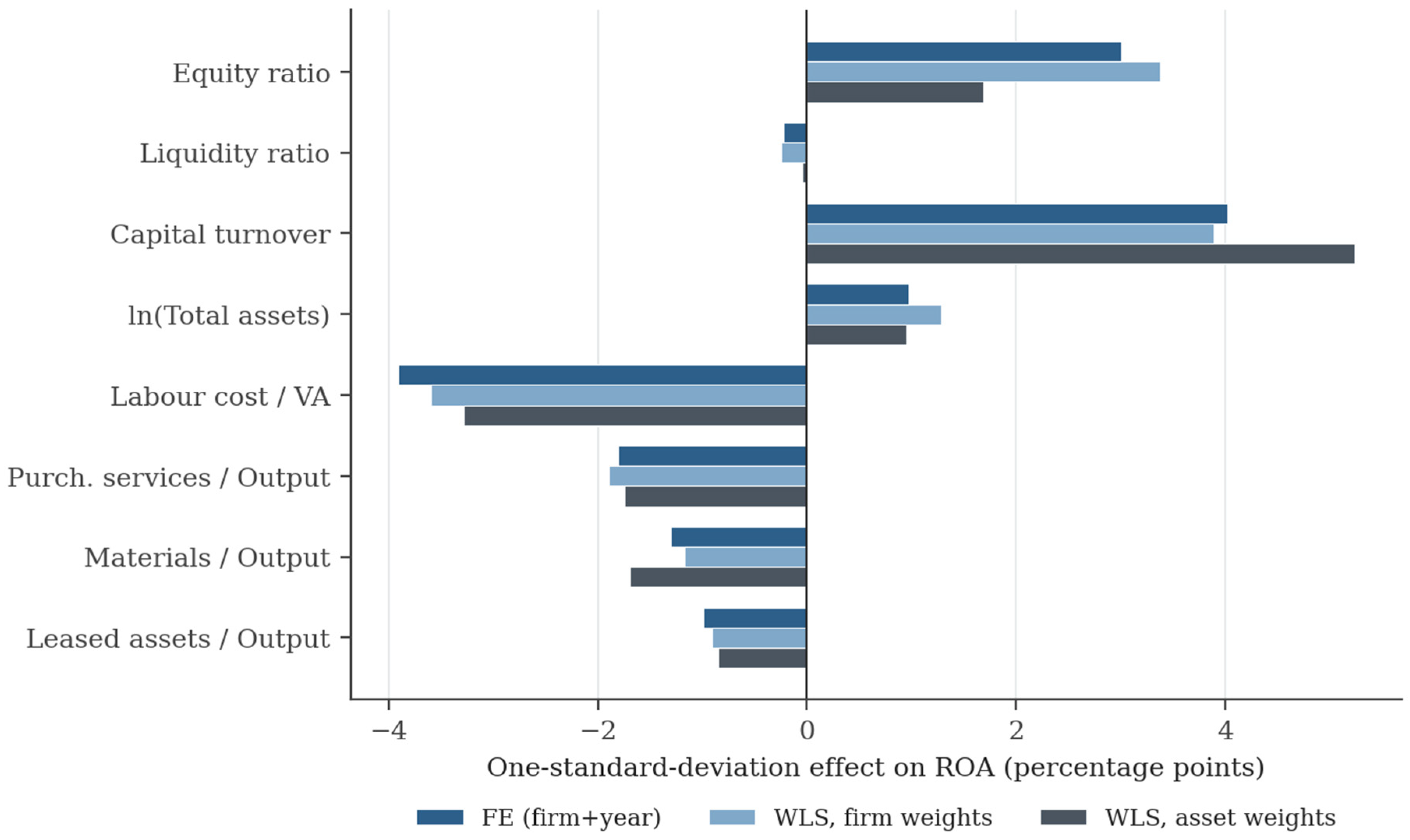
Under asset weights capital turnover gains and capitalisation loses roughly half its magnitude, while the operating cost shares are almost unmoved. A referee asking which weighting is correct is asking the wrong question, since the two answer different questions, and a paper about small-firm performance needs both. Figure A2 generalises the exercise from three specifications to nine, plotting for each regressor the full spread of standardised effects with the reference two-way estimate marked hollow.
Figure A2.
Coefficient stability across nine estimators.
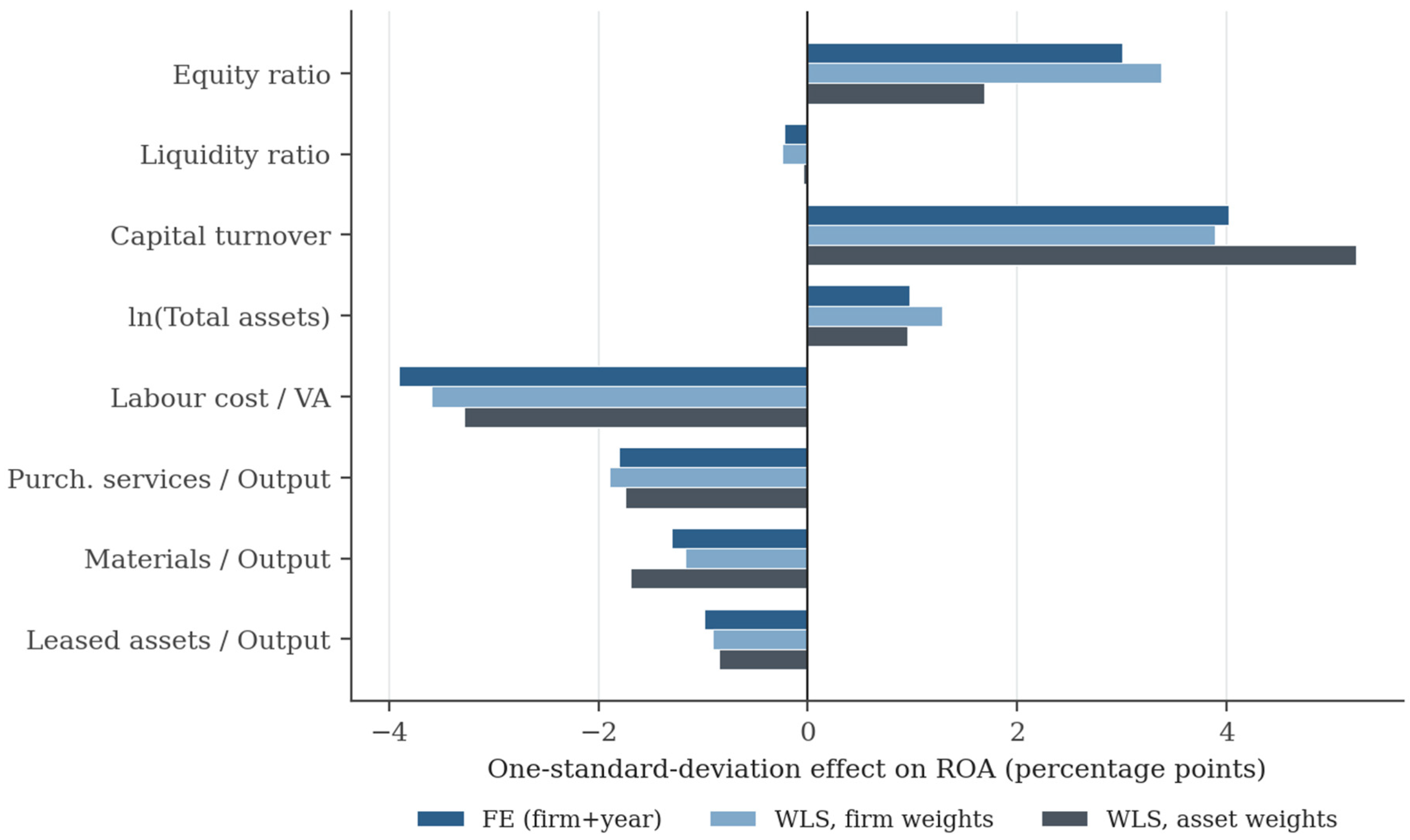
The two blocks separate cleanly. Among the financial variables the spread reaches 7.9 points of ROA for size and 5.0 for capitalisation, so the answer one obtains depends materially on the estimator chosen. Among the operating variables the spread is 3.5 points for the labour share, 2.3 for purchased services and 1.0 for leased assets, and in every case the whole spread is generated by the single lagged specification: dropping it collapses the labour share to a range of 0.4 points and materials to 0.2. The operating coefficients are therefore stable in a sense the financial coefficients are not, and this is the empirical basis for the reading advanced in Section 7.
The regime-specific estimates below are the input to the Wald tests reported in the text and plotted in Figure 5. Two patterns stand out beyond the tests themselves. Capital turnover carries a substantially larger coefficient among the two certified populations than among ordinary SMEs, consistent with turnover being the binding margin for firms that have not reached scale. And liquidity is insignificant or marginal in all three populations, which is worth stating explicitly because it is frequently included in this literature as a control and rarely reported as inert.
Table A3.
Separate estimation by regulatory regime. Two-way fixed effects.
| Regressor | Innovative start-ups | Innovative SMEs | Ordinary SMEs |
| Equity ratio (%) | 0.2317*** | 0.1589*** | 0.1626*** |
| (0.0126) | (0.0081) | (0.0074) | |
| Liquidity ratio | -0.2120* | -0.2353*** | -0.2130** |
| (0.1275) | (0.0898) | (0.0909) | |
| Capital turnover | 7.0189*** | 7.3493*** | 4.1749*** |
| (0.3735) | (0.3224) | (0.1530) | |
| ln(Total assets) | 3.4757*** | 0.8554*** | 0.4339*** |
| (0.3297) | (0.1934) | (0.1402) | |
| Labour cost / Value added (%) | -0.1311*** | -0.1170*** | -0.1632*** |
| (0.0054) | (0.0037) | (0.0050) | |
| Purchased services / Output (%) | -0.2357*** | -0.1902*** | -0.1493*** |
| (0.0160) | (0.0093) | (0.0084) | |
| Materials / Output (%) | -0.0926*** | -0.1499*** | -0.1137*** |
| (0.0285) | (0.0125) | (0.0082) | |
| Leased assets / Output (%) | -0.2608*** | -0.3029*** | -0.2653*** |
| (0.0334) | (0.0326) | (0.0297) | |
| Observations | 12,864 | 19,565 | 59,327 |
| Firms | 5,173 | 2,756 | 6,995 |
Note. Firm-clustered standard errors in parentheses. *** p<0.01, ** p<0.05, * p<0.10. Same specification and same observations asTable 3, partitioned by register membership.
The Wald statistics test equality of the full eight-element coefficient vector between each pair of populations, with variance equal to the sum of the two clustered covariance matrices. They are reported separately from Table A3 because a reader who inspects the three columns and sees overlapping standard errors on individual coefficients may conclude that the vectors are indistinguishable, which the joint test contradicts.
Table A4.
Wald tests of coefficient equality between regulatory regimes.
| Comparison | Wald χ² | d.f. | p |
| Innovative start-ups vs. innovative SMEs | 87.18 | 8 | < 0.0001 |
| Innovative start-ups vs. ordinary SMEs | 181.94 | 8 | < 0.0001 |
| Innovative SMEs vs. ordinary SMEs | 138.08 | 8 | < 0.0001 |
Note. Wald statistic on the difference between estimated vectors, with variance equal to the sum of the two clustered matrices. Eight degrees of freedom.
Appendix B. Instrumental Variables: Attempt and Diagnostics
The equity ratio is the regressor most exposed to simultaneity, and it is the one whose sign is unstable across the specifications of Figure 4. Five instrument sets were therefore tested within the two-way fixed-effects framework, with the equity ratio treated as endogenous and the remaining seven regressors as exogenous. Three come from inside the panel — the second lag of the equity ratio, the second and third lags jointly, and the second lag combined with an external instrument — and two are constructed: a leave-one-out province-year peer mean of the equity ratio, and net external equity injections, reconstructed as the change in net worth less the current year's profit, which is the one quantity that enters net worth without passing through current earnings.
Table B1.
Two-stage least squares with firm and year fixed effects. Coefficient on the equity ratio.
Table B1.
Two-stage least squares with firm and year fixed effects. Coefficient on the equity ratio.
| Instrument set | β (equity) | s.e. | First-stage F | Hansen J | p(J) |
| FE, no instruments (benchmark) | 0.1766*** | (0.0049) | — | — | — |
| (1) Equity ratio (t−2) | -0.2769*** | (0.0307) | 2,326.5 | — | — |
| (2) Equity ratio (t−2, t−3) | -0.2644*** | (0.0344) | 862.3 | 77.18 | 0.000 |
| (3) Province-year peer mean | -0.1227 | (0.2482) | 24.4 | — | — |
| (4) Net equity injections (t−1) | -0.2346*** | (0.0411) | 1,073.9 | — | — |
| (5) Injections (t−1) + equity (t−2) | -0.2579*** | (0.0225) | 2,224.0 | 1.02 | 0.313 |
Note. Firm-clustered standard errors. All specifications include firm and year fixed effects and the seven remaining regressors as exogenous controls. Hansen J is reported only for the overidentified specifications; sets (1), (3) and (4) are just identified and the restriction cannot be tested. Observations: 64,557 for (1) and (5), 53,386 for (2), 91,534 for (3), 64,656 for (4).
The table reports strength and validity in adjacent columns, which invites the conflation the two diagnostics are meant to prevent. Figure B1 separates them.
Figure B1.
Instrument strength and overidentification.
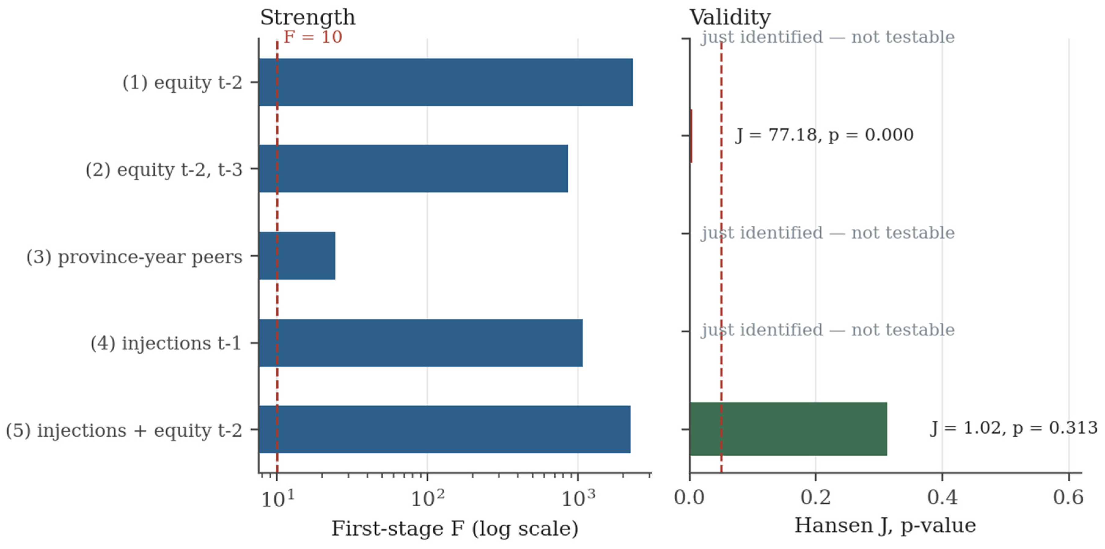
On the left, four of the five instrument sets clear the conventional weak-instrument threshold by two orders of magnitude and the province peer mean clears it by a factor of two. On the right, the specification using the second and third lags fails the overidentification test decisively; the specification combining injections with the second lag passes it. Strength and validity are independent properties, and these instruments have the first without reliably having the second. Figure B2 shows what the instruments do to the estimate that matters.
Figure B2.
The equity coefficient under five instrument sets.
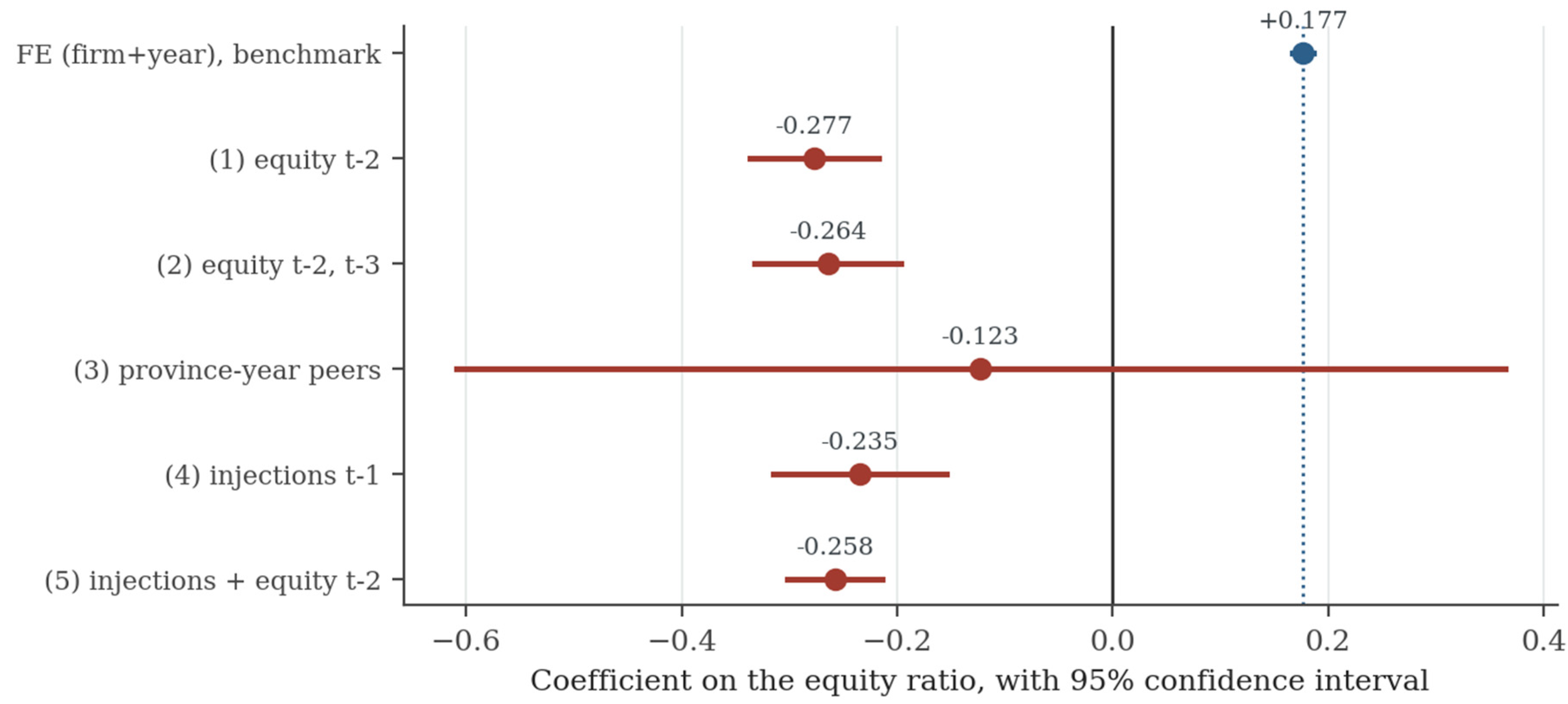
Every instrument set moves the coefficient from about +0.18 to between −0.12 and −0.28, and the four precisely estimated sets agree closely with one another while disagreeing sharply with the benchmark. That pattern is the opposite of reassuring. Instruments that identify the same parameter through genuinely different exclusion restrictions should agree with one another only if all the restrictions hold; here the internal instruments share a single failure mode, which is why they agree, and the one instrument with an independent restriction is too weak to arbitrate.
Why the Instruments Fail
First, overidentification is rejected where it can be tested. Specification (2) returns a Hansen J of 77.18 with p below 0.001. Specification (5) does not reject at 1.02, but its point estimate of −0.258 lies inside the range spanned by the specifications that do reject, so passing the test does not distinguish it substantively; it is a weaker test on a smaller set of restrictions, not independent evidence of validity.
Second, the mechanism of failure is identifiable rather than merely suspected. The autoregressive coefficient of ROA is 0.271, so profitability at t is substantially predicted by profitability at t−2. Since the equity ratio at t−2 mechanically embeds the profit of t−2, lagged capitalisation is correlated with the current error through persistence alone. This is a direct violation of the exclusion restriction rather than a subtle one, and no lag length escapes it while profitability remains persistent: lengthening the lag weakens the first stage without breaking the chain that runs from past profit to present profit.
Third, the one instrument whose exclusion restriction is defensible on economic grounds is too weakly related to the endogenous regressor to be usable. Net external equity injections enter net worth without passing through current profit, which is exactly what the restriction requires, but their within-firm correlation with the equity ratio is 0.103. Because the asymptotic bias of two-stage least squares stands to that of least squares roughly as the correlation between instrument and error stands to the correlation between instrument and regressor, a correlation of 0.103 amplifies any violation of exclusion by a factor of about ten. The first-stage F of 1,074 reflects the size of the sample rather than instrument strength in the sense that matters here, which is a distinction the F statistic is not designed to make.
Table B2.
Assessment of each instrument set against the two requirements.
| Instrument set | Exclusion restriction rests on | Strength | Validity | Usable |
| (1) Equity (t−2) | Absence of profit persistence | Very strong | Violated by construction | No |
| (2) Equity (t−2, t−3) | Absence of profit persistence | Very strong | Rejected, J = 77.18 | No |
| (3) Province-year peers | No local demand shocks | Weak in substance | Not testable | No |
| (4) Equity injections (t−1) | Injections independent of current profit | Nominal F only | Defensible | No |
| (5) Injections + equity (t−2) | Both of the above jointly | Very strong | Not rejected, J = 1.02 | Not decisive |
Note. Strength is assessed on the within-firm correlation between instrument and regressor rather than on the first-stage F alone, since with more than sixty thousand observations the F statistic is large for correlations far too low to control bias amplification.
Placement of the Instrumental-Variable Results
Whether these results belong in the body of the paper or in an appendix is a judgement, and the case for each is worth stating. The argument for the body is that the instrumented estimates reverse the sign of the leading coefficient, and a result of that magnitude ordinarily belongs where the reader will see it. The argument for the appendix is that the instruments do not identify the parameter: two of the five fail a test they can be given, a third is weak in substance, and the mechanism of failure is common to all the internal instruments. Estimates from a rejected identification strategy reported alongside estimates from an accepted one invite the reader to average them, which would be the wrong operation.
The compromise adopted here places the summary in the body and the machinery in the appendix. Figure 4 in Section 4 carries every instrumental-variable point estimate, so the reader sees the reversal and its magnitude without being asked to accept it; one paragraph states that the instruments fail and why; and the tables, diagnostics and the reasoning behind the verdict sit here. What is not done, and what the literature surveyed in Section 2 does frequently, is to report a single instrumented column as the paper's preferred specification on the strength of a first-stage F alone. On this sample that column exists — specification (5), which passes its overidentification test with a coefficient of −0.258 — and reporting it as the answer would be the most misleading single choice available.
The wider conclusion is negative and is stated as such: these data contain no valid instrument for financial structure. The feature that makes the dynamic specification necessary, the persistence of profitability at 0.271, is the same feature that destroys the internal instruments, and the external instrument that survives the argument does not survive the arithmetic of bias amplification. Identification of the capitalisation coefficient would require exogenous variation in financial structure — a regulatory threshold, a tax change, a lending shock differentially binding across otherwise similar firms — and no such variation is present in an accounting panel of this construction.
Appendix C. Clustering: Full Validity Battery and Within-Cluster Estimates
Reading down the silhouette column of Table A1 shows why no single index can decide the question. Silhouette falls monotonically in k for every partitional method, so on that criterion k = 2 always wins, and Calinski–Harabasz behaves the same way; partition R² and the Dunn index move in the opposite direction. The two density-based configurations attain high silhouette while assigning between four and thirty-three per cent of firms to noise, and they are excluded on that ground rather than on their index values. The table is reported in full, including the configurations that were rejected, because the argument for the composite ranking rests on the disagreement between the indices and cannot be assessed from the winning row alone.
Table C1.
Validity battery across algorithms and numbers of clusters.
| Algorithm | k | Silh. | CH | DB | Dunn | MaxDiam | MinSep | γ | Entropy | HHI | R² | BIC | Min % |
| k-means | 2 | 0.210 | 3472 | 1.851 | 0.0186 | 25.66 | 0.478 | 0.305 | 0.668 | 0.525 | 0.189 | — | 38.8 |
| Ward | 2 | 0.167 | 2731 | 2.110 | 0.0175 | 25.66 | 0.449 | 0.232 | 0.690 | 0.503 | 0.155 | — | 46.2 |
| Gaussian mix. | 2 | 0.115 | 1631 | 2.716 | 0.0135 | 25.66 | 0.345 | 0.154 | 0.683 | 0.510 | 0.099 | 316,325 | 43.0 |
| Fuzzy c-means | 2 | 0.198 | 3377 | 1.902 | 0.0134 | 25.66 | 0.344 | 0.281 | 0.690 | 0.504 | 0.184 | — | 45.7 |
| k-means | 3 | 0.172 | 2880 | 1.836 | 0.0161 | 21.65 | 0.348 | 0.281 | 1.091 | 0.338 | 0.278 | — | 28.4 |
| Ward | 3 | 0.146 | 2149 | 2.145 | 0.0180 | 21.58 | 0.389 | 0.285 | 1.043 | 0.369 | 0.224 | — | 19.6 |
| Gaussian mix. | 3 | 0.120 | 1460 | 3.324 | 0.0122 | 25.66 | 0.314 | 0.243 | 1.089 | 0.340 | 0.164 | 282,504 | 27.9 |
| Fuzzy c-means | 3 | 0.146 | 2503 | 2.217 | 0.0147 | 23.15 | 0.340 | 0.277 | 1.088 | 0.340 | 0.251 | — | 26.7 |
| k-means | 4 | 0.172 | 2601 | 1.784 | 0.0159 | 21.55 | 0.342 | 0.316 | 1.347 | 0.269 | 0.343 | — | 14.9 |
| Ward | 4 | 0.154 | 1965 | 1.804 | 0.0180 | 21.58 | 0.389 | 0.313 | 1.130 | 0.358 | 0.283 | — | 3.2 |
| Gaussian mix. | 4 | 0.077 | 1227 | 3.300 | 0.0097 | 25.66 | 0.249 | 0.272 | 1.331 | 0.275 | 0.198 | 273,297 | 13.2 |
| Fuzzy c-means | 4 | 0.108 | 1909 | 2.841 | 0.0118 | 22.44 | 0.264 | 0.271 | 1.285 | 0.292 | 0.277 | — | 8.3 |
| k-means | 5 | 0.177 | 2518 | 1.654 | 0.0162 | 21.55 | 0.348 | 0.366 | 1.460 | 0.247 | 0.403 | — | 3.5 |
| Ward | 5 | 0.148 | 1935 | 1.921 | 0.0180 | 21.58 | 0.389 | 0.344 | 1.439 | 0.257 | 0.342 | — | 3.2 |
| Gaussian mix. | 5 | 0.065 | 1284 | 3.335 | 0.0101 | 25.66 | 0.260 | 0.256 | 1.562 | 0.217 | 0.256 | 262,697 | 9.9 |
| Fuzzy c-means | 5 | 0.077 | 1557 | 5.071 | 0.0118 | 22.01 | 0.260 | 0.265 | 1.441 | 0.258 | 0.294 | — | 5.1 |
| k-means | 6 | 0.179 | 2453 | 1.533 | 0.0162 | 21.55 | 0.348 | 0.403 | 1.572 | 0.229 | 0.451 | — | 3.4 |
| Ward | 6 | 0.141 | 1855 | 1.691 | 0.0180 | 21.58 | 0.389 | 0.358 | 1.553 | 0.243 | 0.383 | — | 3.2 |
| Gaussian mix. | 6 | 0.059 | 1101 | 3.129 | 0.0102 | 25.54 | 0.260 | 0.246 | 1.749 | 0.180 | 0.269 | 257,268 | 8.2 |
| Fuzzy c-means | 6 | 0.053 | 1225 | 10.733 | 0.0118 | 22.01 | 0.260 | 0.262 | 1.430 | 0.264 | 0.291 | — | 0.9 |
| k-means | 7 | 0.169 | 2357 | 1.508 | 0.0159 | 20.63 | 0.329 | 0.393 | 1.758 | 0.190 | 0.487 | — | 3.1 |
| Ward | 7 | 0.086 | 1716 | 1.799 | 0.0150 | 20.74 | 0.311 | 0.304 | 1.777 | 0.189 | 0.408 | — | 3.2 |
| Gaussian mix. | 7 | 0.050 | 994 | 3.052 | 0.0063 | 25.66 | 0.163 | 0.258 | 1.868 | 0.165 | 0.286 | 241,245 | 7.9 |
| Fuzzy c-means | 7 | 0.076 | 1065 | 8.066 | 0.0180 | 21.59 | 0.389 | 0.263 | 1.521 | 0.239 | 0.300 | — | 0.2 |
| DBSCAN (ε=0.6) | 5 | -0.176 | 269 | 1.409 | 0.1504 | 3.98 | 0.598 | -0.078 | 0.725 | 0.608 | 0.083 | — | 1.1 |
| DBSCAN (ε=0.8) | 4 | -0.075 | 270 | 2.092 | 0.1192 | 7.04 | 0.840 | 0.065 | 0.096 | 0.969 | 0.067 | — | 0.3 |
| RF proximity | 2 | 0.202 | 911 | 1.957 | 0.0167 | 23.82 | 0.398 | 0.299 | 0.600 | 0.591 | 0.154 | — | 28.7 |
| RF proximity | 3 | 0.161 | 652 | 2.263 | 0.0160 | 23.82 | 0.382 | 0.345 | 0.942 | 0.437 | 0.207 | — | 13.3 |
| RF proximity | 4 | -0.043 | 439 | 2.649 | 0.0160 | 23.82 | 0.382 | 0.334 | 0.990 | 0.426 | 0.209 | — | 0.9 |
Note. γ is the Pearson gamma between pairwise distances and the co-membership indicator. Entropy and the Herfindahl–Hirschman index measure balance across clusters. BIC is defined only for the Gaussian mixture. Min % is the share of firms in the smallest cluster; for the density-based rows it excludes the firms assigned to noise. Indices requiring pairwise distances are computed on a random subsample of 5,000 firms. The shaded row is the selected configuration.
Figure A1 plots the four indices that disagree most sharply, restricted to the partitional families for legibility. Taken together the four panels make the selection problem visible: silhouette and Calinski–Harabasz decline in k while partition R² rises, and the Dunn index is nearly flat for k-means across the whole range.
Figure C1.
Validity indices across algorithms and number of clusters.
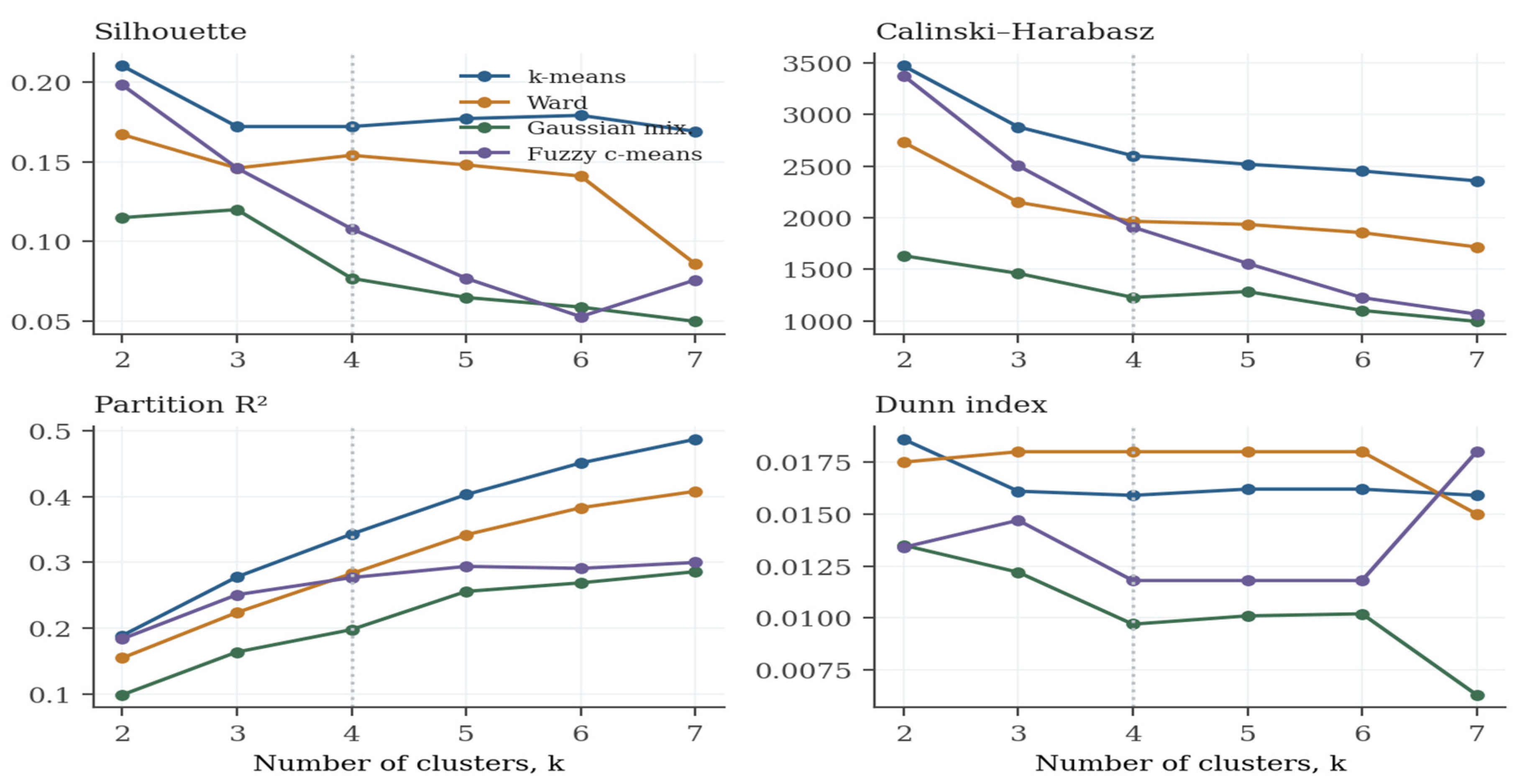
Density-based and random-forest proximity configurations are omitted from the panels and reported in Table A1. The dotted vertical line marks the selected k. Nothing in any single panel identifies it: k = 4 is the point at which k-means leads on partition R² among the solutions that remain balanced, and the composite ranking below is what makes that consideration operative.
Figure C2.
Composite ranking of the retained configurations.
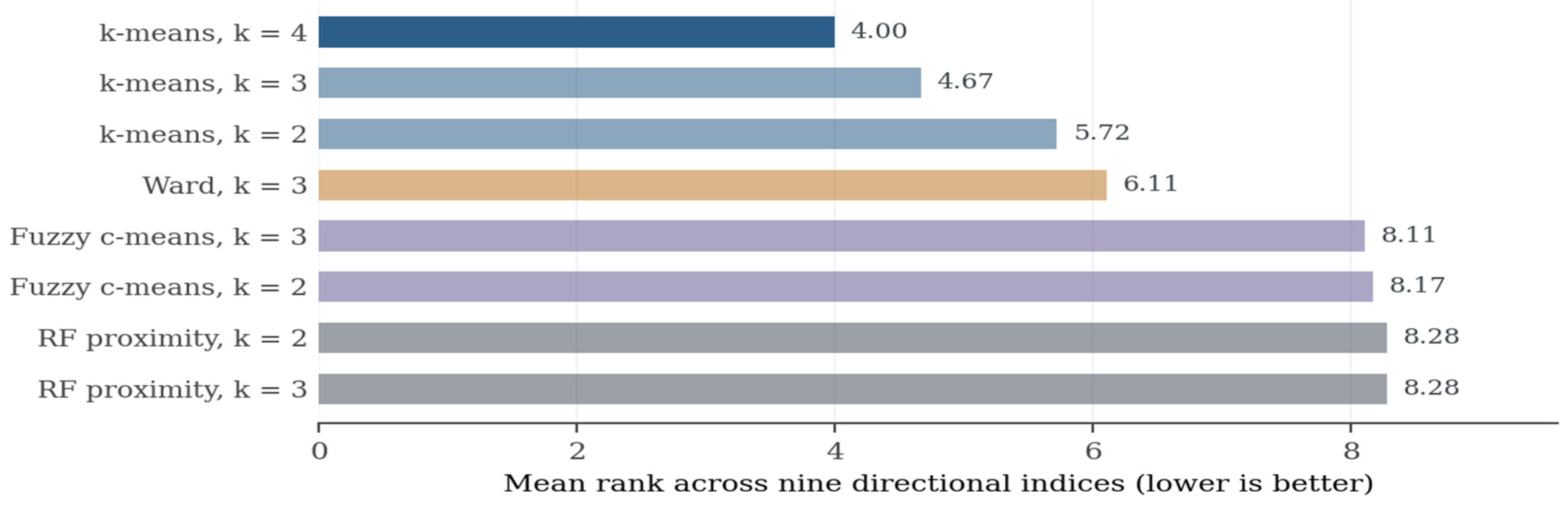
The composite ranking separates k = 4 from its nearest rival by a narrow margin, and the two leading configurations were therefore both examined in full. At k = 3 the labour-intensive and materials-intensive groups are unchanged and the micro-service and capitalised groups merge; the coefficient pattern of Table A5 survives, with capital turnover still ranging by a factor of three across groups and the labour share still invariant. Fuzzy c-means at k = 2 and k = 3 rank immediately behind k-means, which is reassuring rather than redundant, since the same structure is reached by a procedure that does not impose hard assignment.
Table C2.
Composite ranking (mean rank across nine directional indices; lower is better).
| Algorithm | k | Composite rank |
| k-means | 4 | 4.00 |
| k-means | 3 | 4.67 |
| k-means | 2 | 5.72 |
| Ward | 3 | 6.11 |
| Fuzzy c-means | 3 | 8.11 |
| Fuzzy c-means | 2 | 8.17 |
| RF proximity | 2 | 8.28 |
| RF proximity | 3 | 8.28 |
Note. Configurations with a smallest cluster below five per cent of firms are excluded, as are density-based solutions classifying more than five per cent of firms as noise. Nine of the eleven criteria are directional and enter the mean rank; maximum diameter and BIC are reported in Table A1 but not ranked, the first because it is bounded by the sample and the second because it is defined for one family only.
Table A3 reports the medians, interpretable in the original units, alongside the standardised means that show each variable's contribution to the separation. The two columns tell different stories about the financial variables. In medians, Cluster 3 is four times as capitalised as Cluster 0, 70.1 against 17.3, and its liquidity ratio is three times as high; in standardised terms both variables are flat across the other three clusters, so their large ranges are generated by a single group. The labour share moves across all four groups, from +0.71 to −0.80, and purchased services from +0.92 to −0.72.
Table C3.
Cluster profiles, medians and standardised means.
| Variable | C0 med. | C1 med. | C2 med. | C3 med. | C0 std. | C1 std. | C2 std. | C3 std. |
| ROA (%) | 3.03 | 4.72 | 7.36 | 10.23 | -0.43 | -0.06 | 0.30 | 0.60 |
| Equity ratio (%) | 17.29 | 33.22 | 34.71 | 70.10 | -0.60 | 0.01 | 0.01 | 1.33 |
| Liquidity ratio | 1.22 | 1.08 | 1.31 | 3.70 | -0.27 | -0.39 | -0.27 | 1.76 |
| Capital turnover | 1.23 | 1.03 | 0.69 | 0.59 | 0.38 | 0.11 | -0.31 | -0.56 |
| ln(Total assets) | 7.58 | 9.75 | 4.79 | 5.60 | 0.16 | 0.93 | -0.94 | -0.53 |
| Labour cost / VA (%) | 89.63 | 67.55 | 0.63 | 35.23 | 0.71 | 0.06 | -0.80 | -0.44 |
| Purch. services / Output (%) | 29.94 | 18.88 | 57.35 | 34.94 | -0.13 | -0.72 | 0.92 | 0.08 |
| Materials / Output (%) | 3.04 | 47.43 | 0.81 | 0.82 | -0.42 | 1.29 | -0.54 | -0.50 |
| Leased assets / Output (%) | 3.69 | 1.95 | 0.68 | 1.15 | 0.39 | -0.20 | -0.25 | -0.13 |
| Firms | 5,067 | 4,023 | 3,615 | 2,224 | ||||
| Share of firms (%) | 33.9 | 26.9 | 24.2 | 14.9 |
Note. Medians are of firm-level decade medians in original units. Standardised means are computed on the standardised variables used by the algorithm.
The contingency of the partition with regulatory status is reported below as row percentages, so that each row is the distribution of one register population across the four archetypes. Regulatory status enters no stage of the clustering procedure.
Table C4.
Contingency of partition with regulatory status (row percentages).
| Regulatory population | C0 labour | C1 materials | C2 micro service | C3 capitalised |
| Innovative start-ups | 16.7 | 6.1 | 53.1 | 24.2 |
| Innovative SMEs | 35.7 | 15.5 | 27.4 | 21.3 |
| Ordinary SMEs | 46.0 | 46.9 | 1.6 | 5.5 |
Note. χ²(6) = 6,821.9, p < 0.0001, Cramér's V = 0.4780. Rows sum to 100.
The full within-cluster estimates follow, plotted first because the coefficients occupy two very different scales: turnover and size are an order of magnitude larger than the cost shares and cannot be read on a common axis. Three features deserve attention beyond the dispersion discussed in Section 5. Liquidity is insignificant in three of the four groups, confirming from an independent direction the inertness already visible in Section 4. Materials are insignificant in the capitalised cluster, where the median materials share is 0.82 per cent of output and the variable has almost no variation to exploit — an absence of data rather than an absence of effect. And the labour share is the only coefficient whose confidence intervals overlap across all four groups.
Figure C3.
Equation coefficients re-estimated within each cluster.
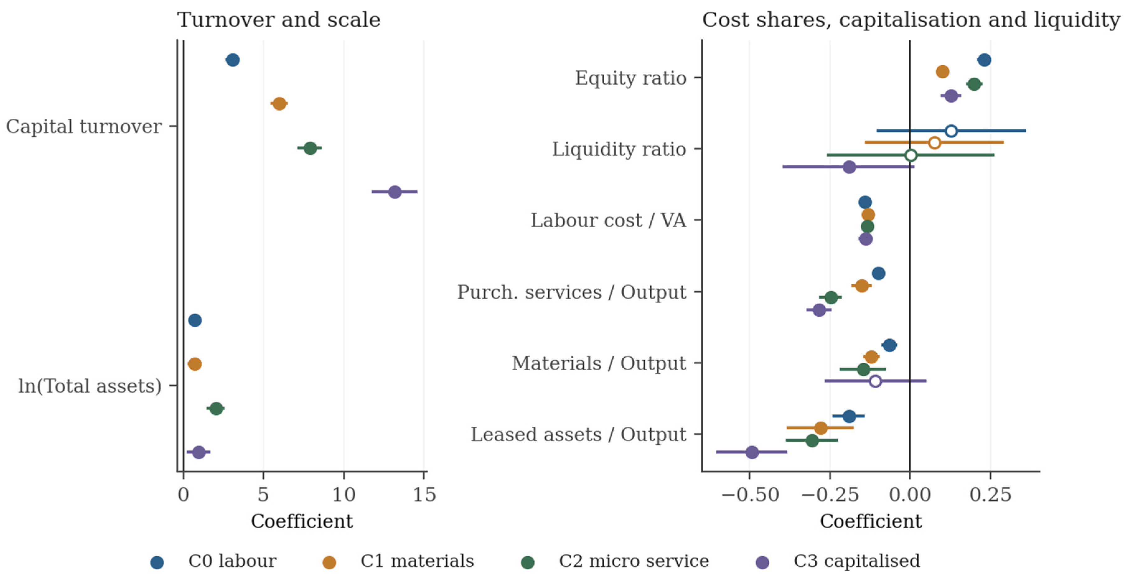
Hollow markers denote coefficients not significant at the ten per cent level. The intervals are ninety-five per cent and firm-clustered. Table A5 gives the same estimates with standard errors and fit statistics.
Table C5.
Equation re-estimated within each cluster. Dependent variable: ROA (%).
| Regressor | C0 labour | C1 materials | C2 micro service | C3 capitalised |
| Equity ratio (%) | 0.2314*** | 0.1015*** | 0.2002*** | 0.1280*** |
| (0.0091) | (0.0069) | (0.0104) | (0.0136) | |
| Liquidity ratio | 0.1279 | 0.0756 | 0.0015 | -0.1909* |
| (0.1163) | (0.1081) | (0.1311) | (0.1025) | |
| Capital turnover | 3.0860*** | 5.9623*** | 7.8726*** | 13.1552*** |
| (0.1742) | (0.2216) | (0.3498) | (0.6774) | |
| ln(Total assets) | 0.7229*** | 0.6971*** | 2.0210*** | 0.9727*** |
| (0.1583) | (0.1736) | (0.2450) | (0.3274) | |
| Labour cost / Value added (%) | -0.1403*** | -0.1317*** | -0.1347*** | -0.1383*** |
| (0.0038) | (0.0047) | (0.0061) | (0.0084) | |
| Purchased services / Output (%) | -0.0980*** | -0.1510*** | -0.2475*** | -0.2852*** |
| (0.0075) | (0.0139) | (0.0155) | (0.0176) | |
| Materials / Output (%) | -0.0646*** | -0.1205*** | -0.1466*** | -0.1081 |
| (0.0105) | (0.0104) | (0.0347) | (0.0789) | |
| Leased assets / Output (%) | -0.1909*** | -0.2800*** | -0.3051*** | -0.4937*** |
| (0.0234) | (0.0505) | (0.0390) | (0.0545) | |
| Observations | 34,377 | 34,632 | 12,804 | 10,062 |
| Firms | 5,060 | 4,019 | 3,612 | 2,223 |
| Within R² | 0.4293 | 0.4955 | 0.4420 | 0.4759 |
Note. Two-way fixed effects, firm-clustered standard errors in parentheses. *** p<0.01, ** p<0.05, * p<0.10. Firm counts fall marginally below those of Table A3 because a small number of firms contribute no usable within variation once the equation is estimated inside the group.
The Wald statistics test equality of the full eight-element coefficient vector for each pair of clusters, with variance equal to the sum of the two clustered covariance matrices. They are reported for completeness rather than as the decisive evidence: on samples of this size rejection is close to automatic, and the informative quantity is the magnitude of the differences plotted in Figure 8, not the p-value attached to them.
Table C6.
Pairwise Wald tests of coefficient equality across clusters.
| Comparison | χ² | d.f. | p |
| Cluster 0 vs. Cluster 1 | 264.42 | 8 | < 0.0001 |
| Cluster 0 vs. Cluster 2 | 262.68 | 8 | < 0.0001 |
| Cluster 0 vs. Cluster 3 | 374.34 | 8 | < 0.0001 |
| Cluster 1 vs. Cluster 2 | 125.42 | 8 | < 0.0001 |
| Cluster 1 vs. Cluster 3 | 153.27 | 8 | < 0.0001 |
| Cluster 2 vs. Cluster 3 | 84.45 | 8 | < 0.0001 |
Note. Eight degrees of freedom. The smallest statistic, 84.45, is between the micro-service and capitalised clusters, which are also the two groups the three-cluster solution merges.
Appendix D. Machine-Learning Regression, Full Results
The algorithm comparison is reported on raw levels, as such comparisons are conventionally presented; the like-for-like within-transformed figures of Section 6 are those comparable with the panel estimates. Two columns beyond the headline deserve attention. The cross-fold standard deviation separates stable learners from unstable ones: the leading methods sit between 0.0066 and 0.0082 while AdaBoost reaches 0.1250, meaning its accuracy depends heavily on which firms fall into the test partition. And the timing column matters for replication, since histogram gradient boosting attains the best accuracy in 3.3 seconds against 120.5 for the random forest.
Table D1.
Algorithm comparison, raw levels.
| Model | R² (out of sample) | SD across folds | RMSE | MAE | Seconds |
| Histogram gradient boosting | 0.7978 | 0.0070 | 5.932 | 3.476 | 3.3 |
| Neural network (MLP) | 0.7875 | 0.0082 | 6.082 | 3.613 | 52.5 |
| Random forest | 0.7786 | 0.0078 | 6.209 | 3.646 | 120.5 |
| Extra trees | 0.7650 | 0.0076 | 6.397 | 3.803 | 19.4 |
| Gradient boosting | 0.7195 | 0.0072 | 6.989 | 4.299 | 95.7 |
| k-nearest neighbours | 0.6945 | 0.0069 | 7.293 | 4.472 | 10.7 |
| Decision tree | 0.6436 | 0.0066 | 7.877 | 4.893 | 2.3 |
| Lasso | 0.4730 | 0.0112 | 9.578 | 6.210 | 0.2 |
| Ridge | 0.4730 | 0.0112 | 9.578 | 6.212 | 0.2 |
| Linear regression | 0.4730 | 0.0112 | 9.578 | 6.212 | 0.2 |
| Elastic net | 0.4730 | 0.0111 | 9.578 | 6.208 | 0.2 |
| Linear SVM | 0.4551 | 0.0108 | 9.740 | 6.065 | 1.8 |
| AdaBoost | 0.2060 | 0.1250 | 11.714 | 8.510 | 25.7 |
Note. Dependent variable ROA (%), same eight regressors and same 91,756 observations as the panel estimates. Five-fold cross-validation grouped by firm. The shaded row is the algorithm carried forward.
Figure D1.
Out-of-sample accuracy by algorithm, and accuracy against fitting time.
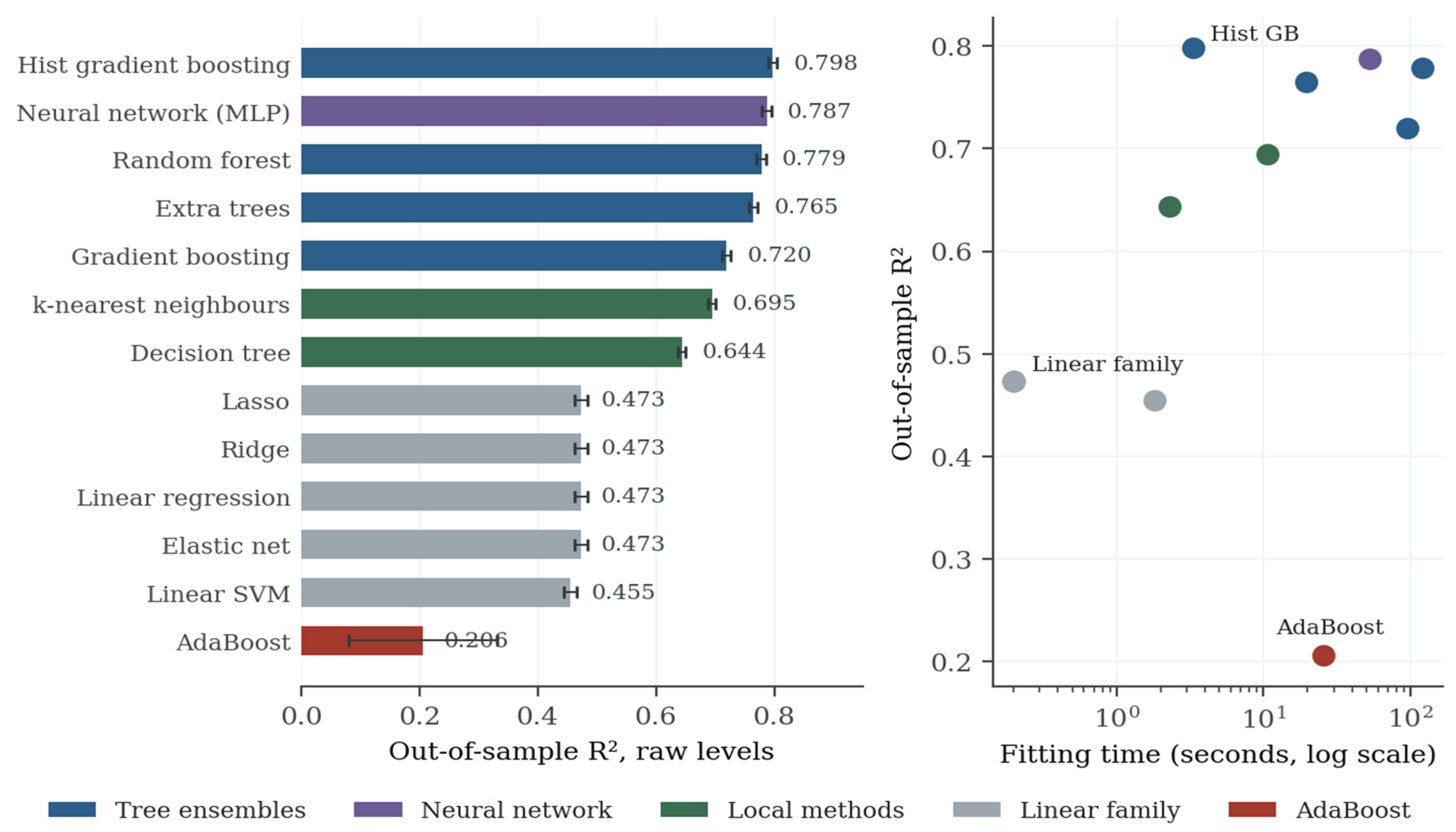
Three bands emerge rather than a continuum, and they correspond to what each family can represent: thresholds and interactions, smooth local structure, and additive linearity. The right-hand panel adds the dimension a ranking hides. Accuracy is not bought with computation — the selected algorithm is thirty-six times faster than the random forest it outperforms — and the linear family is separated from the ensembles by a difference in representational capacity rather than in effort. AdaBoost is the one clear failure in the battery, its exponential reweighting chasing the tails of a heavy-tailed target; its failure characterises the distribution rather than the specification, and it is retained in the table for that reason.
The learning curve settles whether the remaining gap is an artefact of sample size. The gradient-boosting test score rises little over the final two thirds of the data while its training score falls towards it, which is the signature of a model that has stopped memorising rather than one starved of observations. The linear model is flat almost from the start.
Figure D2.
Learning curves, firm-demeaned data.
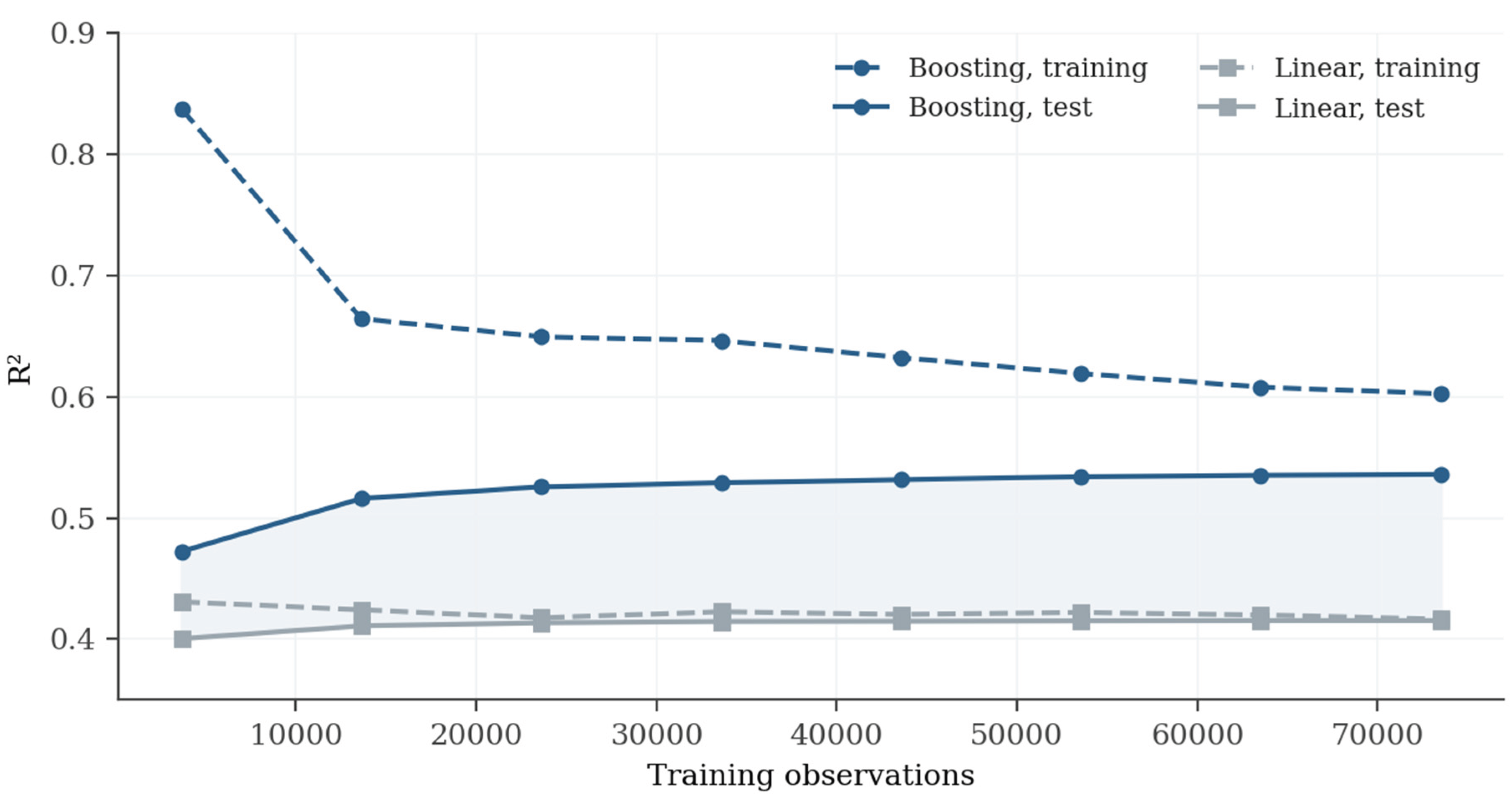
Table D2.
Learning curve values.
| Training observations | Linear, train | Linear, test | Boosting, train | Boosting, test |
| 3,675 | 0.4309 | 0.4005 | 0.8372 | 0.4724 |
| 13,650 | 0.4243 | 0.4110 | 0.6642 | 0.5161 |
| 23,624 | 0.4177 | 0.4136 | 0.6494 | 0.5257 |
| 33,600 | 0.4227 | 0.4146 | 0.6463 | 0.5290 |
| 43,575 | 0.4206 | 0.4148 | 0.6322 | 0.5316 |
| 53,550 | 0.4222 | 0.4151 | 0.6191 | 0.5340 |
| 63,525 | 0.4200 | 0.4153 | 0.6079 | 0.5353 |
| 73,500 | 0.4167 | 0.4153 | 0.6025 | 0.5360 |
Note. The shaded band in Figure A2 is the distance between the two test curves, which is the quantitySection 6 discusses. More data will not close it: the linear test score moves by 0.015 across a twenty-fold increase in training observations.
Interaction strength is measured by the Friedman H-statistic, which reports the share of the joint partial-dependence variation attributable to interaction rather than to the two separate effects. The strongest pair is the equity ratio with capital turnover at 0.042 — real but second-order. A purely additive surface would return zero throughout.
Figure D3.
Interaction strength by pair.
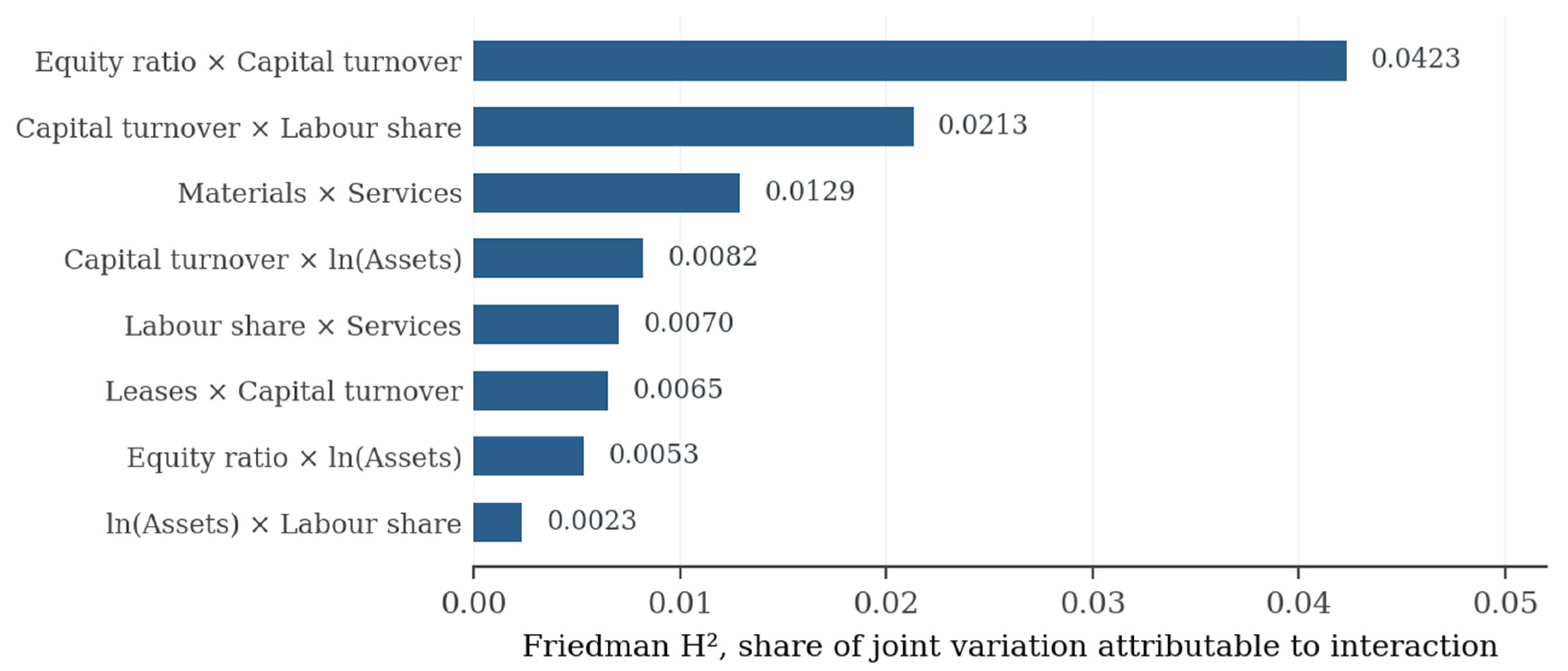
Table D3.
Friedman H-statistic by pair.
| Pair | H² |
| Equity ratio × Capital turnover | 0.0423 |
| Capital turnover × Labour share | 0.0213 |
| Materials / Output × Services / Output | 0.0129 |
| Capital turnover × ln(Total assets) | 0.0082 |
| Labour share × Services / Output | 0.0070 |
| Leases / Output × Capital turnover | 0.0065 |
| Equity ratio × ln(Total assets) | 0.0053 |
| ln(Total assets) × Labour share | 0.0023 |
Note. Computed on a 3,000-observation subsample of the held-out fold. The result corroborates the parametric exercise from the other direction: interactions recovered 16.7 per cent of the gap against 13.7 for squared terms alone, so neither dominates and both leave four fifths unexplained.
Permutation importance is computed on held-out data, so it measures contribution to genuine prediction rather than in-sample fit. The four lowest predictors together account for 6.9 per cent of predictive content, which means the equation could be reduced to four regressors with modest predictive loss — though not without losing controls the panel specification requires for reasons that have nothing to do with prediction.
Table D4.
Permutation importance, firm-demeaned data.
| Predictor | Drop in R² | SD | Share of total (%) |
| Labour share | 0.6247 | 0.0132 | 63.5 |
| Capital turnover | 0.1309 | 0.0034 | 13.3 |
| Services / Output | 0.0946 | 0.0017 | 9.6 |
| Equity ratio | 0.0642 | 0.0010 | 6.5 |
| Materials / Output | 0.0257 | 0.0018 | 2.6 |
| Leases / Output | 0.0187 | 0.0010 | 1.9 |
| ln(Total assets) | 0.0137 | 0.0007 | 1.4 |
| Liquidity ratio | 0.0110 | 0.0011 | 1.1 |
Note. Twenty permutations per predictor on the held-out fold. Shares are of the summed drop across the eight predictors.
Accuracy by subgroup is reported against both partitions used in the paper, the regulatory one of Section 4 and the estimated one of Section 5. The gap between linear and non-linear fits is widest in the materials-intensive cluster and narrowest in the micro-service one, where the linear form is nearly adequate. The absolute levels matter as much as the gaps: between 38 and 48 per cent of within-firm variation is linearly predictable in every subgroup, a more even picture than the pooled figures suggest.
Figure D4.
Out-of-sample accuracy by subgroup, firm-demeaned data.
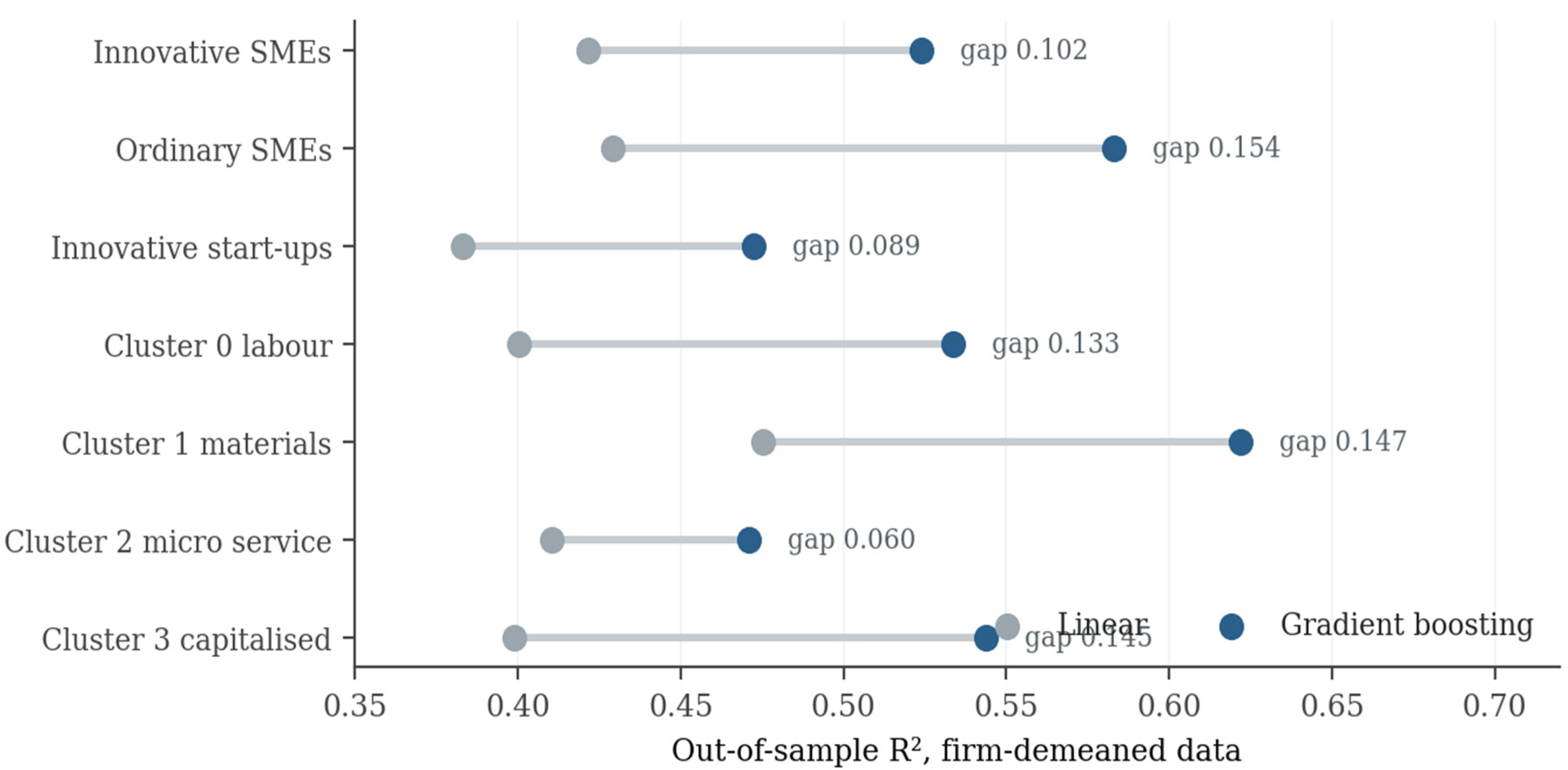
Table D5.
Out-of-sample accuracy by subgroup, firm-demeaned data.
| Subgroup | Observations | Linear R² | Boosting R² | Gap |
| Innovative SMEs | 19,576 | 0.4215 | 0.5238 | 0.1023 |
| Ordinary SMEs | 59,435 | 0.4291 | 0.5829 | 0.1537 |
| Innovative start-ups | 12,864 | 0.3830 | 0.4723 | 0.0893 |
| Cluster 0 labour | 34,377 | 0.4004 | 0.5336 | 0.1331 |
| Cluster 1 materials | 34,632 | 0.4752 | 0.6218 | 0.1466 |
| Cluster 2 micro service | 12,804 | 0.4106 | 0.4710 | 0.0604 |
| Cluster 3 capitalised | 10,062 | 0.3988 | 0.5436 | 0.1447 |
Note. Each subgroup is fitted and evaluated separately with the same five-fold grouped cross-validation. Observation counts for the regulatory populations differ marginally fromTable 2 because the subgroup fits require a complete lag-free record.
Finally the decile calibration underlying Figure 12. Reading down the two bias columns shows that both models are well calibrated in the middle six deciles and that essentially all of the difference between them arises in the two deciles at each end.
Table D6.
Prediction bias by decile of realised profitability.
| Decile | Actual mean | Linear mean | Boosting mean | Linear bias | Boosting bias |
| 1 | -16.46 | -7.86 | -9.02 | +8.60 | +7.43 |
| 2 | -5.70 | -2.73 | -4.28 | +2.97 | +1.42 |
| 3 | -3.09 | -1.42 | -2.63 | +1.66 | +0.45 |
| 4 | -1.55 | -0.74 | -1.57 | +0.82 | -0.02 |
| 5 | -0.48 | -0.22 | -0.59 | +0.26 | -0.11 |
| 6 | 0.26 | 0.23 | 0.22 | -0.04 | -0.04 |
| 7 | 1.34 | 1.04 | 1.57 | -0.30 | +0.22 |
| 8 | 3.04 | 1.90 | 2.76 | -1.14 | -0.28 |
| 9 | 6.04 | 3.22 | 4.59 | -2.82 | -1.45 |
| 10 | 16.59 | 6.58 | 8.88 | -10.01 | -7.71 |
Note. Firm-demeaned ROA on the held-out fold. Bias is predicted minus actual, so positive values indicate over-prediction. Deciles are of realised profitability, so the first and last rows are the observations on which any specification of this equation performs worst.
References
- Abbate, S.; Centobelli, P.; Cerchione, R. The digital and sustainable transition of the agri-food sector. Technol. Forecast. Soc. Change 2023, 187, 122222. [Google Scholar] [CrossRef]
- Abdalla, Y. A.; Ahmed, I. E.; Jafeel, A. Y. Family businesses in the GCC: What drives their capital structure? Borsa Istanb. Rev. 2025, 25(6), 1128–1136. [Google Scholar] [CrossRef]
- Abdeljawad, I.; Farhood, H. The trade-off behavior of capital structure in firms within politically unstable emerging countries. Manag. Sustain. 2025. [Google Scholar] [CrossRef]
- Aiello, F.; Errico, L.; Rondinella, S. Innovative SMEs in Italy. Explaining profitability patterns in inner areas. J. Econ. Stud. 2024, 51(9), 306–322. [Google Scholar] [CrossRef]
- Al Barakat, I. Q. M.; Ali, A. Speed Of Adjustment to Target Leverage Among Airlines in Developing Countries: The Role of Accrual Quality. Manag. Account. Rev. 2026, 25(1), 210–229. [Google Scholar] [CrossRef]
- Albaity, M.; Mallek, R. S.; Noman, A. H. M. Competition and bank stability in the MENA region: The moderating effect of Islamic versus conventional banks. Emerg. Mark. Rev. 2019, 38, 310–325. [Google Scholar] [CrossRef]
- Al-Eitan, G. N.; Al-Own, B.; Bani-Khalid, T. Financial Inclusion Indicators Affect Profitability of Jordanian Commercial Banks: Panel Data Analysis. Economies 2022, 10(2), 38. [Google Scholar] [CrossRef]
- Alhassan, A. L.; Ohene-Asare, K. Competition and bank efficiency in emerging markets: empirical evidence from Ghana. Afr. J. Econ. Manag. Stud. 2016, 7(2), 268–288. [Google Scholar] [CrossRef]
- Al-Homaidi, E. A.; Tabash, M. I.; Al-Ahdal, W. M.; Farhan, N. H. S.; Khan, S. H. The liquidity of indian firms: Empirical evidence of 2154 firms. J. Asian Financ. Econ. Bus. 2020, 7(1), 19–27. [Google Scholar] [CrossRef]
- Ali, G. M. Enhancing project financial performance prediction: An explainable machine learning framework integrating frontier efficiency and super learner. J. Proj. Manag. 2026, 11(1), 151–168. [Google Scholar] [CrossRef]
- Aliakbari, A.; Crick, J. M.; Chen, W. F.; Crick, D. Unpacking the relationship between entrepreneurial marketing activities and small firm performance. Int. J. Entrep. Behav. Res. 2025, 31(4), 999–1018. [Google Scholar] [CrossRef]
- Al-Khazaleh, S.; Badwan, N.; Qubbaj, I.; Almashaqbeh, M. Level of financial disclosures for listed insurance companies using ISO 31000: empirical evidence from Jordan and Palestine. Asian Rev. Account. 2025, 33(2), 386–407. [Google Scholar] [CrossRef]
- Amarhyouz, A.; Azegagh, J. Financial Performance of Moroccan Listed Companies: A Multidimensional Analysis of Internal, Macroeconomic, and Institutional Determinants Using Dynamic Panel Data. Qubahan Acad. J. 2025, 5(2), 402–419. [Google Scholar] [CrossRef]
- Amoa-Gyarteng, K.; Dhliwayo, S. Capital structure, profitability, and short-term solvency of nascent SMEs in Ghana: An empirical study. J. Entrep. Manag. Innov. 2023, 19(4), 83–110. [Google Scholar] [CrossRef]
- Anderloni, L.; Harasheh, M. Innovative startups and their traditional peers: Further evidence using performance and survival analysis. Rev. Financ. Econ. 2025, 43(3), 317–335. [Google Scholar] [CrossRef]
- Anderson, T. W.; Hsiao, C. Estimation of dynamic models with error components. J. Am. Stat. Assoc. 1981, 76(375), 598–606. [Google Scholar] [CrossRef]
- Angilella, S.; Mazzù, S.; Pappalardo, M. R. Corporate Governance’s Characteristics and Financial Performance in the Innovative SMEs. Gov. Financ. Perform. Curr. Trends Perspect. 2023, 3–31. [Google Scholar] [CrossRef]
- Antar, M.; Tayachi, T. Partial dependence analysis of financial ratios in predicting company defaults: random forest vs XGBoost models. Digit. Financ. 2025, 7(4), 997–1012. [Google Scholar] [CrossRef]
- Antenozio, L.; Marques, P.; Bikfalvi, A. Digital orientation and performance in innovative SMEs: exploring the (curvi)linear effects. Technovation 2026, 151, 103478. [Google Scholar] [CrossRef]
- Anton, E.; Oesterreich, T. D.; Schuir, J.; Protz, L.; Teuteberg, F. A Business Model Taxonomy for Start-Ups in the Electric Power Industry-The Electrifying Effect of Artificial Intelligence on Business Model Innovation. Int. J. Innov. Technol. Manag. 2021, 18(3), 2150004. [Google Scholar] [CrossRef]
- Arellano, M.; Bond, S. Some tests of specification for panel data: Monte Carlo evidence and an application to employment equations. Rev. Econ. Stud. 1991, 58(2), 277–297. [Google Scholar] [CrossRef]
- Ariza-Garzón, M. J.; Arroyo, J.; Segovia-Vargas, M. J.; Caparrini, A. Profit-sensitive machine learning classification with explanations in credit risk: The case of small businesses in peer-to-peer lending. Electron. Commer. Res. Appl. 2024, 67, 101428. [Google Scholar] [CrossRef]
- Artica, R. P.; Brufman, L.; Saguí, N. Why do Latin American firms hold so much more cash than they used to? Rev. Contab. E Financ. 2019, 30(79), 73–90. [Google Scholar] [CrossRef]
- Bai, M.; Harith, S. Measuring SMEs Risk – Evidence from Malaysia. SN Bus. Econ. 2023, 3(7), 126. [Google Scholar] [CrossRef]
- Balzano, M.; Magrini, A. No easy way out: dissecting firm heterogeneity to enhance default risk prediction. Sinergie 2026, 43(3), 161–183. [Google Scholar] [CrossRef]
- Banna, H.; Alam, A. The value of AI on entrepreneurship: evidence from the European Union. Int. J. Entrep. Behav. Res. 2025, 1–28. [Google Scholar] [CrossRef]
- Barlatier, P. J.; Josserand, E.; Hohberger, J.; Mention, A. L. Configurations of social media-enabled strategies for open innovation, firm performance, and their barriers to adoption. J. Product. Innov. Manag. 2023, 40(1), 30–57. [Google Scholar] [CrossRef]
- Bayaraa, B.; Tarnoczi, T.; Fenyves, V. Measuring performance by integrating k-medoids with dea: Mongolian case. J. Bus. Econ. Manag. 2019, 20(6), 1238–1257. [Google Scholar] [CrossRef]
- Bednarek, M.; Luściński, S.; Jabłoński, M.; Schaffeld Graniffo, G. J. Harnessing Industry 4.0 Technologies: A Novel Predictive Maintenance Method for Advanced Production Systems. Manag. Prod. Eng. Rev. 2025, 16(1). [Google Scholar] [CrossRef]
- Benkraiem, R. Small business access to bank leverage under crisis circumstances. Int. J. Entrep. Small Bus. 2016, 29(3), 390–397. [Google Scholar] [CrossRef]
- Berger, A. N.; Udell, G. F. The economics of small business finance: The roles of private equity and debt markets in the financial growth cycle. J. Bank. Financ. 1998, 22(6–8), 613–673. [Google Scholar] [CrossRef]
- Bezdek, J. C. Pattern recognition with fuzzy objective function algorithms; Plenum Press, 1981. [Google Scholar]
- Bhattu-Babajee, R.; Seetanah, B. Value-added intellectual capital and financial performance: evidence from Mauritian companies. J. Account. Emerg. Econ. 2022, 12(3), 486–506. [Google Scholar] [CrossRef]
- Bhawna; Sahay, N. Impact of financing on the firm’s performance: an evidence from Indian small and medium enterprises (SMEs). Int. J. Syst. Assur. Eng. Manag. 2025. [Google Scholar] [CrossRef]
- Bijoy, K.; Sehgal, S.; Jaiswal, A. Differential Predictors of Financial Distress in Listed Versus Unlisted Indian Firms: A Machine Learning Approach. J. Corp. Financ. Res. 2026, 20(2), 5–18. [Google Scholar] [CrossRef]
- Blundell, R.; Bond, S. Initial conditions and moment restrictions in dynamic panel data models. J. Econom. 1998, 87(1), 115–143. [Google Scholar] [CrossRef]
- Bolarinwa, S. T.; Onyekwelu, U. L.; Ojiakor, I.; Orga, J. I.; Nwakaego, D. A.; Ekwutosi, O. C. Leverage and Firm Performance: Threshold Evidence from the Role of Firm Size. Glob. Bus. Rev. 2026, 27(3), 559–576. [Google Scholar] [CrossRef]
- Boshnak, H. A. Ownership concentration, managerial ownership, and firm performance in Saudi listed firms. Int. J. Discl. Gov. 2024, 21(3), 462–475. [Google Scholar] [CrossRef]
- Bound, J.; Jaeger, D. A.; Baker, R. M. Problems with instrumental variables estimation when the correlation between the instruments and the endogenous explanatory variable is weak. J. Am. Stat. Assoc. 1995, 90(430), 443–450. [Google Scholar] [CrossRef]
- Breiman, L. Random forests. Mach. Learn. 2001, 45(1), 5–32. [Google Scholar] [CrossRef]
- Breusch, T. S.; Pagan, A. R. The Lagrange multiplier test and its applications to model specification in econometrics. Rev. Econ. Stud. 1980, 47(1), 239–253. [Google Scholar] [CrossRef]
- Caliński, T.; Harabasz, J. A dendrite method for cluster analysis. Commun. Stat. 1974, 3(1), 1–27. [Google Scholar] [CrossRef]
- Cameron, A. C.; Gelbach, J. B.; Miller, D. L. Robust inference with multiway clustering. J. Bus. Econ. Stat. 2011, 29(2), 238–249. [Google Scholar] [CrossRef]
- Campisi, D.; Mancuso, P.; Mastrodonato, S. L.; Morea, D. Efficiency assessment of knowledge intensive business services industry in Italy: data envelopment analysis (DEA) and financial ratio analysis. Meas. Bus. Excell. 2019, 23(4), 484–495. [Google Scholar] [CrossRef]
- Camuffo, A.; Poletto, A. Enterprise-wide lean management systems: a test of the abnormal profitability hypothesis. Int. J. Oper. Prod. Manag. 2024, 44(2), 483–514. [Google Scholar] [CrossRef]
- Canarella, G.; Miller, S. M. The determinants of growth in the U.S. information and communication technology (ICT) industry: A firm-level analysis. Econ. Model. 2018, 70, 259–271. [Google Scholar] [CrossRef]
- Cantabene, C.; Grassi, I. Firm performance and R&D cooperation: what matters? Econ. Innov. New Technol. 2024, 33(1), 142–165. [Google Scholar] [CrossRef]
- Ceylan, I. E. The impact of firm-specific and macroeconomic factors on financial distress risk: A case study from Turkey. Univers. J. Account. Financ. 2021, 9(3), 506–517. [Google Scholar] [CrossRef]
- Chadha, S.; Tripathi, D. K.; Tripathi, A. What Determines the Efficiency of Working Capital Among Rajasthan MSMEs? Indian J. Financ. 2023, 17(6), 45–62. [Google Scholar] [CrossRef]
- Charity, E.; Austin, O. C.; Orji, O. C.; Steve, E. E.; Okechukwu, A. J. Capital structure determinants and performance of startup firms in developing economies: A conceptual review. Acad. Entrep. J. 2019, 25(3). [Google Scholar]
- Cheraghali, H.; Molnár, P. Predictors of financial distress: Differences between financial and non-financial small and medium-sized enterprises. Res. Int. Bus. Financ. 2026, 84, 103334. [Google Scholar] [CrossRef]
- Chino, A. Do labor unions affect firm payout policy?: Operating leverage and rent extraction effects. J. Corp. Financ. 2016, 41, 156–178. [Google Scholar] [CrossRef]
- Choi, S. B.; Sauka, K.; Lee, M. Dynamic Capital Structure Adjustment: An Integrated Analysis of Firm-Specific and Macroeconomic Factors in Korean Firms. Int. J. Financ. Stud. 2024, 12(1), 26. [Google Scholar] [CrossRef]
- Coronell, L. H. P.; Herrera, T. J. F.; Africano, G. N.; De-La-Hoz-Franco, E.; Escorcia-Gutierrez, J.; Crissien Borrero, T. J. Unsupervised Machine Learning for Financial Behavior Profiling of Tourism Firms in Barranquilla, Colombia. J. Risk Financ. Manag. 2026, 19(4), 281. [Google Scholar] [CrossRef]
- Costa, S.; Pappalardo, C.; Vicarelli, C. Internationalization choices and Italian firm performance during the crisis. Small Bus. Econ. 2017, 48(3), 753–769. [Google Scholar] [CrossRef]
- Dalci, I. Impact of financial leverage on profitability of listed manufacturing firms in China. Pac. Account. Rev. 2018, 30(4), 410–432. [Google Scholar] [CrossRef]
- Damira, A.; Narimanovna, J. G.; Lyazzat, Y.; Rustamov, B.; Faizulayev, A.; Bekun, F. V. Competition Determinants of Eurasian Economic Union Oil and Gas Companies. Int. J. Energy Econ. Policy 2022, 12(2), 336–341. [Google Scholar] [CrossRef]
- Das, N. C.; Chowdhury, M. A. F.; Islam, M. N. The heterogeneous impact of leverage on firm performance: empirical evidence from Bangladesh. South Asian J. Bus. Stud. 2022, 11(2), 235–252. [Google Scholar] [CrossRef]
- Davcik, N.; Grigoriou, N. How an unequal intra-firm resources distribution affect market share. Mark. Intell. Plan. 2020, 38(2), 167–180. [Google Scholar] [CrossRef]
- Davies, D. L.; Bouldin, D. W. A cluster separation measure. IEEE Trans. Pattern Anal. Mach. Intell. 1979, PAMI-1(2), 224–227. [Google Scholar] [CrossRef]
- Deepak Kumar, K.; Senthil Pandi, S.; Monisha, T. V.; Nikesh, K. Optimizing Inventory using Ensemble Learning Algorithms in Manufacturing Environment. 2024 International Conference on Recent Innovation in Smart and Sustainable Technology, ICRISST 2024, 2024. [Google Scholar] [CrossRef]
- Demiraj, R.; Labadze, L.; Dsouza, S.; Demiraj, E.; Grigolia, M. The quest for an optimal capital structure: an empirical analysis of European firms using GMM regression analysis. EuroMed J. Bus. 2025, 20(2), 529–551. [Google Scholar] [CrossRef]
- Dempster, A. P.; Laird, N. M.; Rubin, D. B. Maximum likelihood from incomplete data via the EM algorithm. J. R. Stat. Soc. Ser. B 1977, 39(1), 1–38. [Google Scholar] [CrossRef]
- Di Berardino, D.; Antenozio, L. Driving financial performance in innovative SMEs: does gender matter? Manag. Res. Rev. 2026, 49(13), 1–26. [Google Scholar] [CrossRef]
- Domma, F.; Errico, L. The impact of social media adoption on innovative SMEs’ performance. Int. Rev. Appl. Econ. 2023, 37(3), 324–356. [Google Scholar] [CrossRef]
- Doyran, M. A.; Santamaria, Z. R. A comparative analysis of banking institutions: examining quiet life. Manag. Financ. 2019, 45(6), 726–743. [Google Scholar] [CrossRef]
- Dsouza, S.; Kathavarayan, K.; Mathias, F.; Bhatia, D.; AlKhawaja, A. Leveraging Success: The Hidden Peak in Debt and Firm Performance. Econometrics 2025, 13(2), 23. [Google Scholar] [CrossRef]
- Dunn, J. C. Well-separated clusters and optimal fuzzy partitions. J. Cybern. 1974, 4(1), 95–104. [Google Scholar] [CrossRef]
- Ernesto Martínez Avella, M.; Andrés Hernández Salazar, G. Legal persons in cooperative governance: financial effects on cooperatives in Colombia; [Personas jurídicas en el gobierno cooperativo: efectos sobre las finanzas de las cooperativas en Colombia]. 2026, CIRIEC-Espana Revista de Economia Publica, Social y Cooperativa(116), 307–338. [Google Scholar] [CrossRef]
- Ester, M.; Kriegel, H.-P.; Sander, J.; Xu, X. A density-based algorithm for discovering clusters in large spatial databases with noise. In Proceedings of the Second International Conference on Knowledge Discovery and Data Mining, 1996; AAAI Press; pp. 226–231. [Google Scholar]
- Fama, E. F.; French, K. R. Forecasting profitability and earnings. J. Bus. 2000, 73(2), 161–175. [Google Scholar] [CrossRef] [PubMed]
- Feng, Y.; Wang, Z.; Chen, Y.; Zhao, H. LLM agent driven online auction mechanism for agricultural products; Kybernetes, 2025; pp. 1–21. [Google Scholar] [CrossRef]
- Forradellas, R. R.; Cabrera, D. S.; Garay Gallastegui, L. M.; Náñez Alonso, S. L. Characterization of S&P 500 companies by sector using artificial intelligence: Statistical evidence and machine learning application. J. Financ. Data Sci. 2026, 12, 100193. [Google Scholar] [CrossRef]
- Friedman, J. H. Greedy function approximation: A gradient boosting machine. Ann. Stat. 2001, 29(5), 1189–1232. [Google Scholar] [CrossRef]
- Friedman, J. H.; Popescu, B. E. Predictive learning via rule ensembles. Ann. Appl. Stat. 2008, 2(3), 916–954. [Google Scholar] [CrossRef]
- Gao, B. The Use of Machine Learning Combined with Data Mining Technology in Financial Risk Prevention. Comput. Econ. 2022, 59(4), 1385–1405. [Google Scholar] [CrossRef]
- Garcia-Martinez, L. J.; Kraus, S.; Breier, M.; Kallmuenzer, A. Untangling the relationship between small and medium-sized enterprises and growth: a review of extant literature. Int. Entrep. Manag. J. 2023, 19(2), 455–479. [Google Scholar] [CrossRef]
- Garg, V.; Gabaldon, J.; Niranjan, S.; Hawkins, T. G. Impact of strategic performance measures on performance: The role of artificial intelligence and machine learning. Transp. Res. Part E Logist. Transp. Rev. 2025, 198, 104073. [Google Scholar] [CrossRef]
- Gavurova, B.; Jencova, S.; Bacik, R.; Miskufova, M.; Letkovsky, S. Artificial intelligence in predicting the bankruptcy of non-financial corporations. Oecon. Copernic. 2022, 13(4), 1215–1251. [Google Scholar] [CrossRef]
- Geroski, P. A.; Jacquemin, A. The persistence of profits: A European comparison. Econ. J. 1988, 98(391), 375–389. [Google Scholar] [CrossRef]
- Ghasemi, M.; Ab Razak, N. H. Determinants of profitability in ACE market Bursa Malaysia: Evidence from panel models. Int. J. Econ. Manag. 2017, 11(3 Special Issue), 847–869. [Google Scholar]
- Giudici, P.; Gramegna, A.; Raffinetti, E. Machine Learning Classification Model Comparison. Socio-Econ. Plan. Sci. 2023, 87, 101560. [Google Scholar] [CrossRef]
- Godley, A.; Morawetz, N.; Soga, L. The complementarity perspective to the entrepreneurial ecosystem taxonomy. Small Bus. Econ. 2021, 56(2), 723–738. [Google Scholar] [CrossRef]
- Goh, C. F.; Tai, W. Y.; Rasli, A.; Tan, O. K.; Zakuan, N. The determinants of capital structure: Evidence from Malaysian companies. Int. J. Supply Chain Manag. 2018, 7(3), 225–230. [Google Scholar]
- Gonçalves, M. P.; Reis, P. M. N.; Pinto, A. P. Bank Market Power, Firm Performance, Financing Costs and Capital Structure. Int. J. Financ. Stud. 2024, 12(1), 7. [Google Scholar] [CrossRef]
- Gotti, G.; Morrone, C.; Ferri, S. Innovative smes: the role of intellectual capital and board size in shaping financial performance. Piccola Impresa 2025, 2025(2), 171–191. [Google Scholar] [CrossRef]
- Govindan, K.; Karaman, A. S.; Uyar, A.; Kilic, M. Board structure and financial performance in the logistics sector: Do contingencies matter? Transp. Res. Part E Logist. Transp. Rev. 2023, 176, 103187. [Google Scholar] [CrossRef]
- Grau, A.; Reig, A. Operating leverage and profitability of SMEs: agri-food industry in Europe. Small Bus. Econ. 2021, 57(1), 221–242. [Google Scholar] [CrossRef]
- Gupta, N.; Puri, J.; Setia, G. Profit efficiency estimation and prediction of banks with mixed structure: a unified DDF-based network DEA and ML approach. Oper. Res. 2025, 25(3), Article 63. [Google Scholar] [CrossRef]
- Gutiérrez-Ponce, H. Determinants of corporate leverage and sustainability of small and medium-sized enterprises: The case of commercial companies in Ecuador. Bus. Strategy Environ. 2024, 33(8), 8319–8331. [Google Scholar] [CrossRef]
- Habib, F. A. B. Exploring the impact of capital structure on non-banking financial institution (NBFI) profitability: evidence from Bangladesh. SN Bus. Econ. 2026, 6(2), 58. [Google Scholar] [CrossRef]
- Hansen, L. P. Large sample properties of generalized method of moments estimators. Econometrica 1982, 50(4), 1029–1054. [Google Scholar] [CrossRef]
- Hausman, J. A. Specification tests in econometrics. Econometrica 1978, 46(6), 1251–1271. [Google Scholar] [CrossRef]
- Hin, K.; Hor, B.; Lim, S. The Effect of IFRS 9 Implementation on Credit Risk in Commercial Banks in Cambodia. J. Risk Financ. Manag. 2026, 19(6), 420. [Google Scholar] [CrossRef]
- Hirsch, S.; Hartmann, M. Persistence of firm-level profitability in the European dairy processing industry. Agric. Econ. (United Kingdom) 2014, 45(S1), 53–63. [Google Scholar] [CrossRef]
- Hirsch, S.; Lanter, D.; Finger, R. Profitability and profit persistence in EU food retailing: Differences between top competitors and fringe firms. Agribusiness 2021, 37(2), 235–263. [Google Scholar] [CrossRef]
- Hoang, K.; Tran, S.; Nguyen, D. Does market structure affect the sensitivity of bank profitability to the business cycle? In Studies in Economics and Finance; 2026; pp. 1–27. [Google Scholar] [CrossRef]
- Houssaini, I. S.; Miloud, D. AI-Driven Customer Segmentation for Enhanced Loyalty Programs. In Lecture Notes in Information Systems and Organisation; 2025; Volume 81 LNISO, pp. 209–221. [Google Scholar] [CrossRef]
- Hubert, L.; Arabie, P. Comparing partitions. J. Classif. 1985, 2(1), 193–218. [Google Scholar] [CrossRef]
- Hussain, S.; Ali, R.; Abdul Latiff, A. R.; Fahlevi, M.; Aljuaid, M.; Saniuk, S. Moderating effects of net export and exchange rate on profitability of firms: a two-step system generalized method of moments approach. Cogent Econ. Financ. 2024, 12(1), 2302638. [Google Scholar] [CrossRef]
- Jaisinghani, D. Impact of R&D on profitability in the pharma sector: an empirical study from India. J. Asia Bus. Stud. 2016, 10(2), 194–210. [Google Scholar] [CrossRef]
- Jensen, M. C.; Meckling, W. H. Theory of the firm: Managerial behavior, agency costs and ownership structure. J. Financ. Econ. 1976, 3(4), 305–360. [Google Scholar] [CrossRef]
- Jolly Cyril, E.; Singla, H. K. Comparative analysis of profitability of real estate, industrial construction and infrastructure firms: evidence from India. J. Financ. Manag. Prop. Constr. 2020, 25(2), 273–291. [Google Scholar] [CrossRef]
- Jouida, S. Diversification, capital structure and profitability: A panel VAR approach. Res. Int. Bus. Financ. 2018, 45, 243–256. [Google Scholar] [CrossRef]
- Juntunen, J.; Lepistö, S.; Juntunen, M. Latent classes of accounting outsourcing firms. J. Glob. Oper. Strateg. Sourc. 2022, 15(1), 115–141. [Google Scholar] [CrossRef]
- Kahlen, M.; Schroer, K.; Ketter, W.; Gupta, A. Smart Markets for Real-Time Allocation of Multiproduct Resources: The Case of Shared Electric Vehicles. Inf. Syst. Res. 2024, 35(2), 871–889. [Google Scholar] [CrossRef]
- Kalash, I. The financial leverage–financial performance relationship in the emerging market of Turkey: the role of financial distress risk and currency crisis. EuroMed J. Bus. 2023, 18(1), 1–20. [Google Scholar] [CrossRef]
- Kanyepe, J.; Musasa, T.; Wilbert, M. Supply Chain Risk Factors, Technological Capabilities, and Firm Performance of Small to Medium Enterprises (SMEs). J. Small Bus. Strategy 2025, 35(1), 115–128. [Google Scholar] [CrossRef]
- Karim, S.; Rabbani, M. R.; Khan, M. A. Determining the key factors of corporate leverage in malaysian service sector firms using dynamic modeling. J. Econ. Coop. Dev. 2021, 42(3), 213–238. [Google Scholar]
- Kayani, U.; Dsouza, S.; Husain, Z.; Nawaz, F.; Hasan, F. Does the performance of financial technology (fintech) firms matter: evidence from North American and European fintech firms. Cogent Econ. Financ. 2025, 13(1), 2451050. [Google Scholar] [CrossRef]
- Khan, R. U.; Javed, U.; Ahmad, M. A. The nexus between socioemotional wealth, entrepreneurial bricolage, and family-owned SME's international performance, firm type as moderator, analysis through multi-group. J. Open Innov. Technol. Mark. Complex. 2025, 11(4), 100668. [Google Scholar] [CrossRef]
- Khayer, A.; Talukder, M. S.; Bao, Y.; Hossain, M. N. Cloud computing adoption and its impact on SMEs’ performance for cloud supported operations: A dual-stage analytical approach. Technol. Soc. 2020, 60, 101225. [Google Scholar] [CrossRef]
- Killins, R. N. Firm-specific, industry-specific and macroeconomic factors of life insurers’ profitability: Evidence from Canada. North Am. J. Econ. Financ. 2020, 51, 101068. [Google Scholar] [CrossRef]
- Kohtamäki, M.; Bhandari, K. R.; Rabetino, R.; Ranta, M. Sustainable servitization in product manufacturing companies: The relationship between firm's sustainability emphasis and profitability and the moderating role of servitization. Technovation 2024, 129, 102907. [Google Scholar] [CrossRef]
- Kristóf, T.; Virág, M. What drives financial competitiveness of industrial sectors in Visegrad Four countries? Evidence by use of machine learning techniques. J. Compet. 2022, 14(4), 117–136. [Google Scholar] [CrossRef]
- Kumar, S. S.; Sawarni, K. S.; Roy, S.; G, N. Influence of working capital efficiency on firm’s composite financial performance: evidence from India. Int. J. Product. Perform. Manag. 2024, 73(9), 2787–2806. [Google Scholar] [CrossRef]
- Kumar, S.; Rao, P. Financing patterns of SMEs in India during 2006 to 2013–an empirical analysis. J. Small Bus. Entrep. 2016, 28(2), 97–131. [Google Scholar] [CrossRef]
- Kumar, S.; Verma, A. Evaluating the Financial Performance of Payment Banks in India Since COVID-19 Pandemic: Using the GMM and Dynamic OLS Approach. In Millennial Asia; 2025. [Google Scholar] [CrossRef]
- Lan, T. T.; Ha, H. T. B.; Nguyet, N. A.; Hai, T. The impact of capital structure, operational efficiency, and non-interest income on bank profitability in vietnam. Arch. Tech. Sci. 2026, 2026(35), 763–778. [Google Scholar] [CrossRef]
- Le, H. A.; Nguyen, T. T.; Tran, T. T. Factors Affecting Business Performance of Non-life Insurance Companies: Empirical Evidence from Vietnam. Glob. Bus. Financ. Rev. 2025, 30(12), 88–103. [Google Scholar] [CrossRef]
- Lee, C.; Hallak, R. Investigating the effects of offline and online social capital on tourism SME performance: A mixed-methods study of New Zealand entrepreneurs. Tour. Manag. 2020, 80, 104128. [Google Scholar] [CrossRef]
- Li, H.; Tong, X. When does a female leadership advantage exist? Evidence from SOEs in China. Corp. Gov. An. Int. Rev. 2023, 31(6), 945–970. [Google Scholar] [CrossRef]
- Li, P.; Guo, X.; Wang, F.; Zhang, Q. Digital transformation and corporate innovation boundaries: Role of supply chain concentration and transparency. Int. Rev. Financ. Anal. 2025, 98, 103922. [Google Scholar] [CrossRef]
- Linares-Mustarós, S.; Coenders, G.; Vives-Mestres, M. Financial performance and distress profiles. From classification according to financial ratios to compositional classification. Adv. Account. 2018, 40, 1–10. [Google Scholar] [CrossRef]
- Ljungkvist, T.; Andersén, J. A taxonomy of ecopreneurship in small manufacturing firms: A multidimensional cluster analysis. Bus. Strategy Environ. 2021, 30(2), 1374–1388. [Google Scholar] [CrossRef]
- Lou, Y.; Zhu, Q.; Liang, C. Financial technology and firm operational resilience: The roles of supply chain resilience and marketing capability. Int. Rev. Econ. Financ. 2025, 104, 104744. [Google Scholar] [CrossRef]
- MacQueen, J. Some methods for classification and analysis of multivariate observations. In Proceedings of the Fifth Berkeley Symposium on Mathematical Statistics and Probability; University of California Press, 1967; Vol. 1, pp. 281–297. [Google Scholar]
- Mahmood, F.; Ahmed, Z.; Hussain, N.; Ben-Zaied, Y. Working capital financing and firm performance: a machine learning approach. Rev. Quant. Financ. Account. 2025, 65(1), 71–106. [Google Scholar] [CrossRef]
- Manaresi, F.; Menon, C.; Santoleri, P. Supporting innovative entrepreneurship: an evaluation of the Italian "Start-up Act. Ind. Corp. Change 2021, 30(6), 1591–1614. [Google Scholar] [CrossRef]
- Mansour, M.; Al Zobi, M. K.; Al-Naimi, A.; Daoud, L. “The connection between Capital structure and performance: Does firm size matter?”. Invest. Manag. Financ. Innov. 2023, 20(1), 195–206. [Google Scholar] [CrossRef]
- Mantzari, E.; Merika, A.; Sigalas, C. Determinants and effects of trade credit financing: Evidence from the maritime shipping industry. Eur. Financ. Manag. 2024, 30(3), 1385–1421. [Google Scholar] [CrossRef]
- Martínez, M. R.; Ibáñez, P. C.; Campillo, J. P. La predicción del fracaso empresarial de las cooperativas españolas. Aplicación del Algoritmo Extreme Gradient Boosting. CIRIEC-Esp. Rev. De Econ. Publica Soc. Y Coop. 2021, 101, 255–288. [Google Scholar] [CrossRef]
- Maside-Sanfiz, J. M.; López-Penabad, M. C.; Iglesias-Casal, A.; Torrelles Manent, J. Determinants of the profitability of Sheltered Workshops: efficiency and effects of the COVID-19 crisis. Humanit. Soc. Sci. Commun. 2024, 11(1), 936. [Google Scholar] [CrossRef]
- Matias, F.; Serrasqueiro, Z. Are there reliable determinant factors of capital structure decisions? Empirical study of SMEs in different regions of Portugal. Res. Int. Bus. Financ. 2017, 40, 19–33. [Google Scholar] [CrossRef]
- Meena, A.; Dhir, S.; Sushil, S. A review of coopetition and future research agenda. J. Bus. Ind. Mark. 2023, 38(1), 118–136. [Google Scholar] [CrossRef]
- Migliaccio, G.; Pavone, P. Innovative small start-ups in Italy: A successful business model? Int. J. Manag. Enterp. Dev. 2021, 20(4), 405–455. [Google Scholar] [CrossRef]
- Mikram, M.; Moujahdi, C.; Rhanoui, M. Deep learning and machine learning approaches for data-driven risk management and decision support in precision agriculture. Int. J. Sustain. Agric. Manag. Inform. 2025, 11(2), 226–247. [Google Scholar] [CrossRef]
- Minola, T.; Sieger, P.; Baù, M.; Campopiano, G.; De Massis, A.; Chirico, F. When Does Financial Slack Matter? Family Ownership, CEO Family Status, and SME Performance. Fam. Bus. Rev. 2026. [Google Scholar] [CrossRef]
- Mladenova, I.; Vladimirov, Z.; Harizanova, O. Digital transformation, organisational capabilities, and SME performance - size matters. East. J. Eur. Stud. 2025, 16(1), 216–238. [Google Scholar] [CrossRef]
- Modigliani, F.; Miller, M. H. The cost of capital, corporation finance and the theory of investment. Am. Econ. Rev. 1958, 48(3), 261–297. [Google Scholar]
- Morais Francisco, P. Institutional ownership, free float, and systematic risk. In Applied Economics; 2026. [Google Scholar] [CrossRef]
- Mousa, R.; Nabil, J.; Safty, A.; Hassan, I.; Ibrahim, Y. Liquidity–credit risk dynamics and bank profitability: hybrid econometric and machine learning evidence from MENA. J. Financ. Report. Account. 2025, 1–27. [Google Scholar] [CrossRef]
- Mueller, D. C. The persistence of profits above the norm. Economica 1977, 44(176), 369–380. [Google Scholar] [CrossRef] [PubMed]
- Mundlak, Y. On the pooling of time series and cross section data. Econometrica 1978, 46(1), 69–85. [Google Scholar] [CrossRef]
- Myers, S. C. The capital structure puzzle. J. Financ. 1984, 39(3), 574–592. [Google Scholar] [CrossRef]
- Myers, S. C.; Majluf, N. S. Corporate financing and investment decisions when firms have information that investors do not have. J. Financ. Econ. 1984, 13(2), 187–221. [Google Scholar] [CrossRef]
- Nazarova, K.; Bezverkhyi, K.; Hordopolov, V.; Melnyk, T.; Poddubna, N. Risk analysis of companies’ activities on the basis of non-financial and financial statements. Agric. Resour. Econ. 2021, 7(4), 180–199. [Google Scholar] [CrossRef]
- Neha, D.; Ameesha, M.; Dheeraj, M.; Sangeeta, K. Optimizing Telecom Operations with Segmentation and Churn Prediction. 3rd Int. Conf. Intell. Data Commun. Technol. Internet Things 2025, IDCIoT 2025, 185–191. [Google Scholar] [CrossRef]
- Neves, M. E.; Carvalho, V.; Dias, A. G.; Guedes, R.; Serrasqueiro, Z. Benchmarking strategic trade-offs: financial and sustainability performance in the Portuguese metal wholesale sector; Benchmarking, 2026; pp. 1–24. [Google Scholar] [CrossRef]
- Nguyen, N. Q.; Nguyen, T. D. Financial leverage and firm performance: empirical evidence from vietnam’s listed real estate companies; [dźwignia finansowa a wyniki firm: dane empiryczne z wietnamskich spółek nieruchomościowych notowanych na giełdzie]. Pol. J. Manag. Stud. 2026, 33(1), 179–197. [Google Scholar] [CrossRef]
- Nguyen, V. C.; Huynh, T. N. T. Characteristics of the Board of Directors and Corporate Financial Performance—Empirical Evidence. Economies 2023, 11(2), 53. [Google Scholar] [CrossRef]
- Nickell, S. Biases in dynamic models with fixed effects. Econometrica 1981, 49(6), 1417–1426. [Google Scholar] [CrossRef]
- Nkosi, S. N.; Simo-Kengne, B. D.; Bonga-Bonga, L. A Comparative Analysis of Capital Structure and Firm Performance: Financial versus Non-Financial Firms in South Africa. Afr. Financ. J. 2026, 28(1), 15–31. [Google Scholar]
- Novaković, D.; Novaković, T.; Milić, D.; Tomaš Simin, M.; Nikolić, S.; Knežević, M.; Radišić, M.; Radišić, M.; Pevac, D. Circular Economy and Resource Efficiency in the Serbian Agri-Food Sector: Evidence from Dynamic Panel Analysis. Economies 2025, 13(12), 346. [Google Scholar] [CrossRef]
- Nyeadi, J. D.; Sare, Y. A.; Aawaar, G. Determinants of working capital requirement in listed firms: Empirical evidence using a dynamic system GMM. Cogent Econ. Financ. 2018, 6(1), 1–14. [Google Scholar] [CrossRef]
- Opstad, L.; Idsø, J.; Valenta, R. The Dynamics of the Profitability and Growth of Restaurants; The Case of Norway. Economies 2022, 10(2), 53. [Google Scholar] [CrossRef]
- Pagaddut, J. G. The financial factors affecting the financial performance of philippine msmes. Univers. J. Account. Financ. 2021, 9(6), 1524–1532. [Google Scholar] [CrossRef]
- Pant, P.; Yadav, R.; Dadsena, K. Benchmarking working capital risk and operational efficiency: evidence from manufacturing industry; Benchmarking, 2026; pp. 1–30. [Google Scholar] [CrossRef]
- Pap, J.; Mako, C.; Illessy, M.; Kis, N.; Mosavi, A. Modeling Organizational Performance with Machine Learning. J. Open Innov. Technol. Mark. Complex. 2022, 8(4), 177. [Google Scholar] [CrossRef]
- Papíková, L.; Papík, M. Application of intellectual capital in SME bankruptcy. Appl. Econ. 2024, 56(55), 7317–7338. [Google Scholar] [CrossRef]
- Petersen, M. A. Estimating standard errors in finance panel data sets: Comparing approaches. Rev. Financ. Stud. 2009, 22(1), 435–480. [Google Scholar] [CrossRef]
- Pham, H. S. T.; Nguyen, D. T. The effects of corporate governance mechanisms on the financial leverage–profitability relation: Evidence from Vietnam. Manag. Res. Rev. 2020, 43(4), 387–409. [Google Scholar] [CrossRef]
- Pham, N. A.; Ngo, T. Q. Foreign currency debt financing and firm profitability: Evidence from an emerging market. Asian Econ. Financ. Rev. 2025, 15(3), 331–344. [Google Scholar] [CrossRef]
- Phothong, L.; Sukprasert, A.; Boonlua, S.; Chubsuwan, P.; Seetha, N.; Kunsrison, R. An Explainable Voting Ensemble Framework for Early-Warning Forecasting of Corporate Financial Distress. Forecasting 2026, 8(1), 10. [Google Scholar] [CrossRef]
- Phuensane, P.; Boonpong, N.; Apichottanakul, A. Financial and Entrepreneurial Capability Configurations: An Exploratory Study of the Selective International Integration Among Thai SMEs. J. Risk Financ. Manag. 2026, 19(7), 518. [Google Scholar] [CrossRef]
- Prakash, J. V.; Nauriyal, D. K. Automotive Components Industry and Profitability Factors: Evidence from India. Vision 2020, 25(2), 209–223. [Google Scholar] [CrossRef]
- Prasad, R.; Mondal, A. Determinants of SMEs’ financial performance in an emerging economy: an econometric view. SN Bus. Econ. 2025, 5(9), 122. [Google Scholar] [CrossRef]
- Quoc Trung, N. K. Determinants of small and medium-sized enterprises performance: The evidence from Vietnam. Cogent Bus. Manag. 2021, 8(1), 1984626. [Google Scholar] [CrossRef]
- Rahman, N.; Harun, Y. Interest rate reforms and firm performance in Bangladesh’s manufacturing sector. Asian Econ. Financ. Rev. 2025, 15(11), 1714–1730. [Google Scholar] [CrossRef]
- Rajan, R. G.; Zingales, L. What do we know about capital structure? Some evidence from international data. J. Financ. 1995, 50(5), 1421–1460. [Google Scholar] [CrossRef]
- Rastogi, N.; Kumar, S. Does bankruptcy law affect the relation between leverage and firm performance? Indian Growth Dev. Rev. 2024, 17(1), 63–85. [Google Scholar] [CrossRef]
- Rios-Vazquez, S.; Portela-Maseda, M. Structural determinants of working capital management in fintech firms: Evidence from a fixed-effects panel analysis. Int. Rev. Econ. Financ. 2026, 110, 105586. [Google Scholar] [CrossRef]
- Risberg, A.; Jafari, H.; Sandberg, E. A configurational approach to last mile logistics practices and omni-channel firm characteristics for competitive advantage: a fuzzy-set qualitative comparative analysis. Int. J. Phys. Distrib. Logist. Manag. 2023, 53(11), 53–70. [Google Scholar] [CrossRef]
- Rodríguez Valencia, L. Financial Performance and Corporate Governance on Firm Value: Evidence from Spain. Int. J. Financ. Stud. 2025, 13(3), 123. [Google Scholar] [CrossRef]
- Rokhayati, I.; Pramuka, B. A.; Sudarto. Optimal financial leverage determinants for smes capital structure decision making: Empirical evidence from Indonesia. Int. J. Sci. Technol. Res. 2019, 8(11), 1155–1161. [Google Scholar]
- Rousseeuw, P. J. Silhouettes: A graphical aid to the interpretation and validation of cluster analysis. J. Comput. Appl. Math. 1987, 20, 53–65. [Google Scholar] [CrossRef]
- Saiz-Sepulveda; Moreno-Adalid, A. M.; Rodríguez-Iglesias, I. M.; Estrada-López, H. E. High-quality capital and financial performance: a dynamic panel analysis of Spanish systemic banks after Basel III. J. Risk Financ. 2026, 27(4), 541–570. [Google Scholar] [CrossRef]
- Salina, A. P.; Zhang, X.; Hassan, O. A. G. An assessment of the financial soundness of the Kazakh banks. Asian J. Account. Res. 2020, 6(1), 23–37. [Google Scholar] [CrossRef]
- Salles-Filho, S.; Fischer, B.; Juk, Y.; Feitosa, P.; Colugnati, F. A. B. Acknowledging diversity in knowledge-intensive entrepreneurship: assessing the Brazilian small business innovation research. J. Technol. Transf. 2023, 48(4), 1446–1465. [Google Scholar] [CrossRef]
- Samal, D.; Yadav, I. S. Agency conflicts, corporate ownership and capital structure decisions of Indian firms: evidence from new governance laws. J. Account. Lit. 2025. [Google Scholar] [CrossRef]
- Sari, M.; Netti Siska, N.; Nizar, N.; Roslan, A.; Quadratov, I. Why Very Low Leverage Varies Across ASEAN: A Dynamic Panel Perspective. Daengku 2026, 6(2), 286–303. [Google Scholar] [CrossRef]
- Scandurra, G.; Thomas, A.; Appolloni, A. Supporting the diffusion of innovative SMEs: the Italian experience. Int. J. Entrep. Small Bus. 2025, 55(4), 439–463. [Google Scholar] [CrossRef]
- Schifilliti, V.; La Rocca, E. T. Board gender diversity in innovative SMEs: an investigation across industrial sectors. Eur. J. Innov. Manag. 2024, 27(9), 461–486. [Google Scholar] [CrossRef]
- Sehgal, S.; Mishra, R. K.; Deisting, F.; Vashisht, R. On the determinants and prediction of corporate financial distress in India. Manag. Financ. 2021, 47(10), 1428–1447. [Google Scholar] [CrossRef]
- Sehgal, S.; Vasishth, V.; Agrawal, T. J. Bond rating determinants and modeling: evidence from India. Manag. Financ. 2023, 49(3), 529–554. [Google Scholar] [CrossRef]
- Sengar, P.; Tiwary, D.; Bose, A. Impact of public listing on the profitability of emerging market SME: counterfactual evidence from India. J. Econ. Stud. 2026. [Google Scholar] [CrossRef]
- Shakri, I. H.; Yong, J.; Xiang, E. Does capital structure mediate the relationship between corporate governance compliance and firm performance? Empirical evidence from Pakistan. J. Asia Bus. Stud. 2025, 19(2), 408–428. [Google Scholar] [CrossRef]
- Shchyrba, I.; Khmeliuk, A.; Budko, O.; Bobyl, V.; Salo, Y. Internal Control System as a Factor of Reliability in Management Reporting Under Conditions of Economic Turbulence. J. Appl. Econ. Sci. 2026, 21(2), 565–578. [Google Scholar] [CrossRef] [PubMed]
- Shetty, S.; Musa, M.; Brédart, X. Bankruptcy Prediction Using Machine Learning Techniques. J. Risk Financ. Manag. 2022, 15(1), 35. [Google Scholar] [CrossRef]
- Shyu, J. Ownership structure, capital structure, and performance of group affiliation: Evidence from Taiwanese group-affiliated firms. Manag. Financ. 2013, 39(4), 404–420. [Google Scholar] [CrossRef]
- Sigalas, C.; Gerakoudi, K. Idiosyncratic factors that shape shareholder reward policies in capital intensive companies. Eur. J. Financ. 2025, 31(6), 725–748. [Google Scholar] [CrossRef]
- Singh, K.; Pillai, D.; Rastogi, S. Pecking Order Theory of Capital Structure: Empirical Evidence for Listed SMEs in India. Vision 2025, 29(1), 35–47. [Google Scholar] [CrossRef]
- Sinha, P.; Vodwal, S. Impact of size and earnings on speed of partial adjustment to target leverage: a study of Indian companies using two-step system GMM. Int. J. Syst. Assur. Eng. Manag. 2022, 13(2), 957–977. [Google Scholar] [CrossRef]
- Sodnomdavaa, T.; Lkhagvadorj, G. Financial Statement Fraud Detection Through an Integrated Machine Learning and Explainable AI Framework. J. Risk Financ. Manag. 2026, 19(1), 13. [Google Scholar] [CrossRef]
- Somya, S.; Saripalle, M. The Determinants of Firm’s Growth in the Telecommunication Services Industry: Empirical Evidence from India. J. Quant. Econ. 2023, 21(1), 193–211. [Google Scholar] [CrossRef]
- Soni, T. K.; Singh, A.; Kaushal, V. Capital investments and firm characteristics: The moderating role of economic policy uncertainty in the hospitality sector. Int. J. Hosp. Manag. 2023, 114, 103562. [Google Scholar] [CrossRef]
- Spicka, J.; Naglova, Z.; Gurtler, M. Effects of the investment support in the Czech meat processing industry. Agric. Econ. 2017, 63(8), 356–369. [Google Scholar] [CrossRef]
- Staiger, D.; Stock, J. H. Instrumental variables regression with weak instruments. Econometrica 1997, 65(3), 557–586. [Google Scholar] [CrossRef]
- Stock, J. H.; Yogo, M. Testing for weak instruments in linear IV regression. In Identification and inference for econometric models; Andrews, D. W. K., Stock, J. H., Eds.; Cambridge University Press, 2005; pp. 80–108. [Google Scholar]
- Sultana, N.; Zeya, F. Innovation Trade-Offs and Profitability in Knowledge Firms. J. Knowl. Econ. 2026, 17(3), 8702–8731. [Google Scholar] [CrossRef]
- Sultana, N.; Zeya, F.; Islam, K. M. Z.; Rodriguez, A. J. The Role of Total Assets in Financial Performance: Evaluating Econometrics and Machine Learning Approaches. J. Corp. Account. Financ. 2026, 37(1), 204–215. [Google Scholar] [CrossRef]
- Sura, A.; Ventura, E. D. Digitalisation and Performance of Public Companies: A Panel Analysis with Machine Learning and Causal Methods; [Digitalizzazione e performance delle aziende pubbliche: un’analisi panel con machine learning e metodi causali]. Azienda Pubblica 2026, 39(2), 465–488. [Google Scholar] [CrossRef]
- Surjanto, V.; Ariefianto, M. D. Rent-Seeking in Sugar Industry: Evidence from Financial Accounting Data. Res. World Agric. Econ. 2025, 6(2), 211–224. [Google Scholar] [CrossRef]
- Talamas Marcos, M. Surviving Competition: Neighbourhood Shops versus Convenience Chains. Rev. Econ. Stud. 2025, 92(1), 553–585. [Google Scholar] [CrossRef]
- Thomä, J.; Bizer, K. To protect or not to protect? Modes of appropriability in the small enterprise sector. Res. Policy 2013, 42(1), 35–49. [Google Scholar] [CrossRef]
- Titman, S.; Wessels, R. The determinants of capital structure choice. J. Financ. 1988, 43(1), 1–19. [Google Scholar] [CrossRef]
- Tong, Y.; Serrasqueiro, Z. A study on the influence of financial factors on the growth of small and medium-sized enterprises in portuguese high technology and medium-high technology sectors. WSEAS Trans. Bus. Econ. 2020, 17, 703–716. [Google Scholar] [CrossRef]
- Tons, Y.; Serrasqueiro, Z. The influential factors on capital structure: A study on portuguese high technology and medium-high technology small and medium-sized enterprises. Int. J. Financ. Res. 2020, 11(4), 23–35. [Google Scholar] [CrossRef]
- Tran Minh Hung, P.; Ngoc Tuong, V., Vi; Hoang Diem Trinh, V.; Hong Tam, V.; Kim Nguyen, T. Institutional quality and cash holdings: empirical evidence from an emerging market. Int. J. Bus. Innov. Res. 2026, 40(12), 1–38. [Google Scholar] [CrossRef]
- Tran, D. L.; Nguyen, Q. K. The effect of CEO power on firm performance: are corporate governance and country risk relevant? Eurasian Econ. Rev. 2025. [Google Scholar] [CrossRef]
- Tran, H. T.; Santarelli, E. Capital constraints and the performance of entrepreneurial firms in Vietnam. Ind. Corp. Change 2014, 23(3), 827–864. [Google Scholar] [CrossRef]
- Tripathi, D. K.; Chadha, S.; Tripathi, A. Uncovering the hidden roots: the tapestry of working capital efficiency in Indian MSMEs. J. Glob. Oper. Strateg. Sourc. 2024, 17(1), 53–73. [Google Scholar] [CrossRef]
- Vajjhala, N. R.; Strang, K. D. Profitability, effectiveness, operational efficiency, and market growth of SMEs in Albania after piloting data analytics. Int. J. Serv. Stand. 2024, 14(1), 51–64. [Google Scholar] [CrossRef]
- Vannoni, V. Financial structure and profitability of innovative SMEs in Italy. Adv. Bus. Relat. Sci. Res. J. 2019, 10(1), 29–41. [Google Scholar]
- Vašaničová, P.; Košíková, M.; Jenčová, S.; Miškufová, M.; Korečko, J. Financial Performance-Based Clustering of Spa Enterprises in Slovakia. J. Risk Financ. Manag. 2025, 18(9), 482. [Google Scholar] [CrossRef]
- Vengesai, E.; Kwenda, F. The impact of leverage on discretionary investment: African evidence. Afr. J. Econ. Manag. Stud. 2018, 9(1), 108–125. [Google Scholar] [CrossRef]
- Vieira, E. S. Debt policy and firm performance of family firms: the impact of economic adversity. Int. J. Manag. Financ. 2017, 13(3), 267–286. [Google Scholar] [CrossRef]
- Vijayakumaran, R.; Vijayakumaran, S. Leverage, debt maturity and corporate performance: Evidence from Chinese listed companies. Asian Econ. Financ. Rev. 2019, 9(4), 491–506. [Google Scholar] [CrossRef]
- Vu Thi, A. H.; Phung, T. D. Capital Structure, Working Capital, and Governance Quality Affect the Financial Performance of Small and Medium Enterprises in Taiwan. J. Risk Financ. Manag. 2021, 14(8), 381. [Google Scholar] [CrossRef]
- Waheed, A.; Bagh, T. Litigation risk, green innovation and corporate reputation: empirical evidence from China. J. Asia Bus. Stud. 2025. [Google Scholar] [CrossRef]
- Ward, J. H. Hierarchical grouping to optimize an objective function. J. Am. Stat. Assoc. 1963, 58(301), 236–244. [Google Scholar] [CrossRef]
- Wei, R.; Cheung Wong, E. Y.; Sun, M.; Wang, Z. Multidimensional Financial Metrics for Corporate Financial Risk Assessment and Early Warning Mechanisms. J. Organ. End. User Comput. 2024, 36(1). [Google Scholar] [CrossRef]
- Williams, R.; Seipel, S.; Gilbert, J.; Aaron, J. Strategic Groups’ Path to the Efficiency Frontier. J. Small Bus. Strategy 2025, 35(2), 1–19. [Google Scholar] [CrossRef]
- Xiao, L.; Mokhtar, N. A.; Sulaiman, M. K. A. M. Enhancing Profitability and Cost Efficiency in China’s Construction Industry. Constr. Econ. Build. 2025, 25(3-4), 1–21. [Google Scholar] [CrossRef]
- Xie, J.; Yuan, S. The cultural origins of family firms. J. Comp. Econ. 2025, 53(1), 1–24. [Google Scholar] [CrossRef]
- Xu, X.; Sam, A. Environmental Sustainability and Business Profitability: Profiling Winners and Losers With Machine Learning. Bus. Strategy Environ. 2025, 34(5), 5205–5239. [Google Scholar] [CrossRef]
- Yadav, I. S.; Pahi, D.; Gangakhedkar, R. The nexus between firm size, growth and profitability: new panel data evidence from Asia–Pacific markets. Eur. J. Manag. Bus. Econ. 2022, 31(1), 115–140. [Google Scholar] [CrossRef]
- Yang, K.; Lau, R. Y. K.; Abbasi, A. Getting Personal: A Deep Learning Artifact for Text-Based Measurement of Personality. Inf. Syst. Res. 2023, 34(1), 194–222. [Google Scholar] [CrossRef]
- Yang, Y.; Albaity, M.; Hassan, C. H. B. Dynamic capital structure in China: Determinants and adjustment speed. Invest. Manag. Financ. Innov. 2015, 12(2), 195–204. [Google Scholar]
- Yousaf, M. Determinants of firm performance: How to choose the best model among panel data models? Cent. Eur. Manag. J. 2025, 33(3), 504–521. [Google Scholar] [CrossRef]
- Youssef, I. S.; Al Alam, A. F.; Salloum, C. Determinants of firm liquidity in Central and Eastern Europe SMEs. Int. J. Glob. Small Bus. 2022, 13(2), 127–146. [Google Scholar] [CrossRef]
- Youssef, I. S.; Salloum, C.; Al Sayah, M. The determinants of profitability in non-financial UK SMEs. Eur. Bus. Rev. 2023, 35(5), 652–671. [Google Scholar] [CrossRef]
- Zhan, B.; Zhang, S.; Du, H. S.; Yang, X. Exploring Statistical Arbitrage Opportunities Using Machine Learning Strategy. Comput. Econ. 2022, 60(3), 861–882. [Google Scholar] [CrossRef]
- Zhang, Z.; Wang, Z.; Cai, L. Predicting financial fraud in Chinese listed companies: An enterprise portrait and machine learning approach. Pac. Basin Financ. J. 2025, 90, 102665. [Google Scholar] [CrossRef]
- Zheng, Y.; Devaughn, M. L.; Zellmer-Bruhn, M. Shared and shared alike? Founders' prior shared experience and performance of newly founded banks. Strateg. Manag. J. 2016, 37(12), 2503–2520. [Google Scholar] [CrossRef]
- Zhu, W.; Zhang, T.; Wu, Y.; Li, S.; Li, Z. Research on optimization of an enterprise financial risk early warning method based on the DS-RF model. Int. Rev. Financ. Anal. 2022, 81, 102140. [Google Scholar] [CrossRef]
Figure 1.
Graphical abstract: data, specification and the three estimation strategies.
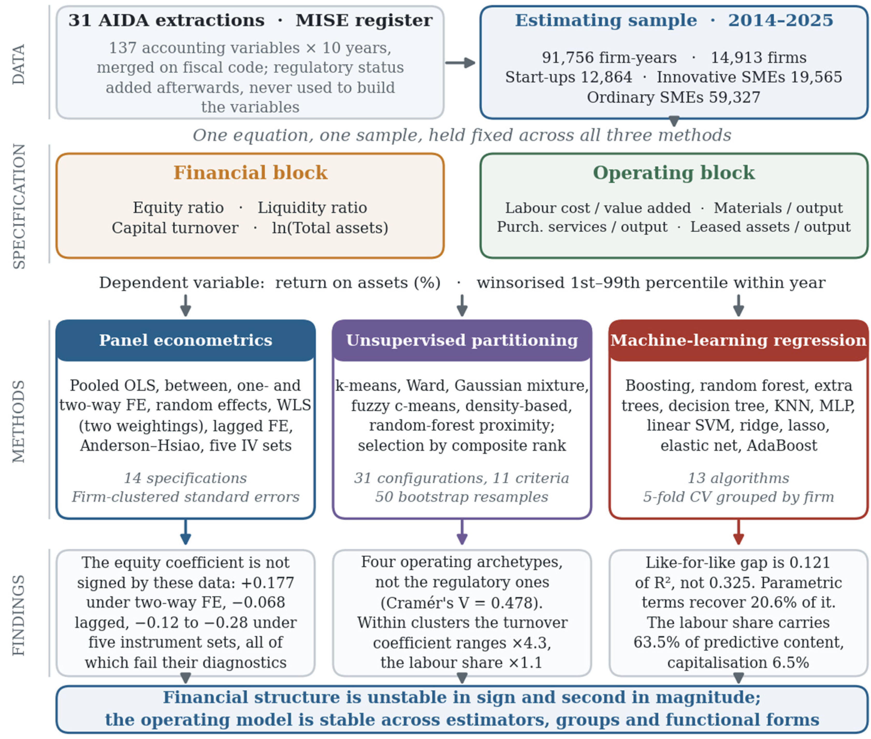
Figure 2.
Effect of a one-standard-deviation increase, four estimators.
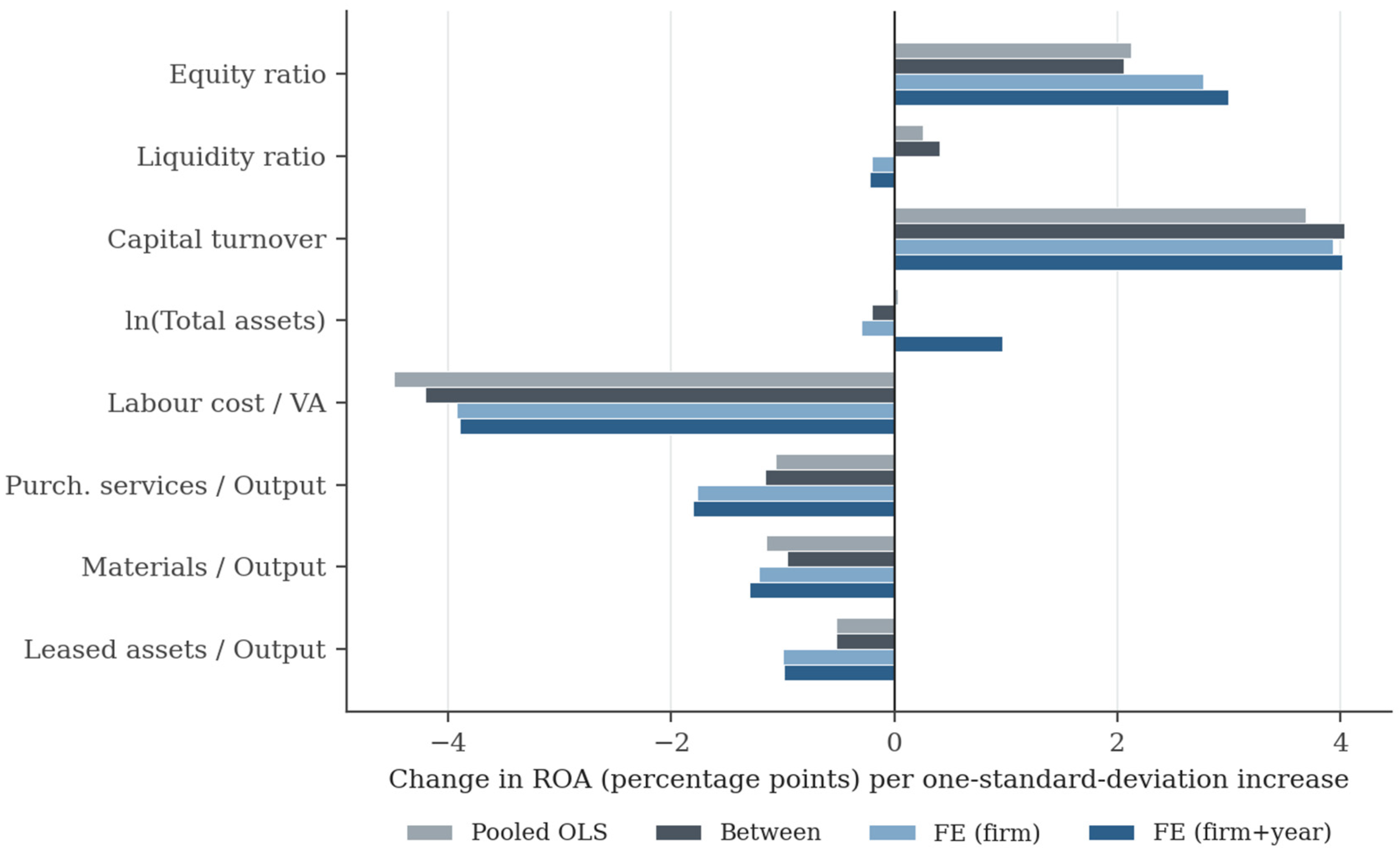
Figure 3.
Between and within estimates compared.
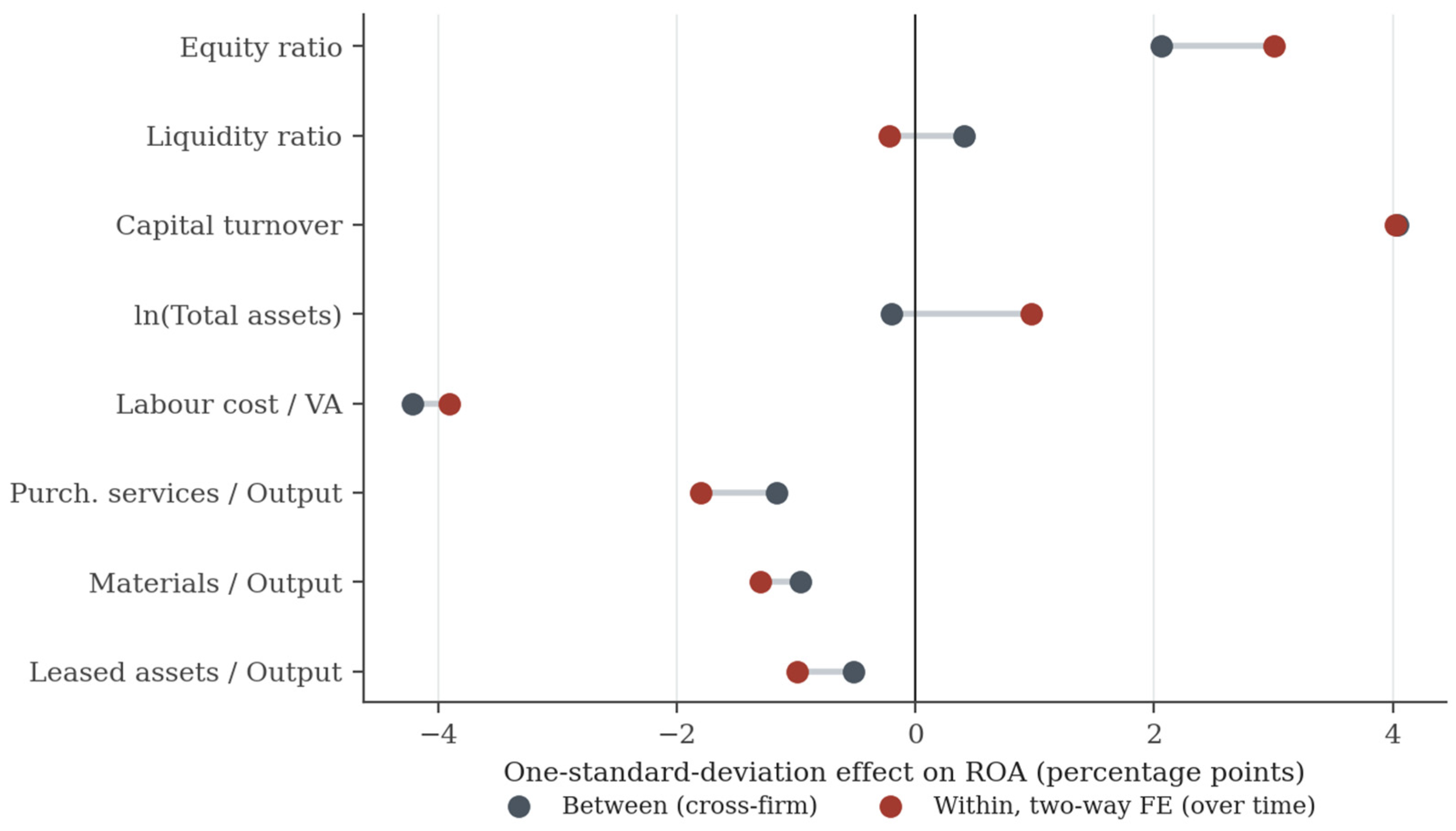
Figure 4.
The equity coefficient across every specification estimated.
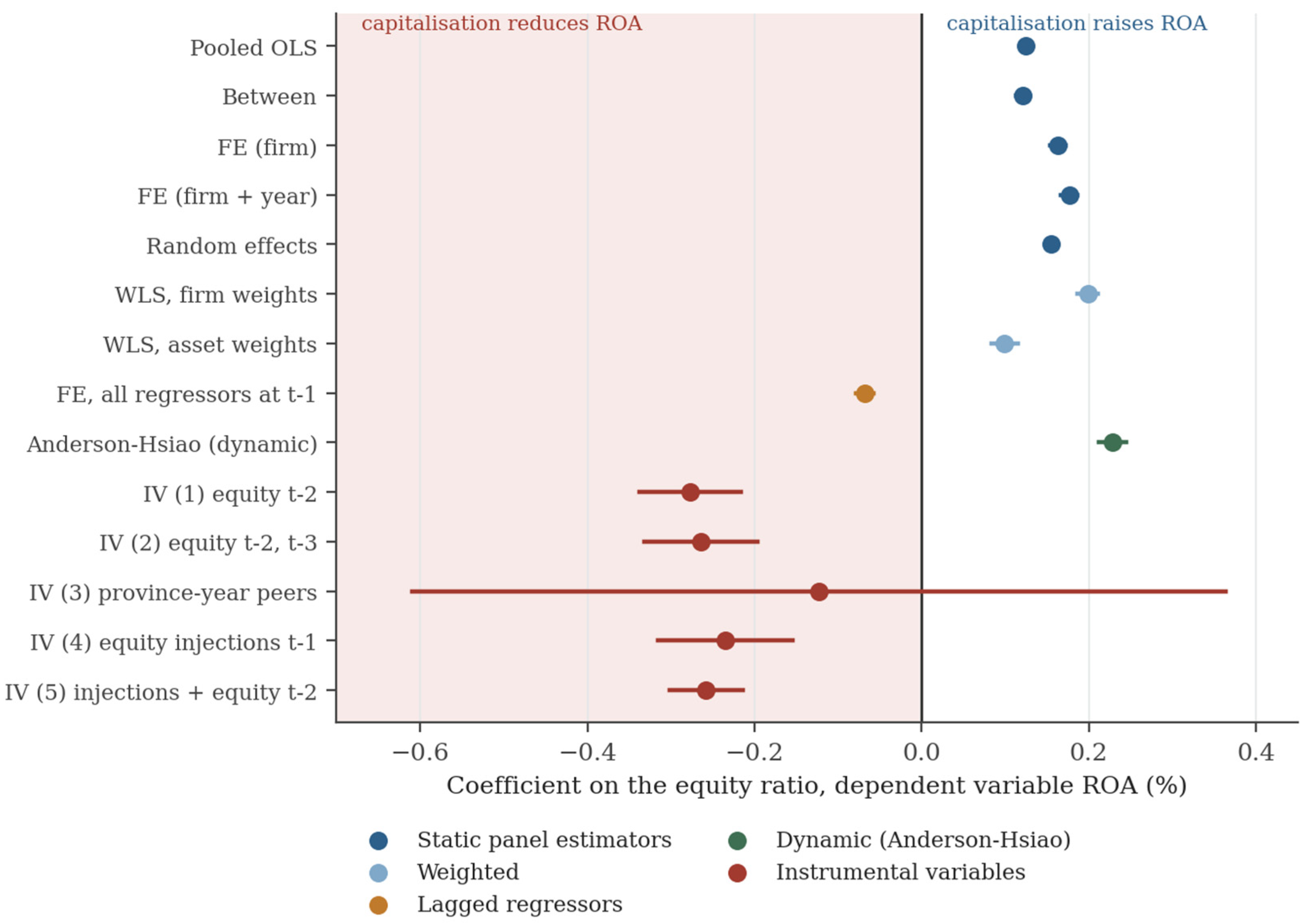
Figure 5.
Coefficients estimated separately by regulatory regime.
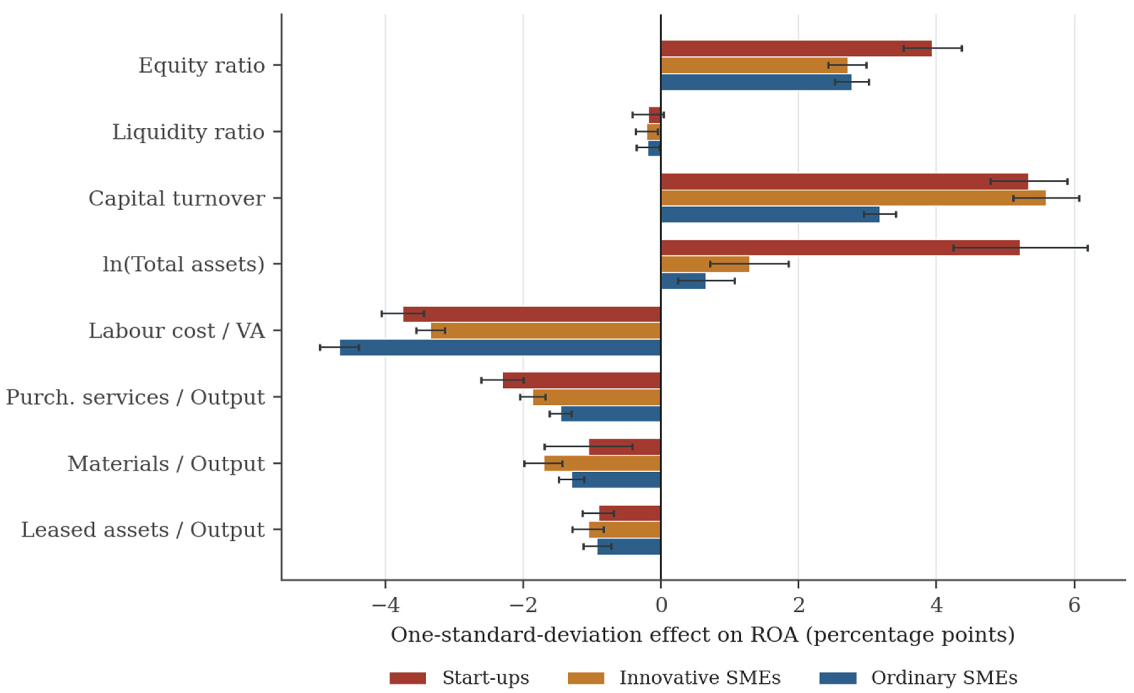
Figure 8.
Within-cluster coefficients relative to the pooled estimate.
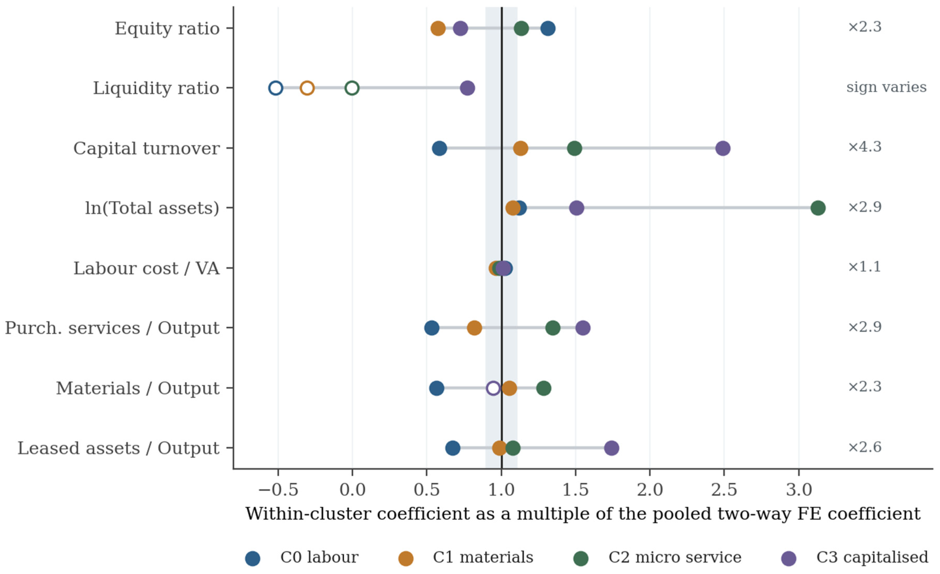
Table 1.
Synthesis of the literature.
| Research theme | Representative studies | Main gap identified | Contribution of this study |
| Capital structure and profitability in small firms (n = 28) | Benkraiem (2016); Bhawna & Sahay (2025); Ceylan (2021); Das et al. (2022); Demiraj et al. (2025); Garcia-Martinez et al. (2023); Ghasemi & Ab Razak (2017); Gonçalves et al. (2024); Govindan et al. (2023); Gutiérrez-Ponce (2024); Hussain et al. (2024); Kalash (2023); Karim et al. (2021); Khan et al. (2025); Kumar & Rao (2016); Kumar & Verma (2025); Matias & Serrasqueiro (2017); Nkosi et al. (2026); Quoc Trung (2021); Rodríguez Valencia (2025); Rokhayati et al. (2019); Shchyrba et al. (2026); Soni et al. (2023); Tran Minh Hung et al. (2026); Vu Thi & Phung (2021); Yousaf (2025); Youssef et al. (2022); Youssef et al. (2023) | Designs are national panels of a few hundred to a few thousand listed or bank-financed firms, with the equity or debt ratio as focal regressor and cost variables entering, when at all, as unexamined controls. The negative leverage coefficient is reported as settled without asking whether it survives the estimator. | Estimates the same coefficient under fourteen specifications on 91,756 firm-year observations covering 14,913 unlisted Italian firms. Reports the full range rather than a preferred column: +0.177 under two-way fixed effects, −0.068 with lagged regressors, +0.228 under Anderson–Hsiao, and between −0.12 and −0.28 across five instrument sets. |
| Endogeneity, simultaneity and identification (n = 46) | Abdalla et al. (2025); Al-Khazaleh et al. (2025); Aliakbari et al. (2025); Amarhyouz & Azegagh (2025); Artica et al. (2019); Bolarinwa et al. (2026); Boshnak (2024); Canarella & Miller (2018); Dalci (2018); Damira et al. (2022); Dsouza et al. (2025); Ernesto Martínez Avella & Andrés Hernández Salazar (2026); Goh et al. (2018); Habib (2026); Hin et al. (2026); Jolly Cyril & Singla (2020); Le et al. (2025); Li et al. (2025); Lou et al. (2025); Mansour et al. (2023); Mantzari et al. (2024); Morais Francisco (2026); Neves et al. (2026); Nguyen & Huynh (2023); Nguyen & Nguyen (2026); Novaković et al. (2025); Nyeadi et al. (2018); Pham & Ngo (2025); Pham & Nguyen (2020); Rahman & Harun (2025); Rastogi & Kumar (2024); Saiz-Sepulveda et al. (2026); Samal & Yadav (2025); Sari et al. (2026); Shakri et al. (2025); Sigalas & Gerakoudi (2025); Singh et al. (2025); Sultana & Zeya (2026); Surjanto & Ariefianto (2025); Talamas Marcos (2025); Tran & Nguyen (2025); Vengesai & Kwenda (2018); Vieira (2017); Vijayakumaran & Vijayakumaran (2019); Waheed & Bagh (2025); Xie & Yuan (2025) | Endogeneity is treated as a nuisance corrected by lagged or internal instruments and reported in a robustness column. Instrument validity is rarely tested and failures are not reported. The accounting identity linking net worth to current profit is almost never acknowledged, and the stronger identity linking the cost shares to that same profit is acknowledged nowhere. | Reports all five instrument sets with first-stage F and Hansen J, including the two that reject (J = 77.18, p < 0.001). Identifies the mechanism of failure: with ROA persistent at 0.271, the equity ratio at t−2 embeds profit at t−2. Concludes that no valid instrument for financial structure exists in these data, and applies the same scrutiny to its own leading coefficient. |
| Profit persistence and dynamic adjustment (n = 16) | Abdeljawad & Farhood (2025); Al Barakat & Ali (2026); Al-Homaidi et al. (2020); Choi et al. (2024); Doyran & Santamaria (2019); Hirsch & Hartmann (2014); Hirsch et al. (2021); Hoang et al. (2026); Jaisinghani (2016); Jouida (2018); Killins (2020); Opstad et al. (2022); Rios-Vazquez & Portela-Maseda (2026); Sinha & Vodwal (2022); Yadav et al. (2022); Yang et al. (2015) | Persistence and speed-of-adjustment are established as stylised facts but are not connected to the identification literature, where internal instruments are used as though the error were serially uncorrelated. The two bodies of work develop in parallel and cite each other rarely. | Estimates persistence at 0.271 per year and uses it to explain, rather than merely to control for, the failure of the internal instruments. Persistence is presented as the feature that makes the dynamic specification necessary and simultaneously destroys the lagged instruments. |
| Cost structure, efficiency and the operating model (n = 17) | Albaity et al. (2019); Alhassan & Ohene-Asare (2016); Bhattu-Babajee & Seetanah (2022); Campisi et al. (2019); Chadha et al. (2023); Chino (2016); Grau & Reig (2021); Lan et al. (2026); Li & Tong (2023); Maside-Sanfiz et al. (2024); Pant et al. (2026); Prakash & Nauriyal (2020); Prasad & Mondal (2025); Shyu (2013); Somya & Saripalle (2023); Spicka et al. (2017); Tripathi et al. (2024) | Operating variables are studied through efficiency scores or working-capital ratios rather than as the composition of the cost base, and are seldom placed in the same equation as financial structure. Only 27 of 2,827 retrieved records relate labour cost, value added or outsourcing to profitability, and none asks whether the resulting coefficient is behavioural or arithmetic. | Places four cost shares alongside four financial variables in one equation and rescales all eight to one-standard-deviation effects. It then shows that ROA = (VA/A)(1 − s) − D/A, so the labour-share coefficient is mechanical by construction, and measures what survives when the identity is broken by lagging: a quarter of it, at −0.0346 and significant at one per cent. The result is a measurement of how much of profitability is fixed once the cost base is known, not a behavioural claim. |
| Unsupervised classification and firm taxonomies (n = 23) | Bai & Harith (2023); Barlatier et al. (2023); Bayaraa et al. (2019); Camuffo & Poletto (2024); Cantabene & Grassi (2024); Costa et al. (2017); Davcik & Grigoriou (2020); Godley et al. (2021); Juntunen et al. (2022); Kumar et al. (2024); Lee & Hallak (2020); Linares-Mustarós et al. (2018); Ljungkvist & Andersén (2021); Meena et al. (2023); Mladenova et al. (2025); Nazarova et al. (2021); Pagaddut (2021); Risberg et al. (2023); Salina et al. (2020); Salles-Filho et al. (2023); Thomä & Bizer (2013); Williams et al. (2025); Xiao et al. (2025) | Taxonomies are selected on a single validity index, most often silhouette, which falls monotonically in k and therefore favours two-cluster solutions by construction. Partitions are described but the estimating equation is rarely re-estimated inside them. | Scores thirty-one configurations across six algorithm families on eleven validity criteria and selects by composite rank, with stability verified over fifty bootstrap resamples (mean ARI 0.9375). Re-estimates the equation within each cluster: capital turnover, which enters no identity, ranges by a factor of 4.3, while the near-invariance of the labour share (×1.1) is read as the signature of that identity rather than as structural stability. |
| Machine learning for distress, default and fraud prediction (n = 18) | Antar & Tayachi (2025); Ariza-Garzón et al. (2024); Balzano & Magrini (2026); Bijoy et al. (2026); Cheraghali & Molnár (2026); Coronell et al. (2026); Gavurova et al. (2022); Martínez et al. (2021); Mousa et al. (2025); Papíková & Papík (2024); Phothong et al. (2026); Sehgal et al. (2021); Sehgal et al. (2023); Shetty et al. (2022); Sodnomdavaa & Lkhagvadorj (2026); Wei et al. (2024); Zhang et al. (2025); Zhu et al. (2022) | Learners are evaluated on classification accuracy against a binary outcome, and the comparison with a parametric benchmark is made on raw levels, so that the gap conflates functional form with unmodelled firm heterogeneity. | Applies the learners to a continuous outcome on the same firm-demeaned data as the fixed-effects estimator. The honest gap is 0.121 rather than 0.325 of R², and the ratio falls from 1.69 to 1.29 once the between-firm variation both estimators cannot use is removed. |
| Machine learning applied to firm performance (n = 32) | Abbate et al. (2023); Ali (2026); Anton et al. (2021); Banna & Alam (2025); Bednarek et al. (2025); Deepak Kumar et al. (2024); Feng et al. (2025); Forradellas et al. (2026); Gao (2022); Garg et al. (2025); Giudici et al. (2023); Gotti et al. (2025); Gupta et al. (2025); Houssaini & Miloud (2025); Kahlen et al. (2024); Kanyepe et al. (2025); Khayer et al. (2020); Kohtamäki et al. (2024); Kristóf & Virág (2022); Mahmood et al. (2025); Mikram et al. (2025); Neha et al. (2025); Pap et al. (2022); Phuensane et al. (2026); Sengar et al. (2026); Sultana et al. (2026); Sura & Ventura (2026); Vajjhala & Strang (2024); Vašaničová et al. (2025); Xu & Sam (2025); Yang et al. (2023); Zhan et al. (2022) | Applications are prediction-oriented and report accuracy rankings; they do not ask what the accuracy gap implies for the econometric specification, nor decompose it into the kind of structure the linear form omits, nor separate genuine predictive content from accounting relations the learner reproduces exactly. | Uses the selected learner to validate rather than to predict. Parametric enrichment recovers at most 20.6 per cent of the gap with 44 terms and Friedman H-statistics peak at 0.042. Permutation importance assigns 63.5 per cent of predictive content to the labour share — part of it the accounting relation — against 6.5 per cent for capitalisation, which is mechanically unrelated to the outcome and therefore informative by its smallness. |
| Innovative start-ups and certified SMEs (n = 20) | Aiello et al. (2024); Al-Eitan et al. (2022); Amoa-Gyarteng & Dhliwayo (2023); Anderloni & Harasheh (2025); Angilella et al. (2023); Antenozio et al. (2026); Charity et al. (2019); Di Berardino & Antenozio (2026); Domma & Errico (2023); Kayani et al. (2025); Manaresi et al. (2021); Migliaccio & Pavone (2021); Minola et al. (2026); Scandurra et al. (2025); Schifilliti & La Rocca (2024); Tong & Serrasqueiro (2020); Tons & Serrasqueiro (2020); Tran & Santarelli (2014); Vannoni (2019); Zheng et al. (2016) | Evaluations of certification regimes measure average effects on growth, employment or survival while treating the financing constraint as given, and compare certified firms with matched peers rather than asking whether the structure of profit determination differs across regimes. | Estimates the equation separately for innovative start-ups, innovative SMEs and ordinary SMEs on the same sample. Wald tests reject equality of the coefficient vectors in all three pairs (87.18, 181.94, 138.08 on eight degrees of freedom), and the partition the data choose does not coincide with the register. |
Note. Two hundred studies retrieved from Scopus across eighteen queries and assigned to a single theme each, so the counts sum to the corpus. The contribution column reports the study's position after the accounting identity ofSection 7 has been taken into account. Full details are in the reference list. Note. Two hundred studies retrieved from Scopus across eighteen queries and assigned to a single theme each, so the counts sum to the corpus. Full details are in the reference list.
Table 3.
Two-way fixed effects. Dependent variable: ROA (%).
| Regressor | Coefficient | s.e. | Between | FE (firm only) |
| Equity ratio (%) | 0.1766*** | (0.0049) | 0.1210*** | 0.1629*** |
| Liquidity ratio | -0.2474*** | (0.0597) | 0.4492*** | -0.2263*** |
| Capital turnover | 5.2871*** | (0.1347) | 5.3101*** | 5.1750*** |
| ln(Total assets) | 0.6463*** | (0.1005) | -0.1359*** | -0.1997** |
| Labour cost / Value added (%) | -0.1365*** | (0.0026) | -0.1473*** | -0.1373*** |
| Purchased services / Output (%) | -0.1840*** | (0.0069) | -0.1184*** | -0.1806*** |
| Materials / Output (%) | -0.1143*** | (0.0130) | -0.0845*** | -0.1066*** |
| Leased assets / Output (%) | -0.2833*** | (0.0182) | -0.1481*** | -0.2869*** |
| Observations | 91,756 | 14,913 | 91,756 | |
| Within R² | 0.4232 | 0.4911 | 0.4161 |
Note. Firm-clustered standard errors. *** p<0.01, ** p<0.05, * p<0.10. The two-way specification includes year dummies; between is estimated on firm means, and its R² refers to cross-firm variance and is not comparable with the within figures. The full comparison across five estimators isTable A1.
Table 5.
Cluster profiles, medians of the original variables.
| Variable | C0 labour | C1 materials | C2 micro service | C3 capitalised |
| ROA (%) | 3.03 | 4.72 | 7.36 | 10.23 |
| Equity ratio (%) | 17.29 | 33.22 | 34.71 | 70.10 |
| Liquidity ratio | 1.22 | 1.08 | 1.31 | 3.70 |
| Capital turnover | 1.23 | 1.03 | 0.69 | 0.59 |
| ln(Total assets) | 7.58 | 9.75 | 4.79 | 5.60 |
| Labour cost / Value added (%) | 89.63 | 67.55 | 0.63 | 35.23 |
| Purchased services / Output (%) | 29.94 | 18.88 | 57.35 | 34.94 |
| Materials / Output (%) | 3.04 | 47.43 | 0.81 | 0.82 |
| Leased assets / Output (%) | 3.69 | 1.95 | 0.68 | 1.15 |
| Firms | 5,067 | 4,023 | 3,615 | 2,224 |
| Share of firms (%) | 33.9 | 26.9 | 24.2 | 14.9 |
Note. Medians of firm-level decade medians. k-means, k = 4, on the nine standardised variables. Cluster labels are ours and describe the dominant feature of each profile; they play no part in the procedure.
Table 12.
Value added over total assets and the labour-share coefficient, by archetype.
| Cluster | Firms | VA / A p25 | VA / A median | Implied slope | Estimated coefficient | Ratio |
| C0 labour | 5,056 | 0.297 | 0.602 | −0.602 | −0.1403*** | 0.23 |
| C1 materials | 4,109 | 0.203 | 0.292 | −0.292 | −0.1317*** | 0.45 |
| C2 micro service | 3,649 | 0.093 | 0.217 | −0.217 | −0.1347*** | 0.62 |
| C3 capitalised | 2,406 | 0.176 | 0.417 | −0.417 | −0.1383*** | 0.33 |
| Range, largest / smallest | — | — | 2.8× | 2.8× | 1.07× | — |
Note. Median value added over total assets computed on firm-year observations within each cluster; quartiles on firm-level medians. The implied slope is the negative of the cluster median, which is what the identity predicts exactly. Estimated coefficients are the two-way fixed-effects estimates of Table A5. *** p<0.01. Cluster membership is reconstructed by reapplying the procedure of Section 5 — decade medians of the nine standardised variables, k-means at k = 4 — to the 94,258 firm-year observations on 15,220 firms for which all nine variables are present, a sample 2.7 per cent larger than that of Table 2. The reconstruction reproduces the published partition closely: cluster shares are 33.2, 27.0, 24.0 and 15.8 per cent against 33.9, 26.9, 24.2 and 14.9 in Table 5, and the profile medians agree to within a few tenths on every variable. The comparison in the last two columns is therefore between a value added ratio computed on the reconstructed partition and coefficients estimated on the original one; the conclusion turns on a ratio of 2.8 against 1.07 and is not sensitive to a discrepancy of this size.
Table 9.
Results by method and their relation to the existing literature.
| Method | Result obtained | Relation to the literature | Reading | Studies concerned |
| Panel econometrics | Capitalisation is positively and significantly associated with ROA under all five static estimators (+0.121 to +0.177) | In line | Confirms the sign that is the settled result of the small-firm literature, on a population of unlisted firms it has rarely covered | Matias & Serrasqueiro (2017); Dalci (2018); Quoc Trung (2021); Kalash (2023); Youssef et al. (2023); Gonçalves et al. (2024); Bhawna & Sahay (2025) |
| The same coefficient turns to −0.068 when regressors are lagged and to between −0.12 and −0.28 under five instrument sets; the sign is not identified | In opposition | Contradicts the practice of reporting one instrumented column as confirmation; the disagreement between treatments is the result, not a footnote | Canarella & Miller (2018); Vijayakumaran & Vijayakumaran (2019); Samal & Yadav (2025); Dsouza et al. (2025); Saiz-Sepulveda et al. (2026) | |
| Profitability persists at 0.271 per year, which is why lagged capitalisation cannot instrument current capitalisation (Hansen J = 77.18) | Contrasting | Accepts the persistence finding and turns it against the identification strategy the same literatures use, a connection neither strand draws | Hirsch & Hartmann (2014); Yang et al. (2015); Hirsch et al. (2021); Sinha & Vodwal (2022); Choi et al. (2024) | |
| Coefficient vectors differ across regulatory regimes (Wald 87.18, 181.94, 138.08 on 8 d.f.) | Contrasting | Certification tracks a difference in the structure of profit determination, not only in its average level, which treatment-effect designs cannot detect | Vannoni (2019); Manaresi et al. (2021); Migliaccio & Pavone (2021); Angilella et al. (2023); Aiello et al. (2024); Anderloni & Harasheh (2025) | |
| Accounting identity | ROA = (VA/A)(1 − s) − D/A, so ∂ROA/∂s = −VA/A exactly; four of the eight regressors are subtracted items divided by the aggregates they are subtracted from | In opposition | Cost shares cannot be read as behavioural coefficients in an equation whose dependent variable is built from the same statement, which the operating-side literature does without comment | Campisi et al. (2019); Grau & Reig (2021); Bhattu-Babajee & Seetanah (2022); Chadha et al. (2023); Tripathi et al. (2024) |
| Median VA/A is 0.353, so the identity implies −0.355 against an estimate of −0.1365; the lagged coefficient of −0.0346*** would require 0.035 | Contrasting | The identity over-predicts the estimate by a factor of two to three, so the coefficient is the identity attenuated rather than the identity, and a quarter of it survives the identity being broken | Grau & Reig (2021); Prakash & Nauriyal (2020); Yousaf (2025) | |
| Across the four archetypes VA/A ranges by a factor of 2.8 while the coefficient ranges by 1.07, from −0.132 to −0.140 | In opposition | Neither the convention that coefficient stability evidences structure nor the objection that it is arithmetic can be settled by assertion; here the identity fixes a magnitude, the magnitude is tested, and the stability is not mechanical | Canarella & Miller (2018); Das et al. (2022); Kalash (2023); Sultana et al. (2026) | |
| Unsupervised clustering | Four operating archetypes emerge from accounting data alone; k-means at k = 4 selected on eleven criteria, ARI 0.9375 over 50 resamples | In line | Reproduces the finding that firms fall into stable financial-operational types, with a selection protocol stricter than the single-index norm | Linares-Mustarós et al. (2018); Bayaraa et al. (2019); Anton et al. (2021); Ljungkvist & Andersén (2021); Juntunen et al. (2022); Kristóf & Virág (2022) |
| Silhouette falls monotonically in k for every partitional method, so silhouette-based selection returns two clusters by construction | In opposition | Challenges the dominant selection practice: the number of groups reported in much of this literature is an artefact of the index chosen | Bayaraa et al. (2019); Salina et al. (2020); Bai & Harith (2023); Williams et al. (2025); Vašaničová et al. (2025) | |
| The turnover coefficient ranges ×4.3 across clusters and the labour share ×1.1; the partition does not coincide with the register (Cramér's V = 0.478) | Contrasting | The turnover dispersion is a genuine failure of the pooled vector; the labour-share invariance survives the cross-cluster test and is a property of the relationship, so the partition serves as a diagnostic and not only as a description | Davcik & Grigoriou (2020); Godley et al. (2021); Salles-Filho et al. (2023); Mladenova et al. (2025) | |
| Machine-learning regression | Tree ensembles beat the linear family on the same data (R² 0.798 against 0.473 on levels); histogram gradient boosting selected on a five-indicator battery | In line | Confirms the accuracy ordering repeatedly reported for accounting data, including the weakness of linear SVM and the instability of AdaBoost | Shetty et al. (2022); Pap et al. (2022); Gavurova et al. (2022); Giudici et al. (2023); Papíková & Papík (2024); Cheraghali & Molnár (2026) |
| On firm-demeaned data the gap is 0.121, not 0.325; the ratio falls from 1.69 to 1.29 | In opposition | The headline advantage reported in levels comparisons is mostly firm heterogeneity that fixed effects already absorb, not functional form | Vajjhala & Strang (2024); Mahmood et al. (2025); Sultana et al. (2026); Sengar et al. (2026) | |
| Permutation importance assigns 63.5% of predictive content to the labour share and 6.5% to capitalisation; H² peaks at 0.042 | Contrasting | Part of the 63.5% is the accounting relation a learner reproduces almost exactly; the 6.5% is not, since capitalisation is mechanically unrelated to the outcome and is therefore informative by its smallness | Antar & Tayachi (2025); Ariza-Garzón et al. (2024); Balzano & Magrini (2026) |
Note. “In line” denotes a result that reproduces the established finding; “contrasting” a result that qualifies or reframes it; “in opposition” a result that contradicts the established finding or the practice that produces it. The second block reports the tests ofSection 7, one of which reverses a reading advanced earlier in this paper. Studies listed are those from the reviewed corpus most directly concerned.
Disclaimer/Publisher’s Note: The statements, opinions and data contained in all publications are solely those of the individual author(s) and contributor(s) and not of MDPI and/or the editor(s). MDPI and/or the editor(s) disclaim responsibility for any injury to people or property resulting from any ideas, methods, instructions or products referred to in the content. |
© 2026 by the authors. Licensee MDPI, Basel, Switzerland. This article is an open access article distributed under the terms and conditions of the Creative Commons Attribution (CC BY) license.
Copyright: This open access article is published under a Creative Commons CC BY 4.0 license, which permit the free download, distribution, and reuse, provided that the author and preprint are cited in any reuse.