

Submitted:
08 September 2026
Posted:
08 September 2026
You are already at the latest version
Abstract
Fashion enterprises face demand uncertainty from seasonality, short product life cycles, and dense color-size variation: excessive ordering enlarges aged-inventory risk, whereas insufficient ordering causes stockouts. This study develops and validates a manager-assisted hybrid decision support system (DSS) integrating demand forecasting, reorder-candidate identification, aged-inventory risk detection, and ranking-based prioritization. Operational data from a Korean fashion enterprise (4,130,603 sales and 5,065,027 order records) were reconstructed into a style-level monthly panel of 263,260 observations and split chronologically into training (2012–2014), validation (2015), and test (2016) periods to prevent leakage. Three baselines and nine data-driven models, Random Forest, Histogram Gradient Boosting, LightGBM, a two-stage Hurdle LightGBM, LSTM, Transformer, TimeMixer, TimeXer, and CrossLinear, were benchmarked, their outputs then combined with current-month sales signals and an inventory-comparison rule inside the DSS. On the 2016 test data, the DSS attained a Weighted Absolute Percentage Error of 0.6477, reorder F1-score of 0.7983, Hit@50 of 47.04%, and NDCG@50 of 75.12%, a balance no single model achieved. A policy simulation indicated that DSS-guided ordering could cut inbound order quantity by 25.9% and long-term inventory risk by 23.0%, at the cost of a 39.5% rise in shortage quantity. Forecasting accuracy alone is therefore insufficient for deploying artificial intelligence in inventory decisions.
Keywords:
demand forecasting
; decision support system
; aged inventory
; reorder decision
; fashion retail
; machine learning
; LightGBM
; ranking recommendation
; supply chain management
; time-series forecasting
1. Introduction
1.1. Background and Motivation
Manufacturing and distribution enterprises make continuous, interdependent decisions across the entire product life cycle, spanning product planning, production, ordering, inbound logistics, storage, sales, returns, and carry-over inventory management [1,2,3,4,5,6,7]. Fashion manufacturing and distribution firms face this challenge in an especially acute form, because short product life cycles, strong seasonality and trend sensitivity, and highly diversified color-size combinations jointly generate substantial demand uncertainty [3,4,5,6,7]. Even items that belong to the same style may exhibit markedly different sales trajectories depending on color, size, price, discount status, sales channel, and inventory availability. Under these conditions, replenishment practices based solely on historical sales aggregation or managerial experience are increasingly insufficient for responding to fast-moving market demand.
Enterprise information systems, including Point-of-Sale (POS), Order Management, and Logistics Management Systems, have accumulated large volumes of transactional data [1,2]. However, these systems are designed primarily for operational processing rather than managerial decision-making, so that sales, order, product-master, and store-master records must be integrated through an explicit analytical framework before they can support demand forecasting, reorder-candidate identification, aged-inventory risk detection, merchandise planning, and logistics decisions [1,2,8,9,10,11]. Because fashion products lose marketability rapidly once a selling season ends, excessive ordering tends to produce long-term inventory accumulation and aged-inventory risk, whereas insufficient ordering increases stockouts and lost sales opportunities [8,9,10,11]. Consequently, the central problem in integrated manufacturing and distribution decision-making is not simply to identify which products will sell well, but to convert forecasts into actionable managerial information by jointly accounting for current inventory, procurement lead time, expected replenishment, service-level requirements, and long-term inventory risk [8,9,10,11,12,13,14].
1.2. Problem Statement and Research Gap
Prior demand-forecasting research has concentrated primarily on minimizing the discrepancy between predicted and realized sales [12,13,14]. Predictive accuracy is undeniably important, yet a single forecast value is insufficient to determine replenishment quantities in practice, because actual reorder decisions must simultaneously reflect minimum order quantities, production feasibility, distribution-center and store inventory status, season-end schedules, pricing and discount policy, new-product launch plans, and return or consignment structures. Fashion products are further managed at the individual color-size level, so sparse-demand conditions with frequent zero-sales months are common [3,4,5,6,7,15,16], a pattern that limits the practical value of any single point-forecast model and makes it unwise to convert model outputs directly into automatic replenishment orders.
Artificial intelligence should therefore be treated not as a mechanism for fully automating replenishment, but as a decision-support technology that helps managers and inventory planners make better-informed decisions [17,18,19,20,21,22]. An AI-based decision support system (DSS) should identify priority product groups, recommend reorder candidates, flag potential long-term inventory risk, and expose the analytical evidence behind each recommendation, rather than silently determine order quantities [17,18,19,20,21,22,23,24,25]. This orientation is consistent with the classical view of decision support systems as tools that augment, rather than replace, managerial judgment [19,20,21,22], and it is reinforced by the broader human-centered artificial intelligence and explainable-AI literature, which emphasizes that automated recommendations gain practical value only when they remain interpretable and reviewable by the people who act on them [17,18,23].
Building on an earlier case study that examined, from an implementation perspective, how an AI-based decision support system could strengthen the competitiveness of a footwear and fashion enterprise through ABC analysis, demand forecasting, and distribution-center visualization [26], the present study extends that line of work into a fully empirical, multi-model, multi-year analysis. Specifically, it addresses a gap that spans three strands of prior literature that have largely developed in isolation: (i) fashion demand-forecasting studies that benchmark predictive accuracy without connecting forecasts to reorder or inventory-risk decisions [3,4,5,6,7,27,28,29,30]; (ii) inventory-theoretic studies of obsolescence and intermittent demand that seldom incorporate modern machine-learning forecasts [8,9,10,11,15,16]; and (iii) recent deep-learning and exogenous-variable time-series architectures that are typically evaluated on forecasting-error benchmarks rather than on decision-support tasks such as reorder-candidate ranking [31,32,33,34,35,36,37,38,39,40].
1.3. Research Objectives and Contributions
The purpose of this study is to design and empirically validate a manager-assisted hybrid DSS that integrates demand forecasting, reorder-candidate identification, aged-inventory risk detection, and ranking-based prioritization of review candidates, using multi-year operational data from a fashion manufacturing and distribution enterprise. Five research questions guide the study:
RQ1. Can product-master, sales-detail, order-detail, and store-master data from a fashion manufacturing and distribution enterprise be integrated to construct a style-level monthly panel suitable for an AI-based DSS?
RQ2. How do Random Forest, Histogram Gradient Boosting, LightGBM, Hurdle LightGBM, LSTM, Transformer, TimeMixer, TimeXer, and CrossLinear differ in demand-forecasting accuracy and reorder-decision performance under sparse-demand, strongly seasonal fashion data?
RQ3. Can a hybrid DSS that combines a forecasting module with current-month sales signals and an inventory-comparison rule achieve a better balance between reorder-candidate identification and demand-forecasting performance than a single model or a conventional baseline?
RQ4. Can operational aged-inventory risk candidates be identified effectively by combining elapsed time since product launch, current inventory, and forecasted future demand?
RQ5. Can a Top-50 ranking-recommendation mechanism serve as an effective DSS function for prioritizing reorder and aged-inventory risk candidates that require managerial review?
The contributions of this study are fourfold. First, it extends demand-forecasting research from a prediction-centered perspective toward a decision-support perspective by jointly evaluating forecasting-error metrics together with reorder precision, recall, F1-score, ranking quality, and quantity-recall metrics. Second, it proposes a dual-level analytical structure, style-level for predictive stability and detailed color-size level for operational executability, that directly addresses the sparsity and hierarchical structure of fashion-product data. Third, it benchmarks three operational baselines and nine data-driven models, including three recently proposed exogenous-variable-aware architectures (TimeMixer, TimeXer, and CrossLinear), under an identical evaluation protocol and interprets their comparative roles according to specific decision-support tasks rather than a single aggregate ranking. Fourth, it defines aged-inventory risk as an operational, ex-ante candidate for managerial review rather than an accounting-confirmed loss, and demonstrates through offline policy simulation that a hybrid DSS can reduce ordering volume and long-term inventory risk while revealing an explicit trade-off with shortage risk.
1.4. Paper Organization
The remainder of this paper is organized as follows. Section 2 reviews related work on fashion demand forecasting, inventory management, machine-learning and deep-learning forecasting models, and decision support systems. Section 3 describes the research data and preprocessing pipeline. Section 4 presents the proposed manager-assisted hybrid DSS. Section 5 defines the evaluation metrics. Section 6 reports the experimental results. Section 7 discusses the practical implications and limitations of the study, and Section 8 concludes the paper.
2. Related Work
Fashion demand forecasting has long been recognized as unusually difficult because of short selling seasons, trend sensitivity, and a combinatorial explosion of color-size variants [3,4,5,6,7]. Survey evidence indicates that classical statistical methods, which assume stable and continuous demand, tend to underperform on fashion assortments precisely because a large share of color-size items experience intermittent or zero demand in any given month [3,15,16]. Supply-chain-oriented studies of fast-fashion retailing show that shortening the forecast-to-replenishment cycle and improving responsiveness can materially reduce both markdowns and stockouts [5,6,7], which motivates treating forecasting as one input to a broader inventory-decision problem rather than as a self-contained objective. Several Korean studies have examined apparel sales patterns in relation to product attributes, weather, discount rate, and weekend effects [27,28,29,30], confirming that observable product and contextual attributes carry meaningful explanatory power beyond historical sales alone; the present study incorporates this insight by using product category, season, color, price level, and elapsed time since launch as explicit model inputs and interpretive context for managerial review, rather than as a separate weather-driven forecasting task.
Classical inventory theory frames replenishment as a trade-off between holding costs, shortage costs, and order costs, most explicitly in the single-period newsvendor model and its extensions [8,9]. This literature also provides the conceptual foundation for treating slow-moving and obsolete inventory as a distinct risk category rather than as an undifferentiated component of on-hand stock [10,11]. Obsolescence-oriented studies typically link forecasting error directly to the probability that inventory will not be sold before it loses value [10,11], which parallels the aged-inventory risk construct used in this study; however, this line of work rarely operationalizes obsolescence risk using enterprise-scale, item-level transactional data of the kind analyzed here. The present study builds on this theoretical foundation but departs from it in one important respect: rather than assuming that individual inventory units can be traced from receipt to disposition, it defines aged-inventory risk at the operational style level, based on elapsed time since launch and the gap between current inventory and forecasted future demand, because real operational databases identify color-size-option combinations rather than serialized inventory units.
Tree-based ensemble methods, including Random Forest [41], gradient boosting machines [42], and their efficient modern implementations such as XGBoost [43], CatBoost [44], and LightGBM [45], are widely used for tabular demand-forecasting problems because they handle heterogeneous, non-linear feature interactions without extensive manual feature transformation [46]. Machine-learning approaches of this kind have repeatedly shown measurable accuracy gains over classical statistical methods in supply-chain demand-forecasting benchmarks [47]. Because fashion-product panels contain a high proportion of zero-sales observations, hurdle and two-part count-data models that separate the occurrence of positive demand from its conditional magnitude [48] are particularly relevant; this study adapts that idea into a two-stage Hurdle LightGBM that first classifies sales occurrence and then regresses conditional demand quantity.
Sequential deep-learning architectures, beginning with Long Short-Term Memory (LSTM) networks [31] and the Transformer and its self-attention mechanism [32], provide an alternative approach that can learn temporal dependencies directly from raw sequences. Building on this foundation, a growing body of recent work has proposed specialized time-series architectures, including Temporal Fusion Transformers for interpretable multi-horizon forecasting [36], Informer [38], Autoformer [39], and FEDformer [40] for long-sequence forecasting, and, most directly relevant to this study, TimeMixer, which mixes temporal representations across multiple scales [33]; TimeXer, which augments Transformer-style forecasting with exogenous variables [34]; and CrossLinear, which uses a lightweight cross-correlation embedding to fuse endogenous and exogenous series within a predominantly linear architecture [35]. General surveys of deep learning for time-series forecasting [37] and of forecasting theory and practice more broadly [14] confirm that no single family of models dominates across tasks, which motivates the multi-model, multi-task comparison adopted in this study. Because the training, validation, and test partitions in this study are separated chronologically, the methodological literature on out-of-sample evaluation and cross-validation for time-series predictors [49,50,51] directly informs the evaluation protocol described in Section 3.
The conceptual foundation for decision support systems dates to early work distinguishing structured, computable decisions from unstructured decisions that require human judgment supported by information systems [19], and to subsequent frameworks for developing DSS architectures [20] and for understanding data-driven DSS more specifically [21]. Critical reviews of the DSS literature have repeatedly emphasized that a system’s practical value depends on whether its outputs are actionable and trusted by decision-makers, not merely on its statistical accuracy [22], a concern echoed in the explainable-AI literature on transparency and responsible AI [23] and in guidelines for human-AI interaction that stress reviewability and graceful hand-off of control to the human operator [17,18]. The present study operationalizes these principles by presenting ranked candidates together with their supporting evidence rather than automated order quantities.
Because the proposed DSS ultimately produces a ranked list of review candidates, this study also draws on the information-retrieval and recommender-systems literature. Cumulative gain-based ranking evaluation [25] underlies the NDCG@50 metric used in this study, general treatments of learning to rank [52] and hybrid recommender systems [53] motivate the combination of forecasted demand, current-month sales signals, and inventory-comparison rules into a single ranking score, and established practices for evaluating collaborative-filtering and top-N recommendation quality [24,54,55] inform the use of Hit@K alongside quantity-recall metrics. Framing reorder-candidate prioritization as a top-K ranking problem, rather than as an unranked binary classification problem alone, distinguishes this study from most prior fashion-forecasting work and directly supports RQ5.
3. Data and Preprocessing
3.1. Data Sources
The empirical analysis uses anonymized, multi-year operational data from a domestic fashion manufacturing and distribution enterprise. As summarized in Table 1, the source data comprise four record types: Product Master (28,278 rows), containing product code, name, gender, season, category, and price; Sales Detail (4,130,603 rows), containing POS sale date, product code, sales quantity, and sales amount; Order Detail (5,065,027 rows), containing internal replenishment order and inbound-logistics transactions; and Store Master (1,347 rows), containing store codes and attributes used as reference data for verifying transaction consistency. Sales Detail records serve as the basis for target-variable construction, Order Detail records support reconstruction of the order and inventory flow, Product Master supplies attribute information used for interpretation, and Store Master provides consistency checks; store-level modeling itself was outside the scope of this study, which focuses on style-level forecasting and DSS design.
3.2. Unit of Analysis and Panel Construction
Detailed operational product codes (GOODS_CD), which represent individual color-size combinations, provide the practical granularity required for field-level inventory review, but they also contain frequent zero-sales months and are consequently too sparse for stable model training. To address this trade-off, the study adopts a dual-level analytical framework: the upper-level style code (STYLE_CD) is used as the primary forecasting and modeling unit, while detailed operational product codes are retained for a secondary, detailed-level verification of practical executability (Section 6.6). Transaction-level records were aggregated into monthly panels first at the detailed-item level (1,163,307 rows) and then at the style level (263,260 rows). Reconstructing the product launch month, applying a three-month lead-time assumption, and rebuilding the inventory flow from order and sales histories yielded 187,392 supervised-learning samples, each built on a twelve-month history window.
3.3. Feature Engineering
Following standard practice for engineering lagged, moving-average, and volatility-based predictors from panel data [56], for each style-month observation the model inputs combine current-state features (current inventory, months elapsed since launch, current-month sales), historical pattern features (lagged sales and order quantities), moving-average and volatility features computed over trailing windows, and product-attribute features (category, gender, season, color, and price level).
More specifically, the input variables were organized into six feature groups, summarized in Table 2. Current-state features (current sales, stock, and order status) describe the operating status at the reference month. Historical-lag features (sales and orders at one, three, six, and twelve months prior) capture past demand and replenishment flow. Rolling-statistics features (recent sales mean, sum, and standard deviation) summarize short-term trend and volatility. Zero-demand-structure features (consecutive zero-sales months and recent sales signal) explicitly represent sparse demand and long non-sales periods, which are otherwise easily conflated with genuinely low-demand items. Product-attribute features (gender, season, category, and base price) encode fixed product characteristics, and life-cycle features (months since launch and a long-run operation flag) represent each style’s position within its selling life cycle. Missing values were handled according to the semantic meaning of each variable rather than uniform zero-filling: missing sales or order quantities were interpreted as an absence of transactions and set to zero, whereas missing product attributes were supplemented through product-code linkage where possible and otherwise retained as a distinct category, because conflating a true zero with missing information could otherwise bias the forecasting and interpretation modules alike.
Missing values arising from newly launched styles or incomplete historical windows were handled through explicit indicator variables and appropriate default-value imputation rather than naive zero-filling, so that the absence of history is not conflated with the presence of zero demand.
3.4. Data Leakage Prevention and Chronological Splitting
Because the proposed DSS is intended to support decisions made with only currently available information, any input variable that could only be observed after the forecasting reference month was excluded, and all identifier variables were omitted from model inputs to prevent the models from memorizing product-code-specific patterns rather than learning transferable demand structure. The dataset was then split strictly chronologically, as summarized in Table 3, with training data drawn from 2012–2014 (70,199 samples), validation data from 2015 (52,898 samples) used for model and policy-threshold selection, and test data from 2016 (64,295 samples) reserved exclusively for final, independent performance evaluation. Because temporal leakage is a well-documented threat to the validity of time-series evaluation [49,50,51,57], the validation and test roles were kept strictly separate throughout model development: test-period outcomes were never used to retune models or adjust DSS decision thresholds, which is essential for the test-period results reported in Section 6 to reflect genuine out-of-sample generalization rather than optimistic bias.
4. Proposed Manager-Assisted Hybrid DSS
4.1. System Overview
Figure 1 summarizes the overall research framework. Product-master, sales-detail, order-detail, and store-master records are integrated and reconstructed into the style-level monthly panel described in Section 3. A set of comparative forecasting models is then trained on this panel to produce future-demand estimates. Rather than converting these estimates directly into automatic order quantities, the proposed hybrid DSS decision layer combines the forecasting module with a current-month sales signal and an inventory-comparison rule to compute an estimated shortage quantity for every style-month, which in turn drives three managerial outputs: a ranked reorder-candidate list, a separately ranked aged-inventory risk candidate list, and a Top-K managerial review list that prioritizes the candidates most likely to require immediate attention. This architecture reflects the core design principle of the study: AI outputs are treated as decision-support information rather than as automated ordering decisions.
4.2. Comparative Forecasting Models
Three operational baselines and nine data-driven models were evaluated under an identical training, validation, and test protocol, spanning the four model families summarized in Table 4. (1) Simple baselines - an All-Zero baseline, a Current-Month Sales baseline that carries the most recent month’s sales forward, and a Three-Month Moving-Average baseline - establish lower bounds on achievable performance and represent decision rules already used informally in practice. (2) Tabular machine-learning models - Random Forest [41], Histogram Gradient Boosting [42], and LightGBM [45] - learn non-linear relationships between engineered features and future demand. (3) A two-stage Hurdle LightGBM [48] separately models the probability of positive demand, P(y > 0), and the conditional demand quantity given positive demand, E[y | y > 0], such that the final forecast is
ŷ = P(y > 0) × E[y | y > 0]
This decomposition mirrors the two-step managerial workflow of first deciding whether a style warrants review and then estimating the required quantity, and it is designed to address the frequent zero-sales months characteristic of fashion-product data. (4) Sequential deep-learning and recent time-series models - LSTM [31], Transformer [32], and three recently proposed architectures, TimeMixer [33], TimeXer [34], and CrossLinear [35] - capture temporal dependencies directly from historical sequences. TimeMixer combines representations extracted at multiple temporal scales; TimeXer augments sequence modeling with exogenous variables such as product category, season, price range, and current inventory; and CrossLinear concatenates endogenous and exogenous sequences and applies a lightweight one-dimensional cross-correlation embedding before a patch-based linear prediction head, combining the two representations as
where hendo is the endogenous temporal representation, hcross is the cross-correlation representation extracted from the concatenated endogenous-exogenous input, and α is a learnable weighting parameter that controls their relative contribution. All tabular models were implemented using standard open-source machine-learning libraries [58]. Model selection criteria combined forecasting accuracy, reorder-candidate identification performance, ranking quality, aged-inventory risk identification, and computational resource consumption (Section 6), rather than forecasting error alone.
z = α · hendo + (1 − α) · hcross
4.3. Hybrid Decision Layer
Figure 2 details the hybrid decision layer that converts forecasting-module outputs into managerial candidates. Component (B), the current-month sales signal, reflects the empirical observation that recent realized sales carry independent information about near-term reorder need beyond what a monthly-horizon forecast alone captures. Component (C), the inventory-comparison rule, subtracts current on-hand and in-transit inventory from forecasted future demand to obtain an estimated shortage quantity for each style; a positive value places the style into the candidate pool, and candidates are ranked by the magnitude of the estimated shortage. Because the reorder-decision component of the Hybrid DSS uses the current-month sales signal as its classification boundary while the forecasting module continues to calibrate the predicted demand quantity, the Hybrid DSS in Table 5 shares its reorder precision, recall, and F1-score with the Current-Month Sales baseline while achieving a distinctly lower WAPE and MAE (Section 6.1); this pattern is a designed property of the architecture rather than a coincidence, and it illustrates how the hybrid layer decouples quantity calibration from candidate identification. This separation preserves interpretability while refining quantity estimates for the candidates presented during subsequent managerial review.
4.4. Aged-Inventory Risk Identification
Because operational product codes identify color-size-option combinations rather than serialized inventory units, this study defines aged-inventory risk as an operational construct rather than an accounting-confirmed loss. A style is flagged as an aged-inventory risk candidate when (i) a predefined period has elapsed since its launch month and (ii) its current inventory exceeds forecasted future demand over the applicable horizon. Styles satisfying both conditions are presented to managers as candidates warranting discounting, inter-store transfer, discontinuation, restriction of additional ordering, or promotional review, rather than as inventory that has already been written off. This ex-ante framing extends the inventory-obsolescence literature [10,11] from an accounting and forecasting-error perspective toward an actionable, ranking-based managerial review mechanism.
4.5. Top-Ranked Candidate Recommendation and Product-Attribute Interpretation
Because inventory managers cannot review every product with equal depth, the DSS constructs a Top-K candidate list (K = 50 in the main experiments) by ranking styles according to estimated shortage quantity within evaluation groups defined by month, season, gender, and product subcategory, evaluated using Hit@K, NDCG@K, and quantity-recall metrics (Section 5). To keep these rankings interpretable, every candidate is presented together with product-attribute context, category, season, color, price level, and months elapsed since launch, so that managers can assess, for example, whether a candidate entering its peak season warrants a different response than an otherwise similar off-season candidate. This attribute-based interpretation layer is intended to bridge quantitative model output and the contextual operational knowledge that managers bring to the final decision, consistent with the human-centered and explainable-AI principles discussed in Section 2.4 [17,18,23].
5. Evaluation Metrics
Model performance is evaluated along three complementary dimensions, consistent with the argument, established in the forecasting literature [12,13,14,59,60,61,62,63], that no single metric can capture both quantitative accuracy and decision-support value.
5.1. Forecasting Accuracy
Weighted Absolute Percentage Error (WAPE) and Mean Absolute Error (MAE) evaluate quantitative forecasting performance [12,13,14,61]:
where y and ŷ denote realized and forecasted demand for a style-month observation. WAPE weights error by demand volume, suiting heterogeneous fashion panels; MAE reports average absolute error per observation in sales-quantity units.
WAPE = Σ | y − ŷ | / Σ | y |
MAE = (1/n) × Σ | y − ŷ |
5.2. Reorder Decision Performance
Reorder Precision, Recall, and F1-score evaluate how effectively forecasting outputs are converted into actionable reorder candidates [59,60]:
where a true positive (TP) is a style correctly identified as requiring replenishment, a false positive (FP) is a style recommended but not actually requiring replenishment, and a false negative (FN) is a style requiring replenishment that was omitted from the candidate list. High precision limits unnecessary managerial review; high recall limits the risk of missing styles that genuinely require reorder. Because these two objectives trade off against each other, F1-score, their harmonic mean, is used as the primary single-number summary.
Precision = TP / (TP + FP)
Recall = TP / (TP + FN)
F1 = 2 × Prec. × Rec. / (Prec. + Rec.)
5.3. Ranking and Quantity-Recall Metrics
Because managers can review only a limited number of candidates, Top-K ranking quality is evaluated with Hit@K, the proportion of actual top-selling styles contained within the K recommended candidates, and Normalized Discounted Cumulative Gain (NDCG@K) [25]:
where rel is the graded relevance (realized sales quantity) of the candidate ranked at a given position, and IDCG@K is the DCG of the ideal ranking. In addition, Reorder Quantity Recall@K and, analogously, Aged-Inventory Risk Quantity Recall@K measure the share of total realized shortage quantity, or aged-inventory quantity, captured within the top-K candidates, directly quantifying how much of the operationally relevant quantity a manager would recover by reviewing only the top-ranked list rather than the full product portfolio.
NDCG@K = DCG@K / IDCG@K, DCG@K = Σ relj / log2(j + 1)
6. Results
All results below are computed on the held-out 2016 test period (64,295 style-month samples) unless otherwise noted, and no test-period information was used during model selection or DSS threshold tuning (Section 3.4).
6.1. Forecasting Error Comparison
Table 5 reports WAPE, MAE, reorder precision, recall, and F1-score for the six most informative models among those evaluated. The proposed Hybrid DSS achieved a WAPE of 0.6477 and an MAE of 3.0399, improving on the Current-Month Sales baseline (WAPE 0.8488, MAE 3.9840) and the Three-Month Moving-Average baseline (WAPE 0.9928, MAE 4.6600), and closely tracking Hurdle LightGBM (WAPE 0.6509) and single-model LightGBM (WAPE 0.6525). Figure 3 visualizes this comparison. Critically, WAPE alone does not predict decision-support usefulness: single LightGBM attained the lowest WAPE among tabular models (0.6525) yet its reorder F1-score was only 0.1894, because its precision collapsed to 0.1068 despite a recall of 0.8356. This single result substantiates the central premise of the study, that a model cannot be selected for deployment on forecasting-error grounds alone.
6.2. Reorder Decision Performance
Figure 4 compares reorder precision, recall, and F1-score across models. Hurdle LightGBM achieved the highest precision (0.8866) but a comparatively low recall (0.3822, F1 = 0.5342), indicating that while its recommendations were reliable, it omitted a substantial share of styles that genuinely required replenishment. Conversely, single-model LightGBM achieved a high recall (0.8356) but very low precision (0.1068), generating an excessively broad candidate list that would impose a heavy review burden on managers. This asymmetry reflects the two models’ underlying architectures: Hurdle LightGBM’s two-stage design requires both its classification and regression components to agree before flagging a style, which favors precision at the expense of recall, whereas single-model LightGBM’s continuous regression output triggers replenishment whenever the predicted quantity exceeds even a small threshold, favoring recall at the expense of precision. From a managerial standpoint, neither extreme is desirable in isolation: an overly conservative list risks missed reorders, while an overly broad one erodes the practical value of prioritization by returning the review burden to near-manual levels. The proposed Hybrid DSS achieved precision of 0.7797 and recall of 0.8178 (F1 = 0.7983), matching the Current-Month Sales baseline on these three metrics by design (Section 4.3) while improving WAPE and MAE through its forecasting module. This balance directly answers RQ3: combining a forecasting module with a current-month sales signal and an inventory-comparison rule yields more balanced reorder-decision performance than either a single forecasting model tuned purely for quantity accuracy or a naive sales-carry-forward rule alone.
6.3. Month-Level Bootstrap Robustness Analysis
To assess whether the observed WAPE differences reflect stable performance gaps rather than incidental month-to-month variation, pairwise WAPE differences were examined using month-level bootstrap resampling, as a descriptive check rather than a formal hypothesis test [64,65]. Table 6 reports the mean difference, 95% confidence interval, and improvement probability for four comparisons. Hurdle LightGBM improved over the Current-Month Sales baseline by a mean WAPE difference of −0.1979 (95% CI [−0.2298, −0.1585], improvement probability 1.0000) and over the Three-Month Moving-Average baseline by −0.3443 (95% CI [−0.4132, −0.2852], improvement probability 1.0000), suggesting the gap between machine-learning forecasts and naive baselines is directionally consistent across resampled blocks. In contrast, the difference between Hurdle LightGBM and single LightGBM was small and not clearly directional (mean difference −0.0019, 95% CI [−0.0115, 0.0084], improvement probability 0.6470), while a blended forecast improved marginally over Hurdle LightGBM alone (mean difference −0.0022, 95% CI [−0.0040, −0.0006], improvement probability 0.9960). These results indicate that once a model reaches the performance level of the boosting-based approaches, further WAPE gains become statistically marginal, so model selection among comparably accurate forecasters should rely on reorder-decision and ranking metrics rather than WAPE differences alone.
6.4. Comparison of Recent Time-Series Architectures
The results below reflect 2015 validation-period diagnostics for TimeMixer, TimeXer, and CrossLinear, distinct from the 2016 test-period evaluation in Table 5, and they characterize each architecture’s task-specific tendencies rather than ranking these models directly against the final test-period Hybrid DSS results. As summarized in Table 7, TimeMixer achieved the highest reorder-classification F1-score among the three models (0.7639) and lowest WAPE for aged-inventory quantity prediction (0.3360), consistent with the intuition that jointly representing short-term sales reactions and longer seasonal patterns is useful both for deciding whether a style needs review and for estimating long-horizon excess quantity. TimeXer achieved a high reorder-classification recall (0.9611) but a comparatively low precision (0.4979, F1 = 0.6560), indicating that incorporating exogenous variables such as category, season, and inventory status is effective for avoiding missed candidates, at the cost of a broader, less selective candidate list. CrossLinear achieved the lowest WAPE for shortage-quantity prediction among the three models (0.6372), suggesting that its lightweight cross-correlation embedding of order and inventory sequences alongside the sales series is particularly well suited to quantity regression. No single architecture dominated all three tasks, reinforcing the finding that model selection should be task-specific rather than based on a single aggregate benchmark.
6.5. Top 50 Recommendation Performance
Table 8 and Figure 5 report Top-50 recommendation quality. The Hybrid DSS achieved a Hit@50 of 47.04% and an NDCG@50 of 75.12%, both modestly higher than the Current-Month Sales baseline (46.12% and 74.33%, respectively), while both models achieved an identical Reorder Quantity Recall@50 of 84.45%. Hurdle LightGBM achieved the highest NDCG@50 (76.08%) but a markedly lower Reorder Quantity Recall@50 (66.30%). This tension is consistent with Hurdle LightGBM’s conservative, precision-oriented candidate selection noted earlier, which ranks included candidates accurately but omits more total shortage quantity. The Three-Month Moving-Average baseline and All-Zero baseline trailed on all three metrics (Hit@50 of 43.98% and 40.24%; Reorder Quantity Recall@50 of 80.67% and 22.25%, respectively). Because the Hybrid DSS and the Current-Month Sales baseline share an identical quantity-recall value by construction, their small but consistent Hit@50 and NDCG@50 advantage over the baseline indicates that the forecasting module contributes a modest but genuine improvement in how well the Top-50 list is composed and ordered, beyond what the current-month signal alone provides. A supplementary Top-K analysis showed that Reorder Quantity Recall for the Hybrid DSS plateaus at approximately 84% from K = 30 onward, indicating that expanding the review list much beyond fifty candidates yields diminishing returns under the conditions examined in this study. A similar pattern emerges at the detailed color-size level (Section 6.6), where Reorder Quantity Recall rises from 65.78% at the top 50 items to 72.36% at the top 100, a proportionally smaller gain that reflects the same concentration of shortage quantity among a limited set of high-priority candidates.
6.6. Detailed Product-Level Verification
Because the primary modeling unit is the style-level code, a secondary verification step linked style-level candidates down to the color-size-level operational codes required for actual reorder execution. As reported in Table 9, across 228,053 detailed-item-level validation observations, spanning 5,740 linked styles and 20,535 linked detailed items, the detailed-item reorder precision was 0.7126, recall was 0.5554, and F1-score was 0.6243, with an item-level three-month demand WAPE of 0.6018. Reorder Quantity Recall reached 65.78% at the top 50 detailed items and 72.36% at the top 100, confirming that expanding the review window recovers a larger share of shortage quantity at the cost of a larger review set. As expected, detailed-item-level performance is lower than style-level performance, because color-size demand is inherently sparser and more volatile; these results should therefore be read as a conservative, supplementary indicator of executability rather than as a criterion for fully automated detailed-item ordering.
6.7. Computational Resource Utilization
Table 10 and Figure 6 report training time, inference time, throughput, and memory utilization measured on the 64,295-sample test set. LightGBM required the longest training time (70.15 s) but a short inference time (0.209 s, 306,931 samples/s), while Random Forest achieved the shortest inference time (0.057 s) and highest throughput (1,123,421 samples/s), at the cost of the largest memory increase among non-GPU models (101.08 MB). Hurdle LightGBM trained faster than single LightGBM (27.22 s) despite its two-stage architecture. The LSTM and Transformer models required GPU memory (106.67 MB and 113.60 MB) and larger host-memory increases (815.57 MB and 346.13 MB), reflecting the added infrastructure deep models require relative to tabular gradient boosting. LightGBM-based tabular models thus offer an attractive combination of performance, efficiency, and interpretability, whereas deep-learning architectures are better reserved for specific tasks, such as aged-inventory or exogenous-variable-sensitive forecasting, where Section 6.4 shows their advantage under task-specific operational constraints.
6.8. Policy Simulation
An offline policy simulation compared current operating outcomes against a scenario in which reorder decisions follow the Hybrid DSS, using fixed parameters selected on the 2015 validation period: a 0.20 reorder-probability threshold, a 2.00 base order-adjustment factor, a 0.80/0.90 long-term inventory adjustment factor, a 1.20 risk cap, and a three-month lead time. As reported in Table 11 and Figure 7, applying the DSS was associated with a 25.9% reduction in inbound order quantity (from 4,597,512 to 3,405,705 units), a 14.9% reduction in ending inventory (from 7,190,501 to 6,118,538 units), and a 23.0% reduction in long-term inventory risk (from 3,050,898 to 2,348,364 units), while shortage quantity increased by 39.5% (from 303,570 to 423,414 units); the smaller proportional risk reduction suggests some aged stock would need separate clearance action. This pattern makes explicit a trade-off often implicit in inventory-optimization studies: reducing ordering volume to control aged-inventory risk mechanically increases stockout exposure unless service-level constraints are imposed directly. The proposed DSS is best interpreted not as a system fixing one optimal ordering policy, but as a structure letting managers adjust decision thresholds by product group, season, price level, and risk tolerance, per Section 1’s managerial-augmentation objective.
7. Discussion
7.1. Why Forecasting Accuracy Alone Is Insufficient
The results in Section 6 converge on a single methodological conclusion: forecasting-error metrics and decision-support metrics can diverge sharply for the same model, and neither is a reliable proxy for the other. Single LightGBM achieved competitive WAPE but a reorder F1-score of only 0.1894; Hurdle LightGBM achieved comparable WAPE with a markedly higher F1-score of 0.5342 but still traded away recall for precision; and the Hybrid DSS achieved a WAPE close to both while matching the best-balanced precision-recall profile among the compared models. This pattern directly answers RQ2: model ranking is not stable across evaluation dimensions, so demand-forecasting research intended for operational deployment should report reorder-decision and ranking metrics alongside conventional forecasting-error metrics, not as an afterthought but as co-equal evaluation criteria.
7.2. Practical Implications for Managers
Three practical implications follow from the empirical results. First, because current-month sales signals contributed materially to reorder-decision performance while the forecasting module primarily improved quantity calibration (Section 4.3), practical DSS implementations should treat recent sales velocity and model-based demand forecasts as complementary inputs rather than substitutes. Second, the policy-simulation results (Section 6.8) show that inventory-efficiency gains and service-level maintenance cannot both be maximized simultaneously under a single fixed policy; managers should therefore treat DSS threshold parameters as tunable levers, differentiated by product category, season, and price tier, rather than as fixed system defaults. Third, the Top-50 and detailed-item-level results (Section 6.5 and Section 6.6) indicate that a ranking-based review mechanism can concentrate a large share of operationally relevant shortage quantity into a manageable review list, which is directly actionable for inventory planners who cannot review an entire product portfolio with equal attention each month.
In practical operation, these implications translate into a concrete monthly review workflow. At the start of each reference month, the forecasting module scores every active style, the inventory-comparison rule converts these scores into estimated shortage quantities, and the Top-50 ranking mechanism surfaces the fifty styles with the largest estimated shortages, each annotated with its product category, season, price level, months since launch, and current inventory position. Because Reorder Quantity Recall@50 reached 84.45% in the test period (Section 6.5), a manager who reviews only this fifty-item list captures the large majority of the shortage quantity that would otherwise be missed, while the accompanying product-attribute context lets the manager quickly separate genuine reorder priorities, for example, an in-season style with depleted inventory, from cases that warrant closer scrutiny before action, such as an off-season style whose estimated shortage may reflect transient rather than structural demand. The same workflow applies symmetrically to the aged-inventory risk list, which a manager can review in parallel to decide on discounting, transfer, or discontinuation. Because both lists are refreshed every month using only information available up to the reference month (Section 3.4), the workflow can be operated on a rolling basis without retraining the underlying models on every cycle, provided that periodic performance monitoring, of the kind summarized in Section 6.7, is used to trigger retraining when computational or predictive drift is detected.
Adoption of such a system also raises organizational, not merely technical, considerations. Because the Hybrid DSS is designed to inform rather than replace managerial judgment (Section 4.1), a phased rollout in which the system’s recommendations are first shown alongside, rather than instead of, existing manual review procedures is likely to build the trust required for sustained use, consistent with the human-AI interaction principles discussed in Section 2.4 [17,18]. Tracking simple adoption indicators, such as the share of Top-50 candidates that managers actually act on and the average review time per candidate, would allow an organization to quantify whether the system is genuinely reducing review burden, complementing the offline accuracy and ranking metrics reported in Section 6 with an operational measure of usefulness. Because the underlying tabular models require modest computational resources (Section 6.7), the main implementation cost is likely to lie in data-pipeline integration, connecting product-master, sales, and order systems on a reliable monthly cadence, rather than in model training or inference infrastructure.
7.3. Relation to Prior Fashion-Forecasting and Inventory Research
The evaluation results in Section 6 also help situate this study relative to the two literatures reviewed in Section 2. First, survey evidence on fashion sales forecasting has long emphasized that classical, continuously-distributed demand models are poorly suited to color-size-level fashion assortments because of pervasive intermittency [3,15,16]. The results in Table 5 reinforce this concern empirically: the All-Zero baseline, which is the implicit assumption of any forecaster that cannot represent positive demand at all, achieved a WAPE of 1.0000 and a reorder F1-score of 0.0000, underscoring how uninformative naive treatment of sparse fashion demand can be, while the Hurdle-structured model that explicitly separates zero from positive demand achieved one of the most balanced precision-recall profiles among the compared approaches. Second, the classical inventory-obsolescence literature treats slow-moving and obsolete stock primarily as an ex-post accounting or write-off concept [10,11]. By contrast, the aged-inventory risk candidates identified in Section 4.4 are explicitly ex-ante and operational, and the policy-simulation results in Section 6.8, a 23.0% reduction in long-term inventory risk achievable at the cost of a 39.5% increase in shortage quantity, provide an empirical illustration, within an integrated forecasting-and-decision pipeline, of the magnitude of this trade-off using enterprise-scale transactional data rather than stylized analytical models. Taken together, these comparisons suggest that the present study’s main departure from prior work is not any single model but the joint evaluation framework itself, which links forecasting accuracy, candidate identification, ranking quality, and policy-level consequences within one empirical pipeline.
7.4. Interpreting Reorder Candidates Through Product Attributes
Beyond the aggregate metrics reported in Section 6, the product-attribute layer described in Section 4.5 (category, season, color, and price level) plays a direct interpretive role in how candidate lists translate into managerial action. Seasonal sales patterns differ systematically across product categories [3,4,5,6,7]: categories such as T-shirts, pants, vests, and outerwear exhibit distinct concentration periods tied to their seasonal usage, so that an identical estimated shortage quantity can warrant different managerial responses depending on whether the corresponding category is entering its peak season or approaching its off-season. A style flagged as a reorder candidate while its category is entering peak season, with recent sales signals confirming demand, is a stronger replenishment priority than a style with a similar estimated shortage in a category approaching season-end, where a more conservative response, or a shift toward discounting and inventory transfer, is typically warranted. Color adds a further layer of heterogeneity within a single style: because style-level codes aggregate across color-size combinations to preserve forecasting stability (Section 3.2), a style-level reorder signal does not by itself indicate which colors are driving the underlying demand. This is precisely why the detailed product-level verification in Section 6.6 links style-level candidates back down to color-size execution codes, allowing managers to confirm whether a reorder should apply to an entire style or only to specific, fast-moving colors within it. Taken together, seasonal and color context do not change the underlying forecasting numbers, but they change how those numbers should be read, which is the central justification for presenting candidates together with attribute context rather than as bare ranked scores.
7.5. Limitations
Several limitations qualify these findings. The empirical analysis is based on operational data from a single Korean fashion manufacturing and distribution enterprise over a specific multi-year window, so the magnitude of the reported metrics, though internally validated through chronological splitting and month-level bootstrap resampling, should not be assumed to generalize directly to other firms, product categories, or markets without further validation. The three-month lead-time assumption used to reconstruct the inventory flow (Section 3.2) is a simplification of what are, in practice, category- and supplier-specific lead times. The policy simulation is an offline, retrospective exercise rather than a live operational trial, and it does not yet incorporate external demand drivers such as promotions, macroeconomic indicators, or consumer-sentiment signals. Finally, the recent time-series architectures examined in Section 6.4 were evaluated under a common protocol rather than with architecture-specific extensive hyperparameter tuning, so their relative performance should be interpreted as indicative of task-specific comparative strengths rather than as a fully optimized benchmark.
8. Conclusions
This study designed and empirically validated a manager-assisted hybrid decision support system that integrates demand forecasting, reorder-candidate identification, aged-inventory risk detection, and ranking-based prioritization, using multi-year operational data from a fashion manufacturing and distribution enterprise. Three operational baselines and nine data-driven models were benchmarked under an identical, leakage-free, chronologically split protocol, and their outputs were compared not only on WAPE and MAE but also on reorder precision, recall, F1-score, Hit@50, NDCG@50, and quantity-recall metrics. On the 2016 test period, the proposed Hybrid DSS achieved a WAPE of 0.6477 and an MAE of 3.0399, a reorder F1-score of 0.7983, a Hit@50 of 47.04%, and an NDCG@50 of 75.12%, achieving a favorable multi-metric balance versus single-model alternatives that each excelled on only a subset of these dimensions. A month-level bootstrap robustness analysis indicated that the improvement of machine-learning forecasts over naive baselines is directionally consistent, while differences among the strongest tabular models were comparatively marginal, underscoring that reorder-decision and ranking metrics, not forecasting error alone, should guide model selection for deployment. An offline policy simulation further showed that DSS-guided ordering could reduce inbound order quantity by 25.9% and long-term inventory risk by 23.0%, at the cost of a 39.5% increase in shortage quantity, an efficiency-service-level trade-off that supports interpreting the DSS as a tunable decision-support structure rather than an automated, one-size-fits-all ordering policy. These findings answer the five research questions posed in Section 1: enterprise transactional data can be integrated into a style-level panel suitable for AI-based DSS research (RQ1); forecasting-error rankings among Random Forest, Histogram Gradient Boosting, LightGBM, Hurdle LightGBM, LSTM, Transformer, TimeMixer, TimeXer, and CrossLinear do not coincide with reorder-decision rankings (RQ2); a hybrid architecture that combines a forecasting module with a current-month sales signal and an inventory-comparison rule achieves a more balanced performance profile than any single model (RQ3); aged-inventory risk can be identified operationally from elapsed launch time and the gap between current inventory and forecasted demand (RQ4); and a Top-50 ranking mechanism concentrates a substantial share of actionable shortage quantity into a reviewable candidate list (RQ5). Beyond these specific results, the study’s broader contribution is methodological: it demonstrates that demand-forecasting research intended for real deployment should be evaluated as a decision-support problem, jointly across quantitative accuracy, candidate-identification quality, ranking usefulness, and computational feasibility, rather than as a forecasting-error minimization problem alone.
Future work should extend this framework along five directions: incorporating category- and supplier-specific lead times rather than a uniform three-month assumption; linking style-level outputs to store- and channel-level inventory allocation; integrating external demand drivers, including promotions, macroeconomic indicators, consumer-sentiment measures, and large-language-model-based fashion-trend indicators; conducting more extensive hyperparameter tuning and longer-horizon validation of TimeMixer, TimeXer, and CrossLinear with task-specific model selection; and, most importantly, moving from offline policy simulation to field trials with a live DSS interface that jointly measure managerial acceptance rates, review time, and realized inventory outcomes.
Author Contributions
Conceptualization, methodology, software, formal analysis, resources, D.-Y.K.; validation, data curation, writing—original draft preparation, writing—review and editing, J.-K.L.; D.-Y.K.; and M.A.I.M.; visualization, J.-K.L. and D.-Y.K.; investigation, supervision, project administration, funding acquisition, H.-C.K. All authors have read and agreed to the published version of the manuscript.
Funding
This research was supported by the Institute of Information & Communications Technology Planning & Evaluation (IITP)-Innovative Human Resource Development for Local Intellectualization program grant, funded by the Korean government (MSIT) (IITP-2024-RS-2024-00436773).
Institutional Review Board Statement
Not applicable.
Informed Consent Statement
Not applicable.
Data Availability Statement
The operational data analyzed in this study were provided by a private fashion manufacturing and distribution enterprise and were used exclusively for this study. Written approval to publish the results was granted by the enterprise; the company name and the raw transactional data remain confidential and therefore cannot be made publicly available. The code implementing the feature-engineering pipeline, comparative models, and hybrid decision layer is available from the corresponding author upon reasonable request.
Acknowledgments
The authors thank the participating fashion manufacturing and distribution enterprise for providing the operational data used in this study. During the preparation of this manuscript, the authors used OpenAI ChatGPT (GPT-5.6 Thinking and other ChatGPT model versions), between May 2026 and July 2026, for the purposes of structuring the manuscript, summarizing content, drafting English text, and correcting and refining sentences in the title, abstract, keywords, Sections 1–8, the Acknowledgments, and the Data Availability Statement. The tool did not generate or modify source data, experiments, model outputs, statistical values, or policy simulation results. The authors have reviewed and edited the output against the source materials and take full responsibility for the content of this publication.
Conflicts of Interest
The authors declare no conflicts of interest.
Abbreviations
The following abbreviations are used in this manuscript:
| Abbreviation | Definition |
| CI | Confidence Interval |
| DSS | Decision Support System |
| LightGBM | Light Gradient Boosting Machine |
| LSTM | Long Short-Term Memory |
| MAE | Mean Absolute Error |
| NDCG | Normalized Discounted Cumulative Gain |
| POS | Point-of-Sale |
| WAPE | Weighted Absolute Percentage Error |
| XAI | Explainable Artificial Intelligence |
References
- Chen, H.; Chiang, R.H.L.; Storey, V.C. Business intelligence and analytics: From big data to big impact. MIS Q. 2012, 36, 1165–1188. [Google Scholar] [CrossRef]
- Wamba, S.F.; Gunasekaran, A.; Akter, S.; Ren, S.J.; Dubey, R.; Childe, S.J. Big data analytics and firm performance: Effects of dynamic capabilities. J. Bus. Res. 2017, 70, 356–365. [Google Scholar] [CrossRef]
- Beheshti-Kashi, S.; Karimi, H.R.; Thoben, K.-D.; Lutjen, M.; Teucke, M. A survey on retail sales forecasting and prediction in fashion markets. Syst. Sci. Control Eng. 2015, 3, 154–161. [Google Scholar] [CrossRef]
- Choi, T.M.; Hui, C.L.; Yu, Y. (Eds.) Intelligent Fashion Forecasting Systems: Models and Applications; Springer: Berlin/Heidelberg, Germany, 2014. [Google Scholar] [CrossRef]
- Thomassey, S. Sales forecasts in clothing industry: The key success factor of the supply chain management. Int. J. Prod. Econ. 2010, 128, 470–483. [Google Scholar] [CrossRef]
- Caro, F.; Gallien, J. Inventory management of a fast-fashion retail network. Oper. Res. 2010, 58, 257–273. [Google Scholar] [CrossRef]
- Cachon, G.P.; Swinney, R. The value of fast fashion: Quick response, enhanced design, and strategic consumer behavior. Manag. Sci. 2011, 57, 778–795. [Google Scholar] [CrossRef]
- Axsater, S. Inventory Control, 3rd ed.; Springer: Cham, Switzerland, 2015. [Google Scholar] [CrossRef]
- Khouja, M. The single-period (news-vendor) problem: Literature review and suggestions for future research. Omega 1999, 27, 537–553. [Google Scholar] [CrossRef]
- Pince, C.; Dekker, R. An inventory model for slow moving items subject to obsolescence. Eur. J. Oper. Res. 2011, 213, 83–95. [Google Scholar] [CrossRef]
- Teunter, R.H.; Syntetos, A.A.; Babai, M.Z. Intermittent demand: Linking forecasting to inventory obsolescence. Eur. J. Oper. Res. 2011, 214, 606–615. [Google Scholar] [CrossRef]
- Hyndman, R.J.; Athanasopoulos, G. Forecasting: Principles and Practice, 3rd ed.; OTexts: Melbourne, Australia, 2021; Available online: https://otexts.com/fpp3/ (accessed on 1 September 2026).
- Makridakis, S.; Spiliotis, E.; Assimakopoulos, V. The M4 competition: 100,000 time series and 61 forecasting methods. Int. J. Forecast. 2020, 36, 54–74. [Google Scholar] [CrossRef]
- Petropoulos, F.; Apiletti, D.; Assimakopoulos, V.; Babai, M.Z.; Barrow, D.K.; Ben Taieb, S.; Bergmeir, C.; Bessa, R.J.; Bijak, J.; Boylan, J.E.; et al. Forecasting: Theory and practice. Int. J. Forecast. 2022, 38, 705–871. [Google Scholar] [CrossRef]
- Croston, J.D. Forecasting and stock control for intermittent demands. J. Oper. Res. Soc. 1972, 23, 289–303. [Google Scholar] [CrossRef]
- Syntetos, A.A.; Boylan, J.E. The accuracy of intermittent demand estimates. Int. J. Forecast. 2005, 21, 303–314. [Google Scholar] [CrossRef]
- Shneiderman, B. Human-centered artificial intelligence: Reliable, safe & trustworthy. Int. J. Hum.-Comput. Interact. 2020, 36, 495–504. [Google Scholar] [CrossRef]
- Amershi, S.; Weld, D.; Vorvoreanu, M.; Fourney, A.; Nushi, B.; Collisson, P.; Suh, J.; Iqbal, S.; Bennett, P.N.; Inkpen, K.; et al. Guidelines for human-AI interaction. In Proceedings of the 2019 CHI Conference on Human Factors in Computing Systems, Glasgow, UK, 4–9 May 2019; pp. 1–13. [Google Scholar] [CrossRef]
- Gorry, G.A.; Scott Morton, M.S. A framework for management information systems. Sloan Manag. Rev. 1971, 13, 55–70. [Google Scholar]
- Sprague, R.H., Jr. A framework for the development of decision support systems. MIS Q. 1980, 4, 1–26. [Google Scholar] [CrossRef]
- Power, D.J. Understanding data-driven decision support systems. Inf. Syst. Manag. 2008, 25, 149–154. [Google Scholar] [CrossRef]
- Arnott, D.; Pervan, G. A critical analysis of decision support systems research. J. Inf. Technol. 2005, 20, 67–87. [Google Scholar] [CrossRef]
- Barredo Arrieta, A.; Diaz-Rodriguez, N.; Del Ser, J.; Bennetot, A.; Tabik, S.; Barbado, A.; Garcia, S.; Gil-Lopez, S.; Molina, D.; Benjamins, R.; et al. Explainable artificial intelligence (XAI): Concepts, taxonomies, opportunities and challenges toward responsible AI. Inf. Fusion 2020, 58, 82–115. [Google Scholar] [CrossRef]
- Ricci, F.; Rokach, L.; Shapira, B. (Eds.) Recommender Systems Handbook, 3rd ed.; Springer: New York, NY, USA, 2022. [Google Scholar] [CrossRef]
- Jarvelin, K.; Kekalainen, J. Cumulated gain-based evaluation of IR techniques. ACM Trans. Inf. Syst. 2002, 20, 422–446. [Google Scholar] [CrossRef]
- Lee, J.-K.; Kil, J.-G. A plan to strengthen competitiveness through the establishment of an artificial intelligence decision support system: Focusing on Company T’s case. Korean Manag. Consult. Rev. 2023, 23, 341–354. [Google Scholar]
- Chae, J.M.; Kim, E.H. Sales pattern and related product attributes of T-shirts. J. Korean Soc. Cloth. Text. 2020, 44, 1053–1069. [Google Scholar] [CrossRef]
- Lee, S.; Kang, J.H.; Lee, H.; Joo, T.W.; Oh, S.; Park, S.; Kim, S.B. Prediction of product life cycle using data mining algorithms: A case study of clothing industry. J. Korean Inst. Ind. Eng. 2014, 40, 291–298. [Google Scholar] [CrossRef]
- Hong, J.; Lee, H. A study on the sales forecast model of apparel products using meteorological factors. J. Prod. Res. 2013, 31, 109–122. [Google Scholar] [CrossRef]
- Hwangbo, H.; Kim, E.H.; Chae, J.M. The influences of meteorological factors, discount rate, and weekend effect on the sales volume of apparel products. Fash. Text. Res. J. 2017, 19, 434–447. [Google Scholar] [CrossRef]
- Hochreiter, S.; Schmidhuber, J. Long short-term memory. Neural Comput. 1997, 9, 1735–1780. [Google Scholar] [CrossRef]
- Vaswani, A.; Shazeer, N.; Parmar, N.; Uszkoreit, J.; Jones, L.; Gomez, A.N.; Kaiser, L.; Polosukhin, I. Attention is all you need. In Proceedings of the 31st International Conference on Neural Information Processing Systems (NeurIPS 2017), Long Beach, CA, USA, 4–9 December 2017; pp. 5998–6008. [Google Scholar]
- Wang, S.; Wu, H.; Shi, X.; Hu, T.; Luo, H.; Ma, L.; Zhang, J.Y.; Zhou, J. TimeMixer: Decomposable multiscale mixing for time series forecasting. In Proceedings of the 12th International Conference on Learning Representations (ICLR 2024), Vienna, Austria, 7–11 May 2024. [Google Scholar]
- Wang, Y.; Wu, H.; Dong, J.; Liu, Y.; Qiu, Y.; Zhang, H.; Wang, J.; Long, M. TimeXer: Empowering transformers for time series forecasting with exogenous variables. In Proceedings of the 38th Conference on Neural Information Processing Systems (NeurIPS 2024), Vancouver, BC, Canada, 10–15 December 2024. [Google Scholar]
- Zhou, P.; Liu, Y.; Liang, J.; Song, Q.; Li, X. CrossLinear: Plug-and-play cross-correlation embedding for time series forecasting with exogenous variables. In Proceedings of the 31st ACM SIGKDD Conference on Knowledge Discovery and Data Mining, Toronto, ON, Canada, 3–7 August 2025. [Google Scholar] [CrossRef]
- Lim, B.; Arik, S.O.; Loeff, N.; Pfister, T. Temporal fusion transformers for interpretable multi-horizon time series forecasting. Int. J. Forecast. 2021, 37, 1748–1764. [Google Scholar] [CrossRef]
- Benidis, K.; Rangapuram, S.S.; Flunkert, V.; Wang, Y.; Maddix, D.; Turkmen, C.; Gasthaus, J.; Bohlke-Schneider, M.; Salinas, D.; Stella, L.; et al. Deep learning for time series forecasting: Tutorial and literature survey. ACM Comput. Surv. 2022, 55, 121. [Google Scholar] [CrossRef]
- Zhou, H.; Zhang, S.; Peng, J.; Zhang, S.; Li, J.; Xiong, H.; Zhang, W. Informer: Beyond efficient transformer for long sequence time-series forecasting. In Proceedings of the 35th AAAI Conference on Artificial Intelligence, Virtual, 2–9 February 2021; Volume 35, pp. 11106–11115. [Google Scholar] [CrossRef]
- Wu, H.; Xu, J.; Wang, J.; Long, M. Autoformer: Decomposition transformers with auto-correlation for long-term series forecasting. In Proceedings of the 35th Conference on Neural Information Processing Systems (NeurIPS 2021), Virtual, 6–14 December 2021; pp. 22419–22430. [Google Scholar]
- Zhou, T.; Ma, Z.; Wen, Q.; Wang, X.; Sun, L.; Jin, R. FEDformer: Frequency enhanced decomposed transformer for long-term series forecasting. In Proceedings of the 39th International Conference on Machine Learning (ICML 2022), Baltimore, MD, USA, 17–23 July 2022; Volume 162, pp. 27268–27286. [Google Scholar]
- Breiman, L. Random forests. Mach. Learn. 2001, 45, 5–32. [Google Scholar] [CrossRef]
- Friedman, J.H. Greedy function approximation: A gradient boosting machine. Ann. Stat. 2001, 29, 1189–1232. [Google Scholar] [CrossRef]
- Chen, T.; Guestrin, C. XGBoost: A scalable tree boosting system. In Proceedings of the 22nd ACM SIGKDD International Conference on Knowledge Discovery and Data Mining, San Francisco, CA, USA, 13–17 August 2016; pp. 785–794. [Google Scholar] [CrossRef]
- Prokhorenkova, L.; Gusev, G.; Vorobev, A.; Dorogush, A.V.; Gulin, A. CatBoost: Unbiased boosting with categorical features. In Proceedings of the 32nd Conference on Neural Information Processing Systems (NeurIPS 2018), Montreal, QC, Canada, 3–8 December 2018; pp. 6638–6648. [Google Scholar]
- Ke, G.; Meng, Q.; Finley, T.; Wang, T.; Chen, W.; Ma, W.; Ye, Q.; Liu, T.-Y. LightGBM: A highly efficient gradient boosting decision tree. In Proceedings of the 31st International Conference on Neural Information Processing Systems (NeurIPS 2017), Long Beach, CA, USA, 4–9 December 2017; pp. 3149–3157. [Google Scholar]
- Hastie, T.; Tibshirani, R.; Friedman, J. The Elements of Statistical Learning: Data Mining, Inference, and Prediction, 2nd ed.; Springer: New York, NY, USA, 2009. [Google Scholar] [CrossRef]
- Carbonneau, R.; Laframboise, K.; Vahidov, R. Application of machine learning techniques for supply chain demand forecasting. Eur. J. Oper. Res. 2008, 184, 1140–1154. [Google Scholar] [CrossRef]
- Mullahy, J. Specification and testing of some modified count data models. J. Econom. 1986, 33, 341–365. [Google Scholar] [CrossRef]
- Tashman, L.J. Out-of-sample tests of forecasting accuracy: An analysis and review. Int. J. Forecast. 2000, 16, 437–450. [Google Scholar] [CrossRef]
- Bergmeir, C.; Benitez, J.M. On the use of cross-validation for time series predictor evaluation. Inf. Sci. 2012, 191, 192–213. [Google Scholar] [CrossRef]
- Bergmeir, C.; Hyndman, R.J.; Koo, B. A note on the validity of cross-validation for evaluating autoregressive time series prediction. Comput. Stat. Data Anal. 2018, 120, 70–83. [Google Scholar] [CrossRef]
- Liu, T.-Y. Learning to Rank for Information Retrieval; Springer: Berlin/Heidelberg, Germany, 2011. [Google Scholar] [CrossRef]
- Burke, R. Hybrid recommender systems: Survey and experiments. User Model. User-Adapt. Interact. 2002, 12, 331–370. [Google Scholar] [CrossRef]
- Herlocker, J.L.; Konstan, J.A.; Terveen, L.G.; Riedl, J.T. Evaluating collaborative filtering recommender systems. ACM Trans. Inf. Syst. 2004, 22, 5–53. [Google Scholar] [CrossRef]
- Cremonesi, P.; Koren, Y.; Turrin, R. Performance of recommender algorithms on top-N recommendation tasks. In Proceedings of the 4th ACM Conference on Recommender Systems, Barcelona, Spain, 26–30 September 2010; pp. 39–46. [Google Scholar] [CrossRef]
- Kuhn, M.; Johnson, K. Feature Engineering and Selection: A Practical Approach for Predictive Models; Chapman and Hall/CRC: Boca Raton, FL, USA, 2019. [Google Scholar] [CrossRef]
- Kaufman, S.; Rosset, S.; Perlich, C.; Stitelman, O. Leakage in data mining: Formulation, detection, and avoidance. ACM Trans. Knowl. Discov. Data 2012, 6, 15. [Google Scholar] [CrossRef]
- Pedregosa, F.; Varoquaux, G.; Gramfort, A.; Michel, V.; Thirion, B.; Grisel, O.; Blondel, M.; Prettenhofer, P.; Weiss, R.; Dubourg, V.; et al. Scikit-learn: Machine learning in Python. J. Mach. Learn. Res. 2011, 12, 2825–2830. [Google Scholar]
- Sokolova, M.; Lapalme, G. A systematic analysis of performance measures for classification tasks. Inf. Process. Manag. 2009, 45, 427–437. [Google Scholar] [CrossRef]
- Davis, J.; Goadrich, M. The relationship between precision-recall and ROC curves. In Proceedings of the 23rd International Conference on Machine Learning, Pittsburgh, PA, USA, 25–29 June 2006; pp. 233–240. [Google Scholar] [CrossRef]
- Hyndman, R.J.; Koehler, A.B. Another look at measures of forecast accuracy. Int. J. Forecast. 2006, 22, 679–688. [Google Scholar] [CrossRef]
- Makridakis, S.; Spiliotis, E.; Assimakopoulos, V. M5 accuracy competition: Results, findings, and conclusions. Int. J. Forecast. 2022, 38, 1346–1364. [Google Scholar] [CrossRef]
- Fildes, R.; Ma, S.; Kolassa, S. Retail forecasting: Research and practice. Int. J. Forecast. 2022, 38, 1283–1318. [Google Scholar] [CrossRef]
- Efron, B. Bootstrap methods: Another look at the jackknife. Ann. Stat. 1979, 7, 1–26. [Google Scholar] [CrossRef]
- Diebold, F.X.; Mariano, R.S. Comparing predictive accuracy. J. Bus. Econ. Stat. 1995, 13, 253–263. [Google Scholar] [CrossRef]
Figure 1.
Overall research framework, from source data integration through the Hybrid DSS decision layer to manager-facing outputs.
Figure 1.
Overall research framework, from source data integration through the Hybrid DSS decision layer to manager-facing outputs.
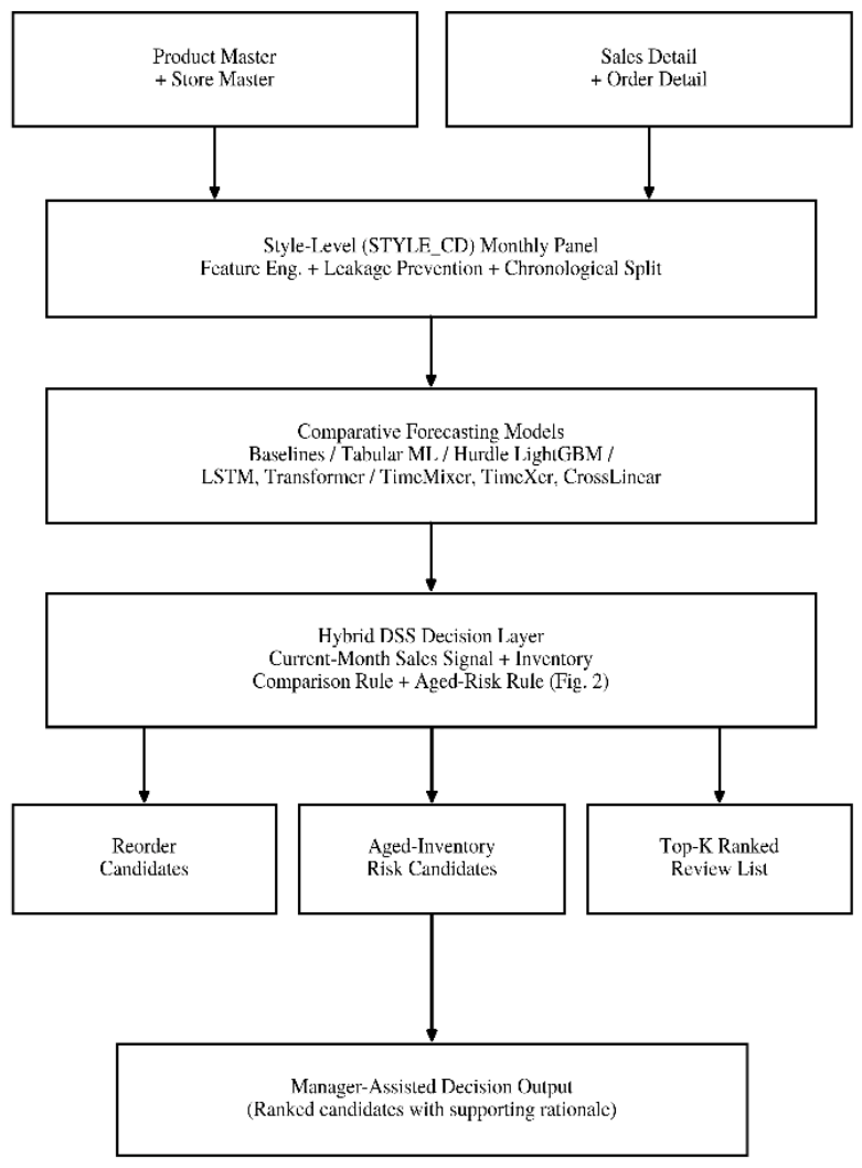
Figure 2.
Structure of the proposed Hybrid Decision Support System, combining the forecasting module (A) with the current-month sales signal (B), the inventory-comparison rule (C), Top-K ranking (D), and product-attribute interpretation (E).
Figure 2.
Structure of the proposed Hybrid Decision Support System, combining the forecasting module (A) with the current-month sales signal (B), the inventory-comparison rule (C), Top-K ranking (D), and product-attribute interpretation (E).
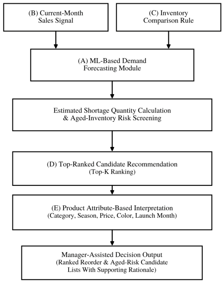
Figure 3.
WAPE comparison across benchmark models on the 2016 test period.
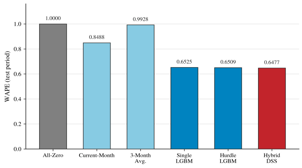
Figure 4.
Reorder precision, recall, and F1-score comparison across models.
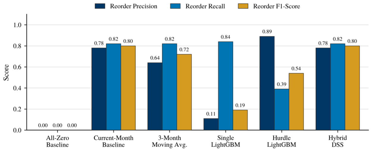
Figure 5.
Top-50 recommendation performance: Hit@50 and NDCG@50 across models.
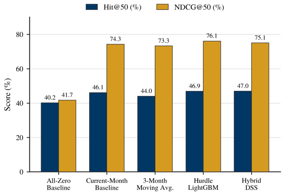
Figure 6.
(a) Training time and (b) inference time by model, measured on the 64,295-sample test set.
Figure 6.
(a) Training time and (b) inference time by model, measured on the 64,295-sample test set.
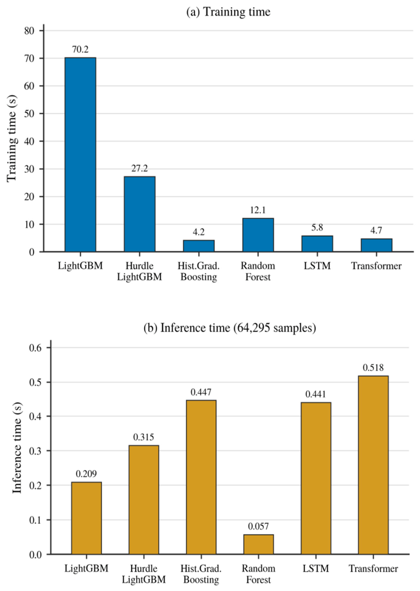
Figure 7.
Percentage change in key operational metrics under the DSS policy simulation scenario relative to current operation.
Figure 7.
Percentage change in key operational metrics under the DSS policy simulation scenario relative to current operation.
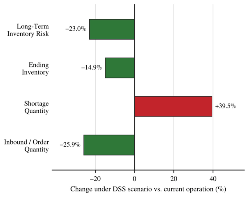

Table 1.
Composition of the research data.
| Data Type | Rows | Main Content | Role |
| Store Master | 1,347 | Store codes, attributes | Reference data |
| Product Master | 28,278 | Code, gender, season, category, price | Attribute interp. |
| Sales Detail | 4,130,603 | Sale date, code, quantity, amount | Target variable |
| Order Detail | 5,065,027 | Order/replenishment transactions | Inventory-flow rebuild |
| Detailed-item panel | 1,163,307 | Monthly agg. by item code | Color-size validation |
| Style-level panel | 263,260 | Monthly agg. by style code | Prediction / DSS analysis |
| Learning samples | 187,392 | 12-month history samples | Train/val/test split |
Table 2.
Feature groups used as model inputs.
| Feature Group | Key Variables | Interpretation |
| Current state | Current sales, stock, order status | Operating status at base month |
| Historical lags | Sales/orders at 1, 3, 6, 12 mo. prior | Past demand and replenishment flow |
| Rolling statistics | Recent sales mean, sum, std. dev. | Short-term trend and volatility |
| Zero-demand structure | Consecutive zero-sales months, recent signal | Sparse demand, long non-sales periods |
| Product attributes | Gender, season, category, base price | Fixed product characteristics |
| Life cycle | Months since launch, long-run flag | Product life-cycle stage |
Table 3.
Chronological training, validation, and test split.
| Partition | Period | Samples | Purpose |
| Training | 2012–2014 | 70,199 | Model training |
| Validation | 2015 | 52,898 | Model and policy selection |
| Test | 2016 | 64,295 | Final performance evaluation |
Table 4.
Comparative forecasting models and their roles.
| Category | Models | Role in the Study |
| Simple baselines | All-Zero; Current-Month Sales; 3-Mo. Moving Avg. | Lower-bound reference |
| Tabular ML | Random Forest; Hist. Gradient Boosting; LightGBM | Non-linear tabular learning |
| Sparse-demand | Hurdle LightGBM | Zero vs. positive demand split |
| Sequential DL | LSTM; Transformer | Temporal sequence learning |
| Recent time-series | TimeMixer; TimeXer; CrossLinear | Multiscale / exogenous / cross-corr. |
Table 5.
Prediction error and reorder decision performance by model (test period).
| Model | WAPE | MAE | Reorder Precision | Reorder Recall | Reorder F1 |
| All-Zero Baseline | 1.0000 | 4.6937 | 0.0000 | 0.0000 | 0.0000 |
| Current-Month Sales Baseline | 0.8488 | 3.9840 | 0.7797 | 0.8178 | 0.7983 |
| 3-Month Moving Average | 0.9928 | 4.6600 | 0.6401 | 0.8222 | 0.7198 |
| Single LightGBM | 0.6525 | 3.0625 | 0.1068 | 0.8356 | 0.1894 |
| Hurdle LightGBM | 0.6509 | 3.0550 | 0.8866 | 0.3822 | 0.5342 |
| Hybrid DSS (proposed) | 0.6477 | 3.0399 | 0.7797 | 0.8178 | 0.7983 |
Table 6.
Bootstrap-based test of pairwise WAPE differences.
| Comparison | Mean Diff. | 95% CI | Improv. Prob. |
| Hurdle LGBM - Current-Month Baseline | −0.1979 | [−0.2298, −0.1585] | 1.0000 |
| Hurdle LGBM - 3-Mo. Moving Avg. | −0.3443 | [−0.4132, −0.2852] | 1.0000 |
| Hurdle LGBM - Single LightGBM | −0.0019 | [−0.0115, 0.0084] | 0.6470 |
| Blended Forecast - Hurdle LGBM | −0.0022 | [−0.0040, −0.0006] | 0.9960 |
Table 7.
Comparative role of TimeMixer, TimeXer, and CrossLinear.
| Model | Focus | Best-Task Result | Interpretation |
| TimeMixer | Multiscale mixing | F1 = 0.7639 (reorder); WAPE = 0.3360 (aged-inv.) | Best reorder classification & long-horizon qty. |
| TimeXer | Exogenous vars. | Recall = 0.9611 (Prec. 0.4979, F1 0.6560) | Fewest missed candidates; broader list |
| CrossLinear | Cross-corr. embedding | WAPE = 0.6372 (shortage qty.) | Best shortage-quantity regression |
Table 8.
Top 5 recommendations for performance.
| Model | Hit@50 (%) | NDCG@50 (%) | Qty. Recall@50 |
| Current-Month Baseline | 46.12 | 74.33 | 0.8445 |
| Hybrid DSS (proposed) | 47.04 | 75.12 | 0.8445 |
| 3-Month Moving Average | 43.98 | 73.26 | 0.8067 |
| Hurdle LightGBM | 46.93 | 76.08 | 0.6630 |
| All-Zero Baseline | 40.24 | 41.74 | 0.2225 |
Table 9.
Detailed product-level (color-size) validation summary.
| Metric | Value | Interpretation |
| Validation observations | 228,053 | Rows at detailed-item level |
| Linked styles | 5,740 | Styles linked to candidates |
| Linked detailed items | 20,535 | Color-size execution items |
| Reorder precision | 0.7126 | True shortage share of proposals |
| Reorder recall | 0.5554 | True shortage items captured |
| Reorder F1 | 0.6243 | Precision-recall balance |
| 3-month demand WAPE | 0.6018 | Item-level quantity error |
| Qty. recall@50 | 65.78% | Shortage qty. captured, top 50 |
| Qty. recall@100 | 72.36% | Shortage qty. captured, top 100 |
Table 10.
Computational resource use by model (64,295 test samples).
| Model | Train (s) | Infer. (s) | Smpl/s | Mem. (MB) | GPU (MB) |
| LightGBM | 70.15 | 0.209 | 306,931 | 24.42 | 0.00 |
| Hurdle LightGBM | 27.22 | 0.315 | 204,278 | 0.46 | 0.00 |
| Hist. Grad. Boosting | 4.21 | 0.447 | 143,729 | 10.49 | 0.00 |
| Random Forest | 12.08 | 0.057 | 1,123,421 | 101.08 | 0.00 |
| LSTM | 5.77 | 0.441 | 145,895 | 815.57 | 106.67 |
| Transformer | 4.71 | 0.518 | 124,084 | 346.13 | 113.60 |
Table 11.
Key results of the policy simulation.
| Metric | Current Op. | DSS Scenario | Change Rate |
| Inbound / Order Qty. | 4,597,512 | 3,405,705 | −25.9% |
| Shortage Qty. | 303,570 | 423,414 | +39.5% |
| Ending Inventory | 7,190,501 | 6,118,538 | −14.9% |
| Long-Term Inventory Risk | 3,050,898 | 2,348,364 | −23.0% |
Disclaimer/Publisher’s Note: The statements, opinions and data contained in all publications are solely those of the individual author(s) and contributor(s) and not of MDPI and/or the editor(s). MDPI and/or the editor(s) disclaim responsibility for any injury to people or property resulting from any ideas, methods, instructions or products referred to in the content. |
© 2026 by the authors. Licensee MDPI, Basel, Switzerland. This article is an open access article distributed under the terms and conditions of the Creative Commons Attribution (CC BY) license.
Copyright: This open access article is published under a Creative Commons CC BY 4.0 license, which permit the free download, distribution, and reuse, provided that the author and preprint are cited in any reuse.