

Submitted:
05 September 2026
Posted:
08 September 2026
You are already at the latest version
Abstract
Heart rate variability (HRV) features provide compact representations of R-R interval (RRI) dynamics, but temporal information may be selectively lost during feature aggregation. This study investigated which aspects of temporal structure remain discriminable after RRI time series are compressed into HRV-based representations. Publicly available sinus rhythm and continuous atrial fibrillation (CAF) datasets were analyzed. For each RRI sequence, three temporal variants were generated: Forward, Reverse, and Shuffle. Three input representations were compared: raw RRI sequences, seven RRI-derived HRV features, and the same seven features supplemented with three temporal descriptors: Half Mean Difference, Linear Slope, and Difference Asymmetry (DAsym). Classification was evaluated across observation durations from 5 to 30 min using six machine-learning classifiers. Raw RRI classification was modest in sinus rhythm and approached chance level in CAF at durations of 10 min or longer. The 7-HRV representation substantially improved discrimination, particularly for Shuffle sequences, but Forward and Reverse remained more difficult to distinguish. Adding the three temporal features further improved classification, with accuracy reaching 0.803 in sinus rhythm and 0.923 in CAF. In CAF, DAsym showed the highest class-specific permutation importance for both Forward and Reverse at five of the six observation durations. Post-hoc analysis further showed that the magnitude of negative RRI changes exceeded that of positive changes in CAF (p<0.001). These findings indicate that feature aggregation does not uniformly eliminate temporal information: RRI-derived HRV features retain sensitivity to disruption of temporal organization but are comparatively insensitive to temporal direction. A small number of interpretable temporal descriptors may recover part of this lost directional information while preserving a compact representation. More broadly, compact physiological representations should be evaluated not only by how efficiently they can be transmitted, but also by what information they retain, what they omit, and whether the retained information is sufficient for the intended purpose.
Keywords:
heart rate variability
; R-R interval
; temporal structure
; feature aggregation
; physiological data transmission
1. Introduction
Heart rate variability (HRV) analysis provides a compact representation of beat-to-beat cardiovascular dynamics and is widely used to characterize autonomic regulation from R-R interval (RRI) time series [1,2]. Conventional HRV indices summarize different aspects of variability, including overall dispersion, short-term beat-to-beat fluctuation, and frequency-domain characteristics [1,2]. However, HRV indices exhibit substantial interindividual variability, and the physiological state at a particular time may not always be directly inferred from the absolute values of a limited number of HRV indices alone [2,3]. HRV indices are highly useful for statistical comparisons and for characterizing group-level differences across subjects, conditions, and recording periods [1,2,3].
An RRI time series provides a different form of information by preserving the temporal evolution of beat-to-beat intervals without compressing an observation interval into a small set of summary values [4,5]. For example, within a 5-min recording, the RRI time series allows direct observation of when intervals increased or decreased and how these changes developed over time. Conventional HRV indices compress this temporal behavior into a limited number of numerical descriptors and do not explicitly preserve the original beat-to-beat ordering within an analysis window [4]. HRV indices and RRI time series should not necessarily be regarded as competing representations; rather, they provide different views of the same physiological process.
Recent advances in wearable sensing, mobile health, wireless communication, and cloud-based monitoring have increased the use of continuously acquired electrocardiogram (ECG) and ECG-derived information outside conventional clinical settings [6,7]. Contemporary remote monitoring systems may transmit ECG waveforms to external servers for subsequent processing. Increasing processing capability at wearable or edge devices allows derived information to be extracted before transmission [6]. Reviews of wearable and remote ECG monitoring have highlighted the growing integration of ECG acquisition, local signal processing, wireless transmission, and cloud-based analysis [6,7].
In such systems, the level at which physiological information is transmitted represents an important design choice. The original ECG waveform contains the greatest signal-level detail. Derived representations can reduce the amount of data that must be transmitted. Accordingly, numerous studies have investigated ECG compression, local signal processing, and other strategies for reducing communication load and energy consumption in wearable and remote-monitoring systems [6,8,9,10]. More recently, feature-level or locally processed ECG transmission has been investigated as an alternative to continuous transmission of raw ECG waveforms [11,12,13]. These approaches are attractive for bandwidth- and energy-constrained wearable systems, but they raise a complementary question: what information becomes difficult to recover as physiological time series are progressively summarized?
This question is relevant to temporal information. Previous studies have demonstrated that heartbeat interval dynamics can exhibit temporal irreversibility and asymmetry, indicating that the direction and ordering of RRI changes may themselves contain physiological information [5,14,15,16]. Transmitting the complete RRI time series preserves the temporal ordering of beat-to-beat intervals but requires a larger data volume than transmitting only a small number of HRV indices. Conversely, HRV feature transmission provides a compact representation but may obscure information concerning temporal direction, local ordering, or gradual changes within the observation period. The issue is not whether conventional HRV indices are useful, but rather what temporal information they preserve and what becomes difficult to observe after an RRI time series is summarized.
One possible intermediate representation is to supplement conventional HRV indices with a small number of explicitly temporal features. Features describing early-to-late changes, overall trends, or directional asymmetry may retain information about temporal organization without requiring transmission of the complete RRI time series. Such a representation could potentially preserve some of the temporal information contained in the original sequence and maintain a compact feature set.
The extent to which temporal information is retained may depend on the underlying cardiac rhythm. Sinus rhythm contains organized beat-to-beat modulation arising from physiological regulatory processes. CAF exhibits markedly different RRI dynamics [17,18]. Importantly, irregular ventricular timing during AF does not necessarily imply complete temporal randomness, because serial dependencies in successive RRIs have been reported [18].
To investigate these questions, three temporally distinct versions of each RRI time series were constructed: the original Forward series, a Reverse series preserving the same RRI values with inverted temporal direction, and a Shuffle series in which the same values were randomly reordered. Three input representations were then compared: (i) the raw RRI time series, (ii) seven RRI-derived HRV features, and (iii) the same seven RRI-derived HRV features supplemented with three temporal features: Half Mean Difference (HMD), Linear Slope (LSlope), and Difference Asymmetry (DAsym). Specifically, we examined (i) whether Forward, Reverse, and Shuffle series could be discriminated directly from the raw RRI time series; (ii) whether these temporal differences remained discriminable after compression into RRI-derived HRV features; and (iii) whether adding a small number of temporal features improved discrimination of temporal direction and organization. By comparing these three representations in sinus rhythm and CAF, the present study aimed to clarify how temporal information is altered by HRV feature aggregation and whether a small number of additional temporal descriptors can retain information that is otherwise difficult to access from RRI-derived HRV features alone.
2. Materials and Methods
2.1. Study Design and Datasets
Publicly available datasets from PhysioNet were used to construct the sinus rhythm and AF cohorts [19]. The sinus rhythm cohort comprised the Fantasia Database [20,21], the Normal Sinus Rhythm RRI Database [19,22], and RRI time series from healthy subjects [23,24]. The AF cohort comprised the MIT-BIH AF Database [25,26], the Long-Term AF Database [27,28], and the SHDB-AF database [29,30]. Participant characteristics, the number of records included from each database, and the corresponding Mean RRI and SDRR (standard deviation of R-R intervals) values are summarized in Table 1.
2.2. RRI Preprocessing and Duration Selection
For all datasets, RRIs were defined from consecutive beat annotations as
RRIi =Ri +1−Ri
Because each RRI becomes fully defined only when the later R peak, Ri +1, occurs, each interval was assigned to the time of that later beat. This convention aligns the RRI value with the time at which it becomes available and avoids assigning an interval to an earlier time at which its duration has not yet been determined. This timestamp convention was maintained during subsequent interpolation and resampling so that the reconstructed RRI time series remained aligned with the actual time at which each interval was completed.
For the sinus rhythm datasets, RRIs associated with atrial premature beats (A) or ventricular premature beats (V), RRIs shorter than 400 ms or longer than 1600 ms, and non-finite values were excluded. The original timestamps of the remaining RRIs were preserved. The cleaned RRI sequence was divided at gaps exceeding 5 s, and the first continuous segment lasting at least 30 min was identified. The first 30 min of this segment was selected for analysis. The irregularly sampled RRI sequence was then interpolated using piecewise cubic Hermite interpolating polynomial (PCHIP) interpolation and resampled at 2 Hz, yielding 3600 samples.
After resampling of the sinus rhythm data, sequential spike correction was applied. For each sample, the mean of the previous three corrected RRI values was calculated. If the current value differed from this mean by more than 30%, it was replaced by the mean of the previous three corrected values. Corrected values were subsequently used when evaluating the following samples.
For the AF datasets, rhythm annotations were used to identify continuous AF episodes. Only recordings containing at least 30 min of uninterrupted AF were included. RRIs were calculated only from consecutive QRS complexes for which both beats were contained within the same AF episode; RRIs crossing the onset or termination of AF were excluded. The first usable 30-min interval beginning from the first AF-contained RRI within an eligible continuous AF episode was selected.
In contrast to the sinus rhythm preprocessing, no fixed upper or lower RRI threshold was applied to the AF data. No clean-segment criterion or maximum-gap rejection was used, and no spike correction was performed after resampling. Only non-finite or non-positive RRIs were excluded. These choices were made to preserve the large beat-to-beat RRI variability characteristic of AF without treating such variability as artifactual. The selected AF RRI sequence was interpolated using PCHIP and resampled at 2 Hz, yielding 3600 samples over 30 min. The first RRI point at or beyond the final target time was retained only as a right-side support point for PCHIP interpolation. For both rhythm groups, six observation durations were evaluated: 5, 10, 15, 20, 25, and 30 min.
2.3. Generation of Forward, Reverse, and Shuffle Sequences
To evaluate what aspects of temporal information are retained in HRV representations, three versions of each RRI sequence were constructed. The original Forward sequence retained the observed temporal organization. The Reverse sequence preserved exactly the same RRI values and reversed their temporal direction, allowing sensitivity to directional information to be assessed. The Shuffle sequence preserved the same set of RRI values but randomized their order, thereby disrupting local temporal organization. By comparing discrimination among these three sequence types, we aimed to distinguish sensitivity to temporal direction from sensitivity to temporal organization more generally.
For both sinus rhythm and AF, six observation durations were evaluated: 5, 10, 15, 20, 25, and 30 min. For each duration, the corresponding initial portion of the preprocessed 30-min RRI sequence was extracted (Figure 1).
From each extracted RRI sequence, three variants were generated: Forward, Reverse, and Shuffle. The Forward sequence was defined as the original RRI sequence in its observed temporal order. The Reverse sequence was generated by reversing the order of the entire RRI sequence. The Shuffle sequence was generated by randomly permuting all RRI values within the selected interval, thereby preserving the set of RRI values and disrupting their original temporal ordering.
The Shuffle series was generated by randomly permuting the RRI values using NumPy’s default random number generator. To ensure reproducibility, a subject- and duration-specific random seed was derived from a fixed base seed (20260818) using Secure Hash Algorithm 256-bit, ensuring that the same subject and duration always produced the same shuffled series.
Let the selected RRI sequence be
x=[x1, x2 ,…, xN]
The Forward sequence was defined as
and the Reverse sequence as
xF=[x1, x2,…, xN]
xR=[xN, xN−1, …, x1]
The Shuffle sequence was defined as
where π denotes a random permutation of the indices 1, …, N.
xS=[xπ(1), xπ(2), …, xπ(N)]
The three variants contained identical RRI values within each subject and duration; only their temporal organization differed. All three variants derived from the same subject were kept within the same training or test partition to prevent subject-level information leakage.
2.4. Feature Representations
To examine how temporal information is retained or lost through feature aggregation, three input representations were compared: (i) Raw RRI, (ii) 7-HRV, and (iii) 7-HRV + 3 temporal features. The same Forward, Reverse, and Shuffle sequences were used to construct each representation.
2.4.1. Raw RRI Representation
For the Raw RRI representation, the resampled RRI values themselves were used directly as classifier inputs. Because all RRI sequences had been resampled at 2 Hz, the number of input values depended on the observation duration: 600, 1200, 1800, 2400, 3000, and 3600 samples for 5, 10, 15, 20, 25, and 30 min, respectively.
This representation retained the full temporal ordering of the RRI sequence without feature aggregation.
2.4.2. 7-HRV Representation
For the 7-HRV representation, the analysis was designed under the assumption that physiological information would be transmitted sequentially in 5-min units. Each Forward, Reverse, or Shuffle RRI sequence was divided chronologically into consecutive non-overlapping 5-min windows. Drawing on commonly used time- and frequency-domain HRV indices described in the ESC/NASPE Task Force recommendations [1], the seven-feature representation was based on a compact feature set previously used for feature-level physiological data transmission [13]. The feature set comprised SDNN, RMSSD, pNN50, low-frequency (LF) power, high-frequency (HF) power, the ratio of low-frequency to high-frequency power (LF/HF), and Mean heart rate (HR). In the present study, Mean RRI was used instead of Mean HR to maintain the representation directly in the RRI domain. Because Mean HR is uniquely determined from Mean RRI, this substitution does not add or remove an independent descriptor. In addition, SDRR was used instead of SDNN because the present analysis included RRI series from continuous atrial fibrillation and was not restricted to normal-to-normal intervals. Seven RRI-derived HRV features—Mean RRI, SDRR, RMSSD, pNN50, LF, HF, and LF/HF—were calculated separately for each window.
Frequency-domain features were estimated using Welch’s method with a symmetric Hann window, 240-sample segments, and 50% overlap. LF power was calculated over 0.04≤f<0.15 Hz and HF power over 0.15≤f≤0.40 Hz, and LF/HF was calculated as the ratio of LF to HF power. All seven HRV indices were calculated from the RRI series resampled at 2 Hz to ensure that the Raw RRI and HRV representations were derived from the same underlying time-series representation. Accordingly, RMSSD and pNN50 were calculated from successive samples of the 2-Hz RRI series and not directly from successive beat-to-beat intervals. The seven HRV indices obtained from each 5-min window were treated as a 7-dimensional feature vector. For observation durations longer than 5 min, the feature vectors from successive windows were concatenated in chronological order to form a single input vector for machine-learning classification. For example, the 10-min representation was constructed as
where h=[Mean RRI, SDRR, RMSSD, pNN50, LF,HF, LF/HF].
x10=[h0−5, h5−10]
Accordingly, the input dimensions for observation durations of 5, 10, 15, 20, 25, and 30 min were 7, 14, 21, 28, 35, and 42 features, respectively. This construction represents a transmission scenario in which a compact 7-dimensional HRV feature vector is transmitted every 5 min and sequentially accumulated at the receiving side; the complete RRI time series is not transmitted. Consequently, the HRV representation retained coarse temporal progression across successive 5-min windows and substantially compressed the temporal information contained in the RRI series within each window.
2.4.3. 7-HRV + 3 Temporal-Feature Representation
To explicitly represent temporal characteristics that may not be fully captured by the seven RRI-derived HRV features, three additional temporal features were calculated from the entire RRI sequence for each observation duration: (a) HMD, (b) LSlope, and (c) DAsym. These features were appended to the chronologically concatenated 7-HRV feature vector. The three temporal features were calculated once for the complete RRI sequence at each observation duration and were not calculated separately for individual windows.
(a) HMD
The sequence was divided into first and second halves, and the difference between their mean RRI values was calculated as
where N1=N/2 and N2=N−N1.
Positive values indicate that the mean RRI was larger in the first half than in the second half; negative values indicate the opposite. This feature represents a coarse temporal difference between the earlier and later portions of the sequence. The implementation directly computes the first-half mean minus the second-half mean.
(b) LSlope
The overall linear trend of the RRI sequence was quantified using the least-squares regression slope,
where ti represents the sequential sample index, is its mean, and is the mean RRI.
Positive values indicate an overall increase in RRI across the sequence; negative values indicate an overall decrease.
(c) DAsym
Successive RRI differences were first calculated as
Δxi = xi + 1 − xi
Positive and negative differences were then separated. DAsym was defined as
If no positive or negative differences were present, the corresponding mean was set to zero. DAsym quantifies the imbalance between the average magnitude of RRI increases and decreases. Positive values indicate larger average increases; negative values indicate larger average decreases.
2.5. Machine-Learning Classification
For each rhythm group, observation duration, and input representation, three-class classification was performed to distinguish the Forward, Reverse, and Shuffle sequences. Six classifiers were evaluated: Extreme Gradient Boosting (XGBoost), logistic regression (LGR), quadratic discriminant analysis (QDA), Gaussian naive Bayes (NB), k-nearest neighbors (KNN), and linear discriminant analysis (LDA). The classifier settings are summarized in Table 2.
Classification was performed using 10 repeated subject-wise training/test splits. The repeated splitting procedure was defined as follows:
- Within each split, all Forward, Reverse, and Shuffle sequences derived from the same subject were assigned to the same partition to prevent subject-level information leakage.
- Individual subjects could appear in the test set in multiple repeated splits. To preserve the dependency associated with repeated test-set appearances of the same subject, a subject-blocked permutation test was used.
- The same split definitions were used across the three input representations.
- Complete subject-wise training/test assignments for all 10 splits are provided in Supplementary Data S1 for sinus rhythm and Supplementary Data S2 for CAF.
Fixed classifier settings were used throughout the analysis, and no validation-set or test-set hyperparameter tuning was performed. For logistic regression and KNN, predictor variables were standardized using StandardScaler fitted only to the training data and subsequently applied to the corresponding test data.
Each classifier was evaluated independently for every observation duration and input representation within each rhythm group. For summary reporting, the classifier with the highest mean Macro-F1 across the 10 subject-wise splits was regarded as the best-performing classifier for that duration and representation.
All analyses and evaluations were implemented in Python 3.12.7 (64-bit). Numerical computation and data handling were performed using NumPy and pandas. Machine-learning models were implemented using scikit-learn for LGR, QDA, NB, KNN, and LDA, and XGBoost for XGB.
2.6. Performance Evaluation
Classification performance was evaluated separately for each rhythm group, observation duration, input representation, and classifier. The primary performance measures were accuracy and Macro-F1 score.
Accuracy was defined as
where is the number of correctly classified samples and is the total number of samples.
For each class , precision and recall were calculated as
where TPc, FPc, and FNc denote the numbers of true-positive, false-positive, and false-negative classifications for class c, respectively.
The class-specific F1 score was defined as
Macro-F1 was calculated as the unweighted mean of the F1 scores for the three classes, Forward, Reverse, and Shuffle:
Each class contributed equally to the overall Macro-F1 score.
For each classifier, these performance measures were calculated independently for each of the 10 subject-wise test splits and are reported as the mean ± standard deviation (SD) across splits. Class-specific F1 scores were retained to assess differences in classification performance among Forward, Reverse, and Shuffle.
Confusion matrices were constructed for each test split, with rows representing the true class and columns representing the predicted class. For summary reporting, confusion-matrix counts for the best-performing classifier were pooled across the 10 subject-wise splits, and row-wise classification rates were calculated from the pooled counts:
where Cij denotes the number of samples belonging to true class i that were classified as class j.
Macro-averaged receiver operating characteristic area under the curve (ROC-AUC) was additionally calculated using a one-versus-rest approach:
where AUCc is the ROC-AUC obtained by treating class c as the positive class and the remaining two classes as the negative class. Macro ROC-AUC was treated as a supplementary performance measure.
2.7. Subject-Blocked Permutation Test
フォームの始まり
フォームの終わり
To assess whether the observed classification accuracy exceeded that expected under random correspondence between the predicted and true class labels, a subject-blocked permutation test was performed separately for each observation duration and classifier. Because the classification task comprised three equally represented classes—Forward, Reverse, and Shuffle—the nominal chance level was 1/3. The observed test statistic was defined as the mean held-out test accuracy across the 10 subject-wise splits:
where As denotes the classification accuracy for split , and S=10.
For the permutation procedure, the predictions generated by the fitted classifiers were kept fixed, and only the correspondence among the true Forward, Reverse, and Shuffle labels was permuted. Because the same subject could appear in the test set of multiple repeated splits, the permutation procedure was blocked by subject. In each permutation iteration, one random permutation of the three class labels was independently generated for each subject. The same subject-specific label mapping was then reused in every split in which that subject appeared, thereby preserving the dependency associated with repeated test-set appearances of the same subject.
For each permutation b, the mean accuracy across the 10 splits was calculated as
where As,b is the accuracy for split after subject-blocked permutation of the true labels. A total of B=10,000 permutations were performed.
The one-sided permutation p-value was calculated as
where I (⋅) is the indicator function. This procedure tested whether the observed mean held-out accuracy was greater than expected under the null distribution generated by subject-blocked random reassignment of the class labels. The classifiers were not retrained during the permutation procedure.
2.8. Permutation Importance Analysis
Permutation importance was used as a post-hoc analysis to quantify the contribution of individual input features to classification performance. The analysis was performed exclusively on the held-out test data and was not used for model selection or hyperparameter tuning.
For each feature j, its values were randomly permuted across test samples, with all other features left unchanged. The fitted classifier was then applied to the permuted test data. Overall permutation importance was defined as the decrease in Macro-F1 relative to the unpermuted test data:
where is the Macro-F1 obtained using the original test data and is the Macro-F1 obtained after permutation of feature j.
Each feature was permuted 30 times, and the mean decrease in Macro-F1 across the 30 repetitions was used as its permutation importance. Positive values indicated that disruption of the feature reduced classification performance, indicating that the feature contributed positively to prediction. Values near zero indicated little measurable contribution. Negative values indicated that permutation occasionally improved classification performance and were interpreted as unstable or negligible contributions.
In addition to overall permutation importance, class-specific permutation importance was calculated separately for Forward, Reverse, and Shuffle. For each target class c, the corresponding class-specific F1 score was used as the performance measure. Class-specific permutation importance for feature j was defined as
where is the F1 score for class obtained from the original test data and is the corresponding F1 score after permutation of feature j. This analysis was used to identify features that contributed specifically to the recognition of each sequence type.
For HRV representations containing multiple consecutive 5-min windows, permutation importance was initially retained separately for each feature position, such as W01_RMSSD and W02_RMSSD. For summary analyses, importance values for the same HRV index were subsequently averaged across window positions and subject-wise splits for each observation duration and classifier. Class-specific permutation importance was summarized in the same manner.
For the 7-HRV + 3 temporal-feature representation, the three temporal features were retained individually because each temporal feature was calculated once from the complete RRI sequence for the corresponding observation duration rather than separately within each 5-min window.
3. Results
3.1. Validation (i): Classification Using Raw RRI Sequences
Table 3 summarizes the classification performance obtained using the raw RRI representation in sinus rhythm and CAF. In sinus rhythm, mean accuracy ranged from 0.479 to 0.548, and Macro-F1 ranged from 0.480 to 0.547 across observation durations. The highest accuracy was obtained at 10 min using NB (accuracy, 0.548±0.100; Macro-F1, 0.547±0.100; Macro-AUC, 0.689±0.099). Macro-AUC ranged from 0.656 to 0.718 and reached its highest value at 30 min (0.718±0.058).
In CAF, the highest accuracy was observed at 5 min using NB (accuracy, 0.438±0.099; Macro-F1, 0.428±0.097; Macro-AUC, 0.602±0.088). From 10 to 30 min, mean accuracy ranged from 0.331 to 0.369, Macro-F1 from 0.327 to 0.365, and Macro-AUC from 0.488 to 0.543.
Table 4 shows the confusion matrices and subject-blocked permutation-test results for the best-performing classifier at each observation duration. In sinus rhythm, classification accuracy was significant at all observation durations (p<0.001). At 30 min, the correct classification rates were 0.555 for Forward, 0.555 for Reverse, and 0.482 for Shuffle. Forward sequences were classified as Reverse in 0.336 of cases, and Reverse sequences were classified as Forward in 0.327 of cases. The correct classification rate for Shuffle was 0.355, 0.618, 0.527, 0.445, 0.400, and 0.482 at 5, 10, 15, 20, 25, and 30 min, respectively.
In CAF, classification accuracy was significant at 5 min (p<0.001), with correct classification rates of 0.546 for Forward, 0.500 for Reverse, and 0.269 for Shuffle. At 10, 15, 20, 25, and 30 min, the permutation-test p-values were 0.447, 0.265, 0.548, 0.135, and 0.188, respectively. At 20 min, the correct classification rates were 0.323 for Forward, 0.338 for Reverse, and 0.331 for Shuffle.
3.2. Validation (ii): Classification Using the 7-HRV Representation
Table 5 summarizes the classification performance obtained using the 7-HRV representation in sinus rhythm and CAF. In sinus rhythm, mean accuracy ranged from 0.661 to 0.755, and Macro-F1 ranged from 0.657 to 0.753 across observation durations. The highest accuracy was observed at 15 min using XGB (accuracy, 0.755 ± 0.086; Macro-F1, 0.753 ± 0.086; Macro-AUC, 0.891 ± 0.055). Macro-AUC ranged from 0.830 to 0.891.
In CAF, mean accuracy ranged from 0.656 to 0.721, and Macro-F1 ranged from 0.634 to 0.721. The highest accuracy was obtained at 25 min using QDA (accuracy, 0.721 ± 0.117; Macro-F1, 0.721 ± 0.118; Macro-AUC, 0.860 ± 0.055). At 30 min, the accuracy was 0.718 ± 0.062, the Macro-F1 was 0.720 ± 0.061, and the Macro-AUC was 0.834 ± 0.046.
Table 6 shows the corresponding confusion matrices and subject-blocked permutation-test results. In sinus rhythm, classification accuracy was significant at all observation durations (p<0.001). Shuffle sequences were classified with near-perfect accuracy across all durations, with correct classification rates of 1.000 at 5, 10, 15, 20, and 30 min and 0.982 at 25 min. Forward and Reverse were substantially more difficult to distinguish. The correct classification rate for Forward ranged from 0.473 to 0.627. The corresponding range for Reverse was 0.509 to 0.655. At 5 min, the correct classification rates were 0.473 for Forward and 0.509 for Reverse. Shuffle was classified correctly in 1.000 of pooled test appearances.
In CAF, classification accuracy was significant at all observation durations (p<0.001). The correct classification rate for Shuffle ranged from 0.954 to 0.992. For Forward, the correct classification rate ranged from 0.546 to 0.600. For Reverse, it ranged from 0.438 to 0.615. At 5 min, Forward and Reverse showed marked mutual confusion: 0.546 of Forward sequences were correctly classified; 0.438 were classified as Reverse. For Reverse sequences, 0.438 were correctly classified and 0.546 were classified as Forward. At 30 min, the correct classification rates were 0.577 for Forward and 0.615 for Reverse.
Figure 3 shows the three highest positive class-wise permutation importance values for each observation duration and target class. Non-positive values were omitted from the figure.
In sinus rhythm, Forward classification generally showed small permutation importance values. At 10 min, Mean RRI, SDRR, and RMSSD showed the highest positive values (0.085, 0.060, and 0.038, respectively). At 25 min, SDRR showed the largest Forward importance (0.042), followed by Mean RRI (0.015) and LF/HF (0.011). For Reverse classification, the largest values were modest; at 10 min, Mean RRI, SDRR, and RMSSD showed importance values of 0.089, 0.056, and 0.039, respectively. For Shuffle classification, larger contributions were observed at 5 min, where pNN50 and RMSSD showed importance values of 0.218 and 0.156, respectively. At longer durations, Shuffle importance values were generally smaller.
In CAF, Forward and Reverse classification showed consistently larger positive importance values than those observed in sinus rhythm. For Forward classification, RMSSD and SDRR showed the largest values at 5 min (0.169 and 0.116, respectively). At 10–30 min, Mean RRI, RMSSD, and SDRR were generally among the dominant features. For Reverse classification, RMSSD, Mean RRI, and SDRR similarly showed the largest importance values across most durations. For Shuffle classification, substantially larger importance values were observed. At 5 min, RMSSD and SDRR showed importance values of 0.799 and 0.685, respectively. At 10 min, Mean RRI, RMSSD, and SDRR showed values of 0.626, 0.622, and 0.563, respectively; at 15 min, the corresponding dominant values were 0.639 for Mean RRI, 0.574 for SDRR, and 0.570 for RMSSD. Similar patterns were observed at 25 and 30 min, with Mean RRI, SDRR, and RMSSD remaining the dominant contributors to Shuffle classification.
3.3. Validation (iii): Classification Using the 7-HRV + Temporal Representation
Table 7 summarizes the classification performance obtained using the 7-HRV + temporal representation in sinus rhythm and CAF. In sinus rhythm, mean accuracy ranged from 0.715 to 0.803, and Macro-F1 ranged from 0.715 to 0.803 across observation durations. The highest accuracy was observed at 25 min using KNN (accuracy, 0.803 ± 0.126; Macro-F1, 0.803 ± 0.126; Macro-AUC, 0.900 ± 0.062). The highest Macro-AUC was observed at 10 min using KNN (0.901 ± 0.052). At 5 min, QDA achieved an accuracy of 0.752 ± 0.083. At 30 min, KNN achieved an accuracy of 0.748 ± 0.043.
In CAF, mean accuracy ranged from 0.854 to 0.923, and Macro-F1 ranged from 0.854 to 0.923. The highest accuracy was observed at 20 min using XGB (accuracy, 0.923 ± 0.051; Macro-F1, 0.923 ± 0.052; Macro-AUC, 0.976 ± 0.021). At 25 min, XGB achieved an accuracy of 0.903 ± 0.048, a Macro-F1 of 0.903 ± 0.048, and a Macro-AUC of 0.975 ± 0.024. At 30 min, the accuracy remained high at 0.892 ± 0.063, with a Macro-F1 of 0.892 ± 0.063 and a Macro-AUC of 0.971 ± 0.024.
Table 8 shows the corresponding confusion matrices and subject-blocked permutation-test results. In sinus rhythm, classification accuracy was significant at all observation durations (p<0.001). The correct classification rate for Shuffle remained nearly perfect, ranging from 0.991 to 1.000. Forward and Reverse were more difficult to distinguish. The correct classification rate ranged from 0.582 to 0.709 for Forward and from 0.573 to 0.709 for Reverse. At 5 min, the correct classification rates were 0.627 for both Forward and Reverse. Shuffle was classified correctly in 1.000 of pooled test appearances. At 10 min, the corresponding rates were 0.691, 0.664, and 1.000, respectively. The highest correct classification rates for both Forward and Reverse were observed at 25 min, at 0.709. Shuffle was classified correctly in 0.991 of pooled test appearances.
In CAF, classification accuracy was significant at all observation durations (p<0.001). The correct classification rate ranged from 0.785 to 0.908 for Forward, from 0.762 to 0.892 for Reverse, and from 0.915 to 0.992 for Shuffle. At 20 min, the correct classification rates were 0.908 for Forward, 0.877 for Reverse, and 0.985 for Shuffle. At 25 min, the corresponding rates were 0.900, 0.892, and 0.915, respectively. At 30 min, Forward and Reverse were both classified correctly in 0.854 of pooled test appearances. Shuffle was classified correctly in 0.969.
Figure 4 shows the three highest class-wise permutation importance values for each observation duration and target class. In sinus rhythm, temporal features contributed prominently to Forward and Reverse classification. For Forward classification, DAsym showed the highest importance at 10, 15, 20, and 25 min, with values of 0.108, 0.063, 0.045, and 0.051, respectively. At 5 min, RMSSD showed the highest importance (0.164), followed by HMD (0.157) and LF/HF (0.092). At 30 min, HMD showed the highest importance (0.014), followed by DAsym (0.012) and SDRR (0.012). For Reverse classification, DAsym showed the highest importance at 10, 15, 20, and 25 min, with values of 0.098, 0.069, 0.042, and 0.066, respectively. At 5 and 30 min, HMD showed the highest importance, with values of 0.153 and 0.017, respectively. Shuffle classification was dominated by conventional HRV indices. At 5 min, RMSSD, SDRR, and LF/HF showed importance values of 0.612, 0.323, and 0.321, respectively. pNN50 showed the highest importance at 10–30 min.
In CAF, DAsym showed a dominant contribution to Forward and Reverse classification across most observation durations. For Forward classification, DAsym was the highest-ranked feature at 5, 15, 20, 25, and 30 min, with importance values of 0.298, 0.402, 0.446, 0.430, and 0.386, respectively. At 10 min, HMD and Mean RRI showed equally high importance values of 0.781, followed by DAsym at 0.295. For Reverse classification, DAsym was the highest-ranked feature at 5, 15, 20, 25, and 30 min, with corresponding values of 0.316, 0.374, 0.400, 0.444, and 0.390. At 10 min, HMD and Mean RRI again showed equally high importance values of 0.767, followed by DAsym at 0.291. For Shuffle classification, RMSSD and SDRR showed the highest importance values at 5 min (0.768 and 0.658, respectively) and remained the two highest-ranked features at 10 min (0.597 and 0.536, respectively). At 15 min, LSlope showed the highest importance (0.053). DAsym showed the highest importance at 20, 25, and 30 min, with values of 0.049, 0.048, and 0.055, respectively.
3.4. Post-Hoc Analysis of DAsym in CAF
Because DAsym showed the highest class-specific permutation importance for Forward and Reverse classification in CAF, a post-hoc analysis was performed to examine the directional imbalance of successive RRI changes in the original Forward records. Across the 122 CAF records, the mean positive RRI change was 100 ± 28 ms, and the mean absolute negative RRI change was 111 ± 45 ms. The magnitude of negative RRI changes was significantly greater than that of positive RRI changes (Wilcoxon signed-rank test, W=241, p<0.001). The corresponding mean DAsym, defined as the mean positive change minus the mean absolute negative change, was −11 ms. Figure 5 shows the distributions of the positive and absolute negative RRI change magnitudes.
Figure 6 summarizes the mean Macro-F1 scores across the three input representations and observation durations. In both rhythm groups, the 7-HRV representation showed higher Macro-F1 than the Raw RRI representation across all observation durations. Addition of the three temporal features further increased Macro-F1, with a more pronounced improvement in CAF.
4. Discussion
4.1. Principal Findings
The present study examined which aspects of temporal information contained in RRI time series remained discriminable after the original sequence was represented by RRI-derived HRV features, and whether a small number of additional temporal descriptors could improve access to information that was difficult to discriminate from these features alone. Three principal findings emerged. First, classification based directly on raw RRI sequences was modest in sinus rhythm and approached chance level in CAF at observation durations of 10 min or longer. The relatively low performance of the Raw RRI representation should not be interpreted as evidence that the original RRI series lacked temporal information. Raw RRI inputs were substantially higher-dimensional than the feature-based representations, and extracting discriminative temporal structure from such inputs may have been more difficult under the present sample size and classifier settings.
Second, the 7-HRV representation substantially improved discrimination of Shuffle sequences, whereas Forward and Reverse sequences remained more difficult to distinguish. Third, adding three temporal features further improved Forward–Reverse discrimination, with a marked improvement in CAF, where DAsym showed the highest class-specific permutation importance for both Forward and Reverse at five of the six observation durations. These findings indicate that different representations of the same RRI data retain different aspects of temporal information: RRI-derived HRV features were highly sensitive to disruption of temporal organization, whereas explicit temporal descriptors were more informative for temporal direction.
4.2. Different Effects of Temporal Reversal and Shuffling
A notable finding was the contrasting behavior of the Reverse and Shuffle transformations. Both transformations preserved exactly the same set of RRI values as the Forward sequence, but altered their temporal ordering in fundamentally different ways. Temporal reversal inverted the direction of the sequence and largely preserved its local adjacency structure. Shuffling disrupted the original adjacency relationships among RRI values. Consequently, the 7-HRV representation distinguished Shuffle sequences with very high accuracy but showed substantially greater difficulty separating Forward from Reverse. This contrast indicates that the RRI-derived HRV features were sensitive to disruption of local temporal organization but comparatively insensitive to temporal direction. A temporally altered sequence may remain difficult to distinguish when the altered property is not explicitly represented by the selected features. Conversely, disruption of local adjacency, as in the Shuffle condition, can substantially change the resulting HRV representation and make the altered sequence readily distinguishable.
4.3. Why RRI-Derived HRV Features are Relatively Insensitive to Temporal Direction
The difficulty in distinguishing Forward from Reverse sequences using the RRI-derived HRV features can be understood from their mathematical properties. Time reversal preserves the set of RRI values and leaves distribution-based measures such as Mean RRI and SDRR unchanged when calculated over the same interval. Similarly, for a Forward sequence, successive differences are defined as Δxi = xi+1−xi. Under exact temporal reversal, the corresponding differences appear in the opposite order with reversed sign. Consequently, quantities based on |Δxi |or (Δxi)2, such as pNN50 and RMSSD, are invariant to temporal reversal when calculated over the same sequence.
A similar principle applies to frequency-domain HRV measures. Temporal reversal preserves the power spectrum of a finite sequence; LF power, HF power, and the LF/HF ratio do not inherently encode whether a temporal pattern occurred in the forward or reverse direction. The Forward–Reverse results were consistent with these mathematical properties.
Within an individual 5-min window, the 7-HRV representation had limited ability to distinguish a sequence from its time-reversed counterpart, indicating that it could not reliably identify the direction in which RRI changes unfolded over time. The representation retained information about the magnitude and local temporal organization of variability but largely lost information about the direction of temporal evolution within the window.
Conceptually, this is analogous to playing a recorded process backward. The same set of observations remains present, but the direction in which the process unfolded is reversed. For example, a gradual increase in RRI becomes a gradual decrease after temporal reversal, even though the constituent RRI values are unchanged. Conventional HRV features can preserve the magnitude of variability in such a sequence while providing limited information about whether that variability unfolded in one temporal direction or the other.
For observation periods comprising multiple windows, the resulting HRV vectors were concatenated chronologically as
where denotes the seven-dimensional HRV feature vector obtained from the -th window. After reversal of the complete RRI sequence, the corresponding representation became
though temporal direction within each individual 5-min window was largely lost after compression into the 7-HRV representation, the chronological ordering of successive 5-min HRV vectors was retained for observation durations longer than 5 min. Reversal of the complete sequence reversed the order of these feature vectors, preserving a coarse form of temporal progression that remained available for Forward–Reverse discrimination. Shuffling disrupted local adjacency and substantially altered difference- and frequency-based features, providing a mechanistic explanation for the much higher discriminability of Shuffle sequences.
A methodological consideration is that Forward–Reverse invariance may depend on the implementation of the spectral estimator. In the present study, LF, HF, and LF/HF were estimated using Welch’s method with 240-sample segments, 50% overlap, and a symmetric Hann window. For each 5-min analysis window containing 600 samples, this configuration covered the complete sequence with four overlapping segments and treated the two sequence boundaries symmetrically under temporal reversal. The spectral estimation procedure was designed to minimize implementation-related Forward–Reverse differences arising from unequal boundary coverage or asymmetric window weighting.
4.4. Contribution of DAsym
DAsym was introduced to explicitly represent directional information that was largely absent from the RRI-derived HRV features. It was defined from successive sample-to-sample changes in the resampled RRI series as the difference between the mean magnitude of positive changes and that of negative changes. Unlike RMSSD and pNN50, which treat increases and decreases symmetrically, DAsym retains the imbalance between the two directions of change. Under exact temporal reversal, each successive RRI difference changes sign and the positive and negative difference sets are exchanged. This gives
making DAsym directly sensitive to temporal direction. Directional asymmetry and temporal irreversibility in heartbeat interval dynamics have previously been demonstrated using several related approaches [5,14,15,16].
This property was particularly relevant in CAF. In the original CAF sequences, the mean magnitude of RRI decreases exceeded that of RRI increases, producing negative DAsym values. Temporal reversal exchanged the positive and negative changes, shifting DAsym to the opposite sign. This directional separation provides a plausible explanation for the marked improvement in Forward–Reverse discrimination after the temporal features were added. Consistent with this interpretation, DAsym showed the highest class-specific permutation importance for both Forward and Reverse classification in CAF at five of the six observation durations and remained among the three highest-ranked features at 10 min. In sinus rhythm, its contribution was smaller and less consistent, indicating that this directional asymmetry provided less discriminative information in the sinus rhythm data.
The strong contribution of DAsym should therefore be interpreted as evidence that an explicitly direction-sensitive descriptor can recover information that is poorly represented by conventional HRV features. It does not imply that DAsym alone captures the physiological complexity of temporal irreversibility.
4.5. Differences Between Sinus Rhythm and CAF
The effect of adding temporal features differed markedly between sinus rhythm and CAF. In sinus rhythm, Forward–Reverse discrimination improved after temporal features were added, but the improvement was more modest than that observed in CAF. This difference may partly reflect weaker separation in direction-sensitive features in sinus rhythm. Because RRI fluctuations were generally smaller in sinus rhythm than in CAF, reversal-induced changes in directional descriptors may have produced less separation between the Forward and Reverse feature distributions.
CAF showed substantially greater RRI variability, accompanied by a clear directional imbalance in successive RRI changes. In the original CAF sequences, the mean magnitude of RRI decreases exceeded that of RRI increases, producing negative DAsym values. Temporal reversal inverted the sign of this feature. The combination of large RRI fluctuations and directional asymmetry may have provided a stronger basis for separating Forward from Reverse in CAF than in sinus rhythm.
Importantly, these findings indicate that the irregularity of CAF should not be interpreted as an absence of temporal structure. If successive RRI values in CAF were temporally independent, random reordering of the same values would not be expected to produce a consistently highly distinguishable representation. Shuffle sequences were readily distinguished using the 7-HRV representation. Forward–Reverse discrimination improved markedly after the addition of direction-sensitive temporal features, with DAsym contributing most strongly. This interpretation is consistent with previous observations that successive RRIs during AF may exhibit serial dependencies rather than complete temporal randomness [18]. These findings provide evidence that CAF RRI dynamics, although highly irregular, retain both local temporal organization and directional structure. In this sense, irregularity and temporal randomness are not equivalent.
4.6. Implications for Compact Physiological Data Transmission
The present findings have implications for the representation and transmission of physiological information. Transmitting the resampled RRI time series preserves its unaggregated temporal ordering, but requires a larger data volume than transmitting a small number of summary features. Based on a compact feature-transmission framework previously proposed for physiological monitoring [13], seven RRI-derived HRV features were calculated every 5 min and treated as a compact feature vector. Successive 5-min vectors were then accumulated chronologically at the receiving side, retaining coarse temporal progression and substantially reducing the number of transmitted values relative to the complete RRI sequence.
The results suggest that this compact representation preserves some, but not all, aspects of temporal structure. RRI-derived HRV vectors were highly effective for detecting major disruption of local temporal organization, as demonstrated by the high discriminability of Shuffle sequences. Their sensitivity to temporal direction was lower, as reflected by the persistent confusion between Forward and Reverse. Adding only three temporal descriptors improved directional discrimination without requiring transmission of the unaggregated RRI series. A small number of direction-sensitive features may complement conventional RRI-derived HRV features and recover part of the temporal information that becomes less accessible after feature aggregation.
The design question for compact physiological data transmission is not only whether a given representation can be transmitted within the available bandwidth, but also what information is no longer represented when the data are made compact. Data reduction necessarily involves a choice about which properties of the original signal are retained and which are omitted or become difficult to recover. Understanding this loss is part of representation design itself, not merely a secondary consequence of compression.
This perspective may be relevant to wearable and remote-monitoring systems, in which communication bandwidth, energy consumption, and on-device processing must be balanced against the amount and type of physiological information retained [8,9,10,11,12,13]. The present results support an intermediate strategy between raw time-series transmission and feature-level transmission, in which compact RRI-derived features are supplemented by a small number of interpretable temporal descriptors. Such a representation may provide a practical compromise between data reduction and preservation of temporal information.
More broadly, effective physiological information systems require two complementary forms of judgment: the willingness to output compact information when the retained representation is sufficient for the intended purpose, and the restraint not to infer or communicate information that the chosen representation no longer preserves. The objective is not to transmit everything, but to understand what is retained, what is omitted, and whether the retained information is sufficient for the intended use.
4.7. Limitations
Several limitations should be considered when interpreting the present findings. First, classification performance should not be interpreted as a direct measure of the total information contained in each representation. The present study evaluated the discriminability of temporal information under specific representations and machine-learning models and did not quantify information content in a strict information-theoretic sense. In addition, the best-performing classifier was selected descriptively from the six evaluated models based on mean test-set Macro-F1. Because classifier selection was based on the same repeated test-set results used for summary reporting, the reported performance of the selected classifier may be optimistically biased. Only six commonly used classifiers with fixed settings were evaluated, without extensive hyperparameter optimization or deep-learning architectures.
Second, the sinus rhythm and CAF datasets were obtained from multiple publicly available databases with different populations and recording characteristics, and preprocessing differed between the two rhythm groups. RRI range filtering and sequential spike correction were applied only to the sinus rhythm data. The observed differences between sinus rhythm and CAF therefore cannot be attributed exclusively to cardiac rhythm.
Third, interpolation and resampling at 2 Hz may have altered some aspects of the original beat-to-beat dynamics. RMSSD and pNN50 were calculated from successive samples of the resampled RRI series and should therefore not be interpreted as directly equivalent to conventional beat-to-beat measures.
Finally, the three temporal descriptors were intentionally limited to simple, interpretable measures and do not exhaustively characterize temporal structure.
5. Conclusions
This study demonstrated that temporal information contained in RRI time series is not uniformly preserved when the series is compressed into HRV-based feature representations. RRI-derived HRV features retained information sufficient to detect major disruption of temporal organization, as shown by the high discriminability of Shuffle sequences, but were less sensitive to temporal direction, resulting in persistent difficulty distinguishing Forward from Reverse sequences. Adding a small number of explicit temporal features improved this directional discrimination, with a greater improvement in CAF, where DAsym contributed strongly to Forward–Reverse separation. These findings indicate that compact physiological representations selectively preserve some aspects of temporal structure and discard others. Supplementing conventional summary features with a small number of interpretable temporal descriptors may provide a practical approach that reduces data volume and retains additional temporal information relevant to physiological data analysis and machine-learning applications.
Supplementary Materials
The following supporting information can be downloaded at the website of this paper posted on Preprints.org. S1 (csv); Subject-wise train/test assignments for the 10 repeated splits in the sinus rhythm cohort, S2 (csv); Subject-wise train/test assignments for the 10 repeated splits in the CAF cohort.
Funding
This research received no external funding.
Institutional Review Board Statement
Not applicable. This study analyzed only de-identified data from publicly available PhysioNet datasets and involved no new human data collection.
Informed Consent Statement
Not applicable.
Data Availability Statement
The datasets analyzed in this study are publicly available through PhysioNet, as described in Section 2.1 and references [20,21,22,23,24,25,26,27,28,29,30]. Complete subject-wise training/test assignments for the 10 repeated splits are provided in Supplementary Data S1 for sinus rhythm and Supplementary Data S2 for CAF.
Conflicts of Interest
The author declares no conflict of interest.
Abbreviations
| CAF | Continuous atrial fibrillation |
| ECG | Electrocardiogram |
| DAsym | Difference Asymmetry |
| HF | High-frequency |
| HMD | Half Mean Difference |
| HR | Heart rate |
| HRV | Heart rate variability |
| KNN | k-nearest neighbors |
| LDA | Linear discriminant analysis |
| LSlope | Linear Slope |
| LF | Low-frequency |
| LF/HF | Ratio of low-frequency to high-frequency power |
| LGR | Logistic regression |
| NB | Gaussian naive Bayes |
| PCHIP | Piecewise cubic Hermite interpolating polynomial |
| pNN50 | Percentage of successive NN intervals differing by more than 50 ms |
| QDA | Quadratic discriminant analysis |
| RMSSD | Root mean square of successive differences |
| ROC-AUC | Area under the receiver operating characteristic curve |
| RRI | R-R interval |
| SD | Standard deviation |
| SDNN | Standard deviation of normal-to-normal intervals |
| SDRR | Standard deviation of RR intervals |
| XGB | Extreme Gradient Boosting (XGBoost) |
References
- Task Force of the European Society of Cardiology and the North American Society of Pacing and Electrophysiology. Heart rate variability: Standards of measurement, physiological interpretation and clinical use. Circulation 1996, 93, 1043–1065. [Google Scholar]
- Shaffer, F.; Ginsberg, J.P. An Overview of Heart Rate Variability Metrics and Norms. Front. Public Health 2017, 5, 258. [Google Scholar] [CrossRef]
- Quigley, K.S.; Gianaros, P.J.; Norman, G.J.; Jennings, J.R.; Berntson, G.G.; de Geus, E.J.C. Publication guidelines for human heart rate and heart rate variability studies in psychophysiology—Part 1: Physiological underpinnings and foundations of measurement. Psychophysiology 2024, 61, e14604. [Google Scholar] [CrossRef]
- Voss, A.; Schulz, S.; Schroeder, R.; Baumert, M.; Caminal, P. Methods derived from nonlinear dynamics for analysing heart rate variability. Philos. Trans. R. Soc. A Math. Phys. Eng. Sci. 2009, 367, 277–296. [Google Scholar] [CrossRef]
- Porta, A.; Casali, K.R.; Casali, A.G.; Gnecchi-Ruscone, T.; Tobaldini, E.; Montano, N.; Lange, S.; Geue, D.; Cysarz, D.; Van Leeuwen, P. Temporal asymmetries of short-term heart period variability are linked to autonomic regulation. Am. J. Physiol. Regul. Integr. Comp. Physiol. 2008, 295, R550–R557. [Google Scholar] [CrossRef]
- Serhani, M.A.; T. El Kassabi, H.; Ismail, H.; Nujum Navaz, A. ECG Monitoring Systems: Review, Architecture, Processes, and Key Challenges. Sensors 2020, 20, 1796. [Google Scholar] [CrossRef]
- Bouzid, Z.; Al-Zaiti, S.S.; Bond, R.; Sejdić, E. Remote and wearable ECG devices with diagnostic abilities in adults: A state-of-the-science scoping review. Heart Rhythm 2022, 19, 1192–1201. [Google Scholar] [CrossRef]
- Mamaghanian, H.; Khaled, N.; Atienza, D.; Vandergheynst, P. Compressed sensing for real-time energy-efficient ECG compression on wireless body sensor nodes. IEEE Trans. Biomed. Eng. 2011, 58, 2456–2466. [Google Scholar] [CrossRef]
- Cho, G.Y.; Lee, S.J.; Lee, T.R. An optimized compression algorithm for real-time ECG data transmission in wireless network of medical information systems. J. Med. Syst. 2015, 39, 161. [Google Scholar] [CrossRef]
- Craven, D.; McGinley, B.; Kilmartin, L.; Glavin, M.; Jones, E. Energy-efficient compressed sensing for ambulatory ECG monitoring. Comput. Biol. Med. 2016, 71, 1–13. [Google Scholar] [CrossRef]
- Sarma, J.; Biswas, R. A power-aware ECG processing node for real-time feature extraction in WBAN. Microprocess. Microsyst. 2023, 96, 104724. [Google Scholar] [CrossRef]
- Choi, S.H.; Kang, M.; Kwon, K.-W.; Kim, J.S.; Jung, J.-M.; Lee, H.-M. An energy-efficient real-time wearable ECG acquisition system with near-data prediagnosis for mobile applications. IEEE Trans. Instrum. Meas. 2025, 74, 2003711. [Google Scholar] [CrossRef]
- Morikawa, N.; Yuda, E. Bandwidth-Efficient Transmission of HRV Features Using PhysioNet ECG Data for IoT-Based Wearable Health Monitoring. Future Internet 2026, 18, 420. [Google Scholar] [CrossRef]
- Costa, M.; Goldberger, A.L.; Peng, C.-K. Broken asymmetry of the human heartbeat: Loss of time irreversibility in aging and disease. Phys. Rev. Lett. 2005, 95, 198102. [Google Scholar] [CrossRef]
- Guzik, P.; Piskorski, J.; Krauze, T.; Wykretowicz, A.; Wysocki, H. Heart rate asymmetry by Poincaré plots of RR intervals. Biomed. Tech. (Berl.) 2006, 51, 272–275. [Google Scholar] [CrossRef]
- Guzik, P.; Piskorski, J. Asymmetric properties of heart rate microstructure. J. Med. Sci. 2020, 89, e436. [Google Scholar] [CrossRef]
- Kirsh, J.A.; Sahakian, A.V.; Baerman, J.M.; Swiryn, S. Ventricular response to atrial fibrillation: Role of atrioventricular conduction pathways. J. Am. Coll. Cardiol. 1988, 12, 1265–1272. [Google Scholar] [CrossRef]
- Rawles, J.M.; Rowland, E. Is the pulse in atrial fibrillation irregularly irregular? Br. Heart J. 1986, 56, 4–11. [Google Scholar] [CrossRef]
- Pollard, T.; Moody, B.E.; Lehman, L.-W.H.; Gow, B.J.; Fernandes, C.; Xie, C.; Johnson, A.; Mark, R.G.; Heldt, T. PhysioNet as a global platform for biomedical research. Nat. Health 2026, 1, 792–795. [Google Scholar] [CrossRef]
- Peng, C.-K.; Lipsitz, L. Fantasia Database (Version 1.0.0). PhysioNet accessed on. 2003. (accessed on 1 September 2026). [Google Scholar] [CrossRef]
- Iyengar, N.; Peng, C.-K.; Morin, R.; Goldberger, A.L.; Lipsitz, L.A. Age-related alterations in the fractal scaling of cardiac interbeat interval dynamics. Am. J. Physiol. 1996, 271, R1078–R1084. [Google Scholar] [CrossRef]
- Stein, P. Normal Sinus Rhythm RR Interval Database (Version 1.0.0). PhysioNet accessed on. 2003. (accessed on 1 September 2026). [Google Scholar] [CrossRef]
- Irurzun, I.M.; Garavaglia, L.; Defeo, M.M.; Thomas Mailland, J. RR interval time series from healthy subjects (Version 1.0.0). PhysioNet accessed on. 2021. (accessed on 1 September 2026). [Google Scholar] [CrossRef]
- Garavaglia, L.; Gulich, D.; Defeo, M.M.; Thomas Mailland, J.; Irurzun, I.M. The effect of age on the heart rate variability of healthy subjects. PLoS ONE 2021, 16, e0255894. [Google Scholar] [CrossRef]
- Moody, G.; Mark, R. MIT-BIH Atrial Fibrillation Database (Version 1.0.0). PhysioNet accessed on. 2000. (accessed on 1 September 2026). [Google Scholar] [CrossRef]
- Moody, G.B.; Mark, R.G. A new method for detecting atrial fibrillation using R-R intervals. Comput. Cardiol. 1983, 10, 227–230. [Google Scholar]
- Moody, G.; Swiryn, S. Long Term AF Database (Version 1.0.0). PhysioNet accessed on. 2008. (accessed on 1 September 2026). [Google Scholar] [CrossRef]
- Petrutiu, S.; Sahakian, A.V.; Swiryn, S. Abrupt changes in fibrillatory wave characteristics at the termination of paroxysmal atrial fibrillation in humans. Europace 2007, 9, 466–470. [Google Scholar] [CrossRef]
- Tsutsui, K.; Biton Brimer, S.; Behar, J. SHDB-AF: A Japanese Holter ECG database of atrial fibrillation (Version 1.0.1). PhysioNet accessed on. 2025. (accessed on 1 September 2026). [Google Scholar] [CrossRef]
- Tsutsui, K.; Biton Brimer, S.; Ben-Moshe, N.; Sellal, J.M.; Oster, J.; Mori, H.; Ikeda, Y.; Arai, T.; Nakano, S.; Kato, R.; Behar, J.A. SHDB-AF: A Japanese Holter ECG database of atrial fibrillation. Sci. Data 2025, 12, 454. [Google Scholar] [CrossRef]
Figure 1.
Example Forward, Reverse, and Shuffle RRI time series in sinus rhythm and CAF. One 30-min RRI sequence resampled at 2 Hz is shown for each rhythm group. Forward, Reverse, and Shuffle contain the same RRI values but differ in temporal order.
Figure 1.
Example Forward, Reverse, and Shuffle RRI time series in sinus rhythm and CAF. One 30-min RRI sequence resampled at 2 Hz is shown for each rhythm group. Forward, Reverse, and Shuffle contain the same RRI values but differ in temporal order.
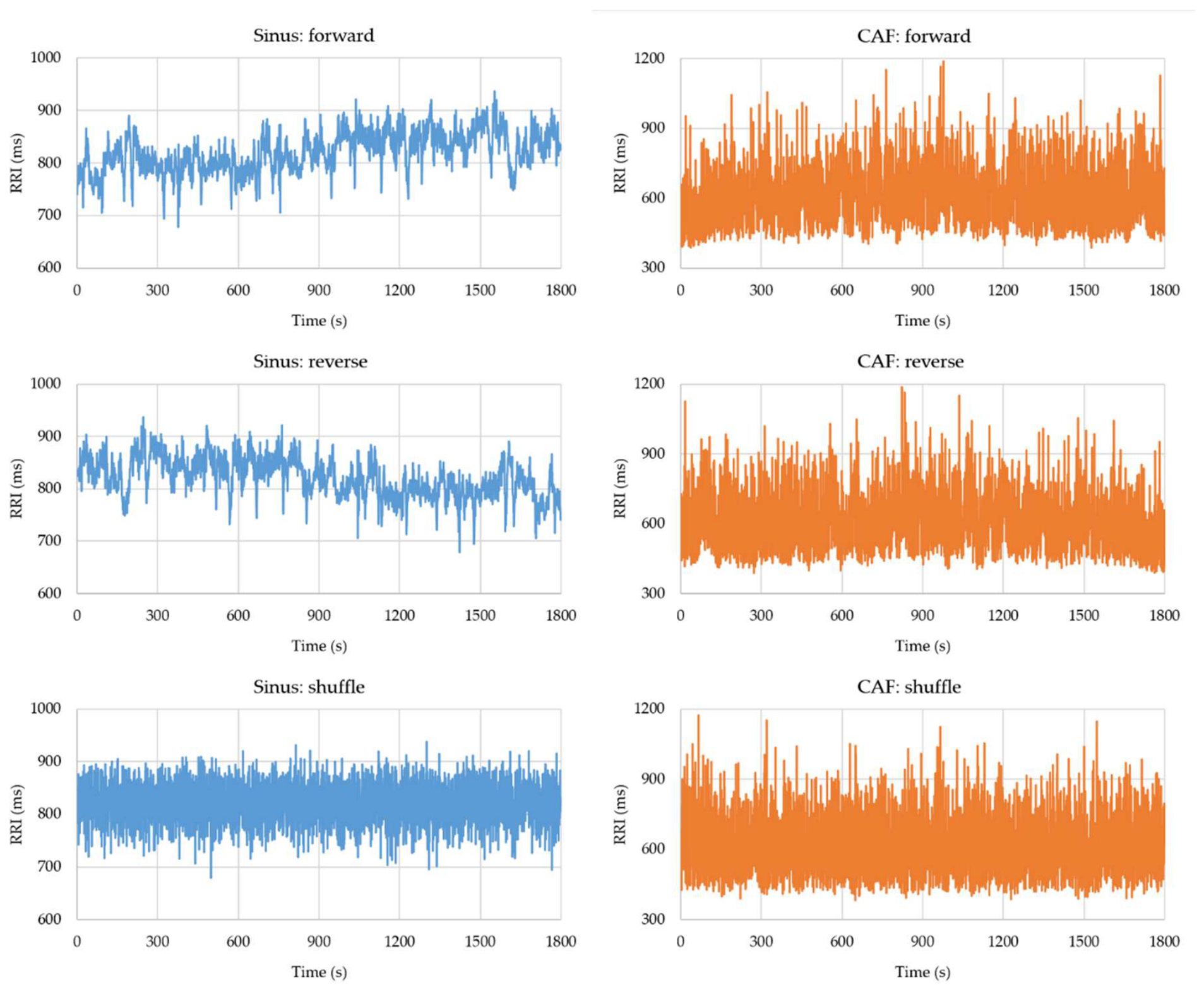
Figure 3.
Class-wise permutation importance of the top three HRV indices for the 7-HRV representation in sinus rhythm (upper panels) and CAF (lower panels). From left to right, the panels show Forward, Reverse, and Shuffle classifications.
Figure 3.
Class-wise permutation importance of the top three HRV indices for the 7-HRV representation in sinus rhythm (upper panels) and CAF (lower panels). From left to right, the panels show Forward, Reverse, and Shuffle classifications.
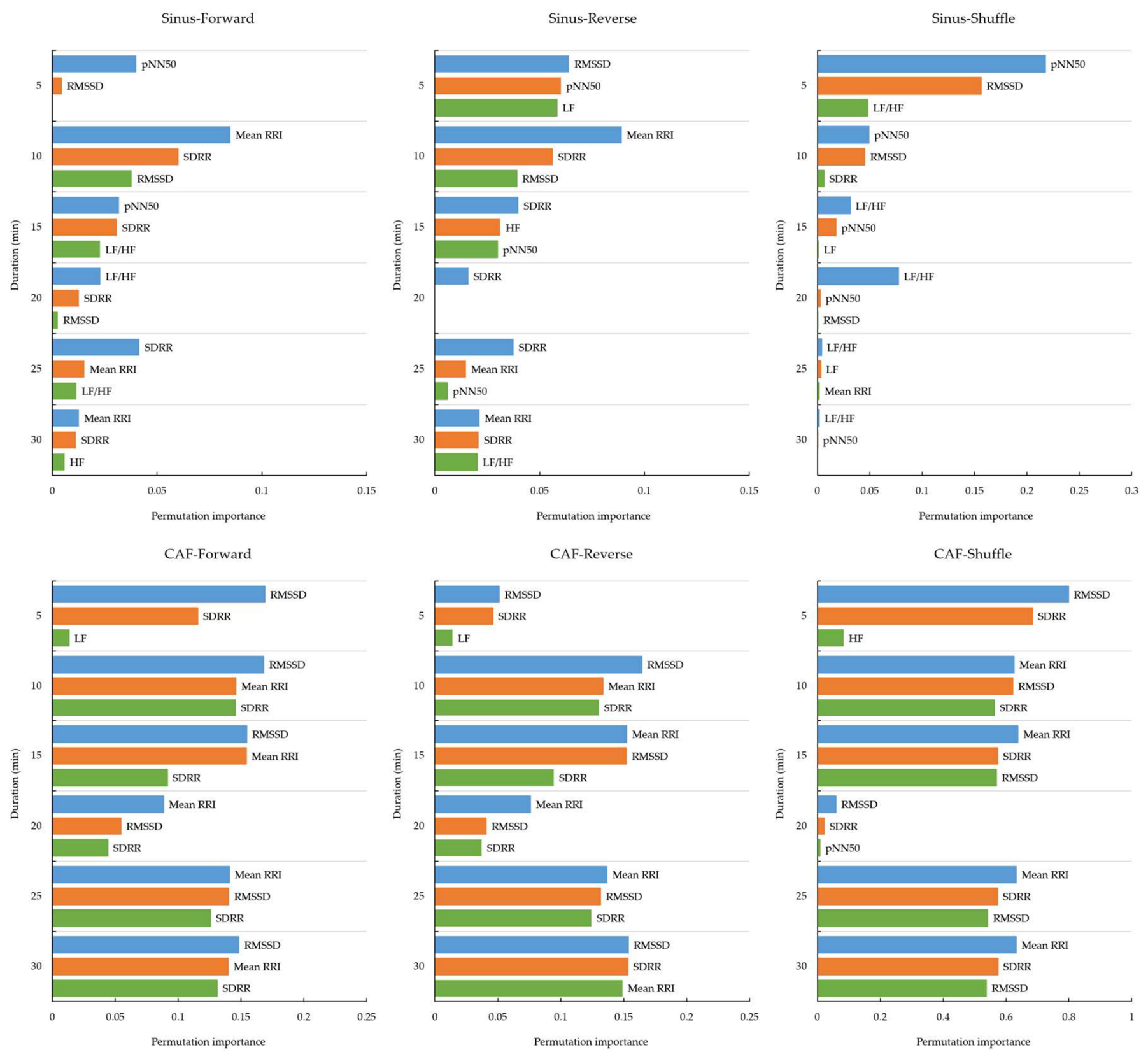
Figure 4.
Class-wise permutation importance of the top three features for the 7-HRV + temporal representation in. sinus rhythm (upper panels) and CAF (lower panels). From left to right, the panels show Forward, Reverse, and Shuffle classifications.
Figure 4.
Class-wise permutation importance of the top three features for the 7-HRV + temporal representation in. sinus rhythm (upper panels) and CAF (lower panels). From left to right, the panels show Forward, Reverse, and Shuffle classifications.
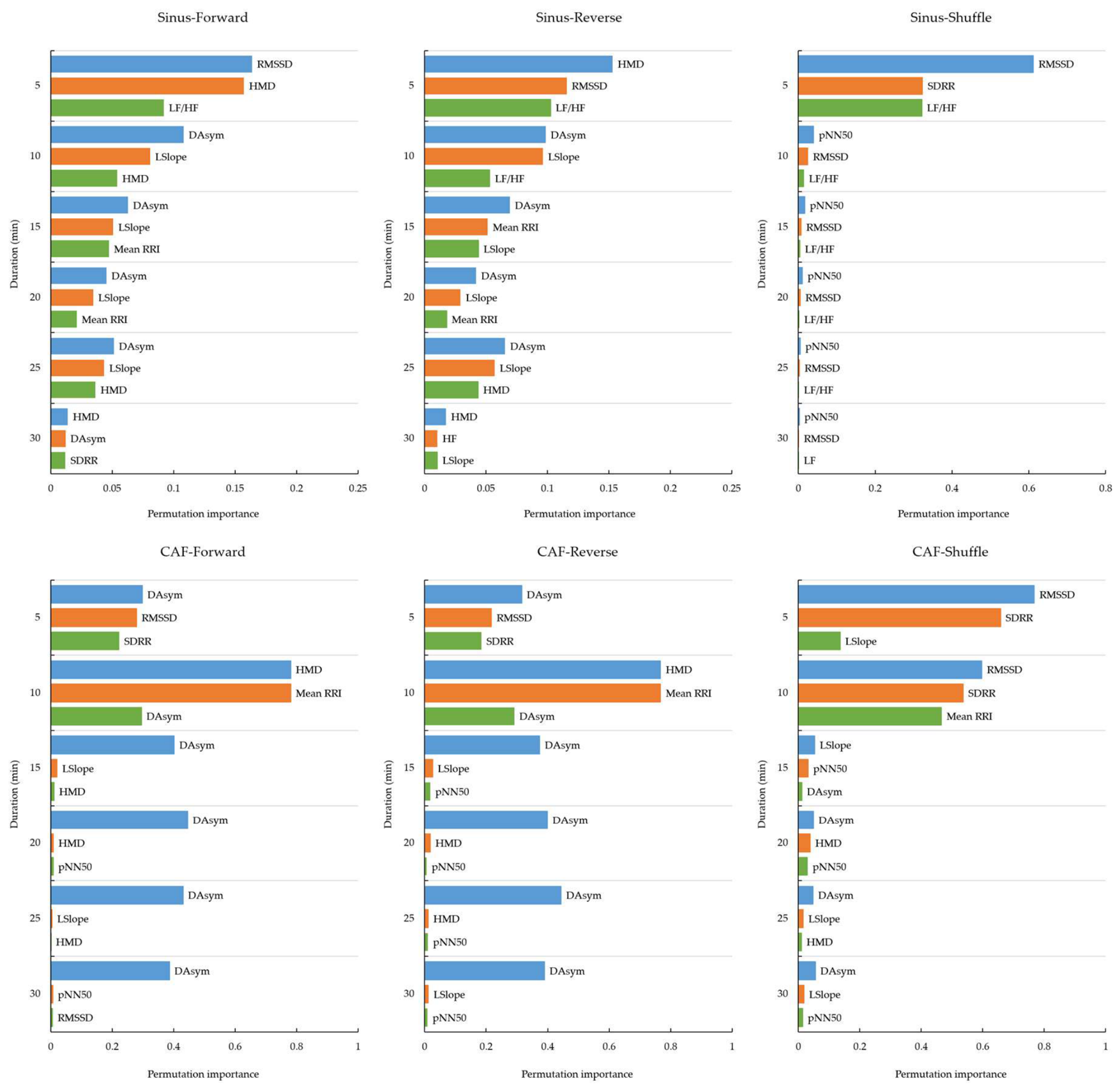
Figure 5.
Distribution of the mean magnitudes of positive and negative successive RRI changes in the original CAF sequences. Boxes indicate the interquartile range, center lines indicate the median, and whiskers extend to 1.5 times the interquartile range. Outliers are not displayed for clarity. The absolute magnitude of negative RRI changes was significantly greater than that of positive RRI changes (Wilcoxon signed-rank test, p<0.001).
Figure 5.
Distribution of the mean magnitudes of positive and negative successive RRI changes in the original CAF sequences. Boxes indicate the interquartile range, center lines indicate the median, and whiskers extend to 1.5 times the interquartile range. Outliers are not displayed for clarity. The absolute magnitude of negative RRI changes was significantly greater than that of positive RRI changes (Wilcoxon signed-rank test, p<0.001).
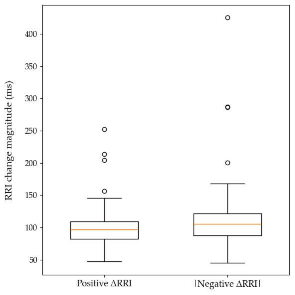
Figure 6.
Macro-F1 across input representations and observation durations in sinus rhythm and CAF. Bars indicate mean ± SD across 10 subject-wise splits. The dotted line indicates the three-class chance level (0.333). ■: Raw RRI, ■: 7-HRV, ■: 7-HRV+temporal.
Figure 6.
Macro-F1 across input representations and observation durations in sinus rhythm and CAF. Bars indicate mean ± SD across 10 subject-wise splits. The dotted line indicates the three-class chance level (0.333). ■: Raw RRI, ■: 7-HRV, ■: 7-HRV+temporal.
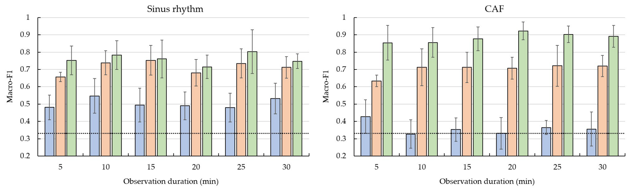

Table 1.
Characteristics of the datasets included in the analysis. For each record, Mean RRI and SDRR were calculated from the analyzed 30-min Forward RRI sequence, and the resulting record-level values are presented as mean ± SD for each dataset. For the atrial fibrillation datasets, only records containing CAF for at least 30 min were included.
Table 1.
Characteristics of the datasets included in the analysis. For each record, Mean RRI and SDRR were calculated from the analyzed 30-min Forward RRI sequence, and the resulting record-level values are presented as mean ± SD for each dataset. For the atrial fibrillation datasets, only records containing CAF for at least 30 min were included.
| Dataset | Rhythm | Included n | Age, years | Mean RRI, ms | SDRR, ms |
| Fantasia Database | Sinus | 40 | Young: 26 ± 4 Elderly: 74± 4 |
1002 ± 159 | 59 ± 27 |
| Normal Sinus Rhythm RRI Database |
Sinus | 54 | 61 ± 12 | 759 ± 105 | 74 ± 20 |
| RRI time series from healthy subjects | Sinus | 9 | 42 ± 10 | 739 ± 109 | 66 ± 28 |
| MIT-BIH AF Database | AF | 14 | Not available | 684 ± 107 | 137 ± 36 |
| Long-Term AF Database | AF | 58 | Not available | 764 ± 276 | 198 ± 177 |
| SHDB-derived cohort | AF | 50 | 70 ± 11 | 667 ± 198 | 136 ± 42 |
Table 2.
Machine-learning classifiers and fixed settings.
| Classifier | Main settings | Scaling |
| XGBoost | 300 estimators; maximum depth = 3; learning rate = 0.05; multiclass soft- probability objective |
None |
| LGR | L2 regularization; (C=1.0); L-BFGS solver; maximum 5000 iterations |
StandardScaler |
| QDA | Default settings | None |
| NB | Default settings | None |
| KNN | (k=5); Euclidean distance | StandardScaler |
| LDA | Default settings | None |
Table 3.
Classification performance using raw RRI sequences in sinus rhythm and CAF.
| Rhythm | Duration | Classifier | Accuracy | Macro-F1 | Macro-AUC |
| Sinus | 5 min | XGB | 0.485 ± 0.070 | 0.481 ± 0.071 | 0.661 ± 0.062 |
| 10 min | NB | 0.548 ± 0.100 | 0.547 ± 0.100 | 0.689 ± 0.099 | |
| 15 min | NB | 0.500 ± 0.097 | 0.494 ± 0.098 | 0.656 ± 0.076 | |
| 20 min | NB | 0.491 ± 0.083 | 0.490 ± 0.081 | 0.669 ± 0.077 | |
| 25 min | NB | 0.479 ± 0.083 | 0.480 ± 0.083 | 0.708 ± 0.077 | |
| 30 min | NB | 0.530 ± 0.085 | 0.532 ± 0.088 | 0.718 ± 0.058 | |
| CAF | 5 min | NB | 0.438 ± 0.099 | 0.428 ± 0.097 | 0.602 ± 0.088 |
| 10 min | LGR | 0.338 ± 0.089 | 0.327 ± 0.082 | 0.488 ± 0.094 | |
| 15 min | LGR | 0.354 ± 0.069 | 0.353 ± 0.068 | 0.513 ± 0.088 | |
| 20 min | QDA | 0.331 ± 0.089 | 0.331 ± 0.091 | 0.498 ± 0.067 | |
| 25 min | LGR | 0.369 ± 0.039 | 0.365 ± 0.040 | 0.543 ± 0.060 | |
| 30 min | QDA | 0.356 ± 0.098 | 0.356 ± 0.098 | 0.517 ± 0.073 |
Table 4.
Confusion matrices and permutation-test results for the raw RRI representation.
| Rhythm | Duration | Permutation p | True class | Pred. Forward | Pred. Reverse | Pred. Shuffle |
| Sinus | 5 min | <0.001 | Forward | 0.518 | 0.218 | 0.264 |
| Reverse | 0.200 | 0.582 | 0.218 | |||
| Shuffle | 0.282 | 0.364 | 0.355 | |||
| 10 min | <0.001 | Forward | 0.518 | 0.264 | 0.218 | |
| Reverse | 0.273 | 0.509 | 0.218 | |||
| Shuffle | 0.155 | 0.227 | 0.618 | |||
| 15 min | <0.001 | Forward | 0.482 | 0.218 | 0.300 | |
| Reverse | 0.236 | 0.491 | 0.273 | |||
| Shuffle | 0.200 | 0.273 | 0.527 | |||
| 20 min | <0.001 | Forward | 0.509 | 0.327 | 0.164 | |
| Reverse | 0.336 | 0.518 | 0.145 | |||
| Shuffle | 0.327 | 0.227 | 0.445 | |||
| 25 min | <0.001 | Forward | 0.518 | 0.400 | 0.082 | |
| Reverse | 0.409 | 0.518 | 0.073 | |||
| Shuffle | 0.282 | 0.318 | 0.400 | |||
| 30 min | <0.001 | Forward | 0.555 | 0.336 | 0.109 | |
| Reverse | 0.327 | 0.555 | 0.118 | |||
| Shuffle | 0.309 | 0.209 | 0.482 | |||
| CAF | 5 min | <0.001 | Forward | 0.546 | 0.331 | 0.123 |
| Reverse | 0.369 | 0.500 | 0.131 | |||
| Shuffle | 0.315 | 0.415 | 0.269 | |||
| 10 min | 0.447 | Forward | 0.446 | 0.315 | 0.238 | |
| Reverse | 0.323 | 0.338 | 0.338 | |||
| Shuffle | 0.392 | 0.377 | 0.231 | |||
| 15 min | 0.265 | Forward | 0.346 | 0.338 | 0.315 | |
| Reverse | 0.385 | 0.338 | 0.277 | |||
| Shuffle | 0.338 | 0.285 | 0.377 | |||
| 20 min | 0.548 | Forward | 0.323 | 0.377 | 0.300 | |
| Reverse | 0.331 | 0.338 | 0.331 | |||
| Shuffle | 0.300 | 0.369 | 0.331 | |||
| 25 min | 0.135 | Forward | 0.331 | 0.385 | 0.285 | |
| Reverse | 0.423 | 0.346 | 0.231 | |||
| Shuffle | 0.323 | 0.246 | 0.431 | |||
| 30 min | 0.188 | Forward | 0.423 | 0.292 | 0.285 | |
| Reverse | 0.323 | 0.308 | 0.369 | |||
| Shuffle | 0.308 | 0.354 | 0.338 |
Table 5.
Classification performance using the 7-HRV representation in sinus rhythm and CAF.
| Rhythm | Duration | Best classifier | Accuracy | Macro-F1 | Macro-AUC |
| Sinus | 5 min | KNN | 0.661 ± 0.028 | 0.657 ± 0.027 | 0.830 ± 0.014 |
| 10 min | LGR | 0.739 ± 0.070 | 0.739 ± 0.070 | 0.888 ± 0.041 | |
| 15 min | XGB | 0.755 ± 0.086 | 0.753 ± 0.086 | 0.891 ± 0.055 | |
| 20 min | XGB | 0.685 ± 0.076 | 0.681 ± 0.077 | 0.854 ± 0.038 | |
| 25 min | XGB | 0.736 ± 0.083 | 0.735 ± 0.084 | 0.887 ± 0.050 | |
| 30 min | XGB | 0.715 ± 0.063 | 0.712 ± 0.063 | 0.866 ± 0.037 | |
| CAF | 5 min | QDA | 0.656 ± 0.013 | 0.634 ± 0.034 | 0.833 ± 0.002 |
| 10 min | QDA | 0.715 ± 0.104 | 0.713 ± 0.106 | 0.857 ± 0.062 | |
| 15 min | QDA | 0.710 ± 0.090 | 0.712 ± 0.087 | 0.829 ± 0.057 | |
| 20 min | LGR | 0.710 ± 0.058 | 0.707 ± 0.063 | 0.860 ± 0.033 | |
| 25 min | QDA | 0.721 ± 0.117 | 0.721 ± 0.118 | 0.860 ± 0.055 | |
| 30 min | QDA | 0.718 ± 0.062 | 0.720 ± 0.061 | 0.834 ± 0.046 |
Table 6.
Confusion matrices and permutation-test results for the best 7-HRV classifiers.
| Rhythm | Duration | Permutation p | True class | Pred. Forward | Pred. Reverse | Pred. Shuffle |
| Sinus | 5 min | <0.001 | Forward | 0.473 | 0.527 | 0.000 |
| Reverse | 0.491 | 0.509 | 0.000 | |||
| Shuffle | 0.000 | 0.000 | 1.000 | |||
| 10 min | <0.001 | Forward | 0.609 | 0.391 | 0.000 | |
| Reverse | 0.391 | 0.609 | 0.000 | |||
| Shuffle | 0.000 | 0.000 | 1.000 | |||
| 15 min | <0.001 | Forward | 0.609 | 0.391 | 0.000 | |
| Reverse | 0.345 | 0.655 | 0.000 | |||
| Shuffle | 0.000 | 0.000 | 1.000 | |||
| 20 min | <0.001 | Forward | 0.518 | 0.482 | 0.000 | |
| Reverse | 0.464 | 0.536 | 0.000 | |||
| Shuffle | 0.000 | 0.000 | 1.000 | |||
| 25 min | <0.001 | Forward | 0.627 | 0.364 | 0.009 | |
| Reverse | 0.391 | 0.600 | 0.009 | |||
| Shuffle | 0.009 | 0.009 | 0.982 | |||
| 30 min | <0.001 | Forward | 0.545 | 0.455 | 0.000 | |
| Reverse | 0.400 | 0.600 | 0.000 | |||
| Shuffle | 0.000 | 0.000 | 1.000 | |||
| CAF | 5 min | <0.001 | Forward | 0.546 | 0.438 | 0.015 |
| Reverse | 0.546 | 0.438 | 0.015 | |||
| Shuffle | 0.015 | 0.000 | 0.985 | |||
| 10 min | <0.001 | Forward | 0.577 | 0.400 | 0.023 | |
| Reverse | 0.392 | 0.577 | 0.031 | |||
| Shuffle | 0.000 | 0.008 | 0.992 | |||
| 15 min | <0.001 | Forward | 0.577 | 0.423 | 0.000 | |
| Reverse | 0.423 | 0.577 | 0.000 | |||
| Shuffle | 0.015 | 0.008 | 0.977 | |||
| 20 min | <0.001 | Forward | 0.600 | 0.354 | 0.046 | |
| Reverse | 0.369 | 0.577 | 0.054 | |||
| Shuffle | 0.015 | 0.031 | 0.954 | |||
| 25 min | <0.001 | Forward | 0.592 | 0.408 | 0.000 | |
| Reverse | 0.408 | 0.592 | 0.000 | |||
| Shuffle | 0.000 | 0.023 | 0.977 | |||
| 30 min | <0.001 | Forward | 0.577 | 0.423 | 0.000 | |
| Reverse | 0.385 | 0.615 | 0.000 | |||
| Shuffle | 0.000 | 0.038 | 0.962 |
Table 7.
Classification performance using the 7-HRV + temporal representation in sinus rhythm and CAF.
Table 7.
Classification performance using the 7-HRV + temporal representation in sinus rhythm and CAF.
| Rhythm | Duration | Best classifier | Accuracy | Macro-F1 | Macro AUC |
| Sinus | 5 min | QDA | 0.752 ± 0.083 | 0.752 ± 0.083 | 0.877 ± 0.046 |
| 10 min | KNN | 0.785 ± 0.083 | 0.784 ± 0.083 | 0.901 ± 0.052 | |
| 15 min | KNN | 0.761 ± 0.109 | 0.761 ± 0.109 | 0.880 ± 0.070 | |
| 20 min | KNN | 0.715 ± 0.067 | 0.715 ± 0.068 | 0.875 ± 0.048 | |
| 25 min | KNN | 0.803 ± 0.126 | 0.803 ± 0.126 | 0.900 ± 0.062 | |
| 30 min | KNN | 0.748 ± 0.043 | 0.748 ± 0.042 | 0.894 ± 0.023 | |
| CAF | 5 min | QDA | 0.854 ± 0.101 | 0.854 ± 0.100 | 0.952 ± 0.044 |
| 10 min | QDA | 0.859 ± 0.083 | 0.856 ± 0.086 | 0.945 ± 0.046 | |
| 15 min | XGB | 0.877 ± 0.069 | 0.877 ± 0.069 | 0.969 ± 0.028 | |
| 20 min | XGB | 0.923 ± 0.051 | 0.923 ± 0.052 | 0.976 ± 0.021 | |
| 25 min | XGB | 0.903 ± 0.048 | 0.903 ± 0.048 | 0.975 ± 0.024 | |
| 30 min | XGB | 0.892 ± 0.063 | 0.892 ± 0.063 | 0.971 ± 0.024 |
Table 8.
Confusion matrices and permutation-test results for the 7-HRV + temporal representation.
| Rhythm | Duration | Permutation p | True class | Pred. Forward | Pred. Reverse | Pred. Shuffle |
| Sinus | 5 min | <0.001 | Forward | 0.627 | 0.373 | 0.000 |
| Reverse | 0.373 | 0.627 | 0.000 | |||
| Shuffle | 0.000 | 0.000 | 1.000 | |||
| 10 min | <0.001 | Forward | 0.691 | 0.300 | 0.009 | |
| Reverse | 0.327 | 0.664 | 0.009 | |||
| Shuffle | 0.000 | 0.000 | 1.000 | |||
| 15 min | <0.001 | Forward | 0.645 | 0.355 | 0.000 | |
| Reverse | 0.355 | 0.645 | 0.000 | |||
| Shuffle | 0.000 | 0.009 | 0.991 | |||
| 20 min | <0.001 | Forward | 0.582 | 0.418 | 0.000 | |
| Reverse | 0.427 | 0.573 | 0.000 | |||
| Shuffle | 0.000 | 0.009 | 0.991 | |||
| 25 min | <0.001 | Forward | 0.709 | 0.291 | 0.000 | |
| Reverse | 0.291 | 0.709 | 0.000 | |||
| Shuffle | 0.009 | 0.000 | 0.991 | |||
| 30 min | <0.001 | Forward | 0.618 | 0.382 | 0.000 | |
| Reverse | 0.364 | 0.636 | 0.000 | |||
| Shuffle | 0.009 | 0.000 | 0.991 | |||
| CAF | 5 min | <0.001 | Forward | 0.785 | 0.192 | 0.023 |
| Reverse | 0.200 | 0.785 | 0.015 | |||
| Shuffle | 0.000 | 0.008 | 0.992 | |||
| 10 min | <0.001 | Forward | 0.823 | 0.154 | 0.023 | |
| Reverse | 0.208 | 0.762 | 0.031 | |||
| Shuffle | 0.008 | 0.000 | 0.992 | |||
| 15 min | <0.001 | Forward | 0.815 | 0.100 | 0.085 | |
| Reverse | 0.108 | 0.854 | 0.038 | |||
| Shuffle | 0.008 | 0.031 | 0.962 | |||
| 20 min | <0.001 | Forward | 0.908 | 0.092 | 0.000 | |
| Reverse | 0.092 | 0.877 | 0.031 | |||
| Shuffle | 0.015 | 0.000 | 0.985 | |||
| 25 min | <0.001 | Forward | 0.900 | 0.054 | 0.046 | |
| Reverse | 0.077 | 0.892 | 0.031 | |||
| Shuffle | 0.062 | 0.023 | 0.915 | |||
| 30 min | <0.001 | Forward | 0.854 | 0.108 | 0.038 | |
| Reverse | 0.123 | 0.854 | 0.023 | |||
| Shuffle | 0.023 | 0.008 | 0.969 |
Disclaimer/Publisher’s Note: The statements, opinions and data contained in all publications are solely those of the individual author(s) and contributor(s) and not of MDPI and/or the editor(s). MDPI and/or the editor(s) disclaim responsibility for any injury to people or property resulting from any ideas, methods, instructions or products referred to in the content. |
© 2026 by the author. Licensee MDPI, Basel, Switzerland. This article is an open access article distributed under the terms and conditions of the Creative Commons Attribution (CC BY) license.
Copyright: This open access article is published under a Creative Commons CC BY 4.0 license, which permit the free download, distribution, and reuse, provided that the author and preprint are cited in any reuse.