

Submitted:
05 September 2026
Posted:
08 September 2026
You are already at the latest version
Abstract
Ground magnetic data were used to investigate crustal magnetic structure beneath the Ulaanbaatar region of central Mongolia. Residual total-field anomalies were analyzed using reduction to the pole, magnetic derivatives, spectral source-depth estimation, and three-dimensional susceptibility inversion. The magnetic field is characterized by short-wavelength anomalies in the south and southeast and broader magnetic domains toward the north. Spectral analysis produces characteristic source-top depths of approximately 3–5 km, centroid depths of 7–10 km, and derived basal depths of about 10–15 km; these values are interpreted as statistical source-depth parameters rather than Curie-point depths. The three-dimensional inversion reproduces the observations with an RMS residual of 2.59 nT and resolves numerous localized upper-crustal susceptibility bodies that merge into fewer, broader domains with depth. Several magnetic boundaries extend beyond mapped lithological contacts and coincide spatially with major structures. In particular, the Avdar and Sharkhai faults are preferentially associated with susceptibility gradients and magnetic-domain boundaries, consistent with reactivation of pre-existing crustal heterogeneity. These results define a three-dimensional magnetic framework for the faulted and repeatedly intruded crust beneath Ulaanbaatar.
Keywords:
magnetic susceptibility inversion
; spectral analysis
; crustal architecture
; active faults
; Ulaanbaatar region
1. Introduction
Magnetic anomalies afford essential constraints on continental crustal structure because variations in magnetic susceptibility reflect changes in lithology, magnetic-mineral abundance, intrusive history, and deformation (Telford et al. 1990,Blakely 1995,Clark 1997,Nabighian et al. 2005). Reduction to the pole (RTP) and derivative-based enhancement can sharpen anomaly patterns and emphasize source boundaries at different spatial scales (Cordell and Grauch 1985,Roest et al. 1992,Miller and Singh 1994). Three-dimensional susceptibility inversion extends this interpretation into the subsurface by recovering a volumetric model consistent with the measured field (Li and Oldenburg 1996). Spectral analysis provides a complementary statistical estimate of characteristic magnetic-source depths (Spector and Grant 1970).
Mongolia occupies a central part of the Central Asian Orogenic Belt (CAOB), where Paleozoic accretion, repeated magmatism, and later intracontinental deformation produced a strongly heterogeneous crust (Badarch et al. 2002,Windley et al. 2007). In the Ulaanbaatar region, Paleozoic sedimentary and igneous successions are juxtaposed with granitoid massifs, younger volcanic rocks, Cenozoic basin fill, and major fault systems (Kurihara et al. 2009,Sodnom et al. 2012,Ganbat et al. 2021). Regional gravity, seismic, and magnetotelluric studies have demonstrated substantial crustal and lithospheric heterogeneity in central Mongolia (Buyantogtokh et al. 2019,Guy et al. 2024), but the three-dimensional magnetic structure beneath Ulaanbaatar remains comparatively poorly constrained.
The ground magnetic field across the region contains both short- and long-wavelength anomalies, indicating contributions from sources at different depths. Short-wavelength features are expected mainly from shallow lithological contrasts, intrusive contacts, and structural boundaries, whereas broader anomalies may signify deeper basement domains and regional variations in magnetization (Blakely 1995,Clark 1997). Understanding the relationship between these magnetic domains, mapped granitoids, and active faults is essential for evaluating the extent to which present-day structures exploit pre-existing crustal heterogeneity.
This study integrates ground magnetic observations with reduction to the pole (RTP), analytic signal amplitude, total horizontal gradient, tilt derivative, spectral source-depth analysis, and three-dimensional susceptibility inversion. The objectives are to (1) delineate the principal magnetic domains and boundaries, (2) estimate the characteristic depth distribution of magnetic sources, (3) resolve their three-dimensional susceptibility structure, and (4) evaluate spatial relationships among magnetic architecture and the Avdar and Sharkhai active faults. The resulting model provides a quantitative framework for interpreting crustal segmentation and structural inheritance beneath the Ulaanbaatar region.
2. Geological Setting
The Ulaanbaatar region lies within the Khangay–Khentey sector of the Central Asian Orogenic Belt (CAOB), where Paleozoic accretionary complexes, granitoid intrusions, younger volcanic rocks, and Cenozoic sediments are juxtaposed across a complex fault network (Badarch et al. 2002,Windley et al. 2007,Erdenechimeg et al. 2018). Older consolidated rocks form most surrounding uplands, whereas Quaternary deposits occupy the Ulaanbaatar basin, the Tuul River valley, and other low-lying areas (Figure 1a) (Takeuchi et al. 2013,Batsaikhan et al. 2018,Tumurbaatar et al. 2019).
2.1. Lithological Framework
The oldest exposed units include Neoproterozoic to early Paleozoic sedimentary and metamorphic rocks composed of sandstone, siltstone, shale, carbonate rocks, schist, gneiss, marble, and locally amphibolitic assemblages (Badarch et al. 2002,Erdenechimeg et al. 2018). Paleozoic clastic, siliceous, carbonate, and volcanic rock successions are widespread in the central and northern parts of the region and include sandstone, mudstone, shale, radiolarian chert, basalt, and subordinate limestone (Kurihara et al. 2009,Takeuchi et al. 2013,Nakane et al. 2012). Components of the Gorkhi Formation have been interpreted as remnants of Paleozoic oceanic and subduction–accretion complexes (Kurihara et al. 2009). Devonian–Carboniferous granitoids intruded this heterogeneous basement, followed by additional Late Triassic–Early Jurassic granitoids and Cretaceous volcanic and volcano-sedimentary rocks (Badarch et al. 2002,Erdenechimeg et al. 2018). Those contrasting rock assemblages provide a strong basis for lateral variations in magnetic susceptibility.
2.2. Granitic Massifs and Magmatic Architecture
Granitic and granodioritic massifs are prominent around Ulaanbaatar (Sodnom et al. 2012,Erdenechimeg et al. 2018). The Bogd Uul pluton immediately south of the city consists mainly of Late Triassic–Early Jurassic biotite and hornblende–biotite granite (Sodnom et al. 2012). Surface contacts between granitoids and older country rocks commonly coincide with structural discontinuities, but their mapped outlines do not necessarily represent the geometry of the intrusive bodies at depth. The coexistence of Paleozoic and Mesozoic granitoids records multiple phases of magmatic reworking within the Khangay–Khentey region (Badarch et al. 2002,Ganbat et al. 2021,Erdenechimeg et al. 2018).
2.3. Fault Systems and Cenozoic Cover
Numerous faults cut the Paleozoic basement and younger intrusive complexes. Prominent NW–SE- and NE–SW-trending structures divide parts of the region into fault-bounded blocks, and brittle deformation includes fractured zones, fault gouge, and brecciation (Takeuchi et al. 2013,Nuramkhaan et al. 2012). Active or recently recognized fault systems surrounding Ulaanbaatar include the Ulaanbaatar, Sharkhai, Avdar, and related structures (Suzuki et al. 2020,Al-Ashkar et al. 2022). Some traces are clearly expressed at the surface, whereas others are discontinuous or masked beneath younger deposits (Al-Ashkar et al. 2022).
Cenozoic, particularly Quaternary, sediments fill the principal valleys and depressions. Unconsolidated to weakly consolidated alluvial and fluvial deposits in the Ulaanbaatar basin and Tuul River corridor locally reach substantial thicknesses and conceal bedrock contacts and fault traces (Batsaikhan et al. 2018,Tumurbaatar et al. 2019,Al-Ashkar et al. 2022). The study area therefore combines heterogeneous accretionary basement, multiphase granitoid magmatism, active faulting, and sedimentary cover, providing the geological framework for the magnetic interpretation below.
3. Data and Methods
3.1. Ground Magnetic Data and Processing
Ground magnetic observations acquired across an approximately km area surrounding Ulaanbaatar were used to characterize crustal magnetization. The measured total magnetic intensity (TMI) contains the crustal signal, temporal geomagnetic variations, and the Earth’s main field.
Temporal variations were corrected using simultaneous magnetic records from a nearby reference station. The reference variation was interpolated to the acquisition time of each field measurement and removed from the observed TMI. The main geomagnetic field was subsequently calculated for the location, elevation, and acquisition epoch of each observation using the International Geomagnetic Reference Field (IGRF) (Beggan et al. 2026). The corrected residual magnetic anomaly was defined as
where is the measured total field, represents temporal geomagnetic variation, and is the modeled main field. The resulting residual field primarily represents spatial variations in crustal magnetization.
Quality control included removal of duplicate observations, verification of coordinates and elevations, and inspection for instrumental and cultural noise. Isolated values exceeding nT were excluded where they were inconsistent with surrounding measurements. The corrected residual magnetic anomaly field is shown in Figure 1b, whereas the observation locations used in the inversion are shown in Figure 5a.
3.2. Reduction to the Pole and Magnetic-Field Enhancement
The residual magnetic field was transformed by reduction to the pole (RTP) to reduce the lateral displacement among magnetic anomalies and their causative sources (Baranov and Naudy 1964). The Fourier-domain transformation used geomagnetic parameters representative of the survey area and acquisition period, with a field intensity of approximately nT, inclination of , and declination of . The RTP field was used for comparison with mapped lithologies, granitoid massifs, and structural boundaries.
Derivative-based attributes were calculated from the RTP field to enhance lateral changes in magnetization. The total horizontal gradient (THG), analytic signal amplitude (ASA), and tilt derivative (TDR) were defined as
where T denotes the RTP anomaly. THG emphasizes strong lateral susceptibility contrasts and is useful for locating magnetic-source boundaries (Cordell and Grauch 1985). ASA combines horizontal and vertical gradients and provides complementary delineation of source edges with reduced dependence on anomaly polarity (Roest et al. 1992). TDR normalizes the vertical derivative by the horizontal gradient and improves both strong and weak magnetic boundaries (Miller and Singh 1994).
3.3. Spectral Analysis of Magnetic-Source Depths
Spectral analysis was applied to estimate the characteristic depths of magnetic-source populations. The method follows the statistical spectral framework of Spector and Grant (1970), in which magnetic anomalies generated by ensembles of sources at different depths produce characteristic slopes in the radially averaged power spectrum.
The two-dimensional Fourier transform of the magnetic anomaly grid was calculated and converted to a power spectrum,
where is the two-dimensional Fourier transform of the magnetic field. The spectrum was radially averaged according to the horizontal angular wavenumber
where and are spatial frequencies in cycles per kilometre and k is expressed in radians per kilometre.
Following the spectral source-depth formulation of Spector and Grant (1970) and Tanaka et al. (1999), characteristic top and centroid depths were estimated from linear portions of the radially averaged spectrum. The source-top depth was obtained from the higher-wavenumber interval,
whereas the centroid depth was estimated from the lower-wavenumber interval,
A derived basal source-depth parameter was then calculated as
where is the characteristic source-top depth and is the centroid depth. The same procedure was applied across overlapping spatial windows, and the accepted estimates were interpolated to construct the regional depth maps. These values are interpreted as effective source-depth parameters rather than precise geological interfaces; in this study, is not interpreted as a Curie-point depth.
The finite dimensions of the survey impose an important limitation on the lowest resolvable wavenumbers. With a survey extent of approximately km, the longest wavelengths are represented by relatively few independent spectral components and consequently provide limited resolution of very deep sources. The deepest estimates were therefore interpreted conservatively. The analysis was not used to determine Curie-point depth or the thermal base of crustal magnetization; it was used only to characterize the probable depth distribution of magnetic sources.
3.4. Three-Dimensional Magnetic Susceptibility Inversion
Three-dimensional magnetic susceptibility inversion was performed using the open-source SimPEG framework (Cockett et al. 2015). The objective was to recover a volumetric susceptibility distribution capable of reproducing the principal features of the observed magnetic field and to evaluate the subsurface geometry of the magnetic domains identified from the surface anomaly maps.
The inversion used the corrected residual TMI rather than the RTP-transformed field. This preserves the real observation geometry and avoids propagating assumptions introduced by the RTP transformation into the inverse problem. RTP and derivative products were instead used independently for structural interpretation.
Assuming predominantly induced magnetization parallel to the regional geomagnetic field, the total-field magnetic field can be expressed as (Li and Oldenburg 1996)
where is the predicted magnetic-data vector, is the magnetic sensitivity operator, and contains the susceptibility values assigned to the active model cells.
Because magnetic inversion is non-unique, the susceptibility model was recovered through regularized optimization following the formulation of Li and Oldenburg (1996). The objective function was
where contains the inverse data uncertainties, controls model elaboration, and determines the trade-off between fitting the observations and obtaining a geologically reasonable model. The regularization included model-smallness and spatial-smoothness terms in the three coordinate directions, favouring a coherent susceptibility distribution while allowing contrasts required by the observations.
The model domain extended laterally beyond the observation area and to approximately 30 km depth to minimize boundary influences. Survey elevations were incorporated directly into the forward calculation, and cells above the topographic surface were excluded from the active model. Sensitivity weighting was applied to compensate for the rapid decrease in magnetic sensitivity with source depth, as a result reducing artificial concentration of susceptibility immediately beneath the observations (Li and Oldenburg 1996).
A bounded susceptibility inversion was solved iteratively using a projected Gauss–Newton conjugate-gradient optimization scheme implemented in SimPEG (Cockett et al. 2015). Iterations progressively reduced the weighted data misfit while satisfying the imposed model regularization and susceptibility bounds. The final model is therefore one regularized susceptibility distribution consistent with the observations, not a unique reconstruction of subsurface geology.
Normalized residuals were evaluated using
where is the data uncertainty used in . Because the inversion assumes predominantly induced magnetization, localized remanent contributions cannot be excluded; the recovered values are therefore interpreted as effective susceptibility.
The recovered model was interpreted jointly with the geological map, RTP anomaly, THG, ASA, and TDR. Agreement among independent magnetic attributes was used to evaluate the lateral continuity and depth extent of the principal susceptibility domains and their spatial relationships with granitoid massifs, lithological boundaries, and regional fault systems.
3.5. Active-fault association analysis
The relationship between active faults and magnetic structure was quantified from the three-dimensional susceptibility model. The horizontal susceptibility-gradient magnitude was calculated as
where is magnetic susceptibility. For the Avdar and Sharkhai faults, median and susceptibility were calculated within 2.5 km of each fault and compared with a local background 5–20 km from the fault. The corresponding enrichment ratios were
Ratios greater than unity indicate preferential association with enhanced gradients or susceptibility. Magnetic-boundary orientations were extracted from the horizontal susceptibility-gradient field and compared with mapped fault strikes using axial angular differences weighted by the local gradient magnitude.
4. Results
4.1. RTP Magnetic Anomalies and Structural Derivatives
The reduced-to-pole (RTP) magnetic field shows pronounced spatial variability across the Ulaanbaatar region (Figure 2a). Broad negative anomalies dominate much of the northern and northeastern parts of the survey, whereas positive anomalies are more prominent in the west-central sector and occur discontinuously through the central and southern areas. The southern part of the survey contains a denser distribution of short-wavelength positive and negative anomalies, with particularly strong local variations in the southeast. In contrast, the northern sector is characterized by larger and more spatially continuous anomaly patterns.
The analytic signal amplitude exhibits a strongly localized distribution of high-gradient zones (Figure 2b). The largest amplitudes occur in the southern and southeastern parts of the survey, including several compact maxima between approximately E and E. Additional localized maxima occur along the northeastern and northwestern margins. Much of the central and northern survey area is characterized by comparatively low analytic-signal amplitudes, interrupted by isolated compact or elongated high-amplitude features.
The total horizontal gradient (THG) shows a broadly similar spatial distribution but resolves many of the enhanced zones as narrower and more sharply defined features (Figure 2c). Strong gradients are particularly prominent in the southeastern part of the survey and along the northeastern margin, with additional localized zones distributed across the western and central sectors. Several elongated gradient features display approximately NW–SE, NE–SW, and locally E–W orientations. Lower THG values occupy much of the north-central and central-eastern parts of the map.
The tilt derivative shows alternating positive and negative domains across most of the survey area (Figure 2d). Broad negative values characterize much of the northern sector, whereas the central and southern parts contain more closely spaced and elongated positive and negative bands. Sharp transitions between adjacent tilt domains are particularly evident in the central, south-central, and southeastern sectors. Compared to the RTP map, the tilt-derivative image resolves a greater number of narrow and laterally continuous features over areas of both high and subdued magnetic amplitude.
Collectively, these four products distinguish broad, relatively smooth anomalies in the north from a denser set of short-wavelength features in the central and southern sectors. The derivative maps reveal many of these features as laterally continuous boundaries with dominant NW–SE, NE–SW, and locally E–W orientations.
4.2. Depth Distribution of Magnetic Sources
Spectral analysis presents systematic spatial variations in characteristic magnetic-source depths beneath the Ulaanbaatar region. A representative spectral window is shown in Figure 3. The fitted spectral segments yield a top depth of km and a centroid depth of km, corresponding to a derived source depth of km. The coefficients of fit are for the fit and for the fit.
The spatial distribution of varies from approximately 3 to 5 km across the study area (Figure 4a). Values of about 3–4 km occur mainly in the western and southwestern sectors, whereas larger depths of approximately 4.5–5 km characterize much of the eastern and northeastern parts of the survey. The change between these ranges forms a broad NW–SE-oriented zone across the central part of the map.
Centroid depths () range from approximately 7 to 10 km (Figure 4b). Values below about 8 km occupy much of the southern and southeastern sectors, whereas depths of 9–10 km occur predominantly toward the north and northeast. Intermediate values extend across the central part of the survey, producing a broad lateral gradient between the southern and northern sectors.
The obtained source depths () range from approximately 10 to 15 km (Figure 4c). The smallest values, generally around 10–12 km, occur across the southern and southeastern parts of the study area. Larger values of approximately 13–15 km extend across the northern and northwestern sectors. A large change between these depth ranges crosses the central part of the survey.
All three estimates show a coherent regional trend from shallower values in the south and southwest to greater depths in the north and northeast. The and maps are smoother than the distribution, but each contains a broad transition across central Ulaanbaatar.
4.3. Three-Dimensional Susceptibility Model
The recovered three-dimensional susceptibility model reproduces the principal spatial variations in the observed residual total-field magnetic anomaly (Figure 5). The predicted response closely follows both the broad anomaly pattern and the principal localized highs and lows present in the observations (Figure 5a,b). Observed-minus-predicted residuals are generally small and show no prominent regional-scale spatial trend (Figure 5c).
The final model yields an RMS residual of 2.59 nT, with and a correlation coefficient of between observed and predicted data (Figure 5d). Residuals are centered close to zero, with a mean of nT, a standard deviation of 2.59 nT, and a mean absolute error of 1.79 nT (Figure 5e). Normalized residuals are similarly concentrated around zero, with an NRMS of approximately 0.49 (Figure 5f). These statistics indicate a close fit between the observed and predicted fields within the regularized inversion framework.
Horizontal slices show substantial lateral variation in susceptibility and a progressive change in spatial scale with depth (Figure 6). At 0–4 km, the model contains numerous localized high-susceptibility features distributed within a predominantly low-susceptibility background. These features are most densely developed in the southern and southeastern parts of the model, with additional localized maxima in the northwest and near the eastern margin.
Between approximately 6 and 10 km depth, the susceptibility distribution becomes smoother and the number of isolated high-susceptibility features decreases. Broader zones remain visible in the southeastern, northwestern, and central parts of the model, while extensive areas retain comparatively low susceptibility.
At 12–16 km depth, the recovered structure is dominated by a smaller number of broad susceptibility domains. The strongest values at these levels occur mainly in the northwestern and southeastern sectors, with lower-amplitude zones extending through parts of the central region.
Vertical sections illustrate the lateral and vertical variability of the recovered susceptibility distribution (Figure 7). The east–west sections show several discrete susceptibility highs separated by broad regions of lower values. Some anomalies are concentrated within the upper 5–10 km, whereas others remain visible through multiple depth intervals and extend into the middle part of the model. The spatial coverage and amplitude of these features vary markedly between individual sections.
The north–south sections display a similarly heterogeneous pattern. Localized susceptibility maxima occur at different horizontal positions and depths, with some restricted to shallow levels and others extending through broader depth intervals. The strongest responses are concentrated in selected northern, central, and southern parts of the sections rather than forming a laterally continuous layer.
Overall, the recovered model changes from numerous localized susceptibility variations in the upper crust to fewer, broader features at greater depths. Due to the decrease in magnetic sensitivity with depth and the non-uniqueness of the inverse problem, the geometry of the deepest features is less well constrained than that of the shallow and intermediate structures (Li and Oldenburg 1996).
4.4. Active-fault relationships
The Avdar and Sharkhai faults show contrasting associations with subsurface magnetic structure (Figure 8). Within 2.5 km of the Sharkhai fault, the median susceptibility-gradient magnitude is approximately 1.96 and 1.86 times the local background at 2 and 6 km depth, respectively, and approaches background values below about 10 km. Susceptibility itself is not similarly enhanced. Avdar shows a weaker but more persistent gradient ratio of approximately 1.2–1.4 and locally elevated susceptibility at intermediate depths.
Boundary orientation provides an additional distinction. Avdar shows closer agreement between fault strike and nearby magnetic boundaries, particularly at 6 km depth, where the weighted median axial misfit is approximately . Sharkhai shows poorer directional agreement despite its strong shallow gradient association.
5. Discussion
The magnetic data resolve a crust composed of laterally distinct susceptibility domains with contrasting depth extent. Interpretation emphasizes features that are supported independently by the RTP and derivative maps, spectral estimates, and three-dimensional inversion. Because susceptibility inversion is non-unique, the model is used to define robust first-order patterns rather than exact geological boundaries (Li and Oldenburg 1996,Cockett et al. 2015).
5.1. Structural controls on magnetic architecture
The RTP and derivative maps show that major magnetic boundaries commonly cut across or go beyond mapped geological contacts (Figure 2). This relationship is also visible in the source-depth maps and susceptibility slices (Figure 4 and Figure 6). At shallow levels, strong contrasts occur near several mapped faults and granitoid margins; with increasing depth, these contrasts merge into expanded magnetic domains. The observations therefore do not support simple downward continuation of surface geological boundaries.
Faults can generate magnetic contrasts by juxtaposing rocks of different susceptibility or by modifying magnetic minerals through deformation and alteration. Accordingly, some mapped faults coincide with pronounced magnetic gradients, whereas others have little magnetic expression. Boundaries without mapped surface counterparts may represent concealed structures, intrusive contacts, or basement-domain margins. The granitoid massifs are similarly heterogeneous: individual plutons contain both high- and low-susceptibility zones, consistent with multiple phases and compositions of granitoid magmatism in central Mongolia (Ganbat et al. 2021,Jahn et al. 2004). This complexity is compatible with a CAOB crust assembled by accretion and subsequently modified by repeated magmatism and deformation (Badarch et al. 2002,Jahn et al. 2004).
5.2. Source-depth framework and three-dimensional structure
Spectral analysis places the characteristic top of the magnetic-source ensemble mainly at 3–5 km and its centroid at approximately 7–10 km, with derived basal values of about 10–15 km (Figure 3 and Figure 4). These are statistical source-depth parameters rather than discrete interfaces (Spector and Grant 1970). Their regional pattern is consistent with the inversion, which contains numerous localized susceptibility contrasts in the upper 0–4 km and fewer, broader domains between approximately 6 and 16 km (Figure 6 and Figure 7).
The two analyses provide complementary constraints. Spectral slopes characterize the average depth distribution of source populations, whereas inversion recovers a regularized three-dimensional susceptibility model. The obtained values are therefore not interpreted as Curie-point depths. Given the approximately km survey extent, the longest wavelengths are insufficiently resolved for a robust regional thermal-depth estimate. Variations in may instead reflect the combined effects of lithology, magnetic-mineral abundance, intrusive geometry, alteration, and structure.
5.3. Integrated Crustal Architecture
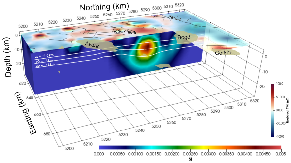
Figure 9 combines the residual magnetic field, mapped structures, spectral depth estimates, and susceptibility model. A representative contrast occurs between a relatively shallow magnetic anomaly adjacent to the Avdar fault and the larger susceptibility domain southwest of the Bogd granitoid complex. The latter persists through much of the characteristic – interval and reaches its strongest susceptibility at middle-crustal depths, indicating a subsurface magnetic body more extensive than the mapped surface expression of the Bogd granitoid.
The deeper domain could represent subsurface intrusive material, magnetically distinct basement, or a composite volume produced by repeated magmatic and tectonic modification. Magnetic data alone cannot distinguish uniquely among these alternatives. Nevertheless, the geometry demonstrates that several crustal domains continue beneath mapped contacts and younger cover. The regional magnetic architecture is therefore best interpreted as the cumulative product of Paleozoic accretion, repeated granitoid emplacement, and later deformation (Badarch et al. 2002,Ganbat et al. 2021,Jahn et al. 2004).
5.4. Implications for Active Deformation and Structural Inheritance
The contrasting relationships observed for Avdar and Sharkhai suggest that active deformation interacts with inherited magnetic framework in different ways. Sharkhai is most strongly associated with a shallow magnetic-domain boundary, whereas Avdar shows a weaker but more persistent correspondence with a magnetically distinct crustal margin (Figure 8). Paleoseismic observations demonstrate repeated late-Quaternary activity along Sharkhai (Al-Ashkar et al. 2022), and magnetic contrasts near active faults may reflect juxtaposition of different rock units or modification of magnetic minerals by deformation, fluids, and alteration (Yang et al. 2020,Villani et al. 2015).
These patterns are consistent with structural inheritance, in which later deformation preferentially exploits pre-existing faults, shear zones, or lithological boundaries established during earlier crustal assembly (Holdsworth et al. 1997). The magnetic data do not image active fault planes directly, but they show that both fault systems occupy crustal zones with pronounced lateral susceptibility changes. This provides a plausible link between inherited crustal heterogeneity and present-day deformation around Ulaanbaatar.
6. Conclusions
Ground magnetic observations, spectral analysis, and three-dimensional susceptibility inversion define a coherent crustal magnetic framework beneath the Ulaanbaatar region. The principal findings are: (1) the magnetic field is laterally segmented, with dense short-wavelength structure in the south and southeast and broader domains toward the north; (2) characteristic magnetic-source tops occur mainly at 3–5 km and centroids at 7–10 km, with estimated basal parameters of about 10–15 km; and (3) the susceptibility model changes from numerous localized upper-crustal bodies to fewer, broader domains at middle-crustal depths.
Several subsurface magnetic boundaries do not coincide directly with mapped surface contacts, indicating concealed or deeper crustal structure. The Avdar and Sharkhai faults are preferentially associated with susceptibility gradients, but in different ways: Sharkhai shows the strongest shallow gradient association, whereas Avdar shows a weaker, more persistent relationship and better strike agreement with nearby magnetic boundaries. These results are consistent with active deformation exploiting inherited crustal heterogeneity, although the magnetic boundaries should not be interpreted as direct images of fault planes.
The magnetic model provides a structural basis for future integrated geophysical interpretation. Gravity data can help distinguish density contrasts among granitoid and basement domains, magnetotelluric data can test for conductive fault zones and altered crust, and seismic constraints can refine crustal interfaces and active structures. Joint or integrated interpretation of susceptibility, density, resistivity, and seismic properties should reduce the ambiguity inherent in magnetic inversion and provide a more complete model of the tectono-magmatic architecture beneath Ulaanbaatar.
Author Contributions
T.S.Sh.: conceptualization, investigation, data curation, field data collection, formal analysis, visualization, and writing—original draft preparation. B.E.: methodology, three-dimensional magnetic modelling and inversion, resources, supervision, and writing—review and editing. O.Ch.: supervision, resources, project administration, and writing—review and editing. B.G.: data curation and resources. All authors have read and agreed to the published version of the manuscript.
Funding
This research received no external grant funding. The geophysical fieldwork and related research activities were supported through the institutional resources of the Institute of Astronomy and Geophysics, Mongolian Academy of Sciences, and were conducted within the framework of scientific cooperation between the Institute of Astronomy and Geophysics and the China Earthquake Administration.
Data Availability Statement
The magnetic data and derived products supporting the findings of this study are available from the corresponding author upon reasonable request.
Acknowledgments
The authors gratefully acknowledge Tsagaansukh Khalzan and Nasan-Ochir Tumen for their assistance with magnetic field data acquisition and field operations. The authors also acknowledge the Institute of Astronomy and Geophysics, Mongolian Academy of Sciences, for institutional and technical support during the survey and subsequent data analysis.
Conflicts of Interest
The authors declare no conflicts of interest. The funder had no role in the design of the study; in the collection, analysis, or interpretation of the data; in the writing of the manuscript; or in the decision to publish the results.
References
- Telford, W.M., L.P. Geldart, and R.E. Sheriff. 1990. Applied Geophysics, 2 ed. Cambridge: Cambridge University Press. [Google Scholar]
- Blakely, R.J. 1995. Potential Theory in Gravity and Magnetic Applications. Cambridge: Cambridge University Press. [Google Scholar] [CrossRef]
- Clark, D.A. 1997. Magnetic Petrophysics and Magnetic Petrology: Aids to Geological Interpretation of Magnetic Surveys. AGSO Journal of Australian Geology & Geophysics 17: 83–103. [Google Scholar]
- Nabighian, M.N., V.J.S. Grauch, R.O. Hansen, T.R. LaFehr, Y. Li, J.W. Peirce, J.D. Phillips, and M.E. Ruder. 2005. The Historical Development of the Magnetic Method in Exploration. Geophysics 70: 33ND–61ND. [Google Scholar] [CrossRef]
- Cordell, L., and V.J.S. Grauch. 1985. Mapping Basement Magnetization Zones from Aeromagnetic Data in the San Juan Basin, New Mexico. In The Utility of Regional Gravity and Magnetic Anomaly Maps. Edited by W.J. Hinze. Society of Exploration Geophysicists: pp. 181–197. [Google Scholar] [CrossRef]
- Roest, W.R., J. Verhoef, and M. Pilkington. 1992. Magnetic Interpretation Using the 3-D Analytic Signal. Geophysics 57: 116–125. [Google Scholar] [CrossRef]
- Miller, H.G., and V. Singh. 1994. Potential Field Tilt—A New Concept for Location of Potential Field Sources. Journal of Applied Geophysics 32: 213–217. [Google Scholar] [CrossRef]
- Li, Y., and D.W. Oldenburg. 1996. 3-D Inversion of Magnetic Data. Geophysics 61: 394–408. [Google Scholar] [CrossRef]
- Spector, A., and F.S. Grant. 1970. Statistical Models for Interpreting Aeromagnetic Data. Geophysics 35: 293–302. [Google Scholar] [CrossRef]
- Badarch, G., W.D. Cunningham, and B.F. Windley. 2002. A New Terrane Subdivision for Mongolia: Implications for the Phanerozoic Crustal Growth of Central Asia. Journal of Asian Earth Sciences 21: 87–110. [Google Scholar] [CrossRef]
- Windley, B.F., D. Alexeiev, W. Xiao, A. Kröner, and G. Badarch. 2007. Tectonic Models for Accretion of the Central Asian Orogenic Belt. Journal of the Geological Society 164: 31–47. [Google Scholar] [CrossRef]
- Kurihara, T., K. Tsukada, S. Otoh, K. Kashiwagi, C. Minjin, B. Dorjsuren, B. Bujinlkham, G. Sersmaa, N. Manchuk, M. Niwa, and et al. 2009. Upper Silurian and Devonian Pelagic Deep-Water Radiolarian Chert from the Khangai–Khentei Belt of Central Mongolia: Evidence for Middle Paleozoic Subduction–Accretion Activity in the Central Asian Orogenic Belt. Journal of Asian Earth Sciences 34: 209–225. [Google Scholar] [CrossRef]
- Sodnom, K., G. Ochir, C. Danzan, B.U. Dash, and M. Baatar. 2012. Origin of the Early Mesozoic Bogd Uul Granite Pluton, Ulaanbaatar Area, Mongolia. Bulletin of the Nagoya University Museum 28: 45–59. [Google Scholar] [CrossRef]
- Ganbat, A., T. Tsujimori, L. Miao, I. Safonova, D. Pastor-Galán, C. Anaad, M. Baatar, S. Aoki, K. Aoki, and I. Savinskiy. 2021. Late Paleozoic–Early Mesozoic Granitoids in the Khangay–Khentey Basin, Central Mongolia: Implication for the Tectonic Evolution of the Mongol–Okhotsk Ocean Margin. Lithos 404-405: 106455. [Google Scholar] [CrossRef]
- Buyantogtokh, B., E.K. Turutanov, and V.S. Kanaikin. 2019. Crustal Structure of the Ulaanbaatar Region, Mongolia According to Gravimetric Data. Geodynamics & Tectonophysics 10: 585–602. [Google Scholar] [CrossRef]
- Guy, A., C. Tiberi, and S. Mijiddorj. 2024. Crustal Structures From Receiver Functions and Gravity Modeling in Central Mongolia. Journal of Geophysical Research: Solid Earth 129: e2023JB027614. [Google Scholar] [CrossRef]
- Erdenechimeg, D., B. Enkhbayar, G. Boldbaatar, B. Damdinjav, and T. Taivanbaatar. Geological Map of Mongolia, 2018. Scale 1:500,000, Geo Information Data–2013 Project, Report No. 8480. Ulaanbaatar, Mongolia: Geological Investigation Center.
- Takeuchi, M., K. Tsukada, T. Suzuki, Y. Nakane, S. Gonchigdorj, M. Nuramkhaan, T. Kondo, N. Matsuzawa, B. Nuramkhaan, K. Sodnom, and et al. 2013. Stratigraphy and Geological Structure of the Paleozoic System around Ulaanbaatar, Mongolia. Bulletin of the Nagoya University Museum 28: 1–18. [Google Scholar]
- Batsaikhan, N., J.M. Lee, B. Nemer, and N.C. Woo. 2018. Water Resources Sustainability of Ulaanbaatar City, Mongolia. Water 10: 750. [Google Scholar] [CrossRef]
- Tumurbaatar, Z., H. Miura, and T. Tsamba. 2019. Site Effect Assessment in Ulaanbaatar, Mongolia through Inversion Analysis of Microtremor H/V Spectral Ratios. Geosciences 9: 228. [Google Scholar] [CrossRef]
- Nakane, Y., T. Kurihara, B. Nuramkhaan, M. Nuramkhaan, M. Takeuchi, K. Tsukada, S. Gonchigdorj, and K. Sodnom. 2012. Geological Division of the Rocks at Southeast of Ulaanbaatar (Gachuurt–Nalaikh), Central Mongolia. Bulletin of the Nagoya University Museum 28: 19–26. [Google Scholar]
- Nuramkhaan, B., Y. Nakane, S. Yamasaki, J. Otgonbaatar, M. Nuramkhaan, M. Takeuchi, K. Tsukada, Y. Katsurada, S. Gonchigdorj, and K. Sodnom. 2012. Description of a NW-Trending Brittle Shear Zone, Ulaanbaatar, Mongolia. Bulletin of the Nagoya University Museum 28: 39–43. [Google Scholar]
- Suzuki, Y., T. Nakata, M. Watanabe, S. Battulga, D. Enkhtaivan, S. Demberel, C. Odonbaatar, A. Bayasgalan, and T. Badral. 2020. Discovery of Ulaanbaatar Fault: A New Earthquake Threat to the Capital of Mongolia. Seismological Research Letters 92: 437–447. [Google Scholar] [CrossRef]
- Al-Ashkar, A., A. Schlupp, M. Ferry, and U. Munkhuu. 2022. Tectonic Geomorphology and Paleoseismology of the Sharkhai Fault: A New Source of Seismic Hazard for Ulaanbaatar (Mongolia). Solid Earth 13: 761–777. [Google Scholar] [CrossRef]
- Beggan, C.D., C. Kloss, P. Amblard, T. Amezza, H. Amit, J. Aubert, J. Baerenzung, and et al. 2026. International Geomagnetic Reference Field: The Fourteenth Generation. Earth, Planets and Space 78: 127. [Google Scholar] [CrossRef]
- Baranov, V., and H. Naudy. 1964. Numerical Calculation of the Formula of Reduction to the Magnetic Pole. Geophysics 29: 67–79. [Google Scholar] [CrossRef]
- Tanaka, A., Y. Okubo, and O. Matsubayashi. 1999. Curie Point Depth Based on Spectrum Analysis of the Magnetic Anomaly Data in East and Southeast Asia. Tectonophysics 306: 461–470. [Google Scholar] [CrossRef]
- Cockett, R., S. Kang, L.J. Heagy, A. Pidlisecky, and D.W. Oldenburg. 2015. SimPEG: An Open Source Framework for Simulation and Gradient Based Parameter Estimation in Geophysical Applications. Computers & Geosciences 85: 142–154. [Google Scholar] [CrossRef]
- Jahn, B.M., R. Capdevila, D. Liu, A. Vernon, and G. Badarch. 2004. Sources of Phanerozoic Granitoids in the Transect Bayanhongor–Ulaan Baatar, Mongolia: Geochemical and Nd Isotopic Evidence, and Implications for Phanerozoic Crustal Growth. Journal of Asian Earth Sciences 23: 629–653. [Google Scholar] [CrossRef]
- Yang, T., Y.M. Chou, E.C. Ferré, M.J. Dekkers, J. Chen, E.C. Yeh, W. Tanikawa, and et al. 2020. Faulting Processes Unveiled by Magnetic Properties of Fault Rocks. Reviews of Geophysics 58: e2019RG000690. [Google Scholar] [CrossRef]
- Villani, F., and et al. 2015. Imaging the Structural Style of an Active Normal Fault Through Multidisciplinary Geophysical Investigation: A Case Study from the Mw 6.1, 2009 L’Aquila Earthquake Region (Central Italy). Geophysical Journal International 200: 1676–1691. [Google Scholar] [CrossRef]
- Holdsworth, R.E., C.A. Butler, and A.M. Roberts. 1997. The Recognition of Reactivation During Continental Deformation. Journal of the Geological Society 154: 73–78. [Google Scholar] [CrossRef]
Figure 1.
Regional geological and magnetic framework of the Ulaanbaatar study area. (a) Simplified geological map showing the principal Paleozoic–Mesozoic lithological units, major granitoid massifs, mapped and inferred faults, Cenozoic sedimentary cover, and the A–B geological cross-section. (b) Residual magnetic anomaly field from the same region, illustrating the spatial variation in crustal magnetic properties associated with contrasting basement units, intrusive bodies, and major structural boundaries. The semi-transparent shaded area marks the principal tectonically active zone considered in the fault analysis, where major faults, geological contacts, and pronounced magnetic variations are concentrated.
Figure 1.
Regional geological and magnetic framework of the Ulaanbaatar study area. (a) Simplified geological map showing the principal Paleozoic–Mesozoic lithological units, major granitoid massifs, mapped and inferred faults, Cenozoic sedimentary cover, and the A–B geological cross-section. (b) Residual magnetic anomaly field from the same region, illustrating the spatial variation in crustal magnetic properties associated with contrasting basement units, intrusive bodies, and major structural boundaries. The semi-transparent shaded area marks the principal tectonically active zone considered in the fault analysis, where major faults, geological contacts, and pronounced magnetic variations are concentrated.
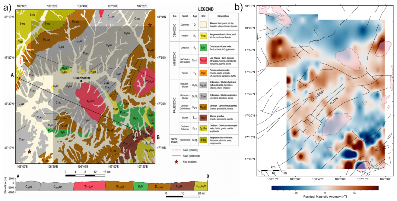
Figure 2.
Magnetic anomaly and derivative maps of the Ulaanbaatar region. (a) Reduced-to-pole (RTP) magnetic anomaly. (b) Analytic signal amplitude. (c) Total horizontal gradient (THG). (d) Tilt derivative (TDR). Black lines show mapped faults, and semi-transparent pink polygons indicate mapped granitoid bodies. White areas indicate regions outside the ground magnetic survey coverage.
Figure 2.
Magnetic anomaly and derivative maps of the Ulaanbaatar region. (a) Reduced-to-pole (RTP) magnetic anomaly. (b) Analytic signal amplitude. (c) Total horizontal gradient (THG). (d) Tilt derivative (TDR). Black lines show mapped faults, and semi-transparent pink polygons indicate mapped granitoid bodies. White areas indicate regions outside the ground magnetic survey coverage.
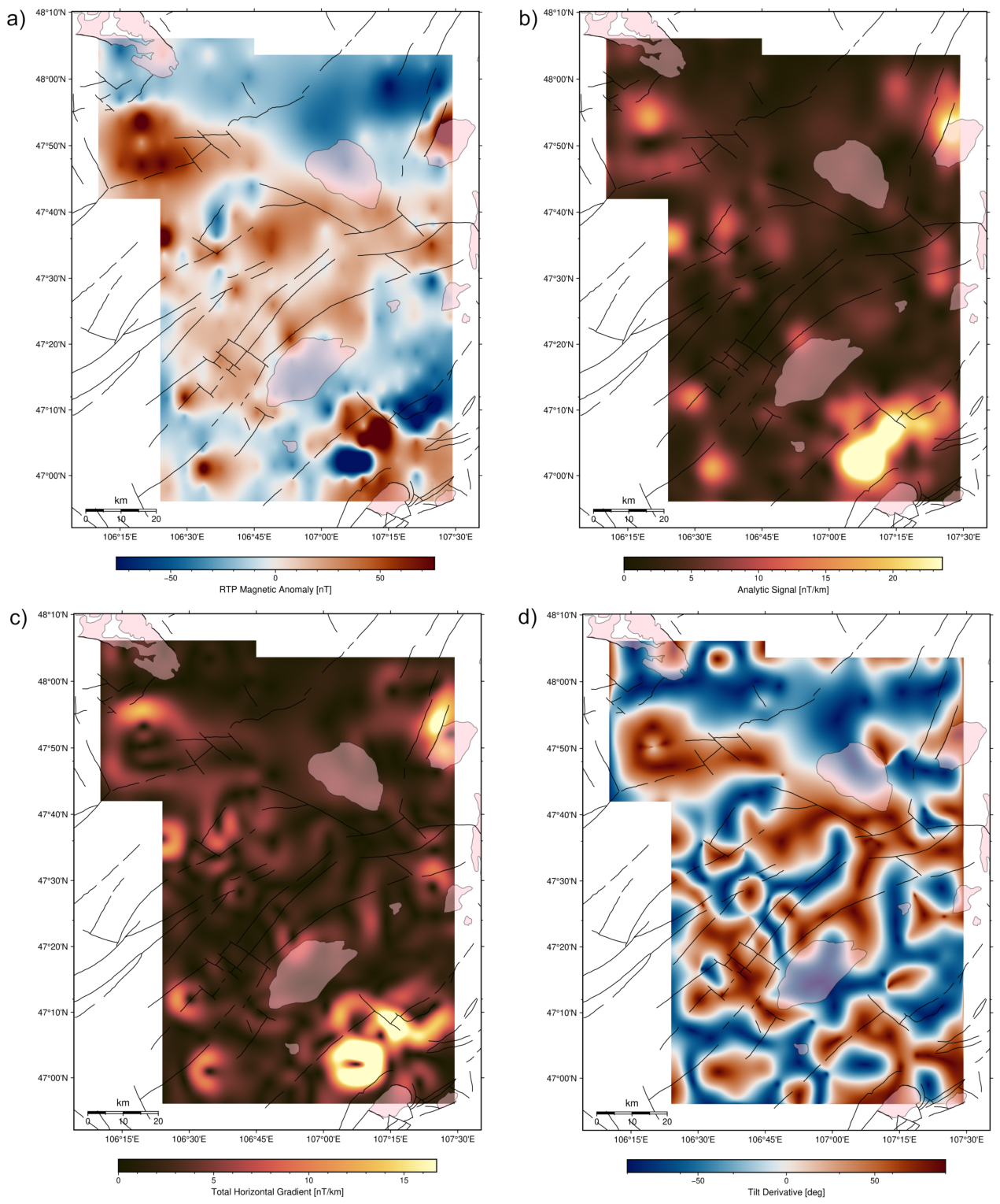
Figure 3.
Representative radially averaged magnetic spectrum and linear fits used for source–depth estimation. The high–wavenumber fit to gives km, whereas the lower–wavenumber fit to gives km; the estimated basal parameter is km.
Figure 3.
Representative radially averaged magnetic spectrum and linear fits used for source–depth estimation. The high–wavenumber fit to gives km, whereas the lower–wavenumber fit to gives km; the estimated basal parameter is km.
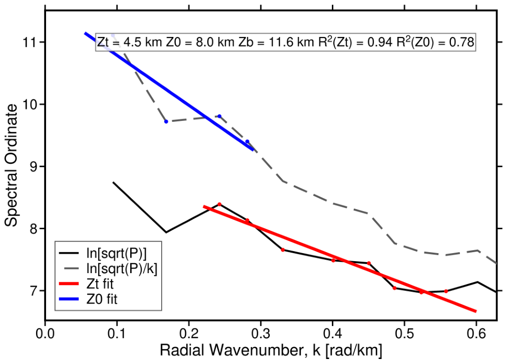
Figure 4.
Spatial distribution of magnetic source-depth estimates obtained from spectral analysis. (a) Top depth (), (b) centroid depth (), and (c) derived basal depth (). Black lines show mapped faults, and semi-transparent pink polygons indicate mapped granitoid bodies.
Figure 4.
Spatial distribution of magnetic source-depth estimates obtained from spectral analysis. (a) Top depth (), (b) centroid depth (), and (c) derived basal depth (). Black lines show mapped faults, and semi-transparent pink polygons indicate mapped granitoid bodies.
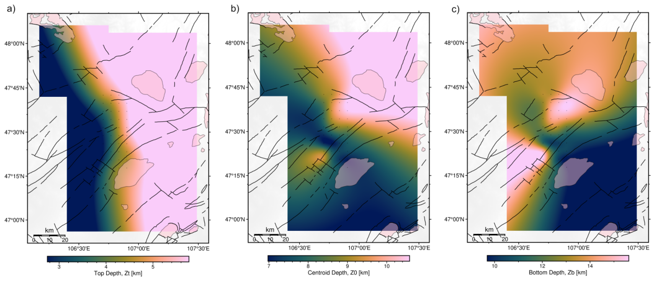
Figure 5.
Data fit for the three-dimensional magnetic susceptibility inversion. (a) Observed corrected residual total-field magnetic anomaly, (b) predicted response of the recovered model, and (c) observed-minus-predicted residuals. (d) Observed versus predicted anomalies. (e) Residual distribution and (f) normalized residual distribution. The final model yields an RMS residual of 2.59 nT, , , and NRMS = 0.49.
Figure 5.
Data fit for the three-dimensional magnetic susceptibility inversion. (a) Observed corrected residual total-field magnetic anomaly, (b) predicted response of the recovered model, and (c) observed-minus-predicted residuals. (d) Observed versus predicted anomalies. (e) Residual distribution and (f) normalized residual distribution. The final model yields an RMS residual of 2.59 nT, , , and NRMS = 0.49.
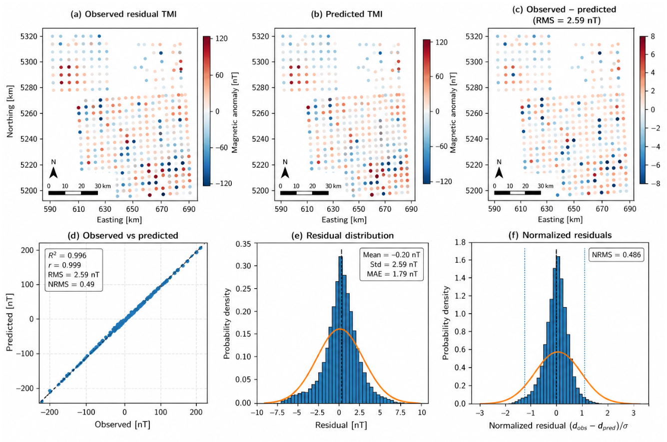
Figure 6.
Horizontal slices through the recovered three-dimensional magnetic susceptibility model at depths of 0, 2, 4, 6, 8, 10, 12, 14, and 16 km. Susceptibility is shown in SI units. Black lines indicate mapped faults, and semi-transparent polygons show mapped granitoid bodies.
Figure 6.
Horizontal slices through the recovered three-dimensional magnetic susceptibility model at depths of 0, 2, 4, 6, 8, 10, 12, 14, and 16 km. Susceptibility is shown in SI units. Black lines indicate mapped faults, and semi-transparent polygons show mapped granitoid bodies.
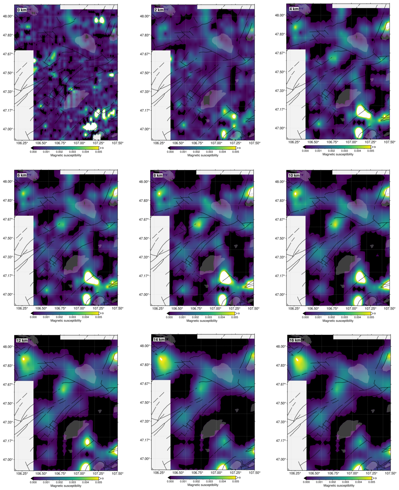
Figure 7.
Vertical sections through the recovered three-dimensional susceptibility model. Left panels show east–west sections at selected UTM northings, and right panels show north–south sections at selected UTM eastings. Susceptibility is shown in SI units.
Figure 7.
Vertical sections through the recovered three-dimensional susceptibility model. Left panels show east–west sections at selected UTM northings, and right panels show north–south sections at selected UTM eastings. Susceptibility is shown in SI units.
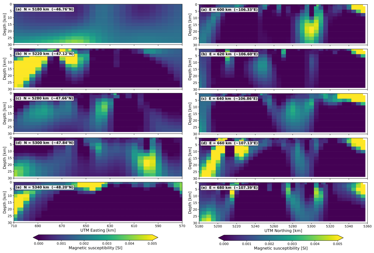
Figure 8.
Relationship between active faulting and subsurface magnetic structure in the Ulaanbaatar region. The left panel shows the horizontal susceptibility-gradient magnitude at 6 km depth with mapped active faults and inset rose diagrams comparing fault strikes with nearby magnetic-boundary orientations. The right panels show gradient- and susceptibility-enrichment ratios relative to the local 5–20 km background. Ratios greater than unity indicate preferential association with enhanced gradients along with susceptibility.
Figure 8.
Relationship between active faulting and subsurface magnetic structure in the Ulaanbaatar region. The left panel shows the horizontal susceptibility-gradient magnitude at 6 km depth with mapped active faults and inset rose diagrams comparing fault strikes with nearby magnetic-boundary orientations. The right panels show gradient- and susceptibility-enrichment ratios relative to the local 5–20 km background. Ratios greater than unity indicate preferential association with enhanced gradients along with susceptibility.
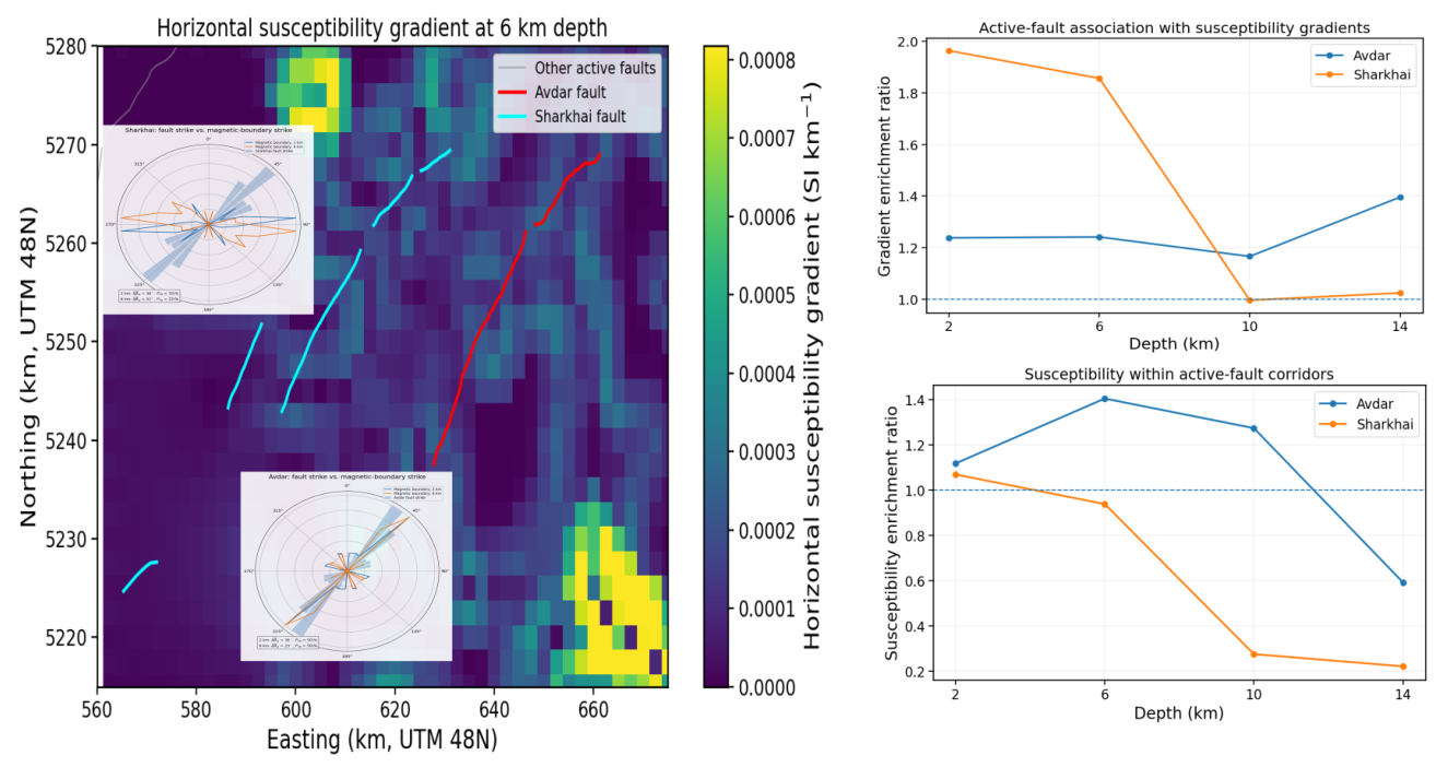
Figure 9.
Integrated representation of the magnetic architecture beneath the Ulaanbaatar region. The upper surface shows the residual total-field magnetic anomaly with mapped faults and granitoid bodies, whereas the vertical panel shows a representative section through the recovered susceptibility model. White lines show representative spectral source-depth levels ( km, km, and km) and do not represent discrete geological interfaces.
Figure 9.
Integrated representation of the magnetic architecture beneath the Ulaanbaatar region. The upper surface shows the residual total-field magnetic anomaly with mapped faults and granitoid bodies, whereas the vertical panel shows a representative section through the recovered susceptibility model. White lines show representative spectral source-depth levels ( km, km, and km) and do not represent discrete geological interfaces.
Disclaimer/Publisher’s Note: The statements, opinions and data contained in all publications are solely those of the individual author(s) and contributor(s) and not of MDPI and/or the editor(s). MDPI and/or the editor(s) disclaim responsibility for any injury to people or property resulting from any ideas, methods, instructions or products referred to in the content. |
© 2026 by the authors. Licensee MDPI, Basel, Switzerland. This article is an open access article distributed under the terms and conditions of the Creative Commons Attribution (CC BY) license (http://creativecommons.org/licenses/by/4.0/).
Copyright: This open access article is published under a Creative Commons CC BY 4.0 license, which permit the free download, distribution, and reuse, provided that the author and preprint are cited in any reuse.