

Submitted:
04 September 2026
Posted:
07 September 2026
You are already at the latest version
Abstract
The automated detection of surface defects on roads can help make condition assessments and develop maintenance plans as it allows road images to be transformed into machine-readable and localized data. The current research sets up a methodology for object detection and checks its performance for the detection of three surface categories: potholes, cracks, and manholes. The authors make sure that this research is considered as an empirical case study using a standard YOLOv8s detector rather than trying to prove a new detection method. The authors run the notebook acquiring our Road Damage Dataset which consists of 2009 manually labeled images and 4737 boxes in YOLO format. They produce a tidy bounding box table to guarantee the proper auditing of the dataset and conduct the necessary exploratory data analysis considering class balance, normalized geometry of the bounding box, spatial distribution of instances, co-occurrences of classes, image resolution, and constructed samples. Since the source dataset contains no validation collection in the notebook, a random selection of 15% images amounting to 302 images was held out, the detector achieves an overall precision of 0.921, recall of 0.877, mAP@0.50 of 0.953, and mAP@0.50:0.95 of 0.652. Manhole detection is strongest in mAP@0.50 (0.974), while crack detection provides the highest recall (0.895). Potholes are comparatively more difficult, with recall of 0.828 and mAP@0.50:0.95 of 0.607. The experiment demonstrates that a compact, pretrained one-stage detector can provide strong baseline performance on this three-class road-damage dataset. The results also expose important research limitations: the holdout is derived from the same original collection, no independent external test set is used, and no detector baseline or ablation study is reported. These limitations motivate future work on external validation, class-imbalance handling, detector benchmarking, and deployment-oriented evaluation.
Keywords:
road damage detection
; pothole detection
; crack detection
; manhole detection
; object detection
; YOLOv8s
; computer vision
; deep learning
; infrastructure monitoring
; road-surface inspection
1. Introduction
The deterioration of road surfaces is a chronic problem that affects infrastructure as defects have implications on ride quality, safety, drainage, maintenance expenditure, and the timing of remedial action. Conventional inspection programs typically use manual visual surveys or specialized sensor technology to achieve their objectives and this creates operational challenges in cases where road networks are vast and changing from time to time or where they are dispersed across great distances. Image-based computer vision represents a new approach whereby roads are photographed and images of roads can yield information on the location and type of defects. Initial studies involving deep-learning have confirmed that the damage to the road can be established from images taken from mobile phones or cameras mounted on moving vehicles [1].
With an increase in datasets in terms of size and geographical direction, the task of road-damage recognition has also moved from image classification to object detection, where different damage can be located by means of a bounding box. Maeda and co-authors [1] demonstrated that it is indeed possible to detect multiple cases of road damage based on images taken by smartphones, and the RDD2022 benchmark took the issue on a large scale in terms of the number of images (47,000) collected in six countries altogether [2]. The importance of the above-mentioned findings cannot be underestimated since one type of road damage may differ from the other quality-wise. In small cracks, the damaged piece of road may be extremely long and narrow, whereas potholes can occupy irregularly-shaped areas. The resulting systems should learn semantic category and spatial extent at the same time rather than rely entirely on the general image.
The dataset utilized in the study at hand has recently made headlines as a real-world road defect dataset containing 2,009 hand-labeled images taken in several areas of Rome and its surrounding semi-urban and rural sites, comprising three main classes—potholes, cracks, and manholes/manholes [3]. The usefulness of this dataset rests on the fact that three classes can be present in the same frame and its images can have realistic conditions and viewpoints. The notebook that has been obtained includes 4,737 bounding boxes within these 2,009 images, where cracks account for the biggest share of annotated cases. This disbalance is a highly important thing to take into consideration as such disbalance can create obstacles for optimization and lead to the situation when the detector “learns” the major visual models more efficiently than the less represented classes.
For the purpose of detecting objects, one-stage detectors are appealing because they allow the same model to identify varying items at once while having quite a smooth inference pipeline. Originally, YOLO employed to transform detection into the simplest regression from images to bounding boxes and class probabilities thus allowing for prediction to be implemented within a network in an end-to-end way. At the same time, later studies into detecting systems revealed the importance of multi-scale feature representations for various objects due to their different dimensions and dimensions with Feature Pyramid Networks providing its users with a more scientific way of integrating the semantic information across the different resolutions [5]. These investigations can be directly applied to the road pictures since for the purposes of defining a crack a very small part of the image will be necessary while defining a pothole or relaxing outdoor bath will most probably require more sophisticated means of solving the issue.
Hence, this research investigates the practicality of YOLOv8s in solving the road-damage problem at hand. The aim is not to come up with another architecture, loss function, attention mechanism, or detection head. Rather, the study intends to record the entire experiment involving datasets gathering and parsing, exploratory analysis, data exclusion, model training, evaluation, etc. The value of such a transparent baseline is that it helps introduce measurable references points before any further complicated developments are undertaken.
Besides, the study is motivated from a data-driven perspective, since before training data is analyzed through class frequency plots, bounding box area and aspect ratio distributions, spatial density maps, co-occurrence matrices, image resolution summaries and annotated mosaics. This is crucial, as the statistical and geometric characteristics of the data can help uncover problems that cannot be identified using the overall accuracy measure alone. For instance, the class balance ratio observed here is equal to 2.63 for the most frequent and the least frequent classes and all pictures in the collection have the same original resolution, which equals 640 × 360 pixels. Thus, subsequent model training is performed using 640-pixel data inputs, providing the necessary standardized representation for the detector while keeping the original visual content of the images intact.
Using this foundation, the work makes three valuable contributions. To start, it offers a reproducible depiction of an end-to-end YOLOv8s baseline in a three-class road-damage dataset. Next, it describes the dataset structure and provides relevant object-level statistics in terms of the executed notebook with 2,009 images, 4,737 labeled observations, 302 images, and 728 holdout observations. Finally, it delivers a comprehensive study of general and class-specific detection performance, with evidence from the training curves, confusion matrix, metric summaries, and qualitative results.
2. Related Work
Road damage detection has transitioned from having to rely on manual processes of image processing to utilizing deep neural networks that learned powerful visual representations from huge collections of road images. Maeda et al. [1] became one of the first to demonstrate the use of large-scale deep learning with smartphones, showing the ability to implement detection and classification in the context of operational inspection workflow. This work was important as it demonstrated how road damage can be treated as a machine learning problem by utilizing standard images instead of expensive acquisition devices.
The introduction of big public datasets made it possible to conduct more extensive evaluations. Authors Arya and others [2] created the RDD2022 data set that includes pictures from Japan, India, the Czech Republic, Norway, the USA, and China and four types of damage typing. The multi-country nature of the RDD2022 data set raised the issue concerning the changes in the appearances of road defects: camera type, road material, climate, traffic, and road maintenance can influence the appearance of the defect. A more recent three-class dataset used in the study contributes to the development of the three-class pothole, crack, and manhole dataset [3].
From the point of view of detector design, YOLO created a paradigm in which localization and classification happen simultaneously directly from an entire image [4]. YOLOv2 advanced this idea further through numerous architectural and training improvements such as multi-scale training and proved that Y OLO-related architectures are effective in practical cases where a balance between speed and precision must be achieved [6]. Furthermore, YOLOv4 continued this developmental idea by systematically implementing all the training and architectural advancements accomplished earlier, including cross-stage partial connections, mosaic augmentation, and localization advancements connected to CIoU [7]. All these developments explain why YOLO-type detection devices are still of great importance for practical needs.
Recent research in real-time detection has sought to pursue the accuracy-efficiency frontier. YOLOv7 has exhibited strong performance over a wide range of speeds and highlighted trainable bag-of-freebies for achieving good efficiency for detectors [8]. At the same time, two-stage methods such as Faster R-CNN are still relevant models because their Region Proposal Network generates proposals for potential target positions before the actual classification and refinement stages [9]. Similarly, single-shot methods like SSD skip proposal generation phase and leverage multiple feature map resolutions to detect objects across different scales [10].
The previous research gives the methodological background for assessing the current notebook experiment. The study uses a YOLOv8s model because it matches the YOLO format of the dataset annotations as well as provides an effective baseline for the single-stage detection approach. Unlike other comparative studies that explore multiple architectures in controlled conditions, the notebook contains only a single trained detector. Therefore, it can be concluded that the main contribution of the present manuscript is the transparency and reproducibility of the baseline experiment and not the argument that YOLOv8s is superior to all alternative detectors.
The literature also puts forward various ways to improve the present research. The use of cross-dataset validation can help check generalizability while multi-scale training may assist in cases where a defect varies widely in size. Several class balancing methods can help in the cases when certain classes dominate the rest. Conducting controlled comparisons can help uncover the accuracy vs computational expense trade-off. Therefore, the current research results should be seen as practically the first milestone when it comes to understanding the strengths and weaknesses of the current approach.
3. Methodology
The methodology is based on the developed notebook as a serial but analysis-based process. The workflow starts from dataset collecting and annotation analysis, continues to object-focused exploratory analysis, creates a validation set that is hold-out, adjusts the pre-trained YOLOv8s detector, and finishes with quantitative and qualitative evaluation. The overall methodology scheme is shown in Figure 1.
3.1. Dataset and Data Acquisition
Through KaggleHub, the notebook retrieves the dataset using the dataset slug for the Road Damage Dataset which consists of images of manholes, cracks, and potholes. The overall collection consists of 2009 images, where each one has YOLO-style annotations that are recorded in rows containing the variables class_id, x_center, y_center, width, height. The values indicated in the rows are in the range between 0 and 1. During the experiment, the classes that were used are: class 0 = pothole, class 1 = crack, class 2 = manhole.
Table 1 below indicates the dataset profile taken straight from the notebook. Class totals comprise 1,261 potholes, 2,519 cracks, and 957 manholes, which makes a total of 4,737 bounding boxes. Cracks also make approximately 53.18% of the entire labeled instances, while potholes take up 26.62%, and manholes 20.20%.
3.2. Annotation Parsing and Object-Level Representation
Within the notebook a neat dataframe is created in which each labeled object refers to one row in the dataframe. OpenCV provides pixel dimensions from raw photos, while normalized YOLO coordinates are kept as well. In addition to original normalized coordinates, different metrics have been computed such as normalized area, approximate pixel area, absolute width and height of the bounding box, image dimensions and image metadata. This so-formed representation brings about the possibility to aggregate information without repeated reading of the raw label files.
For an image of width W and height H, the YOLO representation (x_c, y_c, w_b, h_b) can be converted into pixel coordinates as follows:
x_1 = W (x_c - w_b / 2), y_1 = H (y_c - h_b / 2)
x_2 = W (x_c + w_b / 2), y_2 = H (y_c + h_b / 2)
A_n = w_b h_b, A_p = w_b h_b W H
In this equation A_n represents a normalized box area equivalent to an image area while A_p is approximated pixel area corresponding to this box area. These quantities are useful for creating exploratory graphs for analyzing geometrical characteristics of the defects. This is especially useful for road images because elongated cracks and compact manholes can lead to dissimilar width to height and area distributions regardless of the number of pixels occupied in the two cases.
3.3. Exploratory Data Analysis
The purpose of the notebook’s exploratory data analysis is to provide clarity around the characteristics of the dataset prior to training a model. Such an analysis entails aspects like the frequency of each class, distribution of the box areas across images, values of the aspect ratios, densities of the spatial centers of the boxes, number of boxes per image, co-occurrences of classes within an image, and a sample (mosaic of images) providing the distribution of the image resolution across the dataset. These analyses are not another version of prediction but provide a means for collecting descriptive information with regard to the problems of imbalance, geometry, and structure of the datasets.
The left panel shows that there are 1,261 potholes, 2,519 cracks, and 957 manholes. The right panel illustrates how the class distribution is the same in the collection being studied. Figure 2 demonstrates a noticeable imbalance between classes. Cracks dominate the others, having twice as many instances of potholes and having a particularly high number of instances for manholes. There was a ratio of maximum to minimum instances equal to 2.63. The imbalance is significant because it means that the detector were exposed to a lot of instances of the cracks category and thus might build better decision boundaries for cracks category than for minority classes.
covering normalized area distributions, class-specific aspect ratios, spatial box-center density, and distribution of boxes in an image. The data audit is expanded in Figure 3 from class counts. The normalized area distribution gives the scale of the annotated objects with respect to the source image, and the aspect ratio plot shows differences in shapes. The spatial density plot shows the locations of the centers of the boxes on the normalized image, thus giving information about viewpoint and composition of the scene. The histogram of boxes per image gives information about the degree of multi-instance content, which is important since the detector has to be able to distinguish between multiple defects in the same road frame.
Figure 3.
Bounding-box geometry analysis.
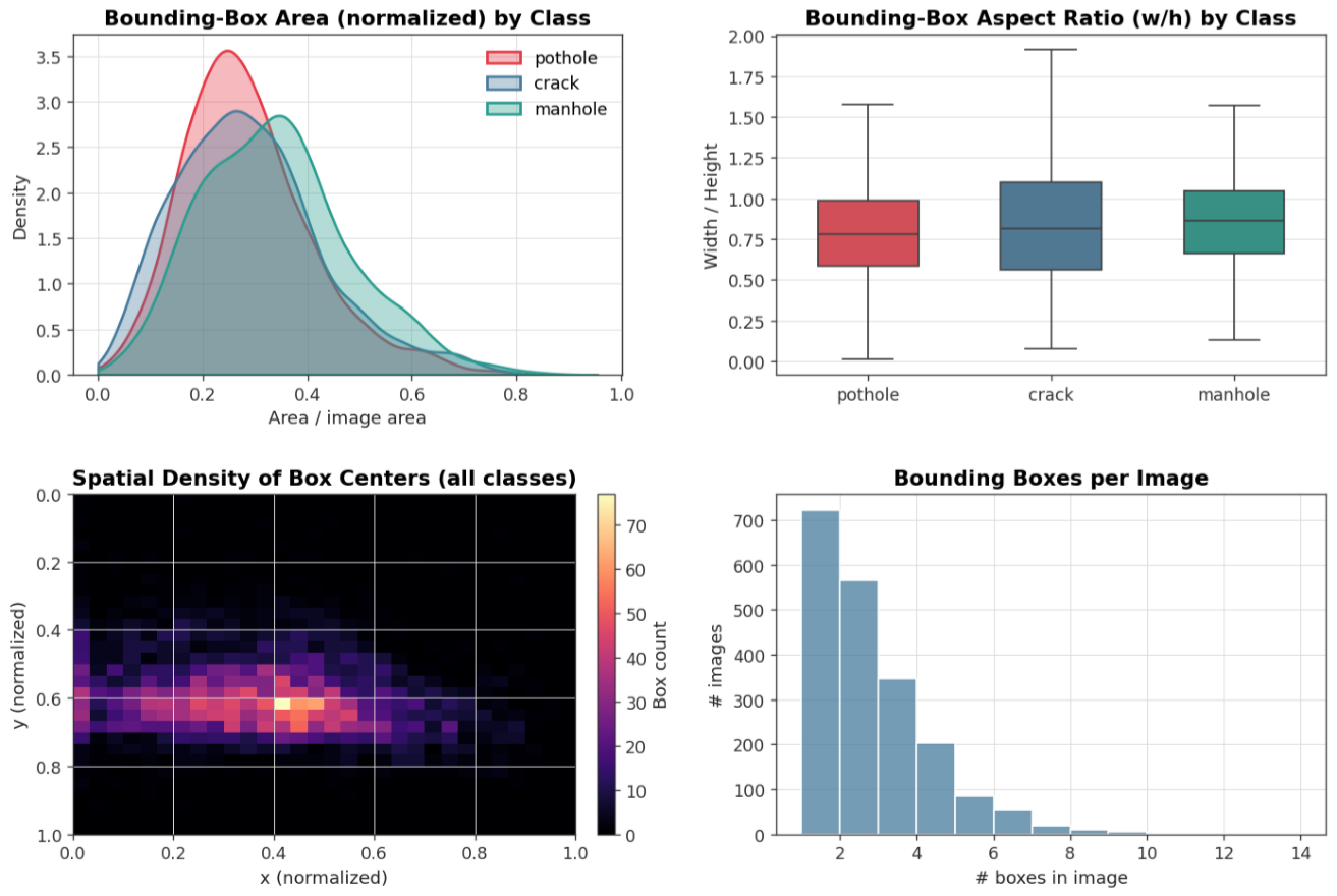
Figure 4.
Class co-occurrence and image-resolution analysis.
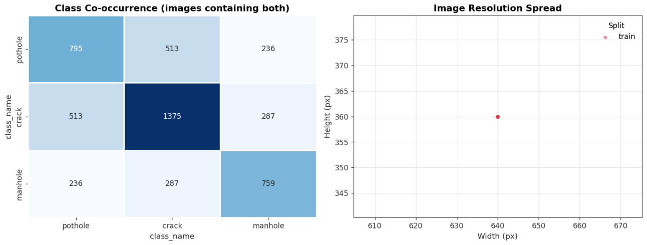
The co-occurrence matrix indicates how many images include each combination of class, while scatter plot demonstrates the native resolution distribution. Co-occurrence calculation indicates presence, not counts. In other words, an image has one contribution. Then co-occurrence matrix will be generated from multiplication of matrices. Co-occurrence analysis shows how damage classes co-occur, suggesting that detector should be trained regardless of classes mixed in one image. Besides, resolution analysis is important to assure repeatability of results. The notebook states that only one unique source resolution was found and the image has 640×360 px resolution, which means no variability of native resolution in the database.
Figure 5.
Annotated sample mosaic.
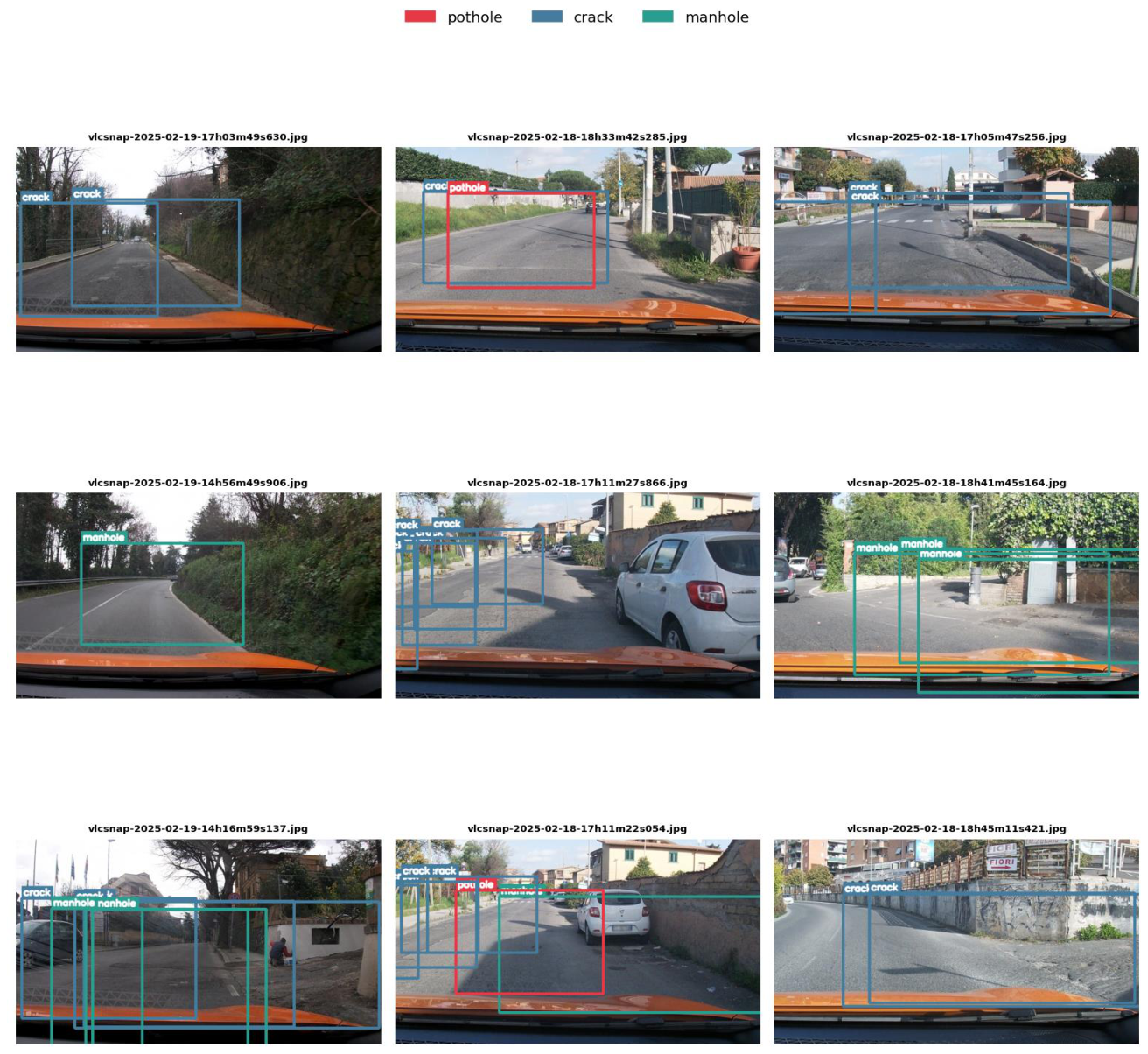
Ground-truth YOLO bounding boxes were superimposed onto representative dataset images for a visual inspection of label quality and scene variation.The sanctioned mosaic serves as a qualitative sanity check for the labeled images rather than relying on numeric summaries alone, thus allowing the experimenter to confirm whether bounding boxes match visible road objects and whether class labels are associated in a consistent manner. Such inspection is important prior to training since an annotation problem can otherwise be mistaken for a model shortcoming.
3.4. Validation Holdout Construction
The program does not identify a given directory structure for training, testing or validation purposes. As a result, it proceeds to create a writable data configuration for YOLO. It also realizes that only the folder for training is available, so it uses scikit-learn train_test_split with a fixed random state to reserve 15% of the total number of images for validation. A total of 302 images are allocated for validation, while the rest of the images remain in the training set. Of interest is the fact that the split is done at image level and randomly. Thus, the split at hand is not done with respect to classes.
The table provides an experimental split that has been made based on the workflow from the notebook. In the holdout there are 197 instances of potholes, 391 instances of cracks, as well as 140 instances of manholes. Since the holdout comes from the original data set, we still need a separate external test set.

Table 2.
Image-level partition used by the notebook.
| Split component | Images | Instances | Role |
| Original indexed corpus | 2,009 | 4,737 | Training source collection |
| Random holdout | 302 | 728 | Validation/evaluation split |
| Remaining training pool | 1,707 | 4,009 | Model fine-tuning pool |
3.5. YOLOv8s Training Procedure
The trained detector takes the pretrained yolov8s.pt checkpoint as a starting point and is subjected to fine-tuning for the three target classes. In this notebook, Ultralytics 8.3.253 is used during the recorded run; a Tesla T4 GPU is employed, the maximum number of epochs is 80, the input size is 640 pixels, the batch size is 16, a fixed random seed and early-stopping patience of 15 epochs are applied. Optimizer =“auto” is employed and the recorded optimizer configuration is AdamW with the automatically selected learning rate of around 0.001429 and the momentum value of 0.9. Weight decay is applied with the help of optimizer parameter groups. The configurations described above are reproduced here since training settings influence both convergence and reproducibility of provided metrics.
In Table 3 of the report, the YOLOv8s training configurations derived from notebook execution have been showcased. We can think of detector as a mechanism that links input images (I) to output detections (D = {(b_i, c_i, s_i)}, where b_i is a predictor for the object bounding boxes, c_i is a predictor for object classes, and s_i is the success rate of prediction. The training approach relies on upward optimization improving prediction accuracy and localization thanks to the relevant YOLOv8 concepts employed by Ultralytics. This paper does not describe any unknown previous loss metrics necessary for presenting particular experiments; the only information provided here is related to results achieved in the course of all the tests made.
4. Results
The outcomes are presented in three distinct phases: training dynamics, average validation performance, and class-wise behavior. The evaluation of the model is done using the 302-image holdout created as explained in section. The version of model used for qualitative evaluation is best.pt which is obtained from the training process.
The training losses, validation losses, and validation metrics from results.csv have been replotted in the notebook in a publication-friendly format. In Figure 6, a convergence-oriented insight of the experiment can be seen. Showing how the losses diminish, the loss panels show the changes in training and validation goals of the detector over epochs, whereas the metric panel illustrates changes in precision, recall, mAP@0.50, and mAP@0.50:0.95. Rather than viewing the figure in isolation, it should be interpreted in conjunction with the final validation results table since the key objective of the curves is to evaluate if the model improves consistently and if validation results are in line with training outcomes.
4.1. Evaluation Metrics
The efficiency of object detection relies on accuracy in classification and localization. The notebook also mentions precision, recall, mAP@0.50 and mAP@0.50:0.95. According to the IoU threshold τ, the intersection over union of the predicted box B_p and the actual box B_g would be defined as:
IoU(B_p, B_g) = |B_p ∩ B_g| / |B_p ∪ B_g|
According to the evaluation method of the detector, the overlap is considered to be a successful localization if the relevant criterion under the IoU is fulfilled. Precision and recall measure the balance between correct detections, unsuccessfully detected objects and falsely identified objects:
Precision = TP / (TP + FP)
Recall = TP / (TP + FN)
F1 = 2 × Precision × Recall / (Precision + Recall)
Average Precision (AP) gives a detailed account of the relationship between precision and recall for a given class at a particular level of IoU. Mean Average Precision (mAP) is defined as the average of AP values across various classes. In this paper, mAP@0.50 is the average AP at IoU = 0.50, while mAP@0.50 to 0.95 means the stricter average calculated from IoU values between 0.50 to 0.95 according to the Ultralytics evaluation protocol. The difference between the two provides essential information that indicates that the detector may provide correct detection of an object at a modest overlap level but may have lower localization accuracy at stricter levels of overlap.
4.2. Overall and Per-Class Performance
In terms of accuracy, the overall precision of 0.921 suggests that most boxes predicted are quite accurate under the assessment guidelines while the recall of 0.877 signifies that a smaller but significant proportion of identified objects remain unidentified. The mAP value of 0.953 implies that the performance of overall class is good according to a moderate threshold of overlap. The lesser mAP, which is the mAP@0.50:0.95 at 0.652, is rightly attributed to a more stringent localization requirement. The detector is accurate in identifying the right objects; however, the margins of the predicted block are not consistently rigid to reflect the same success of detection at higher IoU thresholds.
Table 4 presents the ultimate validation results obtained through YOLOv8s evaluation. The row titled “Combined” displays the overall figures calculated across the 302-image, 728-instance dataset. Nonetheless, class-specific figures disclose more significant results. The manhole class is the easiest one in the dataset based on scores of mAP@0.50 (0.974), precision (0.963), and recall (0.907). The crack class achieves the highest recall rate (0.895), which is especially important as it is the class with the highest frequency in the dataset. On the other hand, potholes have the lowest recall (0.828) and the lowest mAP@0.50:0.95 (0.607), indicating that the model either does not detect potholes and/or does not draw their borders accurately. Such statistics demonstrates the imbalance of the dataset and caters to the shapes variability of the problem pointed out during EDA even though the notebook does not comprise a controlled ablation.
In conjunction with the metrics used for describing detection accuracy, Figure 7 depicts the distribution of correctly detected objects, missed objects, and background errors in a confusion matrix, in addition to presenting the comparison of the number of detections per class. This figure is an effective way of determining whether there is any category that systematically does not perform well. In this experiment, the bar graph supports the observation made earlier that the recall for potholes is lower than for cracks and manholes, while manhole precision and mean average precision at IoU equal to 0.50 is the highest for these three classes.
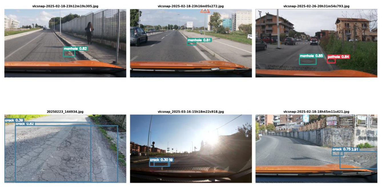
The qualitative gallery offers a visual verification of the performance of the detector on the reserved images. While quantitative metrics give general data, visual inspections reveal if the detector finds defects in plausible areas and whether it offers reasonable predictions of their corresponding confidence scores. However, it is crucial to understand that this gallery is not to be used as a replacement for quantitative evaluation since only a limited sample is provided; its function is to demonstrate that the detector creates reasonable localizations of defects in realistic traffic situations.
Figure 7.
Confusion matrix and class-wise precision.
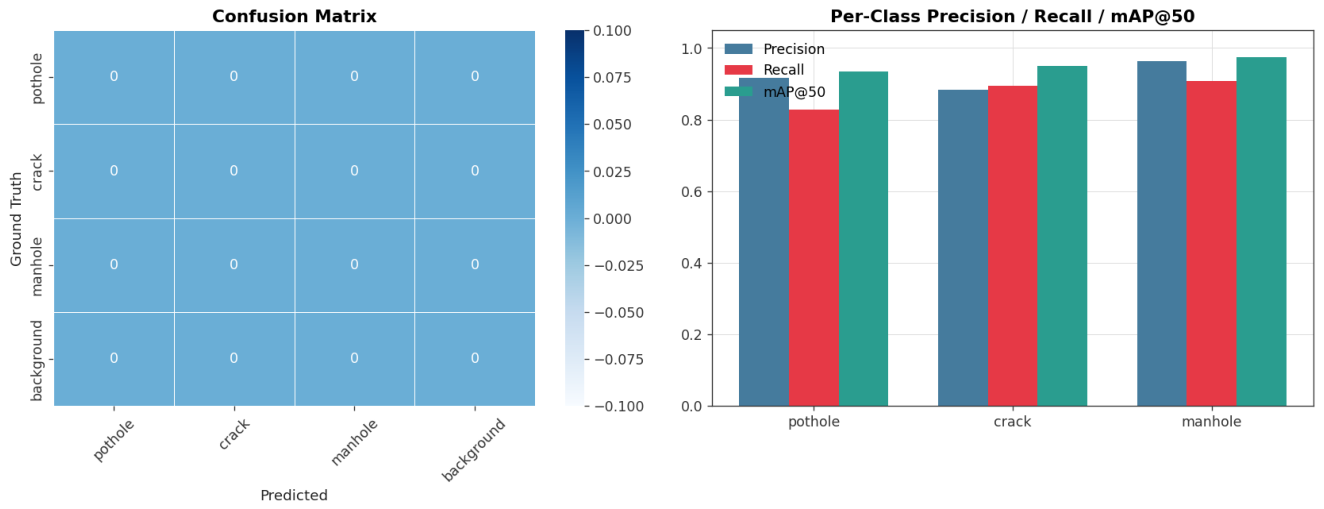
Figure 8.
Qualitative inference gallery.
5. Discussion
The test shows that YOLOv8s can provide a good baseline for the detection of the road surface of three classes when using the annotations that were provided. The overall mAP@0.50 of 0.953 and precision of 0.921 shows that the detector can identify and properly localize the necessary classes according to the evaluation conditions established in this notebook. The performance in recognition of the manholes is very promising, given that precision and recall are both higher than 0.90. In practical terms, it means that a single-stage detector is able to turn regular road images into localizations of possible defects, ready for further inspection. The actual mAP@0.50:0.95 score of 0.652 is significantly lower compared to the mAP@0.50 result, which shows that the localization task is more challenging when using stricter criteria to measure the overlap. This difference is important for road inspection since the maintenance decisions will be made not only based on the fact that the defect is identified but also its localization and size because of that. Thus, the optimization process needs to be directed toward improvement of localization quality instead of the easy task of achieving 0.50-IoU result only.
The pattern which is determined by classes of defects is also valuable. Cracks are the dominant defect class and have very good recall in line with how many examples of defects are available to detect the cracks. Potholes belong to the smaller set of defects of the two bigger ones, but have low recall and low mAP. Manholes are rare but still can be detected very well, which means that the eye-catching novelty of the defect can alleviate the issue of obtaining enough samples. However, given the fact that the notebook does not include any controlled rebalancing experiments, these statements should remain assumptions rather than causal statements. A technical limitation seen here is related to the experiment protocol. The dataset is used as one set containing 2,009 images, with the notebook using 302 images for validation purposes later. This is ok for this kind of study but does not mean that the tests have been done on an independent dataset that was gathered in different conditions. Given this fact, the metrics reported can be considered as optimistic while applying them to real applications. The research is also without a baseline control comparison. With no second detector, it cannot be proven that YOLOv8s is superior, faster or more efficient compared to Faster R-CNN, SSD, some YOLO version or a light-weight deployment model. Moreover, there is no ablation for class balancing, augmentation and input resolution. The current paper should thus be presented as an empirical baseline study where the major contribution is reporting on the data pipeline and the observed performance rather than claiming to use a state-of-the-art model.
The notebook records various data on computational performance only partially. According to the validation procedure, it requires around 0.6 ms for preprocessing, 5.4 ms for inference, and 0.8 ms for post-processing per image on the Tesla T4. These data show that the GPU inference could be efficient in the current setup, but the results can’t be extended to edge devices, CPUs, and embedded systems without proper testing. The study designed to report the deployment results must describe latency, memory demand, model size, energy consumption, and accuracy indicators. The main limitation of the study is the lack of an independent external test set since 302 evaluation images are taken from one collection, and there is no independent proof for geographic, shooting device, and scene generalizability. The second limitation is the class imbalance since cracks constitute 2,519 out of 4,737 data points. Third, the experiment evaluates only YOLOv8s, preventing comparative conclusions about architecture choice. Fourth, the random holdout is not class-stratified, which can introduce sampling variability in the class composition of the validation split. Fifth, the notebook does not provide uncertainty estimates or repeated-run variance, so the reported metrics represent one fixed training/evaluation run rather than a distribution over multiple seeds.
To sum up, the prospects of future research should concentrate on five areas of experimental advancements (1) testing on a previously unseen external dataset or independently collected image data; (2) comparing the performance of YOLOv8 with other YOLO models of all sizes and with at least one two-stage detector; (3) investigating the effect of oversampling, class-aware augmentation, or loss weight adjustment for minority classes in the dataset; (4) performing multiple iterations or cross-validation in order to gain a better understanding of the variability of the metrics obtained in the experiment; (5) evaluating the performance in the field of application, taking into account the speed and memory. In particular, an interesting instance of future research could be conducting an experiment on the effect of input resolution and augmentation used on the efficiency of the detector in identifying small or long cracks.
6. Conclusions
This manuscript proposes a thorough and reproducible foundation for the identification of potholes, cracks, and manholes through the images of roads obtained by YOLOv8s. The work is carried out according to the executed notebook starting from the collection of the required data and finishing off with comprehensive exploratory analysis involving random holdout establishment, fine-tuning of the pretrained model, as well as quantitative and qualitative evaluation. As a result, the final detector achieves indices of 0.921 precision, 0.877 recall, 0.953 mAP@0.50, and 0.652 mAP@0.50:0.95 on 302-image holdout containing 728 instances that have been labeled. The best detection is achieved in terms of manhole detection, the recall of cracks is the highest, and pothole detection is the biggest challenge in the process of improvement. Thus, the main contribution of the present paper is said to be an empirical baseline rather than a new approach in detection systems. In addition, the results of the present research reveal that an ordinary one-stage detection system can really work well with the above-mentioned three-class dataset, although it must be emphasized that independent external validation, assessment of the system capabilities, solution of the inherent problem of imbalance and testing of the system for practical use should be conducted before going further steps with regard to operational systems of road inspections.
7. Reproducibility and Data Availability
The analysis is derived from the supplied road-damage notebook and its executed artifacts. The dataset is accessed in the notebook through KaggleHub using the public dataset slug for the Road Damage Dataset containing potholes, cracks, and manholes. The experiment uses Ultralytics YOLOv8s, OpenCV, pandas, NumPy, scikit-learn, Matplotlib, and Seaborn. Reproduction requires access to the same dataset version and a compatible Ultralytics environment; exact metric reproduction can also depend on the recorded random seed, software versions, and hardware.
Supplementary Materials
The following supporting information can be downloaded at the website of this paper posted on Preprints.org.
References
- H. Maeda, Y. Sekimoto, T. Seto, T. Kashiyama, and H. Omata, “Road Damage Detection and Classification Using Deep Neural Networks with Smartphone Images,” Computer-Aided Civil and Infrastructure Engineering, vol. 33, no. 12, pp. 1127–1141, 2018. [CrossRef]
- D. Arya et al., “RDD2022: A multi-national image dataset for automatic Road Damage Detection,” arXiv:2209.08538, 2022.
- L. Arcioni et al., “Real-world road damage dataset with potholes, cracks, and maintenance holes,” Scientific Reports, 2026. [CrossRef]
- J. Redmon, S. Divvala, R. Girshick, and A. Farhadi, “You Only Look Once: Unified, Real-Time Object Detection,” in Proc. IEEE CVPR, 2016, pp. 779–788. [CrossRef]
- T.-Y. Lin, P. Dollár, R. Girshick, K. He, B. Hariharan, and S. Belongie, “Feature Pyramid Networks for Object Detection,” in Proc. IEEE CVPR, 2017, pp. 2117–2125. [CrossRef]
- J. Redmon and A. Farhadi, “YOLO9000: Better, Faster, Stronger,” in Proc. IEEE CVPR, 2017, pp. 7263–7271. [CrossRef]
- Bochkovskiy, C.-Y. Wang, and H.-Y. M. Liao, “YOLOv4: Optimal Speed and Accuracy of Object Detection,” arXiv:2004.10934, 2020.
- C.-Y. Wang, A. Bochkovskiy, and H.-Y. M. Liao, “YOLOv7: Trainable bag-of-freebies sets new state-of-the-art for real-time object detectors,” arXiv:2207.02696, 2022.
- S. Ren, K. He, R. Girshick, and J. Sun, “Faster R-CNN: Towards Real-Time Object Detection with Region Proposal Networks,” in Advances in Neural Information Processing Systems, vol. 28, 2015.
- W. Liu et al., “SSD: Single Shot MultiBox Detector,” in European Conference on Computer Vision, 2016, pp. 21–37. [CrossRef]
Figure 1.
Methodological workflow.
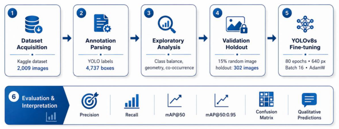
Figure 2.
Class distribution.
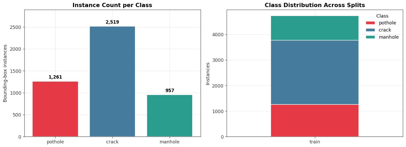
Figure 6.
Training and validation dynamics.
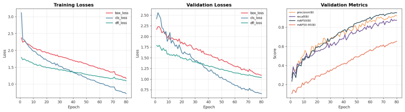
Table 1.
Dataset and annotation summary used in the experimental pipeline.
| Dataset property | Value | Interpretation | Source in notebook |
| Images | 2,009 | Complete indexed image collection | Cell 7 |
| Bounding boxes | 4,737 | All parsed object instances | Cell 7 |
| Classes | 3 | Pothole, crack, manhole | Cells 1, 5 |
| Native resolution | 640 × 360 px | Single unique resolution | Cell 12 |
| Mean boxes/image | 2.36 | Average annotated objects per frame | Cell 8 |
| Max/min class ratio | 2.63 | Crack-dominant class imbalance | Cell 10 |
Table 3.
Reproducibility-oriented training and evaluation configuration
| Training parameter | Notebook value |
| Model | YOLOv8s, pretrained yolov8s.pt |
| Maximum epochs | 80 |
| Input size | 640 × 640 |
| Batch size | 16 |
| Seed | Fixed seed defined in notebook |
| Patience | 15 epochs |
| Optimizer | AdamW via optimizer=“auto” |
| Recorded LR | ≈ 0.001429 |
| Momentum | 0.9 |
| Device | Tesla T4 / CUDA:0 |
| Model size | 11,126,745 parameters; 28.4 GFLOPs |
Table 4.
Class-level YOLOv8s validation metrics for the three road-surface categories.
| Class | Images | Instances | Precision | Recall | mAP@0.50 | mAP@0.50:0.95 |
| All | 302 | 728 | 0.921 | 0.877 | 0.953 | 0.652 |
| Pothole | 120 | 197 | 0.916 | 0.828 | 0.933 | 0.607 |
| Crack | 204 | 391 | 0.884 | 0.895 | 0.950 | 0.675 |
| Manhole | 115 | 140 | 0.963 | 0.907 | 0.974 | 0.674 |
Disclaimer/Publisher’s Note: The statements, opinions and data contained in all publications are solely those of the individual author(s) and contributor(s) and not of MDPI and/or the editor(s). MDPI and/or the editor(s) disclaim responsibility for any injury to people or property resulting from any ideas, methods, instructions or products referred to in the content. |
© 2026 by the authors. Licensee MDPI, Basel, Switzerland. This article is an open access article distributed under the terms and conditions of the Creative Commons Attribution (CC BY) license (http://creativecommons.org/licenses/by/4.0/).
Copyright: This open access article is published under a Creative Commons CC BY 4.0 license, which permit the free download, distribution, and reuse, provided that the author and preprint are cited in any reuse.