
Submitted:
04 September 2026
Posted:
07 September 2026
You are already at the latest version
Abstract
Can data-driven learning move beyond approximating solutions of the prescribed PDE problems to constructing reusable numerical methods? We investigate this question through finite elements and develop a physics-informed hard-constrained manifold learning Finite Element (HCML-FE) framework. Physics-informed linear hard constraints on the element stiffness matrix are analytically transformed into algebraic relations among its entries. Symbolic Gaussian elimination then identifies the independent stiffness parameters and deterministic reconstruction operator. A neural-network predicts only these independent parameters, while the complete stiffness matrix is reconstructed analytically so that the prescribed linear mechanical constraints are satisfied exactly. For the four-node plane-stress and eight-node solid-shell elements considered here, only 3 and 78 independent stiffness parameters are required, respectively, to reconstruct the stiffness matrices. Their numbers and matrix locations remain unchanged over the admissible ranges of element geometry and material parameters. Reference data are obtained from independently developed finite-element programs and commercial finite-element software, allowing the framework to be examined using element technologies of different origins. Numerical results show that the HCML-FE passes rigid-body zero-energy and prescribed patch tests, reproduces characteristic element behaviors under locking, mesh distortion, and mesh refinement, and remains reusable and assemblable in complex two- and three-dimensional structures. These results demonstrate a data-driven route to numerical-method construction in which finite-element theory defines the admissible stiffness space through exact mechanical constraints, while data determine the remaining element-specific stiffness information. The resulting learned elements retain the locality, reusability, and assemblability required of conventional finite elements.
Keywords:
data-driven finite elements
; hard-constrained manifold learning
; physics-informed learning
; finite element construction
; element stiffness matrix
1. Introduction
Data-driven learning and Artificial Intelligence (AI) have been increasingly used in scientific computing to solve partial differential equations (PDEs), with most existing approaches focusing on approximating solutions to prescribed PDE problems. This raises a different question: can data be used not only to approximate solutions, but also to construct a reusable numerical method itself? In the present work, we explore this possibility through finite elements and refer to the resulting paradigm as data-driven numerical method construction. Specifically, instead of constructing an element stiffness matrix entirely through analytical derivations based on prescribed interpolation functions, variational formulations, numerical integration rules, stabilization strategies, and remedies for numerical pathologies, we consider whether high-quality finite elements can be constructed through a direct data-driven paradigm while retaining the fundamental mechanical requirements of finite element theory. More importantly, the resulting data-driven finite element should retain the defining computational properties of a conventional finite element: it should depend only on local element information, remain independent of the global loading and boundary conditions, and be reusable and assemblable in different finite-element models.
Finite Element Method (FEM) provides a representative setting for investigating data-driven numerical method construction because its basic computational components, i.e., the finite elements, are inherently local, reusable, and assemblable. Over more than half a century of intensive development, FEM has become one of the most important numerical tools in engineering science, with broad applications in structural mechanics, fluid dynamics, electromagnetics, and multiphysics problems (Hughes, 2000; Zienkiewicz et al., 2013). The accuracy, convergence, and robustness of finite element analyses depend strongly on the quality of the underlying element technology. Traditional finite elements are usually constructed through analytical derivations based on interpolation functions, variational principles, and numerical quadrature (Bathe, 2014). Over the past decades, substantial progress has been made in the development of isoparametric elements, conforming and nonconforming elements, mixed elements, and various enhanced formulations. To alleviate numerical difficulties such as shear locking, volumetric locking, curvature locking, and hourglass modes, techniques including reduced integration, enhanced assumed strain methods, assumed natural strain methods, and stabilization schemes have been developed (Bathe and Dvorkin, 1986; Simo and Rifai, 1990; Simo and Armero, 1992). These developments have produced a large body of mature element formulations and corresponding high-quality element stiffness data. They therefore provide useful reference data for examining whether such element-level numerical characteristics can be learned within a mechanically admissible data-driven framework. At the same time, the construction of high-quality elements remains highly expertise-intensive. This challenge becomes particularly acute for three-dimensional solid-shell elements, which must simultaneously address thickness Poisson locking, transverse shear locking, membrane locking, and hourglass instabilities (Abed-Meraim and Combescure, 2002; Hauptmann and Schweizerhof, 1998; Reese, 2007).
Existing AI-assisted approaches in scientific computing can be distinguished from the objective pursued here according to what is learned. At the level of complete boundary-value problems or computational subdomains, existing studies usually focus on learning solution fields or local response operators, which can be taken as data-driven PDE solutions. Representative examples include PINNs (Haghighat et al., 2021; Raissi et al., 2019), HiDeNN-FEM (Liu et al., 2023), DeepFEM (Dong et al., 2023), the deep finite element method (Xiong et al., 2025), and the neural-operator element method (Ouyang et al., 2025). These methods are effective for solving or accelerating prescribed PDE problems, or for constructing reusable operators for particular classes of computational regions. Nevertheless, their learned quantities are generally associated with prescribed PDE problems, computational domains, boundary conditions, coefficient fields, or governing equations. They therefore do not directly provide a finite element determined only by local element geometry and material parameters that can be assembled into a finite element system in the same manner as a conventional finite element. At the element level, another class of studies introduces data-driven techniques into particular components of established finite-element formulations while retaining the classic construction framework under variational formulations and interpolation functions. Hence, they can be taken as AI-assisted classical numerical methods. For example, Jung et al. (2020) used neural networks to generate the strain-displacement matrix, whereas the subsequent stiffness construction still relies on isoparametric mapping, Gaussian quadrature, and element-specific correction procedures. Related studies have used nodal coordinates and material parameters to assist the design of four-node quadrilateral or eight-node hexahedral elements, or to approximate the element stiffness matrix for plane-stress elements (Jia et al., 2020; Nath et al., 2023; Subhash et al., 2024). Other studies have introduced data-driven models into specific components of conventional numerical formulations. Tandale et al. (2022) used neural networks to approximate element internal forces and tangent stiffness matrices, while Kim et al. (2026) and Yu et al. (2023) developed learned quadrature schemes for beam and enriched solid elements, respectively. Enabe and Provasi (2025) combined the virtual element method with deep learning to predict displacement fields. Jung et al. (2022) used deep learning to identify optimal bending directions for alleviating shear locking, and Park et al. (2026) subsequently improved the iterative procedure through a load-decomposition strategy. Therefore, the two lines, which are data-driven PDE solutions and AI-assisted classical FEM construction, are different from the goal of this paper. Here, the learned object is the finite element itself: a local stiffness operator determined only by element geometry and material parameters and intended to be assembled and reused in different structural problems.
Direct data-driven construction of a numerical method requires more than accurate data fitting: the learned object must satisfy the mathematical and physical properties required for a valid numerical method. For finite elements, the availability of high-quality element stiffness data does not by itself make direct data-driven finite-element construction feasible. An element stiffness matrix is not an arbitrary symmetric matrix whose entries can be determined solely by minimizing the discrepancy from reference data. Finite element theory imposes physics-informed hard constraints on admissible element stiffness matrices, including matrix symmetry, the rigid-body zero-energy constraint, the constant strain or constant generalized-strain consistency constraint, and the energy stability constraint. These requirements are directly related to the fundamental consistency, stability, and convergence properties of finite element calculations. Therefore, a small stiffness-matrix prediction error alone does not imply a mechanically admissible finite element: even a small violation of the null-space or consistency conditions can destroy basic element properties. The direct data-driven FEM construction problem should instead be formulated as a regression problem subject to the prescribed physics-informed hard constraints. Existing physics-informed learning approaches commonly introduce physical requirements into the training objective through residual or penalty terms (Karniadakis et al., 2021; Lu et al., 2021; Raissi et al., 2019). Such soft-constraint approaches can reduce constraint violations but cannot guarantee their exact satisfaction. Constraint-projection-based prediction-correction (Valente et al., 2025) provides another strategy for satisfying hard constraints, but the correction of the predicted quantities may compromise the original approximation capability of the learning model. Therefore, the central difficulty is not merely how to learn the element stiffness matrix from data, but how to restrict data-driven learning to the mechanically admissible stiffness-matrix space.
To realize this data-driven FEM construction, the present work develops a physics-informed hard-constrained manifold learning (HCML) framework, referred to as HCML-FE. Instead of constructing finite elements through explicit analytical formulations, element construction is formulated as a mapping from local element geometry and material parameters to a mechanically admissible element stiffness matrix. The key idea is to represent the admissible element stiffness matrices through a low-dimensional parameterization of the constrained stiffness-matrix manifold rather than learning the complete element stiffness matrix directly in its original high-dimensional space. Specifically, the rigid-body zero-energy and constant strain or constant generalized-strain consistency constraints are analytically transformed into linear relations among the stiffness-matrix entries. Symbolic Gaussian elimination is then employed to identify the independent stiffness parameters and derive an element stiffness matrix reconstruction operator. Within the resulting HCML framework, a neural network is used only to learn the nonlinear mapping from the element input parameters to the independent stiffness parameter vector, while the complete element stiffness matrix is subsequently reconstructed through the deterministic reconstruction operator. Consequently, the prescribed linear physics-informed hard constraints are satisfied by construction, rather than approximately imposed through penalty terms in the training objective.
The proposed HCML framework is not tied to a specific element type or source of reference data. In the present study, the reference stiffness matrices of four-node plane-stress elements are generated using an independently developed finite-element program, whereas those of the eight-node solid-shell element are extracted from commercial finite-element software. An important structural result is that the prescribed linear constraints reduce the stiffness description to only 3 independent parameters for the four-node plane-stress element and 78 for the eight-node solid-shell element. For each element type, the number and locations of these independent stiffness entries are fixed and do not depend on the admissible element geometry or material parameters. The proposed framework is validated through rigid-body zero-energy tests, constant-strain and constant generalized-strain patch tests, mesh-refinement and mesh-distortion studies, and a series of two- and three-dimensional structural benchmarks. The numerical results show that the resulting HCML-FEs exhibit convergence behavior and characteristic element responses consistent with the corresponding reference elements and can learn element technologies encoded in high-quality stiffness data. The learned solid-shell element can also be assembled with conventional solid elements in mixed-element analysis. These results demonstrate the data-driven numerical-method construction: physics defines mechanical admissibility, and data determine the element-specific numerical characteristics, i.e., element technologies.
The contribution of this work is threefold. First, finite-element construction is formulated as a data-driven numerical-method construction problem rather than a prescribed PDE-solution problem, whose differences are shown in Figure 1. Second, the linear mechanical constraints on an admissible element stiffness matrix are reduced analytically to a low-dimensional independent-parameter representation, enabling exact satisfaction of these constraints during learning. Third, the framework is demonstrated on element formulations with different numerical technologies encoded in stiffness operators, and the resulting learned elements retain the locality, reusability, and assemblability required of conventional finite elements.
The remainder of this paper is organized as follows. Section 2 introduces the general formulation of the proposed direct data-driven FEM construction framework. Section 3 specializes the framework to four-node plane-stress quadrilateral elements and eight-node solid-shell elements. Section 4 describes the data generation procedure, neural-network architecture, training strategy, and prediction-accuracy assessment. Section 5 presents the implementation details and the whole flowchart. Section 6 verifies the performance of the proposed HCML-based finite elements. Finally, Section 7 concludes the paper and discusses future research directions.
2. General Framework for Data-Driven Finite Element Method Construction
2.1. Problem Statement and Physics-Informed Hard Constraints of Element Stiffness Matrix
To establish the general framework to data-driven FEM construction, we first introduce the element input space, output space, and admissible element stiffness matrix set.
Definition 1 (Element Input Parameter Space): For a given element type and degree-of-freedom definition, the element input parameters include the set of geometric and material parameters. The geometric parameters are represented by the vector , where denotes the admissible geometric configuration space and denotes the number of geometric parameters, including nodal coordinates, thickness parameters, or other geometry-related quantities. The material properties are represented by the vector , where denotes the admissible material parameter space and denotes the number of material parameters, including Young's modulus, Poisson's ratio, or others. The complete element input vector is defined as , where the element input space is given by . Each admissible element input parameter determines a corresponding element stiffness matrix.
Definition 2 (Symmetric Element Stiffness Matrix Space): For an element with degrees of freedom derived from the standard Galerkin formulation of linear elasticity, the element stiffness matrix is symmetric. The ambient element stiffness matrix space is therefore defined as
Finite element theory imposes physics-informed hard constraints that restrict feasible element stiffness matrix to a proper subset of to guarantee the convergence and numerical stability of finite element calculations. These constraints include rigid-body zero-energy constraint, constant strain or constant generalized-strain consistency constraint, and energy stability constraint
Definition 3 (Mechanically Admissible Element Stiffness Matrix): The mechanically admissible element stiffness matrix set is defined by
Unless otherwise specified, hereafter denotes an admissible element stiffness matrix, i.e.,
The physics-informed hard constraints “” defined in Eq. (2) are specified as follows.
Constraint 1 (Rigid-body zero-energy constraint): Let
where the columns of form a basis of the rigid-body displacement space for , is the number of rigid-body modes. For planar elasticity problems, , whereas for three-dimensional elasticity problems, . Since rigid-body motions should not generate strain energy, the element stiffness matrix must satisfy the following Constraint 1:
Equivalently, the above matrix equation can be written in component form as:
Eq. (3) and (4) provide linear homogeneous equality constraints on the entries of the element stiffness matrix.
Constraint 2 (Constant strain or constant generalized-strain consistency constraint): Let
where the columns of denote the nodal displacement vector for corresponding to constant strain or constant generalized strain states, where is the number of such vectors. For each column in , the corresponding equivalent nodal force vector can be obtained from the theoretical stress field. The linear relation between nodal displacement and nodal force under constant strain or constant generalized-strain can be represented as
where is a geometry and material dependent linear operator, denotes the equivalent nodal force matrix. Hence, Constraint 2 can be expressed as
Equivalently, the above matrix equation can be written in component form as:
Eq. (6) and (7) provide linear non-homogeneous equality constraints on the entries of the element stiffness matrix.
Combining Constraints 1 and 2 constitutes the linear constraint system with respect to the element stiffness matrix :
Where
In the following, we refer to Eq. (10) as the physics-informed hard constraints
Constraint 3 (Energy stability constraint): The admissible element stiffness matrix must be positive semi-definite:
Moreover, the strain energy should be strictly positive for any non-rigid-body displacement mode, i.e., Equivalently, the null space of should coincide with the rigid-body displacement space,
which leads to the rank condition
This condition excludes spurious zero-energy modes. Furthermore, as proven by Stummel’s (1979) theory, satisfaction of the rigid-body zero-energy constraint and constant-strain patch test and the exclusion of spurious zero-energy modes can theoretically guarantee the convergence of finite element calculation under mesh refinement.
In the present HCML parameterization, Constraints 1 and 2 constitute the linear equality constraints that are enforced exactly by the reconstruction operator. Constraint 3 concerns stability and the exclusion of spurious zero-energy modes; it is examined separately through the spectrum of the reconstructed stiffness matrix.
Definition 4 (Direct Data-Driven FEM Construction Problem): Suppose that the high-quality finite elements implicitly establish an unknown target mapping . The direct data-driven FEM construction problem is to construct a parameterized learned mapping to approximate the unknown target mapping ,and strictly satisfy:
Here, the symbol denotes the learnable parameters, such as the weights and biases of a neural- network.
Given the training data set with samples, denoted as where is the -th element input parameter and is the corresponding labeled element stiffness matrix extracted from high-quality reference data. The direct data-driven FEM construction problem can be modeled as a hard-constrained regression problem:
Here, is a loss function that measures the discrepancy between the predicted element stiffness matrix and the labeled element stiffness matrix.
As shown in the following section, is a low-dimensional manifold embedded in the high-dimensional symmetric element stiffness matrix space , and is therefore referred to as the mechanically admissible element stiffness matrix manifold. From this perspective, the direct data-driven FEM construction problem can be formulated as a manifold learning problem.
2.2. Algebraic Representation of Physics-Informed Hard Constraints
To transform the mechanically admissible element stiffness matrix manifold into a computable and embeddable mathematical structure, the linear physics-informed hard constraints Eq. (10) are reformulated as explicit algebraic equations with respect to the element stiffness matrix entries. To be specific, the symmetric element stiffness matrix is vectorized by stacking its lower triangular part under the prescribed row-wise order:
where denotes the half-vectorization operator that collects the lower triangular entries, including the diagonal entries, of a symmetric matrix. Under this vectorization, the symmetry condition is satisfied by construction.
Eq. (10) can then be equivalently rewritten as a linear algebraic system with respect to the vector :
here, is the coefficient matrix determined by the displacement mode matrix , the prescribed vectorization rule , and the element input parameter . The vector is the corresponding right-hand-side vector obtained from . For a given element type, displacement mode matrix, and admissible input , both and can be constructed analytically.
Taking all entries in as symbols, symbolic Gaussian elimination is then performed for Eq. (17), which analytically and precisely determines the independent stiffness entries and the dependent stiffness entries. The dependent stiffness entries are expressed as linear combinations of the independent stiffness parameters, leading to an analytical reconstruction relation for the complete element stiffness matrix. Since this procedure is carried out at the symbolic analytical level, for a given element type, the number and locations of the independent stiffness entries, as well as the analytical relations between the independent and dependent entries, are valid for any admissible element in . Hence, we can give the following definition.
Definition 5 (Independent Stiffness Parameter Vector). Based on the symbolic Gaussian elimination result of Eq. (17), independent stiffness entries from can be identified and assembled into a vector where is the dimension of the null space of matrix . Both independent parameter vector and number are fixed for any . The general solution of the constraint system Eq. (10) can be written as
where is a basis matrix of the solution space, and is a particular solution. Both and are derived by solving the linear constraint system symbolically.
Definition 6 (Element Stiffness Matrix Reconstruction Operator). Based on the symbolic representation of the solution space, a deterministic element stiffness matrix reconstruction operator is defined as
where denotes the inverse operation of , which reconstructs a symmetric matrix from its independent lower triangular entries.
For the plane-stress elements and three-dimensional solid-shell elements considered in this work, this matrix reconstruction operator can be written
or
By the above derivation and construction, the reconstructed element stiffness matrix satisfies linear physics-informed hard constraints Eq. (10). As a result, we successfully transform the abstract mechanically admissible stiffness matrix manifold into an explicit and computable algebraic structure.
2.3. Hard-Constrained Manifold Learning (HCML) Framework
Based on Section 2.2, the data-driven FEM construction problem can be solved by the manifold learning framework. That is to say, instead of directly predicting the full element stiffness matrix, the neural-network predicts only the independent parameter vector , which is subsequently mapped to the complete element stiffness matrix through the deterministic matrix reconstruction operator . In this learning framework, the operator is embedded after the neural-network output layer and can be referred to as the hard-constrained reconstruction operator.
Let denote the output of a neural-network, where is a parameterized neural mapping with learnable parameters , and the output is the predicted independent stiffness parameter vector.
For plane-stress elements, the complete parameterized learned mapping is reconstructed as
For three-dimensional solid or solid-shell elements, the complete parameterized learned mapping is
The supervised learning objective loss has been defined in Eq. (15). It can be evaluated either by comparing the reconstructed full element stiffness matrix with the corresponding reference stiffness matrix or by comparing the predicted independent stiffness parameter vector with its reference counterpart.
The proposed manifold learning framework reduces the learning task from a high-dimensional element stiffness matrix regression problem with constraints to a lower-dimensional independent-parameter unconstrained regression problem. This reduction simplifies the training and optimization process without penalty terms.
2.4. Soft-Constraint Baseline for Full Element Stiffness Matrix Prediction
To clarify the role of the proposed framework and further demonstrate the necessity of enforcing the prescribed linear physics-informed hard constraints, a representative soft-constraint-based learning strategy is introduced for comparison. In this soft-constraint baseline, the physical hard constraints are not embedded into the output structure of the neural-network. Instead, they are imposed approximately by adding penalty terms to the loss function. Different from the proposed physics-informed hard-constrained learning framework, the soft-constraint baseline directly predicts all entries of the complete element stiffness matrix , rather than the independent stiffness parameter vector .
Based on the above consideration, the total loss function of the soft-constraint baseline is defined as
where the first term measures the discrepancy between the predicted element stiffness matrix and the reference element stiffness matrix, the second term penalizes the violation of matrix symmetry, the third term penalizes the residual forces induced by rigid-body zero-energy modes, and the fourth term penalizes the residual associated with the constant strain or constant generalized-strain consistency requirement. The weights , , and control the relative contributions of data fitting and the penalty-based enforcement of the prescribed physical constraints. The neural-network architecture, model parameters, training samples, and optimizer are kept identical to those used in the proposed hard-constrained manifold learning framework. This baseline is introduced not as an alternative finite-element formulation, but to examine whether small data-fitting errors are sufficient to preserve mechanically essential element properties.
3. Specialized Manifold Parameterization for Two Representative Element Types
This section specializes the general methodology discussed in Section 2 to two representative element types: four-node plane-stress quadrilateral element and 3D eight-node solid-shell element. For each element type, the canonical configuration, independent stiffness parameters, and element stiffness matrix reconstruction operator are derived explicitly.
3.1. Four-Node Plane-Stress Quadrilateral Element
3.1.1. Canonical Configuration and Element Input Parameters for Plane-Stress Quadrilateral Element
As shown in Figure 2, we establish the canonical configuration by fixing the first edge of the quadrilateral along the global x-axis with unit length. The nodal coordinates are given by
where denotes the coordinate vectors of node in the two-dimensional space.
Each node possesses two displacement degrees of freedom, corresponding to the displacement components in the x- and y-directions. Accordingly, the element displacement vector is arranged as
where and denote the x- and y-direction displacement components of node , respectively. This ordering is adopted throughout the following element stiffness matrix parameterization.
The element is assumed to be composed of a linear elastic material characterized by Young's modulus and Poisson's ratio . Since acts only as a scaling parameter for the linear elastic element stiffness matrix, it is normalized to , while is retained as the material input. Hence, the element input parameters of the element can be defined as
The subsequent construction of physics-informed hard constraints and stiffness reconstruction relations are based on this canonical configuration. In practical computations, an admissible four-node plane-stress quadrilateral element with arbitrary position, orientation, and size can be mapped to this canonical configuration through translation, rotation, and scaling transformations, as shown in Figure 3.
3.1.2. Hard Constraint System for the Quadrilateral Element Stiffness Matrix
Rigid-Body Zero-Energy Constraints
The rigid-body displacement modes consist of translations along the - and -directions and an in-plane rigid-body rotation, which are assembled into the matrix
where
The first two columns of represent rigid-body translations in the -and -directions, respectively, while the third column represents an in-plane rigid-body rotation.
The rigid-body zero-energy constraints can then be expressed by Eq. (4), this equation yields 24 homogeneous linear constraint equations with respect to the entries of the element stiffness matrix , although these equations are not necessarily linearly independent.
Constant Strain Consistency Constraint
The constant-strain displacement field of the plane-stress quadrilateral element is expressed in terms of the three independent strain components , , and as
This representation corresponds to the constant strain vector
The nodal displacement modes associated with the three-unit constant-strain components are assembled into
where
For each unit constant-strain mode, the corresponding equivalent nodal force vector is obtained from the theoretical constant stress field through boundary traction integration. The equivalent nodal force matrix associated with the three constant-strain modes is expressed as:
where
and
Here, denotes the Kronecker product.
The constant strain consistency constraint can then be expressed by Eq. (8). This relation provides 24 non-homogeneous linear equality constraints with respect to the entries of the element stiffness matrix , although these equations are not necessarily linearly independent.
By jointly enforcing the rigid-body zero-energy constraints and constant strain consistency constraint, the complete linear constraint system for the four-node plane-stress quadrilateral element can be written as
where
This system provides the algebraic basis for deriving the independent stiffness parameters and stiffness matrix reconstruction operator for the four-node plane-stress quadrilateral element.
3.1.3. Identification of Independent Stiffness Parameters and Construction of Reconstruction Operator for the Quadrilateral Element
According to the vectorized linear constraint formulation introduced in Section 2.2, the linear physics-informed hard constraints Eq. (10) for the four-node plane-stress quadrilateral element can be rewritten as an algebraic system with respect to the independent entries of the symmetric element stiffness matrix. For the canonical configuration defined in Section 3.1.1, the solution space of this constraint system has dimension .
The symbolic computation library SymPy in Python is employed to solve the linear constraint system Eq. (10) automatically. This symbolic solution process itself constitutes a rigorous mathematical derivation for determining the independent stiffness entries. For the present two-dimensional plane-stress quadrilateral element, the independent parameter vector is chosen as
The locations of the independent stiffness entries are shown in Figure 4. The number and locations of the independent entries are fixed for quadrilateral elements of arbitrary shapes, and the locations of the independent stiffness entries are shown in the following with any element type.
Based on the symbolic solution of the constraint system, the full element stiffness matrix can be reconstructed from the independent parameter vector by the element-specific hard-constrained reconstruction operator:
Equivalently, each stiffness entry can be expressed in the affine form
here, , and are independent parameters, denotes the term from the non-homogeneous part in Eq. (10) and is irrelevant with independent parameters. The terms ,and are coefficient functions associated with the three independent stiffness parameters, respectively. To illustrate the resulting reconstruction relation, representative stiffness entries are listed as follows:
The complete symbolic reconstruction relations are provided in Appendix B. This reduction from 36 independent entries of a general symmetric 8×8 matrix to only three free stiffness parameters quantifies how strongly the prescribed mechanical constraints restrict the admissible stiffness description.
3.2. Eight-Node Solid-Shell Element
3.2.1. Canonical Configuration and Element Input Parameters for the Solid-Shell Element
As illustrated in Figure 5, a three-dimensional eight-node solid-shell element constructed by midsurface extrusion is considered. The element is constructed by extending the two-dimensional quadrilateral canonical configuration along the thickness direction. The midsurface adopts the same in-plane canonical configuration as the four-node plane-stress quadrilateral element, while the thickness direction is aligned with the global z-axis. The total thickness of the element is denoted by . The bottom surface consists of nodes 1–4 and is located at , whereas the top surface consists of nodes 5–8 and is located at . Accordingly, the nodal coordinates of the bottom surface are given by
and those of the top surface are given by
where denote the coordinate vectors of node in the three-dimensional space. Each node possesses three displacement degrees of freedom, corresponding to the displacement components in the x-, y-, and z-directions. Accordingly, the element displacement vector is arranged as
The Young's modulus is normalized to , while is retained as the material input. Hence, the element input parameters of the solid-shell element can be defined as
3.2.2. Hard Constraint System for the Solid-Shell Element Stiffness Matrix
Rigid-Body Zero-Energy Constraints
The six rigid-body displacement modes consist of three translations along the x-, y-, and z-directions and three rotations about the x-, y-, and z-axes. They can be assembled into the matrix:
where
The first three columns of represent rigid-body translations along the x-, y-, and z-directions, respectively, while the last three columns represent rigid-body rotations about the x-, y-, and z-axes, respectively.
The rigid-body zero-energy constraints can then be expressed as by Eq. (4), this equation yields 144 homogeneous linear constraint equations with respect to the entries of the element stiffness matrix , although these equations are not necessarily linearly independent.
Constant Generalized-Strain Consistence Constraints
After excluding rigid-body translations and rotations, in terms of the three-independent generalized-strain components , , and as
This representation corresponds to the constant generalized-strain vector
where , , and are constant generalized-strain modes associated with bending in the x-direction, bending in the y-direction, and twisting in the xy-direction, respectively.
The nodal displacement modes associated with , and are assembled into:
where
here
and
For each unit constant generalized-strain mode, the corresponding equivalent nodal force vector is obtained from the theoretical generalized stress resultants. Following the analytical boundary-integration form, the equivalent nodal force matrix associated with the three generalized-strain modes is written as
where
The constant generalized-strain consistency constraints can then be expressed by Eq. (8), which provides 72 non-homogeneous linear equality constraints with respect to the entries of the element stiffness matrix , although these equations are not necessarily linearly independent.
Membrane-Mode Constant-Strain Constraints
After excluding the rigid-body translations and the in-plane rigid-body rotation, the non-rigid displacement field can be expressed in terms of three independent membrane strain components as:
This representation (46) corresponds to the membrane constant-strain vector
where the incompressibility condition is imposed in the z-direction, i.e., (), and () is a constant.
The nodal displacement modes associated with , and can be assembled into:
where
and
For each membrane-mode constant-strain case, the corresponding equivalent nodal force vector is obtained from the theoretical membrane stress resultants through boundary traction integration. Following the analytical boundary-integration form, the associated equivalent nodal force matrix is written as:
where
The membrane-mode constant-strain constraints for the solid-shell element stiffness matrix are therefore expressed by Eq. (8), which provides 72 non-homogeneous linear equality constraints with respect to the entries of the element stiffness matrix , although these equations are not necessarily linearly independent.
By jointly enforcing the rigid-body zero-energy constraints, the constant generalized-strain constraints, and the membrane-mode constant-strain constraints, the complete linear constraint system for the three-dimensional solid-shell element can be written as
3.2.3. Identification of Independent Stiffness Parameters and Construction of the Reconstruction Operator for the Solid-Shell Element
For the eight-node solid-shell element, the same vectorized linear constraint formulation and symbolic elimination procedure described in Section 3.1.3 are adopted. Under the canonical configuration defined in Section 3.2.1, the physics-informed hard constraints lead to a linear algebraic system for the lower-triangular entries of the symmetric element stiffness matrix. The dimension of the resulting admissible solution space is . Therefore, 78 independent stiffness parameters are required to parameterize the element stiffness matrix satisfying the prescribed linear hard constraints for the present solid-shell element.
Following the fixed symbolic elimination strategy used for the two-dimensional quadrilateral element, a stable and consistent set of free stiffness entries is selected. The independent stiffness parameter vector of the solid-shell element is written as
The locations of the independent stiffness entries are shown in Figure 6
Based on the symbolic solution of the constraint system, the full element stiffness matrix can be reconstructed from the independent parameter vector through the element-specific hard-constrained reconstruction operator:
Equivalently, the element stiffness matrix can be expressed as
here, are independent parameters, denotes the term from the non-homogeneous part in Eq. (51) and is irrelevant with independent parameters. The terms are coefficient functions associated with the 78 independent stiffness parameters, respectively. To illustrate the resulting reconstruction relation, representative stiffness entries are listed as follows:
This reduction from 300 independent entries of a general symmetric 24×24 matrix to only 78 free stiffness parameters quantifies how strongly the prescribed mechanical constraints restrict the admissible stiffness description.
4. Data Generation and Neural-Network Training
4.1. Data Generation Based on Canonical Configuration
The training datasets are generated according to the canonical configuration established in Section 3.
For the four-node plane-stress quadrilateral element, geometric samples are generated under the two-dimensional canonical configuration defined in Section 3.1.1. The first edge is fixed as a unit edge aligned with the global x-axis, while the remaining two nodal coordinates and are randomly sampled within a prescribed admissible region.
Specifically, to ensure stable finite element computations and reliable sample quality, each candidate quadrilateral geometry is required to satisfy the following geometric quality constraints. First, the quadrilateral must be convex. Second, all interior angles must satisfy . Finally, to avoid excessive edge-length distortion, the edge-length ratio of each candidate quadrilateral is bounded by , where denotes the length of the -th edge. The locations of node 3 and node 4 are depicted in Figure 7. Rectangular elements are regarded as a special case.
For the eight-node solid-shell element, the midsurface geometry is generated using the same strategy as the four-node plane-stress quadrilateral element. Once a valid midsurface configuration is obtained, it is extruded along the midsurface normal to construct the solid-shell element. The thickness parameter is uniformly sampled as . This unified sampling strategy ensures parameterization consistency between the two-dimensional quadrilateral-element dataset and the solid-shell element dataset.
All samples are assumed to follow an isotropic linear-elastic constitutive model. The Young's modulus is normalized to 1, while Poisson's ratio is retained as the material input parameter. Specifically, Poisson's ratio is uniformly sampled as .
Once the samples associated with the geometric and material parameters are defined according to the above sampling strategy, the corresponding element stiffness matrices are generated using independently developed finite-element programs for the plane-stress elements and commercial finite-element software for the solid-shell elements. Finally, the training dataset comprising samples is established.
The related element types for numerical examples in this paper are summarized in Table 1. Here, Q4, Q4R, Q4I, and SS8 denote the conventional finite elements used as reference elements, whereas HCML-Q4, HCML-Q4R, HCML-Q4I, and HCML-SS8 denote the corresponding learned data-driven elements by Hard-Constrained Manifold Learning (HCML). The purpose of learning Q4, Q4R, and Q4I separately is not merely to reproduce different stiffness matrices, but to examine whether numerical characteristics associated with different element formulations can be inherited through the same HCML construction framework.
4.2. Neural-Network Architecture and Training
For the four-node plane-stress quadrilateral element and the three-dimensional eight-node solid-shell element, two fully connected feedforward neural-networks are constructed to accomplish the Hard-Constrained Manifold Learning (HCML) framework. Instead of predicting the complete element stiffness matrix, each network predicts only the independent stiffness parameter vector, and the complete element stiffness matrix is then obtained by the element stiffness matrix reconstruction operator in Section 3.
Because the input dimensions and the number of independent stiffness parameters differ between the two element types, separate network architectures are used. The architectures adopted in this work are summarized in Table 2.
For a training set containing samples, the mean squared error loss is defined in the independent-parameter space as
where is the predicted independent stiffness parameter vector and is the corresponding reference parameter vector extracted from the reference element stiffness matrix. Since the full element stiffness matrix is reconstructed through the element stiffness matrix reconstruction operator Eq. (19), the prescribed linear physics-informed hard constraints are satisfied by construction and are not imposed through additional penalty terms in the loss function. Further details of the training settings, together with the training and validation loss curves, are provided in Appendix C.
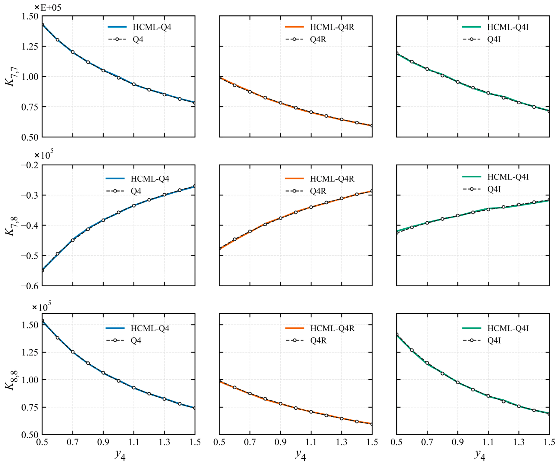
To further examine the predictive capability of the proposed model under continuous variations in element geometry, a regular unit-square element is taken as the baseline configuration. Only the vertical coordinate of node 4, , is varied continuously within the range of 0.50-1.50. For the three types of plane-stress elements, the selected independent stiffness entries are computed using both the trained neural-networks and reference elements. Their variations with respect to are then compared. The results show that the neural-network predictions almost overlap with the results of reference elements over the entire examined range, indicating that the proposed model can accurately capture the nonlinear variation of stiffness components induced by geometric distortion for different element types.
Figure 8.
Comparison of the neural-network predictions and results of reference elements for the stiffness components of Q4, Q4R, and Q4I elements as aries.
Figure 8.
Comparison of the neural-network predictions and results of reference elements for the stiffness components of Q4, Q4R, and Q4I elements as aries.
5. Implementation of the Direct Data-Driven Elements and Complete Flowchart
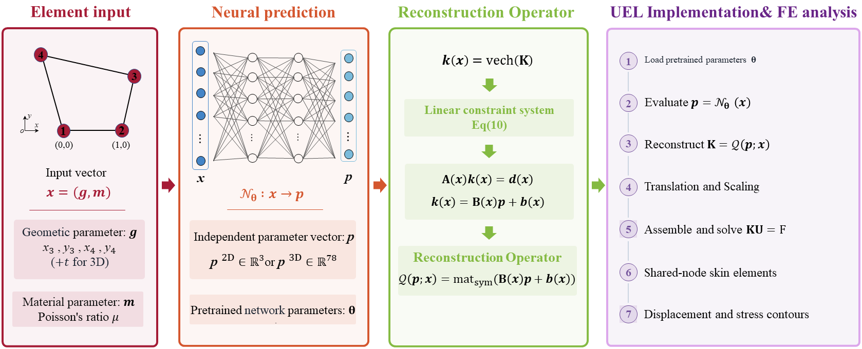
Figure 9 presents the complete computational workflow of the HCML-based direct data-driven elements, covering element input, neural-network prediction, element stiffness matrix reconstruction, and UEL-based finite element analysis. The element geometry and material parameters are first assembled into the input vector , from which the pretrained neural-network predicts the independent stiffness parameter vector . The full element stiffness matrix is then reconstructed from using the reconstruction operator derived from the linear system of physics-informed hard constraints. The learned elements are implemented through the Abaqus user element (UEL) interface, which enables user-defined element formulations to provide the element stiffness matrix and residual vector to the finite element solver through a Fortran subroutine. Before the finite element analysis, the parameters of the pretrained neural network are fixed and embedded into the UEL subroutine. During each UEL call, the subroutine successively performs element-input evaluation, neural-network forward propagation, hard-constrained stiffness-matrix reconstruction, stiffness scaling, and local-to-global coordinate transformation. The resulting element stiffness matrix and residual vector are returned to Abaqus for global assembly and equilibrium solution under the prescribed loads and boundary conditions. Finally, auxiliary skin elements, which share nodes with the UEL mesh and serve only as post-processing carriers without contributing to the structural stiffness, are employed when required to visualize the resulting displacement and stress fields.
6. Numerical Examples
This section presents numerical examples to test the performance of the HCML-FEs. All the learned element types have been summarized in Table 1. Section 6.1 presents fundamental numerical tests, including the rigid-body zero-energy mode test and the first-order patch tests for both plane-stress and solid-shell elements. Section 6.2 evaluates the performance of the HCML-Q4, HCML-Q4R, and HCML-Q4I elements with respect to mesh-distortion and mesh-dependence tests, as well as representative two-dimensional structural benchmarks, including Cook's skew beam and the strap plate problem. Section 6.3 assesses the HCML-SS8 element using three-dimensional solid-shell benchmarks, namely the Barrel vault roof problem, the Raasch Challenge problem, the hyperboloid-shell, and the thin-walled pipe elbow. Unless otherwise specified, all numerical examples in this section are performed using a consistent unit system.
6.1. Fundamental Numerical Tests
6.1.1. Rigid-Body Zero-Energy Mode Test
The rigid-body zero-energy mode test is a standard element-level verification of the null-space property of an element stiffness matrix.
For the two-dimensional elements, HCML-Q4, HCML-Q4R, and HCML-Q4I are tested using three quadrilateral geometries, namely a rectangular quadrilateral, an arbitrary quadrilateral, and a distorted quadrilateral, as shown in Figure 10(a)-11(c). For the three-dimensional case, HCML-SS8 is tested using a representative solid-shell geometry as shown in Figure 10(d).
For the HCML-FEs, Young's modulus and Poisson's ratio are set to 2E+04 and 0.3, respectively. For each test case, the complete element stiffness matrix is generated using the proposed physics-informed hard-constrained data-driven finite element formulation. The eigenvalues of the stiffness matrix are then computed and sorted in ascending order, and the number of near-zero eigenvalues is compared with the theoretical number of rigid-body modes, as shown in Table 3. In addition, the near-zero eigenvalue with maximum absolute value and the first nonzero eigenvalue are also included in Table 3.
From the results, the number of detected near-zero eigenvalues is consistent with the theoretical number of rigid-body modes for all tested elements and geometric configurations. The HCML-Q4, HCML-Q4R, and HCML-Q4I elements exhibit three near-zero eigenvalues under the rectangular, arbitrary quadrilateral, and distorted quadrilateral configurations, corresponding to two rigid-body translational modes and one out-of-plane rigid-body rotational mode. In contrast, the HCML-SS8 element exhibits six near-zero eigenvalues, corresponding to the six rigid-body modes in three-dimensional space. For all test cases, the near-zero eigenvalues are several orders of magnitude smaller than the first nonzero eigenvalue, indicating a clear separation between rigid-body modes and deformational modes. These near-zero eigenvalues can be attributed to numerical round-off errors, and no additional spurious zero-energy modes are observed. These results demonstrate that the proposed HCML-FEs successfully pass the rigid-body zero-energy mode test.
As shown in the last row of the table, the soft constraints method may yield a relatively small element stiffness matrix prediction error. However, the predicted element stiffness matrix does not retain the zero eigenvalues associated with rigid-body motions and therefore fails the rigid-body zero-energy mode test. The soft-constraint baseline illustrates a central distinction between stiffness-matrix prediction accuracy and finite-element admissibility. Although the predicted stiffness entries may remain close to the reference values, the rigid-body null space is not preserved. Thus, small regression errors alone are insufficient to define a mechanically valid element, whereas the HCML reconstruction preserves the prescribed null-space constraint by construction. Similarly, a finite element constructed from a soft-constraint baseline cannot precisely pass the patch test discussed in the next subsection.
6.1.2. Patch Test Under Constant Strain and Constant Generalized-Strain
The plane-stress patch test is first performed using arbitrary quadrilateral elements to evaluate the HCML-Q4, HCML-Q4R, and HCML-Q4I. The MacNeal-Harder patch geometry (MacNeal and Harder, 1985) is adopted, as shown in Figure 11. The boundary nodes are prescribed according to a linear displacement field, while the interior nodal displacements are obtained from the finite element solution. Young's modulus and Poisson's ratio are set to 2E+04 and 0.3. For the arbitrary quadrilateral patch, the displacement components in the x- and y-directions are prescribed at the boundary nodes as:
The analytical displacements prescribed by the linear displacement field and displacements computed with the HCML-FEs at the interior nodes are listed in Table 4. The displacement components are scaled by E-04.
The results show that the computed interior nodal displacements agree well with the analytical values, with relative differences on the order of E-08. This confirms that the arbitrary quadrilateral HCML-FE patch can reproduce the prescribed linear displacement field. Therefore, the arbitrary quadrilateral HCML-FEs pass the first-order plane-stress patch test.
The Constant generalized-strain patch test is then conducted for the three-dimensional HCML-SS8 element. As shown in Figure 12, a rectangular plate with uniform thickness is used as the test patch that is discretized by nine solid-shell elements with arbitrary quadrilateral midsurfaces. Young's modulus and Poisson's ratio are set to 2E+04 and 0.3. The external nodes are prescribed by a displacement field that produces a constant generalized-strain state, while the interior nodal displacements are solved from the finite element equilibrium equations with the proposed HCML-SS8. The imposed displacement field is given by:
The analytical displacements prescribed by Eq. (54) and the calculated displacements by the proposed HCML-SS8 at the interior nodes are summarized in Table 5. The displacement components are scaled by E-06.
The calculated displacements of the interior nodes are in excellent agreement with the analytical values. This result shows that the HCML-SS8 element can successfully pass the constant generalized-strain patch test and reproduce the constant bending/torsion response required for solid-shell deformation.
6.2. Structural Numerical Examples Using the HCML-Q4, HCML-Q4R and HCML-Q4I Elements
6.2.1. Mesh-Distortion and Mesh-Dependence Tests
MacNeal's cantilever beam benchmark (MacNeal and Harder, 1985) is used to evaluate mesh-distortion sensitivity and the performance of HCML-FEs with arbitrary quadrilateral elements. As shown in Figure 13, the length, height, and thickness of the beam are , and , respectively. Young's modulus and Poisson's ratio are set to 2E+04 and 0.3. The left end is clamped, and two loading cases are applied at the free end: (I) a tip shear force of and (II) a tip bending moment of . Three mesh patterns are examined: a regular mesh, a parallelogram mesh, and a trapezoidal mesh, denoted as Mesh I, Mesh II, and Mesh III, respectively. In this benchmark, we mainly compare the vertical displacement at point A for two load cases and three mesh patterns. Here, the reference vertical displacements are for load and for load. All the HCML-Q4, HCML-Q4R, and HCML-Q4I elements are examined and compared with their corresponding reference elements, respectively, as shown in Table 6.
Table 6 summarizes the vertical displacement obtained by reference elements and the HCML-FEs under different mesh levels. The reported displacement values are scaled by E-02. The benchmark is bending-dominated, and only one element is used through the thickness direction; therefore, it is sensitive to both the element formulation and mesh distortion. Except for Q4R and HCML-Q4R, the computational results of the HCML-FEs for the other two element types are close to those of the corresponding reference elements.
The results show that the present benchmark employs arbitrary quadrilateral meshes, and mesh distortion has a pronounced influence on the numerical response of low-order quadrilateral elements. Except for Q4R and HCML-Q4R, the HCML-FEs show good agreement with the corresponding reference elements and are able to reproduce the mesh-dependence characteristics of different reference formulations. Both Q4 and HCML-Q4 exhibit an overly stiff response, and mesh distortion further reduces the displacement magnitude. Q4I and HCML-Q4I provide relatively high accuracy on the regular mesh, but over-stiffening is still observed under distorted meshes, indicating that the incompatible-mode formulation improves bending performance but its effectiveness is sensitive to mesh distortion, which is like the nonconforming elements. In contrast, Q4R and HCML-Q4R exhibit evident hourglass-dominated responses in coarse distorted-mesh cases. The Q4R results also clarify the role of the training data in the proposed framework. The hard constraints define the mechanically admissible structure imposed on the learned stiffness matrix, but they do not remove numerical characteristics from the reference data that are not excluded by these constraints. Consequently, undesirable behavior contained in the reference element, such as the pronounced coarse-mesh sensitivity of the reduced-integration formulation, may also be inherited. In this sense, the physical constraints determine admissibility, whereas the reference data determine the remaining numerical character of the learned element.
6.2.2. Cook's Skew Beam
Cook et al.’s (2001) skew beam benchmark is used to evaluate the performance under combined geometric distortion and mesh refinement of the proposed HCML-FEs, as shown in Figure 14. Young's modulus and Poisson's ratio are set to 2E+04 and 0.3. The left edge is fully clamped, and a vertical upward concentrated load is applied at point A on the right end. The geometric inclination angle is denoted by . When , the vertical displacement at point A is considered, and its theoretical value is = 1.20E-04. For the Cook’s skew beam benchmark, the same number of mesh seeds, denoted by , is assigned along each of the four edges. The domain is then discretized into arbitrary quadrilateral elements. It is evident that different values of the inclination angle lead to different levels of element and mesh distortion.
When , Table 7 summarizes the maximum vertical displacement obtained by reference elements and the HCML-Fes under different mesh levels. The reported displacement values are scaled by E-04. Figure 15 shows the displacement and von Mises stress contours of Q4I and HCML-Q4I for . The results show that, in the Cook’s skew beam problem, the HCML-FEs can reproduce the typical convergence behavior of the corresponding reference elements. The Q4 and HCML-Q4 elements underestimate the displacement on coarse meshes, reflecting the relatively stiff response of bilinear quadrilateral elements in bending-dominated skew geometries. The Q4R and HCML-Q4R elements exhibit stronger coarse-mesh sensitivity, but their responses gradually stabilize with mesh refinement. In contrast, owing to their improved bending representation, the Q4I and HCML-Q4I elements remain closer to the benchmark reference solution over a wider range of mesh densities. Meanwhile, the displacement and von Mises stress contours of Q4I and HCML-Q4I shown in Figure 15 for exhibit generally consistent field distributions.
To further demonstrate the generalization capability of the HCML framework, Figure 16 compares the vertical displacement at point A and its relative error between Q4I and HCML-Q4I under different geometric inclination angles. Figure 16 shows that, as the geometric inclination angle increases, some element interior angles gradually fall outside the coverage of the training dataset, with the minimum interior angle becoming smaller than . For moderately out-of-domain geometries, the proposed HCML-Q4I still maintains acceptable prediction accuracy. However, the displacement error increases markedly as further increases, indicating that the learned element possesses a certain degree of geometric generalization and extrapolation capability, although this capability is limited to a finite range of geometric distortion. By expanding the training domain, specifically by reducing the lower bound of the minimum interior angle to , the relative errors between HCML-Q4I and Q4I are kept within approximately 1.1%, even when deviates from . Overall, the HCML-FEs not only accurately reproduce the responses of the corresponding reference elements and exhibit a reasonable convergence trend toward the benchmark reference solution, but also demonstrate a certain degree of geometric generalization and extrapolation capability. The results distinguish two forms of generalization. Within the sampled geometric domain, the learned element reproduces the reference response over continuously varying element shapes. Outside this domain, the mechanical constraints remain exactly satisfied, whereas the accuracy of the unconstrained stiffness information gradually deteriorates as the geometry moves farther from the training range.
6.2.3. Strap Plate Problem
The strap plate benchmark is used to assess the applicability of the proposed HCML-FEs to perforated structures with practical geometric complexity and pronounced local stress concentrations. As shown in Figure 17, the plate contains three circular holes. All nodes on the boundaries of the two left holes are fully constrained, and a concentrated load is applied at point A, located at the top of the right hole, in the negative y-direction. Three mesh densities labeled as Mesh I, Mesh II, and Mesh III in Figure 17 are adopted to examine the mesh-dependence behavior of the numerical response. The considerable variations in element shape and size within this mesh provide a stringent test of the geometric generalization capability of the HCML-FEs. Young's modulus and Poisson's ratio are set to 2E+04 and 0.3. The reference value of the vertical nodal displacement at the loaded point A is -5.374 E-04, which is obtained using a highly refined mesh.
Table 8 compares the maximum vertical nodal displacement at the loaded point A obtained by reference elements and the HCML-FEs under different mesh densities. The reported displacement values are scaled by E-04. Figure 18 presents the displacement and von Mises stress contours of Q4I and HCML-Q4I for Mesh I. The results show that, under different mesh densities, the learned elements remain in good agreement with their corresponding reference elements and exhibit consistent convergence trends. Figure 18 further indicates that HCML-Q4I and Q4I show highly consistent full-field displacement distributions, von Mises stress distributions, and stress-concentration regions near the loaded area. Overall, the strap plate benchmark demonstrates that the proposed HCML-FEs can be applied to engineering structures with complex geometric features and can accurately reproduce the mechanical responses of the corresponding reference elements.
6.3. Complex Numerical Examples for the HCML-SS8 Element
6.3.1. Barrel Vault Roof
The Barrel vault roof benchmark is used to evaluate the performance of the proposed learned solid-shell element in a cylindrical shell problem involving coupled membrane and bending deformation. As shown in Figure 19, the roof has a length , radius , and thickness . Young's modulus and Poisson's ratio are set to 2E+11 and 0.3. The four boundary edges are fully clamped, and uniformly distributed loading is represented by equivalent nodal forces applied in the global z-direction. The model is discretized using 25×16×1 and 50×32×2 meshes, where the three values denote the numbers of elements in the longitudinal, circumferential, and thickness directions, respectively. For the initial 25×16×1 mesh, a unit vertical nodal load is applied to each node in the z-direction. After mesh refinement, the nodal force is adjusted according to the number of loaded nodes so that the total applied load remains unchanged.
Table 9 presents the relative errors in the maximum z-direction displacement between HCML-SS8 and SS8 for the two meshes. The displacement values are scaled by E-10. Figure 20 and Figure 21 compare the z-direction displacement and von Mises stress contours obtained using SS8 and HCML-SS8 on the 25×16×1 mesh.
The results demonstrate that the HCML-SS8 solution approaches the SS8 reference solution as the mesh is refined. The two elements exhibit consistent overall deformation modes, displacement gradients, and locations of the maximum-displacement region. The von Mises stress distributions on the top surface, midsurface, and bottom surface also show good agreement in their spatial patterns and principal stress-concentration regions. Together with the reduction in the displacement difference after mesh refinement, these results indicate that HCML-SS8 reproduces the dominant membrane–bending coupled response of the reference SS8 element within the investigated meshes.
6.3.2. Raasch Challenge
The Raasch Challenge is a classical shell benchmark commonly used to assess the capability of shell elements in representing coupled shear, bending, and twisting deformation in curved thin-strip structures. As shown in Figure 22, one end of the structure is rigidly clamped, while a nodal load with a magnitude of 1 is applied to each node at the free end in the positive z-direction. The material is assumed to be linearly elastic. Young's modulus and Poisson's ratio are set to 2E+11 and 0.3, respectively. The model is discretized using a structured SS8 mesh of 20×144×2, where 20, 144, and 2 denote the numbers of elements along the width, curved longitudinal, and thickness directions, respectively.
Figure 23 compares the z-direction displacement contours and the bottom-surface von Mises stress contours obtained using the SS8 element and the HCML-SS8 element. The reported displacement values are scaled by E-06. The two elements exhibit good agreement in terms of the overall deformation pattern, displacement distribution, and stress-field distribution. The relative error in the maximum nodal displacement in the z-direction is 2.83%, indicating that HCML-SS8 can accurately reproduce the displacement response of SS8.
Because the Raasch Challenge involves strongly coupled in-plane bending, transverse shear, and twisting deformations, this agreement demonstrates that HCML-SS8 effectively reproduces the capability of SS8 to represent the complex coupled response under the discretization conditions considered. Furthermore, the displacement and stress fields vary smoothly across the junction of the two circular segments, without evident local numerical oscillations, nonphysical discontinuities, or spurious flexibility. Overall, this benchmark confirms the applicability and reliability of HCML-SS8 for curved shell structures involving coupled deformation modes.
6.3.3. Hyperboloid-Shell
The model is a sector of a shell of revolution generated by rotating an offset semi-elliptical meridian about the y-axis. As shown in Figure 24, the shell has a waist diameter , an end diameter , and an axial length , and a uniform thickness . The two longitudinal cut edges lying in the plane are fully clamped. A concentrated nodal force of 1E+04 is applied in the negative global z-direction at the node A located at the center of the inner surface. Young's modulus and Poisson's ratio are set to 2E+11 and 0.3, respectively. The model is discretized using coarse and refined structured meshes of 70×54×1 and 140×108×2, respectively, where the three numbers denote the numbers of elements in the circumferential, axial, and through-thickness directions. Thus, the refined mesh doubles the number of elements in each of the three directions relative to the coarse mesh.
Table 10 summarizes the maximum z-direction displacement at the loaded point A obtained by SS8 and HCML-SS8 with the coarse and refined meshes, together with the corresponding relative differences. Figure 25 compares the z-direction displacement contours and the bottom-surface von Mises stress contours obtained using the coarse 70×54×1 mesh. The reported displacement and stress values are scaled by E-06 and E+03, respectively.
To quantify the geometric deviation of the actual three-dimensional elements from the training samples, the angle between each thickness edge and the corresponding fitted midsurface normal is adopted as an indicator of thickness-direction distortion. For the ideal solid-shell training samples generated by normal extrusion of the midsurface, this deviation angle is . A larger deviation angle indicates a more pronounced departure from the canonical normal-extrusion configuration. The thickness-edge deviation angles for the three solid-shell benchmark cases are summarized in Table 11.
Compared with the benchmarks in Section 6.3.1 and Section 6.3.2, the present problem is more challenging because the shell involves opposite curvatures along two orthogonal directions. As a result, the generated solid-shell elements are not uniformly aligned through the thickness and deviate more significantly from the canonical midsurface-extrusion configurations used in the training stage, as shown in Table 11. Nevertheless, the numerical results show that HCML-SS8 remains stable for this more complex geometry. Moreover, the relative difference between the displacements predicted by SS8 and HCML-SS8 decreases further as the mesh is refined from 70×54×1 to 140×108×2. Both the displacement and stress fields preserve the main deformation characteristics of the SS8 reference solution. These results further indicate that the HCML-SS8 retains a certain degree of robustness and limited out-of-distribution generalization capability under geometric conditions that are more complex than the training configurations.
6.3.4. Thin-Walled Pipe Elbow
To assess the applicability of the proposed element in mixed-element analysis, a thin-walled pipe elbow with two straight end sections is considered, as shown in Figure 26. This mixed-element example verifies a defining requirement of numerical-method construction emphasized in Section 1: the learned element can participate in the same global assembly process as conventional finite elements and is not tied to an isolated learned computational domain. The elbow has a centerline radius of , inner and outer pipe radii of 20 and 21, respectively, and a corresponding wall thickness of . Each straight end section has a length of 50. One end of the pipe is fully clamped, while a concentrated nodal force of is applied to each node on the annular cross-section at the other end. The two straight pipe sections are discretized using solid-shell elements, with 25×56×2 elements in each section, whereas the elbow is discretized using 33×56×2 Q8R elements. Young's modulus and Poisson's ratio are set to 2E+11 and 0.3.
Figure 27 compares the maximum nodal displacements in the z-direction and the top-surface von Mises stress contours obtained from the two mixed-element models. The reported displacement and stress values are scaled by E-05 and E+04, respectively. In both models, the elbow is discretized using Q8R elements, whereas the two straight pipe sections are modeled using either SS8 or HCML-SS8 elements. The maximum z-direction nodal displacement obtained from the HCML-SS8 and Q8R model differs from that predicted by the SS8 and Q8R model by only 0.24%, indicating close agreement in the predicted global structural flexibility. The two models also produce generally consistent principal stress-concentration regions, spatial distribution patterns, and stress-variation trends, with no evident local stress oscillations or nonphysical stress concentrations near the HCML-SS8 and Q8R interfaces.
7. Discussion and Conclusions
7.1. Discussion
The present results highlight a distinction between stiffness-matrix prediction and finite-element construction. A small regression error does not necessarily lead to a mechanically admissible element, as illustrated by the soft-constraint baseline. For data-driven numerical-method construction, the learned operator must therefore satisfy the structural requirements of the numerical method itself, rather than only approximate reference outputs. In the HCML framework, this is achieved by embedding the physical-informed hard constraints into the stiffness reconstruction through Symbolic derivation.
The results also clarify the different roles of physical(mechanics) and data. The hard constraints determine the admissible structure of the learned stiffness matrix, whereas the reference data determine the remaining element-specific numerical characteristics. This explains why elements learned from Q4, Q4R, Q4I and SS8 retain different numerical behaviors even though they are constructed through the same HCML procedure. The framework should therefore not be interpreted as an automatic improvement of the reference formulation. In this sense, mechanics defines what the learned element must satisfy, while data determine which element is constructed within those requirements.
The use of existing finite-element formulations as reference-data sources should be understood as a controlled setting for examining this construction problem. Their numerical characteristics are known in advance, making it possible to assess whether the HCML framework can reproduce element-level behavior while preserving the prescribed mechanical constraints and the locality, reusability, and assemblability required for finite-element analysis. Importantly, HCML does not rely on the variational formulation, interpolation functions, quadrature rules, stabilization procedures, or other internal details of the reference data; it requires only suitable element-level stiffness information. The origin of that information is therefore conceptually separate from the HCML construction itself.
7.2. Conclusion and Outlook
This work investigated whether data-driven learning can be used to construct a reusable numerical method rather than only approximate the solution of a prescribed boundary-value problem. Using finite elements as a representative setting, we developed a physics-informed Hard-Constrained Manifold Learning (HCML) framework. Under the prescribed linear constraints, symbolic elimination reduces the stiffness description to three independent parameters for the four-node plane-stress element and 78 for the eight-node solid-shell element. A neural network predicts only these independent quantities, while the complete stiffness matrix is recovered through a deterministic reconstruction operator. Numerical tests further show that the resulting HCML-FEs retain the characteristic responses of different reference formulations under bending, locking, mesh distortion, and mesh refinement, while remaining reusable and assemblable in different two- and three-dimensional structural problems.
The present work focuses on the construction problem once suitable element-level reference stiffness information is available. Further development may investigate how such information can be obtained independently of existing finite-element formulations. In particular, deriving discrete element information directly from continuum-mechanics analytical solutions, experimental observations, or other physically consistent sources requires an additional continuum-to-discrete construction procedure and constitutes a separate problem from the HCML formulation considered here. Extensions to nonlinear material behavior, finite deformation, and additional element families also remain to be investigated.
Data Availability Statement
Data will be made available on request.
Acknowledgments
This work was supported by the National Natural Science Foundation of China (Grant Nos. 12572123) and the Liaoning Provincial Natural Science Foundation (Grant No. 2025-MS-011).
CRediT Authorship Contribution Statement: Shuyuan Li: Writing – review & editing, Writing – original draft, Software, Methodology, Investigation, Formal analysis, Conceptualization; Yuan Liang: Writing – review & editing, Methodology, Investigation, Formal analysis, Conceptualization.
Declaration of Competing Interests: The authors declare that they have no known competing financial interests or personal relationships that could have appeared to influence the work reported in this paper.
Appendix A. Constraint Derivation for the Normalized Plane-Stress Quadrilateral Element
A.1 Geometric Configuration and Degrees of Freedom
The normalized geometry of the quadrilateral element is shown in Figure 2, and its geometric input parameters are defined in Eq. (26). The material is assumed to be linear elastic and isotropic under plane-stress conditions, with unit thickness; the corresponding element stiffness matrix is denoted by . For clarity in the subsequent derivation, the nodal degree-of-freedom ordering in Eq. (25) is not adopted in this appendix. Instead, the following ordering is used throughout:
The degree-of-freedom ordering in Eq. (A.1) is used consistently for the stiffness matrix, displacement modes, nodal force vector, and the symbolic computation program in Appendix B.
A.2 Rigid-Body Zero-Energy Constraints
Taking rigid translations along the global x- and y-directions and an in-plane rigid rotation about the coordinate origin as the three displacement modes gives the rigid-body mode matrix :
Rigid-body motion produces neither strain energy nor internal nodal forces; therefore,
A.3 Constant-Strain Consistency Constraint
For the displacement field assumed in Eq. (28), the three columns of reproduce a unit normal strain in the x-direction, ; a unit normal strain in the y-direction, ; and a unit engineering shear strain, , respectively. The shear mode is represented by a symmetric displacement field.
This modal representation corresponds to the constant-strain vector defined in Eq. (29).
Under plane-stress conditions, the element stress can be expressed as
where is Young's modulus and is Poisson's ratio.
A.4 Boundary Tractions and Consistent Equivalent Nodal Forces
Let edge connect node to node . Cyclic numbering is adopted, such that node 5 is identical to node 1. The coordinate increments, edge length, and outward unit normal are defined as follows:
The traction vector on each element edge follows from Cauchy's traction formula:
The outward unit normal associated with edge 1 in Figure 2 is
Accordingly, the traction vector on edge 1 is given by
Following the consistent nodal-force equivalence principle, the continuous traction on edge 1 is integrated along the boundary using the linear shape functions and distributed equivalently to the two end nodes. The consistent equivalent nodal forces at nodes 1 and 2 are therefore
The equivalent nodal forces associated with the remaining three edges are obtained in the same manner. Summing the contributions from all four edges according to the prescribed degree-of-freedom ordering gives the following unified expression for the nodal force vector :
The nodal force column vectors corresponding to the unit normal strains and , and the unit shear strain , can therefore be extracted and assembled into the consistent equivalent nodal force matrix associated with the three constant-strain modes.
The constant-strain consistency constraint can thus be written as
Appendix B. Reproducible Symbolic Gaussian Elimination and Identification of Independent Stiffness Parameters
This appendix supplements Section 3.1.3 by providing a Python program that identifies the locations of the three independent stiffness parameters for the two-dimensional plane-stress quadrilateral element. It also outputs the complete symbolic reconstruction relations between the independent and dependent stiffness entries. The code can be readily extended to handle the subsequent three-dimensional case.

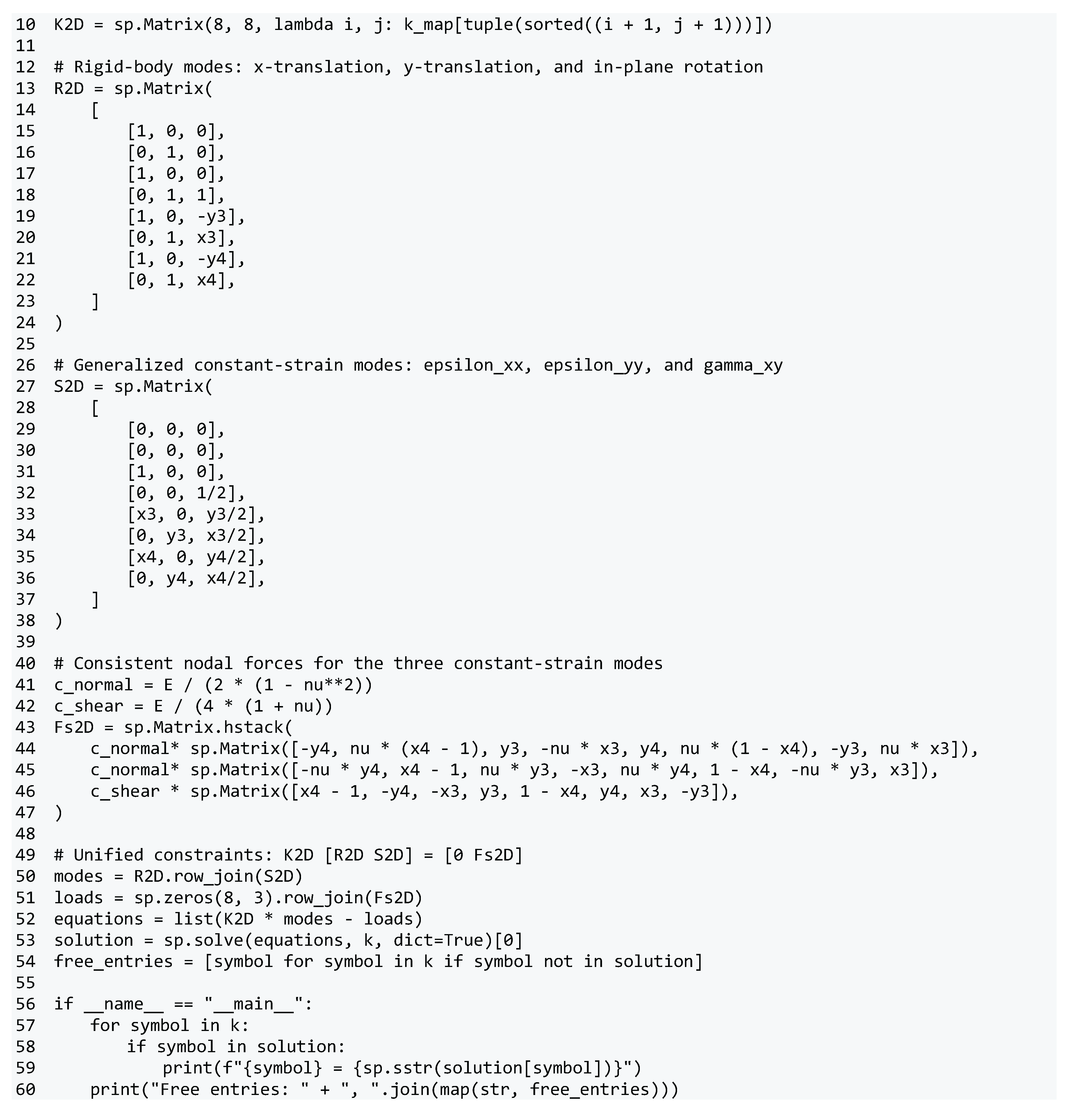
Appendix C. Training Settings and Convergence Curves
A multilayer perceptron is adopted to approximate the nonlinear mapping from the element input vector to the independent stiffness parameter vector. For a general input vector , the computation of the -th hidden layer is written as
where and denote the weight matrix and bias vector of the -th layer, respectively, and is the activation function. The network output is the predicted independent stiffness parameter vector . Mish is employed as the activation function for all hidden layers due to its smooth nonlinearity and stable convergence behavior observed in the present experiments. For each element type, the training dataset is divided into training, validation, and test subsets with a ratio of 6:3:1, which are used for model fitting, hyperparameter selection, and final generalization assessment, respectively. The model parameters are optimized using the Adam optimizer with an initial learning rate of 0.01.A multi-step learning-rate scheduler is used, in which the learning rate is multiplied by 0.1 at epochs 4000, 8000, 12000, and 16000. Full-batch training is adopted, meaning that each epoch performs one parameter update using the entire training set. All models are trained for 18000 epochs. No explicit weight decay is used in the reported baseline models, and overfitting is monitored through the validation loss.
To evaluate the training stability of the proposed physics-informed hard-constrained manifold learning framework, the convergence histories of the training and validation losses are examined separately for the four-node plane-stress quadrilateral elements and the eight-node solid-shell element. Consistent with the training strategy described in Section 4.2, the reported loss is the mean-squared error evaluated in the independent stiffness parameter space.
The training and validation loss curves for HCML-Q4, HCML-Q4I, HCML-Q4R, and HCML-SS8 are shown in Figure 28(a)-(d), respectively. All four elements exhibit similar convergence behavior: the training and validation losses decrease rapidly during the early stage, show moderate fluctuations before the first learning-rate reduction, and subsequently become smoother and gradually converge. After approximately 4000 epochs, both losses decrease slowly toward stable levels. The final losses of Q4, Q4I, and Q4R are on the order of E-04, whereas SS8 converges to a relatively higher loss level because of its higher-dimensional independent stiffness parameter vector and more complex stiffness response.
Figure 28.
Training and validation loss curves for different element types: (a) HCML-Q4; (b) HCML-Q4I; (c) HCML-Q4R; (d) HCML-SS8.
Figure 28.
Training and validation loss curves for different element types: (a) HCML-Q4; (b) HCML-Q4I; (c) HCML-Q4R; (d) HCML-SS8.
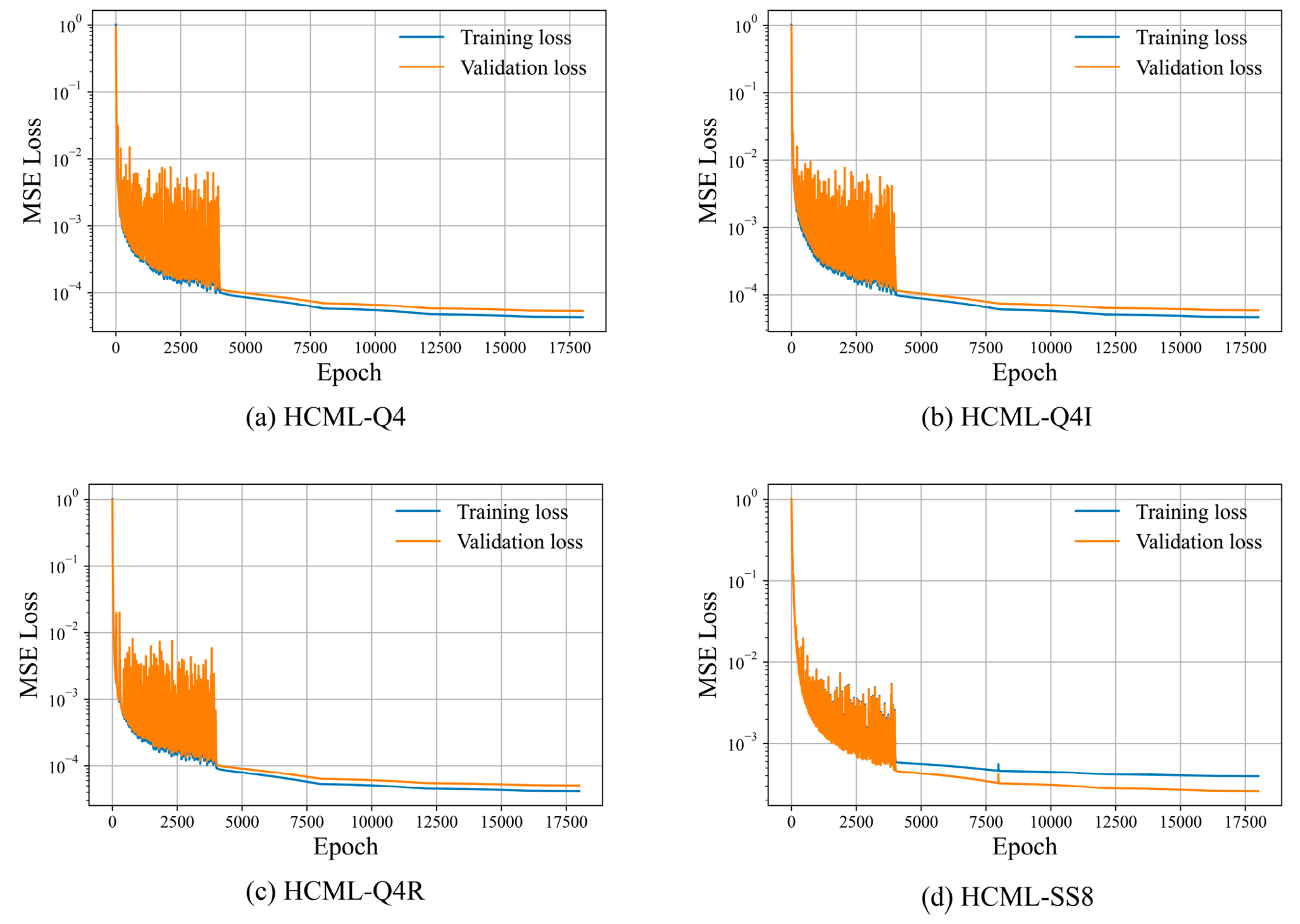
For all four elements, the validation losses remain close to the corresponding training losses after convergence and exhibit no continuously increasing trend. Although no explicit regularization or weight-decay penalty is included in the loss function, no evident overfitting is observed. These results demonstrate that the proposed network can stably learn the independent stiffness parameter vectors of different element types while maintaining satisfactory generalization performance on the validation datasets.
References
- Abed-Meraim, F.; Combescure, A. SHB8PS: a new adaptive, assumed-strain continuum mechanics shell element for impact analysis. Comput. Struct. 2002, 80, 791–803. [Google Scholar] [CrossRef]
- Bathe, K.J. Finite Element Procedures, second ed.; K.J. Bathe: Watertown, MA, 2014. [Google Scholar]
- Bathe, K.J.; Dvorkin, E.N. A formulation of general shell elements—the use of mixed interpolation of tensorial components. Int. J. Numer. Methods Eng. 1986, 22, 697–722. [Google Scholar] [CrossRef]
- Cook, R.D.; Malkus, D.S.; Plesha, M.E.; Witt, R.J. Concepts and Applications of Finite Element Analysis, fourth ed.; Wiley: New York, 2001. [Google Scholar]
- Dong, Y.; Liu, T.; Li, Z.; Qiao, P. DeepFEM: a novel element-based deep learning approach for solving nonlinear partial differential equations in computational solid mechanics. J. Eng. Mech. 2023, 149, 04022102. [Google Scholar] [CrossRef]
- Enabe, P.A.F.; Provasi, R. A hybrid virtual element method and deep learning approach for solving one-dimensional Euler–Bernoulli beams. Appl. Math. Comput. 2025, 507, 129600. [Google Scholar] [CrossRef]
- Haghighat, E.; Raissi, M.; Moure, A.; Gomez, H.; Juanes, R. A physics-informed deep learning framework for inversion and surrogate modeling in solid mechanics. Comput. Methods Appl. Mech. Eng. 2021, 379, 113741. [Google Scholar] [CrossRef]
- Hauptmann, R.; Schweizerhof, K. A systematic development of solid-shell element formulations for linear and nonlinear analyses employing only displacement degrees of freedom. Int. J. Numer. Methods Eng. 1998, 42, 49–69. [Google Scholar] [CrossRef]
- Hughes, T.J.R. The Finite Element Method: Linear Static and Dynamic Finite Element Analysis; Dover Publications: Mineola, NY, 2000. [Google Scholar]
- Jia, G.; Yu, Y.; Wang, D. Solving finite element stiffness matrix based on convolutional neural network. J. Beijing Univ. Aeronaut. Astronaut. 2020, 46, 481–487. [Google Scholar]
- Jung, J.; Jun, H.; Lee, P.S. Self-updated four-node finite element using deep learning. Comput. Mech. 2022, 69, 23–44. [Google Scholar] [CrossRef]
- Jung, J.; Yoon, K.; Lee, P.S. Deep learned finite elements. Comput. Methods Appl. Mech. Eng. 2020, 372, 113401. [Google Scholar] [CrossRef]
- Karniadakis, G.E.; Kevrekidis, I.G.; Lu, L.; Perdikaris, P.; Wang, S.; Yang, L. Physics-informed machine learning. Nat. Rev. Phys. 2021, 3, 422–440. [Google Scholar] [CrossRef]
- Kim, Y.Y.; Yu, M.; Yoon, K.; Noh, G. Learned Gaussian quadrature for continuum-mechanics-based beam finite elements. Comput. Methods Appl. Mech. Eng. 2026, 457, 118972. [Google Scholar] [CrossRef]
- Li, C.; Yang, S.; Zheng, H.; Zhang, Y.; Wu, L.; Xue, W.; Shen, D.; Lu, W.; Ni, Z.; Liu, M.; He, L. Integration of machine learning with finite element analysis in materials science: a review. J. Mater. Sci. 2025, 60, 8285–8307. [Google Scholar] [CrossRef]
- Liu, Y.; Park, C.; Lu, Y.; Mojumder, S.; Liu, W.K.; Qian, D. HiDeNN-FEM: a seamless machine learning approach to nonlinear finite element analysis. Comput. Mech. 2023, 72, 173–194. [Google Scholar] [CrossRef] [PubMed]
- Lu, L.; Meng, X.; Mao, Z.; Karniadakis, G.E. DeepXDE: a deep learning library for solving differential equations. SIAM Rev. 2021, 63, 208–228. [Google Scholar] [CrossRef]
- MacNeal, R.H.; Harder, R.L. A proposed standard set of problems to test finite element accuracy. Finite Elem. Anal. Des. 1985, 1, 3–20. [Google Scholar] [CrossRef]
- Nath, S.S.; Nath, D.; Gautam, S.S. Design of efficient finite elements using deep learning approach. In Advances in Engineering Design: Select Proceedings of FLAME 2022; Sharma, R., Kannojiya, R., Garg, N., Gautam, S.S., Eds.; Springer: Singapore, 2023; pp. 11–20. [Google Scholar]
- Ouyang, W.; Shin, Y.; Liu, S.W.; Lu, L. Neural-operator element method: efficient and scalable finite element method enabled by reusable neural operators. arXiv 2025, arXiv:2506.18427. [Google Scholar]
- Park, S.; Jung, J.; Lee, P.S. Towards improving the self-updated four-node finite element. Comput. Struct. 2026, 321, 108014. [Google Scholar] [CrossRef]
- Raissi, M.; Perdikaris, P.; Karniadakis, G.E. Physics-informed neural networks: a deep learning framework for solving forward and inverse problems involving nonlinear partial differential equations. J. Comput. Phys. 2019, 378, 686–707. [Google Scholar] [CrossRef]
- Reese, S. A large deformation solid-shell concept based on reduced integration with hourglass stabilization. Int. J. Numer. Methods Eng. 2007, 69, 1671–1716. [Google Scholar] [CrossRef]
- Simo, J.C.; Armero, F. Geometrically non-linear enhanced strain mixed methods and the method of incompatible modes. Int. J. Numer. Methods Eng. 1992, 33, 1413–1449. [Google Scholar] [CrossRef]
- Simo, J.C.; Rifai, M.S. A class of mixed assumed strain methods and the method of incompatible modes. Int. J. Numer. Methods Eng. 1990, 29, 1595–1638. [Google Scholar] [CrossRef]
- Stummel, F. The generalized patch test. SIAM J. Numer. Anal. 1979, 16, 449–471. [Google Scholar] [CrossRef]
- Subhash, T.V.K.; Ankit; Nath, D.; Gautam, S.S. Machine learning assisted development of eight-node hexahedral finite element. In Recent Advances in Aerospace Engineering: Select Proceedings of MRAE 2023; Singh, S., Ramulu, P.J., Gautam, S.S., Eds.; Springer: Singapore, 2024; pp. 241–251. [Google Scholar]
- Tandale, S.B.; Markert, B.; Stoffel, M. Smart stiffness computation of one-dimensional finite elements. Mech. Res. Commun. 2022, 119, 103817. [Google Scholar] [CrossRef]
- Valente, M.; Dias, T.C.; Guerra, V.; Ventura, R. Physics-consistent machine learning with output projection onto physical manifolds. Commun. Phys. 2025, 8, 433. [Google Scholar] [CrossRef]
- Xiong, W.; Long, X.; Bordas, S.P.A.; Jiang, C. The deep finite element method: a deep learning framework integrating the physics-informed neural networks with the finite element method. Comput. Methods Appl. Mech. Eng. 2025, 436, 117681. [Google Scholar] [CrossRef]
- Yu, M.; Kim, S.; Noh, G. Learned Gaussian quadrature for enriched solid finite elements. Comput. Methods Appl. Mech. Eng. 2023, 414, 116188. [Google Scholar] [CrossRef]
- Zienkiewicz, O.C.; Taylor, R.L.; Zhu, J.Z. The Finite Element Method: Its Basis and Fundamentals, seventh ed.; Butterworth-Heinemann: Oxford, 2013. [Google Scholar]
Figure 1.
Conceptual comparison between data-driven PDE solution and the proposed HCML-based data-driven numerical method construction.
Figure 1.
Conceptual comparison between data-driven PDE solution and the proposed HCML-based data-driven numerical method construction.
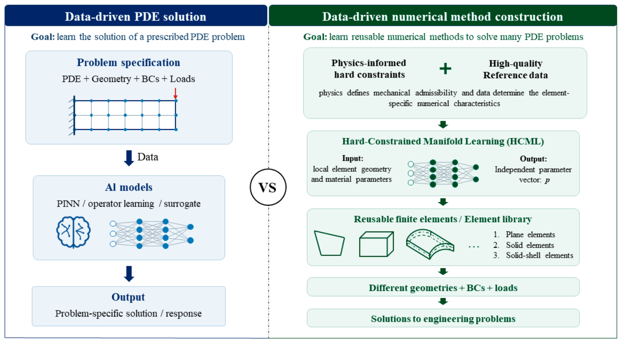
Figure 2.
Normalized geometry of the quadrilateral element.
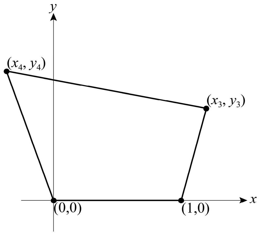
Figure 3.
Geometric normalization of an arbitrary quadrilateral element.
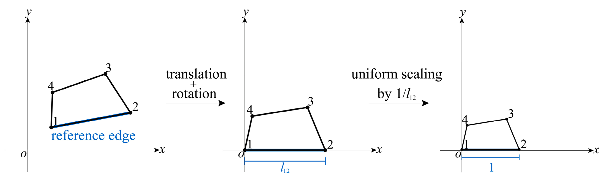
Figure 4.
Locations of independent and non-independent entries in the stiffness matrix of the quadrilateral element.
Figure 4.
Locations of independent and non-independent entries in the stiffness matrix of the quadrilateral element.
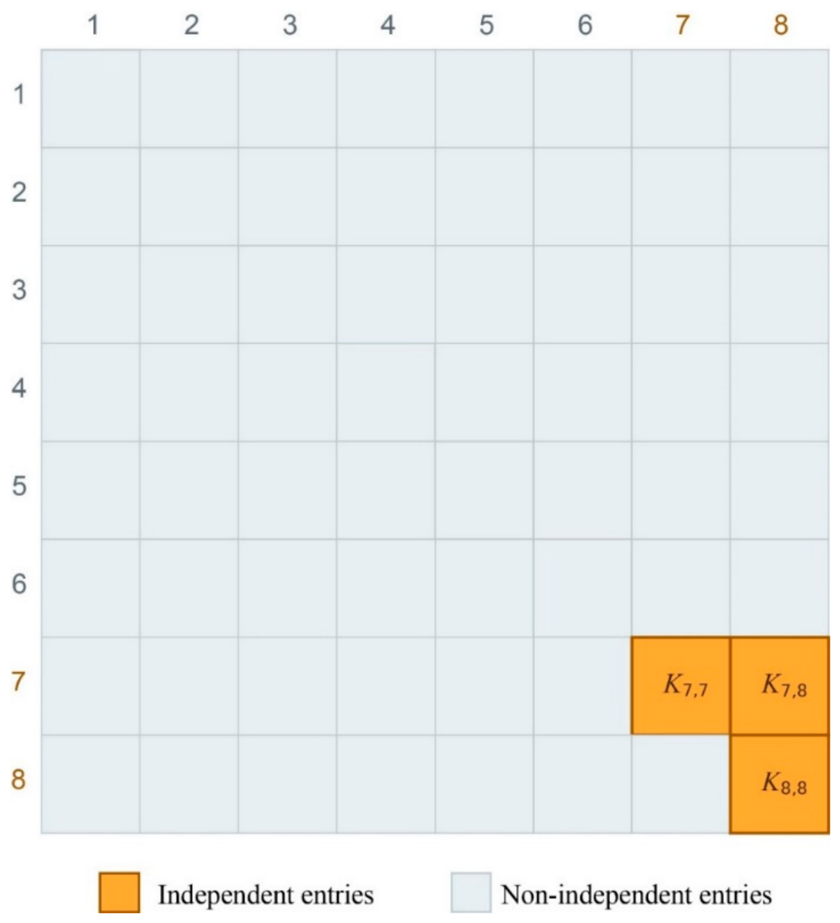
Figure 5.
Normalized geometry of the solid-shell element constructed by midsurface extrusion.
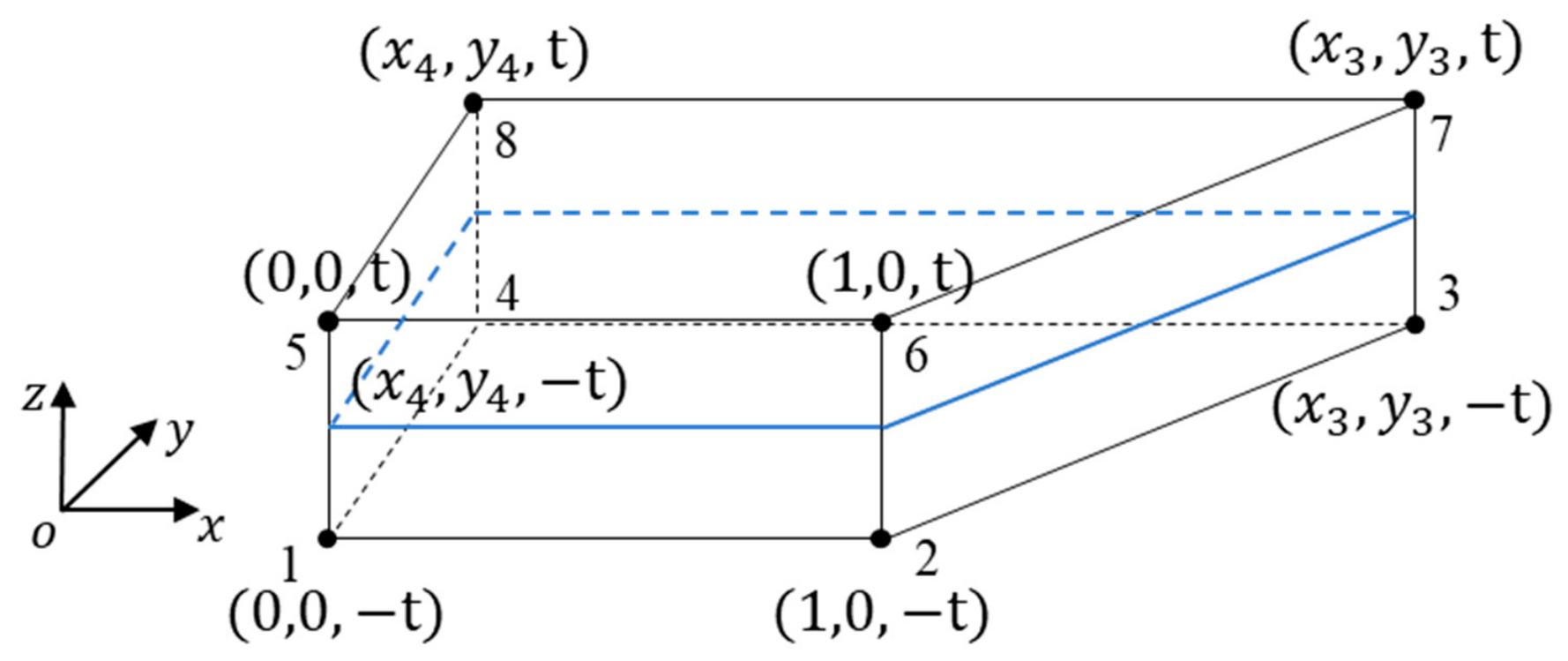
Figure 6.
Locations of independent and non-independent entries in the stiffness matrix of the solid-shell element.
Figure 6.
Locations of independent and non-independent entries in the stiffness matrix of the solid-shell element.
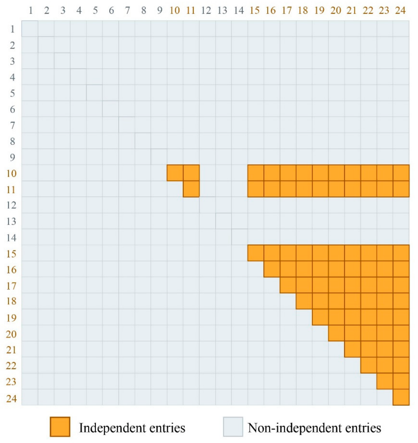
Figure 7.
Admissible sampling regions for the normalized quadrilateral element geometry.
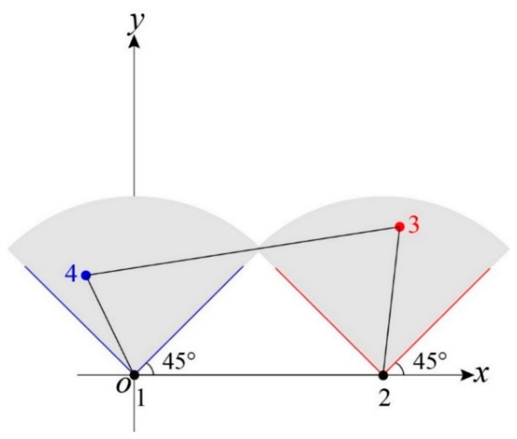
Figure 9.
Overall workflow of the HCML-based direct data-driven finite element framework and its UEL implementation.
Figure 9.
Overall workflow of the HCML-based direct data-driven finite element framework and its UEL implementation.
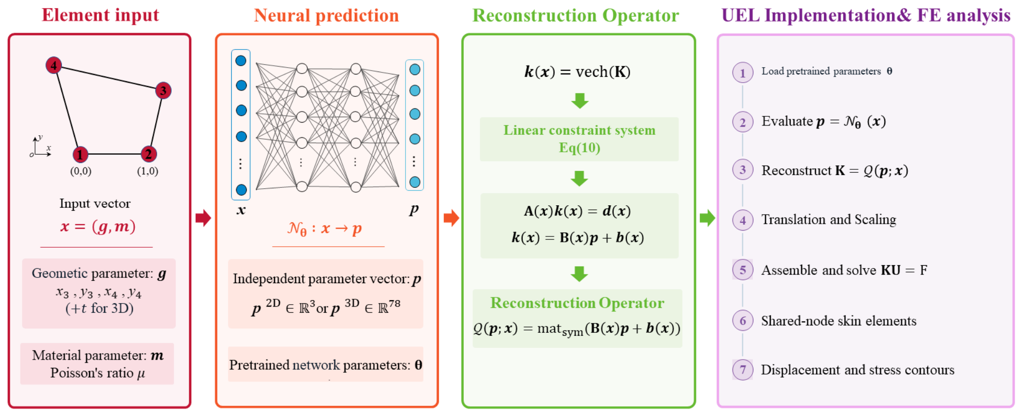
Figure 10.
Representative geometric configurations used in the rigid-body zero-energy mode test: (a) rectangular quadrilateral; (b) arbitrary quadrilateral; (c) distorted quadrilateral; (d) solid-shell geometry.
Figure 10.
Representative geometric configurations used in the rigid-body zero-energy mode test: (a) rectangular quadrilateral; (b) arbitrary quadrilateral; (c) distorted quadrilateral; (d) solid-shell geometry.
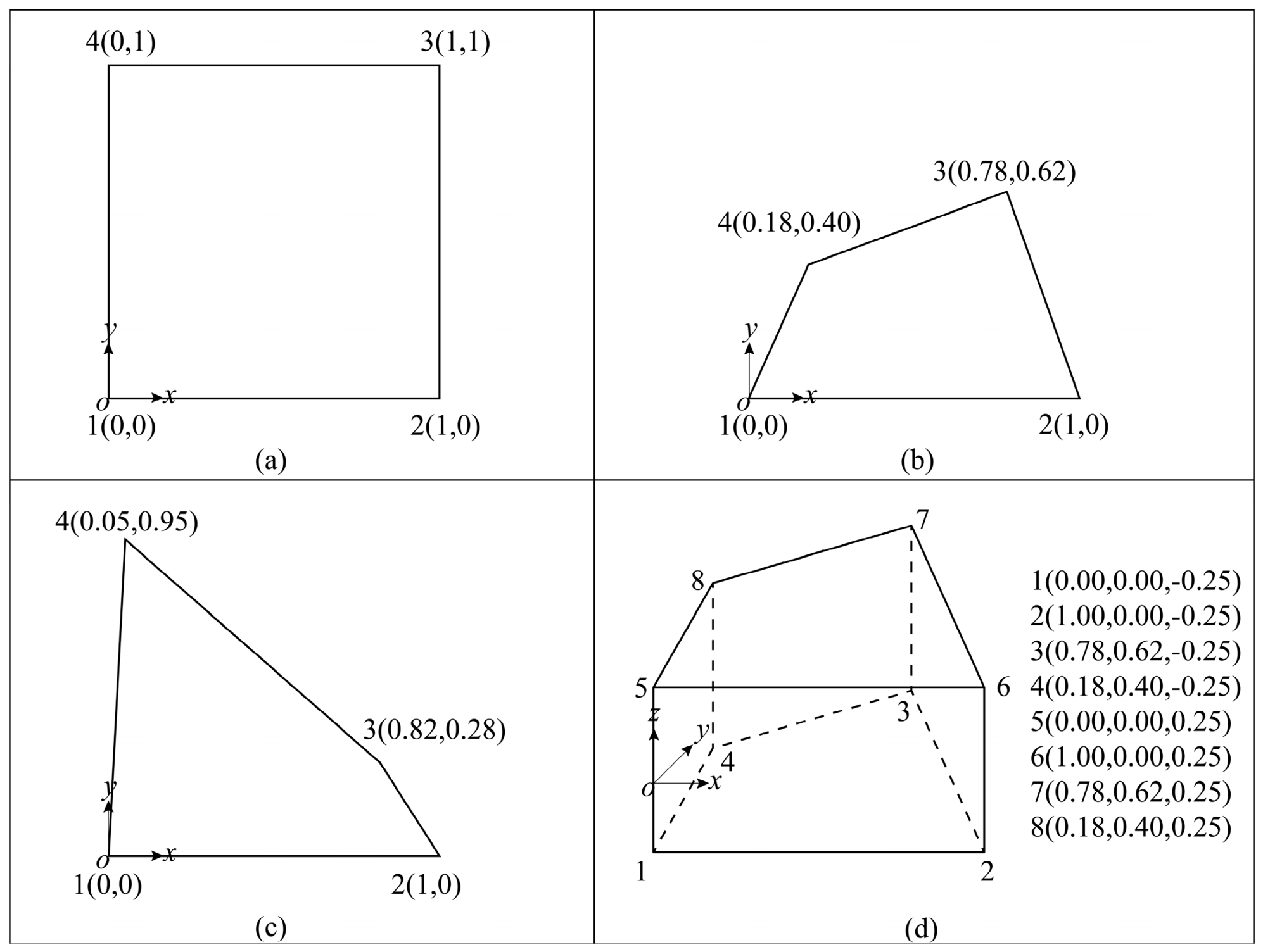
Figure 11.
First-order plane-stress patch test for the HCML-Q4, HCML-Q4R, and HCML-Q4I.
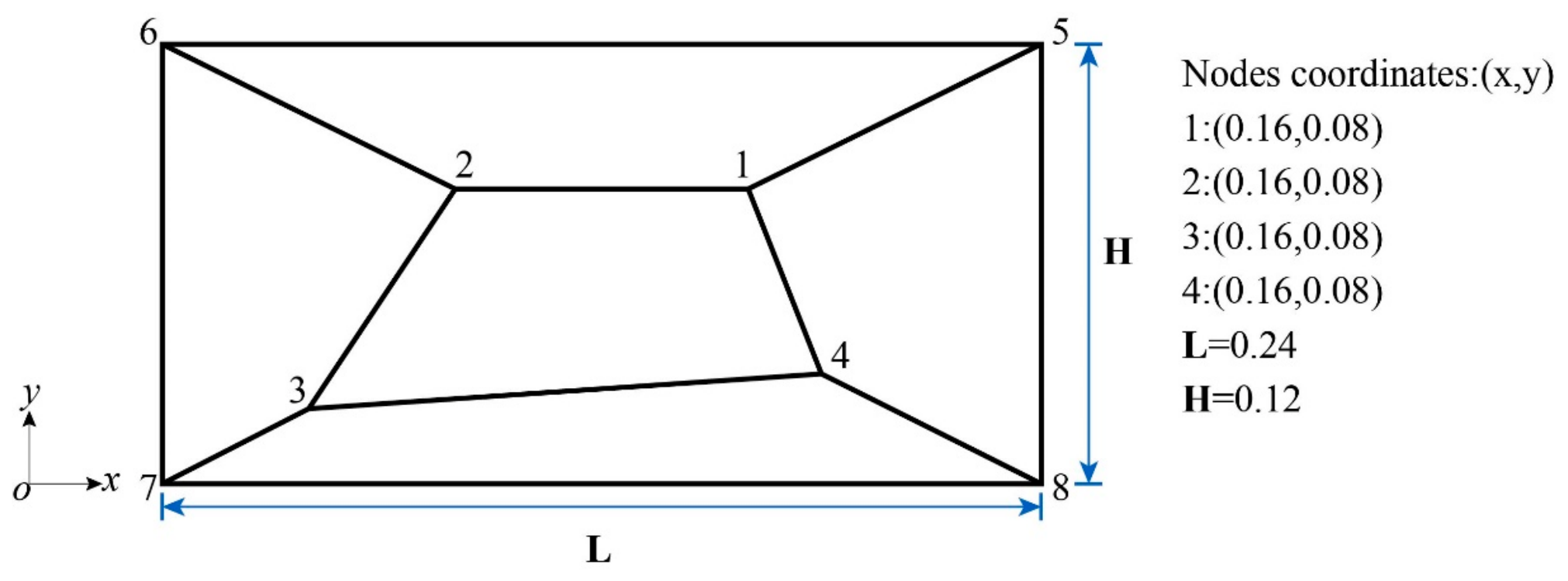
Figure 12.
Constant generalized-strain patch test for the HCML-SS8 element.
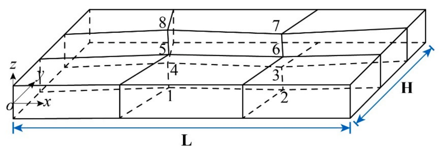
Figure 13.
MacNeal’s cantilever beam subjected to two loading cases and three mesh patterns: (a) regular (Mesh I); (b) parallelogram (Mesh II); (c) trapezoidal (Mesh III).
Figure 13.
MacNeal’s cantilever beam subjected to two loading cases and three mesh patterns: (a) regular (Mesh I); (b) parallelogram (Mesh II); (c) trapezoidal (Mesh III).
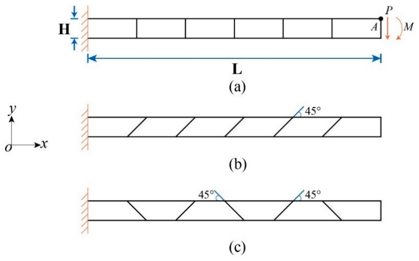
Figure 14.
Cook's skew beam: (a) geometry and boundary conditions; (b) representative mesh with and .
Figure 14.
Cook's skew beam: (a) geometry and boundary conditions; (b) representative mesh with and .
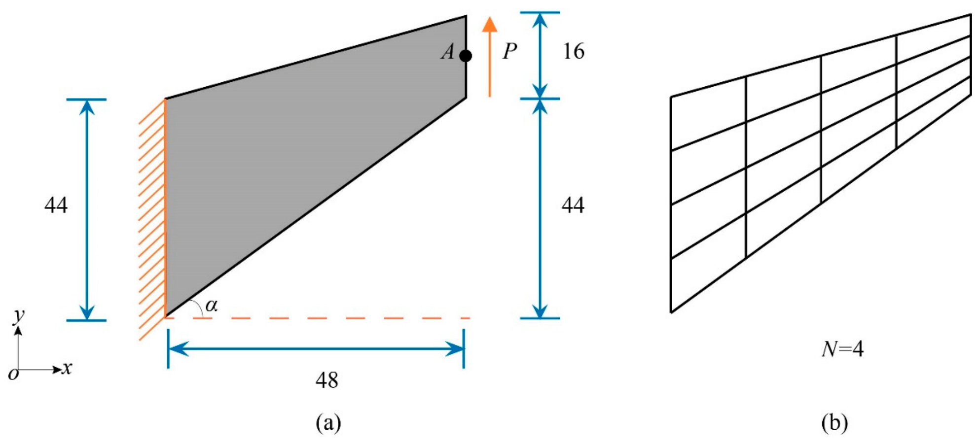
Figure 15.
Comparison of vertical displacement and von Mises stress contours obtained using Q4I and HCML-Q4I for :(a) vertical displacement of Q4I; (b) vertical displacement of HCML-Q4I; (c) von Mises stress of Q4I; and (d) von Mises stress of HCML-Q4I.
Figure 15.
Comparison of vertical displacement and von Mises stress contours obtained using Q4I and HCML-Q4I for :(a) vertical displacement of Q4I; (b) vertical displacement of HCML-Q4I; (c) von Mises stress of Q4I; and (d) von Mises stress of HCML-Q4I.
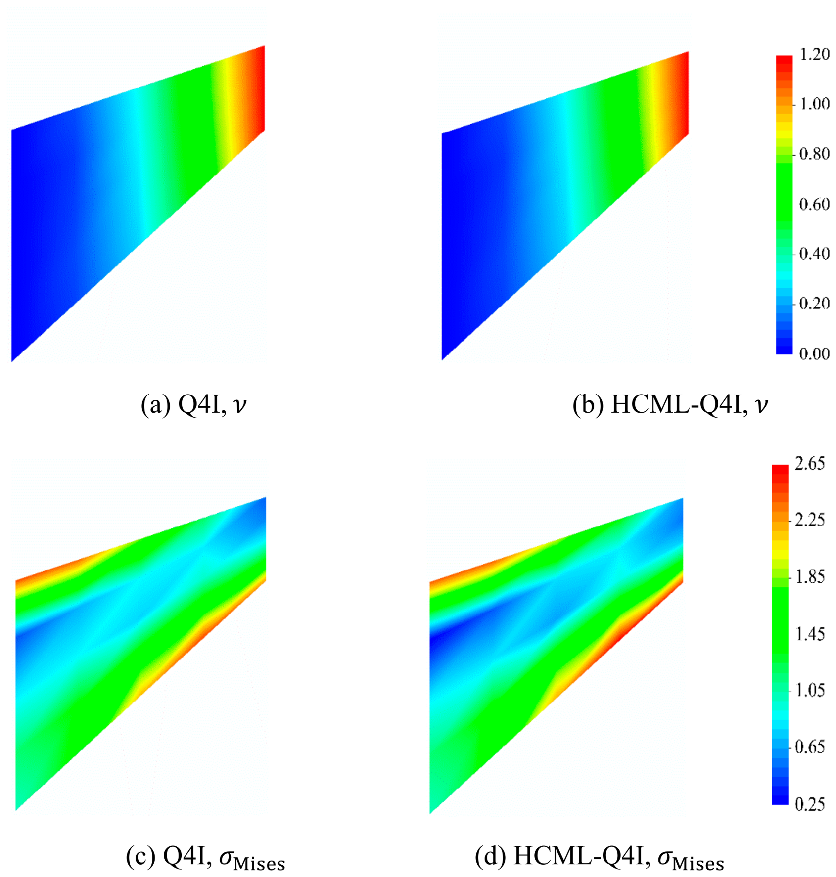
Figure 16.
Variation in the vertical displacement at point A with the geometric inclination angle .
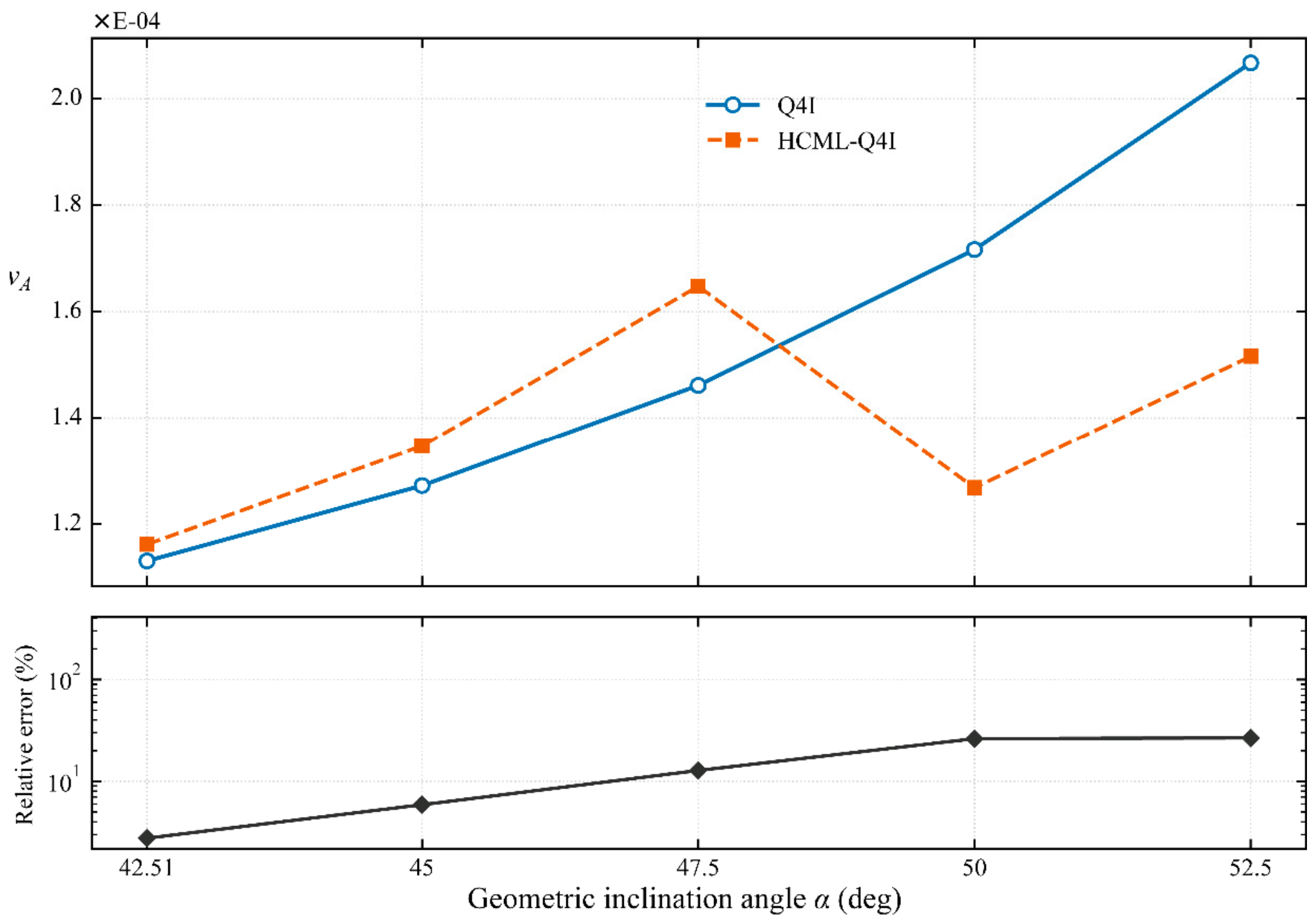
Figure 17.
Strap plate problem: (a) geometry and boundary conditions and (b), (c), (d) different mesh densities.
Figure 17.
Strap plate problem: (a) geometry and boundary conditions and (b), (c), (d) different mesh densities.
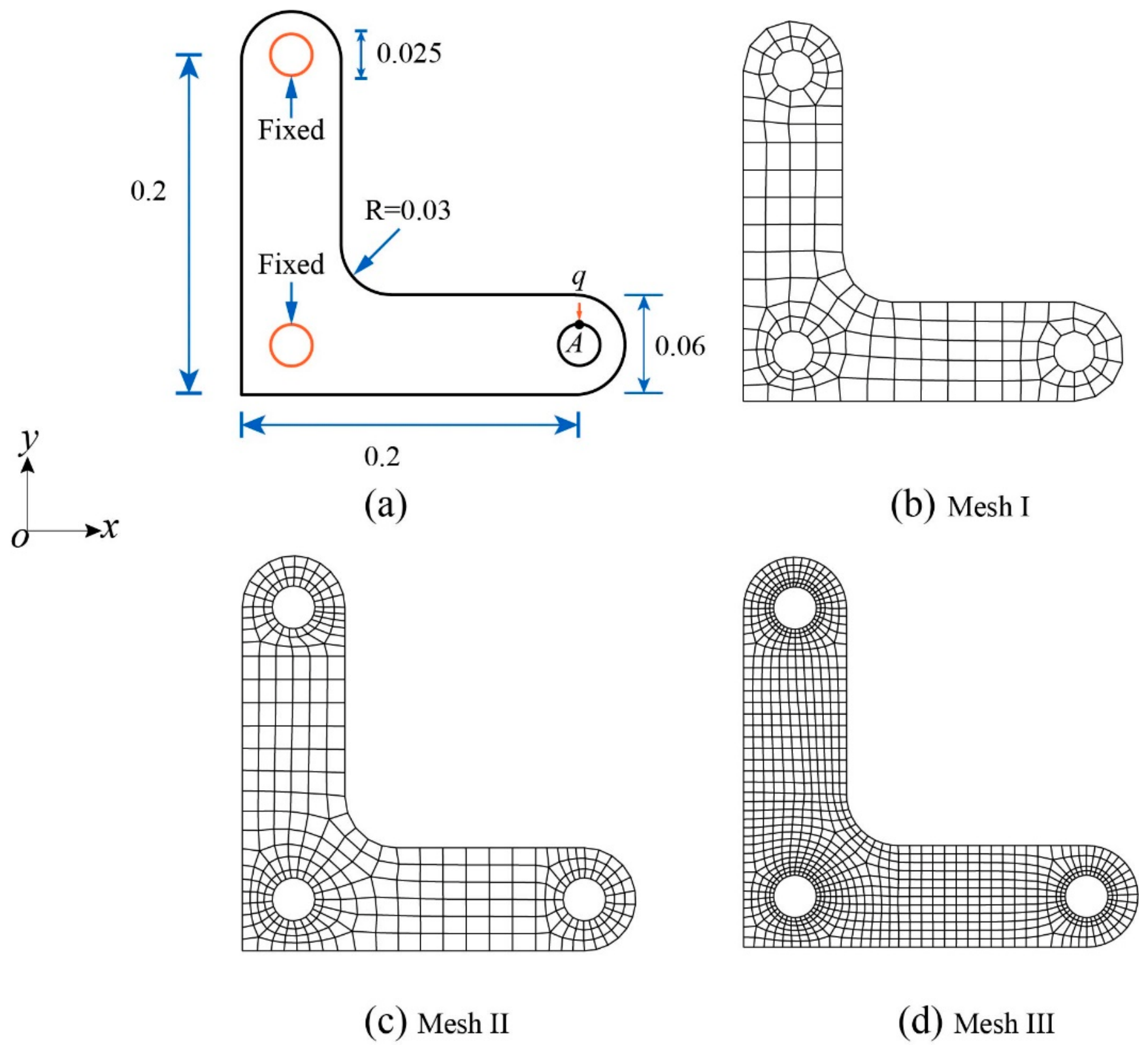
Figure 18.
Comparison of vertical displacement and von Mises stress contours obtained using Q4I and HCML-Q4I for Mesh I: (a) vertical displacement of Q4I; (b) vertical displacement of HCML-Q4I; (c) von Mises stress of Q4I; and (d) von Mises stress of HCML-Q4I.
Figure 18.
Comparison of vertical displacement and von Mises stress contours obtained using Q4I and HCML-Q4I for Mesh I: (a) vertical displacement of Q4I; (b) vertical displacement of HCML-Q4I; (c) von Mises stress of Q4I; and (d) von Mises stress of HCML-Q4I.
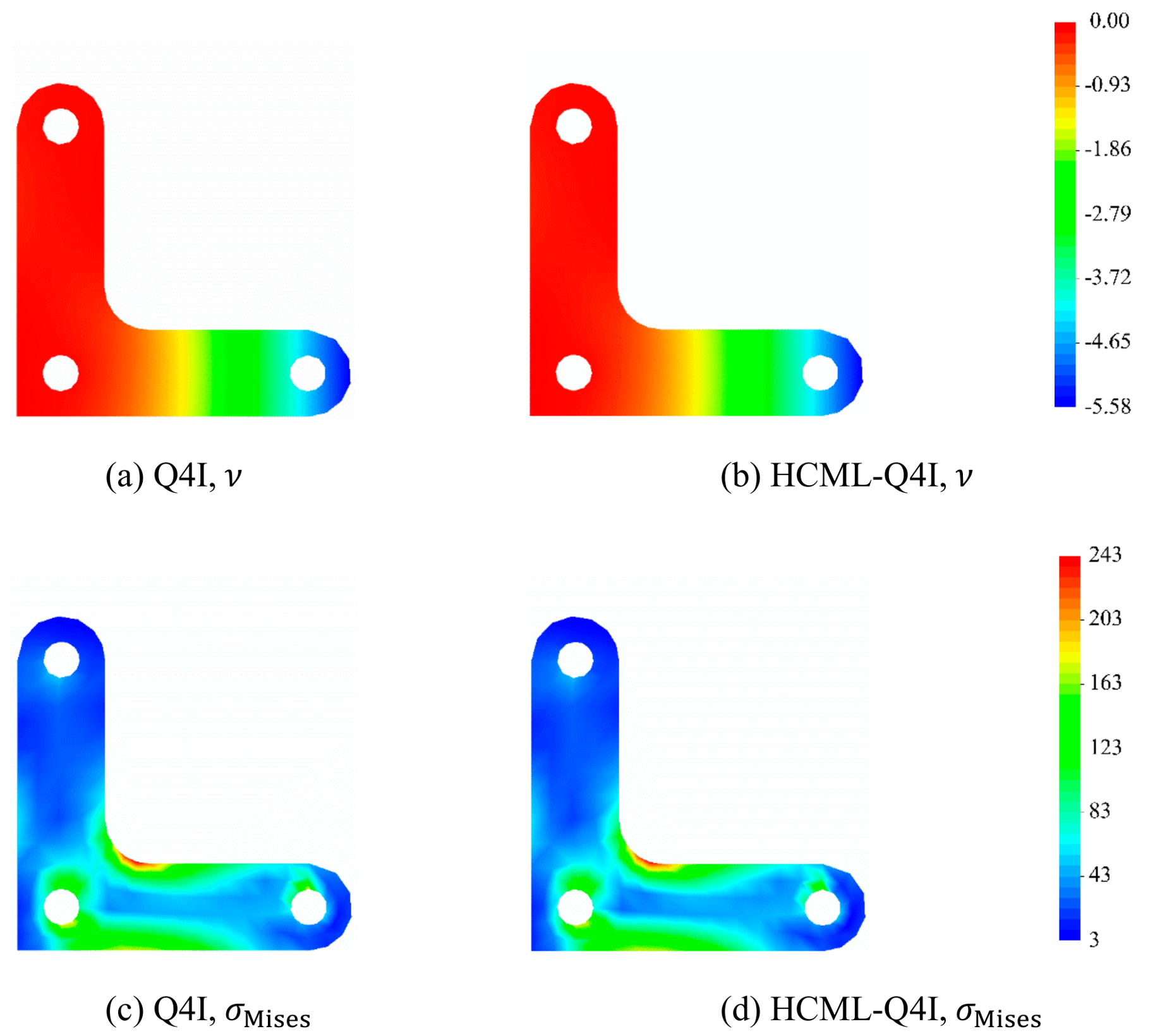
Figure 19.
Geometry, boundary conditions of the barrel vault roof.
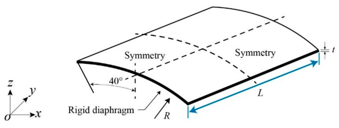
Figure 20.
Comparison of z-direction displacement and von Mises stress contours obtained using SS8 and HCML-SS8 on the 25×16×1 mesh.
Figure 20.
Comparison of z-direction displacement and von Mises stress contours obtained using SS8 and HCML-SS8 on the 25×16×1 mesh.
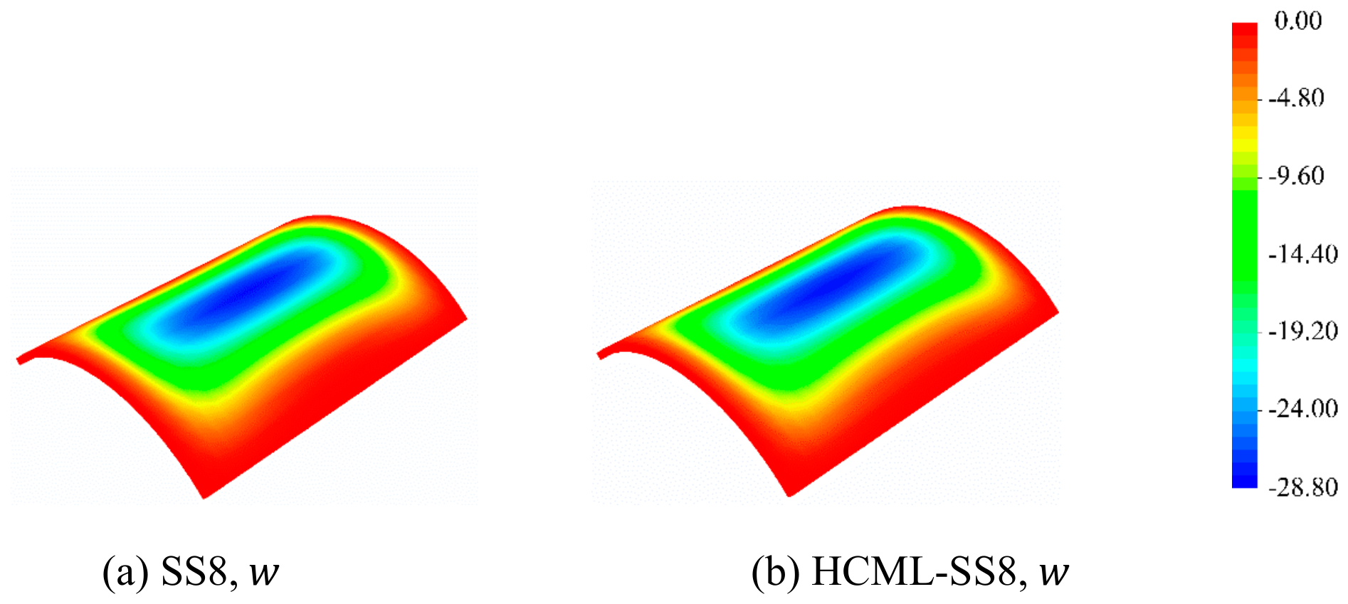
Figure 21.
Comparison of von Mises stress contours obtained using SS8 and HCML-SS8 on the 25×16×1 mesh: (a-1, b-1) top-surface von Mises stress; (a-2, b-2) midsurface von Mises stress; and (a-3, b-3) bottom-surface von Mises stress. The left and right columns correspond to SS8 and HCML-SS8, respectively.
Figure 21.
Comparison of von Mises stress contours obtained using SS8 and HCML-SS8 on the 25×16×1 mesh: (a-1, b-1) top-surface von Mises stress; (a-2, b-2) midsurface von Mises stress; and (a-3, b-3) bottom-surface von Mises stress. The left and right columns correspond to SS8 and HCML-SS8, respectively.
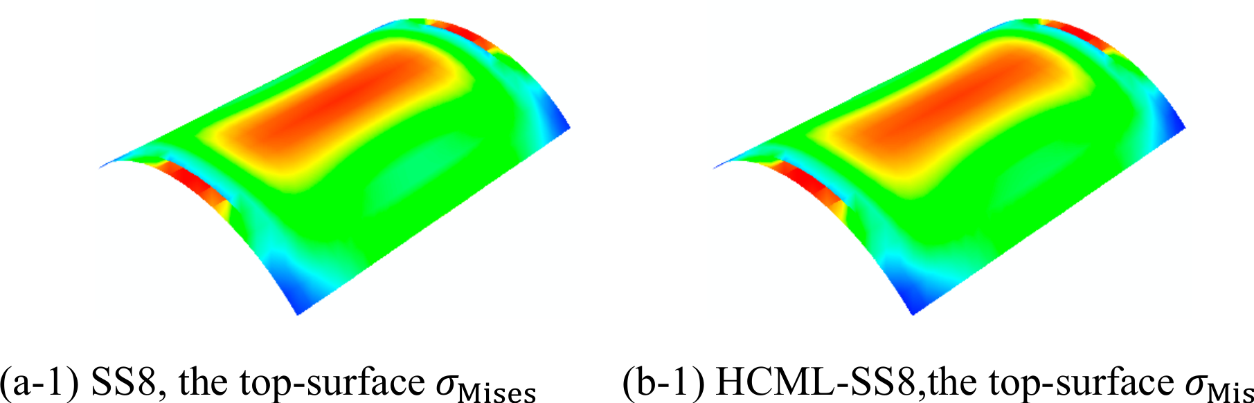
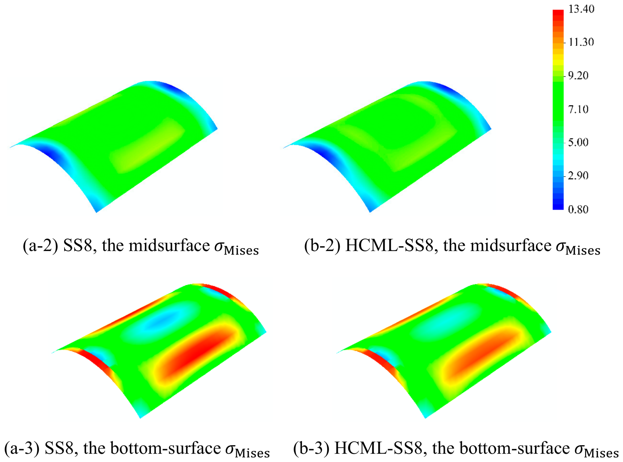
Figure 22.
Geometry, boundary conditions, and loading of the Raasch Challenge benchmark.
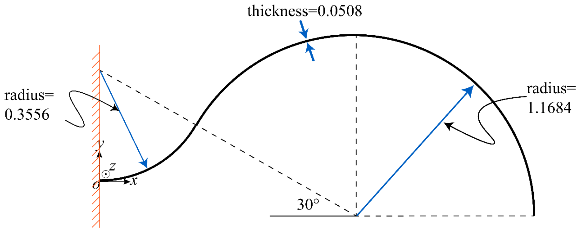
Figure 23.
Comparison of the z-direction displacement and the bottom-surface von Mises stress contours obtained using SS8 and HCML-SS8: (a) the z-direction displacement of SS8; (b) the z-direction displacement of HCML-SS8; (c) von Mises stress of SS8; and (d) von Mises stress of HCML-SS8.
Figure 23.
Comparison of the z-direction displacement and the bottom-surface von Mises stress contours obtained using SS8 and HCML-SS8: (a) the z-direction displacement of SS8; (b) the z-direction displacement of HCML-SS8; (c) von Mises stress of SS8; and (d) von Mises stress of HCML-SS8.
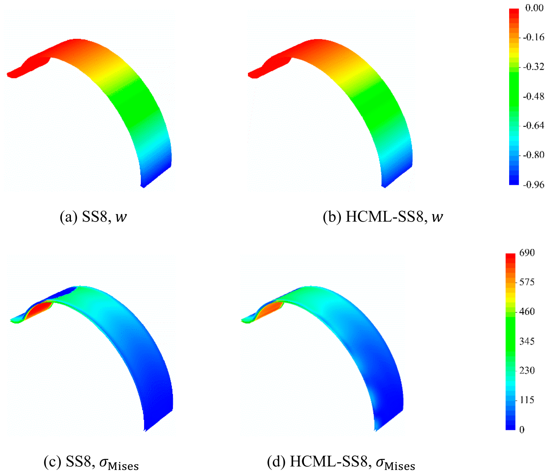
Figure 24.
Geometry, boundary conditions, and loading of the hyperbolic shell.
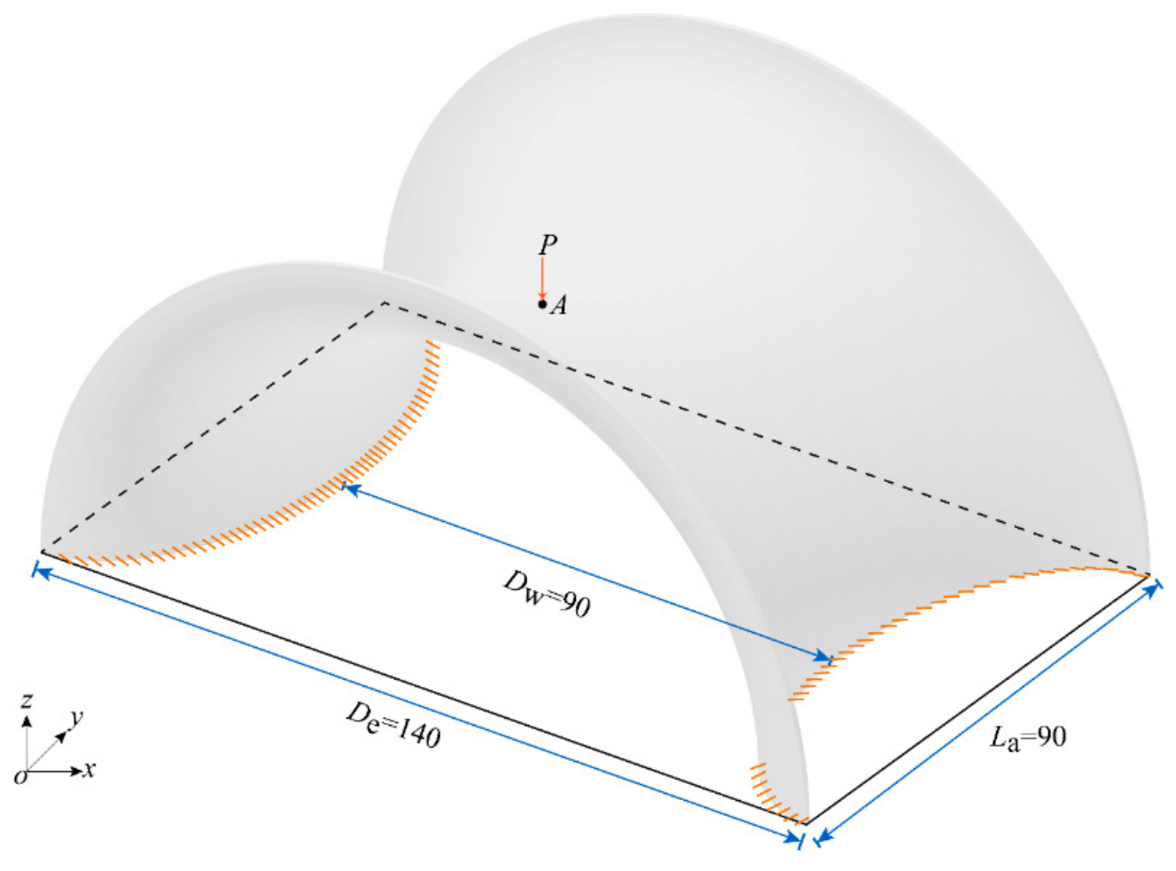
Figure 25.
Comparison of the z-direction displacement and the bottom-surface von Mises stress contours obtained using SS8 and HCML-SS8 with a single-element layer through the thickness: (a) the z-direction displacement of SS8; (b) the z-direction displacement of HCML-SS8; (c) von Mises stress of SS8; and (d) von Mises stress of HCML-SS8.
Figure 25.
Comparison of the z-direction displacement and the bottom-surface von Mises stress contours obtained using SS8 and HCML-SS8 with a single-element layer through the thickness: (a) the z-direction displacement of SS8; (b) the z-direction displacement of HCML-SS8; (c) von Mises stress of SS8; and (d) von Mises stress of HCML-SS8.
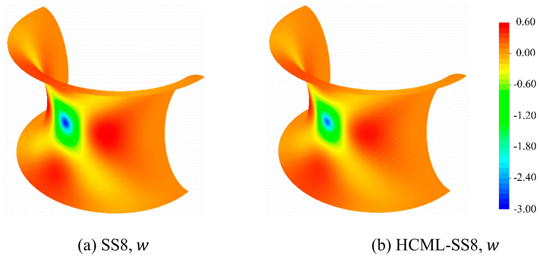
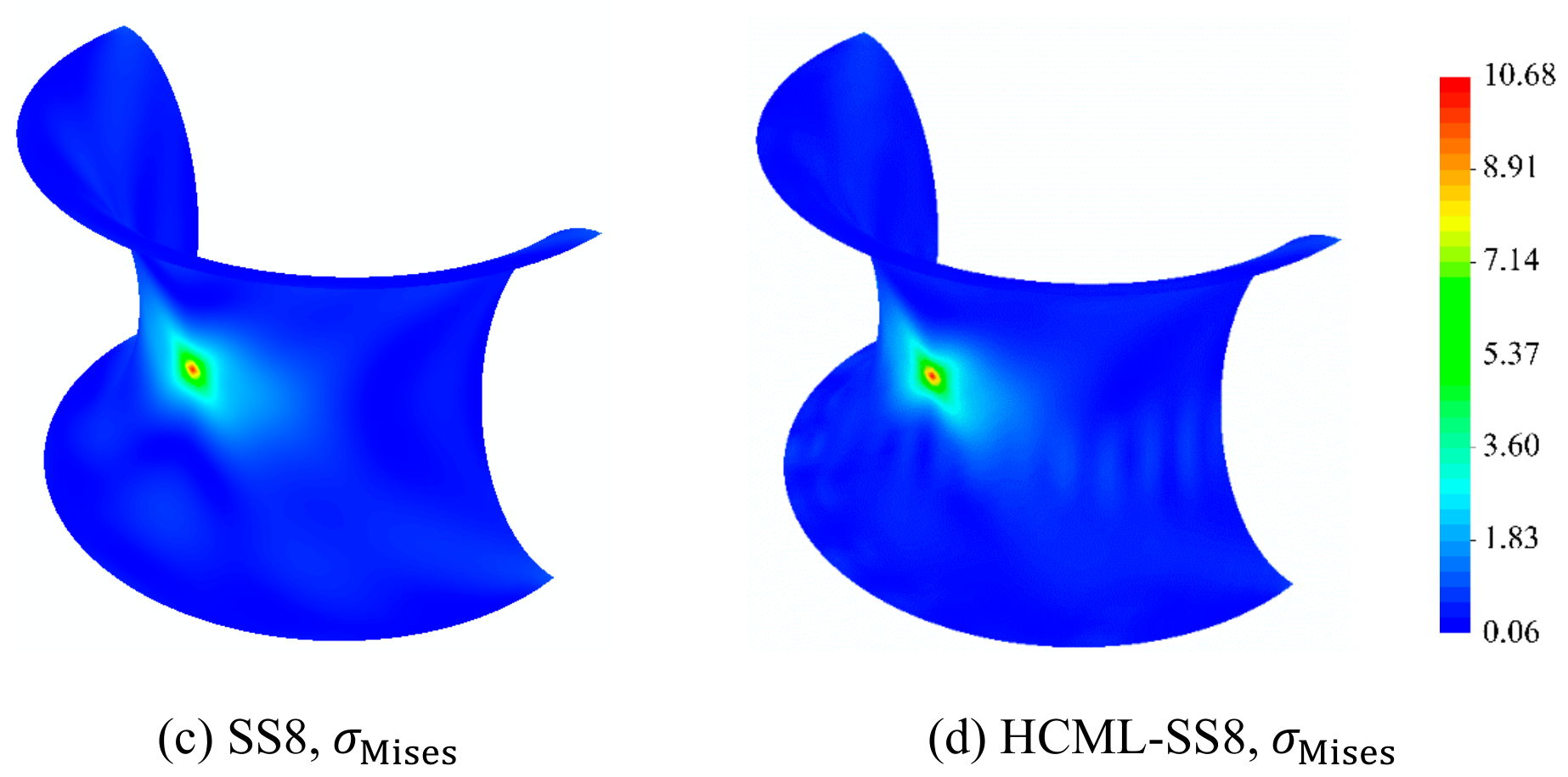
Figure 26.
Geometry, boundary conditions, and loading of the thin-walled pipe elbow with two straight sections.
Figure 26.
Geometry, boundary conditions, and loading of the thin-walled pipe elbow with two straight sections.
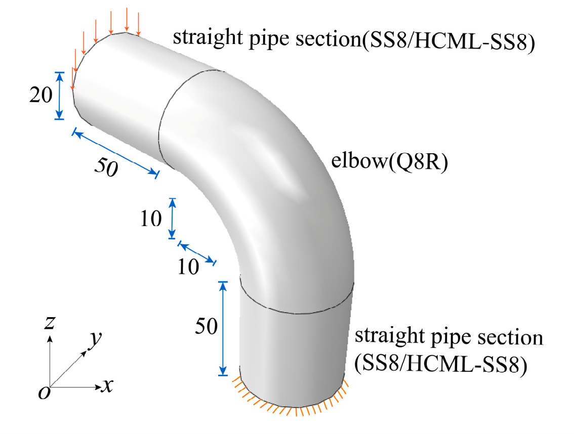
Figure 27.
Comparison of the z-direction displacement and the top-surface von Mises stress contours obtained using SS8 and HCML-SS8: (a) the z-direction displacement of SS8; (b) the z-direction displacement of HCML-SS8; (c) von Mises stress of SS8; and (d) von Mises stress of HCML-SS8.
Figure 27.
Comparison of the z-direction displacement and the top-surface von Mises stress contours obtained using SS8 and HCML-SS8: (a) the z-direction displacement of SS8; (b) the z-direction displacement of HCML-SS8; (c) von Mises stress of SS8; and (d) von Mises stress of HCML-SS8.
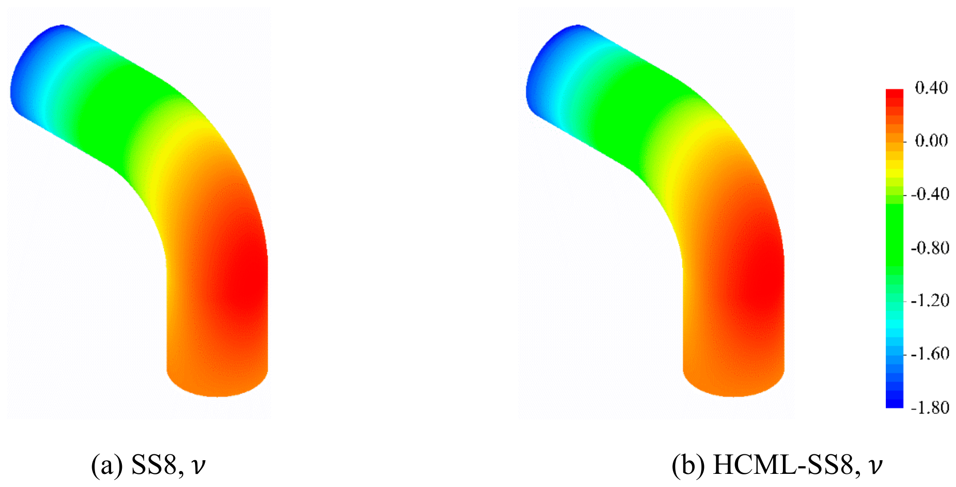
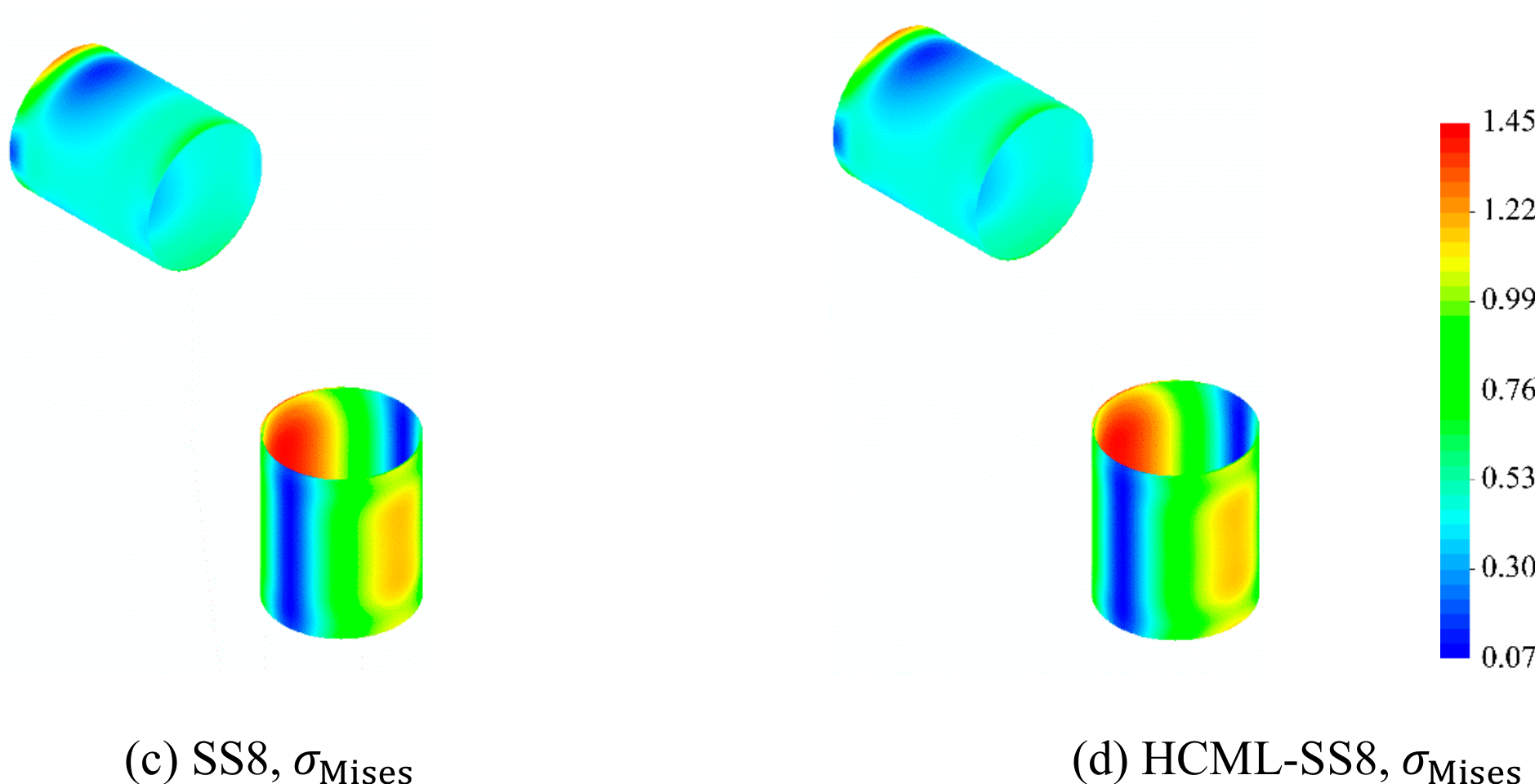

Table 1.
Element types used for numerical examples.
| Element types | Description |
|---|---|
| Q4 | Four-node bilinear plane-stress quadrilateral element with full integration |
| Q4R | Four-node bilinear plane-stress quadrilateral element with reduced integration |
| Q4I | Four-node plane-stress quadrilateral element with incompatible modes |
| Q8R | Eight-node linear brick element with reduced integration |
| SS8 | Eight-node continuum solid-shell element with reduced integration |
| HCML-Q4 | Direct data-driven element by HCML and using Q4 as training data |
| HCML-Q4R | Direct data-driven element by HCML and using Q4R as training data |
| HCML-Q4I | Direct data-driven element by HCML and using Q4I as training data |
| HCML-SS8 | Direct data-driven element by HCML and using SS8 as training data |
Table 2.
Summary of the fully connected neural-network architectures and the definitions of inputs/outputs for the two element types.
Table 2.
Summary of the fully connected neural-network architectures and the definitions of inputs/outputs for the two element types.
| Element type | Input vector | Hidden-layer widths | Output vector |
|---|---|---|---|
| HCML-Q4 variants | (Eq. (33)) | ||
| HCML-SS8 | (Eq. (49)) |
Note: The term “HCML-Q4 variants” denotes the three learned plane-stress quadrilateral elements, namely HCML-Q4, HCML-Q4R, and HCML-Q4I.
Table 3.
Rigid-body zero-energy mode test results for different HCML-FEs and representative geometric configurations.
Table 3.
Rigid-body zero-energy mode test results for different HCML-FEs and representative geometric configurations.
| Element types |
Geometry cases |
Expected / detected zero modes | Maximum absolute near-zero eigenvalue | First nonzero eigenvalue |
|---|---|---|---|---|
| HCML-Q4 | (a)/(b)/(c) | 3 / 3 for all cases | 3.444513E-10 | 6.375719E+04 |
| HCML-Q4R | (a)/(b)/(c) | 3 / 3 for all cases | 3.187618E-10 | 9.650309E+02 |
| HCML-Q4I | (a)/(b)/(c) | 3 / 3 for all cases | 3.442517E-10 | 4.162220E+03 |
| HCML-SS8 | (d) | 6 / 6 | 1.979137E-09 | 1.507238E+02 |
| Q4-Soft | (a)/(b)/(c) | 3 / 0 for all cases | 3.388309E+04 | 8.122233E+04 |
Table 4.
Interior nodal displacement components in the first-order plane-stress patch test for HCML-FEs.
Table 4.
Interior nodal displacement components in the first-order plane-stress patch test for HCML-FEs.
| Nodes | Analytical displacements | HCML-FE displacements () |
|---|---|---|
| 1 | (2.00000000,1.60000000) | (2.00000000,1.59999999) |
| 2 | (1.20000000,1.20000000) | (1.20000000,1.19999998) |
| 3 | (5.00000000,4.00000000) | (5.00000006,4.00000002) |
| 4 | (1.95000000,1.20000000) | (1.94999999,1.20000000) |
Table 5.
Interior nodal displacement components in the constant generalized-strain patch test.
| Nodes | Analytical displacements | HCML displacements |
|---|---|---|
| 1 | (-1.05000, -0.90000, -6.45000) | ( -1.05000, -0.89999, -6.44999) |
| 2 | (-1.80000, -1.20000, -16.80000) | (-1.80000, -1.20000, -16.80000) |
| 3 | (-1.95000, -1.65000, -22.05000) | (-1.95000, -1.65000, -22.05000) |
| 4 | (-1.20000, -1.35000, -10.95000) | (-1.20000, -1.35000, -10.95000) |
| 5 | (1.05000, 0.90000, -6.45000) | (1.05000, 0.89999, -6.44999) |
| 6 | (1.80000, 1.20000, -16.80000) | (1.80000, 1.20000, -16.80000) |
| 7 | (1.95000, 1.65000, -22.05000) | (1.95000, 1.65000, -22.05000) |
| 8 | (1.20000, 1.35000, -10.95000) | (1.19999, 1.35000, -10.95000) |
Table 6.
Vertical displacement at point A for two load cases and three mesh patterns: comparison between reference elements and HCML-FEs.
Table 6.
Vertical displacement at point A for two load cases and three mesh patterns: comparison between reference elements and HCML-FEs.
| Elements | Load | Load | ||||
|---|---|---|---|---|---|---|
| Mesh I | Mesh II | Mesh III | Mesh I | Mesh II | Mesh III | |
| Q4 | -0.930 | -0.375 | -0.359 | -0.046 | -0.016 | -0.015 |
| HCML-Q4 | -0.881 | -0.398 | -0.356 | -0.044 | -0.01756 | -0.0153 |
| Q4R | -364.5 | -108.0 | -40.38 | -18.350 | -4.931 | -0.997 |
| HCML-Q4R | -150.8 | -0.851 | -25.25 | -7.593 | -0.0243 | -0.2886 |
| Q4I | -1.999 | -1.676 | -0.526 | -0.100 | -0.0872 | -0.0218 |
| HCML-Q4I | -1.976 | -1.583 | -0.528 | -0.0988 | -0.0807 | -0.0214 |
| Reference solutions:-2.000 for load and -0.100 for load | ||||||
Table 7.
The vertical displacement by HCML and reference elements for different mesh densities when .
Table 7.
The vertical displacement by HCML and reference elements for different mesh densities when .
| Elements | ||||||
|---|---|---|---|---|---|---|
| Q4 | 0.2959 | 0.5837 | 0.9007 | 1.085 | 1.152 | 1.172 |
| HCML-Q4 | 0.3104 | 0.6070 | 0.9209 | 1.107 | 1.158 | 1.174 |
| Q4R | 0.2959 | 1.334 | 1.220 | 1.189 | 1.182 | 1.181 |
| HCML-Q4R | 0.9043 | 1.632 | 1.261 | 1.225 | 1.191 | 1.183 |
| Q4I | 0.7256 | 0.9976 | 1.131 | 1.164 | 1.175 | 1.178 |
| HCML-Q4I | 0.9521 | 1.152 | 1.162 | 1.199 | 1.185 | 1.183 |
| Reference solutions: | ||||||
Table 8.
Maximum vertical nodal displacement computed by HCML-FEs and reference elements for the strap plate problem under different mesh densities.
Table 8.
Maximum vertical nodal displacement computed by HCML-FEs and reference elements for the strap plate problem under different mesh densities.
| Elements | |||
|---|---|---|---|
| Q4 | -5.112 | -5.224 | -5.344 |
| HCML-Q4 | -5.113 | -5.224 | -5.343 |
| Q4R | -5.649 | -5.562 | -5.460 |
| HCML-Q4R | -5.577 | -5.506 | -5.416 |
| Q4I | -5.257 | -5.332 | -5.372 |
| HCML-Q4I | -5.526 | -5.323 | -5.373 |
| Reference solutions: | |||
Table 9.
Relative errors in the maximum z-direction displacement between HCML-SS8 and SS8 for different mesh densities.
Table 9.
Relative errors in the maximum z-direction displacement between HCML-SS8 and SS8 for different mesh densities.
| Mesh | Err (%) |
|---|---|
| 25×16×1 | 5.23 |
| 50×32×2 | 0.13 |
Table 10.
Comparison of the maximum nodal displacement in the z-direction obtained by SS8 and HCML-SS8 with different mesh densities.
Table 10.
Comparison of the maximum nodal displacement in the z-direction obtained by SS8 and HCML-SS8 with different mesh densities.
| Elements | 70×54×1 mesh | 140×108×2 mesh | ||
|---|---|---|---|---|
| Err (%) | Err (%) | |||
| SS8 | -2.95 | 7.46 | -2.92 | 4.80 |
| HCML-SS8 | -2.73 | -2.78 | ||
Table 11.
Statistics of thickness-edge deviation angles for the solid-shell examples.
| Example | Mean thickness-edgedeviation angle () | Maximum thickness-edge deviation angle () |
|---|---|---|
| Barrel Vault Roof | 2.81 | 2.81 |
| Raasch Challenge | 0.73 | 1.82 |
| Hyperboloid Shell | 15.17 | 25.90 |
Disclaimer/Publisher’s Note: The statements, opinions and data contained in all publications are solely those of the individual author(s) and contributor(s) and not of MDPI and/or the editor(s). MDPI and/or the editor(s) disclaim responsibility for any injury to people or property resulting from any ideas, methods, instructions or products referred to in the content. |
© 2026 by the authors. Licensee MDPI, Basel, Switzerland. This article is an open access article distributed under the terms and conditions of the Creative Commons Attribution (CC BY) license (http://creativecommons.org/licenses/by/4.0/).
Copyright: This open access article is published under a Creative Commons CC BY 4.0 license, which permit the free download, distribution, and reuse, provided that the author and preprint are cited in any reuse.