
Submitted:
04 September 2026
Posted:
07 September 2026
You are already at the latest version
Abstract
We prove, to our knowledge, the first unconditional cumulative closure estimates for the Arnold-Mukherjee-Pouly (AMP) refinement algorithm and the original face-marked tetrahedral algorithm of Bänsch on arbitrary conforming initial tetrahedral meshes. Let \( \mathcal T_0,...,\mathcal T_L \) be an adaptive mesh sequence generated by either algorithm, with \( \mathcal{M}_\ell\subseteq\mathcal{T}_\ell \) denoting the marking set at step \( \ell \). Then \( \#\mathcal{T}_L-\#\mathcal{T}_0\le C_{\mathrm{clos}}(\mathcal{T}_0)\sum_{\ell=0}^{L-1}\#\mathcal{M}_\ell \). The proof organizes conformity refinements into a causal forest and combines a uniform horizontal-propagation estimate with a weighted packing argument to obtain an explicit closure constant. For the original Bänsch algorithm, every history-dependent resolution of the initial two-edge ambiguity is represented by an AMP history associated with one of finitely many initial resolutions. The estimate therefore holds uniformly for arbitrary deterministic or nondeterministic choices. This resolves a long-standing complexity question for the Bänsch-AMP family.
Keywords:
etrahedral bisection
; Arnold–Mukherjee–Pouly algorithm
; Bänsch algorithm
; closure complexity estimate
; horizontal propagation
; adaptive finite element method
MSC: 65N50; 65Y20; 65N30
1. Introduction
Adaptive finite element methods (AFEMs) rely on local mesh refinement to concentrate computational effort near singularities, layers, interfaces, and other fine-scale features. A standard adaptive feedback loop is of the form
Convergence and optimality of AFEMs have been established in [4,6,7,9,21,27]. Besides conformity and uniform shape regularity, optimal complexity of AFEMs requires the Refine routine to satisfy a quantitative complexity property. In particular, conforming completion may create more elements than were explicitly marked, but its cumulative overhead must remain proportional to the cumulative number of marked elements. Let be the marking set at the ℓth AFEM iteration, namely the set of elements selected for refinement, and
be a sequence of locally refined meshes output by an AFEM. The desired closure estimate has the form
This closure estimate is one of the foundations of rate-optimal AFEM theory [4,5,28]. In three dimensions, its proof is particularly delicate because one bisection may launch a long chain of conformity refinements through faces and edge stars, and repeated calls may revisit the same physical region at many scales.
In modern AFEMs, bisection has become a standard local-refinement mechanism because it preserves nestedness and reduces mesh management to a small number of local operations. For triangular meshes, longest-edge bisection [23,24,25,29] and newest-vertex bisection [19,20,26] are the predominant bisection algorithms. The passage to tetrahedral and simplicial meshes produced several distinct refinement paradigms. Bänsch proposed a face-marked bisection method with an ambiguity in two and three dimensions [3] that works on arbitrary initial meshes. Arnold–Mukherjee–Pouly (AMP) later recast the Bänsch rule in a particularly transparent marked-tetrahedron data structure and proved conformity, termination, and finitely many similarity classes [2]. Other related tetrahedral approaches include the Liu–Joe bisection framework [16,17] and the skeleton-based refinement strategy of Plaza and Carey [22].
In a different paradigm, Kossaczký developed a recursive newest-vertex-type construction in two and three dimensions under restrictions on the initial mesh [14]. Maubach and Traxler extended this construction to arbitrary dimension by assigning an ordered vertex list to every simplex, which hinges on compatibility across neighboring simplices and imposes a structural condition on the coarse mesh [18,30]. By contrast, Bänsch–AMP is face-based: the input data are edge marks intrinsic to the triangular faces, and in three dimensions these marks can be initialized directly on any conforming tetrahedral mesh from a single global edge order, without a compatible simplex-ordering construction.
Closure complexity estimates for bisection algorithms developed along a somewhat different line. Binev, Dahmen, and DeVore [4] proved the decisive cumulative estimate for two-dimensional newest vertex bisection under an initial compatibility condition. Stevenson extended such estimates to Traxler’s algorithm in arbitrary dimension under a matching-neighbor condition [28]. In two dimensions, Karkulik, Pavlicek, and Praetorius proved that newest vertex bisection satisfies (1) on every conforming initial triangular mesh, without any compatibility assumption [12,13]. Recently, the authors proved the same closure estimate for the longest edge bisection on arbitrary triangular meshes [15].
In dimensions higher than two, the usual matching-neighbor assumptions needed by Traxler’s algorithm may not hold on general triangulations. Alkämper–Gaspoz–Klöfkorn (AGK) introduced a weak compatibility condition and a linear-time relabeling procedure that ensures termination of iterative refinement in arbitrary dimension [1]. Gehring subsequently proved (1) for every initial labeling produced by the AGK initialization algorithm [10]. Most recently, Diening–Gehring–Storn (DGS) supplied the Maubach routine with an initialization valid for every conforming initial triangulation and proved closure by relating the physical mesh to a suitably colored triangulation in a higher-dimensional space [8].
Existing closure complexity analyses follow the line of Maubach–Traxler. On the other hand, the Bänsch–AMP family occupies a distinctive place in this history. The Bänsch algorithm, introduced in 1991, acts directly on a given conforming tetrahedral mesh, without a coloring or matching-neighbor assumption [3]. The AMP algorithm is its later finite-state realization. Indeed, every initial mesh can be initialized by marking each face with its maximal edge in one global edge order. Thus no preliminary refinement or global compatibility construction is required. This unusually simple initialization is one of the principal advantages of Bänsch–AMP.
Despite that early generality, the Bänsch–AMP closure complexity of the form (1) has remained an open question since the original works [2,3]. The present manuscript resolves this long-standing problem in modern AFEM optimality theory. To our knowledge, it gives the first unconditional cumulative closure estimates for Bänsch and AMP on arbitrary conforming initial tetrahedral meshes, including the nondeterministic choice allowed by the original Bänsch formulation. The proof is intrinsic to the physical three-dimensional mesh: it uses neither a higher-dimensional embedding nor an initial compatibility hypothesis. The proof requires a new causal analysis of conformity propagation rather than a direct application of classical newest-vertex-bisection completion theory.
The main contributions are the following.
- (i)
- We construct intrinsic marked-face refinement trees and a causal forest for conformity events. The construction gives the macro-generation monotonicity needed to control propagation. A finite analysis of the five physical edge classes, two transition tables, and vertex- and edge-star bounds then proves uniform horizontal propagation within a fixed macro-generation. Writing for the resulting uniform macro-vertex valence, the bound is
- (ii)
- We convert horizontal boundedness into geometric locality by showing that every causal descendant remains in a controlled same-scale neighborhood of its root event. Let and denote, respectively, the lower volume-scale and upper diameter-scale constants from Lemma 1. An optimized self-contained weighted packing argument then charges the resulting refinement cost to the marked elements and yields
- (iii)
- We resolve the two-edge choice in the original Bänsch formulation. Every Bänsch child has a unique global refinement edge, and a deferred-resolution argument represents every history-dependent Bänsch history by an AMP history associated with one of finitely many initial resolutions. The AMP closure estimate therefore transfers uniformly to arbitrary deterministic or nondeterministic choices.
The result is three-dimensional: both the AMP marking rules and the finite transition analysis are specific to tetrahedra. sec:amp-algorithm restates the algorithm and its three-bisection macrostructure. sec:amp-analysis develops the intrinsic causal structure. sec:horizontal-propagation proves the horizontal-propagation bound by a finite macrostep analysis, and sec:amp-closure derives locality and closure from that bound. Finally, sec:bansch-analysis states the Bänsch rules intrinsically and derives the uniform closure consequence. sec:numerics reports the numerical experiments.
2. The AMP Refinement Algorithm
This section fixes the AMP data structure and refinement rules used throughout the paper. The material is restated from Arnold–Mukherjee–Pouly [2], with notation adapted to the present analysis. Their marked-tetrahedron formulation is essentially equivalent to the earlier face-marked algorithm of Bänsch once one refinement edge is selected in the ambiguous two-edge case. We return to the original Bänsch formulation in sec:bansch-analysis.
2.1. Tetrahedral Meshes and Marked Tetrahedra
Let be an arbitrary conforming tetrahedral triangulation of a polyhedral domain . A tetrahedral mesh is a finite collection of closed tetrahedra such that distinct tetrahedra have disjoint interiors and . For a tetrahedron or a mesh X, write , , and for its sets of vertices, edges, and faces. The mesh is conforming if the intersection of two distinct tetrahedra is empty or is a common vertex, a common edge, or a common face.
Definition 1
(Marked tetrahedron). A marked tetrahedron K consists of its four vertices, a refinement edge , a marked edge for every , and a Boolean flag. The two faces containing are therefinement faces, and on each of them . The remaining two faces are thenonrefinement faces. The flag may be set only when the four face marks are coplanar.
The marked edges of the two nonrefinement faces are each either adjacent or opposite to the refinement edge. This gives the AMP types:
- type P (planar), if all face marks are coplanar; the type is denoted by or according as the flag is unset or set;
- type A (adjacent), if the marked edges of both nonrefinement faces meet the refinement edge but the four marks are not coplanar;
- type O (opposite), if neither nonrefinement face has its marked edge meeting the refinement edge;
- type M (mixed), if the marked edge of exactly one nonrefinement face meets the refinement edge.
Thus is the only type whose flag is set; the flags of , and M are unset. Figure 1 displays one representative of each type both as a marked tetrahedron and as an unfolded face net.
An AMP marked mesh is a tetrahedral mesh whose tetrahedra carry the marked-tetrahedron structure of def:markedtetrahedron. We use the same symbol for the marked mesh and its underlying tetrahedral collection whenever only membership or cardinality is concerned. It is conformingly marked if its underlying mesh is conforming and the markings induced by two incident tetrahedra on any shared face F agree; that is, both assign the same edge to F.
2.2. The Marked Tetrahedron Bisection
Fix with refinement edge , and write . In the rules below, an inherited face is a face of K, a cut face is a proper subtriangle of a face of K, and the new face common to the children is .
- (B1)
- The inherited face keeps its marked edge from K; this edge is the refinement edge of the child.
- (B2)
- A cut face is marked by its edge opposite the new vertex m.
- (B3)
- The common new face is marked by the edge opposite the new vertex m, except when K is of type ; then it is marked by , where is the common old endpoint of the two child refinement edges.
- (B4)
- The child flags are set if and only if K is of type .
Figure 2.
Bisection of a tetrahedron along its refinement edge. The dashed segments from m are the new edges; the two children share the new face .
Figure 2.
Bisection of a tetrahedron along its refinement edge. The dashed segments from m are the new edges; the two children share the new face .
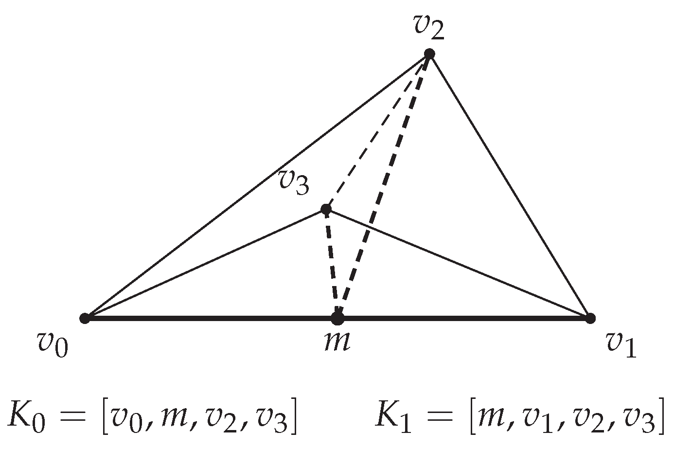
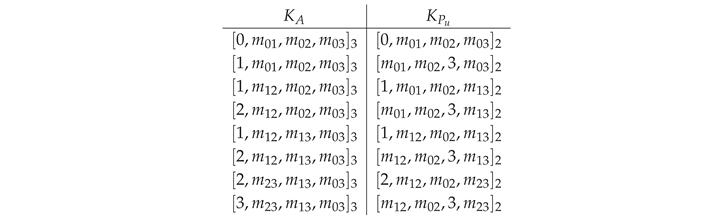
For an explicit instance of the four rules, take a type- tetrahedron with unset flag and face marks
The child data are listed in Table 1.
Both children have the same type. The complete type transition is shown in Figure 3. In particular, types M and O occur only in the initial transient.
Repeated bisection organizes the descendants of each initial tetrahedron into a binary refinement tree. The generation of a descendant K is its depth in this tree, namely the number of bisections from its unique ancestor in . Thus every bisection increases generation by one and halves volume. At an intermediate stage, an active tetrahedron is a leaf of one of these trees: it has been created and has not itself been bisected. The active tetrahedra form the current, possibly nonconforming, mesh . A current mesh vertex is a hanging vertex of an active tetrahedron if
Equivalently, z lies in the relative interior of an edge or a face of K; an arbitrary point there is not a hanging vertex.
In Figure 4, and the two children of are all active, but only has m as a hanging vertex. Hence , but neither child of , is selected for bisection in the next step of conformity completion.
2.3. Conforming Initialization and Local Refinement
An initial AMP marked mesh is a finite conformingly marked AMP mesh whose flags are all unset. A convenient canonical initialization imposes one strict global order on all edges of . The maximal edge of each tetrahedron is its refinement edge, the maximal edge of each face is its marked edge, and every flag is unset. A shared face therefore receives the same mark from both sides. No coloring or matching-neighbor condition is imposed on . Henceforth, dependence on an initial AMP marked mesh includes its fixed refinement edges, face marks, and flags; the global edge order is only one way to construct these data.
Let be a current AMP marked mesh and let . We write BisectTets for the routine that replaces every tetrahedron of by the two children returned by Algorithm 1; all other tetrahedra are unchanged.
| Algorithm 1:One AMP marked-tetrahedron bisection BisectTet |
|
Input: A marked tetrahedron K with refinement edge
Output: the two marked children
and Assign marks and flags according to (B1)–(B4) return
|
|
Algorithm 2: Simultaneous AMP bisection BisectTets
|
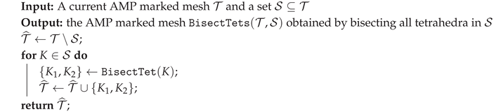 |
The AMP local-refinement procedure [2] is summarized in Algorithm 3. We call each application of BisectTets a bisection batch. In one RefineAMP call, the first batch, which bisects the marking set, is batch zero; every subsequent batch within RefineToConformity is a conformity batch.
| Algorithm 3:One AMP refinement call RefineAMP |
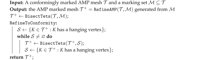 |
Thus the input–output map of Algorithm 3 is
Despite its name, the RefineToConformity module need not return a conforming mesh for an arbitrary marked input: in three dimensions, a mesh without hanging vertices may still be nonconforming. However, thm:AMPtermination shows that the recursive AMP refinement procedure starting from an initial AMP marked mesh is well defined: every call terminates and returns a conformingly marked AMP mesh.
Theorem 1
(AMP termination and conformity). Let be an initial AMP marked mesh. For arbitrary marking sets , the recursion
is well defined: every call terminates and returns a conformingly marked AMP mesh. Moreover, every tetrahedron of has generation at most .
Proof.
This is the termination and generation theorem of Arnold–Mukherjee–Pouly [2]. □
2.4. The Three-Bisection Macrostructure
Let be the mesh obtained by applying uniformly times to every initial tetrahedron. We call the qth macro-mesh. The AMP three-bisection structure partitions the geometric edges occurring in the uniform refinement tree into the sets , , see [2]. We call q the macro-generation of an edge and write
We call the passage from to one AMP macrostep. For a tetrahedron K, we set the level of K as
If , , we call s the microgeneration of K.
Proposition 1
(AMP macrostructure). The uniform AMP refinement tree has the following properties.
- (A1)
- Every is conformingly marked and unflagged. For , each tetrahedron of is of type A or .
- (A2)
- If , , then the possible types of K and the macro-generations of its edges are

- (A3)
- The descendants of the fixed finite initial mesh belong to finitely many similarity classes and are uniformly shape regular.
Proof.
Items (A1)–(A2) are proved in [2, Lemmas 3.2–3.3 and Proposition 3.4]. Item (A3) follows from the finite-similarity-class theorem; see [2, Proposition 4.1 and Theorems 4.2 and 4.5]. □
3. Intrinsic Causal Structure
The algorithm and macrostructure recalled in the preceding section are due to Arnold–Mukherjee–Pouly. We now derive the intrinsic refinement trees and causal chains associated with one refinement call and prove their macro-generation monotonicity, together with the macro-star counting consequences used below. The resulting horizontal-propagation bound is proved in sec:horizontal-propagation; its consequences for geometric locality and closure complexity are developed in sec:amp-closure.
3.1. Geometry of AMP Descendants
By the shape-regularity statement in prop:AMPmacrostructure, the descendants of the fixed finite initial mesh are uniformly shape regular, with constants depending only on and its initial markings.
Lemma 1
(Scale bounds). There are constants , depending only on the fixed initial mesh , such that every AMP descendant K satisfies
Proof.
Let be the ancestor of K and write with . Since each bisection halves volume,
For a vertex and an edge , set
Lemma 2
(Uniform vertex and edge valence). The quantity
Moreover, it holds that
Proof.
The AMP finite-similarity-class property ensures uniform shape regularity of and the uniform vertex bound. For either endpoint z of an edge e, we have , which proves the edge bound. □
We present a direct consequence of the face-marking rules. Besides shortening the proof of the old-edge property, it will later exclude the second microgeneration from a different-edge horizontal transition.
Lemma 3
(Old face marks in the first microgeneration). Let K be an unflagged marked tetrahedron and let T be a child of K. Every face mark of T belongs to . Moreover, if Q is a child of T, then
Proof.
An inherited face of T keeps a marked edge of K. A cut face is marked by the edge opposite the new midpoint, which is an uncut edge of K. Finally, because K is unflagged and hence is not of type , the new face is marked by the edge opposite the new midpoint, again an edge of K. Thus every face mark of T is an edge of K.
The refinement edge of T is the mark of its inherited face and is therefore an edge of K. The tetrahedron T has three vertices of K and the midpoint created in the bisection of K. Bisecting T along its refinement edge leaves each child Q with exactly two vertices of K, and hence with at most one edge of K. On the other hand, is the mark of its inherited face; the first part shows that this is an edge of K. Thus □
The following observation is the basic combinatorial fact behind the causal reduction.
Lemma 4
(Macro-generation of the refinement edge). Let K be an AMP descendant with , and let be its generation- macro-ancestor. Then
Proof.
For , one has , so every edge of K is an edge of Q and has macro-generation q.
Let now . Then K is a child of Q. By the AMP bisection rule, the refinement edge of a child is the marked edge of its inherited face. That edge is an edge of Q, hence has macro-generation q.
For , let T be the generation- parent of K. By item A, Q is unflagged, and Lemma 3 therefore shows that the refinement edge of K is an edge of Q.
This proves the first assertion in (4). Since Q belongs to , its edges have macro-generation q, which proves the second assertion. □
Remark 1.
The proof uses exactly the feature that AMP organizes refinement into cycles of three bisections. New macro-edges of generation may already occur in generation or tetrahedra, but these new edges are not used as the refinement edge until the next macrostep.
3.2. Causal Refinement Chains and Monotonicity
3.2.1. The Intrinsic Refinement Tree of a Marked Face
For a marked triangular face F, denote its marked edge by . Let be the potential rooted binary marked-face refinement tree whose nodes are marked triangles, with root . The two children of a node are obtained by bisecting its marked edge at its midpoint and marking the resulting triangles according to (B2).
Every triangle occurring in the induced face subdivision, including F itself, is called a trace triangle. At any stage, the current trace triangles from either side are the leaves of a finite rooted subtree of and form the triangulation induced on F from that side. A hanging vertex in the interior of F need not itself be the midpoint of an edge of the event tetrahedron. We therefore trace the induced face refinement back to its first split.
Lemma 5
(Intrinsic face-refinement tree). Let F be a face in a conformingly marked AMP mesh. Every trace triangulation of F induced from either side is the leaf set of a finite rooted subtree of the same intrinsic tree . Every nontrivial trace refinement first bisects and therefore introduces
before any proper-descendant vertex.
Proof.
Let K be a marked tetrahedron having a current trace triangle G as a face. There are two cases. If , then G is a refinement face and, by the definition of a marked tetrahedron, its marked edge is . The bisection of K therefore introduces and cuts G into two triangles. AMP’s rule for cut faces marks each of these triangles by its edge opposite the new midpoint; the result depends only on the marked triangle .
If , then exactly one child of K inherits G. No new vertex is introduced on G, and AMP’s inherited-face rule preserves ; moreover that inherited mark is the refinement edge of the child. Thus, if the branch containing G is bisected again, its first bisection that changes the trace on G necessarily bisects .
The two alternatives recursively define a potential binary marked-face tree depending only on the marked triangle . The two sides start from the same marked root F and hence have the same potential tree. Induction over successive splits shows that every realized trace triangle, with its mark, is a node of that tree. A nontrivial realized subtree splits its root before a proper descendant can occur, which proves the final assertion. □
3.2.2. A Causal Forest for One Call of RefineAMP
We now organize the bisections generated by one call of into a causal forest. Fix a conformingly marked AMP mesh , a marking set , and one refinement call
Decompose the call into its successive bisection batches. Batch zero bisects the marked tetrahedra in , and each subsequent batch bisects all active tetrahedra having a hanging vertex in the intermediate mesh produced by the preceding batches. Regard each actual bisection as an event, identified with the tetrahedron being bisected. Call the batch-zero events root events and all subsequent events non-root events. Here and below, an earlier event means an event belonging to a strictly earlier batch.
Lemma 6
(Current-edge causal predecessor). Let K be the tetrahedron bisected by a non-root event. Immediately before that event there exist an edge and a hanging vertex of K such that an earlier event in the same call bisected the geometric edge e and created b.
Proof.
Let be the intermediate mesh immediately before the batch containing the event K. Since K is a non-root event tetrahedron, it has a hanging vertex . By definition, z lies in the relative interior of an edge or a face of K.
If z lies in the relative interior of an edge , the subdivision induced on is obtained recursively by midpoint bisection and hence belongs to the dyadic binary tree rooted at . Since z is one of its interior vertices, this subdivision is proper, and its first split introduces
Consequently b is a current mesh vertex but is not a vertex of K, and we take .
Otherwise, z lies in the relative interior of a face F of K. This cannot be an exposed boundary face, so the trace from the other side is a proper refinement of F. By the face rules (B1)–(B3), tracing F backward through its face ancestry reaches either a shared face of the input mesh or a common new face created by an earlier bisection. In the former case the two incident input tetrahedra induce the same mark, while in the latter case (B3) assigns the same mark from both children. Hence the argument of lem:facetree applies to the corresponding intrinsic face tree and, in particular, to its subtree rooted at F. Its first split therefore introduces
and bisects . Thus b is a current mesh vertex but not a vertex of K, and in this case we take .
In the edge case, b is introduced by the root split of e; in the face case, it is introduced by the root split at F along . In either case, that split is realized only when an incident tetrahedron is bisected along exactly e. Hence some event that created b bisected e.
The creator belongs to the present call. Indeed, let be the input ancestor of K. If b were already a vertex of , then . Choose having b as a vertex. If , there is nothing to prove; otherwise conformity implies that is a common vertex, edge, or face containing b, and hence . Every child that contains a vertex of its parent retains that vertex. Induction from to K would therefore give , a contradiction. Since b is present before the current batch, it was created in batch zero or in an earlier conformity batch. □
Definition 2
(Causal forest and causal chains). For every non-root event choose one pair and one earlier creator event provided by lem:causaledge, and declare that creator to be its parent. The resulting directed graph is thecausal forestof the call. Its roots are the batch-zero events, and acausal chainis a directed path in this forest. The forest depends on the choices of creator events and need not be canonical.
Each parent precedes its child, so the directed graph has no cycle; every non-root event has exactly one chosen parent. Let K and T be the tetrahedra bisected by a parent event and its causal child, respectively, and set
Then .
Lemma 7
(One-step macro-generation monotonicity). Let a parent event and its causal child bisect K and T, respectively, and set and . If , then
In particular, along every root-to-node causal chain the macro-generations of the successive bisection edges are nonincreasing and can decrease by at most one at a time.
Proof.
Write , . By Lemma 4,
By , is an edge of T. If , all edges of T have macro-generation j, so . If or , AMP’s edge-generation table says that every edge of T has macro-generation j or . Hence and therefore . □
Let be the event tetrahedra along a causal chain and set
In this causal chain, a horizontal block is a maximal consecutive subsequence for which
By Lemma 7, for every fixed macro-generation q, the events whose bisection edges have macro-generation q form a consecutive block along the causal chain.
3.3. Macro-Star Counting Along Causal Chains
The following two consequences of the macro-ancestry and valence bounds will be used repeatedly in the horizontal analysis.
Lemma 8
(Counting possible events over macro-elements). Let and . A causal chain in one call ofRefineAMPcontains at most events of generations , , or whose generation- ancestors belong to .
Proof.
The binary ancestry tree below one contains respectively 1, 2, and 4 nodes at depths 0, 1, and 2. Their total number is 7. During one refinement call a tetrahedron can be bisected only once, so the events on a causal chain are distinct tetrahedra in these ancestry trees. □
Lemma 9
(Fixed-edge multiplicity). Fix and a geometric edge . In one call ofRefineAMP, any causal chain contains at most events whose bisection edge is exactly e.
Proof.
Let an event tetrahedron K satisfy . By Lemma 4, , so . If is the generation- macro-ancestor of K, the stronger containment (4) gives ; hence . Each such Q has only the seven possible event nodes at depths zero, one, and two, and an event tetrahedron is bisected at most once in the call. Applying Lemma 8 to proves the claim. □
4. Horizontal Propagation
We prove that every horizontal block defined in the preceding section has uniformly bounded length. The proof combines the macro-star counting from the preceding section with a finite classification of the possible edge transitions within one AMP macrostep.
4.1. The Horizontal-Propagation Bound
Proposition 2
(Horizontal propagation bound). Let be an initial AMP marked mesh. For everyRefineAMPcall on a descendant of , each horizontal block of a causal chain has at most
events, where ν is the uniform macro-vertex valence from lem:valence.
The proof of Proposition 2 is given in sec:horizontal-proof after the finite transition analysis below. By lem:fixededge, it remains to control transitions between distinct bisection edges in a horizontal block.
4.2. The Five Edge Classes in One AMP Macrostep
For , every edge of is classified relative to . Let and set for each edge of K. AMP’s description of the 25 edges created by three uniform bisections gives the following classes.
Definition 3
(Macro-edge classes).
- (I)
-
H (half-edge):or , where .
- (ii)
- V (vertex-to-midpoint spoke): if a face is marked by , the edge .
- (iii)
- (face-medial edge): if a face is marked by , one of
- (iv)
- or (interior edge): the unique edge joining the midpoint of the refinement edge of K to the midpoint of the opposite edge, according as K is of type A or .
We write for the class of an edge. For an H- or V-edge, denotes its unique endpoint that is a vertex of and is called itsanchor.
For every edge , define itscarrierrelative to as the unique smallest-dimensional simplex (edge, face, tetrahedron) in that contains e. For an -edge e, its carrier is a unique face in that contains e and we define
For the finite checks below, we work on an abstract tetrahedron with vertices labeled and set . Let and denote the two differently marked versions of the same abstract tetrahedron with face markings and refinement edges specified by the following table. They serve as canonical representatives of types A and , respectively. Both flags are unset.

These two representatives are the starting configurations for the finite enumeration used in Lemma 12,Lemma 13,Lemma 14 and their depth-three macrochildren are listed in Appendix A.
Lemma 10
(Canonical AMP reduction). Up to a permutation of vertex labels, the fully marked patterns of types A and are and , respectively. Since commutes with such relabelings, its depth-three descendants exhaust all AMP macrochildren up to relabeling.
Proof.
For type , coplanarity forces the two nonrefinement marks to meet at one vertex outside the refinement edge, which gives the second row after relabeling. For type A, they meet the two endpoints of the refinement edge, and noncoplanarity forces their other endpoints to be distinct, which gives the first row. Extend a relabeling by . Rules (B1)–(B4) use only face incidences, opposite edges, transported midpoints, and the flag, and hence commute with relabeling. Iteration proves the claim. □
Every edge of has a unique carrier in the conforming mesh . The carrier dimension determines the geometric kind: for class H, for classes V and , and for classes and . Within a face carrier, the presence of an old endpoint distinguishes V from ; for a tetrahedral carrier, the macro-parent type distinguishes from .
Since shared faces have the same AMP mark, both cls and are independent of the incident macro-tetrahedron. Applying (B1)–(B4) for three generations gives, for either parent type, exactly 12 edges of class H, 4 of class V, 8 of class , and one of class or . These numbers total 25, the number of edges in a macro-refined tetrahedron. By lem:canonicalmacrocycle, every relevant macro-parent is, up to relabeling, represented by or . Hence the five classes exhaust all possible edges.
4.3. Finite Horizontal Transition Tables
We localize every different-edge horizontal transition to one macro-tetrahedron and its first microgeneration.
Lemma 11
(Localization of horizontal transitions). Let and let be consecutive event tetrahedra in a horizontal macro-generation-q block. Set and , and suppose that . If is the generation- macro-ancestor of T, then
Proof.
Since the two events belong to a horizontal macro-generation-q block,
Lemma 4 therefore gives , so T has the stated ancestor . The causal relation gives , while gives . Choose with . If , there is nothing to prove. Otherwise
and conformity of implies that is a common edge or face. In either case .
Applying Lemma 4 to T gives , while by definition. This proves the first assertion.
Write with If , Q is unflagged by item A1, and Lemma 3 gives
Together with the first assertion, this implies , contrary to the assumption. Hence , which proves the second assertion. □
4.3.1. The Full Class Table
Appendix A lists the complete macrochildren and candidate edge pairs and explains how their classes, anchors, and -pairs are determined. By item A1 and Lemmas 10 and 11, this enumeration contains every different-edge horizontal transition up to relabeling.
Lemma 12
(Horizontal class transitions). Let . Suppose that two consecutive events in a horizontal macro-generation-q block bisect distinct edges and . Then their ordered class pair is one of those indicated in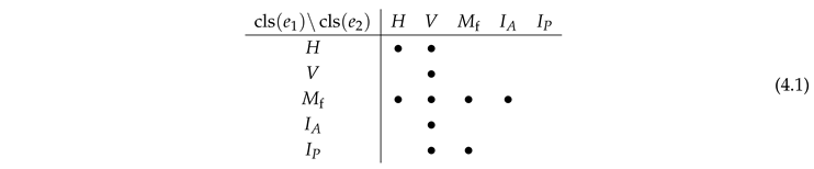
Moreover, each of the transitions
preserves the anchor:
Proof.
For a type- parent, the resulting class pairs are
Their union is exactly (4.1). Inspecting the corresponding edge pairs before passing to classes shows that every , , or pair has the same old endpoint on both sides. This proves the anchor assertion. The completeness statement preceding the lemma shows that the table is exhaustive. □
Ignoring the three self-arrows , , and , the class graph is acyclic:
Thus only an block requires more than a vertex-patch argument.
4.3.2. The Spine Relation
For a type-A or type- macro-tetrahedron K, let denote the marked edges of its two nonrefinement faces. Define the two spine relations
In canonical labels they are

Lemma 13
(Spine class transitions). Let , let , and let . With classes taken relative to , the possible ordered pairs are exactly those indicated in
For , , and , the anchor is preserved:
Proof.
Applying the classification rule in Appendix A to the two spine relations of every macrochild gives, for a type-A parent,
while for a type- parent they are
This gives the stated table. The anchor assertion follows directly from the recorded edge pairs. The parent in has type A or by item (A1), so Lemma 10 makes the enumeration exhaustive. □
4.3.3. Projection of Medial Transitions
Lemma 14
(Medial-to-spine projection). Let , and let be a different-edge horizontal transition with . Then either , or is one of the two spine relations of a tetrahedron containing the transition.
Proof.
Restrict the candidate pairs recorded in Appendix A to and apply to both entries. The resulting pairs are

The unequal pairs in the first row are precisely the two type-A spine relations, and the unequal pairs in the second row are precisely the two type- spine relations. The remaining pair in each row is equality. The completeness of the common enumeration proves the assertion for every different-edge horizontal transition. □
4.4. Proof of the Horizontal-Propagation Bound
Proof of Proposition 2.
Fix a horizontal macro-generation-q block
of event tetrahedra and write . The event tetrahedra are distinct nodes of the binary ancestry trees generated by bisection.
Low macro-generations. For a fixed initial tetrahedron, the total number of possible event tetrahedra at generations , , and is
Therefore, for ,
It remains to consider . In this range, the macro-meshes , , and consist entirely of persistent types A and , so all preceding transition tables apply.
Decomposition by edge class. If , their classes agree. If they are distinct, Lemma 12 applies. The directed class graph therefore shows that the causal chain contains at most one block of each of
Some blocks may be absent, and their order is constrained by (4.1).
Interior blocks ( and ). There is no different-edge transition or . Consequently, within either interior block all bisection edges are the same geometric edge . The fixed-edge multiplicity estimate in lem:fixededge therefore shows that each interior block has at most events.
Half-edge and spoke blocks (H and V). For an H-block, equality of consecutive edges preserves the anchor, and every different-edge transition preserves the anchor by Lemma 12. Hence all bisection edges in the block have one common anchor . Every macro-tetrahedron of containing one of those edges descends from a tetrahedron in . There are at most such macro-tetrahedra of . By Lemma 8, the block has at most
events. The same proof, using and anchor preservation, gives
The face-medial block (). Let
be the -block and put . By Lemma 14, each consecutive pair satisfies either or
as a spine relation in .
If every is equal to one fixed edge , then the carrier face of every is marked by and therefore contains . Since is conforming and , the -parent of every -tetrahedron containing contains . All relevant -macro-tetrahedra descend from the edge star . There are at most of them, so the whole -block has at most events.
Otherwise, let i be the first index for which . The prefix through is controlled by the fixed edge and therefore has at most events, as above. The nontrivial transition is a spine relation in . Since , Lemma 13, with classes relative to , shows that is of class H or V. Let be its anchor. Every later equality preserves this edge and every later nontrivial spine transition starts from an H- or V-edge; Lemma 13 shows that its target is again H or V with the same anchor a. Hence
The carrier face of is marked by , and therefore contains a. The same carrier argument shows that every event in the tail lies over the vertex star . Two macrosteps create at most tetrahedra of over that star, and Lemma 8 gives at most tail events. Consequently,
Adding the two possible interior blocks, the one medial block, and the H- and V-blocks gives
Combining this with the low-level estimate proves Proposition 2. □
5. Closure Complexity of AMP Refinement
We now derive geometric locality and the cumulative closure estimate from Proposition 2. Throughout this section, denotes the fixed constant in Proposition 2. Since it depends only on , it is not displayed as a separate argument of subsequent constants.
For nonempty sets , a point , and , write
5.1. Geometric Locality
We first record its geometric consequence.
Theorem 2
(Single-call locality). Let be an initial AMP marked mesh, let be a conformingly marked AMP descendant mesh of , let be a marking set, and let . For every , there is a causal root such that
where and is from Lemma 1.
Proof.
Let be the causal chain ending at the bisection event whose child is T. Put
By Lemma 4, . By Lemma 7,
Since T is a child of ,
Therefore
which proves (6).
For the distance estimate, the parent and child event tetrahedra intersect geometrically: the child event contains the edge whose midpoint was created by the parent event. Hence consecutive have nonempty intersection as closed sets. Also . Choosing one point in each consecutive intersection and applying the triangle inequality gives
Using Lemma 1,Proposition 2 and the fact that each integer between and occurs at most times,
Since , we have , which proves (5.2) with the stated value of . □
Remark 2.
No bound on thetotallength of a causal chain is needed. The chain may descend through arbitrarily many macro-generations. The diameters then form a geometric series. Only the number of same-scale events must be controlled. This is the central structural reduction.
5.2. A Weighted Closure Theorem
Theorem 2 associates every newly created element with a nearby marked element at a comparable level. Combined with the scale bounds in Lemma 1, this gives a uniform level-wise packing estimate. We next use a weighted double-counting argument to sum these estimates over the entire adaptive sequence and prove the closure-complexity bound.
Lemma 15
(Level-wise packing). Let denote the volume of the unit ball in . In a mesh , define the level-kR-patch around x by
Then for every , every conformingly marked AMP descendant mesh , every , and every ,
Proof.
If , then Lemma 1 implies
The interiors of the tetrahedra of a conforming mesh are disjoint, while . Comparing the sum of their volumes with the volume of the expanded ball gives
This proves the claim. □
5.2.1. Causal Witnesses
Fix an initial AMP marked mesh . A finite AMP adaptive sequence issued from is a sequence with and
Let be the disjoint union of all marking sets. Thus
For each and every , choose once and for all a witness element M (the causal root) supplied by Theorem 2, satisfying (6)–(7).
Every has a finite witness chain. Starting from its witness element, continue backward whenever the current witness element is not in . Creation times strictly decrease, so the process terminates. Thus, for some , we obtain witness elements
with , where was created by a refinement rooted at and T was created by a refinement rooted at . Hence
5.2.2. Weights
Set the constant
Fix a parameter and put
For and , define
Lemma 16
(Uniform upper weight per marked element). For every ,
Proof.
Fix M and write . If and , then and . Choose a fixed point . Because and , every such T meets . Hence Lemma 15 and (8) bound their number by , and therefore
This is the stated bound. □
Lemma 17
(Uniform lower weight). Every satisfies
Proof.
Let be a witness chain (10), put , and write . Since , . Let
Indeed, if and , then , contradicting maximality; if , then (11c) gives the same conclusion.
If , then (13) implies
and we are done because .
Assume therefore that lies outside the neighborhood of T. By (11d) and , the last witness element lies inside that neighborhood. Hence there is a largest index
Then all with lie inside the neighborhood. Also and the maximality of s imply , so all these witness elements satisfy the level condition in (12).
For closed sets one has . Applying this repeatedly along the witness chain, then using (11d), (11b), and Lemma 1, gives
For the corresponding terms are exactly . Since , multiplication by yields
This proves the stated lower bound. □
Theorem 3
(Unconditional AMP closure estimate). Every finite AMP adaptive sequence issued from an initial AMP marked mesh satisfies
Here the constant is bounded by
Proof.
Differentiating its logarithm gives the unconstrained minimizer
Since , one has , which is exactly the condition . Substitution gives the stated bound. □
Remark 3.
The DGS analysis obtains a closure estimate by relating the physical triangulation to a suitably colored triangulation in an auxiliary higher-dimensional space [8]. The present argument instead follows conformity propagation directly through the physical tetrahedra. Marked-face trees and causal chains control horizontal propagation, and the final counting argument takes place in . Consequently, neither an auxiliary dimension nor an embedding-dependent constant enters the estimate.
6. Closure Complexity of Bänsch Refinement
We next return to Bänsch’s face-based formulation. The face marking, local bisection rule, red–black transition, and proofs of termination and conformity are due to Bänsch [3]; the equivalence of the local bisection rule with is due to Arnold, Mukherjee, and Pouly [2]. The argument below first isolates the initial two-edge ambiguities and then represents every Bänsch execution, including those with history-dependent edge choices, by an AMP execution. This yields termination and a uniform closure estimate independently of how those ambiguities are resolved.
6.1. Intrinsic Face Marking
A Bänsch face marking assigns one edge
to every triangular face F. For a tetrahedron K, define its set of global refinement edges by
Bänsch’s admissibility assumptions are
- (F1)
- for every tetrahedron K;
- (F2)
- if is a face shared by two tetrahedra, then and assign the same geometric edge of F as its marked edge.
We attach each face mark intrinsically to the geometric face F, rather than separately to each tetrahedron–face incidence . Thus a shared face has a single marked edge , and item (F2) holds automatically. An intrinsic face marking is called admissible if it satisfies item (F1).
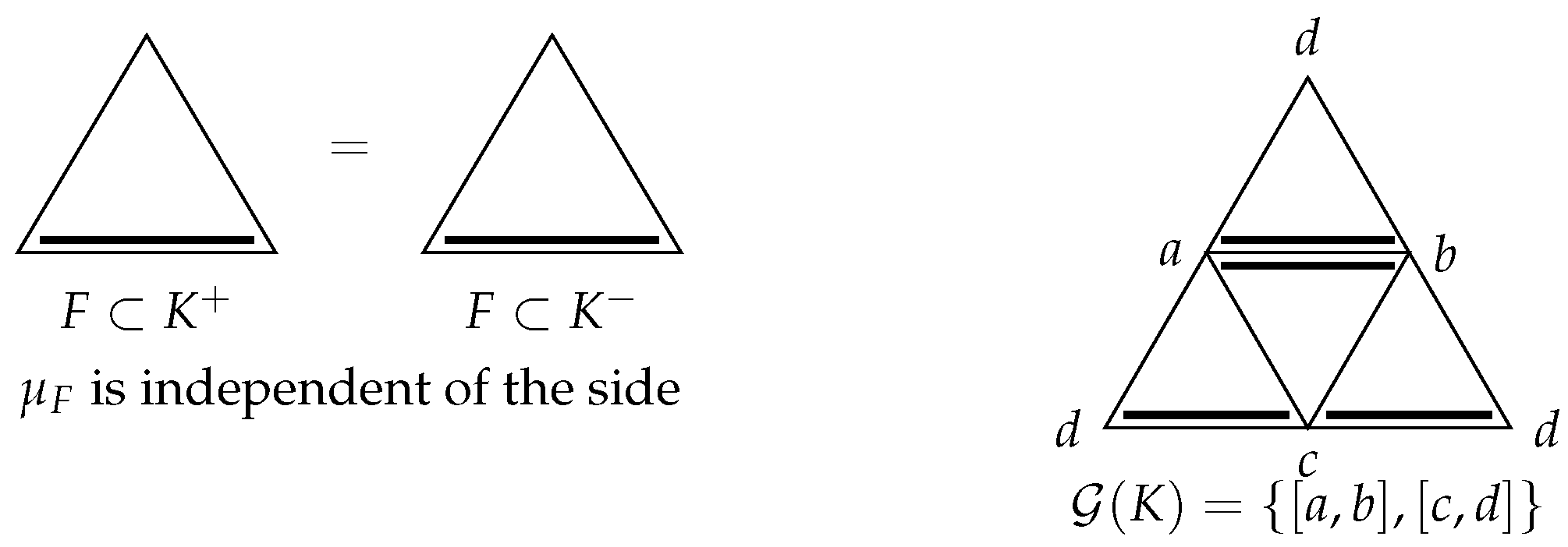
Admissible intrinsic face markings always exist. Fix a strict global order on the edges of the initial mesh and mark each face by its largest edge. The largest edge of any tetrahedron is then marked on both faces containing it and hence belongs to .
Figure 5.
Face compatibility and the two-edge ambiguity in the Bänsch marking. On the left, a shared face carries the same intrinsic mark from both incident tetrahedra. On the right, the unfolded copies show that and each mark both faces containing that edge, so both are global refinement edges; they are opposite.
Figure 5.
Face compatibility and the two-edge ambiguity in the Bänsch marking. On the left, a shared face carries the same intrinsic mark from both incident tetrahedra. On the right, the unfolded copies show that and each mark both faces containing that edge, so both are global refinement edges; they are opposite.
Lemma 18
(The two-edge alternative). An admissibly face-marked tetrahedron has either one or two global refinement edges. If it has two, they are opposite.
Proof.
A triangular face has only one mark, so two distinct global edges cannot lie in one face. Two edges of a tetrahedron fail to share a face exactly when they are opposite. The four faces incident to an opposite pair exhaust the faces of the tetrahedron, which also rules out a third global edge. □
Fix a global refinement edge , write the remaining vertices as , and set
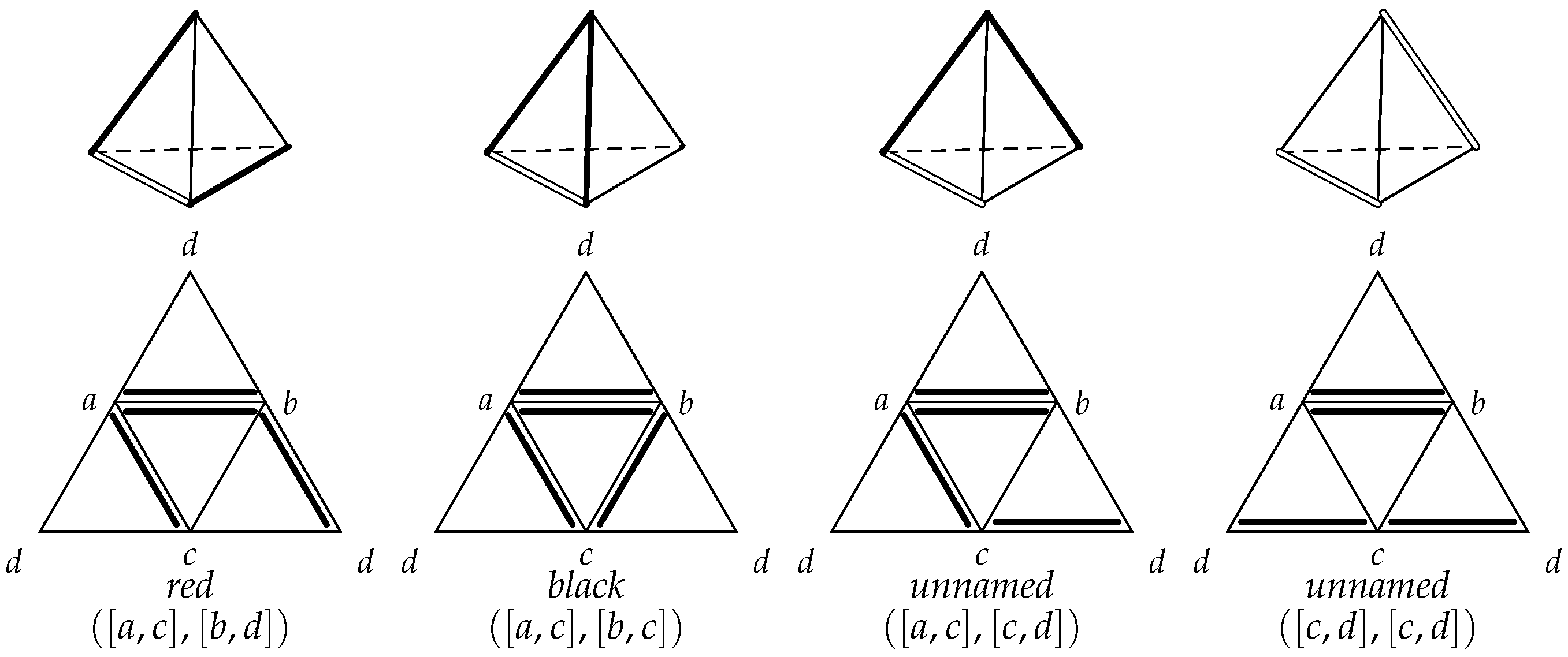
Since the two faces containing are marked by , the remaining configuration is determined by . Bänsch calls K red or black according to the following rule
In a black configuration there is therefore a unique such that . In the two remaining configurations exactly one of equals , or both do. Bänsch leaves these two configurations unnamed.
Figure 6.
The four intrinsic marking configurations relative to a selected global refinement edge , shown as marked tetrahedra (top) and unfolded face nets (bottom). The first two configurations are called red and black by Bänsch; the last two are unnamed. Thick strokes are face marks, with double strokes when both incident faces mark the same geometric edge.
Figure 6.
The four intrinsic marking configurations relative to a selected global refinement edge , shown as marked tetrahedra (top) and unfolded face nets (bottom). The first two configurations are called red and black by Bänsch; the last two are unnamed. Thick strokes are face marks, with double strokes when both incident faces mark the same geometric edge.
6.2. One Bänsch Bisection
Let K be an active tetrahedron and suppose that is the edge selected for its bisection. Write the remaining vertices as and put
Every initial tetrahedron carries the state . If K is noninitial with immediate parent T, its state is
The children and their data are determined by the following rules.
- (R1)
- An inherited face retains its mark from K.
- (R2)
- A cut face is marked by its edge opposite z; thus
- (R3)
-
If , the common new face is marked byIf , then K is black, so there is a unique with . The exceptional mark is
- (R4)
- After the face marks have been assigned, set
These are Bänsch’s local three-dimensional rules, written in intrinsic face notation.
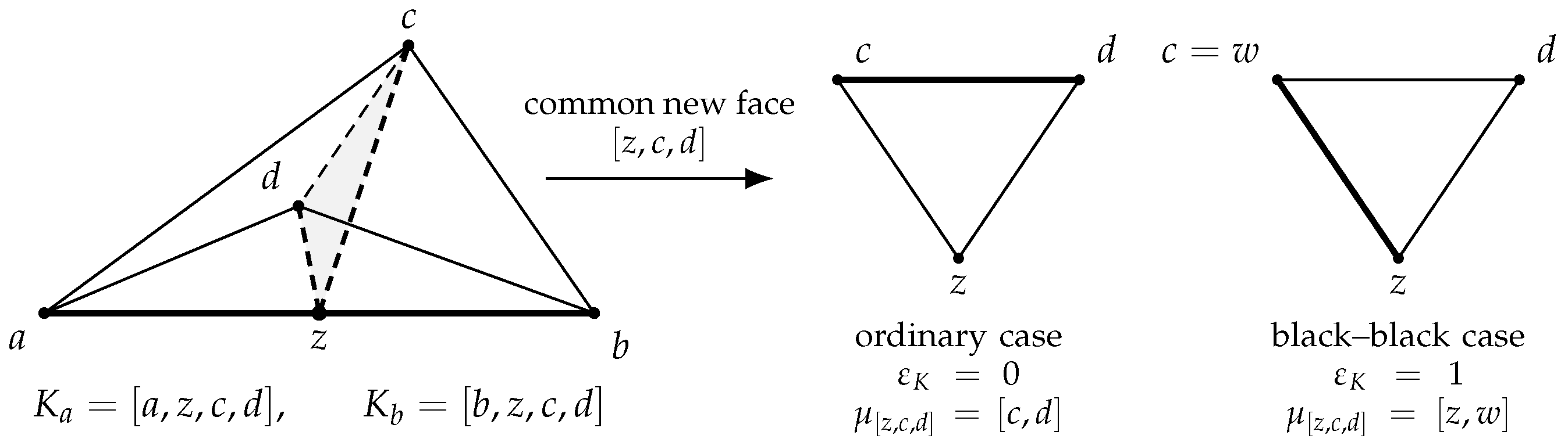
Figure 7.
One Bänsch bisection and the two possible marks of its common new face. The ordinary case uses , whereas the black–black case uses . Here ; the case is symmetric.
Figure 7.
One Bänsch bisection and the two possible marks of its common new face. The ordinary case uses , whereas the black–black case uses . Here ; the case is symmetric.
| Algorithm 4:One Bänsch bisection BänschBisectTet |
|
Input: An active tetrahedron K and a selected edge
Output: the two marked children with their states
Write and Assign the face marks and child states according to (R1)–(R4) return
|
Proposition 3
(Bänsch local structure). The two children of a Bänsch bisection have the same configuration, and each has a unique global refinement edge. Consequently, only an unbisected tetrahedron of the initial mesh can have two global refinement edges. For , write for a black tetrahedron K with . The common configuration of the two children is determined from that of the parent by
Proof.
The configuration transition is the three-dimensional case analysis in [3], sharpened for the unnamed configurations by the AMP type transition in [2].
It remains to check uniqueness. For , the four face marks are , , , and the new-face mark. If , the last mark is ; according as , , or , the unique global refinement edge of is , , or . If , then K is black, so and the new-face mark is for one ; the unique global refinement edge is then . The argument for is symmetric. Thus every child has a unique global refinement edge, which also proves the ambiguity assertion. □
6.3. Bänsch refinement
An admissible initial Bänsch marked mesh consists of a finite conforming tetrahedral mesh, an admissible intrinsic face marking, and the state on every . A current Bänsch marked mesh is the active mesh, intrinsic face marks, and states obtained from by the local rule above. In particular, its states are consistent with (R4). Moreover, every active K satisfies : an unbisected initial tetrahedron retains its nonempty set , whereas every descendant has a unique global refinement edge by prop:bansch-local. A Bänsch marked mesh is called conforming if its underlying active tetrahedral mesh is conforming.
We use the same batch terminology for Bänsch as for AMP. For either algorithm, with its initial marked mesh fixed, a finite or infinite history is a sequence arising from an execution of the algorithm, where for some , or . Here is the set of active tetrahedra bisected in batch n, and is the edge used to bisect . For AMP, ; for Bänsch, is the selected global refinement edge.
Only an initial tetrahedron K with requires a choice. It may remain active through several refinement calls; the choice is made when it is first bisected. A selection strategy assigns one edge of at that event; the choice may depend on the history preceding the current batch. We suppress this dependence below. For any active tetrahedron K selected for bisection, let denote the edge selected by in the initial two-edge case and the unique member of otherwise.
| Algorithm 5:Simultaneous Bänsch bisection BänschBisectTets |
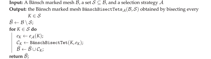 |
All edges used in a batch are determined from the fixed input marked mesh ; no child created in the batch is bisected again within that batch.
Algorithm 6 is Bänsch’s global three-dimensional refinement loop, with the deferred initial two-edge choices made explicit through .
| Algorithm 6:One Bänsch refinement call BänschRefine |
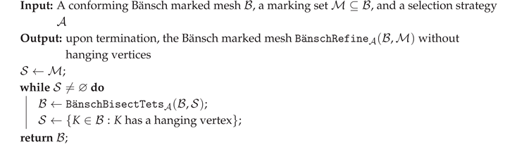 |
For the three-dimensional algorithm, Bänsch proves termination, conformity, and stability. That formulation leaves a possible two-edge choice implicit. Termination uniformly over the selection strategies above will instead follow from the deferred-resolution argument below.
6.4. Finite Resolution and AMP Correspondence
Definition 4
(Resolution space). For an admissible initial Bänsch marked mesh , let
Aresolutionis a simultaneous choice of one edge for every . The set of all resolutions is
Lemma 19
(Finite initial resolution). The resolution space is finite, with
Moreover, a resolution fixes every possible initial ambiguity, while all descendant refinement edges are unique.
Proof.
By lem:bansch-two-global, every factor in (14) consists of two opposite edges, whereas every initial tetrahedron in has a unique global refinement edge. Since the initial mesh is finite, the product is finite and has the stated cardinality. The choices in different factors are independent because they do not alter the fixed intrinsic face marks. The assertion about descendants is prop:bansch-local. □
For , select as the refinement edge of every , select the unique global refinement edge of every other initial tetrahedron, retain the intrinsic face marks, and unset all AMP flags. The resulting initial AMP marked mesh is denoted by . Thus and have the same underlying tetrahedral mesh and intrinsic face marks, while the AMP refinement edges encode the resolution of every Bänsch ambiguity.
Once the selected global edge is taken as the AMP refinement edge, the Bänsch configurations and states correspond to the AMP types and flags as follows:
| Bänsch configuration and state | AMP type | AMP flag |
| A | unset | |
| unset | ||
| set | ||
| [l]unnamed: exactly one of | ||
| equals | M | unset |
| unnamed: | O | unset |
In particular, the AMP flag is set exactly when . Under this identification, the transition graph becomes
Proposition 4
(One-step Bänsch–AMP correspondence). After a global refinement edge has been selected, one call of and one application of produce the same geometric children, face marks, and refinement edges, with corresponding Bänsch states and AMP types.
Proof.
This is the local equivalence established in [2] under the identification above. □
Theorem 4
(Deferred resolution). For every finite or infinite Bänsch history from an admissible initial Bänsch marked mesh , there exists such that is also an AMP history from .
Proof.
For each that is ever bisected in , let be the edge selected at that event; choose either edge for an ambiguous initial tetrahedron that is never bisected. This defines one fixed resolution once is fixed.
The initial geometries and face marks agree, while the Bänsch configurations and AMP types are related by the identification above. By construction, the edge selected by Bänsch at the first bisection of every ambiguous initial tetrahedron is its AMP refinement edge in . All descendants have a unique global refinement edge by prop:bansch-local; hence all later bisection edges agree automatically.
By prop:bansch-amp-onestep, the two executions produce the same children and face marks, while their Bänsch configurations and AMP types remain related as above. Hence they have the same hanging vertices, so their next conformity batches bisect the same set of geometric tetrahedra. At the beginning of each new refinement call, let the AMP execution use the same marking set as the Bänsch execution. Induction over the successive bisection batches shows that is an AMP history from . □
6.5. Uniform Bänsch Closure Complexity
A finite Bänsch adaptive process issued from an admissible initial Bänsch marked mesh specifies an integer and, at each completed step , a marking set and a selection strategy . Both choices may depend on the preceding history, and
Theorem 5
(Unconditional Bänsch closure estimate). Let be an admissible initial Bänsch marked mesh. Every finite Bänsch adaptive process issued from is well defined: all calls terminate, and the resulting sequence satisfies
where depends only on .
Proof.
Suppose that one conformity loop were infinite. Together with the preceding completed calls, its batches form an infinite Bänsch history . By the construction in the proof of thm:bansch-deferred, the same batches form an infinite AMP conformity loop from for some . The AMP execution would therefore contain infinitely many conformity batches, contradicting thm:AMPtermination. Hence every Bänsch call terminates; the same correspondence and thm:AMPtermination show that its output is conforming.
Let be the history of the resulting finite adaptive process. By thm:bansch-deferred, is also an AMP history from for some . The construction in its proof uses the same marking sets, and the two executions have the same active mesh after every batch. Applying thm:unconditional and then taking the maximum over the finite set in lem:bansch-resolution-space proves (15). Thus one may take
The proof is complete. □
In particular, thm:bansch-closure applies to every finite conforming tetrahedral mesh after a simple order-based initialization. Impose a strict global order on its geometric edges, mark each face by its maximal edge, and set for every initial tetrahedron K. Indeed, the maximal edge of K is maximal on both faces containing it and therefore belongs to , while the marking is intrinsic because the edge order is global.
7. Numerical Experiments
This section compares AMP with the DGS algorithm [8] and the AGK algorithm [1]. The Bänsch routine is not included as a separate numerical competitor. Once its ambiguous choices are fixed according to a corresponding AMP initialization, prop:bansch-amp-onestep,thm:bansch-deferred give the same history, so separate convergence curves would be redundant.
7.1. Experimental Setting
We use two three-dimensional test domains. Their initial meshes were generated with Gmsh [11]. The experiments were run in MATLAB R2024b. For each initial mesh and refinement rule, on every adaptive mesh we solve
with continuous piecewise affine finite elements, and denote the resulting Galerkin solution by . The adaptive loop uses the standard residual error indicators
where is a unit normal to F and the flux jump is constant on each interior face. At the ℓth adaptive iteration, we choose a minimal marking subset satisfying the Dörfler condition
and stop at the first iterate with at least degrees of freedom. Because an exact solution is unavailable on these domains, the figures report the residual estimator , rather than an exact energy error.
For a tetrahedron K, let
where is the inradius. We report the normalized shape parameter and the empirical closure ratio
The latter is one history-dependent observation and hence only a lower bound for a worst-case closure constant.
7.2. Fichera Corsner
The domain is the cube with the positive octant removed. We use the unstructured Gmsh mesh shown in the left panel of Figure 8. On this mesh, initialization of DGS relies on a greedy algorithm to produce a proper vertex coloring with ten colors. The numerical results are presented in Table 2 and Figure 9.
7.3. Star-Shaped Prism
The second domain is the extrusion over of a ten-vertex star whose alternating outer and inner radii are 1 and . Gmsh’s Delaunay three-dimensional algorithm provides the mesh shown in Figure 8. On this mesh, initialization of DGS relies on a greedy algorithm to produce a proper vertex coloring with eight colors. The numerical results are presented in Table 3 and Figure 10.
On the Fichera corner and star-shaped prism, all three displayed algorithms reduce the estimator with the rate , but AMP gives the smallest estimator at comparable degrees of freedom. AMP’s strict global edge ordering uses Euclidean length improves the shape-regularity of adaptive meshes. Moreover, the values of AMP are slightly smaller than DGS and AGK values, suggesting that less conforming completion was required.
7.4. Sensitivity to the Initial Vertex Numbering
We keep each physical initial mesh fixed and repeat the experiment after five independent random permutations of its vertex numbers. The permutation affects DGS and AGK through their combinatorial initializations. The coordinates and physical tetrahedra are unchanged. Trial zero uses the original numbering. All six trials use the same model problem, marking parameter, and stopping criterion as above.
For this subsection, denotes the initial refinement edge assigned to K by the method and initialization under consideration. Define its mean normalized length by
Every entry in Table 4 is the mean over the six numberings followed by the range in brackets.
This test illustrates the geometry-aware effect of AMP initialization. For every initial tetrahedron, not merely on average, AMP selects a diameter-carrying edge; hence the ratio in (16) is identically one under every permutation. DGS and AGK need not select a longest edge, and their mean ratios vary with the numbering. AMP also has an invariant final shape ratio on both meshes and completely invariant terminal data on the star prism. On the Fichera mesh, equal-length tie breaking changes some AMP histories, but its observed closure and shape statistics remain markedly more stable than those of DGS and AGK.
Appendix A. Verification of the Finite Transition Tables
By item A and lem:canonicalmacrocycle, the finite checks in Lemma 12,Lemma 13,Lemma 14 reduce, up to relabeling, to the canonical parents and . We record the resulting enumeration. Set
For , the notation denotes the marked tetrahedron specified by

The two refinement faces are marked by the refinement edge, and the flag is unset. Applying uniformly for three generations produces the following eight macrochildren of each canonical parent:
By lem:horizontalreduction, it suffices, for each macrochild , to inspect Q and its two children as possible targets T. For each such target, set
The resulting candidate arrows are, for ,
and, for ,
The first line in each display is the case . The other two relations come from its children. Each edge in braces gives a separate arrow.
It remains only to classify these arrows. In the macro-parent, set and . The carrier of has vertex set . A union of size two gives class H; a union of size three gives class V or according as one endpoint is or is not an old vertex; and a union of size four gives class or . The old endpoint is the anchor for H and V, and the marked edge of a three-vertex carrier is for .
Applying this rule to the displayed arrows gives the class and anchor assertions of Lemma 12. Applying it to the two spine relations of each macrochild gives Lemma 13 and restricting to and then applying gives Lemma 14.
References
- Alkämper, Martin; Gaspoz, Fernando; Klöfkorn, Robert. A weak compatibility condition for newest vertex bisection in any dimension. SIAM J. Sci. Comput. 2018, 40(no. 6), A3853–A3872. [Google Scholar] [CrossRef]
- Arnold, Douglas N.; Mukherjee, Arup; Pouly, Luc. Locally adapted tetrahedral meshes using bisection . SIAM J. Sci. Comput. 2000, 22(no. 2), 431–448. [Google Scholar] [CrossRef]
- Bänsch, Eberhard. Local mesh refinement in 2 and 3 dimensions . IMPACT Comput. Sci. Engrg. 1991, 3(no. 3), 181–191. [Google Scholar] [CrossRef]
- Binev, Peter; Dahmen, Wolfgang; DeVore, Ronald. Adaptive finite element methods with convergence rates . Numer. Math. 2004, 97(no. 2), 219–268. [Google Scholar] [CrossRef]
- Bonito, Andrea; Canuto, Claudio; Nochetto, Ricardo H.; Veeser, Andreas. Adaptive finite element methods . Acta Numer. 2024, 33, 163–485. [Google Scholar] [CrossRef]
- Carstensen, Carsten; Feischl, Michael; Page, Marcus; Praetorius, Dirk. Axioms of adaptivity . Comput. Math. Appl. 2014, 67(no. 6), 1195–1253. [Google Scholar] [CrossRef] [PubMed]
- Cascón, J. Manuel; Kreuzer, Christian; Nochetto, Ricardo H.; Siebert, Kunibert G. Quasi-optimal convergence rate for an adaptive finite element method . SIAM J. Numer. Anal. 2008, 46(no. 5), 2524–2550. [Google Scholar] [CrossRef]
- Diening, Lars; Gehring, Lukas; Storn, Johannes. Adaptive mesh refinement for arbitrary initial triangulations . Found. Comput. Math. 2026, 26, 1193–1218. [Google Scholar] [CrossRef]
- Dörfler, Willy. A convergent adaptive algorithm for Poisson’s equation . SIAM J. Numer. Anal. 1996, 33(no. 3), 1106–1124. [Google Scholar] [CrossRef]
- Gehring, Lukas. The constant in the theorem of Binev–Dahmen–DeVore–Stevenson and a generalisation of it . Master’s thesis, Humboldt-Universität zu Berlin, 2023. [Google Scholar]
- Geuzaine, Christophe; Remacle, Jean-François. Gmsh: A 3-D finite element mesh generator with built-in pre- and post-processing facilities . Internat. J. Numer. Methods Engrg. 2009, 79(no. 11), 1309–1331. [Google Scholar] [CrossRef]
- Karkulik, Michael; Pavlicek, David; Praetorius, Dirk. On 2D newest vertex bisection: Optimality of mesh-closure and H1-stability of L2-projection . Constr. Approx. 2013, 38(no. 2), 213–234. [Google Scholar] [CrossRef]
- Erratum to: On 2D newest vertex bisection: Optimality of mesh-closure and H1-stability of L2-projection . Constr. Approx. 2015, 42(no. 3), 349–352. [CrossRef]
- Kossaczký, Igor. A recursive approach to local mesh refinement in two and three dimensions . J. Comput. Appl. Math. 1994, 55(no. 3), 275–288. [Google Scholar] [CrossRef]
- Li, Yuwen; Yang, Zhiyuan. Closure complexity of longest-edge bisection for triangular meshes . arXiv 2026, arXiv:2609.04003. [Google Scholar]
- Liu, Anwei; Joe, Barry. On the shape of tetrahedra from bisection . Math. Comp. 1994, 63(no. 207), 141–154. [Google Scholar] [CrossRef]
- Quality local refinement of tetrahedral meshes based on bisection . SIAM J. Sci. Comput. 1995, 16(no. 6), 1269–1291. [CrossRef]
- Maubach, Joseph M. Local bisection refinement for n-simplicial grids generated by reflection . SIAM J. Sci. Comput. 1995, 16(no. 1), 210–227. [Google Scholar] [CrossRef]
- Mitchell, William F. A comparison of adaptive refinement techniques for elliptic problems . ACM Trans. Math. Softw. 1989, 15(no. 4), 326–347. [Google Scholar] [CrossRef]
- 30 years of newest vertex bisection . AIP Conf. Proc. 2016, vol. 1738, 020011. [CrossRef]
- Morin, Pedro; Nochetto, Ricardo H.; Siebert, Kunibert G. Convergence of adaptive finite element methods . SIAM Rev. 2002, 44(no. 4), 631–658. [Google Scholar] [CrossRef]
- Plaza, Ángel; Carey, Graham F. Local refinement of simplicial grids based on the skeleton . Appl. Numer. Math. 2000, 32(no. 2), 195–218. [Google Scholar] [CrossRef]
- Rivara, María-Cecilia. Algorithms for refining triangular grids suitable for adaptive and multigrid techniques . Internat. J. Numer. Methods Engrg. 1984, 20(no. 4), 745–756. [Google Scholar] [CrossRef]
- Rivara, María-Cecilia; Vénere, Marcelo J. Cost analysis of the longest-side (triangle bisection) refinement algorithms for triangulations . Engrg. Comput. 1996, 12, 224–234. [Google Scholar] [CrossRef]
- Rosenberg, Ivo G.; Stenger, Frank. A lower bound on the angles of triangles constructed by bisecting the longest side . Math. Comp. 1975, 29(no. 130), 390–395. [Google Scholar] [CrossRef]
- Sewell, Granville E. Automatic generation of triangulations for piecewise polynomial approximation . Ph.D. thesis, Purdue University, 1972. [Google Scholar]
- Stevenson, Rob. Optimality of a standard adaptive finite element method . Found. Comput. Math. 2007, 7(no. 2), 245–269. [Google Scholar] [CrossRef]
- The completion of locally refined simplicial partitions created by bisection . Math. Comp. 2008, 77(no. 261), 227–241. [CrossRef]
- Suárez, José P.; Plaza, Ángel; Carey, Graham F. The propagation problem in longest-edge refinement . Finite Elem. Anal. Des. 2005, 42(no. 2), 130–151. [Google Scholar] [CrossRef]
- Traxler, Christoph T. An algorithm for adaptive mesh refinement in n dimensions . Computing 1997, 59(no. 2), 115–137. [Google Scholar] [CrossRef]
Figure 1.
The four AMP types, shown as marked tetrahedra (top) and unfolded face nets (bottom). Thick strokes are face marks, with double strokes for an edge marked on both incident faces. The states and differ only in the Boolean flag.
Figure 1.
The four AMP types, shown as marked tetrahedra (top) and unfolded face nets (bottom). Thick strokes are face marks, with double strokes for an edge marked on both incident faces. The states and differ only in the Boolean flag.
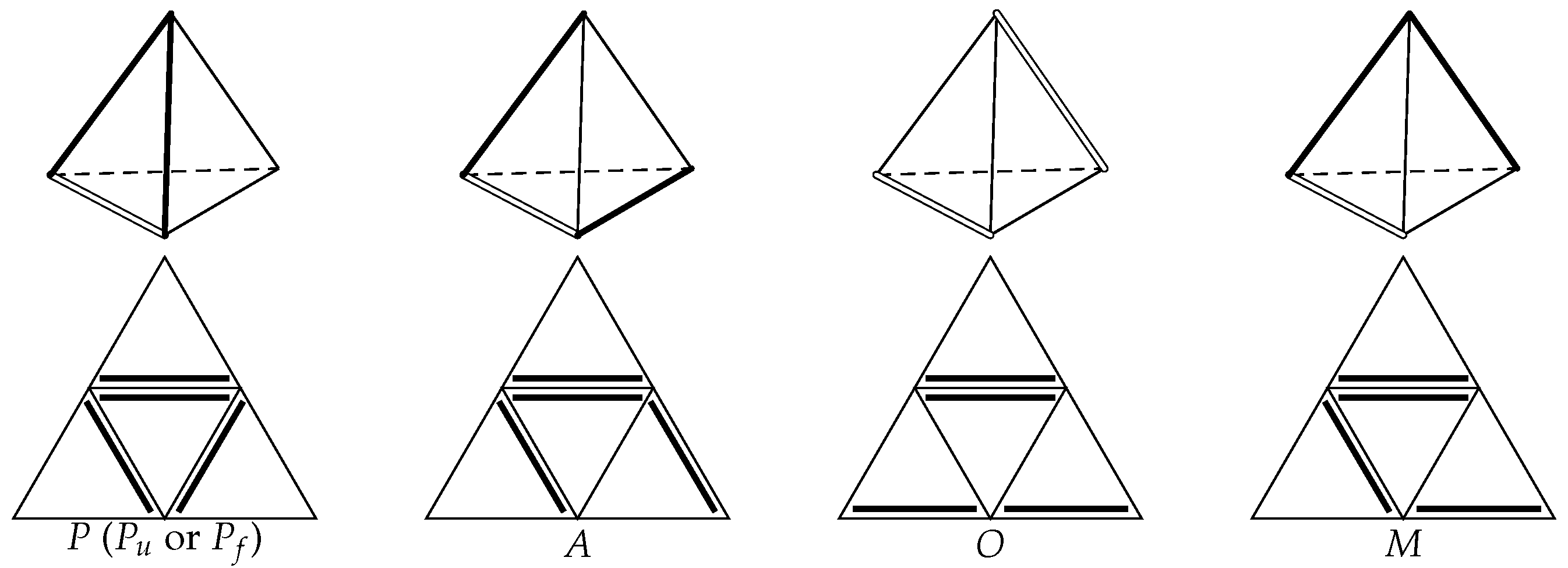
Figure 3.
The AMP type transition under one bisection. Each arrow points from the parent type to the common type of its two children.
Figure 3.
The AMP type transition under one bisection. Each arrow points from the parent type to the common type of its two children.
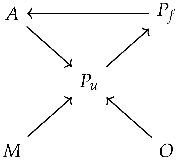
Figure 4.
A hanging vertex created on a tetrahedral interface. Initially, and share the face , and is the refinement edge of . After is bisected, its midpoint m is a vertex of the two children but not of . Dashed segments indicate edges of lying behind the shared face.
Figure 4.
A hanging vertex created on a tetrahedral interface. Initially, and share the face , and is the refinement edge of . After is bisected, its midpoint m is a vertex of the two children but not of . Dashed segments indicate edges of lying behind the shared face.
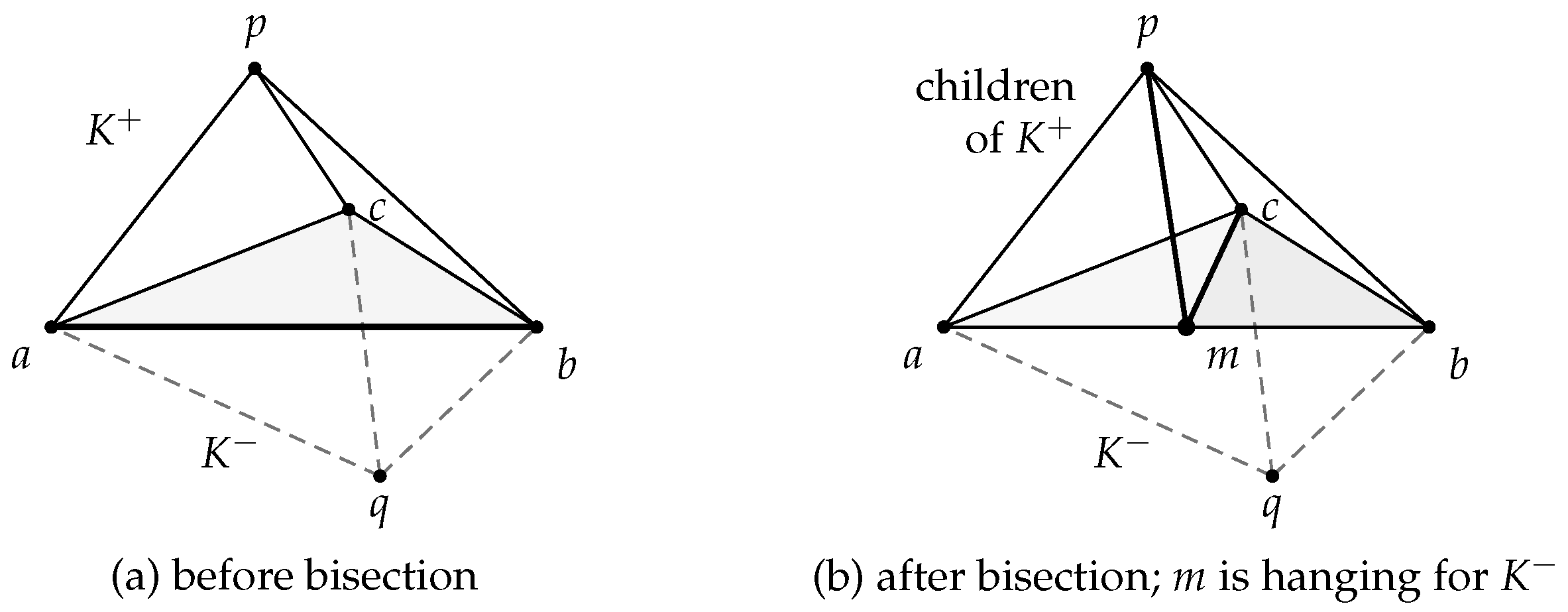
Figure 8.
The initial Gmsh-generated tetrahedral meshes. The displayed triangles are the boundary faces of the tetrahedralizations; the panel titles give the numbers of vertices and tetrahedra.
Figure 8.
The initial Gmsh-generated tetrahedral meshes. The displayed triangles are the boundary faces of the tetrahedralizations; the panel titles give the numbers of vertices and tetrahedra.
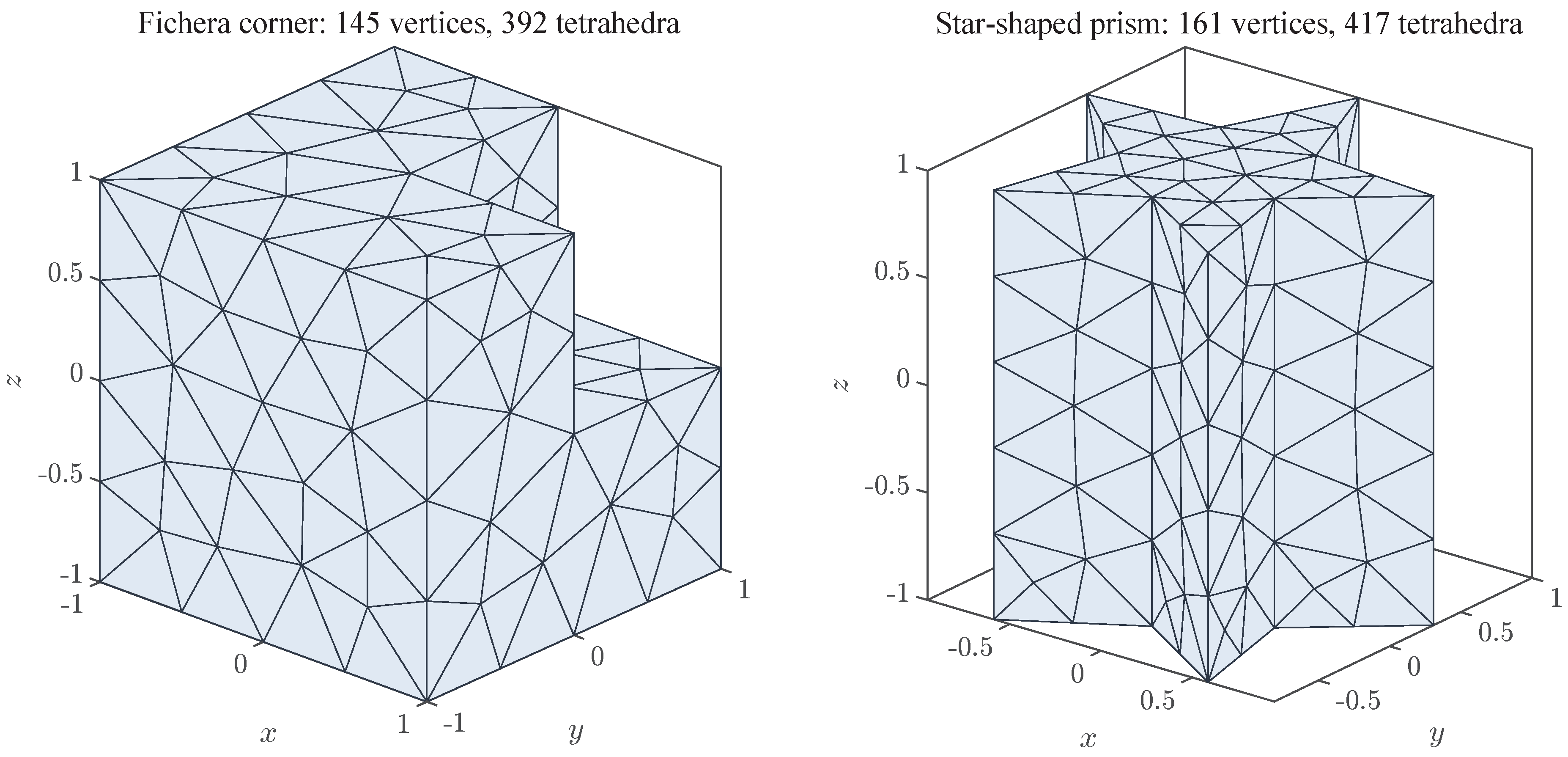
Figure 9.
Fichera corner. Left: residual estimator versus degrees of freedom; the dashed black line has reference slope . Right: normalized shape parameter along the adaptive mesh sequence.
Figure 9.
Fichera corner. Left: residual estimator versus degrees of freedom; the dashed black line has reference slope . Right: normalized shape parameter along the adaptive mesh sequence.
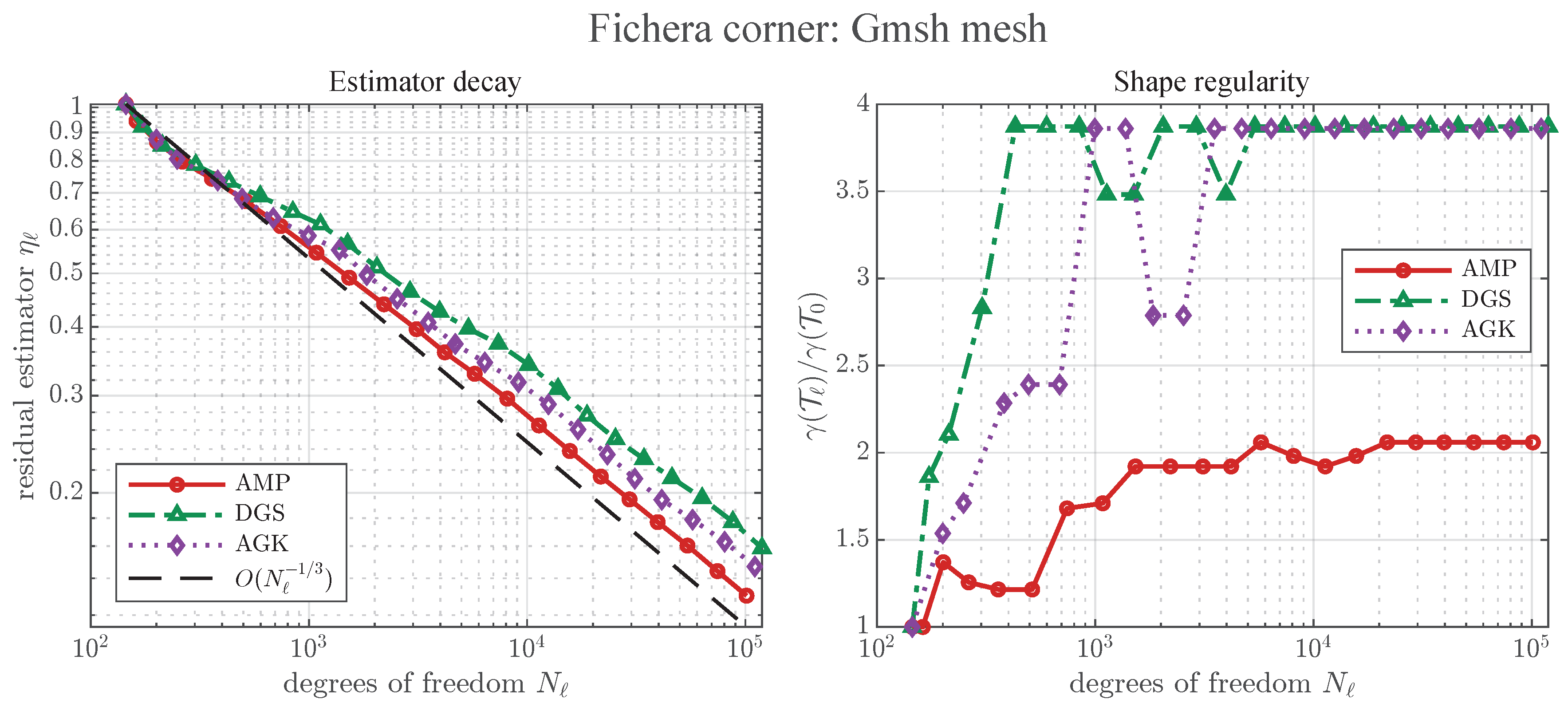
Figure 10.
Star-shaped prism. Left: residual estimator versus degrees of freedom; the dashed black line has reference slope . Right: normalized shape parameter along the adaptive mesh sequence.
Figure 10.
Star-shaped prism. Left: residual estimator versus degrees of freedom; the dashed black line has reference slope . Right: normalized shape parameter along the adaptive mesh sequence.
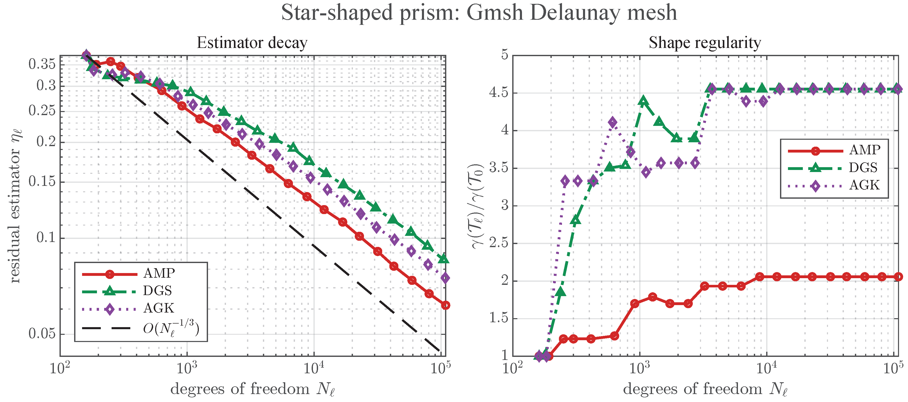

Table 1.
The rules (B1)–(B4) for a representative bisection.
| face kind | face | mark | face | mark |
| inherited | ||||
| cut | ||||
| cut | ||||
| new | ||||
| flag/type | set; | set; | ||
Table 2.
Fichera-corner results. Here L is the number of adaptive steps and is the number of degrees of freedom.
Table 2.
Fichera-corner results. Here L is the number of adaptive steps and is the number of degrees of freedom.
| Method | L | |||||
|---|---|---|---|---|---|---|
| AMP | 21 | 101206 | 524126 | 2.060 | 2.786 | |
| DGS | 22 | 119158 | 610731 | 3.872 | 2.912 | |
| AGK | 21 | 110486 | 565448 | 3.860 | 2.895 |
Table 3.
Star-prism numerical results.
| Method | L | |||||
|---|---|---|---|---|---|---|
| AMP | 21 | 108876 | 572380 | 2.058 | 2.815 | |
| DGS | 22 | 104747 | 543771 | 4.554 | 3.053 | |
| AGK | 22 | 108077 | 557750 | 4.554 | 2.985 |
Table 4.
Sensitivity to the initial vertex numbering. Each entry is the six-numbering mean followed by .
Table 4.
Sensitivity to the initial vertex numbering. Each entry is the six-numbering mean followed by .
| Fichera corner | ||||
|---|---|---|---|---|
| Method | Shape ratio | |||
| AMP | ||||
| DGS | ||||
| AGK | ||||
| Star-shaped prism | ||||
| Method | Shape ratio | |||
| AMP | ||||
| DGS | ||||
| AGK | ||||
Disclaimer/Publisher’s Note: The statements, opinions and data contained in all publications are solely those of the individual author(s) and contributor(s) and not of MDPI and/or the editor(s). MDPI and/or the editor(s) disclaim responsibility for any injury to people or property resulting from any ideas, methods, instructions or products referred to in the content. |
© 2026 by the authors. Licensee MDPI, Basel, Switzerland. This article is an open access article distributed under the terms and conditions of the Creative Commons Attribution (CC BY) license (http://creativecommons.org/licenses/by/4.0/).
Copyright: This open access article is published under a Creative Commons CC BY 4.0 license, which permit the free download, distribution, and reuse, provided that the author and preprint are cited in any reuse.