

Submitted:
04 September 2026
Posted:
04 September 2026
You are already at the latest version
Abstract
Hyper-arid agricultural soils combine low organic carbon, high calcium carbonate contents, salinity, and frequent gypsum accumulation, making rapid quantification of soil organic carbon (SOC), soil inorganic carbon (SIC), and gypsum valuable but analytically demanding. We evaluated visible–near infrared (VNIR) spectroscopy for predicting these three properties in 216 samples from 18 sites spanning two oasis management systems, three topographic positions, and six soil depths, with particular emphasis on how validation design affects apparent model accuracy. Partial least squares regression (PLSR) and random forest (RF), single- and multi-target workflows, and global versus stratified calibrations were compared using site-based GroupKFold, random KFold, and leave-one-out cross-validation (LOOCV). RF outperformed PLSR across all targets. Predictability was strongly target-specific: gypsum was predicted most reliably (R² = 0.79), SOC moderately (R² = 0.46), and SIC least reliably (R² = 0.36), with stratified SIC models often failing under site-blocked validation. KFold and LOOCV consistently yielded more optimistic estimates than GroupKFold, inflating R² by up to 0.17 for SIC. VNIR spectroscopy therefore shows strong potential for gypsum, moderate utility for SOC, but limited transferability for SIC. Validation design critically determines how soil-spectroscopy performance should be interpreted for dryland monitoring.
Keywords:
VNIR spectroscopy
; soil organic carbon
; soil inorganic carbon
; gypsum
; dryland soils
; continuum removal
; GroupKFold validation
; random forest
; multi-target modelling
; model transferability
1. Introduction (1,266 Words)
Arid and semi-arid regions cover more than 40% of the terrestrial land surface and are characterized by chronic water limitation, high evaporative demand, sparse vegetation cover, and distinctive soil biogeochemical cycles [1,2,3]. In these systems, soil carbon occurs not only as soil organic carbon (SOC), which is often constrained by low plant inputs and physical degradation, but also as soil inorganic carbon (SIC), mainly as pedogenic and lithogenic carbonates such as calcium carbonate (CaCO₃) [4,5,6,7]. Many dryland soils also accumulate gypsum (CaSO₄·2H₂O), particularly where shallow saline groundwater, evaporative concentration, topographic redistribution, or gypsiferous parent materials favour sulfate precipitation [8,9]. SOC, SIC, and gypsum are therefore central but functionally distinct constituents of dryland soils. SOC supports fertility, aggregation, nutrient cycling, and biological activity; SIC represents a major carbon pool and contributes to soil buffering; and gypsum strongly affects soil structure, water retention, hydraulic behaviour, salinity, crusting, and agricultural suitability.
The spatial distributions of SOC, SIC, and gypsum are highly heterogeneous in cultivated dryland landscapes [10,11]. Management influences organic matter inputs, irrigation, fertilization, tillage, and soil disturbance, whereas topography regulates runoff, erosion–deposition processes, groundwater depth, salt redistribution, and carbonate and gypsum accumulation. Soil depth adds a strong vertical gradient because SOC commonly decreases with depth, whereas SIC and gypsum may accumulate in subsurface horizons [12,13,14]. These interacting controls generate pronounced spatial variation over short distances, particularly in oasis and hyper-arid agricultural systems [15]. Rapid quantification of SOC, SIC, and gypsum is therefore important for soil monitoring, carbon-storage assessment, land evaluation, and agricultural management [16,17,18]. However, conventional laboratory analyses are labour-intensive, destructive, costly, and dependent on chemical reagents. Although variables such as pH, electrical conductivity, or soluble ions can be measured comparatively rapidly, specific quantification of SOC, SIC, and gypsum generally requires more demanding analytical procedures, limiting high-density monitoring in large, remote, or resource-limited dryland regions [19].
Visible–near infrared spectroscopy (VNIR; approximately 400–2500 nm) provides a rapid, non-destructive, and cost-effective alternative for estimating soil properties from diffuse reflectance spectra [20,21]. VNIR spectra integrate absorption and scattering features associated with organic matter, clay minerals, carbonates, water, gypsum, iron oxides, particle size, and surface roughness. Relevant absorptions arise mainly from overtones and combination bands of molecular vibrations, including O–H and H–O–H features associated with water, structural hydroxyl groups, and hydrated minerals; C–H, N–H, and C=O features associated with organic matter; and CO₃-related features associated with carbonates [22,23]. Gypsum has relatively diagnostic hydration-related absorption bands near 1000, 1200, 1400, 1600, 1740, 1900, and 2200 nm [12,23,24], whereas carbonate absorptions commonly occur near 2300–2350 nm [12,22,25]. By contrast, SOC signals are broader and partly indirect because organic matter affects both specific molecular absorptions and overall spectral shape, colour, and scattering behaviour [16,17]. The spectral predictability of SOC, SIC, and gypsum may therefore differ substantially, particularly where strong mineral signals overlap or mask weaker SOC features.
Previous studies have shown that VNIR spectroscopy can predict SOC across diverse soils, although performance depends strongly on SOC range, mineralogy, texture, land use, calibration design, and spectral preprocessing [17,21,26]. VNIR has also been used to estimate carbonates and gypsum in arid and semi-arid soils, although gypsum has been studied rarely. Khayamim et al. (2015) found that gypsum could be predicted more accurately than carbonates because of its stronger and more distinctive absorption features, whereas carbonate prediction was more affected by overlap with other soil constituents. That study also showed that full-spectrum PLSR could outperform continuum removal, indicating that enhancement of individual absorption features is not universally advantageous. Other proximal-sensing studies similarly demonstrate that predictions of gypsum, carbonate, salinity, SOC, and texture depend on spectral range, preprocessing, sensor type, model choice, mineralogical context, and calibration-sample distribution [27,28].
Spectral preprocessing and model choice are therefore important methodological decisions. Raw reflectance preserves full spectral shape and baseline information, whereas smoothing and scatter correction can reduce noise and effects associated with particle size, surface roughness, and illumination geometry [18]. Continuum removal can enhance diagnostic mineral bands but may also remove broadband information relevant to SOC and multivariate prediction. Likewise, partial least squares regression (PLSR) is widely used for high-dimensional, collinear spectral data [17,29], whereas random forest (RF) can capture nonlinear relationships and interactions among wavelengths [26,30]. Multi-target workflows may additionally exploit shared spectral information among SOC, SIC, and gypsum, but could perform poorly if relationships among targets vary among sites [31].
A further challenge is the strong environmental structure of dryland agricultural soils. Management, topography, and soil depth generate distinct pedological gradients, and stratified calibration may improve prediction if it reduces meaningful heterogeneity. Conversely, stratification reduces sample size and calibration range and may therefore weaken robustness and transferability [32]. Validation design is consequently critical. Random KFold cross-validation and leave-one-out cross-validation (LOOCV) can overestimate transferability when samples from the same site or related soil profiles occur in both calibration and validation subsets [17,26]. This is particularly relevant in spatially structured datasets because samples from the same site may share soil-forming history, mineralogy, management, and depth structure. GroupKFold avoids this overlap by assigning all samples from the same site to the same fold, thereby providing a stricter test of prediction at unobserved sites [33,34].
Despite substantial progress in soil VNIR spectroscopy, limited attention has been given to the simultaneous prediction of SOC, SIC, and gypsum in structured dryland agroecosystems, particularly to how validation design affects the interpretation of model performance. We therefore evaluated VNIR spectroscopy for predicting SOC, SIC, and gypsum in hyper-arid agricultural soils sampled across oasis management systems, topographic positions, and soil depths [35]. We addressed three questions: (i) how transferable are VNIR predictions of SOC, SIC, and gypsum, and how do these targets differ in predictability?; (ii) how do spectral preprocessing, model type, and single- versus multi-target workflows affect prediction performance?; and (iii) how strongly do random KFold, LOOCV, and site-based GroupKFold differ in their assessment of model transferability?
We hypothesized that prediction performance would be strongly target-specific, with gypsum showing the highest predictability because of its diagnostic hydration-related absorption features, SOC intermediate predictability because of its broader and partly indirect spectral response, and SIC weaker transferability because carbonate signals overlap with other mineral features and reflect site-specific carbonate redistribution. We further expected preprocessing and workflow effects to be target-dependent, with continuum removal benefiting properties characterized by diagnostic absorption bands, such as gypsum, while full-spectrum approaches retain useful information for broader spectral responses such as SOC. Finally, we hypothesized that GroupKFold would yield more conservative and realistic performance estimates than random KFold or LOOCV because it tests prediction at unvisited sites rather than interpolation within existing site structure.
2. Materials and Methods (2357 Words)
2.1. Study Area and Sampling Design
The study was conducted in the Djerid region of southwestern Tunisia, within the oasis landscapes of Tozeur, Deguache, and Nefta. The region is hyper-arid and lies between the hypersaline depressions of Chott El Gharsa to the north and Chott El Djerid to the south. Mean annual precipitation is approximately 80 mm, and the area is characterized by high evaporative demand, shallow saline groundwater near the chotts, and Quaternary deposits frequently enriched in gypsum. These conditions generate pronounced gradients in salinity, gypsum accumulation, carbonate redistribution, and groundwater depth.
The sampling design followed Allagui et al. (2026). Briefly, three study areas were selected within the Djerid region, with one traditional and one modern oasis system sampled in each area. Traditional oases are long-established, densely planted, structurally diverse systems with multilayered vegetation and greater reliance on organic inputs, whereas modern oases are more recently established, regularly planted date-palm systems with lower crop diversity and greater reliance on mineral fertilizers and regular irrigation (Figure S1). To capture topographic variation, one upslope, one midslope, and one downslope plot (10 × 10 m) was selected within each oasis system. Upslope plots were located farther from the Chott margin and had deeper groundwater, midslope plots represented transitional conditions, and downslope plots occurred closer to the hypersaline Chott margin, where groundwater was shallower and salinity effects were stronger.
The design therefore comprised 18 primary plots: three study areas × two oasis management systems × three topographic positions. Within each plot, soil was sampled at two positions, beneath date palms and in interspaces, at six depth intervals: 0–5, 5–10, 10–30, 30–60, 60–90, and 90–120 cm. This yielded 216 soil samples. Samples were air-dried and sieved to <2 mm before laboratory analyses and VNIR measurements.
2.2. Laboratory Analyses
Soil total carbon (STC), soil organic carbon (SOC), and soil inorganic carbon (SIC) were determined as described in Allagui et al. (2026) [35]. Briefly, soil samples were oven-dried at 105 °C, homogenized, coarsely ground with a mortar and pestle, and subsequently finely ground in a ball mill at 25 Hz for 5 min (Retsch MM200, Haan, Germany). STC was measured on untreated finely ground soil. SOC was measured on a separate aliquot after carbonate removal by pretreatment with 2 M HCl for 60 min, followed by drying at 105 °C. Carbon concentrations were determined using an elemental analyzer (EA-Isolink) coupled via a ConFlo IV interface to a Delta V Advantage isotope ratio mass spectrometer (Thermo Scientific, Vienna, Austria). SIC was calculated by difference:
SIC = STC − SOC
where SIC is soil inorganic carbon, STC is soil total carbon, and SOC is soil organic carbon.
Gypsum (CaSO₄·2H₂O) was quantified using a dissolution–ion chromatography assay, following Allagui et al. (2026). Briefly, 50 mg of finely ground, oven-dried soil was extracted with 25 mL ultrapure water for 18 h, using an extraction ratio sufficient to dissolve the gypsum present. Extracts were centrifuged at 10,000 rpm for 10 min, and dissolved Ca²⁺ and SO₄²⁻ were measured by high-performance ion chromatography using a Dionex ICS5000 system (Thermo Scientific, Vienna, Austria). Cations were separated on a Dionex IonPac CS16 column and anions on a Dionex IonPac AS11-HC column, using CERS 500 and AERS 500 suppressors, respectively. Because dissolution of CaSO₄·2H₂O releases Ca²⁺ and SO₄²⁻ in a 1:1 molar ratio, gypsum content was calculated from the lower molar amount of the two ions, assuming the limiting ion represented the amount of dissolved gypsum.
Soil pH was measured electrometrically in a 1:2.5 soil-to-water suspension using an inoLab pH 7110 pH meter. Electrical conductivity (EC) was measured in a 1:5 soil-to-water extract using a Consort C862 conductivity meter. Soil texture was determined using the simplified sedimentation method of Kettler et al. (2001)[36], in which sand is separated by sieving and the remaining fine fraction is partitioned into silt and clay according to particle settling times in water. These supporting variables were used to characterize the dataset and interpret spectral model behaviour but were not included as predictors in the VNIR models.
2.3. VNIR Spectral Acquisition
Diffuse reflectance spectra were acquired in a dark room using an ASD FieldSpec® 3 spectroradiometer (Analytical Ltd., London, UK) covering 350–2500 nm, with spectral sampling intervals of 1.4 nm from 350–1000 nm and 2 nm from 1000–2500 nm. Soil samples were placed in 5-cm diameter Petri dishes to a depth of approximately 1 cm and levelled before measurement. For each sample, four replicate spectra were recorded with a standard contact probe equipped with an internal light source (colour temperature ca. 3400 K), rotating the dish by 90° between scans to reduce effects of particle orientation and surface heterogeneity. Each replicate spectrum was averaged from 30 internal scans. A Spectralon® white reference panel (Labsphere Inc., North Sutton, NH, USA) was measured before sample acquisition and approximately every 15–20 min thereafter. The four replicate spectra per sample were averaged, and noisy edge regions were removed before modelling. The final raw spectra covered 400–2500 nm.
2.4. Spectral Preprocessing
The analytical workflow comprising spectral scenarios, calibration paths, model families, validation schemes, and performance metrics is summarized in Figure 1. Three spectral predictor matrices were evaluated, and their mean spectra are shown in Figure S5. First, raw reflectance spectra (RAW) were retained after wavelength trimming. Second, spectra were processed using Savitzky–Golay smoothing followed by multiplicative scatter correction (RAW+SG+MSC) to reduce high-frequency noise and additive and multiplicative scatter effects. Third, continuum removal (CR) was applied to enhance absorption features relative to the spectral continuum. For each spectrum, an upper convex hull was fitted to define the continuum, and continuum-removed reflectance was calculated as:
where RCR(λ) is the continuum-removed reflectance at wavelength λ, R(λ) the measured reflectance, and C(λ) the continuum reflectance at wavelength λ. RAW, RAW+SG+MSC, and CR spectra were compared under GroupKFold validation for SOC, SIC, and gypsum. The main model interpretation was based on the preprocessing–model combinations retained from this validation-aware comparison, while the full preprocessing comparison is reported in the Supplementary Material.
The dataset comprised 216 dryland soil samples from 18 plots, measured at 400–2500 nm (2101 wavelength variables). Three spectral scenarios were evaluated: untransformed reflectance (RAW), Savitzky–Golay first-derivative preprocessing with multiplicative scatter correction (RAW+SG+MSC), and continuum removal (CR). Models were fitted using three calibration paths: Path A, global; Path B1, management-stratified; and Path B2, topography-stratified. Partial least squares regression (PLSR) was evaluated for Path A, whereas random forest (RF) was evaluated for all paths; both single- and multi-target workflows were tested. Model performance was assessed using plot-based GroupKFold cross-validation (six folds, plots kept intact; primary validation), random five-fold KFold, and leave-one-out cross-validation (LOOCV). Held-out predictions were pooled across folds before calculating performance metrics, and ΔR² quantifies the optimism of non-grouped validation relative to GroupKFold. Green shading and checkmarks indicate the CR–RF–GroupKFold configuration retained for the main model interpretation; additional model and preprocessing combinations are reported in the Supplementary Material.
2.5. Modelling Design
VNIR spectra were used as the only predictor variables. Management, topography, and soil depth were not included as covariates; instead, management and topography defined stratified calibration subsets. Prediction performance therefore reflected spectral information rather than direct inclusion of environmental class labels.
Three modelling paths were evaluated. Path A comprised a global calibration using all 216 samples. Path B1 comprised separate management-stratified calibrations for modern and traditional oasis systems (108 samples each), and Path B2 separate topography-stratified calibrations for upslope, midslope, and downslope positions (72 samples each). The stratified paths tested whether reducing environmental heterogeneity improved prediction despite the smaller calibration subsets.
Two algorithms were compared. Partial least squares regression (PLSR) was used as a standard linear method for high-dimensional, collinear spectral data; it reduces the spectral predictor matrix to a smaller set of latent variables that maximize covariance with the response. Random forest (RF) was used to capture nonlinear relationships and interactions among wavelengths by combining predictions from multiple regression trees fitted to bootstrap samples. PLSR was evaluated only for the global path, while RF was applied to all three paths.
Single-target and multi-target workflows were compared. In the single-target workflow, SOC, SIC, and gypsum were modelled separately. In the multi-target workflow, the three properties were modelled jointly as a 216 × 3 response matrix. For PLSR, this corresponded to a PLS2 model with shared latent variables [29]; for RF, a native multi-output forest predicted all three responses using shared tree structures [37,38]. Because the multi-output RF splitting criterion combines squared errors across responses expressed in their original mass-percent units, the target with the largest numerical variance gypsum in this dataset can exert greater influence on split selection than SOC or SIC.
The multi-target workflow was used to test whether shared spectral information among SOC, SIC, and gypsum improved prediction. Such information may arise because mineral constituents can influence or mask overlapping spectral regions, but joint modelling may also reduce transferability if relationships among targets differ among plots. RF was therefore used for both global and stratified paths, allowing the effects of management and topographic stratification to be evaluated without introducing additional model-family differences.
2.6. Validation Strategy
Three validation strategies were compared. Plot-based GroupKFold was used as the primary validation because it tests transferability to held-out plots while respecting the hierarchical structure of the dataset. The grouping variable was plot, with 18 plot levels, and all samples from a given plot were assigned to the same fold so that no plot contributed simultaneously to calibration and validation. Six folds were used for GroupKFold, five shuffled folds for random KFold (random_state = 42), and one held-out sample per fold for leave-one-out cross-validation (LOOCV). Blocking cross-validation according to the dependence structure of the data follows recommendations for spatially and hierarchically structured datasets [34].
Random KFold and LOOCV were used as supplementary benchmarks of internal predictive performance. In random KFold, individual samples were randomly assigned to five folds, allowing samples from the same plot to occur in both calibration and validation sets. In LOOCV, each sample was held out once while all remaining samples were used for calibration. Both approaches can therefore yield optimistic performance estimates when samples within plots are correlated.
Under GroupKFold, the global path used 180 training and 36 validation samples per fold. Management-stratified models contained nine plots per management class; consequently, individual folds contained one or two held-out plots, corresponding to 84–96 training and 12–24 validation samples. Topography-stratified models contained six plots per topographic class and therefore used 60 training and 12 validation samples per fold. For all models and validation schemes, held-out predictions were pooled across folds, and each performance metric was calculated once from the pooled predictions rather than averaged across folds. This also avoids undefined fold-level R² for LOOCV and unstable averaging across small validation folds.
2.7. Performance Metrics
Model performance was evaluated using the coefficient of determination (R²), root mean square error (RMSE), mean absolute error (MAE), bias, ratio of performance to deviation (RPD), and Lin’s concordance correlation coefficient (CCC). All metrics were calculated from pooled held-out predictions for each validation scheme.
For n observations, with observed values yᵢ, predicted values ŷᵢ, mean observed value ȳ and mean predicted value ӯ, R² was calculated as:
Negative R² values were retained and indicate performance worse than predicting the mean observed value. To quantify optimism from non-grouped validation, ΔR² was calculated as:
Positive ΔR² therefore indicates higher apparent performance under non-grouped than plot-based GroupKFold validation.
RMSE, MAE, and bias were calculated as:
Positive bias indicates overprediction and negative bias underprediction.
RPD was calculated as:
where SD(y) is the standard deviation of the pooled observed values.
Lin’s CCC was calculated as:
where ρ is the Pearson correlation coefficient between observed and predicted values, σy and σŷ are their standard deviations, and ȳ and ӯ their means. CCC evaluates both precision and agreement with the 1:1 relationship.
2.8. Computational Implementation and Software
All spectral preprocessing, model fitting, validation, performance evaluation, wavelength-importance analysis, and figure/table generation were implemented in Python 3.14.0 using custom scripts. Data handling used pandas 3.0.2 [39], numerical operations NumPy 2.4.4 (Harris et al., 2020), signal processing SciPy 1.17.1 [40], and chemometric and machine-learning workflows scikit-learn 1.8.0 [41]. Figures were generated with Matplotlib 3.10.8 [42] and seaborn 0.13.2 [43], and SHAP 0.51.0 was used for post hoc interpretation of RF models and wavelength importance [44]. Random forest fitting and random KFold partitioning used a fixed random seed (random_state = 42) to ensure reproducibility.
Savitzky–Golay first-derivative preprocessing was implemented with scipy.signal.savgol_filter using a window length of 11 wavelength points, polynomial order 3, and derivative order 1 [45]. Multiplicative scatter correction was performed within each calibration fold by regressing individual spectra against the mean calibration spectrum and correcting additive and multiplicative scatter effects. Continuum removal was implemented by fitting an upper convex hull to each reflectance spectrum and dividing measured reflectance by the corresponding continuum reflectance.
For PLSR, the number of latent variables was selected independently within each outer calibration fold using inner five-fold shuffled cross-validation (random_state = 42) over candidate values from 1 to min(25, n_train − 1, n_features − 1), minimizing RMSE using calibration data only. The same procedure was applied to single-target and multi-target (PLS2) models. RF models were fitted with 260 trees for GroupKFold and KFold and 120 trees for LOOCV, using squared-error splitting, unrestricted tree depth, min_samples_leaf = 1, and max_features = "sqrt" [30]. Multi-target RF models used the native multi-output implementation in scikit-learn on the untransformed response matrix in mass-percent units, whereas single-target RF models fitted one independent forest per target.
3. Results (2142 Words Incl. Captions and Tables)
3.1. Soil Property Variability and Spectral Structure
The dataset showed substantial variation in SOC, SIC, and gypsum (Table S4). SOC concentrations were generally low, ranging from 0.04 to 4.20% (mean 0.74%), whereas SIC varied over a narrower range of 0.21–3.80% (mean 1.65%). Gypsum showed the greatest variability and strong positive skew, ranging from 0 to 69.83% (mean 5.95%). Soils were predominantly sandy (50–95%; mean 77.4%), with lower silt (1–25%; mean 9.1%) and clay contents (2–38%; mean 13.2%). Soil pH ranged from 7.3 to 8.6 (mean 7.9), and EC from 0.31 to 3.57 dS m⁻¹ (mean 1.50).
SOC, SIC, and gypsum showed contrasting distributions across topography, depth, and management (Figure 2 and Figure S2). SOC declined strongly with depth across most topography–management combinations, with highest concentrations in surface soils and markedly lower values below 30 cm. SIC showed substantial overlap among groups, with only a modest tendency towards higher concentrations downslope. Gypsum showed the strongest environmental differentiation, with high concentrations occurring mainly in traditional oases, particularly at downslope positions and in the 60–90 and 90–120 cm depth intervals. Overall, depth most strongly structured SOC, whereas management and topographic position were more evident for gypsum; SIC showed comparatively weak categorical separation.
Principal component analysis of the VNIR spectra showed partial but no distinct separation among management systems or topographic positions, while soil depth formed a secondary spectral gradient (Figure 3). Correlations among SOC, SIC, gypsum, EC, pH, and texture variables were generally moderate rather than redundant (Figure S3).
Panels show the three target soil properties by topographic position, with soil depth on the x-axis and oasis management distinguished within each depth class (Modern, blue; Traditional, green). Row annotations report P values for the main effects of soil depth, topography, and oasis management from linear mixed-effects models accounting for the hierarchical sampling design and repeated depth structure. Gypsum is shown on a symmetrical logarithmic y-axis to accommodate its strongly right-skewed distribution and zero values. Abbreviations: SOC, soil organic carbon; SIC, soil inorganic carbon.
Principal component analysis was performed on the preprocessed VNIR spectral matrix. a, Samples coloured by topographic position and shaped by oasis management type. b, The same ordination coloured by soil depth. The ordination shows partial spectral structuring by environmental factors but no distinct separation among management systems or topographic positions. Abbreviations: VNIR, visible–near infrared; PC, principal component.
3.2. Effects of Spectral Preprocessing and Prediction Workflow
The three spectral variants raw reflectance (RAW), continuum removal (CR), and Savitzky–Golay first-derivative preprocessing with multiplicative scatter correction (RAW+SG+MSC)—showed distinct mean spectral patterns (Figure S5).
Preprocessing effects differed strongly among target properties (Table S1). Gypsum was predicted reliably across all three spectral variants. The highest GroupKFold performance was obtained with RAW multi-target PLSR (R² = 0.81, RMSE = 5.48%, RPD = 2.28), while CR-based RF models performed nearly as well (R² = 0.79 for both single- and multi-target workflows); RF performance with RAW and RAW+SG+MSC was only slightly lower (R² = 0.77–0.78). Thus, gypsum prediction was comparatively robust to preprocessing and model choice.
SOC benefited more clearly from preprocessing. RAW spectra yielded weak to moderate performance, with PLSR reaching R² = 0.31–0.32 and RF R² = 0.12–0.22. Performance increased with CR and especially RAW+SG+MSC, with the highest SOC prediction obtained by multi-target RF using RAW+SG+MSC (R² = 0.48, RMSE = 0.52%, RPD = 1.38). CR-based multi-target RF was only slightly weaker (R² = 0.46), indicating that both preprocessing approaches substantially improved SOC prediction relative to RAW RF models.
SIC was the least predictable and most preprocessing-sensitive target. RF models based on RAW spectra performed poorly (R² < 0), whereas RAW+SG+MSC increased RF performance to R² = 0.31–0.32. The best SIC result was obtained with CR-based multi-target RF (R² = 0.36, RMSE = 0.58%, RPD = 1.25), compared with R² = 0.30 for single-target RF. Thus, CR provided the strongest transferable SIC prediction, although overall performance remained modest.
Multi-target modelling did not provide a consistent advantage across targets. It modestly improved the best RF predictions of SOC and SIC but had essentially no effect on gypsum RF performance (Table S1). Overall, preprocessing and workflow effects were therefore target-specific rather than universally beneficial.
3.3. Global Model Performance and Validation Effects
For the global modelling path using CR spectra, RF outperformed PLSR across all three target properties under plot-based GroupKFold validation (Table 1). RF performance was highest for gypsum (R² = 0.79), intermediate for SOC (R² = 0.46), and weakest for SIC (R² = 0.36), whereas PLSR produced negative R² values for SIC. The RF advantage persisted despite optimization of the number of PLSR latent variables by inner cross-validation.
Validation strategy strongly affected apparent model performance (Figure 4; Table S3). For the best global RF models, R² increased from 0.46 under GroupKFold to 0.53–0.54 under KFold and LOOCV for SOC, and from 0.36 to 0.48–0.53 for SIC. Gypsum showed the same pattern but a smaller relative effect, increasing from R² = 0.79 to 0.88. Other performance metrics showed corresponding improvements under non-grouped validation (Table S3), confirming that random KFold and LOOCV yielded systematically more optimistic estimates than plot-based GroupKFold.
The validation effect was particularly pronounced for SIC. For the global multi-target RF model, moving from GroupKFold to LOOCV increased R² from 0.36 to 0.53, reduced RMSE from 0.58 to 0.50%, and increased CCC from 0.54 to 0.67 and RPD from 1.25 to 1.46 (Table S3). A similar discrepancy occurred in topography-stratified SIC models: KFold and LOOCV yielded positive R² values, whereas all three topographic strata showed negative R² under GroupKFold (Figure S4; Table 2). Thus, within-plot predictive structure did not translate into reliable prediction of held-out plots.
3.4. Effects of Management and Topography Stratification
Stratification effects differed strongly among target properties (Table 2). Gypsum showed the most robust performance. Management-stratified models reached R² = 0.79 in modern and 0.82 in traditional oases under both single- and multi-target workflows. Topography-stratified models also remained predictive, with R² = 0.72 upslope, 0.66 downslope, and 0.50–0.52 midslope. Thus, gypsum prediction remained transferable across held-out plots under both stratification approaches, with the strongest performance under management stratification.
SOC performance remained positive across all strata but varied among subsets. The highest R² was obtained for midslope soils using multi-target RF (R² = 0.55, RMSE = 0.39%, RPD = 1.50), closely followed by the traditional oasis subset using single-target RF (R² = 0.55, RMSE = 0.48%, RPD = 1.49). Modern, upslope, and downslope models showed lower but consistently positive performance (Table 2).
SIC showed the opposite response. Its best plot-based GroupKFold performance was obtained with the global multi-target RF model (R² = 0.36; Table 1), whereas stratification generally reduced predictive performance. Management-stratified SIC remained positive in modern oases (R² = 0.31) but was negative in traditional oases (R² = −0.25). All topography-stratified SIC models had negative R² under GroupKFold (−0.09 to −0.40), despite positive performance under KFold and LOOCV (Figure S4; Table S2). Thus, stratification improved or maintained prediction only for selected target–stratum combinations: it was most effective for gypsum, beneficial for SOC in specific subsets, but did not improve transferable SIC prediction.
3.5. Model Interpretation Using SHAP
SHAP analysis was used to identify wavelengths contributing most strongly to RF predictions. Mean absolute SHAP values quantify the overall importance of individual wavelengths across samples.
Wavelength-importance patterns differed among target properties but showed substantial overlap between SIC and gypsum (Figure 5). For SOC, the five highest-ranked wavelengths in the CR model clustered at 1842–1848 nm. SIC importance was concentrated mainly at 2314–2327 nm, whereas gypsum also showed strong contributions around 2324–2328 nm, together with additional wavelengths near 1926 and 2390 nm. Thus, SOC relied on a distinct spectral region, while SIC and gypsum partly shared wavelength regions around 2320–2330 nm.
The overlap between SIC and gypsum is consistent with their partly overlapping mineral spectral signatures and may contribute to the lower transferability of SIC relative to gypsum. However, SHAP identifies wavelengths used by the RF models rather than isolated chemical absorption mechanisms, and importance at correlated wavelengths should therefore not be interpreted as direct evidence of specific molecular or mineral features.
4. Discussion (1325 Words)
4.1. Validation Design Determines the Interpretation of Model Performance
A central result of this study is that model performance depended strongly on validation strategy. Random KFold and LOOCV consistently yielded higher apparent predictability than plot-based GroupKFold, with the largest discrepancy for SIC. For the global multi-target RF model, SIC R² increased from 0.36 under GroupKFold to 0.48 under KFold and 0.53 under LOOCV, accompanied by lower RMSE and higher CCC and RPD. Thus, non-grouped validation improved not only R² but the overall apparent accuracy and agreement of the model.
This difference is methodologically important because random KFold and LOOCV allow samples from the same plot to occur in both calibration and validation subsets. Such samples may share parent material, hydrological history, management, salinity, depth structure, and mineralogical background, thereby increasing similarity between training and validation data. Plot-based GroupKFold avoids this overlap by withholding entire plots and therefore provides a stricter test of transferability beyond the calibration plots [34,46]. Reliance only on KFold or LOOCV would consequently have overstated model transferability, particularly for SIC. These results support our hypothesis that grouped validation provides more conservative and realistic estimates of predictive performance in hierarchically structured dryland datasets.
4.2. Target-Specific Predictability of SOC, SIC, and Gypsum
Prediction performance was strongly target-specific, following the order gypsum > SOC > SIC. Gypsum was the most predictable property, likely because of its diagnostic hydration-related absorption features and the wide concentration range represented in the dataset. RF models maintained high performance under plot-based GroupKFold, particularly after management stratification. This agrees with previous work showing more accurate VNIR prediction of gypsum than carbonates in arid and semi-arid soils, attributed to the stronger and more distinctive spectral features of gypsum [12]. Our results extend these findings to a stricter plot-blocked validation framework.
SOC showed moderate predictability, consistent with the low SOC concentrations (0.04–4.20%) and strong mineral background of these sandy, alkaline, hyper-arid soils. At low SOC contents, organic-matter-related VNIR signals may be weak relative to variation associated with carbonates, gypsum, salinity, and texture. Higher SOC prediction performance has been reported under other calibration conditions. For example, Marques et al. (2020) [47] obtained R² = 0.74 in gypsiferous agricultural soils using PLSR, while broader studies show strong dependence of SOC prediction on concentration range, mineralogy, preprocessing, and validation design [16,21,48]. The moderate performance observed here therefore likely reflects both the low SOC range and the more stringent plot-based validation.
SIC was the least transferable target. SIC comprises lithogenic and pedogenic carbonate pools influenced by parent material, hydrology, pH, evaporation, irrigation, dissolution–precipitation processes, and biological CO₂ inputs. Its relatively narrow concentration range (0.21–3.80%) and weak separation among management and topographic groups further constrained calibration. In addition, carbonate absorptions in the VNIR/SWIR region can overlap with clay-mineral and gypsum-related features. Previous studies similarly indicate lower robustness of carbonate than gypsum prediction and mineralogical interference around the 2300–2350 nm carbonate region [12,22,49]. Our results further show that moderate SIC performance under random validation does not necessarily translate into reliable prediction across held-out plots.
4.3. Preprocessing and Multi-Target Workflows Revealed Target-Specific Spectral Information
No single preprocessing strategy was optimal across all targets. Gypsum prediction was robust with RAW, RAW+SG+MSC, and CR spectra, with the strongest RF performance obtained after continuum removal. Nevertheless, RAW and RAW+SG+MSC retained substantial predictive information, consistent with previous studies showing that full-spectrum approaches can perform as well as or better than feature-specific continuum removal for gypsum and carbonates [12,49].
SOC and SIC were more sensitive to preprocessing. For SOC, RF performance improved markedly from RAW spectra to CR and RAW+SG+MSC, with the latter giving the highest performance. SIC showed a similar improvement relative to RAW, but its highest RF performance was obtained with CR, followed closely by RAW+SG+MSC. These results indicate that both absorption enhancement and broader preprocessing of spectral structure can improve prediction, with their relative benefits depending on the target property.
Multi-target workflows likewise provided target-specific rather than uniform benefits. Joint prediction slightly improved global RF performance for SOC and SIC but had little effect on gypsum. This suggests that shared spectral information among the three properties can be useful, although relationships among targets may not remain stable across plots. The SHAP analysis supports partial spectral overlap: SOC importance was concentrated around 1842–1848 nm, whereas SIC and gypsum shared important wavelengths in the 2320–2330 nm region. Gypsum additionally showed contributions around 1926 and 2390 nm, consistent with hydration-related spectral features [16,18,23,24,50]. This broader spectral information may partly explain the greater robustness of gypsum prediction, whereas the overlap between SIC and gypsum may contribute to weaker SIC transferability. However, SHAP identifies predictive wavelength associations rather than isolated chemical absorption mechanisms.
4.4. Stratification Improves Prediction only When it Matches Soil Structure
Environmental stratification did not universally improve prediction. Management stratification maintained strong gypsum performance and supported SOC prediction, whereas topographic stratification did not improve transferable SIC prediction. Stratification can therefore be beneficial when it reduces meaningful heterogeneity, but smaller calibration subsets may also reduce robustness [1,21,51].
The soil-property distributions partly explain these contrasting responses. SOC was structured mainly by depth, whereas gypsum showed clear management-related differentiation, with high concentrations concentrated in traditional oases and in deeper, downslope soils. This likely contributed to the strong performance of management-stratified gypsum models.
By contrast, SIC was only weakly separated among management and topographic classes. The global multi-target RF model therefore outperformed the stratified models under plot-based GroupKFold, while all topography-stratified SIC models produced negative R². Their positive performance under KFold and LOOCV suggests that topography captured local structure that did not transfer to held-out plots. Reduced calibration size may have further limited SIC model stability because of its narrow concentration range and weak group separation [34,52].
4.5. Implications for VNIR Monitoring of Dryland Soil Carbon and Gypsum
VNIR spectroscopy showed strongly target-dependent potential for dryland soil monitoring. Gypsum was predicted with high accuracy and good transferability, making it the most promising target for rapid screening in these hyper-arid oasis soils. SOC showed moderate predictability and may be useful for identifying broad spatial gradients, although low SOC concentrations and strong mineral-background effects limit precision. SIC remained the least transferable target: global RF models achieved only moderate performance, and stratification did not overcome this limitation.
Our gypsum results are consistent with the generally strong VNIR predictability reported for gypsum in arid soils, whereas SIC performance was more conservative than in several carbonate or SIC calibration studies [53,54]. This likely reflects the narrow SIC range, strong gypsum background, heterogeneity among plots, and stricter plot-based validation. More broadly, VNIR prediction of SOC and SIC is known to depend on preprocessing, model choice, mineralogy, soil depth, and calibration design [16,21,55]. Our results further show that validation design itself can alter the apparent predictive performance and therefore the practical interpretation of soil-spectroscopy models.
Overall, our hypotheses were supported to different degrees. The first hypothesis was fully supported because model performance and predictability were strongly target-specific: gypsum was predicted most reliably, SOC showed moderate performance, and SIC showed the weakest transferability. The second hypothesis was partially supported because the effects of spectral preprocessing and modelling workflow were target-dependent: CR performed best for gypsum and SIC, whereas RAW+SG+MSC yielded the strongest SOC prediction, and multi-target workflows improved only selected target–model combinations. The third hypothesis was strongly supported because GroupKFold produced consistently more conservative and realistic estimates of model performance than KFold and LOOCV, particularly for SIC.
5. Conclusion (124 words)
VNIR spectroscopy showed clear target-specific potential in hyper-arid agricultural soils: gypsum was predicted robustly, SOC with moderate accuracy, whereas SIC remained poorly transferable across plots. More importantly, model performance depended strongly on validation design, with random resampling consistently overstating transferability relative to plot-based GroupKFold.
These findings emphasize that reliable soil-spectroscopy applications require validation schemes that reflect the spatial and hierarchical structure of the intended prediction domain. For dryland monitoring, VNIR already appears well suited to rapid gypsum assessment and potentially useful for SOC screening, whereas transferable SIC prediction will require broader calibration datasets that better capture carbonate variability, mineralogical interference, and spatial heterogeneity. Expanding calibration across dryland regions and integrating spectrally complementary information may therefore be key to developing more robust multi-property monitoring frameworks.
Funding
This research was supported by project No. KoEF193, "Organic Carbon Dynamics in Sustainable Climate-Resistant Soils of Arid Tunisian Oases (OCDAT-Oases)", funded through the OeAD-KoEF programme Kooperation Entwicklungsforschung / Cooperation Development Research (KoEF/CDR) of the Austrian Federal Ministry of Education, Science and Research (BMBWF).
Data Availability Statement
The dataset supporting the conclusions of this article, including reference SOC, SIC and gypsum values, plot identifiers used for grouped cross-validation, and the raw Vis-NIR reflectance spectra, is provided as Supplementary Material, together with a readme file describing all data columns.
Acknowledgments
We thank the Tunisian partners and the local oasis farmers for their support during field sampling, and L'Institut Agro Rennes-Angers/INRAE, Rennes, France, for access to the VNIR/NIRS spectroscopy facilities).
References
- Aichi, H.; Fouad, Y.; Lili Chabaane, Z.; Sanaa, M.; Walter, C. Prediction Accuracy of Local and Regional Soil Total Carbon Models, Calibrated Based on Visible-near Infrared Spectra, in the Djerid Arid Region. J. Infrared Spectrosc. 2018, 26(5), 322–334. [Google Scholar] [CrossRef]
- Reynolds, J. F.; Smith, D. M. S.; Lambin, E. F.; Turner, B. L.; Mortimore, M.; Batterbury, S. P. J.; Downing, T. E.; Dowlatabadi, H.; Fernández, R. J.; Herrick, J. E.; Huber-Sannwald, E.; Jiang, H.; Leemans, R.; Lynam, T.; Maestre, F. T.; Ayarza, M.; Walker, B. Global Desertification: Building a Science for Dryland Development. Science 2007, 316(5826), 847–851. [Google Scholar] [CrossRef]
- Wang, X.; Dou, X.; Zhang, X.; Liu, H.; Li, H.; Meng, X. Development of Soil Spectral Allocation Models Considering the Effect of Soil Moisture. Soil Tillage Res. 2019, 195, 104374. [Google Scholar] [CrossRef]
- Lal, R. Carbon Sequestration. Philos. Trans. R. Soc. B Biol. Sci. 2008, 363(1492), 815–830. [Google Scholar] [CrossRef]
- Naorem, A.; Jayaraman, S.; Dang, Y. P.; Dalal, R. C.; Sinha, N. K.; Rao, Ch. S.; Patra, A. K. Soil Constraints in an Arid Environment—Challenges, Prospects, and Implications. Agronomy 2023, 13(1), 220. [Google Scholar] [CrossRef]
- Naorem, A.; Jayaraman, S.; Dalal, R. C.; Patra, A.; Rao, C. S.; Lal, R. Soil Inorganic Carbon as a Potential Sink in Carbon Storage in Dryland Soils—A Review. Agriculture 2022, 12(8), 1256. [Google Scholar] [CrossRef]
- Raza, S.; Zamanian, K.; Ullah, S.; Kuzyakov, Y.; Virto, I.; Zhou, J. Inorganic Carbon Losses by Soil Acidification Jeopardize Global Efforts on Carbon Sequestration and Climate Change Mitigation. J. Clean. Prod. 2021, 315, 128036. [Google Scholar] [CrossRef]
- Hamdi-Aissa, B.; Valles, V.; Aventurier, A.; Ribolzi, O. Soils and Brine Geochemistry and Mineralogy of Hyperarid Desert Playa, Ouargla Basin, Algerian Sahara. Arid Land Res. Manag. 2004, 18(2), 103–126. [Google Scholar] [CrossRef]
- Lal, R. Soil Carbon Sequestration Impacts on Global Climate Change and Food Security. Science 2004, 304(5677), 1623–1627. [Google Scholar] [CrossRef]
- Shen, Q.; Zhang, S.; Xia, K. Spectral Heterogeneity Analysis and Soil Organic Matter Inversion across Differences in Soil Types and Organic Matter Content in Dryland Farmland in China. Sustainability 2023, 15(23), 16310. [Google Scholar] [CrossRef]
- Volkan Bilgili, A.; Van Es, H. M.; Akbas, F.; Durak, A.; Hively, W. D. Visible-near Infrared Reflectance Spectroscopy for Assessment of Soil Properties in a Semi-Arid Area of Turkey. J. Arid Environ. 2010, 74(2), 229–238. [Google Scholar] [CrossRef]
- Khayamim, F.; Wetterlind, J.; Khademi, H.; Robertson, A. H. J.; Cano, A. F.; Stenberg, B. Using Visible and near Infrared Spectroscopy to Estimate Carbonates and Gypsum in Soils in Arid and Subhumid Regions of Isfahan, Iran. J. Infrared Spectrosc. 2015, 23(3), 155–165. [Google Scholar] [CrossRef]
- Laudicina, V. A.; Dazzi, C.; Delgado, A.; Barros, H.; Scalenghe, R. Relief and Calcium from Gypsum as Key Factors for Net Inorganic Carbon Accumulation in Soils of a Semiarid Mediterranean Environment. Geoderma 2021, 398, 115115. [Google Scholar] [CrossRef]
- Raheb, A.; Asgari Lajayer, B.; Senapathi, V. The Effect of Short-Term Plants Cultivation on Soil Organic/Inorganic Carbon Storage in Newly Formed Soils. Sci. Rep. 2023, 13(1), 18500. [Google Scholar] [CrossRef]
- Gozukara, G.; Hartemink, A. E.; Zhang, Y. Factors Driving Inorganic Carbon Levels in the Soils of the Conterminous USA. CATENA 2025, 252, 108841. [Google Scholar] [CrossRef]
- Stenberg, B.; Viscarra Rossel, R. A.; Mouazen, A. M.; Wetterlind, J. Visible and Near Infrared Spectroscopy in Soil Science. In Advances in Agronomy; Elsevier, 2010; Vol. 107, pp. 163–215. [Google Scholar] [CrossRef]
- Viscarra Rossel, R. A.; Cattle, S. R.; Ortega, A.; Fouad, Y. In Situ Measurements of Soil Colour, Mineral Composition and Clay Content by Vis–NIR Spectroscopy. Geoderma 2009, 150(3–4), 253–266. [Google Scholar] [CrossRef]
- Viscarra Rossel, R. A.; Walvoort, D. J. J.; McBratney, A. B.; Janik, L. J.; Skjemstad, J. O. Visible, near Infrared, Mid Infrared or Combined Diffuse Reflectance Spectroscopy for Simultaneous Assessment of Various Soil Properties. Geoderma 2006, 131(1–2), 59–75. [Google Scholar] [CrossRef]
- Swan, T.; Jang, H. J.; Huang, Y.-C.; Fidelis, C.; Yinil, D.; Bala, B.; Das, B. S.; Field, D. Comparative Analysis of Vis-NIR and MIR Spectroscopy for Predicting Soil Properties and Identifying Minerals at Smallholder Cocoa Farms across Papua New Guinea. Soil Adv. 2026, 5, 100094. [Google Scholar] [CrossRef]
- Ben-Dor, E.; Chabrillat, S.; Demattê, J. A. M.; Taylor, G. R.; Hill, J.; Whiting, M. L.; Sommer, S. Using Imaging Spectroscopy to Study Soil Properties. Remote Sens. Environ. 2009, 113, S38–S55. [Google Scholar] [CrossRef]
- Nocita, M.; Stevens, A.; Van Wesemael, B.; Aitkenhead, M.; Bachmann, M.; Barthès, B.; Ben Dor, E.; Brown, D. J.; Clairotte, M.; Csorba, A.; Dardenne, P.; Demattê, J. A. M.; Genot, V.; Guerrero, C.; Knadel, M.; Montanarella, L.; Noon, C.; Ramirez-Lopez, L.; Robertson, J.; Sakai, H.; Soriano-Disla, J. M.; Shepherd, K. D.; Stenberg, B.; Towett, E. K.; Vargas, R.; Wetterlind, J. Soil Spectroscopy: An Alternative to Wet Chemistry for Soil Monitoring. In Advances in Agronomy; Elsevier, 2015; Vol. 132, pp. 139–159. [Google Scholar] [CrossRef]
- Clark, Roger N. Spectroscopy of Rocks and Minerals, and Principles of Spectroscopy. 1999, 3, 3–58. [Google Scholar]
- Hunt, G. R. SPECTRAL SIGNATURES OF PARTICULATE MINERALS IN THE VISIBLE AND NEAR INFRARED. GEOPHYSICS 1977, 42(3), 501–513. [Google Scholar] [CrossRef]
- Zhang, J.; Cao, W.; Lu, Y.; Gázquez, F.; Krijgsman, W.; Zeng, X.; Zhong, Y.; Liu, W.; Liu, Q. A Novel Approach of Semi-Quantifying Gypsum in Sedimentary Rocks by Visible and Near-Infrared Diffuse Reflectance Spectroscopy. Geochem. Geophys. Geosystems 2025, 26(3), e2024GC012118. [Google Scholar] [CrossRef]
- Clark, R. N. CHAPTER 2. SPECTROSCOPY OF ROCKS AND MINERALS, AND PRINCIPLES OF SPECTROSCOPY. In Infrared Spectroscopy in Geochemistry, Exploration Geochemistry and Remote Sensing; King, P. L., Ramsey, M. S., Swayze, G. A., Eds.; Mineralogical Association of Canada, 2004; pp. 17–55. [Google Scholar] [CrossRef]
- Stevens, A.; Nocita, M.; Tóth, G.; Montanarella, L.; Van Wesemael, B. Prediction of Soil Organic Carbon at the European Scale by Visible and Near InfraRed Reflectance Spectroscopy. PLoS ONE 2013, 8(6), e66409. [Google Scholar] [CrossRef]
- Naimi, S.; Ayoubi, S.; Di Raimo, L. A. D. L.; Dematte, J. A. M. Quantification of Some Intrinsic Soil Properties Using Proximal Sensing in Arid Lands: Application of Vis-NIR, MIR, and pXRF Spectroscopy. Geoderma Reg. 2022, 28, e00484. [Google Scholar] [CrossRef]
- Weindorf, D. C.; Chakraborty, S.; Herrero, J.; Li, B.; Castañeda, C.; Choudhury, A. Simultaneous Assessment of Key Properties of Arid Soil by Combined PXRF and V Is– NIR Data. Eur. J. Soil Sci. 2016, 67(2), 173–183. [Google Scholar] [CrossRef]
- Wold, S.; Sjöström, M.; Eriksson, L. PLS-Regression: A Basic Tool of Chemometrics. Chemom. Intell. Lab. Syst. 2001, 58(2), 109–130. [Google Scholar] [CrossRef]
- Breiman, L.; Cutler, A.; Liaw, A.; Wiener, M. randomForest: Breiman and Cutlers Random Forests for Classification and Regression. 2002, 4.7–1.2. [Google Scholar] [CrossRef]
- Gozukara, G.; Hartemink, A. E.; Huang, J.; Demattê, J. A. M. Prediction Accuracy of pXRF, MIR, and Vis-NIR Spectra for Soil Properties—A Review. Soil Sci. Soc. Am. J. 2025, 89(2), e70028. [Google Scholar] [CrossRef]
- Grunwald, S.; Thompson, J. A.; Boettinger, J. L. Digital Soil Mapping and Modeling at Continental Scales: Finding Solutions for Global Issues. Soil Sci. Soc. Am. J. 2011, 75(4), 1201–1213. [Google Scholar] [CrossRef]
- Meyer, H.; Reudenbach, C.; Hengl, T.; Katurji, M.; Nauss, T. Improving Performance of Spatio-Temporal Machine Learning Models Using Forward Feature Selection and Target-Oriented Validation. Environ. Model. Softw. 2018, 101, 1–9. [Google Scholar] [CrossRef]
- Roberts, D. R.; Bahn, V.; Ciuti, S.; Boyce, M. S.; Elith, J.; Guillera-Arroita, G.; Hauenstein, S.; Lahoz-Monfort, J. J.; Schröder, B.; Thuiller, W.; Warton, D. I.; Wintle, B. A.; Hartig, F.; Dormann, C. F. Cross-validation Strategies for Data with Temporal, Spatial, Hierarchical, or Phylogenetic Structure. Ecography 2017, 40(8), 913–929. [Google Scholar] [CrossRef]
- Allagui, W.; Brahim, N.; Allani, M.; Zougari, B.; Ibrahim, H.; Bol, R.; Aichi, H.; Wanek, W. Oasis Management and Topography Interactively Shape Soil Inorganic Carbon Dynamics in Hyper-Arid Soils. Geoderma 2026, 471, 117865. [Google Scholar] [CrossRef]
- Kettler, T. A.; Doran, J. W.; Gilbert, T. L. Simplified Method for Soil Particle-Size Determination to Accompany Soil-Quality Analyses. Soil Sci. Soc. Am. J. 2001, 65(3), 849–852. [Google Scholar] [CrossRef]
- Kocev, D.; Vens, C.; Struyf, J.; Džeroski, S. Tree Ensembles for Predicting Structured Outputs. Pattern Recognit. 2013, 46(3), 817–833. [Google Scholar] [CrossRef]
- Segal, M.; Xiao, Y. Multivariate Random Forests. WIREs Data Min. Knowl. Discov. 2011, 1(1), 80–87. [Google Scholar] [CrossRef]
- McKinney, W. Data Structures for Statistical Computing in Python; Austin, Texas, 2010; pp. 56–61. [Google Scholar] [CrossRef]
- Virtanen, P.; Gommers, R.; Oliphant, T. E.; Haberland, M.; Reddy, T.; Cournapeau, D.; Burovski, E.; Peterson, P.; Weckesser, W.; Bright, J.; Van Der Walt, S. J.; Brett, M.; Wilson, J.; Millman, K. J.; Mayorov, N.; Nelson, A. R. J.; Jones, E.; Kern, R.; Larson, E.; Carey, C. J.; Polat, İ.; Feng, Y.; Moore, E. W.; VanderPlas, J.; Laxalde, D.; Perktold, J.; Cimrman, R.; Henriksen, I.; Quintero, E. A.; Harris, C. R.; Archibald, A. M.; Ribeiro, A. H.; Pedregosa, F.; Van Mulbregt, P. SciPy 1.0 Contributors SciPy 1.0: Fundamental Algorithms for Scientific Computing in Python. In Nat. Methods; 2020; Volume 17, 3, pp. 261–272. [Google Scholar] [CrossRef]
- Pedregosa, F.; Pedregosa, F.; Varoquaux, G.; Varoquaux, G.; Org, N.; Gramfort, A.; Gramfort, A.; Michel, V.; Michel, V.; Fr, L.; Thirion, B.; Thirion, B.; Grisel, O.; Grisel, O.; Blondel, M.; Prettenhofer, P.; Prettenhofer, P.; Weiss, R.; Dubourg, V.; Dubourg, V.; Vanderplas, J.; Passos, A.; Tp, A.; Cournapeau, D. Scikit-Learn: Machine Learning in Python. In Mach. Learn. PYTHON; 2011. [Google Scholar]
- Hunter, J. D. Matplotlib: A 2D Graphics Environment. Comput. Sci. Eng. 2007, 9(3), 90–95. [Google Scholar] [CrossRef]
- Waskom, M. Seaborn: Statistical Data Visualization. J. Open Source Softw. 2021, 6(60), 3021. [Google Scholar] [CrossRef]
- Lundberg, S. M.; Lee, S.-I. A Unified Approach to Interpreting Model Predictions. 2017. [Google Scholar] [CrossRef]
- Savitzky, Abraham.; Golay, M. J. E. Smoothing and Differentiation of Data by Simplified Least Squares Procedures. Anal. Chem. 1964, 36(8), 1627–1639. [Google Scholar] [CrossRef]
- Chen, H.; Song, Q.; Tang, G.; Feng, Q.; Lin, L. The Combined Optimization of Savitzky-Golay Smoothing and Multiplicative Scatter Correction for FT-NIR PLS Models. ISRN Spectrosc. 2013, 2013, 1–9. [Google Scholar] [CrossRef]
- Marques, M.; Álvarez, A.; Carral, P.; Esparza, I.; Sastre, B.; Bienes, R. Estimating Soil Organic Carbon in Agricultural Gypsiferous Soils by Diffuse Reflectance Spectroscopy. Water 2020, 12(1), 261. [Google Scholar] [CrossRef]
- Dotto, A. C.; Dalmolin, R. S. D.; Ten Caten, A.; Grunwald, S. A Systematic Study on the Application of Scatter-Corrective and Spectral-Derivative Preprocessing for Multivariate Prediction of Soil Organic Carbon by Vis-NIR Spectra. Geoderma 2018, 314, 262–274. [Google Scholar] [CrossRef]
- Gomez, C.; Lagacherie, P.; Coulouma, G. Continuum Removal versus PLSR Method for Clay and Calcium Carbonate Content Estimation from Laboratory and Airborne Hyperspectral Measurements. Geoderma 2008, 148(2), 141–148. [Google Scholar] [CrossRef]
- Yeşilbaş, M.; Vu, T. H.; Hodyss, R.; Poch, O.; Schmitt, B.; Choukroun, M.; Johnson, P. V.; Bishop, J. L. Geochemical Transformations of Gypsum Under Multiple Environmental Settings and Implications for Ca-Sulfate Detection on Mars. ACS Earth Space Chem. 2025, 9(3), 433–444. [Google Scholar] [CrossRef]
- Guerrero, C.; Wetterlind, J.; Stenberg, B.; Mouazen, A. M.; Gabarrón-Galeote, M. A.; Ruiz-Sinoga, J. D.; Zornoza, R.; Viscarra Rossel, R. A. Do We Really Need Large Spectral Libraries for Local Scale SOC Assessment with NIR Spectroscopy? Soil Tillage Res. 2016, 155, 501–509. [Google Scholar] [CrossRef]
- Chen, S.; Xu, H.; Xu, D.; Ji, W.; Li, S.; Yang, M.; Hu, B.; Zhou, Y.; Wang, N.; Arrouays, D.; Shi, Z. Evaluating Validation Strategies on the Performance of Soil Property Prediction from Regional to Continental Spectral Data. Geoderma 2021, 400, 115159. [Google Scholar] [CrossRef]
- Bai, Z.; Chen, S.; Hong, Y.; Hu, B.; Luo, D.; Peng, J.; Shi, Z. Estimation of Soil Inorganic Carbon with Visible Near-Infrared Spectroscopy Coupling of Variable Selection and Deep Learning in Arid Region of China. Geoderma 2023, 437, 116589. [Google Scholar] [CrossRef]
- Wang, Y.; Yin, K.; Hu, B.; Hong, Y.; Chen, S.; Liu, J.; Yang, L.; Peng, J.; Shi, Z. Ensemble and Transfer Learning of Soil Inorganic Carbon with Visible Near-Infrared Spectra. Geoderma 2025, 456, 117257. [Google Scholar] [CrossRef]
- Viscarra Rossel, R. A.; Behrens, T.; Ben-Dor, E.; Chabrillat, S.; Demattê, J. A. M.; Ge, Y.; Gomez, C.; Guerrero, C.; Peng, Y.; Ramirez-Lopez, L.; Shi, Z.; Stenberg, B.; Webster, R.; Winowiecki, L.; Shen, Z. Diffuse Reflectance Spectroscopy for Estimating Soil Properties: A Technology for the 21st Century. Eur. J. Soil Sci. 2022, 73(4), e13271. [Google Scholar] [CrossRef]
Figure 1.
Validation-aware workflow for predicting soil organic carbon (SOC), soil inorganic carbon (SIC), and gypsum from visible–near-infrared spectra.
Figure 1.
Validation-aware workflow for predicting soil organic carbon (SOC), soil inorganic carbon (SIC), and gypsum from visible–near-infrared spectra.
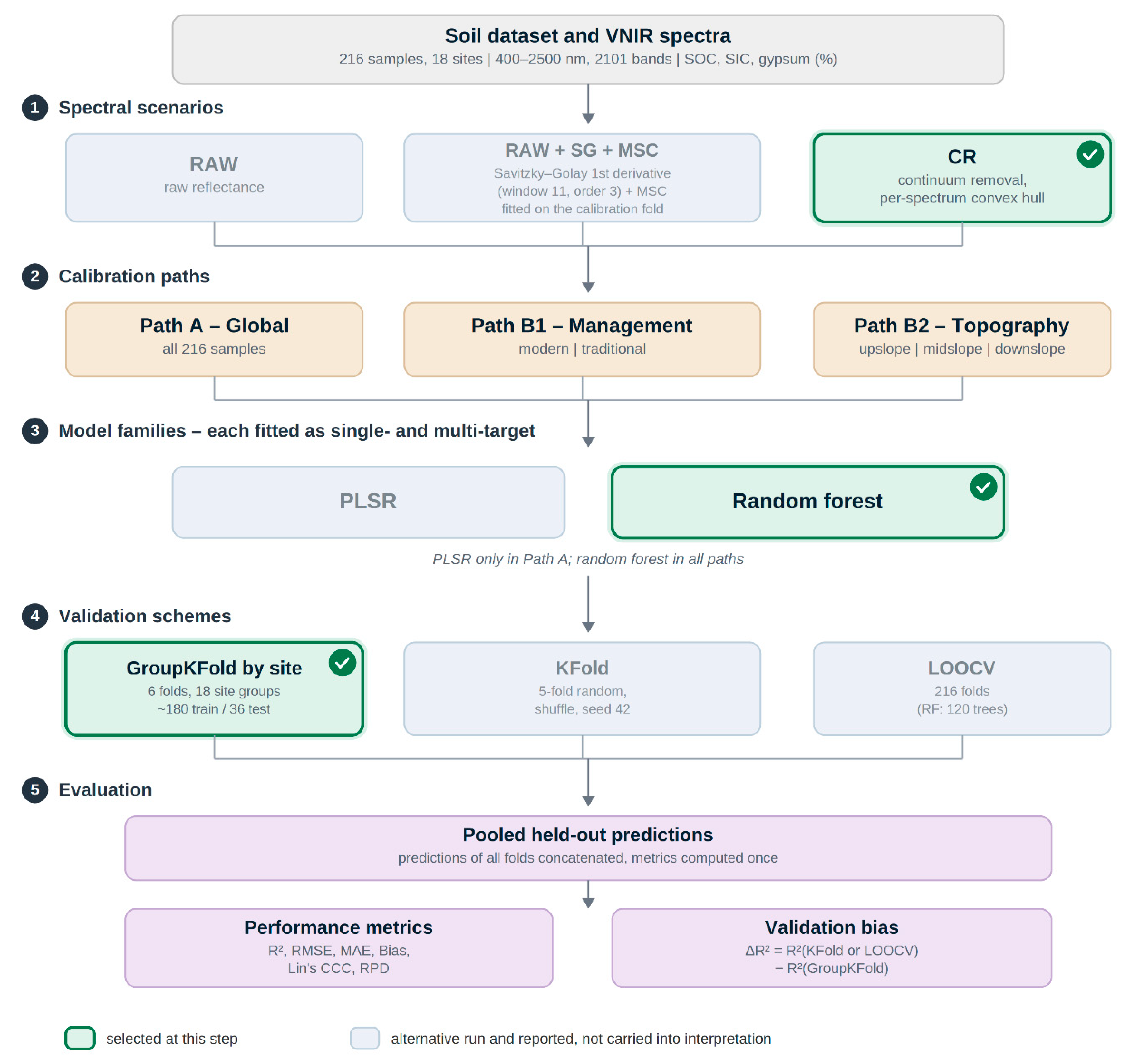
Figure 2.
Distribution of SOC, SIC, and gypsum across topography, soil depth, and oasis management.
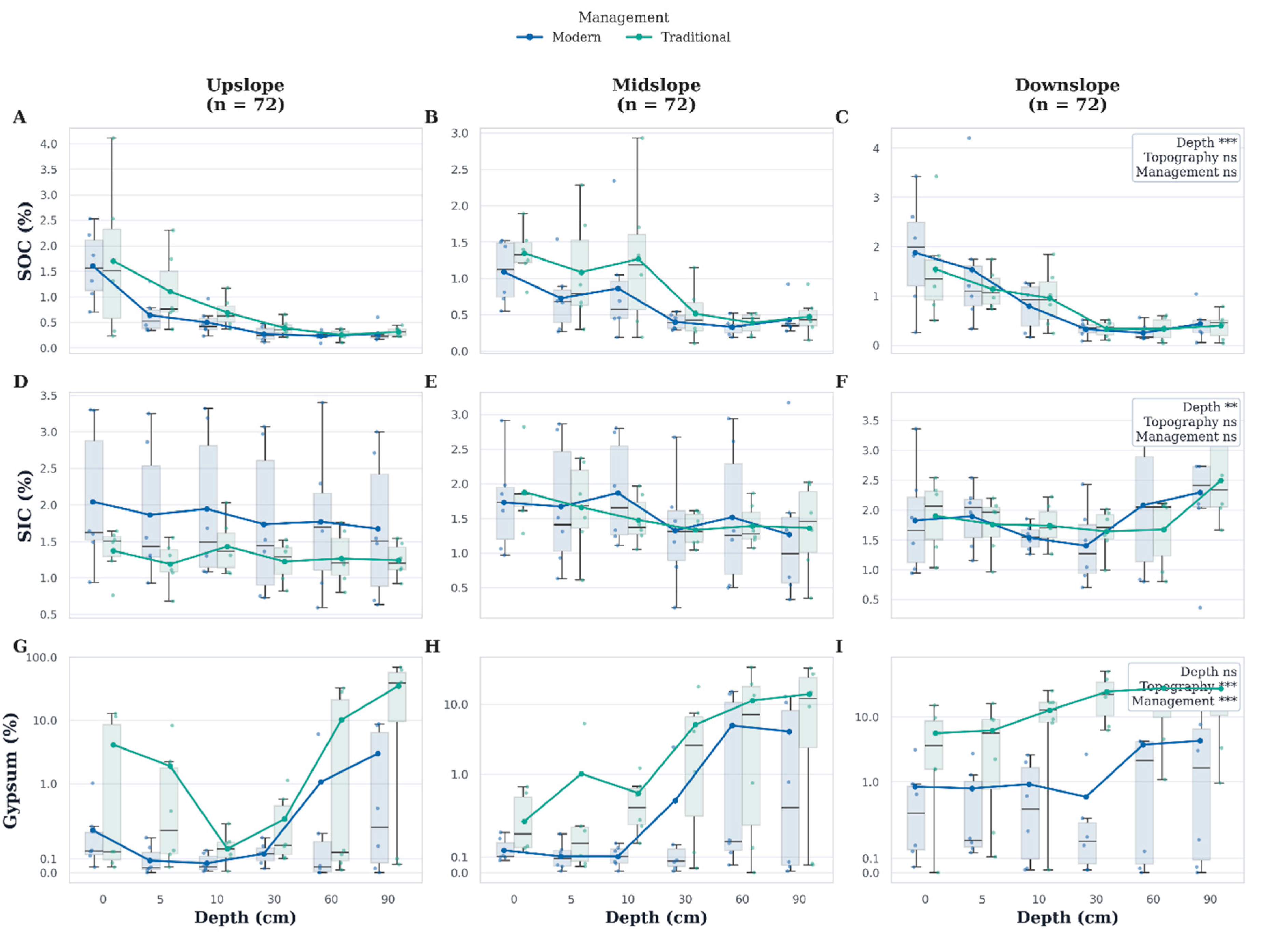
Figure 3.
Principal component analysis of VNIR spectra.
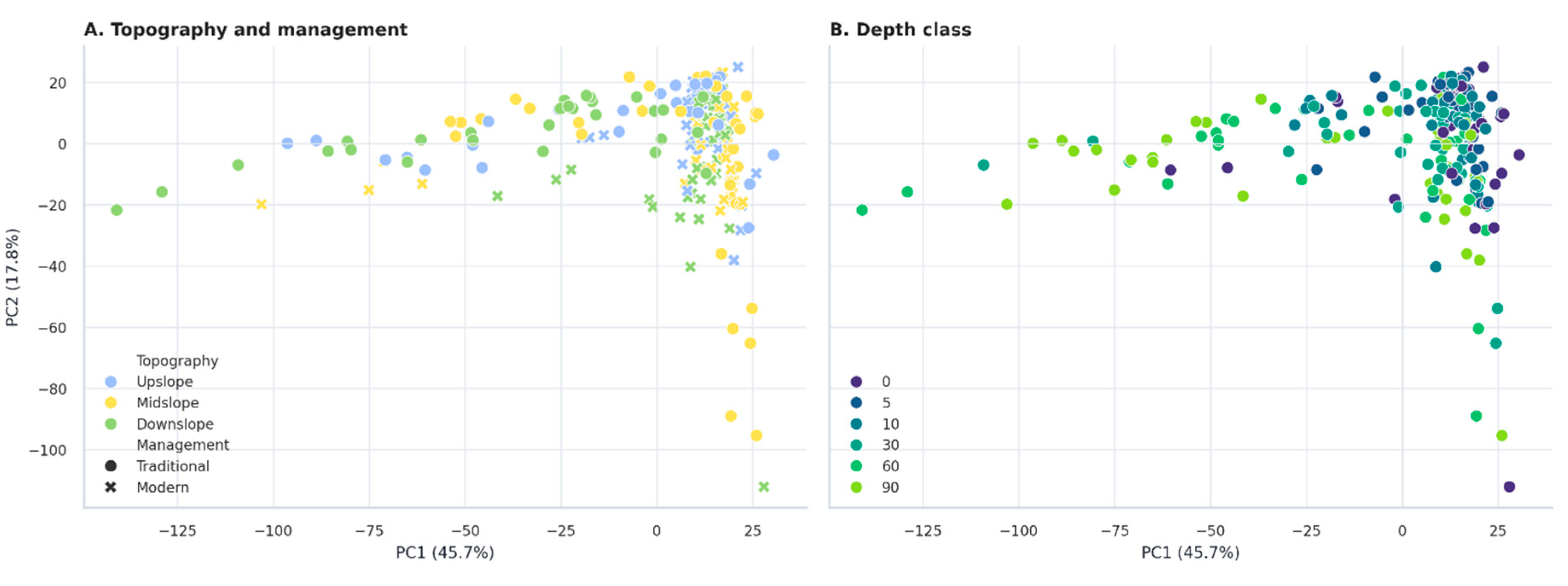
Figure 4.
Effects of validation strategy on RF model performance across global and stratified modelling pathways. R² values are shown for global, management-stratified, and topography-stratified RF models evaluated using plot-based GroupKFold, random KFold, and leave-one-out cross-validation (LOOCV). GroupKFold generally yielded more conservative performance estimates, particularly for SIC. Abbreviations: RF, random forest; SOC, soil organic carbon; SIC, soil inorganic carbon; LOOCV, leave-one-out cross-validation.
Figure 4.
Effects of validation strategy on RF model performance across global and stratified modelling pathways. R² values are shown for global, management-stratified, and topography-stratified RF models evaluated using plot-based GroupKFold, random KFold, and leave-one-out cross-validation (LOOCV). GroupKFold generally yielded more conservative performance estimates, particularly for SIC. Abbreviations: RF, random forest; SOC, soil organic carbon; SIC, soil inorganic carbon; LOOCV, leave-one-out cross-validation.
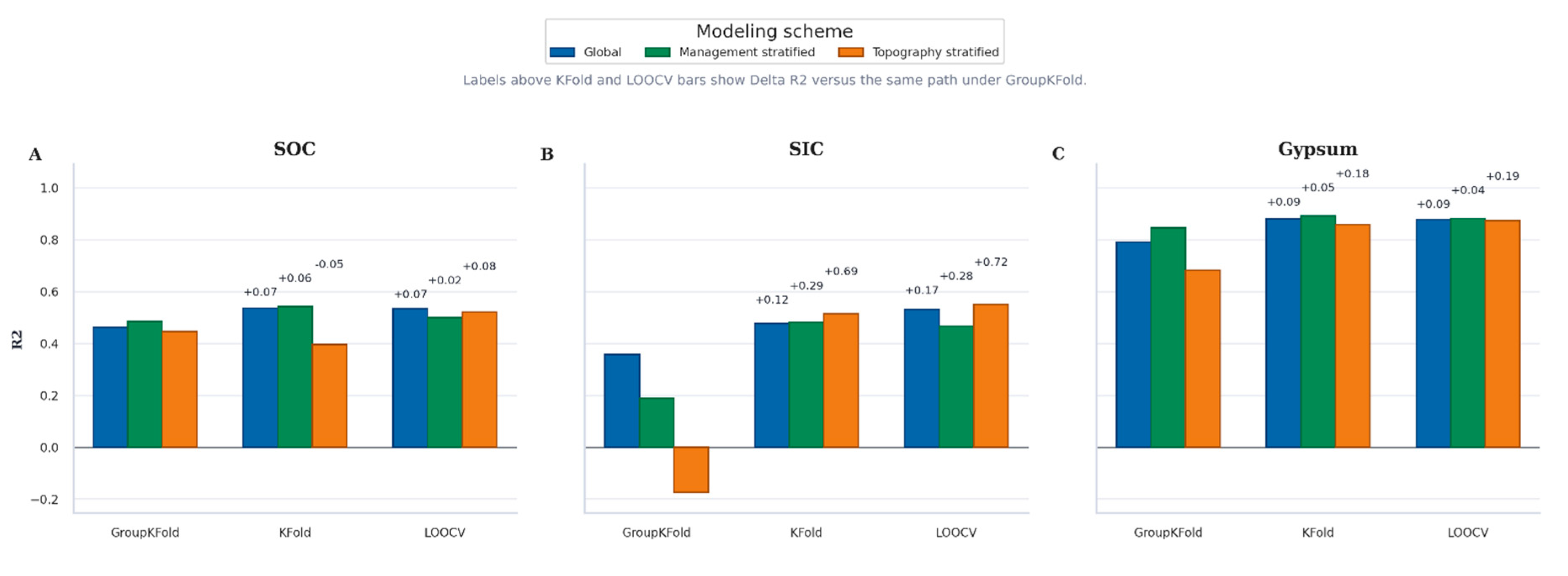
Figure 5.
Wavelength importance for RF prediction of SOC, SIC, and gypsum based on mean absolute SHAP values. The five most important wavelengths are shown for the best-performing RF configuration within each target and preprocessing variant. a–c, continuum-removed spectra (CR); d–f, Savitzky–Golay first-derivative preprocessing with multiplicative scatter correction (RAW+SG+MSC). Bar colours distinguish single-target and multi-target RF models, and R² and RMSE are reported in each panel. Higher mean absolute SHAP values indicate greater contributions of individual wavelengths to model predictions. Abbreviations: SHAP, Shapley additive explanations; RF, random forest; SOC, soil organic carbon; SIC, soil inorganic carbon; CR, continuum removal; SG, Savitzky–Golay; MSC, multiplicative scatter correction.
Figure 5.
Wavelength importance for RF prediction of SOC, SIC, and gypsum based on mean absolute SHAP values. The five most important wavelengths are shown for the best-performing RF configuration within each target and preprocessing variant. a–c, continuum-removed spectra (CR); d–f, Savitzky–Golay first-derivative preprocessing with multiplicative scatter correction (RAW+SG+MSC). Bar colours distinguish single-target and multi-target RF models, and R² and RMSE are reported in each panel. Higher mean absolute SHAP values indicate greater contributions of individual wavelengths to model predictions. Abbreviations: SHAP, Shapley additive explanations; RF, random forest; SOC, soil organic carbon; SIC, soil inorganic carbon; CR, continuum removal; SG, Savitzky–Golay; MSC, multiplicative scatter correction.
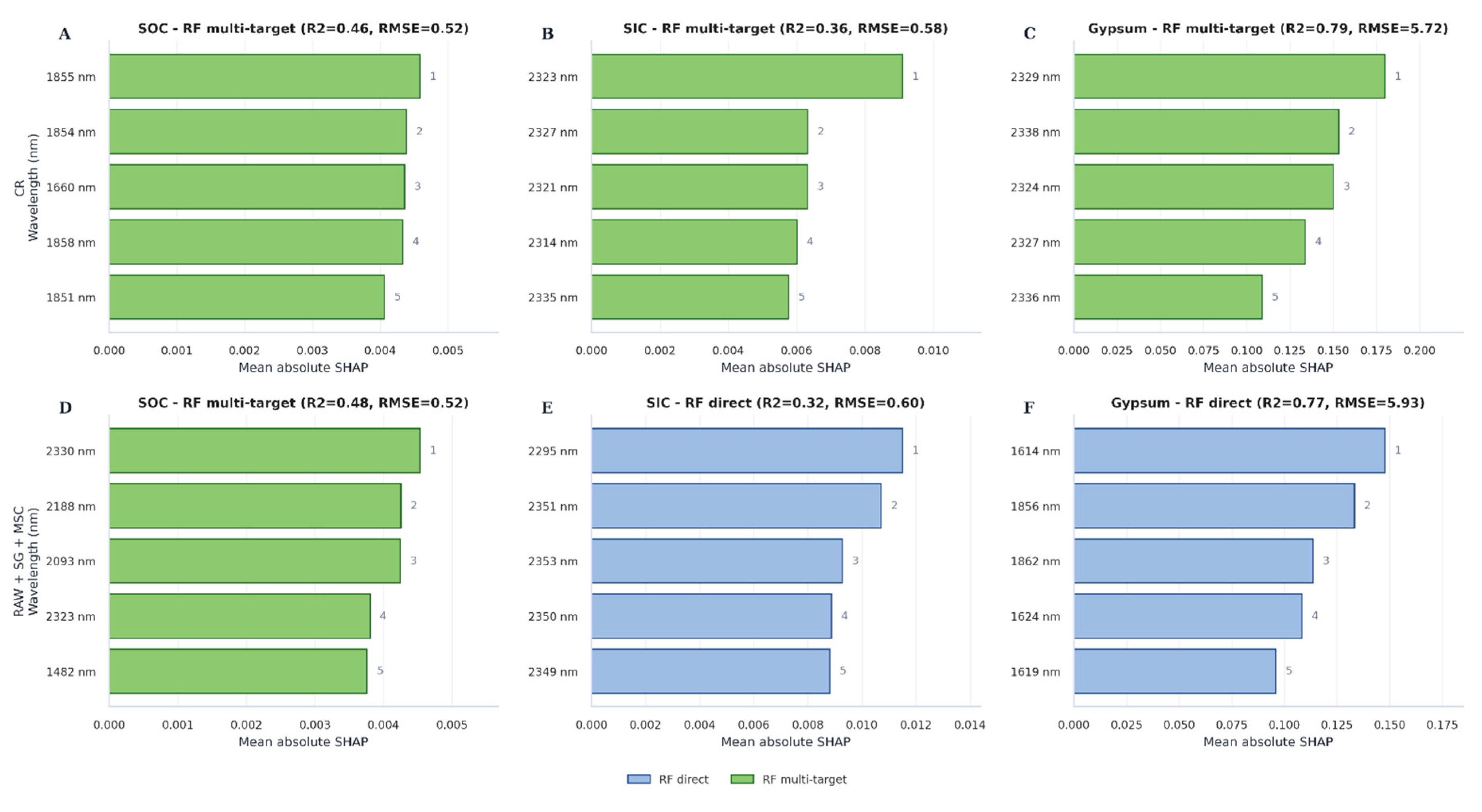

Table 1.
Plot-based GroupKFold validation performance of global PLSR and RF models for SOC, SIC, and gypsum using single- and multi-target workflows. Metrics were calculated from pooled held-out predictions. RMSE, MAE, and bias are expressed as % dry soil mass for all three target properties. Negative R² values indicate performance worse than prediction of the held-out mean. Abbreviations: SOC, soil organic carbon; SIC, soil inorganic carbon; PLSR, partial least squares regression; RF, random forest; R², coefficient of determination; RMSE, root mean square error; MAE, mean absolute error; CCC, concordance correlation coefficient; RPD, ratio of performance to deviation.
Table 1.
Plot-based GroupKFold validation performance of global PLSR and RF models for SOC, SIC, and gypsum using single- and multi-target workflows. Metrics were calculated from pooled held-out predictions. RMSE, MAE, and bias are expressed as % dry soil mass for all three target properties. Negative R² values indicate performance worse than prediction of the held-out mean. Abbreviations: SOC, soil organic carbon; SIC, soil inorganic carbon; PLSR, partial least squares regression; RF, random forest; R², coefficient of determination; RMSE, root mean square error; MAE, mean absolute error; CCC, concordance correlation coefficient; RPD, ratio of performance to deviation.
| Pathway | Target | Model | Flow | R2 | RMSE | MAE | Bias | CCC | RPD |
|---|---|---|---|---|---|---|---|---|---|
| Global | SOC | PLSR | direct | 0.34 | 0.78 | 0.60 | -0.02 | 0.48 | 0.91 |
| PLSR | multi | 0.35 | 0.74 | 0.53 | -0.06 | 0.52 | 0.96 | ||
| RF | direct | 0.43 | 0.54 | 0.35 | 0.06 | 0.66 | 1.32 | ||
| RF | multi | 0.46 | 0.52 | 0.34 | 0.00 | 0.63 | 1.36 | ||
| SIC | PLSR | direct | -0.08 | 0.85 | 0.66 | -0.09 | 0.32 | 0.86 | |
| PLSR | multi | -0.41 | 0.84 | 0.66 | -0.05 | 0.32 | 0.87 | ||
| RF | direct | 0.30 | 0.61 | 0.46 | -0.05 | 0.48 | 1.20 | ||
| RF | multi | 0.36 | 0.58 | 0.46 | -0.06 | 0.54 | 1.25 | ||
| Gypsum | PLSR | direct | 0.52 | 9.67 | 6.16 | 0.99 | 0.76 | 1.29 | |
| PLSR | multi | 0.65 | 9.03 | 5.78 | 0.85 | 0.75 | 1.38 | ||
| RF | direct | 0.79 | 5.73 | 2.73 | 0.14 | 0.88 | 2.18 | ||
| RF | multi | 0.79 | 5.72 | 2.72 | 0.19 | 0.88 | 2.18 |
Table 2.
Plot-based GroupKFold performance of RF models within management and topographic strata. Separate RF models were fitted for modern and traditional oasis systems and for upslope, midslope, and downslope positions using single- and multi-target workflows. Metrics were calculated from pooled held-out predictions within each stratum. RMSE, MAE, and bias are expressed as % dry soil mass for SOC, SIC, and gypsum. Negative R² values indicate performance worse than prediction of the held-out mean. Abbreviations: RF, random forest; SOC, soil organic carbon; SIC, soil inorganic carbon; R², coefficient of determination; RMSE, root mean square error; MAE, mean absolute error; CCC, concordance correlation coefficient; RPD, ratio of performance to deviation.
Table 2.
Plot-based GroupKFold performance of RF models within management and topographic strata. Separate RF models were fitted for modern and traditional oasis systems and for upslope, midslope, and downslope positions using single- and multi-target workflows. Metrics were calculated from pooled held-out predictions within each stratum. RMSE, MAE, and bias are expressed as % dry soil mass for SOC, SIC, and gypsum. Negative R² values indicate performance worse than prediction of the held-out mean. Abbreviations: RF, random forest; SOC, soil organic carbon; SIC, soil inorganic carbon; R², coefficient of determination; RMSE, root mean square error; MAE, mean absolute error; CCC, concordance correlation coefficient; RPD, ratio of performance to deviation.
| Target | Path | Stratum | Mode | N samples | R2 | RMSE | MAE | Bias | CCC | RPD |
|---|---|---|---|---|---|---|---|---|---|---|
| SOC | Management-stratified | Modern | direct | 108 | 0.41 | 0.54 | 0.34 | 0.03 | 0.63 | 1.31 |
| multi-target | 108 | 0.39 | 0.55 | 0.35 | 0.01 | 0.59 | 1.28 | |||
| Traditional | direct | 108 | 0.55 | 0.48 | 0.34 | 0.07 | 0.71 | 1.49 | ||
| multi-target | 108 | 0.48 | 0.52 | 0.36 | 0.03 | 0.62 | 1.38 | |||
| Topography-stratified | Upslope | direct | 72 | 0.38 | 0.56 | 0.38 | 0.13 | 0.60 | 1.27 | |
| multi-target | 72 | 0.36 | 0.56 | 0.39 | 0.13 | 0.56 | 1.25 | |||
| Midslope | direct | 72 | 0.54 | 0.39 | 0.27 | 0.07 | 0.70 | 1.48 | ||
| multi-target | 72 | 0.55 | 0.39 | 0.27 | 0.04 | 0.68 | 1.50 | |||
| Downslope | direct | 72 | 0.43 | 0.62 | 0.42 | 0.06 | 0.62 | 1.33 | ||
| multi-target | 72 | 0.35 | 0.66 | 0.46 | -0.03 | 0.49 | 1.24 | |||
| SIC | Management-stratified | Modern | direct | 108 | 0.30 | 0.73 | 0.54 | -0.08 | 0.48 | 1.20 |
| multi-target | 108 | 0.31 | 0.73 | 0.55 | -0.07 | 0.51 | 1.21 | |||
| Traditional | direct | 108 | -0.18 | 0.57 | 0.45 | -0.09 | 0.02 | 0.92 | ||
| multi-target | 108 | -0.25 | 0.58 | 0.46 | -0.10 | -0.13 | 0.90 | |||
| Topography-stratified | Upslope | direct | 72 | -0.37 | 0.87 | 0.62 | -0.16 | -0.12 | 0.85 | |
| multi-target | 72 | -0.19 | 0.81 | 0.57 | -0.14 | -0.01 | 0.92 | |||
| Midslope | direct | 72 | -0.53 | 0.85 | 0.66 | -0.20 | -0.18 | 0.81 | ||
| multi-target | 72 | -0.40 | 0.82 | 0.62 | -0.21 | -0.14 | 0.85 | |||
| Downslope | direct | 72 | -0.39 | 0.83 | 0.62 | 0.10 | -0.12 | 0.85 | ||
| multi-target | 72 | -0.09 | 0.74 | 0.56 | 0.12 | 0.05 | 0.96 | |||
| Gypsum | Management-stratified | Modern | direct | 108 | 0.79 | 1.54 | 0.76 | -0.01 | 0.87 | 2.18 |
| multi-target | 108 | 0.79 | 1.55 | 0.78 | -0.06 | 0.87 | 2.17 | |||
| Traditional | direct | 108 | 0.82 | 6.79 | 4.18 | 0.23 | 0.90 | 2.38 | ||
| multi-target | 108 | 0.82 | 6.77 | 4.21 | 0.24 | 0.90 | 2.38 | |||
| Topography-stratified | Upslope | direct | 72 | 0.72 | 7.01 | 2.96 | -0.84 | 0.80 | 1.90 | |
| multi-target | 72 | 0.72 | 6.98 | 2.94 | -0.85 | 0.81 | 1.91 | |||
| Midslope | direct | 72 | 0.50 | 5.33 | 2.85 | 0.26 | 0.66 | 1.41 | ||
| multi-target | 72 | 0.52 | 5.23 | 2.82 | 0.28 | 0.67 | 1.44 | |||
| Downslope | direct | 72 | 0.66 | 8.54 | 5.20 | -1.57 | 0.75 | 1.71 | ||
| multi-target | 72 | 0.66 | 8.54 | 5.22 | -1.55 | 0.75 | 1.71 |
Disclaimer/Publisher’s Note: The statements, opinions and data contained in all publications are solely those of the individual author(s) and contributor(s) and not of MDPI and/or the editor(s). MDPI and/or the editor(s) disclaim responsibility for any injury to people or property resulting from any ideas, methods, instructions or products referred to in the content. |
© 2026 by the authors. Licensee MDPI, Basel, Switzerland. This article is an open access article distributed under the terms and conditions of the Creative Commons Attribution (CC BY) license (http://creativecommons.org/licenses/by/4.0/).
Copyright: This open access article is published under a Creative Commons CC BY 4.0 license, which permit the free download, distribution, and reuse, provided that the author and preprint are cited in any reuse.