
Submitted:
03 September 2026
Posted:
04 September 2026
You are already at the latest version
Abstract
Automated sleep stage classification based on single channel EEG is a promising pathway to large-scale sleep monitoring outside the polysomnographic lab. This paper proposes SleepEffFormer TAS, an efficient and interpretable system that consists of a four-stride block 1D CNN feature extractor, two layers of pre-normalization Transformer encoder, and a non-parametric Transition-Aware Smoothing (TAS) layer that suppresses physio- logically unrealistic transitions between predicted stages. When tested on the Sleep EDF Expanded dataset (78 all-night EEG recordings, Fpz-Cz channel, subject-wise held-out split), the proposed model reaches 83.9% accuracy, 78.9% macro F1 score, and Cohen’s κ of 0.765 with around 367 K learnable parameters, performance comparable to AttnSleep while using 3–5× fewer parameters. Ablation study confirms that the Transformer encoder brings a performance improvement of 6.6 pp in macro F1 over a CNN-based system, the TAS layer increases performance by 1.8 pp without any trainable parameters, and weighted loss is critical for the minority sleep stage N1 classification task. The attention maps generated by the proposed model reveal physiologically sensible sleep stage-related EEG features. The source code of this project is available at: https://github.com/Nishi-Kanta-Paul/SleepStage.
Keywords:
sleep stage classification
; single channel EEG
; transformer
; 1D CNN
; transition-aware smoothing
; lightweight deep learning
; explainability
; sleep EDF
1. Introduction
The sleep staging pipeline, with the cyclic alternation of Wake, N1, N2, N3, and REM sleep stages through the course of the night, is the basis of the clinical assessment of a number of disorders, such as insomnia, obstructive sleep apnoea, or narcolepsy [1]. The current gold standard polysomnography (PSG) requires overnight in-laboratory recording and manual annotation under the American Academy of Sleep Medicine (AASM) guidelines; it is costly, unaffordable in developing countries, and impractical for population-scale data collection [2] needed for sleep studies with large cohorts.
Recent progress in automated deep learning sleep staging has been impressive. Deep convolutional neural networks have achieved state-of-the-art results by extracting spectro-temporal features directly from the signal without the need for feature engineering [2,3], while deep recurrent models account for the temporal structure inherent to sleep staging [5]. Recent research has further extended deep model expressiveness using self attention of intra epoch token sequences in transformers [4,6]. Despite these achievements, there still remain three practical issues. Firstly, efficient models have parameter budgets of several hundred thousands; hence they remain difficult to deploy on wearable or embedded devices. Secondly, transition insensitive classifiers may produce physiologically implausible stage transitions and thereby degrade hypnograms. Thirdly, the black box nature of most modern deep models hinders their widespread adoption in clinical applications.
These problems are addressed here through the following contributions:
- 1.
- SleepEffFormer TAS: a sub-400 K parameter EEG staging model which utilizes a lightweight 1D CNN tokeniser and a small Transformer encoder with 2 pre-norm layers.
- 2.
- Transition-Aware Smoothing (TAS): a parameter-free majority voting post-processing procedure that suppresses isolated, physiologically implausible stage transitions in the predicted sequence (+1.8 pp macro F1).
- 3.
- Attention-based explainability: stage-specific attention maps which identify EEG waveforms in each stage without changing model structure.
All proposed techniques are evaluated on the 78-recording Sleep EDF Expanded dataset.
The rest of this paper is organised as follows. Section 2 outlines the existing literature on convolutional, recurrent and attention-based sleep staging. Section 3 describes the proposed SleepEffFormer TAS architecture, the transition-aware smoothing layer and the attention-based explainability method. Section 4 covers the dataset, the experimental settings and the baseline methods. Section 5 presents the overall performance, per-class results and ablation study, while Section 6 draws the conclusions.
2. Related Work
2.1. CNNs and RNNs
The canonical CNN-RNN architecture demonstrated that it is feasible to perform end-to-end sleep staging from raw EEG without the need for hand-crafted features. For instance, DeepSleepNet [2] used parallel multi-scale CNN branches with small kernels for spindles and large kernels for slow-wave activity, followed by a BiLSTM with inter-epoch context modelling. SeqSleepNet [5] extended this by modelling sequences of 25 consecutive epochs, providing consistent gain for transitional stages. IITNet [7] modelled both intra- and inter-epoch dynamics in the shared recurrent network, showing that inter-epoch dynamics are especially effective in recognizing N1 and REM stages, where local features may be ambiguous. TinySleepNet [3] further optimized the CNN-LSTM architecture by using one large kernel CNN with a compact BiLSTM, demonstrating competitive accuracy with significantly fewer parameters. Early evidence of the efficiency accuracy trade-off which directly inspired the present work.
2.2. Attention Based Self Attention Staging
The arrival of self attention models in sleep staging aimed to address two problems with conventional LSTM-based architectures: sequential processing and lack of interpretability. AttnSleep [4] combined a multi-scale CNN encoder with a multi head self attention module, producing state-of-the-art results on Sleep EDF Expanded along with interpretable attention maps. SleepTransformer [6] introduced uncertainty quantification by applying Monte Carlo dropout to a Transformer architecture, resulting in improved reliability on transition stages. EEG-Conformer [8] introduced Conformer blocks combining convolutions and self attention, suitable for general-purpose EEG signal decoding tasks. L-SeqSleepNet [9] took this further, introducing efficient positional encoding mechanisms to model overnight recordings with near sub quadratic computation cost relative to sequence length. Finally, BIOT [10] introduced large-scale pre training of biosignal sequences for transfer-based sleep staging with minimal task-specific training data. These results show the utility of self attention based architectures in sleep staging; however, the present study shows that a light and trainable two-layer attention-based architecture is comparable in performance to heavier approaches when coupled with proper handling of class imbalance and post-processing smoothing.
2.3. Lightweight Models and Post-Processing
The lightweight nature of the wearable or point-of-care deployment requires small model sizes and deterministic inference latency. Recently, several studies [11,12] have addressed this challenge, where heterogeneous kernels in [11] were used to incorporate multi-scale features into a sub-200 K parameter network, and self-supervised pre training [12] enhanced the ability to learn rare sleep stages from limited data without changing the network size at inference time. As far as post-processing goes, hidden Markov models (HMMs), that make use of output distributions of classifiers [5], are well known to increase coherency of hypnograms, whereas Viterbi decoding with physiological transition matrices provides a principled probabilistic approach to the problem. While a simple majority voting-based approach has been somewhat overlooked, as it does not introduce any parameters nor requires estimation of a prior for transition probabilities, U-Sleep [13] illustrates cross-dataset robustness of a fully convolutional model. The contribution of this paper consists in comparing empirically two post-processing approaches: majority vote TAS vs Viterbi smoothing on the same hold out dataset, Sleep EDF Expanded.
3. Proposed Framework
3.1. Formulating the Problem
Consider a single channel 30-second EEG signal (100 Hz, Fpz-Cz). The proposed network outputs the label in accordance with the AASM manual (R&K stages 3 and 4 are combined in N3). The network is trained epoch-wise; therefore, the activation memory does not depend on the signal duration. Only the non-parametric TAS stage of Section 3.3 considers the entire per-subject sequence .
3.2. Architectural Design
Figure 1 shows the complete SleepEffFormer TAS framework. The architecture involves three trainable components, i.e., CNN feature extractor, Transformer encoder, and classifier, followed by a non-trainable component, i.e., TAS post processor.
3.2.1. 1D CNN Feature Extractor: Four Strided Conv1d Layers
A 3000-point-long signal is encoded into a sequence of 94 latent tokens with -dimensional features:
Increasing widths are: ; kernel sizes ; strides . The architecture of each block is Conv1d + BatchNorm1d + GELU. Writing , block computes
where denotes the stride- convolution with zero-padding , and the output length decreases from (Table 1). The total stride is 32, i.e. one token corresponds to seconds. The recursion
yields samples, so each token summarises a s EEG window, which is large enough to hold a sleep spindle burst or a K-complex. Strided convolution is used instead of max-pooling to pass gradient information through the entire receptive field.
3.2.2. Positional Encodings & Transformer Encoder
Sinusoidal positional encodings are added to and passed through a two-layer pre-normalisation Transformer encoder [15]:
Self attention is permutation-invariant; therefore, the order information is added by fixed sinusoidal encodings with alternating phase (sine/cosine), without adding parameters. As opposed to the original Post-LN implementation, Pre-LN normalises each sublayer (multi head attention and feed-forward) separately. Each of the two blocks evaluates
with a two-layer perceptron using GELU, and the i-th attention head given by
in which and come from linear projections of the normalised input, and the h heads are concatenated before a final projection by . Attention heads count is set to (); feed-forward layers use ; residual dropout is 0.1. Ensuring that the residual path is not normalised, the Pre-LN model can be trained without a warm-up schedule. With , the quadratic attention term ( M multiply-accumulate per block) is well below the projection and feed-forward terms ( M), so the dense attention is computationally feasible without any sparse approximation.
3.2.3. Classification Head
Global average pooling (GAP) of 94 positions yields a final 128-dimensional epoch embedding with ; this costs no parameters and lets every token count equally. Dropout(0.25) + linear classification leads to logits:
3.2.4. Objective Function
Imbalanced N1 data (comprising only around 5% of total epochs) is tackled using weighted cross-entropy. Inverse class frequency is used to compute per-class weightings, normalised such that their total sums up to :
with the empirical frequency of class c in the training split. According to the stage distribution of Section IV-A, this means that the N1 weight is about nine times the N2 weight; this accounts for the N1 recall reported in Section 5.4. On the whole, CNN tokenisation includes 101.6 K parameters (27.7%), the encoder 265.2 K (72.2%) and the classifier 0.6 K, totalling 367.5 K. Training procedure relies on AdamW (, ), and employs CosineAnnealingLR () with early stopping based on macro F1 scores of the validation set (patience of 15).
3.3. Transition-Aware Smoothing (TAS)
Unconstrained epoch-level outputs might not respect natural transitions between stages. TAS uses a sliding majority vote with window size of on every subject’s full sequence of predictions:
The window gets truncated at the sequence ends and ties break in favour of , which ensures that TAS never outputs a label not present in the window. With it extends min: not too short to filter out short, sporadic flips, yet not too long to destroy genuine short bouts, with the time complexity per subject. TAS requires no extra parameters and adds negligible cost at inference, and is performed identically on each subject’s outputs. The ablation study (Section 5.4) further investigates the effect of Viterbi decoding with physiological transition matrix.
3.4. Explainability Through Attention
The attention weights obtained from the last layer of the Transformer model are averaged over the four heads and provide an importance score for each token. With the attention matrix of head i, the token score is , i.e. the mean attention received by token t. This set of 94 values is resampled to a total of 3000 samples using the calculated stride of the CNN (). A saliency map is obtained in the time domain on the raw EEG epoch.
4. Experimental Setup
4.1. Data Set and Preprocessing
The expanded version of the Sleep EDF dataset cassette is used [14], which includes 78 PSG recordings from 39 different subjects (sampled at 100 Hz, Fpz-Cz EEG channel). Epochs are extracted from recordings according to the expert annotations with a duration of 30 seconds. Movements and unknown epochs are excluded, and R&K stages 3/4 are unified into one stage (N3). Preprocessing involves applying a 4th order Butterworth bandpass filter (0.5–40 Hz) and per-epoch z-score normalisation. The obtained distribution among the stages is extremely imbalanced: N2 ≈47%, Wake and REM ≈18% each, N3 ≈12%, and N1 ≈5%.
4.2. Evaluation Protocol
A stratified subject-wise split is performed at the recording level: 55 recordings are used for training, 12 for validation and 11 for testing. The partitioning is subject-independent, i.e. every recording of a given subject is assigned to a single partition, so no subject appears in more than one set and no epoch-level leakage is possible [5]. The final results are computed on the 11 held-out test recordings, none of whose subjects is seen during training. The macro-averaged F1 score is chosen as the primary metric, which treats all classes equally in terms of their prevalence (i.e., it has uniform weighting).
4.3. Baselines
Three baseline models apply the exact same preprocessing, subject-wise splitting protocol, and class weighting approach:
- 1D CNN (≈102 K): a CNN feature extractor with a global average pooling layer and a linear classifier without any sequential context modeling.
- CNN-LSTM (≈267 K): the above CNN feature extractor followed by a two-layer bidirectional LSTM layer with hidden size , where Transformer is replaced by the LSTM.
- TinySleepNet-lite (≈381 K): a large-kernel CNN () followed by two convolution layers and one LSTM layer as described in [3].
5. Results and Discussion
5.1. Overall Performance
Table 2 shows the performance figures on the test set for all configurations. SleepEffFormer TAS (smoothed) performs best with 83.9% accuracy, macro F1 score of 78.9%, and of 0.765 among all configurations. The Transformer encoder obtains an improvement of +3.4 points in macro F1 over CNN-LSTM and +6.6 points over CNN only baseline, suggesting that self attention in intra epochs captures global features of the EEG sequence that are not captured by strided convolutions alone. The use of the additional parameter free module, TAS, improves macro F1 by +1.8 points without extra inference overhead.
5.2. Per-Class Analysis and the N1 Challenge
To determine the strengths and weaknesses of the model, the classwise F1 measures and a normalised confusion matrix on the test data are examined. Both are generated using the original model without TAS to be able to isolate its effect separately in Section 5.4.
Figure 2 shows per-class F1-scores for the raw model. Wake (F1 = 0.915) and N2 (F1 = 0.871) obtain the best scores because of distinct spectral features of these stages. Broadband activity in case of Wake and sleep spindles/K-complexes in case of N2. N3 (F1 = 0.814) utilizes the strong delta-band power. N1 obtains the lowest F1-score of 0.391 because of the absence of characteristic waveforms. The confusion matrix shown in Figure 3 confirms that 32% of N1 epochs are classified as N2 and 15% as Wake, because the feature space of those classes shares similarity at the beginning of each episode. However, this is not a model-specific issue as it is the general problem at the signal level; the ablation experiment (see Section 5.4) shows that switching off class-weighted loss results in a reduction of N1 F1-score below 0.30 because of this problem.
The bar chart in Figure 2 highlights the discrepancy in performance across stages very clearly. Wake, N2, and N3 stages clearly pass the macro F1 reference line of 0.771 (dashed) showing that these stages have the aggregate score. REM stage lies close to the reference threshold line and shows moderate spectral overlap with N1 in the vicinity of sleep-cycle boundaries. On the other hand, N1 is way below the dashed reference threshold and thus shows that it is responsible for the aggregate score deficit. A pattern seen consistently by multiple algorithms [4,6] due to signal ambiguity rather than a lack of model performance. This discrepancy motivates using macro F1 as the main evaluation metric because otherwise, the deficit would be entirely hidden behind reporting accuracy, N1 contributes less than 5% to total epochs.
The confusion matrix in Figure 3 provides an insight into classifier behaviour at the epoch level. Each cell of the confusion matrix shows the fraction of truly labeled epochs in a given class among predicted classes. It becomes possible to compare the classifier’s performance in the stages with varying proportion of true-labels. It is clear that the classifier performs well in separating Wake, N2, N3, and REM stages, as the diagonal of the matrix dominates for those stages. For the rest of the stages, especially N1, there is a considerable number of misclassification instances. N1 epochs get predominantly classified as N2, with a considerable portion of them as Wake. Such bidirectional leakage may result from the nature of N1 stage when the low amplitude mixed frequency EEG resembles the EEG of wakefulness at sleep onset, and early N2 stage later on. The clean N3 row suggests that the classifier exploits the high amplitude delta band energy in distinguishing N3, and the lack of off-diagonal mass in the REM row indicates that REM related EEG characteristics, such as sawtooth waves and low amplitude mixed frequency activity, remain discriminative in the single channel Fpz-Cz setup.
5.3. Training Dynamics
Figure 4 shows the training and validation losses across epochs. The model converges in roughly 38–42 epochs, after which early stopping kicks in. A slight divergence between the validation loss and the training loss begins at epoch 25, which is normal behaviour for a relatively small number of training epochs, about 50 K. Cosine annealing schedule helps in smoothing out the loss plateau at later stages of training while avoiding premature convergence by decay of the learning rate from to approximately .
5.4. Ablation Study
Table 3 shows the quantification of individual contributions. Omitting the Transformer encoder results in the highest decrease of −6.6 pp in macro F1, making self attention the main contributor to performance. Removing the class-weighted loss degrades performance by −4.7 pp, with N1 recall being affected the most strongly. Physiologically-aware Viterbi smoothing produces outputs close to TAS by a difference of only 0.4 pp in accuracy, showing both approaches as viable options, though the majority-vote solution is simpler, does not require any prior knowledge and performs slightly better on this particular dataset.
5.5. Comparison with Published Work
In terms of the performance-efficiency trade-off, the smoothed model (Accuracy 83.9%, F1 78.9%) is competitive with AttnSleep [4] (Accuracy 84.1%, F1 79.8%), but has approximately 3–5× fewer parameters (≈367 K vs. ∼1–2 M). When compared to TinySleepNet [3] on the 78-recording dataset (F1 78.1%, 25 epochs input length for contextual information), the raw epoch-wise result (F1 77.1%) forms a reasonable base for comparison, since TAS makes up most of the difference. Models trained on the full-night recordings, such as SleepTransformer [6] and L-SeqSleepNet [9], outperform the proposed model in terms of macro F1 score by leveraging several hundred epochs of information. On the whole, the results follow the recent trends toward parameter optimization [11,12], showing that a thoughtfully designed model can be competitive with heavier counterparts without requiring a pre training setup or multi-channel input.
6. Conclusions
This research paper has presented SleepEffFormer TAS, a lightweight and interpretable single channel EEG sleep stage classification system achieving 83.9% accuracy and 78.9% macro F1 score on the expanded Sleep EDF benchmark with just ≈367 K parameters. Two-layer pre-norm Transformer encoder acts as the primary performance booster, giving an increase of +6.6 pp over a CNN only version. The TAS module with no additional parameters mitigates physiologically unrealistic sleep stage transitions, resulting in +1.8 pp improvement. Training with weighted loss appears to be crucial for proper N1 stage recall, and attention visualization highlights physiologically plausible EEG patterns at the different stages without changes to the architecture. Future research will focus on expanding sequence modeling across epochs without limitations, evaluating transferability between subjects and datasets, and adapting for ambulatory EEG recordings.
References
- Berry, R. B.; Budhiraja, R.; Gottlieb, D. J.; et al. The AASM Manual for the Scoring of Sleep and Associated Events: Rules, Terminology and Technical Specifications, ver. 2.0; American Academy of Sleep Medicine: Darien, IL, 2012. [Google Scholar]
- Supratak, A.; Dong, H.; Wu, C.; Guo, Y. DeepSleepNet: A model for automatic sleep stage scoring based on raw single channel EEG. IEEE Trans. Neural Syst. Rehabil. Eng. 2017, vol. 25(no. 11), 1998–2008. [Google Scholar] [CrossRef] [PubMed]
- Supratak, A.; Guo, Y. TinySleepNet: An efficient deep learning model for sleep stage scoring based on raw single channel EEG. Proc. 42nd Annu. Int. Conf. IEEE Eng. Med. Biol. Soc. (EMBC), Montreal, Canada, 2020; pp. 641–644. [Google Scholar]
- Eldele, E.; Chen, Z.; Liu, C.; Wu, M.; Kwoh, C.-K.; Li, X.; Guan, C. An attention-based deep learning approach for sleep stage classification with single channel EEG. IEEE Trans. Neural Syst. Rehabil. Eng. 2021, vol. 29, 809–820. [Google Scholar] [CrossRef] [PubMed]
- Phan, H.; Andreotti, F.; Cooray, N.; Chen, O. Y.; De Vos, M. SeqSleepNet: End-to-end hierarchical recurrent neural network for sequence-to-sequence automatic sleep staging. IEEE Trans. Neural Syst. Rehabil. Eng. 2019, vol. 27(no. 3), 400–410. [Google Scholar] [CrossRef] [PubMed]
- Phan, H.; Chèn, O. Y.; Koch, P.; Mertins, A.; De Vos, M. SleepTransformer: Automatic sleep staging with interpretability and uncertainty quantification. IEEE Trans. Biomed. Eng. 2022, vol. 69(no. 8), 2456–2467. [Google Scholar] [CrossRef] [PubMed]
- Choi, S.; Ahn, S.; Park, S. Intra- and inter-epoch temporal context network (IITNet) using sub-epoch features for automatic sleep scoring on raw single channel EEG. Biomed. Signal Process. Control 2020, vol. 61, 102037. [Google Scholar] [CrossRef]
- Song, Y.; Zheng, Q.; Liu, B.; Gao, X. EEG-Conformer: Convolutional Transformer for EEG signal decoding and visualization. IEEE Trans. Neural Syst. Rehabil. Eng. 2022, vol. 31, 710–719. [Google Scholar] [CrossRef] [PubMed]
- Phan, H.; Mikkelsen, K.; Chèn, O. Y.; Koch, P.; Mertins, A.; Kidmose, P.; De Vos, M. L-SeqSleepNet: Whole-night long sequence modelling for automatic sleep staging. IEEE J. Biomed. Health Inform. 2023, vol. 27(no. 10), 4895–4904. [Google Scholar] [CrossRef] [PubMed]
- Yang, C.; Westover, M. B.; Sun, J. BIOT: Cross-data biosignal foundation model via multi-scale multi-period channel independence. Adv. Neural Inf. Process. Syst. (NeurIPS), New Orleans, LA, 2023. [Google Scholar]
- Ye, R.; Liu, H.; Zhang, L. MixSleepNet: Multi-type convolution kernel-based sleep stage classification model. Proc. 45th Annu. Int. Conf. IEEE Eng. Med. Biol. Soc. (EMBC), Sydney, Australia, 2023; pp. 1–5. [Google Scholar]
- Li, Y.; Wang, Z.; Pan, S. Self-supervised contrastive learning for automated sleep stage classification from EEG. Proc. IEEE Int. Conf. Acoust. Speech Signal Process. (ICASSP), Seoul, Korea, 2024; pp. 1–5. [Google Scholar]
- Perslev, M.; Darkner, S.; Kempfner, L.; Nikolic, M.; Jennum, P. J.; Igel, C. U-Sleep: Resilient high-frequency sleep staging. npj Digit. Med. 2021, vol. 4(no. 1), 72. [Google Scholar] [CrossRef] [PubMed]
- Goldberger, A. L.; Amaral, L. A. N.; Glass, L.; et al. PhysioBank, PhysioToolkit, and PhysioNet: Components of a new research resource for complex physiologic signals. Circulation 2000, vol. 101(no. 23), e215–e220. [Google Scholar]
- Xiong, R.; Yang, Y.; He, D.; et al. On layer normalization in the Transformer architecture. Proc. Int. Conf. Mach. Learn. (ICML) 2020, vol. 119, 10524–10533. [Google Scholar]
Figure 1.
SleepEffFormer TAS architecture. (a) End-to-end pipeline from raw epoch to hypnogram. (b) CNN tokeniser with per-block output shapes. (c) Pre-LN encoder block; the residual path bypasses each normalised sublayer. Dashed purple: attention-based saliency.
Figure 1.
SleepEffFormer TAS architecture. (a) End-to-end pipeline from raw epoch to hypnogram. (b) CNN tokeniser with per-block output shapes. (c) Pre-LN encoder block; the residual path bypasses each normalised sublayer. Dashed purple: attention-based saliency.
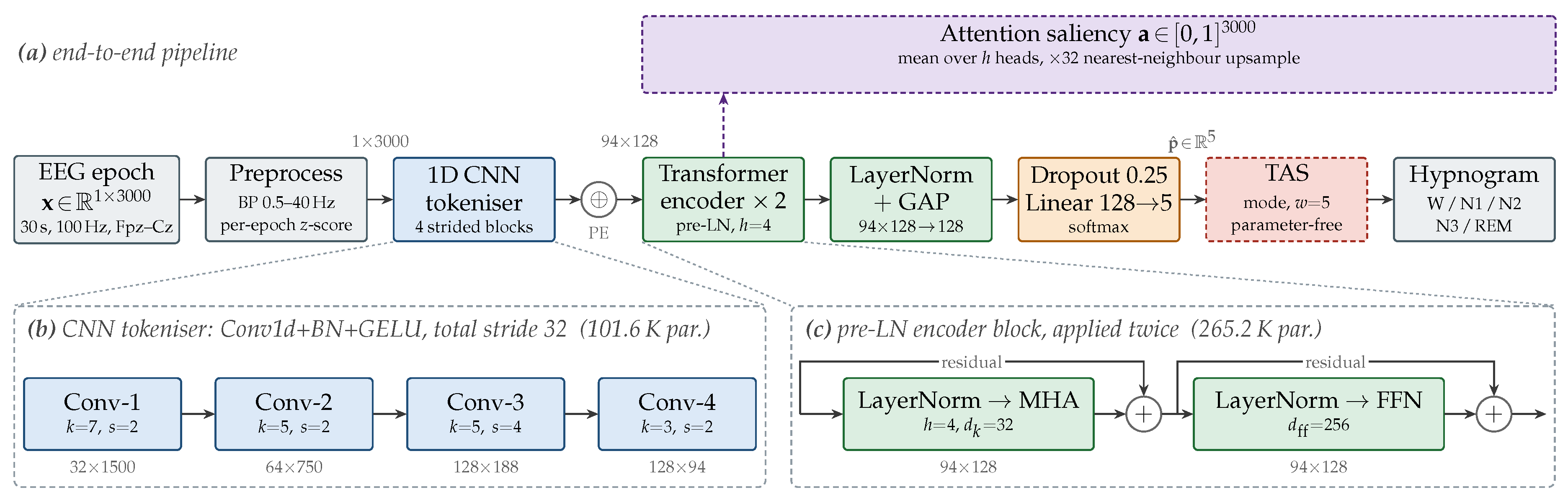
Figure 2.
Per-class F1 scores (raw model, no TAS). Dashed line: macro F1 = 0.771. N1 is conspicuously short (≈0.39) owing to its transitional spectral overlap with both Wake and N2.
Figure 2.
Per-class F1 scores (raw model, no TAS). Dashed line: macro F1 = 0.771. N1 is conspicuously short (≈0.39) owing to its transitional spectral overlap with both Wake and N2.
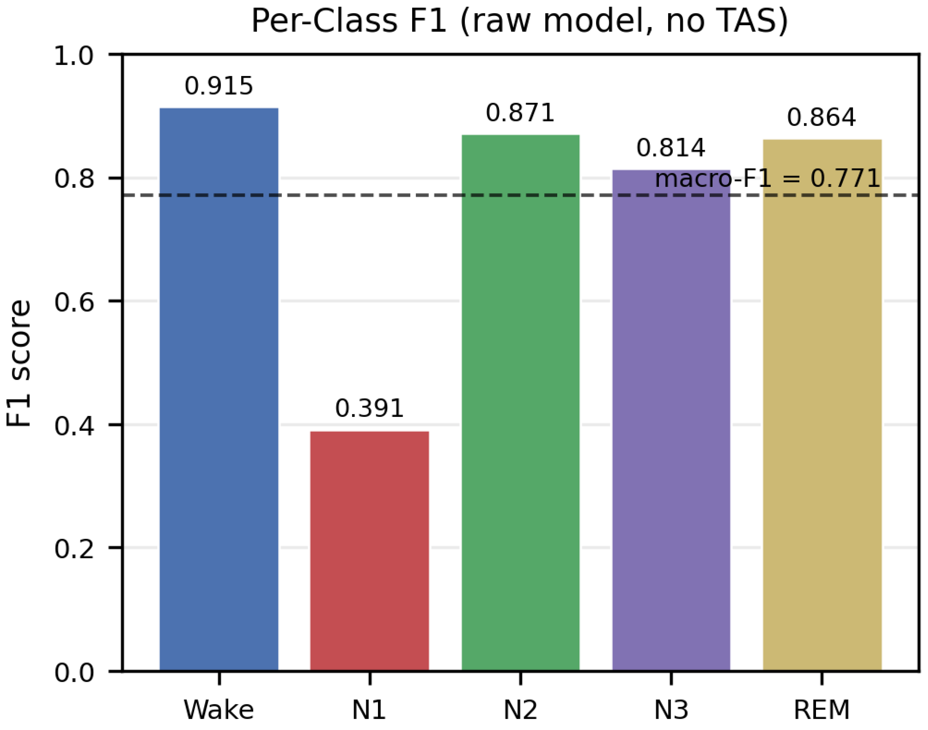
Figure 3.
Row-normalised confusion matrix on the test set (model without TAS). Each cell shows the row-normalised rate (top) and the raw epoch count (bottom); rates are derived from the counts. N1 is the weakest stage, with dominant confusions N1 → N2 (0.32) and N1 → Wake (0.15).
Figure 3.
Row-normalised confusion matrix on the test set (model without TAS). Each cell shows the row-normalised rate (top) and the raw epoch count (bottom); rates are derived from the counts. N1 is the weakest stage, with dominant confusions N1 → N2 (0.32) and N1 → Wake (0.15).
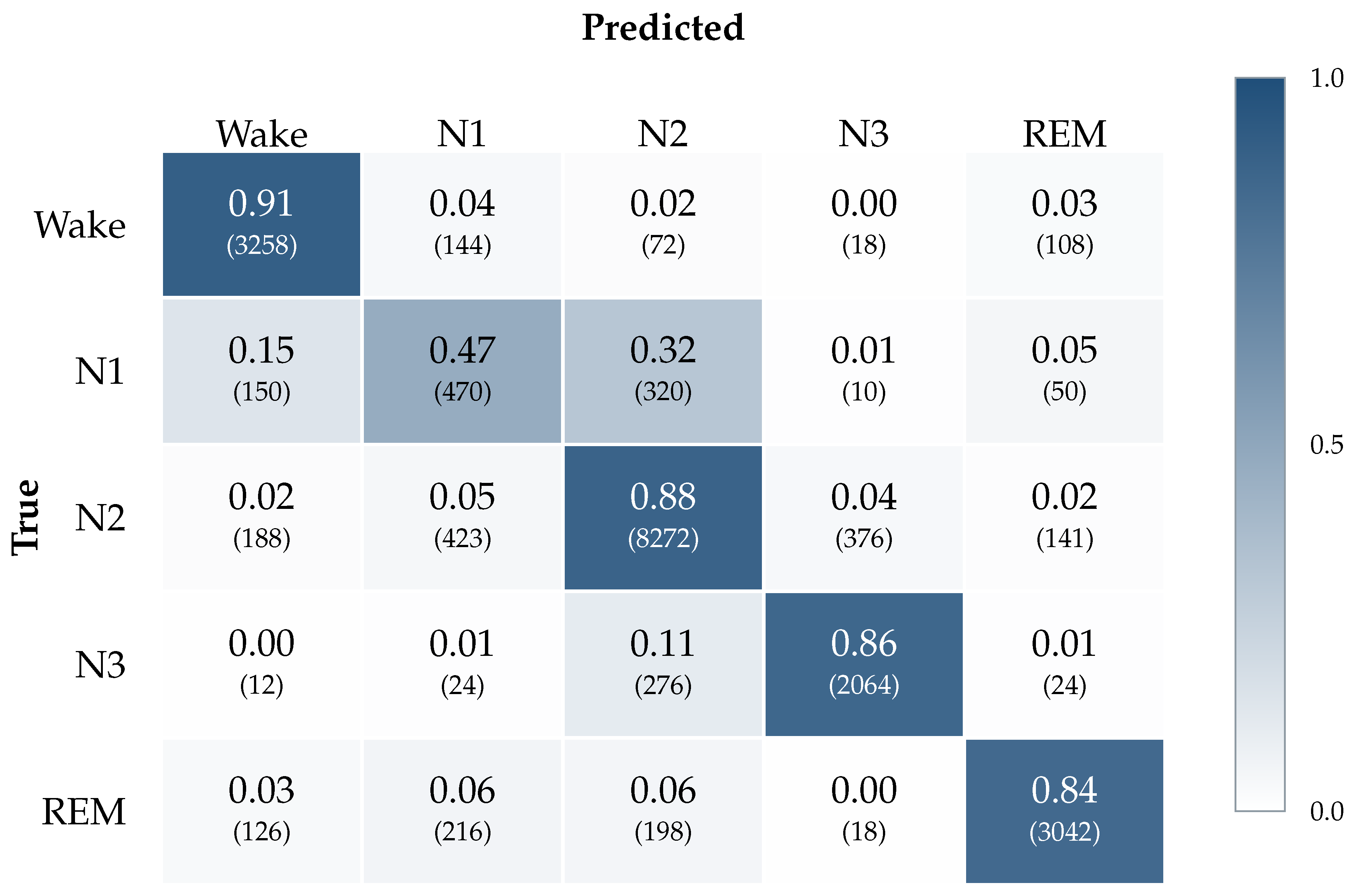
Figure 4.
Training (solid) and validation (dashed) loss curves. Early stopping fires at ≈ epoch 40 (patience = 15 on val macro F1). Mild divergence after epoch 25 reflects dataset size and is within normal range for Sleep EDF Expanded.
Figure 4.
Training (solid) and validation (dashed) loss curves. Early stopping fires at ≈ epoch 40 (patience = 15 on val macro F1). Mild divergence after epoch 25 reflects dataset size and is within normal range for Sleep EDF Expanded.
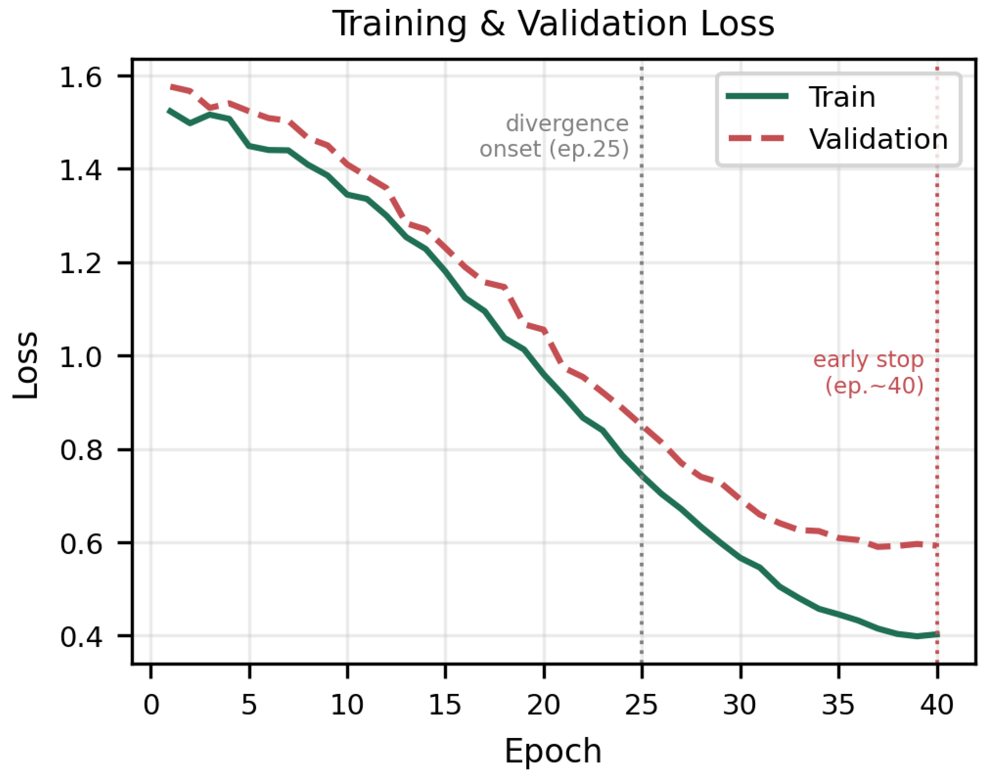

Table 1.
Layer-wise configuration of the SleepEffFormer TAS backbone for a single 30 s epoch at 100 Hz (). Here stands for kernel, stride and padding.
Table 1.
Layer-wise configuration of the SleepEffFormer TAS backbone for a single 30 s epoch at 100 Hz (). Here stands for kernel, stride and padding.
| Stage | Operation | Output | Params | |
|---|---|---|---|---|
| Input | raw EEG epoch | – | 0 | |
| Conv-1 | Conv1d+BN+GELU | 7/2/3 | 320 | |
| Conv-2 | Conv1d+BN+GELU | 5/2/2 | 10,432 | |
| Conv-3 | Conv1d+BN+GELU | 5/4/2 | 41,344 | |
| Conv-4 | Conv1d+BN+GELU | 3/2/1 | 49,536 | |
| PE | sinusoidal, additive | – | 0 | |
| Enc-1 | Pre-LN block, | – | 132,480 | |
| Enc-2 | Pre-LN block, | – | 132,480 | |
| LN | final LayerNorm | – | 256 | |
| GAP | mean over tokens | – | 128 | 0 |
| Head | Dropout(0.25)+Linear | – | 5 | 645 |
| TAS | sliding mode, | – | 5 | 0 |
| Total trainable | 367,493 | |||
Table 2.
Performance on the Sleep EDF Expanded test set. Best result in bold.
| Model | Acc. | F1mac | Params | |
|---|---|---|---|---|
| 1D CNN | 0.783 | 0.723 | 0.691 | 102 K |
| TinySleepNet-lite | 0.794 | 0.734 | 0.702 | 381 K |
| CNN-LSTM | 0.806 | 0.749 | 0.717 | 267 K |
| Proposed (raw) | 0.823 | 0.771 | 0.748 | 367 K |
| Proposed + TAS | 0.839 | 0.789 | 0.765 |
Table 3.
Ablation study: macro F1 on the test set.
| Configuration | F1mac | |
|---|---|---|
| Full model + TAS (majority vote) | 0.789 | — |
| Full model, no TAS | 0.771 | |
| TAS: Viterbi decoder | 0.785 | |
| No class-weighted loss | 0.742 | |
| No Transformer (1D CNN only) | 0.723 |
Disclaimer/Publisher’s Note: The statements, opinions and data contained in all publications are solely those of the individual author(s) and contributor(s) and not of MDPI and/or the editor(s). MDPI and/or the editor(s) disclaim responsibility for any injury to people or property resulting from any ideas, methods, instructions or products referred to in the content. |
© 2026 by the authors. Licensee MDPI, Basel, Switzerland. This article is an open access article distributed under the terms and conditions of the Creative Commons Attribution (CC BY) license (http://creativecommons.org/licenses/by/4.0/).
Copyright: This open access article is published under a Creative Commons CC BY 4.0 license, which permit the free download, distribution, and reuse, provided that the author and preprint are cited in any reuse.