

Submitted:
03 September 2026
Posted:
04 September 2026
You are already at the latest version
Abstract
Winter Storm Uri (February 2021) caused the largest power grid failure in Texas history, with extensive outages in the state's most populous Harris County. This study integrates NASA Black Marble VNP46A2 nighttime light (NTL) observations with the CDC Social Vulnerability Index (SVI) to characterize post-storm recovery across 1,070 census tracts. Recovery was defined as the first day tract-level NTL reached at least 90% of its pre-storm baseline for three consecutive days. Contrary to the expectation that vulnerable communities recover more slowly, spatial regression revealed a weak, statistically significant negative association between SVI and recovery time (β = −0.556, p = 0.050), with spatial dependence also significant (ρ ≈ 0.47). Local Indicators of Spatial Autocorrelation identified significant clusters of slow recovery in lower-SVI suburban areas and fast recovery in higher-SVI urban neighborhoods. This association was sensitive to the recovery definition, reversing signs under longer persistence requirements. The spatial organization of urban infrastructure, rather than vulnerability alone, may plausibly explain these patterns, though not directly testable with available data. These findings caution against assuming a universal vulnerability–recovery relationship in infrastructure disasters and highlight the sensitivity of nighttime-light-based equity assessments to how recovery is operationally defined.
Keywords:
Winter Storm Uri
; VIIRS nighttime lights
; spatial regression
; spatial autocorrelation
; urban recovery
; Social Vulnerability Index
; urban resilience
1. Introduction
Winter Storm Uri struck Texas in February 2021, bringing consecutive days of sub-freezing temperatures that triggered the largest power grid failure in the state's history. Electricity outages affected more than 4.5 million customers (an estimated 10 million residents) as the Electric Reliability Council of Texas (ERCOT) ordered massive load shedding to prevent a total grid collapse [1,2]. The crisis exposed structural vulnerabilities within the Texas electrical generation and distribution network, specifically the failure of natural gas supply lines and power plants to winterize against extreme cold [1]. Harris County, which contains the City of Houston and is the third most populous county in the United States, experienced disproportionately severe service disruptions: a University of Houston survey found that 91% of Harris County residents lost power at some point during the storm, compared with 64% across the rest of the state's electrical grid [3]. Statewide physical and economic damage exceeded an estimated $200 billion [4]. The loss of electrical power disabled water treatment plants, emergency medical services, and residential heating systems [1]. Tracking the spatial and temporal trajectories of post-disaster infrastructure recovery provides baseline data for emergency management planning and resilience assessment [5,6].
Socially vulnerable populations may experience worse hazard impacts and longer recovery periods [7,8]. The CDC/ATSDR Social Vulnerability Index (SVI) synthesizes socioeconomic and demographic indicators like income, household composition, minority status, and housing type to quantify community-level risk [9]. However, composite vulnerability indices carry inherent methodological uncertainty: index rankings can be sensitive to indicator selection, transformation method, and weighting scheme, and different construction choices can yield divergent vulnerability rankings for the same location [10,11]. Previous studies demonstrate that higher social vulnerability correlates with greater property damage and delayed housing recovery following extreme weather [12]. Displacement following disaster-driven housing loss can also impose lasting psychological burdens on low-income populations [13]. Energy insecurity research further shows that low-income and minority households disproportionately reside in older, poorly insulated housing stock, requiring more electricity to maintain safe indoor temperatures [14,15].
Most of this empirical evidence relies on hydrometeorological events like hurricanes and riverine flooding, where physical hazard exposure dictates the recovery timeline [12]. Whether these socioeconomic disparities persist during large-scale winter power grid failures remains an open empirical question.
Unlike flood or wind damage, power restoration follows centralized utility protocols, substation locations, and the physical topology of distribution feeders [16]. Standard utility restoration procedures prioritize critical facilities, such as hospitals and fire stations, and then attempt to maximize the number of customers reconnected per switching operation [17,18]. However, this strategy can structurally disadvantage suburban or rural communities located on lower-density, radial distribution lines [16,19]. Marginalized populations concentrated in high-density urban cores might experience faster physical grid restoration simply because they reside on high-capacity feeders near major substations. Aggregate county-level studies often fail to isolate this mechanical reality from socioeconomic factors [20].
Satellite-derived nighttime light (NTL) remote sensing provides a spatially continuous observational tool to track post-disaster recovery across large extents, bypassing the need for proprietary utility telemetry data [21,22]. The NASA Black Marble VNP46A2 product suite, derived from the Visible Infrared Imaging Radiometer Suite (VIIRS) Day/Night Band (DNB) on the Suomi-NPP satellite, provides daily NTL data at a 15 arc-second (approximately 500 m) spatial resolution [23,24]. The VNP46A2 product applies atmospheric and BRDF corrections and adjusts for lunar illumination, and its gap-filling algorithm supplies estimated radiance values for pixels affected by cloud or snow contamination [25,26,27].
Early remote sensing studies used NTL data primarily for rapid damage assessment or mapping discrete outage extents [28,29]. Disaster research now uses high-frequency daily NTL time series to track continuous recovery trajectories after hurricanes and earthquakes [27,30,31,32]. Isolating residential power restoration from commercial centers, industrial plants, or highway lighting remains difficult. Standard aggregate NTL metrics are easily skewed by brightly lit, non-residential facilities that retain power or operate heavy-duty backup generators [23]. Tracking residential recovery requires high-resolution land-cover masking and temporal smoothing techniques to separate the community recovery signal from commercial background noise [26,30].
Power restoration is a physical process dictated by grid wiring, meaning recovery outcomes are spatially dependent. Statistical models like ordinary least squares (OLS) regression assume independence among observations. This assumption fails in infrastructure recovery datasets due to shared distribution feeders and municipal utility boundaries [33,34]. Spatial econometric techniques, specifically Spatial Lag Models (SLM) and Spatial Error Models (SEM), incorporate spatial weight matrices to account for autocorrelation [33]. SLMs model the direct influence of neighboring tracts on each other, which aligns with the physical reality of adjacent neighborhoods sharing substations. Local Indicators of Spatial Autocorrelation (LISA) decompose these global patterns to detect statistically significant geographic clusters and spatial outliers [35]. These spatial econometric methods have rarely been paired with daily satellite NTL metrics to evaluate urban power grid restoration at the census-tract level [32].
Existing literature contains three specific limitations. First, while NTL is frequently used for outage mapping, few studies construct continuous, tract-level recovery metrics that filter out non-residential lighting artifacts using explicit land-cover masking [26,30]. Second, the empirical relationship between community social vulnerability and power restoration during winter blackouts is poorly understood in dense metropolitan areas, where high-capacity utility infrastructure might confound individual socioeconomic conditions [16,19]. Third, studies rarely integrate daily remote sensing metrics, standardized social vulnerability dimensions, and spatial econometric models to separate social vulnerability effects from the spatial autocorrelation of urban power grids [32,33].
This study integrates NASA Black Marble VNP46A2 daily NTL observations, the 2020 CDC/ATSDR SVI, and spatial econometric modeling to examine post-disaster recovery across 1,070 census tracts in Harris County following Winter Storm Uri. We specify four objectives: (1) calculate a continuous tract-level NTL recovery metric, Days to Power Restoration (DTR), using developed-land masking (NLCD 2019) and temporal smoothing algorithms; (2) evaluate the spatial relationship between social vulnerability themes and power restoration trajectories using Spatial Lag Models; (3) test whether pre-storm lighting intensity confounds the observed recovery times across different vulnerability tiers; and (4) map geographic clusters of fast and slow recovery using LISA analysis to assess spatial equity.
Section 2 details the study area, data sources, remote sensing preprocessing pipeline, and spatial modeling framework. Section 3 presents spatial autocorrelation tests, regression outputs, and LISA cluster distributions. Section 4 discusses the mechanisms driving the observed patterns and policy implications. Section 5 concludes.
2. Materials and Methods
2.1. Study Area
Figure 1 shows the location of Harris County, Texas, and the spatial distribution of the census tracts included in this study. Located in southeastern Texas, the county covers approximately 4,604 km². At the time of Winter Storm Uri in February 2021, it had an estimated population of approximately 4.74 million, making it the third most populous county in the United States [36].
The county exhibits pronounced socioeconomic heterogeneity, with highly vulnerable neighborhoods concentrated in the urban core of Houston and comparatively affluent communities distributed across the suburban periphery. Combined with its extensive urban power distribution network, these characteristics provide an appropriate setting for investigating spatial variations in post-disaster recovery. To capture neighborhood-scale recovery patterns, the 2020 U.S. Census tract was adopted as the fundamental spatial unit of analysis. Following data preprocessing and quality control procedures described in Section 2.3, the final analytical dataset comprised 1,070 census tracts. Since Winter Storm Uri, Harris County has continued to experience sustained population growth, reaching an estimated 5.05 million residents in 2025 [36], underscoring the continuing importance of understanding infrastructure resilience and post-disaster recovery in rapidly growing metropolitan regions in the United States.
2.2. Data Sources
This study integrates multiple remote sensing, socioeconomic, and geospatial datasets to quantify post-disaster nighttime light recovery and examine its relationship with social vulnerability. Table 1 summarizes the datasets used in this study.
2.2.1. NASA Black Marble Nighttime Light Data
Daily nighttime light observations were obtained from the NASA Black Marble VNP46A2 product [23] through Google Earth Engine (GEE). The dataset is derived from the Visible Infrared Imaging Radiometer Suite (VIIRS) Day/Night Band (DNB) and provides daily BRDF-corrected nighttime light observations at a native spatial resolution of approximately 500 m. The DNB_BRDF_Corrected_NTL band was used throughout this study because it corrects for atmospheric effects, lunar illumination, and bidirectional reflectance distribution function (BRDF) effects, thereby improving the temporal consistency of nighttime light observations. To ensure radiometric reliability while maintaining adequate temporal coverage, only pixels with Mandatory_Quality_Flag values of 0 (high quality) or 1 (gap-filled) were retained, whereas pixels with flag values of 2 and 3 were excluded.
2.2.2. CDC/ATSDR SVI
Social vulnerability was characterized using the CDC/ATSDR SVI 2020, which is derived from the 2016–2020 American Community Survey (ACS) 5-year estimates. The dataset provides percentile rankings for the overall SVI (RPL_THEMES) and four thematic dimensions, including socioeconomic status (RPL_THEME1), household characteristics (RPL_THEME2), racial and ethnic minority status (RPL_THEME3), and housing type and transportation (RPL_THEME4). All SVI values range from 0 to 1, with higher values indicating greater social vulnerability. Census tracts with SVI values of −999, representing areas with no resident population (e.g., airports and industrial facilities), were excluded from subsequent analyses (n = 6).
2.2.3. Ancillary Data
Ancillary spatial datasets were used for land cover masking and spatial aggregation. The 2019 National Land Cover Database (NLCD) was used to derive a developed-land mask, ensuring that nighttime light recovery was evaluated within developed areas rather than non-developed or transportation-dominated land. TIGER/Line 2020 census tract boundaries obtained from the U.S. Census Bureau were used as the spatial units for aggregating nighttime light observations and linking them with census-based socioeconomic variables used in the statistical analyses.
2.3. Remote Sensing Data Processing
Figure 2 summarizes the remote sensing workflow used to derive tract-level Days to Power Restoration (DTR) from daily NASA Black Marble nighttime light observations. All data processing was implemented in GEE.
2.3.1. Developed-Land Masking
A developed-land mask was generated using the 2019 National Land Cover Database (NLCD) to exclude nighttime light contributions from non-developed land, transportation corridors, and open space. Pixels classified as Developed, Low Intensity (Class 22), Developed, Medium Intensity (Class 23), and Developed, High Intensity (Class 24) were retained, whereas Developed, Open Space (Class 21) was excluded because it primarily represents parks, golf courses, highway medians, and other non-residential developed areas.
Because these NLCD developed-intensity classes capture a mix of residential, commercial, institutional, and industrial land uses, this mask is best understood as reducing non-developed and transportation-related light contributions rather than isolating residential lighting specifically; this distinction is discussed further as a limitation in Section 4.6.
To avoid unstable tract-level estimates caused by an insufficient number of developed-land observations, census tracts containing fewer than five qualifying developed-land pixels after masking were excluded from subsequent analyses. This screening retained 1,070 of the 1,115 census tracts (96.5%) within Harris County.
2.3.2. Baseline Nighttime Light Estimation
The baseline nighttime light was established by calculating the pixel-wise median of all quality-filtered developed-land nighttime light observations acquired between January 10 and February 9, 2021 (31 days). The starting date was selected to minimize the influence of residual holiday lighting following the New Year period, while the ending date ensured that the baseline preceded the onset of Winter Storm Uri.
The median was adopted instead of the mean because it is less sensitive to occasional anomalous observations, including cloud-edge effects and localized nighttime lighting events, thereby providing a more robust estimate of typical baseline nighttime light conditions.
2.3.3. Recovery Detection
The post-storm monitoring period extended from February 10 to March 24, 2021. To reduce short-term fluctuations caused by sensor viewing geometry and residual cloud contamination, a three-day rolling median filter was applied to the daily nighttime light time series.
Recovery was defined as the first day on which the smoothed nighttime light intensity reached at least 90% of the corresponding baseline nighttime light and remained above this threshold for three consecutive days. This consecutive-day requirement reduces the likelihood of falsely identifying temporary brightness fluctuations as recovery events. The recovery condition is expressed as:
where Iₚ,ₜ is the 3-day rolling median smoothed nighttime light intensity for developed-land pixel p on day t; Bₚ is the baseline nighttime light intensity for pixel p, calculated as described in Section 2.3.2; and t is the first day satisfying this condition for three consecutive days (k = 0, 1, 2), defining the pixel-level recovery date used to compute Days to Power Restoration (DTR) in Section 2.3.4.
The 90% threshold and three-day persistence requirement follow the general logic used in other NTL-based recovery studies, which similarly require a sustained return toward baseline conditions over multiple consecutive days to distinguish genuine recovery from transient signal fluctuations, rather than treating any single-day threshold crossing as sufficient [31]. Exact thresholds and persistence windows vary across this literature, and no single convention has been established; Section 3.8 reports a sensitivity analysis testing the robustness of the main findings to alternative threshold and persistence choices.
The recovery time for each developed-land pixel was recorded as the Days to Power Restoration (DTR), representing the number of days between the onset of Winter Storm Uri and the first confirmed recovery date.
2.3.4. Tract-Level Aggregation
Pixel-level DTR values were aggregated to the census tract level using the reduceRegions() function in Google Earth Engine, with the mean DTR calculated across all qualifying developed-land pixels within each census tract. The resulting dataset was exported as a comma-separated values (CSV) table containing the census tract identifier (GEOID), tract-level DTR, and the number of developed-land pixels contributing to each estimate.
Because tract-level DTR represents the average recovery time across multiple developed-land pixels, the resulting values are continuous rather than integer-valued, reflecting spatial heterogeneity in recovery timing within individual census tracts.
2.4. Statistical Analysis
All statistical analyses were performed in R version 4.3. Spatial data processing was conducted using the sf package, spatial autocorrelation analyses were performed using spdep [34], spatial regression models were fitted using spatialreg [37], and figures were produced using ggplot2 and tmap.
The statistical analyses in this study follow a sequence designed to address the four objectives introduced in Section 1. Descriptive statistics and bivariate correlations (Section 3.1, Section 3.2 and Section 3.3) establish whether a relationship between social vulnerability and recovery time is present before any spatial modeling is applied. Global spatial autocorrelation testing (Section 2.4.2) then determines whether this relationship can be adequately assessed using conventional non-spatial regression, motivating the spatial lag and spatial error models (Section 2.4.3) used to address Objective 2. The baseline nighttime light artifact test and associated multivariate models (Section 2.4.4) address Objective 3 by evaluating whether pre-storm lighting differences confound the observed relationship. Finally, Local Indicators of Spatial Autocorrelation (Section 2.4.5) address Objective 4 by identifying where, geographically, significant clusters of fast and slow recovery occur. A sensitivity analysis (Section 2.4.6) further evaluates whether the relationship identified through this sequence depends on the specific threshold and persistence values used to define recovery. Each result in Section 3 is presented in relation to this sequence.
2.4.1. Spatial Weights Matrix
A Queen's contiguity spatial weights matrix was constructed using the poly2nb() function in the spdep package with row standardization (style = “W”). Under the Queen criterion, two census tracts were considered neighbors if they shared either a common boundary or a vertex [33]. Row standardization was applied so that each spatial lag represented the weighted mean of neighboring values, thereby facilitating comparisons among tracts with different numbers of neighbors.
2.4.2. Global Spatial Autocorrelation
Global Moran's I was calculated for tract-level Days to Power Restoration (DTR) to quantify the degree of spatial autocorrelation prior to spatial regression modeling. Moran's I was also calculated for the residuals of the ordinary least squares (OLS) model to evaluate whether residual spatial dependence remained after conventional regression.
where n is the number of census tracts, yᵢ is the DTR value for tract i, ȳ is the mean DTR, wᵢⱼ is the row-standardized spatial weight between tracts i and j, and S₀ = ΣᵢΣⱼ wᵢⱼ.
2.4.3. Spatial Regression Modeling
For each of the five SVI variables, including the composite SVI (RPL_THEMES) and the four thematic components (RPL_THEME1–RPL_THEME4), both a Spatial Lag Model (SLM) and a Spatial Error Model (SEM) were estimated.
The SLM is defined as:
where y is the vector of tract-level DTR values, W is the row-standardized spatial weights matrix, ρ is the spatial autoregressive coefficient, X is the design matrix containing the SVI predictor and intercept, β is the regression coefficient vector, and ε ~ N(0, σ²I).
The SEM is defined as:
where λ is the spatial error coefficient and u represents the spatially autocorrelated error term.
For each predictor, both spatial models were compared using the Akaike Information Criterion (AIC), and the model with the lower AIC was considered the preferred specification. Ordinary least squares regression was additionally fitted as a baseline model for comparison.
2.4.4. Baseline Nighttime Light Artifact Test and Multivariate Models
An additional analysis was conducted to determine whether the observed relationship between social vulnerability and recovery time could be explained by differences in baseline nighttime light intensity. Specifically, we evaluated whether socially vulnerable census tracts exhibited systematically lower baseline nighttime light levels, thereby requiring less absolute radiance recovery to reach the predefined 90% recovery threshold.
Pearson and Spearman correlation coefficients were calculated between RPL_THEMES and tract-level mean baseline nighttime light values. To further assess the robustness of the observed associations, multivariate Spatial Lag Models were estimated for each SVI predictor after including standardized baseline nighttime light (z-score) as an additional covariate.
2.4.5. Local Indicators of Spatial Autocorrelation (LISA)
Local Indicators of Spatial Autocorrelation (LISA) [35] were calculated using the localmoran_perm() function in spdep with 999 conditional permutations and a two-sided significance test.
Each census tract was classified into one of five local spatial association categories: High–High (HH), Low–Low (LL), High–Low (HL), Low–High (LH), or Not Significant (NS), according to its standardized DTR value, the spatially lagged mean of neighboring tracts, and the statistical significance of the local Moran's I statistic (p < 0.05).
Mean SVI values between HH and LL clusters were subsequently compared using an independent-samples t-test to evaluate whether spatial recovery clusters were associated with differences in social vulnerability.
where zᵢ = (yᵢ − ȳ)/s is the standardized DTR value for census tract i.
2.4.6. Sensitivity Analysis
To evaluate whether the estimated relationship between social vulnerability and recovery time depends on how recovery is operationally defined, the composite-SVI Spatial Lag Model described in Section 2.4.3 was re-estimated across a grid of alternative recovery thresholds (80%, 90%, and 100% of baseline nighttime light) and persistence requirements (2, 3, and 5 consecutive days), yielding nine parameter combinations, including the primary specification (90% threshold, 3-day persistence) used elsewhere in this manuscript. For each combination, tract-level DTR was recalculated following the procedure described in Section 2.3.3, and the composite-SVI SLM was refit using the same spatial weights matrix described in Section 2.4.1. To assess whether right-censoring influenced the results under longer persistence requirements, models were also refit after excluding tracts that reached the monitoring ceiling. Results are reported in Section 3.8.
3. Results
3.1. Descriptive Statistics and Spatial Patterns
Descriptive statistics for all analytical variables are presented in Table 2. Days to Power Restoration (DTR) ranged from 9.44 to 29.90 days, with a mean of 14.51 days (SD = 3.05) and a median of 14.06 days, indicating a slightly right-skewed distribution. No census tract reached the 42-day monitoring limit, indicating that all developed areas in Harris County achieved confirmed recovery within the study period.
The CDC Social Vulnerability Index (SVI) also exhibited substantial variation across Harris County. The composite SVI (RPL_THEMES) ranged from 0.003 to 0.998, while the four thematic components showed similarly broad distributions, reflecting considerable heterogeneity in socioeconomic status, household characteristics, minority status, and housing and transportation vulnerability.
Choropleth classes for DTR and composite SVI were defined using quantile classification, dividing the 1,070 tracts into five equal-count groups.
Figure 3 illustrates the spatial distribution of tract-level Days to Power Restoration (DTR) across Harris County. Longer recovery times were primarily observed in the northwestern and western portions of the county, including areas near Katy, Cypress, and the Jersey Village corridor, where many census tracts required more than 17 days to reach the recovery threshold. In contrast, the urban core of Houston and adjacent inner-city neighborhoods generally exhibited recovery times between 11 and 13 days, indicating substantially faster restoration.
The spatial distribution of the 2020 CDC Social Vulnerability Index (SVI) is presented in Figure 4. Higher composite SVI values were concentrated within the urban core of Houston and eastern Harris County, whereas lower SVI values predominated in suburban areas. Visual comparison of Figure 3 and Figure 4 reveals an apparent inverse spatial correspondence between recovery time and social vulnerability, with areas exhibiting slower recovery generally associated with lower SVI values and areas exhibiting faster recovery corresponding to higher SVI values.
The spatial distribution of pre-storm baseline NTL intensity further showed that the highest radiance values were concentrated within the urban core of Houston, with mean tract-level values exceeding 82 nW/cm²/sr in central urban neighborhoods. The relationships among baseline nighttime light intensity, social vulnerability, and recovery time were further evaluated in the subsequent statistical analyses.
3.2. Recovery Time by SVI Quartile
Mean and median Days to Power Restoration (DTR) stratified by Social Vulnerability Index (SVI) quartiles are presented in Table 3. Mean DTR varied across the four quartiles but did not exhibit a monotonic trend. The second quartile (Q2) showed the longest mean recovery time (15.17 days), whereas the fourth quartile (Q4), representing the most socially vulnerable census tracts, exhibited the shortest mean recovery time (13.74 days). Recovery times in Q1 and Q3 were similar, with mean DTR values of 14.55 and 14.57 days, respectively.
3.3. Bivariate Correlations
Building on the descriptive patterns identified in Section 3.1 and Section 3.2, this section presents the first formal statistical test of the relationship between social vulnerability and recovery time, prior to accounting for spatial dependence in subsequent sections. Table 4 and Figure 5 present the bivariate relationships between Days to Power Restoration (DTR) and the composite and thematic Social Vulnerability Index (SVI) measures. All correlation coefficients were negative and small in magnitude (approximately 0.06–0.11 in absolute value), indicating a weak inverse association between recovery time and social vulnerability. Pearson and Spearman analyses produced highly consistent results. The composite SVI was significantly negatively correlated with DTR in both the Pearson (r = −0.109, p < 0.001) and Spearman (ρ = −0.109, p < 0.001) analyses. Among the four thematic components, only the Spearman correlation for Theme 2 (Household Characteristics) was not statistically significant (ρ = −0.056, p = 0.066).
Figure 5 illustrates the relationship between DTR and the composite SVI. The scatter plot shows substantial variability across census tracts but an overall weak negative association between the two variables. Both the fitted linear regression line and the LOESS smoother display a similar downward trend, consistent with the correlation results presented in Table 4.
3.4. Spatial Autocorrelation
The results of the global spatial autocorrelation analysis are presented in Figure 6. Days to Power Restoration (DTR) exhibited significant positive spatial autocorrelation, with a Global Moran's I value of 0.224 (standardized deviate = 12.904, p < 2.2 × 10⁻¹⁶). These results indicate that neighboring census tracts tended to exhibit similar recovery durations.
Figure 6 presents the corresponding Moran scatter plot. The positive slope of the fitted line reflects the positive spatial association between standardized tract-level DTR values and their spatially lagged counterparts. Most observations are concentrated within the High–High (HH) and Low–Low (LL) quadrants, indicating the presence of spatial clustering.
Global Moran's I calculated from the residuals of the ordinary least squares (OLS) model remained significant (Moran's I = 0.209, standardized deviate = 12.115, p < 2.2 × 10⁻¹⁶), indicating that positive spatial autocorrelation persisted in the residuals. Spatial regression models were subsequently evaluated to account for this spatial dependence.
3.5. Spatial Regression Models
Table 5 summarizes the results of the Spatial Lag Model (SLM) and Spatial Error Model (SEM) for the composite Social Vulnerability Index (SVI) and its four thematic components. For all five predictors, the Spatial Lag Model (SLM) yielded lower Akaike Information Criterion (AIC) values than the corresponding Spatial Error Model (SEM), with differences ranging from 0.5 to 2.6 AIC units. Relative to the ordinary least squares (OLS) model, all spatial models produced substantially lower AIC values, with improvements ranging from 112.0 to 115.6 AIC units. By conventional guidelines, AIC differences below approximately 2 units indicate comparable empirical support between competing models; the SLM-SEM differences for Theme 1, Theme 2, and Theme 4 (0.5–1.0 units) therefore do not provide strong evidence favoring one specification over the other, whereas the larger differences for the composite SVI and Theme 3 models (up to 2.6 units) provide comparatively stronger support for the SLM specification.
Among the AIC-selected SLMs, the composite SVI coefficient was −0.556 (SE = 0.283, z = −1.964, p = 0.050). Theme 1 (Socioeconomic Status) and Theme 3 (Racial and Ethnic Minority Status) showed marginal associations with DTR (p = 0.066 and 0.051, respectively), whereas Theme 2 (Household Characteristics) and Theme 4 (Housing Type and Transportation) were not statistically significant. The estimated spatial lag parameter (ρ) was consistently approximately 0.47 across all five SLMs.
This magnitude indicates that recovery times in neighboring tracts are strongly correlated, but the coefficient alone does not distinguish direct spillover effects from shared unobserved spatial factors, such as common infrastructure or environmental exposure, that could independently produce similar recovery patterns in adjacent tracts. Figure 7 summarizes the regression coefficients and corresponding 95% confidence intervals for the AIC-selected Spatial Lag Models. All estimated coefficients were negative, although only the composite SVI coefficient reached the conventional significance threshold.
3.6. Baseline Nighttime Light Artifact Test
Having established a significant negative association between social vulnerability and recovery time in Section 3.3, Section 3.4 and Section 3.5, this section addresses Objective 3 by testing an alternative explanation for that finding: that the observed relationship reflects differences in pre-storm lighting intensity rather than a genuine recovery-vulnerability relationship. To evaluate whether differences in pre-storm nighttime light (NTL) intensity could influence the interpretation of recovery time, baseline NTL and the corresponding recovery thresholds were compared across Social Vulnerability Index (SVI) quartiles (Table 6). Mean baseline NTL increased from 59.42 nW/cm²/sr in the least vulnerable quartile (Q1) to 68.85 nW/cm²/sr in the most vulnerable quartile (Q4). Consequently, the corresponding mean recovery threshold also increased from 53.48 to 61.97 nW/cm²/sr.
The Pearson correlation between the composite SVI and mean baseline NTL was 0.110 (p < 0.001), indicating a weak positive association. Figure 8 illustrates this relationship, showing a slight upward trend between baseline nighttime light intensity and the composite SVI.
Multivariate Spatial Lag Models (SLMs) incorporating standardized baseline NTL as an additional covariate are summarized in Table 7. The estimated coefficient for the composite SVI remained similar to that obtained in the bivariate spatial model (β = −0.527, p = 0.064). Baseline NTL was not statistically significant in any of the five multivariate models (p = 0.116–0.395).
3.7. LISA Cluster Analysis
Whereas the preceding sections establish the overall strength and direction of the social vulnerability-recovery relationship, this section addresses Objective 4 by identifying the specific geographic locations where recovery times are significantly clustered, providing spatial specificity that the global regression models above cannot capture. Local Moran's I analysis identified statistically significant spatial clusters of Days to Power Restoration (DTR) across Harris County (Figure 9 and Table 8). A total of 136 census tracts (12.7%) were classified into significant LISA categories. High–High (HH) clusters accounted for 66 tracts (6.2%), whereas Low–Low (LL) clusters comprised 48 tracts (4.5%). The remaining 22 tracts were classified as spatial outliers (High–Low and Low–High).
Figure 9 shows that HH clusters were concentrated primarily in the northwestern portion of Harris County, including the Katy, Cypress, and Spring corridor, with several smaller clusters located in the northeastern suburbs. In contrast, LL clusters were concentrated within the urban core of Houston and adjacent south and southeast neighborhoods.
Table 8 summarizes the mean DTR and SVI values for each LISA cluster type. HH clusters exhibited a mean DTR of 18.59 days, whereas LL clusters averaged 11.26 days. Mean composite SVI values were 0.419 for HH clusters and 0.679 for LL clusters.
A comparison of composite SVI between HH and LL clusters yielded a statistically significant difference (t = −4.99, p < 0.001). Figure 10 presents the spatial correspondence between LISA cluster boundaries and the composite SVI distribution. HH cluster boundaries predominantly overlapped areas with relatively low SVI values, whereas LL cluster boundaries were primarily located within areas exhibiting higher SVI values.
3.8. Sensitivity Analysis
To assess whether the observed relationship between social vulnerability and recovery time depends on the specific recovery definition, the analysis was repeated across a grid of alternative thresholds (80%, 90%, 100% of baseline) and persistence requirements (2, 3, and 5 consecutive days), yielding nine parameter combinations. Table 9 reports the composite SVI coefficient from the AIC-preferred spatial lag model under each combination.
The direction of the estimated SVI–recovery association varied systematically with the persistence requirement rather than with the radiance threshold. Five of the nine combinations produced negative coefficients and four produced positive coefficients. Under the two-day requirement, coefficients were small and not statistically significant at any threshold (p = 0.104–0.818). Under the three-day requirement, all three coefficients were negative, including the primary specification (90% threshold; β = −0.544, p = 0.047). Under the five-day requirement, however, the coefficient was positive at all three thresholds (80%: β = +1.290, p = 0.007; 90%: β = +1.042, p = 0.039; 100%: β = +0.648, p = 0.131), with two of the three reaching conventional significance in the reversed direction. This reversal was not attributable to right-censoring: fewer than 1% of tracts reached the monitoring ceiling under any five-day combination, and excluding censored tracts did not materially change the estimates. A supplementary check found no evidence that high-SVI tracts exhibit greater baseline nighttime light volatility than low-SVI tracts (r = −0.155, p < 0.001, in the opposite direction).
4. Discussion
4.1. A Counter-Intuitive Recovery Pattern and Its Sensitivity to Recovery Definition
Taken together, the results reported in Section 3 reveal a counter-intuitive pattern under the primary recovery definition, together with a substantial sensitivity of that pattern to how recovery is operationalized. Mean recovery time did not increase monotonically with social vulnerability; instead, the most vulnerable quartile (Q4) exhibited the shortest mean recovery time. This direction was also observed in the bivariate correlations, AIC-selected Spatial Lag Models (SLMs), baseline NTL control analyses, and LISA cluster comparisons. Across these analyses, higher SVI values were generally associated with shorter, rather than longer, recovery times.
Under the primary recovery definition, this direction is supported in several ways. First, the direction of the association is similar across multiple SVI measures and analytical approaches. Second, the observed relationship does not appear to result from the specific recovery-threshold artifact considered in Section 3.6. If high-SVI tracts had systematically lower pre-storm NTL levels, the 90% recovery criterion could have required less absolute radiance restoration and thereby produced artificially shorter recovery times. Instead, the most vulnerable quartile had the highest mean baseline NTL and therefore the highest absolute recovery threshold. This result provides no support for the proposed threshold-artifact explanation. Third, after standardized baseline NTL was included as a covariate in the multivariate SLM, the composite SVI coefficient remained negative and similar in magnitude (β = −0.527, p = 0.064), although it no longer met the conventional p < 0.05 significance threshold. Together, these analyses suggest that the observed negative direction is not simply a statistical consequence of differences in pre-storm nighttime light intensity.
This result differs from several previous assessments of the social equity dimensions of Winter Storm Uri. County- and ZIP-code-level studies using managed-outage or blackout-duration data have generally reported longer or more frequent outages among Black, Hispanic, and lower-income populations [38,39,40]. Tract-level NTL-based mapping of the same storm has likewise reported an association between Hispanic population share and outage severity, although the reported correlation was relatively weak [26]. These differences may reflect variation in outcome definition, spatial scale, and analytical framework. The present study measures a continuous recovery-time metric at the census-tract level and explicitly accounts for spatial dependence, whereas several previous studies examined outage incidence or duration at coarser spatial scales or without spatial regression. This contrast highlights the importance of spatially explicit analysis when evaluating relationships between social vulnerability and infrastructure recovery [41].
Importantly, this negative direction is not stable across alternative operational definitions of recovery. As reported in Section 3.8, the estimated SVI–recovery coefficient was negative under all three-day persistence specifications but positive under all five-day specifications, with two of the latter statistically significant. Because this reversal followed the persistence requirement rather than the radiance threshold, the relationship reported above should be interpreted as specific to shorter persistence windows rather than as a general property of the recovery process. Additional tests did not identify the mechanism responsible: the reversal was not attributable to right-censoring, and high-SVI tracts did not exhibit greater baseline nighttime light volatility than low-SVI tracts. The reason for the sign reversal under longer persistence requirements therefore remains unresolved.
The magnitude of the SVI association was nevertheless small. Based on the composite SVI coefficient from the selected SLM (β = −0.556), the predicted difference in recovery time between census tracts at the theoretical minimum and maximum SVI values is approximately 0.56 days, or about 13 hours, after accounting for spatial dependence. By comparison, the spatial autoregressive parameter was consistently substantial (ρ ≈ 0.47), indicating that recovery times were strongly associated with the spatial pattern of recovery in neighboring tracts. Thus, the results suggest that spatial context plays a substantially larger role in explaining tract-level recovery variation than the direct association with social vulnerability alone. The specific infrastructure mechanisms underlying this spatial dependence are examined in the following section.
4.2. A Potential Urban Infrastructure Confound
A plausible explanation for the observed pattern is the spatial co-location of social vulnerability with urban infrastructure geography in Harris County. Higher-SVI census tracts are concentrated largely within the dense urban core of Houston, whereas lower-SVI tracts are more prevalent in the western and northwestern suburban periphery. In densely developed urban areas, electricity distribution systems may serve larger concentrations of customers over relatively compact service areas, and restoration strategies that prioritize reconnecting large numbers of customers can therefore favor high-density locations. Under this interpretation, the observed association between higher social vulnerability and shorter recovery time may partly reflect the geographic coincidence between vulnerability and urban density rather than a direct advantage associated with vulnerability itself.
Lower-SVI tracts, by contrast, are concentrated more heavily in the suburban periphery, particularly in western and northwestern Harris County. These areas generally exhibit lower residential density and more spatially dispersed development patterns. Such urban form may be associated with restoration conditions that differ from those in the dense urban core, potentially contributing to the longer recovery times observed in these locations. However, because this study does not include feeder-level or substation service territory data, the specific infrastructure mechanisms responsible for these differences cannot be directly identified.
The LISA results are consistent with this geographic interpretation. High–High (HH) clusters, representing slower-recovery areas, had a mean SVI of 0.419, substantially lower than the mean SVI of 0.679 observed in Low–Low (LL) clusters, a statistically significant difference (t = −4.99, p < 0.001). Spatially, the large HH cluster in the Katy–Cypress corridor largely overlaps with the western suburban portion of Harris County, whereas LL clusters are concentrated within the urban core, where SVI values are generally higher. Thus, the spatial footprint of slow recovery in this case is concentrated more heavily in lower-SVI areas than in higher-SVI areas.
These findings do not imply that social vulnerability is irrelevant to infrastructure resilience [39]. Rather, they suggest that in highly urbanized settings where social vulnerability is spatially correlated with urban density, observed recovery disparities may partly reflect the geography of infrastructure and settlement patterns rather than vulnerability alone. In Harris County, the co-location of higher social vulnerability with the urban core appears to complicate a simple interpretation of recovery inequality based solely on SVI. Future research incorporating utility substation service territories, feeder topology, and restoration timestamps would be necessary to directly test the infrastructure mechanism proposed here.
4.3. Implications for Spatial Autocorrelation and Model Choice
The substantial improvement in model fit from OLS to spatial regression (ΔAIC ≈ −115), together with the consistently large spatial autoregressive parameter (ρ ≈ 0.47), indicates that spatial dependence is an important feature of tract-level recovery patterns. Across all five SVI predictors, the Spatial Lag Model (SLM) yielded lower AIC values than the corresponding Spatial Error Model (SEM). The magnitude of these differences varied, however. For Themes 1, 2, and 4, the SLM–SEM difference was less than two AIC units, which by conventional guidelines indicates comparable empirical support rather than clear preference for either specification. Only for the composite SVI and Theme 3 models did the difference approach or exceed this threshold. The SLM specification is therefore weakly rather than uniformly favored. This pattern is also consistent with a plausible infrastructure-based explanation in which neighboring tracts share elements of the same distribution network and therefore exhibit similar recovery timing. This spatial regression evidence establishes where and to what extent spatial dependence exists in recovery times, but it does not, by itself, identify the physical mechanism responsible; the infrastructure-based interpretation is developed further, and its limitations acknowledged, in Section 4.2. By comparison, the SEM specification, which captures spatial dependence through the error process and potentially reflects omitted spatially patterned factors, received less support based on AIC. This finding is consistent with previous work showing that explicitly spatial regression frameworks can yield materially different socioeconomic effect estimates than non-spatial models in post-disaster power outage research [41]. In the present analysis, the OLS coefficient for composite SVI was notably larger in magnitude than the corresponding SLM estimate (β = −1.09 vs. −0.56), while significant spatial autocorrelation remained in the OLS residuals. These results support routine testing for spatial dependence when modeling geographically structured infrastructure recovery outcomes.
4.4. Methodological Contributions
This study makes four methodological contributions to NTL-based disaster recovery analysis. First, the developed-land pixel-masking approach, which retains only NLCD developed low-, medium-, and high-intensity pixels within census tract boundaries, reduces contamination from non-developed light sources such as highways, airports, and industrial facilities. Second, the baseline NTL artifact test, which evaluates whether systematic differences in pre-storm radiance could mechanically influence relative recovery thresholds across vulnerability groups, provides an important methodological safeguard for NTL-based recovery studies using relative thresholds. Third, complementing global spatial regression with Local Indicators of Spatial Autocorrelation (LISA) adds geographic specificity to the analysis by identifying statistically significant local clusters and spatial outliers in recovery time and allowing their spatial distribution to be compared with patterns of social vulnerability. Fourth, the sensitivity analysis reported in Section 3.8 demonstrates that the estimated relationship between social vulnerability and recovery time depends substantially on the persistence requirement used to define recovery. Two-day specifications produced weak and non-significant coefficients, three-day specifications produced negative coefficients, and five-day specifications produced positive coefficients, two of which were statistically significant. Because the radiance threshold produced comparatively little variation, this pattern indicates that persistence requirements, rather than threshold selection alone, can materially influence equity-relevant conclusions drawn from NTL-based recovery metrics. Reporting results across a range of recovery definitions, rather than relying on a single specification, is therefore advisable in NTL-based recovery research.
4.5. Policy Implications
The observed recovery pattern has important implications for how equity is evaluated in post-disaster infrastructure restoration. In Harris County, higher-SVI areas were concentrated largely within the urban core, where recovery was generally faster, whereas several of the slowest-recovery clusters occurred in lower-SVI suburban areas. This pattern should not be interpreted simply as evidence of equitable restoration, because the observed relationship between vulnerability and recovery may partly reflect the spatial co-location of social vulnerability, urban density, and infrastructure geography.
More broadly, the equity implications of infrastructure recovery are likely to be context dependent. Where socially vulnerable populations are concentrated in dense urban areas, spatially structured restoration may produce one observed equity pattern; where those populations are concentrated in lower-density peripheral areas, the same underlying infrastructure and restoration dynamics could produce a very different pattern. Equity assessments should therefore consider the spatial relationship among social vulnerability, settlement patterns, and infrastructure geography rather than interpreting vulnerability–recovery associations in isolation.
These findings also support consideration of social vulnerability alongside conventional operational criteria in emergency restoration planning. Where technically feasible, utilities could evaluate vulnerability-weighted prioritization frameworks that incorporate measures such as SVI together with system conditions, outage severity, critical-facility needs, and the number of customers affected [15,39]. Such approaches could help ensure that restoration efficiency and social vulnerability are considered jointly rather than treating either criterion in isolation. The Harris County case illustrates why vulnerability-aware restoration frameworks should be evaluated across different urban and demographic geographies rather than assuming that a single restoration strategy will have uniform equity consequences.
4.6. Limitations
Several limitations should be acknowledged. First, the absence of utility-level infrastructure data (substation territories, feeder topology, restoration timestamps) prevents direct testing of the infrastructure-geography mechanism proposed here; the spatial lag and LISA results are consistent with it but do not establish it.
Second, VNP46A2's ~500 m resolution may cause individual pixels to intersect multiple small urban tracts, introducing aggregation error. Third, because the retained NLCD classes include some commercial, institutional, and industrial land alongside residential areas, NTL-derived recovery may partly reflect non-household factors.
Fourth, findings are specific to Harris County and may not generalize to settings with different vulnerability-density-infrastructure relationships. Fifth, the analysis covers a single winter-weather event; recovery patterns following other hazard types may differ.
Finally, the mechanism behind the persistence-window sensitivity (Section 3.8) remains unresolved: longer persistence may penalize tracts with less stable post-storm signal, but high-SVI tracts did not show greater baseline volatility, so signal noise alone does not explain it. We report this sensitivity transparently and treat the main finding as specific to the three-day persistence window used as the primary specification: two-day results were weak and directionally inconsistent, and five-day results were positive.
5. Conclusions
This study integrated NASA Black Marble VNP46A2 daily nighttime light data with the CDC Social Vulnerability Index (SVI) to estimate spatially explicit power restoration times for 1,070 census tracts in Harris County, Texas, following Winter Storm Uri (2021). Contrary to the conventional expectation that socially vulnerable communities experience slower infrastructure recovery, the analyses revealed a modest negative association between social vulnerability and recovery time under the primary recovery definition. This direction was observed across the quartile analysis, bivariate correlations, spatial regression models, baseline NTL control analysis, and LISA cluster analysis. However, the sensitivity analysis showed that this direction is not stable across alternative recovery definitions: coefficients were negative under three-day persistence requirements but positive under five-day requirements, and the mechanism underlying this reversal remains unresolved. The negative association reported here should therefore be understood as specific to the three-day persistence window used as the primary specification, rather than as a finding that holds across shorter or longer persistence requirements generally.
Spatial dependence was a prominent feature of the recovery pattern, with a spatial autoregressive parameter of approximately 0.47 across the selected Spatial Lag Models. LISA analysis further showed that significant slow-recovery clusters were concentrated primarily in lower-SVI northwestern suburban areas, whereas fast-recovery clusters were concentrated in higher-SVI areas of the urban core. Mean SVI also differed significantly between High–High (HH) and Low–Low (LL) recovery clusters (t = −4.99, p < 0.001). Together, these findings indicate that spatial context was more strongly associated with tract-level recovery variation than social vulnerability alone. The observed pattern is consistent with a potential role for urban and electricity-infrastructure geography, although direct utility data would be required to test this mechanism.
These findings have implications for environmental justice research, utility restoration planning, and remote sensing methodology. First, they caution against assuming a universal positive relationship between social vulnerability and recovery duration: the spatial co-location of vulnerability with urban density may complicate or even reverse the expected vulnerability–recovery gradient in particular geographic contexts. Second, the results support considering social vulnerability alongside operational and infrastructure criteria when evaluating emergency restoration priorities. Third, the study highlights the utility of developed-land pixel masking, baseline artifact testing, local spatial analysis, and sensitivity testing across alternative recovery definitions as complementary components of NTL-based infrastructure recovery assessment.
Future research should incorporate direct utility infrastructure and restoration data, including substation service territories, feeder topology, and restoration timestamps, to test the proposed infrastructure-geography mechanism explicitly. Comparative analyses across counties and metropolitan areas with different urban forms and demographic geographies would help determine the extent to which the spatial relationship observed in Harris County generalizes to other settings. Integrating social vulnerability measures with near-real-time NTL observations may provide a useful framework for monitoring spatial disparities in infrastructure recovery and informing more equity-aware resilience planning.
Author Contributions
Conceptualization, Md Jubier Ahammed and Chao Xu; methodology, Md Jubier Ahammed and Yaping Xu; software, Md Jubier Ahammed; validation, Md Jubier Ahammed, Chao Xu, Yaping Xu, and Hanlin Zhou; formal analysis, Md Jubier Ahammed; investigation, Md Jubier Ahammed; resources, Md Jubier Ahammed and Chao Xu; data curation, Md Jubier Ahammed; writing—original draft preparation, Md Jubier Ahammed; writing—review and editing, Md Jubier Ahammed, Chao Xu, Yaping Xu, and Hanlin Zhou; visualization, Md Jubier Ahammed and Chao Xu; supervision, Chao Xu; project administration, Chao Xu. All authors have read and agreed to the published version of the manuscript.
Funding
This research received no external funding.
Data Availability Statement
NASA Black Marble VNP46A2 data are publicly available through NASA EarthData (https://earthdata.nasa.gov). CDC SVI 2020 data are available from the CDC/ATSDR website (https://www.atsdr.cdc.gov/placeandhealth/svi/). NLCD 2019 data are available from the USGS (https://www.mrlc.gov). All derived datasets, R analysis scripts, and Google Earth Engine code used in this study will be made available upon request.
Acknowledgments
During the preparation of this manuscript, the authors used ChatGPT (GPT-5.6 Sol, OpenAI) to assist with language editing and the graphical refinement of Figure 2. The manuscript text and the original workflow underlying Figure 2 were drafted by the authors. The authors reviewed and edited the AI-assisted output and take full responsibility for the content of this publication.
Conflicts of Interest
The authors declare no conflicts of interest.
Abbreviations
The following abbreviations are used in this manuscript:
| ACS | American Community Survey |
| AIC | Akaike Information Criterion |
| ATSDR | Agency for Toxic Substances and Disease Registry |
| CDC | Centers for Disease Control and Prevention |
| CSV | Comma-Separated Values |
| DNB | Day/Night Band |
| DTR | Days to Power Restoration |
| ERCOT | Electric Reliability Council of Texas |
| GEE | Google Earth Engine |
| HH | High–High |
| HL | High–Low |
| LH | Low–High |
| LISA | Local Indicators of Spatial Autocorrelation |
| LL | Low–Low |
| NLCD | National Land Cover Database |
| NTL | Nighttime Light |
| OLS | Ordinary Least Squares |
| SEM | Spatial Error Model |
| SLM | Spatial Lag Model |
| SVI | Social Vulnerability Index |
| TIGER | Topologically Integrated Geographic Encoding and Referencing |
| USGS | United States Geological Survey |
| VIIRS | Visible Infrared Imaging Radiometer Suite |
References
- Busby, J.W.; Baker, K.; Bazilian, M.D.; et al. Cascading risks: Understanding the 2021 winter blackout in Texas. Energy Res. Soc. Sci. 2021, 77, 102106. [Google Scholar] [CrossRef]
- Magness, B. Review of February 2021 Extreme Cold Weather Event – ERCOT Presentation; Electric Reliability Council of Texas: Austin, TX, USA, 2021; Available online: http://www.ercot.com/content/wcm/key_documents_lists/225373/2.2_REVISED_ERCOT_Presentation.pdf (accessed on 24 July 2026).
- Stipes, C. Harris County Took Brunt of February Freeze. University of Houston News. 2021. Available online: https://www.uh.edu/news-events/stories/2021/april-2021/04082021-hobby-winter-hc.php (accessed on 24 July 2026).
- Ivanova, I. Texas winter storm costs could top $200 billion — more than hurricanes Harvey and Ike. CBS News. 2021. Available online: https://www.cbsnews.com/news/texas-winter-storm-uri-costs/ (accessed on 24 July 2026).
- Bruneau, M.; Chang, S.E.; Eguchi, R.T.; et al. A Framework to Quantitatively Assess and Enhance the Seismic Resilience of Communities. Earthq. Spectra 2003, 19, 733–752. [Google Scholar] [CrossRef]
- Ouyang, M.; Dueñas-Osorio, L.; Min, X. A three-stage resilience analysis framework for urban infrastructure systems. Struct. Saf. 2012, 36–37, 23–31. [Google Scholar] [CrossRef]
- Cutter, S.L.; Boruff, B.J.; Shirley, W.L. Social Vulnerability to Environmental Hazards. Soc. Sci. Q. 2003, 84, 242–261. [Google Scholar] [CrossRef]
- Cutter, S.L.; Derakhshan, S. Temporal and spatial change in disaster resilience in US counties, 2010–2015. Environ. Hazards 2020, 19, 10–29. [Google Scholar] [CrossRef]
- Flanagan, B.E.; Gregory, E.W.; Hallisey, E.J.; et al. A Social Vulnerability Index for Disaster Management. J. Homel. Secur. Emerg. Manag. 2011, 8, 1–24. [Google Scholar] [CrossRef]
- Tate, E. Social vulnerability indices: A comparative assessment using uncertainty and sensitivity analysis. Nat. Hazards 2012, 63, 325–347. [Google Scholar] [CrossRef]
- Spielman, S.E.; Tuccillo, J.; Folch, D.C.; Schweikert, A.; Davies, R.; Wood, N.; Tate, E. Evaluating social vulnerability indicators: Criteria and their application to the Social Vulnerability Index. Nat. Hazards 2020, 100, 417–436. [Google Scholar] [CrossRef]
- Rufat, S.; Tate, E.; Burton, C.G.; Maroof, A.S. Social vulnerability to floods: Review of case studies and implications for measurement. Int. J. Disaster Risk Reduct. 2015, 14, 470–486. [Google Scholar] [CrossRef]
- Fussell, E.; Lowe, S.R. The impact of housing displacement on the mental health of low-income parents after Hurricane Katrina. Soc. Sci. Med. 2014, 113, 137–144. [Google Scholar] [CrossRef] [PubMed]
- Hernández, D. Understanding 'energy insecurity' and why it matters to health. Soc. Sci. Med. 2016, 167, 1–10. [Google Scholar] [CrossRef] [PubMed]
- Reames, T.G. Targeting energy justice: Exploring spatial, racial/ethnic and socioeconomic disparities in urban residential heating energy efficiency. Energy Policy 2016, 97, 549–558. [Google Scholar] [CrossRef]
- Ganz, S.C.; Duan, C.; Ji, C. Socioeconomic vulnerability and differential impact of severe weather-induced power outages. PNAS Nexus 2023, 2, pgad295. [Google Scholar] [CrossRef] [PubMed]
- Chen, C.; Wang, J.; Ton, D. Modernizing Distribution System Restoration to Achieve Grid Resiliency Against Extreme Weather Events: An Integrated Solution. Proc. IEEE 2017, 105, 1267–1288. [Google Scholar] [CrossRef]
- Paul, S.; Poudyal, A.; Poudel, S.; Dubey, A.; Wang, Z. Resilience assessment and planning in power distribution systems: Past and future considerations. Renew. Sustain. Energy Rev. 2024, 189, 113991. [Google Scholar] [CrossRef]
- Esmalian, A.; Dong, S.; Coleman, N.; Mostafavi, A. Determinants of risk disparity due to infrastructure service losses in disasters: A household service gap model. Risk Anal. 2021, 41, 2336–2355. [Google Scholar] [CrossRef]
- Richards, C.A.; Amiri, S.; Walden, V.P.; Postma, J.; Heidari Kapourchali, M.; Zuur, A.F. Association of social vulnerability factors with power outage burden in Washington state: 2018–2021. PLoS ONE 2024, 19, e0307742. [Google Scholar] [CrossRef] [PubMed]
- Levin, N.; Kyba, C.C.M.; Zhang, Q.; et al. Remote sensing of night lights: A review and an outlook for the future. Remote Sens. Environ. 2020, 237, 111443. [Google Scholar] [CrossRef]
- Elvidge, C.D.; Baugh, K.E.; Zhizhin, M.; Hsu, F.-C. Why VIIRS data are superior to DMSP for mapping nighttime lights. Proc. Asia-Pac. Adv. Netw. 2013, 35, 62. [Google Scholar] [CrossRef]
- Román, M.O.; Wang, Z.; Sun, Q.; et al. NASA's Black Marble nighttime lights product suite. Remote Sens. Environ. 2018, 210, 113–143. [Google Scholar] [CrossRef]
- Miller, S.; Straka, W.; Mills, S.; et al. Illuminating the Capabilities of the Suomi National Polar-Orbiting Partnership (NPP) Visible Infrared Imaging Radiometer Suite (VIIRS) Day/Night Band. Remote Sens. 2013, 5, 6717–6766. [Google Scholar] [CrossRef]
- Wang, Z.; Román, M.O.; Kalb, V.L.; et al. Quantifying uncertainties in nighttime light retrievals from Suomi-NPP and NOAA-20 VIIRS Day/Night Band data. Remote Sens. Environ. 2021, 263, 112557. [Google Scholar] [CrossRef]
- Xu, J.; Qiang, Y.; Cai, H.; Zou, L. Power outage and environmental justice in Winter Storm Uri: an analytical workflow based on nighttime light remote sensing. Int. J. Digit. Earth 2023, 16, 2259–2278. [Google Scholar] [CrossRef]
- Ghosh, T.; Elvidge, C.; Zhizhin, M. VIIRS Day/Night Band Power Outage Analysis for the 6 February 2023 Earthquake in Turkey and Syria; Colorado School of Mines Repository: Golden, CO, USA, 2023; Available online: https://repository.mines.edu/handle/11124/16505 (accessed on 24 July 2026).
- Román, M.O.; Stokes, E.C.; Shrestha, R.; et al. Satellite-based assessment of electricity restoration efforts in Puerto Rico after Hurricane Maria. PLoS ONE 2019, 14, e0218883. [Google Scholar] [CrossRef] [PubMed]
- Core, M.L.; Fisher, E.; Morgan, J.D.; et al. Lights-Out After Hurricane Michael: A Spatially Informed Bayesian Network Analysis of Power Outages. Southeast. Geogr. 2022, 62, 128–146. [Google Scholar] [CrossRef]
- Mitsova, D.; Li, Y.; Einsteder, R.; et al. Using Nighttime Light Data to Explore the Extent of Power Outages in the Florida Panhandle after 2018 Hurricane Michael. Remote Sens. 2024, 16, 2588. [Google Scholar] [CrossRef]
- Mo, Y.; Thomas, F.; Rui, J.; Hall, J.W. Daily night-time lights reveal prolonging global electric power system recovery times following tropical cyclone damage. Environ. Res. Infrastruct. Sustain. 2025, 5, 035001. [Google Scholar] [CrossRef]
- Zheng, Q.; Zeng, Y.; Zhou, Y.; et al. Nighttime lights reveal substantial spatial heterogeneity and inequality in post-hurricane recovery. Remote Sens. Environ. 2025, 319, 114645. [Google Scholar] [CrossRef]
- Anselin, L. Spatial Econometrics: Methods and Models; Springer Netherlands: Dordrecht, The Netherlands, 1988. [Google Scholar]
- Bivand, R.S.; Pebesma, E.; Gómez-Rubio, V. Applied Spatial Data Analysis with R; Springer: New York, NY, USA, 2013. [Google Scholar]
- Anselin, L. Local Indicators of Spatial Association—LISA. Geogr. Anal. 1995, 27, 93–115. [Google Scholar] [CrossRef]
- U.S. Census Bureau. Annual Estimates of the Resident Population for Counties: April 1, 2020 to July 1, 2025 (CO-EST2025-POP). Available online: https://www.census.gov/data/tables/time-series/demo/popest/2020s-counties-total.html (accessed on 24 July 2026).
- Bivand, R.; Piras, G. Comparing Implementations of Estimation Methods for Spatial Econometrics. J. Stat. Softw. 2015, 63, 1–36. [Google Scholar] [CrossRef]
- Nejat, A.; Solitare, L.; Pettitt, E.; Mohsenian-Rad, H. Equitable community resilience: The case of Winter Storm Uri in Texas. Int. J. Disaster Risk Reduct. 2022, 77, 103070. [Google Scholar] [CrossRef]
- Lee, C.-C.; Maron, M.; Mostafavi, A. Community-scale big data reveals disparate impacts of the Texas winter storm of 2021 and its managed power outage. Humanit. Soc. Sci. Commun. 2022, 9, 335. [Google Scholar] [CrossRef] [PubMed]
- Flores, N.M.; McBrien, H.; Do, V.; Kiang, M.V.; Schlegelmilch, J.; Casey, J.A. The 2021 Texas Power Crisis: distribution, duration, and disparities. J. Expo. Sci. Environ. Epidemiol. 2023, 33, 21–31. [Google Scholar] [CrossRef] [PubMed]
- Best, K.; Kerr, S.; Reilly, A.; Patwardhan, A.; Niemeier, D.; Guikema, S. Spatial regression identifies socioeconomic inequality in multi-stage power outage recovery after Hurricane Isaac. Nat. Hazards 2023, 117, 851–873. [Google Scholar] [CrossRef]
Figure 1.
Location and study area of Harris County, Texas. (A) Location of Harris County within Texas and Texas within the United States. (B) 2020 census tract boundaries in Harris County used for the analysis.
Figure 1.
Location and study area of Harris County, Texas. (A) Location of Harris County within Texas and Texas within the United States. (B) 2020 census tract boundaries in Harris County used for the analysis.
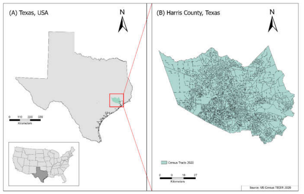
Figure 2.
Analytical workflow used in this study, from data inputs to final outputs. The workflow was drafted by the authors and graphically refined with assistance from ChatGPT (OpenAI).
Figure 2.
Analytical workflow used in this study, from data inputs to final outputs. The workflow was drafted by the authors and graphically refined with assistance from ChatGPT (OpenAI).
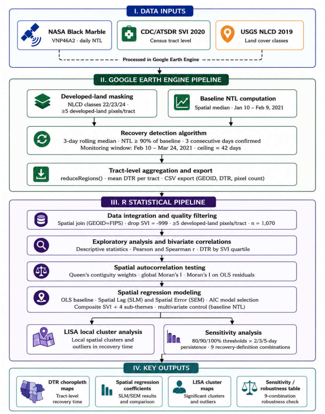
Figure 3.
Spatial distribution of Days to Power Restoration (DTR) across census tracts in Harris County, Texas.
Figure 3.
Spatial distribution of Days to Power Restoration (DTR) across census tracts in Harris County, Texas.
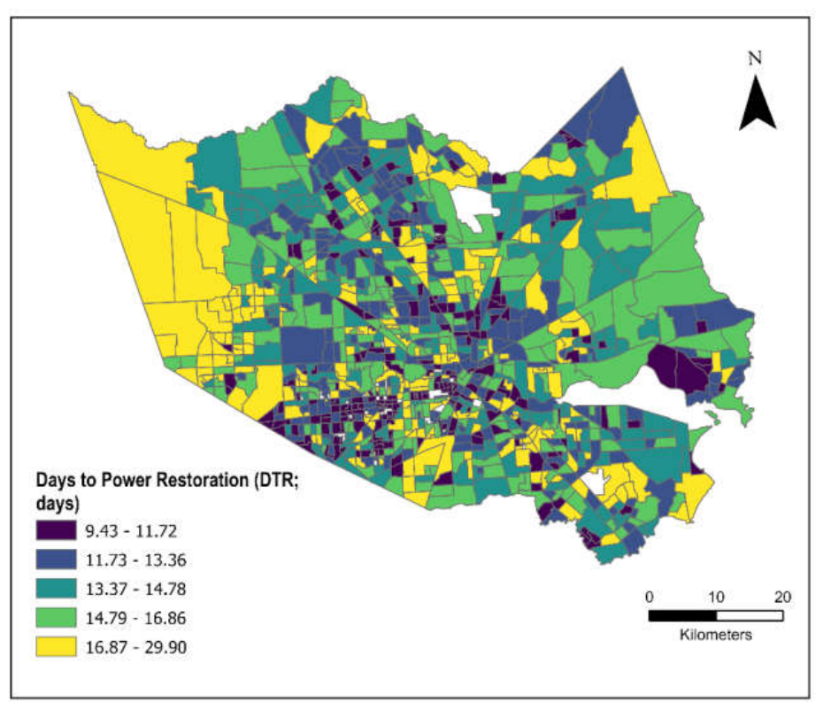
Figure 4.
Spatial distribution of the composite Social Vulnerability Index (SVI) across census tracts in Harris County, Texas.
Figure 4.
Spatial distribution of the composite Social Vulnerability Index (SVI) across census tracts in Harris County, Texas.
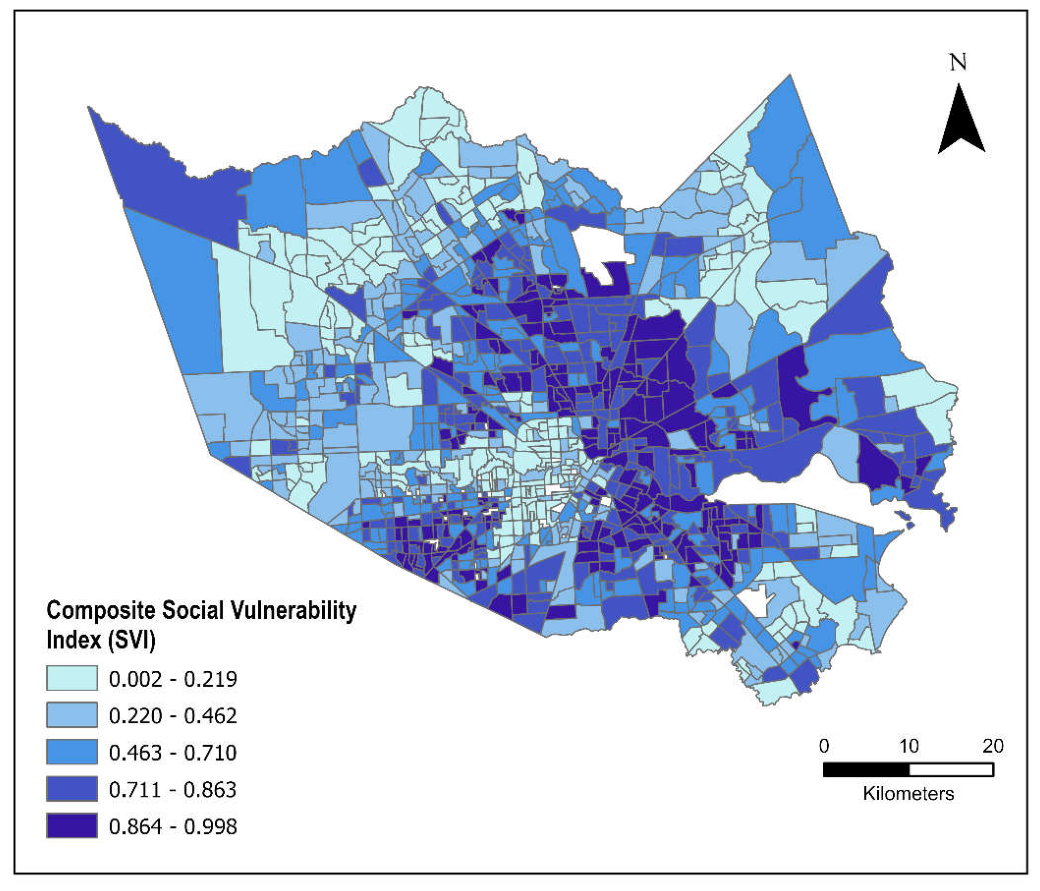
Figure 5.
Relationship between Days to Power Restoration (DTR) and the composite Social Vulnerability Index (SVI) across census tracts in Harris County, Texas. The black line represents the LOESS smoother with the shaded 95% confidence interval, and the red dashed line represents the linear regression fit.
Figure 5.
Relationship between Days to Power Restoration (DTR) and the composite Social Vulnerability Index (SVI) across census tracts in Harris County, Texas. The black line represents the LOESS smoother with the shaded 95% confidence interval, and the red dashed line represents the linear regression fit.
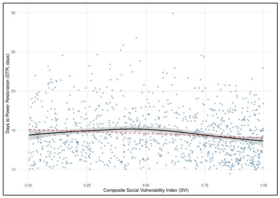
Figure 6.
Moran scatter plot of Days to Power Restoration (DTR), with census tracts colored by Moran quadrant.
Figure 6.
Moran scatter plot of Days to Power Restoration (DTR), with census tracts colored by Moran quadrant.
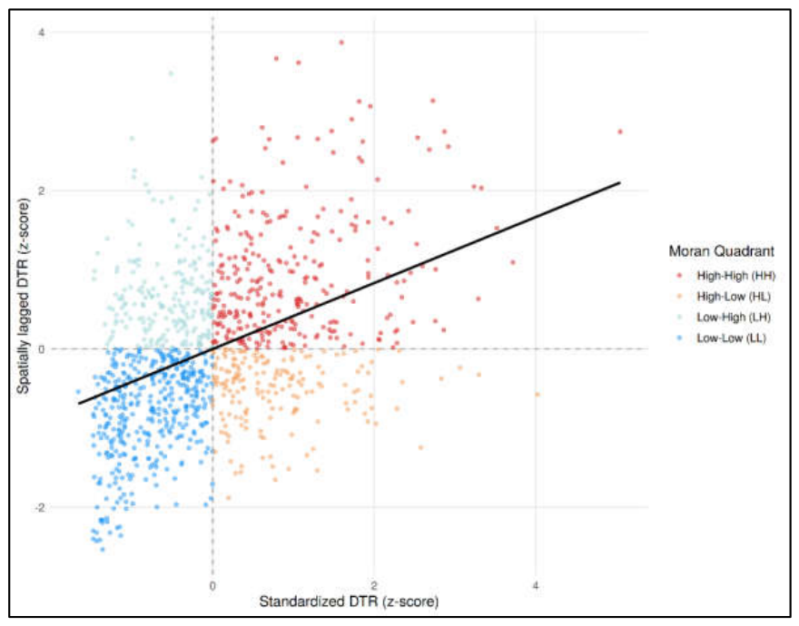
Figure 7.
Spatial Lag Model (SLM) coefficients for the composite Social Vulnerability Index (SVI) and its four themes, with 95% confidence intervals.
Figure 7.
Spatial Lag Model (SLM) coefficients for the composite Social Vulnerability Index (SVI) and its four themes, with 95% confidence intervals.
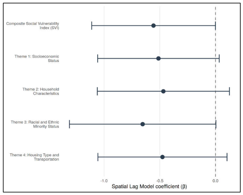
Figure 8.
Relationship between baseline nighttime light (NTL) and the composite Social Vulnerability Index (SVI) across census tracts in Harris County, Texas. The black line represents the LOESS smoother with the shaded 95% confidence interval, and the red dashed line represents the linear regression fit.
Figure 8.
Relationship between baseline nighttime light (NTL) and the composite Social Vulnerability Index (SVI) across census tracts in Harris County, Texas. The black line represents the LOESS smoother with the shaded 95% confidence interval, and the red dashed line represents the linear regression fit.
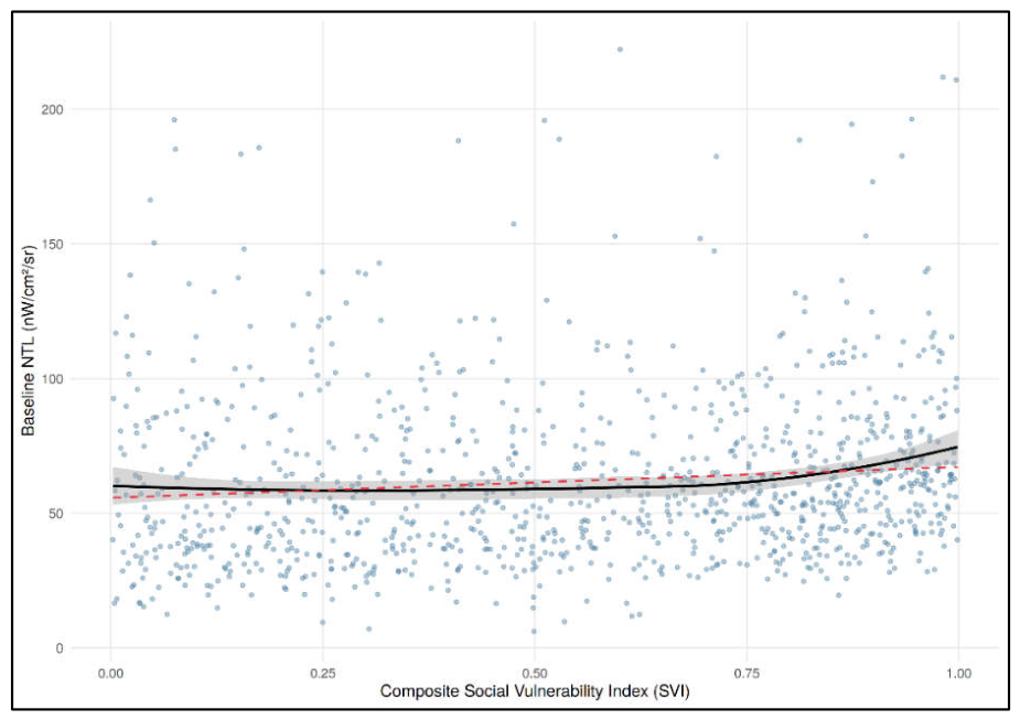
Figure 9.
LISA cluster map of Days to Power Restoration (DTR) across Harris County, Texas. High–High (HH) and Low–Low (LL) indicate significant clusters of high and low DTR; High–Low (HL) and Low–High (LH) indicate spatial outliers (p < 0.05; 999 permutations).
Figure 9.
LISA cluster map of Days to Power Restoration (DTR) across Harris County, Texas. High–High (HH) and Low–Low (LL) indicate significant clusters of high and low DTR; High–Low (HL) and Low–High (LH) indicate spatial outliers (p < 0.05; 999 permutations).
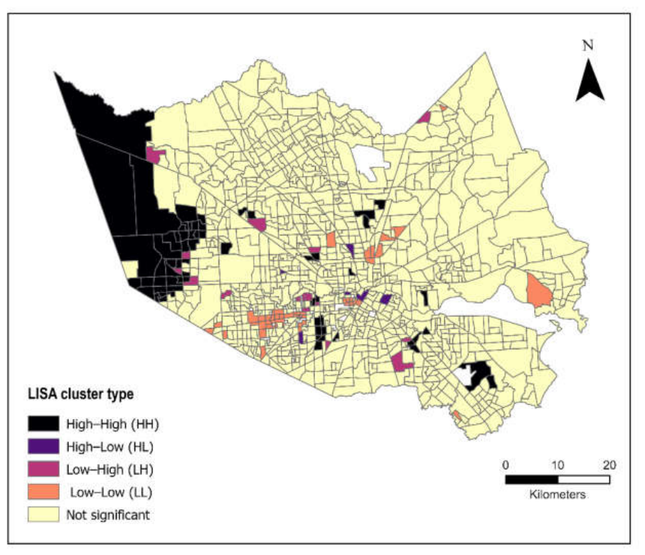
Figure 10.
LISA clusters (a) and composite Social Vulnerability Index (SVI) (b), with High–High (HH; red) and Low–Low (LL; yellow) cluster boundaries overlaid in panel (b).
Figure 10.
LISA clusters (a) and composite Social Vulnerability Index (SVI) (b), with High–High (HH; red) and Low–Low (LL; yellow) cluster boundaries overlaid in panel (b).
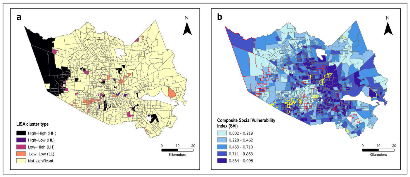

Table 1.
Data sources and characteristics used in this study.
| Dataset | Provider | Resolution | Temporal coverage |
|---|---|---|---|
| NASA Black Marble VNP46A2 | NASA LAADS DAAC | ~500 m | Jan 10–Mar 24, 2021 (daily) |
| CDC/ATSDR SVI 2020 | CDC/ATSDR | Census tract | 2020 (2016–2020 ACS 5-yr) |
| NLCD 2019 | USGS/MRLC | 30 m | 2019 |
| US Census TIGER/Line 2020 | US Census Bureau | Census tract | 2020 boundaries |
ACS = American Community Survey; NLCD = National Land Cover Database; MRLC = Multi-Resolution Land Characteristics Consortium.
Table 2.
Descriptive statistics for Days to Power Restoration (DTR) and CDC Social Vulnerability Index (SVI) measures (n = 1,070 census tracts).
Table 2.
Descriptive statistics for Days to Power Restoration (DTR) and CDC Social Vulnerability Index (SVI) measures (n = 1,070 census tracts).
| Variable | Mean | SD | Median | Min | Max | IQR |
|---|---|---|---|---|---|---|
| Days to Power Restoration (DTR) | 14.51 | 3.05 | 14.06 | 9.44 | 29.90 | 4.06 |
| Composite Social Vulnerability Index (SVI) | 0.551 | 0.305 | 0.580 | 0.003 | 0.998 | 0.554 |
| Theme 1: Socioeconomic Status | 0.580 | 0.310 | 0.640 | 0.002 | 1.000 | 0.562 |
| Theme 2: Household Characteristics | 0.499 | 0.285 | 0.527 | 0.000 | 0.994 | 0.493 |
| Theme 3: Racial & Ethnic Minority Status | 0.641 | 0.258 | 0.696 | 0.012 | 0.989 | 0.436 |
| Theme 4: Housing Type & Transportation | 0.501 | 0.291 | 0.517 | 0.000 | 1.000 | 0.503 |
Table 3.
Days to Power Restoration (DTR) by composite Social Vulnerability Index (SVI) quartile (n = 1,070 census tracts).
Table 3.
Days to Power Restoration (DTR) by composite Social Vulnerability Index (SVI) quartile (n = 1,070 census tracts).
| Composite SVI Quartile | Mean DTR (days) | Median DTR (days) | Standard Deviation | Minimum | Maximum | Mean Composite SVI |
|---|---|---|---|---|---|---|
| Q1 (Least Vulnerable) | 14.55 | 13.82 | 3.10 | 10.02 | 24.57 | 0.136 |
| Q2 | 15.17 | 14.85 | 3.20 | 10.03 | 26.77 | 0.430 |
| Q3 | 14.57 | 14.16 | 2.93 | 10.05 | 29.90 | 0.724 |
| Q4 (Most Vulnerable) | 13.74 | 13.23 | 2.79 | 9.44 | 22.93 | 0.916 |
Table 4.
Pearson and Spearman correlations between Days to Power Restoration (DTR) and Social Vulnerability Index (SVI) measures.
Table 4.
Pearson and Spearman correlations between Days to Power Restoration (DTR) and Social Vulnerability Index (SVI) measures.
| SVI Measure | Pearson r | Pearson p | Spearman ρ | Spearman p |
|---|---|---|---|---|
| Composite Social Vulnerability Index (SVI) | −0.109 | <0.001 | −0.109 | <0.001 |
| Theme 1: Socioeconomic Status | −0.100 | 0.001 | −0.113 | <0.001 |
| Theme 2: Household Characteristics | −0.076 | 0.013 | −0.056 | 0.066 |
| Theme 3: Racial & Ethnic Minority Status | −0.099 | 0.001 | −0.107 | <0.001 |
| Theme 4: Housing Type & Transportation | −0.101 | <0.001 | −0.108 | <0.001 |
Table 5.
Comparison of Spatial Lag Models (SLMs) and Spatial Error Models (SEMs) for Social Vulnerability Index (SVI) measures.
Table 5.
Comparison of Spatial Lag Models (SLMs) and Spatial Error Models (SEMs) for Social Vulnerability Index (SVI) measures.
| Predictor | Model | β | SE | z | p | ρ/λ | AIC | ΔAIC |
|---|---|---|---|---|---|---|---|---|
| Composite Social Vulnerability Index (SVI) | SLM | −0.556 | 0.283 | −1.964 | 0.050 | 0.471 | 5299.4 | −115.6 |
| SEM | −0.478 | 0.384 | −1.245 | 0.213 | 0.473 | 5301.7 | −113.3 | |
| Theme 1: Socioeconomic Status | SLM | −0.512 | 0.278 | −1.839 | 0.066 | 0.473 | 5299.8 | −115.2 |
| SEM | −0.464 | 0.379 | −1.224 | 0.221 | 0.474 | 5301.7 | −113.3 | |
| Theme 2: Household Characteristics | SLM | −0.468 | 0.302 | −1.547 | 0.122 | 0.477 | 5300.8 | −114.2 |
| SEM | −0.435 | 0.377 | −1.153 | 0.249 | 0.478 | 5301.9 | −113.1 | |
| Theme 3: Racial and Ethnic Minority Status | SLM | −0.653 | 0.335 | −1.949 | 0.051 | 0.473 | 5299.4 | −115.6 |
| SEM | −0.911 | 0.501 | −1.818 | 0.069 | 0.473 | 5299.9 | −115.1 | |
| Theme 4: Housing Type and Transportation | SLM | −0.476 | 0.296 | −1.610 | 0.107 | 0.472 | 5300.6 | −114.4 |
| SEM | −0.148 | 0.338 | −0.437 | 0.662 | 0.479 | 5303.0 | −112.0 |
β = regression coefficient; SE = standard error; ρ = spatial lag parameter (SLM); λ = spatial error parameter (SEM); AIC = Akaike information criterion; ΔAIC = difference relative to the OLS baseline (AIC = 5415.0).
Table 6.
Baseline nighttime light (NTL), recovery threshold, and Days to Power Restoration (DTR) by composite Social Vulnerability Index (SVI) quartile.
Table 6.
Baseline nighttime light (NTL), recovery threshold, and Days to Power Restoration (DTR) by composite Social Vulnerability Index (SVI) quartile.
| Composite SVI Quartile | Mean Composite SVI | Mean Baseline NTL (nW/cm²/sr) | NTL Standard Deviation | Recovery Threshold (nW/cm²/sr) | Mean DTR (days) |
|---|---|---|---|---|---|
| Q1 (Least Vulnerable) | 0.136 | 59.42 | 34.67 | 53.48 | 14.55 |
| Q2 | 0.429 | 58.28 | 30.38 | 52.46 | 15.17 |
| Q3 | 0.724 | 61.68 | 28.67 | 55.51 | 14.57 |
| Q4 (Most Vulnerable) | 0.916 | 68.85 | 31.09 | 61.97 | 13.74 |
Recovery threshold = 90% of mean baseline NTL. Sample sizes for Q1–Q4 were 268, 268, 267, and 267 census tracts, respectively.
Table 7.
Multivariate Spatial Lag Model (SLM) results controlling for baseline nighttime light (NTL).
Table 7.
Multivariate Spatial Lag Model (SLM) results controlling for baseline nighttime light (NTL).
| Predictor | SVI Measure | Baseline NTL | Spatial Parameter | AIC | ||||
|---|---|---|---|---|---|---|---|---|
| β | SE | p | β | SE | p | ρ | ||
| Composite Social Vulnerability Index (SVI) | −0.527 | 0.285 | 0.064 | −0.094 | 0.087 | 0.276 | 0.466 | 5300.2 |
| Theme 1: Socioeconomic Status | −0.480 | 0.280 | 0.086 | −0.094 | 0.087 | 0.281 | 0.468 | 5300.7 |
| Theme 2: Household Characteristics | −0.553 | 0.306 | 0.071 | −0.137 | 0.087 | 0.116 | 0.468 | 5300.4 |
| Theme 3: Racial and Ethnic Minority Status | −0.615 | 0.337 | 0.068 | −0.092 | 0.087 | 0.288 | 0.469 | 5300.3 |
| Theme 4: Housing Type and Transportation | −0.402 | 0.309 | 0.193 | −0.077 | 0.090 | 0.395 | 0.470 | 5301.9 |
AIC = Akaike information criterion; ρ = spatial lag parameter.
Table 8.
Days to Power Restoration (DTR) and Social Vulnerability Index (SVI) characteristics by LISA cluster type.
Table 8.
Days to Power Restoration (DTR) and Social Vulnerability Index (SVI) characteristics by LISA cluster type.
| LISA Cluster Type | n | % | Mean DTR | Mean SVI | Theme 1 | Theme 2 | Theme 3 | Theme 4 |
|---|---|---|---|---|---|---|---|---|
| High–High (HH) | 66 | 6.2 | 18.59 | 0.419 | 0.482 | 0.401 | 0.576 | 0.376 |
| Low–Low (LL) | 48 | 4.5 | 11.26 | 0.679 | 0.720 | 0.468 | 0.742 | 0.669 |
| High–Low (HL) | 6 | 0.6 | 16.09 | 0.633 | 0.643 | 0.473 | 0.628 | 0.728 |
| Low–High (LH) | 16 | 1.5 | 12.90 | 0.293 | 0.318 | 0.358 | 0.427 | 0.289 |
| NS (Not Significant) | 934 | 87.3 | 14.40 | 0.558 | 0.584 | 0.510 | 0.644 | 0.504 |
Theme 1 = Socioeconomic Status; Theme 2 = Household Characteristics; Theme 3 = Racial and Ethnic Minority Status; Theme 4 = Housing Type and Transportation. Percentages are based on the full analytical sample (n = 1,070). LISA significance threshold: p < 0.05 (999 permutations).
Table 9.
Composite SVI coefficient from the spatial lag model across alternative recovery-definition thresholds and persistence requirements.
Table 9.
Composite SVI coefficient from the spatial lag model across alternative recovery-definition thresholds and persistence requirements.
| Threshold (%) | Persistence (days) | β | SE | p | ρ | Direction |
|---|---|---|---|---|---|---|
| 80 | 2 | 0.025 | 0.107 | 0.818 | 0.838 | Positive |
| 80 | 3 | -0.027 | 0.184 | 0.882 | 0.524 | Negative |
| 80 | 5 | 1.290 | 0.479 | 0.007 | 0.610 | Positive |
| 90 | 2 | -0.133 | 0.145 | 0.360 | 0.793 | Negative |
| 90 (primary) | 3 (primary) | -0.544 | 0.274 | 0.047 | 0.476 | Negative |
| 90 | 5 | 1.042 | 0.504 | 0.039 | 0.562 | Positive |
| 100 | 2 | -0.347 | 0.213 | 0.104 | 0.746 | Negative |
| 100 | 3 | -1.599 | 0.399 | 0.0001 | 0.466 | Negative |
| 100 | 5 | 0.648 | 0.429 | 0.131 | 0.508 | Positive |
β = SVI coefficient; SE = standard error; ρ = spatial lag parameter. The 90%/3-day row is the primary specification reported elsewhere in this manuscript.
Disclaimer/Publisher’s Note: The statements, opinions and data contained in all publications are solely those of the individual author(s) and contributor(s) and not of MDPI and/or the editor(s). MDPI and/or the editor(s) disclaim responsibility for any injury to people or property resulting from any ideas, methods, instructions or products referred to in the content. |
© 2026 by the authors. Licensee MDPI, Basel, Switzerland. This article is an open access article distributed under the terms and conditions of the Creative Commons Attribution (CC BY) license (http://creativecommons.org/licenses/by/4.0/).
Copyright: This open access article is published under a Creative Commons CC BY 4.0 license, which permit the free download, distribution, and reuse, provided that the author and preprint are cited in any reuse.