
Submitted:
24 August 2026
Posted:
04 September 2026
You are already at the latest version
Abstract
We begin with a simple but uncomfortable question for many firms: if an environmentally
unfriendly company decided to become environmentally performant, what would actually
happen to its turnover? Would sustainability represent merely ’the price of doing good’, or
would it be closer to an investment with a financial return? Should shareholders view it
as a financial risk or as a financial opportunity? To answer these questions, our research
combines a measurable Environmental Performance (EP) index, firm-level data from all
large Romanian companies reporting sustainability measures, and a combination of deep
learning and optimization techniques. We provide evidence that becoming environmentally
performant is less about incurring costs for ethical principles and more about creating
opportunities for improved financial performance. Environmentally unfriendly firms that
would transition toward sustainability would experience a median turnover increase of
3.52%. Moreover, 56.64% of firms would experience a positive effect, with a median gain of
15.61% within this group. For the remaining 43.36%, the median decline of 9.38% is more
appropriately interpreted as a short-term adjustment cost rather than a structural penalty,
consistent with the existing literature.
Keywords:
environmental performance
; sustainability
; turnover
; LSTM
; MILP
; corporate finance
1. Introduction
In the sustainability debate, two broad forces shape the development of policies and research: NGOs and other environment-oriented organizations on one side, and the private market (corporations, firms, investors) on the other. The former primarily seek to limit humanity’s impact on the environment, while the latter are more concerned with the “trade-off of sustainability”, concretely: the price of becoming sustainable. In practice, these two sides often play a never-ending game of shaping, enforcing, or evading policies.
This paper aims to help bridge this gap and contribute to a closer alignment of the two worlds. From the corporate side, preserving the planet is desirable, but financial performance remains the primary objective. Sustainability therefore needs to be framed in a way that is compatible with firms’ financial goals.
The main results presented in this paper are analytic pieces of evidence that, for a company, becoming environmentally performant does not systematically mean to harm financial outcomes and may even create scope for short-term gains, in addition to the long-run positive effects already documented in the literature.
Environmental sustainability is generally understood as managing economic activity in a way that protects key environmental resources and functions over time, and this paper follows that standard definition (Goodland, 1995; UN, 1987).
In this paper, sustainability is made operational through the Environmental Performance indicator, and we follow the standard view that credible sustainability management requires measurable and reportable EP metrics (Epstein & Roy, 2001; Figge et al., 2002; Henri & Journeault, 2008). The relationship between environmental performance and financial outcomes has been widely studied under the “does it pay to be green” question, and the main message from the literature is that the link is usually positive (or at least non-negative), often with effects that show up over time rather than immediately (Albertini, 2013; Friede et al., 2015; Rahi et al., 2023). The definition / construction of the environmental indicators and the outcome-oriented indicators used in this study are taken from Dobre et al. (2025).
We structure our analysis across four areas. We begin by forecasting the Environmental Performance (EP) index using a Long Short-Term Memory (LSTM) neural network, in order to enrich the data set from Dobre et al. (2025). As machine learning models give more accurate estimations when presented with larger data sets this represents an enriching step for our analysis. We then provide an analytic model to classify companies into environmentally performant or not, through a Mixed Integer Linear Programming (MILP) model. Further, we predict turnover using LSTM models, based on historical financial and Environmental Performance data. Finally, we analyze the impact on turnover of becoming environmentally performant.
The paper is organized as follows: Section 2 presents the dataset (596 large Romanian firms, 2019–2024), and summarizes the findings from Dobre et al. (2025) for EP construction, financial variable definitions, and the final five-predictor set used throughout this research. Section 3 introduces the EP forecasting setup, the evaluation metrics, and the dual-input LSTM used to extend EP histories (of three years) for all firms across a full six-year window. Section 4 defines a classification problem and uses a MILP model to select the EP threshold, splitting firms into always-underperforming, always-performant, and switching groups. Section 5 develops the turnover-prediction LSTM trained exclusively on Switching firms, reports its predictive performance, and runs the counterfactual where always-underperforming firms simulate a switch in 2024 to analyze the associated turnover effects.
Overall, the paper presents evidence that becoming environmentally performant is less about paying for one’s principles and more about buying a ticket into a different and, on average, better financial future: at the median, firms that make the switch see a turnover increase of 3.52%, with 56.64% of firms experiencing a positive effect and a median gain of 15.61% within that group. For the remaining 43.36%, the median decline of 9.38% is better interpreted as a short-run adjustment cost rather than a structural penalty.
2. Data Description and Variable Selection
The analysis utilizes a dataset comprising 596 large Romanian firms ( employees). The industry distribution of the companies, according to Dobre et al. (2025), is presented in Table 1. This dataset contains Environmental Performance (EP) scores for the three-year period 2019–2021 with financial and structural data spanning a six-year horizon, 2019–2024.
Environmental Performance (EP) in this study is the score constructed in Dobre et al. (2025), where the authors developed the full methodological framework and applied it to the Romanian firm sample for three consecutive years. For details on the evaluation grid, indicator definitions, weighting scheme, and the coding procedure used to translate sustainability disclosures into a 1–5 EP score, the reader is referred to Dobre et al. (2025). In our work, EP is taken as given and used as the main sustainability signal throughout the forecasting and counterfactual analysis.
The financial statement (cleaned) dataset used in this paper, the full list of raw variables, constructed ratios, and their exact definitions are provided in Dobre et al. (2025). In the present paper, we rely on that dataset and focus on the subset of core predictors identified there: Turnover (T), Total Assets (TA), Solvency Ratio (SOLV), Asset Turnover Ratio (ATR), Firm Age (FA). The authors started from a broad set of financial indicators and after applying correlation screening, regression-based selection, and collinearity diagnostics have arrived at a stable set of core drivers of EP. For the full selection process, statistical tests, and the economic interpretation of each retained predictor, the reader is referred to Dobre et al. (2025). Lastly, Turnover and Total Assets are used in form to reduce skewness and make scales more comparable across firms.
In the present paper, we take this final set as given and use it consistently across all models to keep the analysis comparable. This fixed input set provides a clean and economically meaningful backbone for the EP forecasting, turnover prediction, and counterfactual impact analysis that follow.
3. Environmental Performance (EP) Estimation
This section addresses the first topic of the paper: forecasting firm-level Environmental Performance (EP) for the period 2022-2024.
As presented in Section 2, the dataset contains Environmental Performance scores for the years 2019–2021, and extending EP to the 2022–2024 horizon is essential for the analysis that follows. Forecasting was chosen over direct construction or calculation of EP for two reasons. First, public sustainability data for 2022–2024, needed to construct the EP index is either incomplete or reported on inconsistent scales across firms, which precludes a reliable quantification of environmental performance for those years. Second, and more broadly, forecasting EP rather than recalculating it keeps the framework replicable: because the approach requires only an EP time series and standard firm-level covariates. In this way, researchers working with different EP measures, alternative rating schemes, composite scores, or regulatory-based indicators, can substitute their own data into the same architecture and apply it directly, without redeveloping the variable selection or data collection steps from scratch.
3.1. Error Measurement
Throughout the paper, model performance is assessed using standard error metrics that are widely used in forecasting and machine learning: Mean Squared Error (MSE), Mean Absolute Error (MAE), and Mean Absolute Percentage Error (MAPE).
MSE is used as the training loss for both LSTM models for two reasons. First, by penalizing larger errors disproportionately (Chicco et al., 2021), it is better suited to handle the considerable cross-sectional heterogeneity in firm-level financial data. Second, unlike MAE, MSE is differentiable everywhere, making it compatible with gradient-based optimization via backpropagation.
MAE is used as the primary metric for hyperparameter selection on the validation set. Although the network minimizes MSE during training, MAE provides a more direct and interpretable measure of prediction accuracy in the original units of the target variable, EP on a 1–5 scale and Turnover in absolute terms. Tuning on MAE therefore ensures that the selected hyperparameters yield predictions that are not only well-optimized in a loss sense, but also practically accurate for the firms in the sample.
Lastly, MAPE is reported as a percentage-based complement to MAE, providing a more intuitive view of prediction accuracy relative to the scale of the target variable.
To keep the focus on the modelling and results, we do not discuss forecast evaluation in detail. For formal definitions, properties, and a broader discussion of when each metric is appropriate, the reader is referred to standard forecasting references (e.g. Chicco et al., 2021).
3.2. Long Short-Term Memory Neural Network
Long Short-Term Memory (LSTM) networks are a specific kind of recurrent neural network (RNN) designed to learn patterns from sequence data by addressing the “vanishing gradient” problem that earlier RNNs faced (Bengio et al., 1994; Yu et al., 2019). Here the authors argued that vanishing gradients made it difficult for standard RNNs to capture long-term dependencies, because information from the beginning of a sequence would gradually fade as it was propagated through time. Hochreiter and Schmidhuber (1997) proposed the LSTM architecture as a remedy to this limitation.
The key innovation is the introduction of a memory cell equipped with gates that regulate information flow. Intuitively, these gates act like valves: a forget gate determines how much of the past to retain, an input gate controls which new information is written into the cell state, and an output gate decides how much of the internal memory is exposed to produce the current output (Hochreiter & Schmidhuber, 1997). By training these gating functions, LSTMs can retain information over longer horizons while still reacting to short-term patterns (Gers et al., 2000).
This architecture creates two distinct information pathways: one for long-term context (the cell state) and one for shorter-term signals (the hidden state). Along the cell-state path, information from earlier in the sequence can pass forward largely unchanged, rather than being repeatedly scaled by small weights as in a standard RNN, thereby preserving long-range dependencies (Hochreiter & Schmidhuber, 1997).
This structure is particularly useful in firm-level settings, where both persistence (e.g. structural characteristics) and short-term variation (e.g. recent financial changes) play a role. By dynamically filtering information over time, the LSTM can capture these effects without imposing a fixed functional form on how past observations influence current outcomes.
Beyond their architectural properties, LSTMs have emerged as one of the most successful tools for prediction tasks in financial markets, a domain whose noise, non-stationarity, and complex non-linear dependencies have outperformed the precision of traditional statistical models (J. Qiu et al., 2020). In a large-scale application to all S&P 500 constituents from 1992 to 2015, (Fischer & Krauss, 2018) show that LSTM networks outperform random forests, standard deep neural networks, and logistic regression in both predictive accuracy and risk-adjusted returns. Comparable evidence is reported across markets, prediction targets, and benchmarks. Y. Liu (2019) finds that LSTMs serve as a robust non-linear regression for S&P 500 and AAPL volatility forecasting in cases where Support Vector Regression underperforms, while Budiharto (2021) shows that LSTMs dominate ARIMA on Indonesian stock-price data by exploiting non-linear dynamics that linear time-series models cannot capture. The same properties have motivated several extensions tailored to financial series: Bao et al. (2017) combine wavelet transforms, stacked autoencoders, and LSTM to forecast six major stock indices, while J. Qiu et al. (2020) augment an LSTM with an attention mechanism on the S&P 500, DJIA, and Hang Seng indices, both reporting statistically significant gains over conventional benchmarks. On the application side, Ta et al. (2020) integrate an LSTM stock-price forecaster into a quantitative portfolio strategy that outperforms the S&P 500 in both active return and Sharpe ratio. Taken together, these results justify the choice of an LSTM architecture for the EP forecasting task developed in this paper, where firm-level Environmental Performance and especially company turnover exhibit the same noisy and non-linear dynamics that have driven LSTMs’ success in financial-market applications.
For the technical and mathematical aspects of the LSTM architecture, the reader is referenced to the work of Hochreiter and Schmidhuber (1997), Gers et al. (2000), Bengio et al. (1994), Yu et al. (2019).
Both models, the EP prediction model and the Turnover prediction model, follow the same dual-input structure. Each consists of two branches: an LSTM branch that captures historical dynamics and a Dense branch that incorporates current-year information. The exact inputs and configurations differ across the two models and are discussed separately. What is common to both is the training–validation–testing framework.
We will define here the parameters governing the mechanisms of the LSTM, namely the weight matrices and and biases which are learned directly from the data during training. After defining the architecture, an initial set of hyperparameters is chosen based on standard practice and existing literature in similar forecasting settings, both of which are detailed in the model-specific subsections that follow. This serves as a starting point rather than a final specification.
Hyperparameter tuning is then performed, which is a critical step in the model development process. The hyperparameters considered are the number of LSTM units, the number of Dense units, the learning rate, and the batch size. For each hyperparameter, a grid search is conducted: the model is retrained across a predefined set of candidate values, and performance is evaluated using the validation MAE.
Concretely, for a parameter such as the number of LSTM units, the model is first trained with a low value (e.g. 4 units), the validation MAE is recorded, and the process is repeated for increasing values (e.g. 8, 16, 32, etc.). After evaluating all configurations in the grid, the value that yields the lowest validation MAE is selected and fixed. This procedure is applied sequentially to each hyperparameter, with previously selected values carried forward.
The rationale behind each grid and the final selected values are discussed in the following section.
3.3. Dual-Input LSTM Network for EP Prediction
The model is designed to predict i-th firm’s Environmental Performance (EP) score for a target year t, where the score is a numeric rating bounded between 1 (lowest) and 5 (highest). It combines two complementary sources of input: a historical sequence of past data and the firm’s current-year financial features, allowing the model to ground its predictions in learned temporal patterns while remaining responsive to the firm’s current financial conditions.
The historical input branch processes a sequence of length L consisting of the firm’s EP scores from previous years (2019–2021 in the training setup) together with its financials: solvency (SOLV), firm age (FA), , asset turnover ratio (ATR), and . This sequential information is passed through a Long Short-Term Memory (LSTM) layer with 32 units, which captures temporal dependencies, trends and patterns across years, and outputs a hidden state vector summarizing the firm’s recent history.
In parallel, the current-year branch takes the firm’s current financial indicators for the prediction year (for example, 2022), using the same transformation for total assets and turnover, and passes them through a dense layer with 16 neurons. This branch captures cross-sectional information that is specific to the prediction year and not dependent on past dynamics.
The outputs of the two branches are concatenated into a joint representation that integrates both temporal patterns and current firm conditions.
The concatenated representation is then passed through a fully connected output layer (a dense neural network layer). This output layer produces a single numeric prediction , for firm i in year t. Because EP is defined on a 1–5 scale, the model uses a scaled sigmoid activation.
The dual-input LSTM model is trained on historical data of firms’ EP scores and features, to minimize the prediction error. Formally, if is the actual observed EP of firm i in year t, the training objective is to minimize the mean squared error (MSE) between the predictions and actual values across all training examples:
where the sum is over all firm-year instances in the training set.
The model’s parameters, including the LSTM weights and the output layer weights, are optimized to minimize this loss. The model was implemented in Python using TensorFlow and its high-level Keras API for the construction, training, and evaluation of the LSTM network. Data preprocessing was carried out with pandas and numpy, while scikit-learn was used for feature scaling via StandardScaler and for firm-level train–validation–test splits. Visualizations were generated using matplotlib. The development environment was Spyder, part of the Anaconda distribution. Experiments were conducted on a MacBook Pro with an Apple M3 Max chip.
An approximate 70/15/15 firm–level train–validation-testing split was employed, resulting in 416 training firms, 90 validation firms, and 90 testing firms.
Before training, inputs in each branch were standardized with StandardScaler (zero mean, unit variance) to put variables on a comparable scale and support stable, fast optimization.
To train the dual-input LSTM network for predicting environmental performance (EP) scores, several hyperparameters were tuned. They were chosen based on the performance of the model on the validation set.
3.4. Baseline Configuration
The sequence length () determines how many past time steps (lags) the LSTM uses as input. In this model, the network looks back two periods (2019 and 2020) to approximate the next EP score in 2021. Choosing the lag length involves a trade-off between capturing temporal dependence and keeping the model parsimonious. In standard econometric settings, the lag order is typically kept low unless the data clearly suggest a longer memory. Recurrent architectures such as LSTMs, however, handle temporal dependencies internally, so the exact number of input lags is less critical than in static models. Because the LSTM’s internal state can, in principle, retain information over longer horizons, a relatively short input window is sufficient. The allows the model to be trained on 2019 and 2020 and used to predict 2021.
The number of units in the LSTM hidden layer is selected through a grid search in the range of 4 to 64 (4, 8, 16, 32, 64), using the baseline configuration for the remaining hyperparameters. This choice is motivated by the literature, which treats the number of hidden units as a key hyperparameter that must balance model capacity and generalization. Existing studies typically explore broad intervals rather than fixed values, with ranges such as 16 to 100 units (Cortez et al., 2018) and 4 to 128 units (Abbasimehr et al., 2020; Chang et al., 2022; L. Liu et al., 2022).
Importantly, it is well established that too few units limit the model’s ability to capture temporal dependencies, while too many introduce unnecessary complexity and may harm performance by modelling noise(L. Liu et al., 2022). In this context, the interval of 4 to 64 units provides a focused yet representative search space, capturing both low-capacity and moderately complex architectures, and is subsequently explored through grid search.
The number of neurons in the Dense layer (capturing current-year financial variables) follows the same literature-backed grid search strategy, with a small adaptation to reflect its role within the model. Specifically, the grid search interval mirrors that of the LSTM layer, but all values are carefully monitored and scaled down by a factor of two. This monitoring and adjustment is motivated by two considerations. First, an excessively small Dense layer relative to the LSTM component would reduce its contribution after concatenation, limiting the influence of contemporaneous financial information in the final prediction. Second, given the expectation that current-year variables contain relevant predictive signals, this scaled grid allows for a formal test of whether architectures that preserve this balance indeed achieve superior validation performance, as measured by validation MAE. The grid search is performed combinatorially across the values of the two layers, with the model trained iteratively for each possible combination of hyperparameters.
An initial learning rate of 0.01 is adopted as the baseline configuration. This choice is supported by evidence in the literature indicating that effective learning rates are not fixed, but lie within a range that balances convergence speed and training stability. Most commonly, studies consider values in the interval 0.001–0.01 (Budiarso, 2024; L. Liu et al., 2022; K. Qiu et al., 2022), while some extend the search to wider ranges, exploring values as low as 0.0001 and as high as 0.1 or even 0.3 (Jiang & Xu, 2022; L. Liu et al., 2022; Smith, 2018). Complementing this, Martyushev et al. (2025) treat the learning rate explicitly as a hyperparameter to be tuned via cross-validation, reinforcing the idea that no universally optimal value exists and that systematic search over a predefined interval is required.
The Adam optimizer literature (Kingma & Lei Ba, 2015) recommends a default learning rate of , which serves as a widely accepted benchmark in practice. While this recommendation informs the design of the validation grid search, an educated choice is made to adopt a higher initial value of 0.01 for the baseline model, allowing faster initial convergence and positioning the model within the empirically effective range identified in prior work. Taking these considerations together, the grid search is conducted over , covering the most commonly cited interval as well as the Adam default and broader values explored in the literature.
A batch size of 32 is used as the baseline configuration. This choice follows standard practice in deep learning, where stochastic gradient methods are typically run with batches in the range of 32–256, balancing computational efficiency with statistical noise in the gradient estimate (Fan et al., 2021; Goodfellow et al., 2016). Empirical work on batch-size effects shows that very large batches tend to converge to local minima and suffer a generalization gap compared to small-batch training (Keskar et al., 2016), while systematic experiments across CIFAR-10, CIFAR-100 and ImageNet report that the best test performance and training stability are consistently obtained for mini-batch sizes between 2 and 32 (Masters & Luschi, 2018). Building on this, a grid search over batch sizes ranging from 8 to 128 is conducted to empirically assess the trade-off between gradient noise and convergence stability, following common experimental setups in the literature (Fan et al., 2021; Goodfellow et al., 2016; L. Liu et al., 2022; Masters & Luschi, 2018). This allows the initial choice of 32 to be validated against both smaller and larger batch regimes. Taking these considerations together, the grid search is conducted over , spanning the small-batch regime favored by the empirical generalization literature and the larger sizes recommended for computational efficiency.
Table 2 shows the results of the LSTM-Dense neurons grid search.
The lowest validation MAE is obtained for the configuration, with a value of . Although other structures attain a slightly lower validation MSE, they also exhibit a marginally higher validation MAE than .
The grid search over learning rates selected , which achieved the lowest validation MSE and MAE (Table 3).
The grid search over batch sizes selected 32, which achieved the lowest validation MSE and MAE (Table 4).
The learning-rate scheduler also operated as intended. The model started with a relatively high learning rate (0.01), which enabled rapid progress during the initial epochs. As shown in Figure 1, once the validation error stopped improving, the scheduler progressively reduced the learning rate in steps, allowing the optimizer to become more cautious and to fine-tune the weights. In combination with early stopping at epoch 42 (well below the 200-epoch upper bound set as a safeguard), this ensured that training halted near the point of best generalization, avoiding both unnecessary additional epochs and drift into overfitting.
The final hyperparameter configuration of the dual-input LSTM, selected through the sequential grid searches described above, is summarized in Table 5. This specification is used in all subsequent training, evaluation, and forecasting steps.
The final performance of the dual-input LSTM after hyperparameter tuning on the validation set (90 companies) is presented in Table 6.
3.5. EP Prediction Results
After training and validation the model is evaluated on the test set, comprising the remaining 90 companies that have not been used at any prior stages. This will tell us whether the selected hyperparameters can generalize across companies and if there is a bias towards the validation set.
As shown in Table 6, the test MSE (MSE = 0.0096) is slightly higher than the training MSE (MSE = 0.0051), as is expected when evaluating on unseen data. The same pattern holds for the MAE, where the gap between the two sets remains small, indicating that the model generalizes well to companies not seen during training or hyperparameter tuning.
The final evaluation approach analyses the model’s approximations of EP in 2021, obtained after training on 2019–2020 data, for all firms in the dataset. In this configuration, the mean absolute error (MAE) across all firms for 2021 is , indicating that the dual-input LSTM maintains good accuracy when forecasting one year ahead using only past information. Furthermore, a deviation of between the historical and predicted EP values is almost negligible on the 1–5 Environmental Performance scale, further reinforcing the model’s practical reliability.
Further, using this model predictions are made to obtain the EP employed in the next sections, which examines the relationship between Environmental Performance and financial outcomes. The resulting dataset contains 593 (3 firms dropped due to corrupted data) firms with Environmental Performance values for six consecutive years (2019–2024), accompanied by their corresponding financial indicators.
4. Classifying Environmental Performance Using Prescriptive Analytics
This section introduces a classification framework that splits firms into environmentally underperforming (coded as 0) and environmentally performant (coded as 1), and defines a third group of interest: Switching firms that move from low (code 0) to high EP (code 1) at least once over the 2019–2024 period. A Mixed Interger Linear Optimization (MILP) model is used to select a threshold on the EP scale that maximizes the number of such meaningful switches (thereby creating a sufficiently large dataset for training the subsequent LSTM model) while remaining consistent with common practice in the EP literature.
4.1. Threshold Formulation via Mixed Integer Linear Programming
To identify an appropriate threshold for this classification, two aspects must be balanced: maximizing the number of firms that exhibit a transition from underperforming to performant status across the period, and ensuring consistency with thresholds commonly referenced in the academic and industry literature on environmental performance measurement. In essence, the goal is to determine a threshold, empirically justified and theoretically supported, that produces the greatest number of meaningful switches. These transitions provide valuable insights into the potential financial changes associated with firms becoming environmentally performant.
Mixed Integer Linear Programming (MILP)
We define by the threshold we need to compute. Each firm i is characterized by its minimum and maximum value for the Environmental Performance (EP) across the six-year horizon (either observed or predicted) . Table 7 summarizes the notation used for our model.
Decision Variables.
- : the EP threshold to be selected.
- : binary variable indicating that firm i can strictly cross the threshold at some point in time, starting from a lower EP level (switching firm).
MILP Formulation.
Our proposed MILP is defined as follows:
The objective (1) maximizes the number of firms classified as switching. When , constraints (2)–(3) reduce to
so the threshold lies strictly above the firm’s minimal EP and no higher than its maximal EP.
When , the M values relax the bounds back to , so firm i does not restrict the feasible region. The global bounds (4) reproduce the observed EP range, and (5) enforces the binary nature of .
Interpretation.
At the optimal solution , we have
Thus, equals the maximum number of firms for which there exists a single global threshold that lies strictly above their initial EP level but no higher than their final EP level on 2019–2024. These firms are classified as transitioning from environmentally underperforming to environmentally performant over the observation window ("Switching firms").
It is important not to mistake the codes 0 and 1 for the performance of a company with the possible values of the decision variable , where will characterize a firm as switching and as non-switching.
4.2. Results
The MILP is solved in Python using gurobipy, with data handling via pandas/numpy. The script ingests the panel from xlsx, computes firm-level EP ranges , builds a model with a small strictly-improving offset on the lower bound, solves for the optimal threshold , and then exports firm-level upgrade labels .
The MILP identified a unique threshold of , which maximizes the number of firms whose EP values cross the threshold at least once over 2019–2024. At , the model identifies 370 Switching firms out of 593 total (). Among all firms, 59 remain consistently environmentally performant (all EP values above the threshold), while 164 remain consistently underperforming (all EP values below the threshold). These three groups provide a clear and interpretable categorization of firms’ environmental profiles based on their EP trajectories. A summary of the MILP outcome is presented in Table 8.
Due to the lack of consensus in the literature and methodology concerning the quantification of an environmental performance index, multiple academic and industry frameworks utilize proportional or percentile-based methods for classifying firms and identifying those that are leading or lagging. For instance, MSCI (2024) calculates percentile and quartile distributions of ESG scores among industry peer groups to establish performance categories, whereas the London Stock Exchange Group (LSEG, 2024) ranks companies through percentile transformation to normalize the distribution of ESG scores. Moreover, the ISS ESG rating methodology categorizes “Prime” organizations as those positioned above the 50th percentile within their respective industry (ISSESG, 2021).
Our MILP provides a quantitative way of implementing the percentile-based rule supported by the literature, directly on the EP panel.
The optimal threshold , which categorizes about of the firm-year data as environmentally performant (labeled as 1), reflects a median-oriented methodology. This aligns with the utilization of median or higher-quartile allocations, as previously described, rather than absolute indices.
Ehlers et al. (2022) emphasize that quartile-based screening efficiently distinguishes sustainability leaders while ensuring comparability among enterprises with varying reporting intensity.
It is important to highlight that, due to the lack of general consensus in the literature on the precise quartile that objectively characterizes environmental performance, should be regarded as context-specific rather than a universal standard. The non-comparability among research studies is emphasized by Berg et al. (2022), who demonstrate an average correlation of only between the empirical investigations of ESG rating agencies. Nonetheless, the threshold established in this paper offers a coherent and transparent classification within the dataset.
Figure 2 shows the distribution of Environmental Performance (EP) values along with the chosen threshold. The distribution exhibits a slightly left-skewed Gaussian shape, with the majority of EP values concentrated between 3 and . This pattern further supports the selected threshold, indicating that it is representative with respect to the overall dataset.
Taken together, the results show that the proposed MILP-based approach successfully identifies a sustainability threshold that categorizes firms into underperforming, switching and consistently performant groups.
5. Assessing Sustainability’s Financial Payoff
This section labels firms based on their EP values and presents a Long Short-Term Memory (LSTM) Neural Network model that predicts turnover using financial trajectories and sustainability labels. After evaluating the model’s predictive performance, the analysis turns to the main goal: using a trained LSTM to simulate how the turnover of always-underperforming firms would change if they became environmentally performant. The resulting distribution of effects provides the core quantitative answer to the question of how changing EP is reflected in firms’ turnover.
5.1. Dual-Input LSTM Network for Turnover Prediction
The network design follows the same conceptual structure as the model previously applied for Environmental Performance (EP) forecasting, with a few adjustments.
Firstly, while the EP prediction LSTM used the original EP score (1-5) as the dependent variable, the present model employs the binary EP label defined in Section 4.2 as predictor. Concretely, each firm–year observation with an EP score at or above the sustainability threshold () is labeled as 1, and those below the threshold as 0. This coding makes it possible to identify the year in which a company becomes environmentally performant (EP label switches from 0 to 1) and allows the model to learn from this discrete transition.
The model uses two input systems as well. The first one, called the history branch, utilizes a sequential input of length 5 (five consecutive years) and has the six features described in Section 2: label, , , , , and . This branch passes through an LSTM layer with 8 units, which captures temporal dependencies and firm-specific evolution patterns across time.
The second one, called the current-year branch, contains the EP label of a company in the current year. It is passed through a Dense layer with 4 neurons and ReLU activation. This component captures the direct, nonlinear impact of current sustainability conditions on financial outcomes. The outputs of the two branches are concatenated and passed to a final output layer, which produces the network’s prediction . To retrieve the predicted value in natural units, the inverse transformation:
is applied.
The dual-input LSTM model uses information from the years 2019–2023 to predict each company’s Turnover in 2024 and is trained to minimize the Mean Squared Error (MSE). The rationale behind the choice of the MSE metric was discussed in Section 3.1, as well as the corresponding loss (MSE) function.
Out of the 593 firms, 27 were dropped (16 from the switching sample and 11 from the always underperforming one) because they exhibited drastic changes in Turnover in 2024 (e.g., declines of 50% to 95%), likely due to firm-specific issues, or reported Turnover equal to 0.
The dual-input LSTM is trained exclusively on the 354 Switching firms, i.e., those that, within the six-year sample window, start from not being environmentally performant and subsequently cross the sustainability threshold discussed in Section 4.2.
The rationale for training exclusively on these firms is that the analysis aims to understand how a firm’s financials respond when it becomes environmentally performant. Restricting the training set to companies that actually undergo this transition focuses the model on the relevant regime, increasing the likelihood of capturing complex non-linear relationships associated with EP upgrades and improving the efficiency of the learning process.
The always-underperforming firms will be used later to evaluate the impact on Turnover if they were to become performant in 2024.
An 70/15/15 train–validation-test split was employed. The division can be visualized in Figure 3.
As with the first LSTM, the model is trained on the training pool, hyperparameters are tuned by minimizing the validation MAE, and final performance is evaluated on the held-out test set. This ensures that the selected hyperparameters are not biased towards any specific subset of firms, thereby avoiding overfitting and confirming that both the results and the methodology generalize to unseen companies.
The sequence length L determines how many past time steps (lags) the LSTM uses as input. Since the augmented dataset now contains six consecutive years, it is possible to choose a larger sequence length. Setting allows the model to be trained on years 2019–2023 and used to approximate, and subsequently predict, Turnover in 2024.
Before training, all input features in both branches were standardized using StandardScaler. The scalers were fitted on the training data and then applied to the validation inputs, so that each training feature has approximately mean zero and unit variance. Such normalization is standard in neural network applications, as it places all inputs on a comparable scale, prevents large-magnitude variables from dominating the optimization, and typically improves the stability and speed of convergence during training.
The number of neurons in the LSTM and Dense branches is selected via a grid search following the same scaled-dense rationale described in Section 3.4, to which the reader is referred for the full justification and supporting literature. The motivation is, if anything, stronger here: the Dense branch carries the current-year EP label, the variable whose effect on turnover is the central object of interest, so its capacity must remain large enough relative to the LSTM branch to preserve its contribution at concatenation. The LSTM grid is therefore explored over and the Dense grid over , with the smallest configurations tested in the EP model ( for the LSTM branch and for the Dense branch) excluded here. The turnover-prediction task is structurally more involved, since the model must learn the joint dynamics of financial trajectories and a binary EP signal rather than approximate a single bounded score, and configurations with such limited capacity cannot reasonably be expected to capture the relevant non-linear interactions.
The learning rate is tuned following the same procedure and over the same grid as in Section 3.4, to which the reader is referred for the full motivation and supporting literature. The baseline value, however, is set to rather than . The rationale is twofold: the architecture here is more involved, since it carries a binary EP label through the Dense branch on top of the historical sequence, and the training sample is smaller, as the model is fitted exclusively on Switching firms. A more conservative starting rate reduces the risk of unstable updates in this lower-data, higher-complexity regime, while the grid search ensures that the full interval is still explored. As an additional safeguard, the smallest value documented in the literature review of Section 3.4, , is also included in the grid.
The batch size is tuned following the same procedure and over the same grid as in Section 3.4, to which the reader is referred for the full motivation and supporting literature. The baseline value, however, is set to rather than . With fewer firms in the training set, smaller batches provide more frequent gradient updates per epoch, which helps stabilize learning when data is limited, while the grid search ensures that larger regimes up to are still explored.
Number of Neurons in LSTM and Dense Branches
The lowest validation MAE is obtained for the configuration, with a value of . Although the other structures attain a slightly lower validation MSE, they also exhibits a marginally higher validation MAE than .

Table 9.
LSTM Grid Search Results.
| LSTM | DENSE | Train MSE | Validation MSE | Train MAE | Validation MAE |
|---|---|---|---|---|---|
| 8 | 4 | 0.032652 | 0.025036 | 0.134060 | 0.120809 |
| 8 | 8 | 0.030136 | 0.024420 | 0.127379 | 0.123975 |
| 8 | 16 | 0.032557 | 0.035536 | 0.134982 | 0.140323 |
| 8 | 32 | 0.031535 | 0.025859 | 0.131694 | 0.122283 |
| 16 | 4 | 0.029915 | 0.025655 | 0.129664 | 0.128142 |
| 16 | 8 | 0.028895 | 0.024946 | 0.128837 | 0.127199 |
| 16 | 16 | 0.031392 | 0.030282 | 0.133607 | 0.141612 |
| 16 | 32 | 0.031926 | 0.032219 | 0.136168 | 0.137356 |
| 32 | 4 | 0.030049 | 0.035811 | 0.133296 | 0.150788 |
| 32 | 8 | 0.030634 | 0.026562 | 0.133271 | 0.132643 |
| 32 | 16 | 0.025024 | 0.034206 | 0.117452 | 0.137814 |
| 32 | 32 | 0.031090 | 0.024276 | 0.132692 | 0.127275 |
| 64 | 4 | 0.024580 | 0.033105 | 0.121093 | 0.126592 |
| 64 | 8 | 0.023955 | 0.048120 | 0.116762 | 0.153140 |
| 64 | 16 | 0.032189 | 0.036628 | 0.135905 | 0.138851 |
| 64 | 32 | 0.016667 | 0.056664 | 0.096450 | 0.140790 |
The table reports training and validation performance for each LSTM–Dense layer configuration. The shaded row represents the best-performing model based on validation MAE. MSE denotes the mean squared error, while MAE denotes mean absolute error.
Learning Rate
To select an appropriate value, a grid search over was can be seen in Table 10.
The learning-rate grid search indicates that yields the lowest validation MAE () and validation MSE (). Since outperforms the baseline of chosen above, it is adopted as the final learning rate of the model and carried forward into the batch-size grid search.
Batch Size
The grid search over batch sizes can be seen in Table 11.
Among the tested configurations, achieves the lowest validation MAE as well as MSE, while requiring the only 277 epochs.
L2 Regularization
L2 regularization was not explored for the EP prediction LSTM, as its low errors and small training–validation gap indicated no material overfitting. For the turnover-prediction model, however, this concern is more realistic: the target is firm-level turnover rather than a bounded 1–5 score, and the training sample, restricted to Switching firms, is considerably smaller.
L2 regularization is commonly used in LSTM models to reduce overfitting by penalizing large network weights and controlling their norm (Merity et al., 2017; Pacella et al., 2024). This is particularly relevant for firm-level financial data, where variables differ widely in scale and volatility and are often correlated, which increases the risk that the model fits firm-specific noise. In practice, L2 regularization tends to improve out-of-sample performance by reducing the training–validation gap, and it is typically tuned via a grid search over penalty values to minimize validation error (Abbasimehr et al., 2020; Borovkova & Tsiamas, 2019; Harvey et al., 2024; Kang et al., 2024; Kaushik et al., 2020).
Given the dual-branch architecture, L2 regularization was applied to multiple components: the LSTM layer (kernel, recurrent and bias terms), the current-year dense layer (kernel), and the output layer (kernel). The regularization strength was selected via a small grid search over , allowing the model to balance flexibility and generalization without introducing unnecessary complexity.
Among the tested values, the L2 rate delivers the lowest validation MAE and MSE (Table 12), indicating that the model does not materially benefit from L2 regularization. For this reason, the final model is estimated without L2 regularization.
The maximum number of epochs was set to 500 to allow sufficient training time, if required. In practice, training typically terminates earlier via early stopping: when the validation MAE does not improve for 70 consecutive epochs (patience ), training is halted and the best-performing weights are restored to mitigate overfitting.
In addition, a learning-rate schedule is applied using ReduceLROnPlateau (patience , factor ). If the validation MAE fails to improve for 20 epochs, the learning rate is multiplied by . The underlying idea is to start with a relatively high learning rate to enable rapid progress in the initial epochs and then progressively reduce it once improvements slow down, allowing for more precise convergence around local minima.
These settings were closely monitored and iteratively refined during hyperparameter tuning by inspecting the MAE, MSE and learning-rate trajectories. The final configuration achieves the best validation performance while maintaining low volatility across training and validation curves.
The final hyperparameter configuration of the dual-input LSTM for turnover prediction, selected through the sequential grid searches described above, is summarized in Table 13. This specification is used in all subsequent training, evaluation, and counterfactual analyses.
To assess the model’s validity and performance, the final training and validation error metrics were examined alongside the learning curves, in order to verify that the network learns in a stable manner and does not exhibit persistent divergence.
Performance
Table 14 summarizes the final performance metrics of the model. Both MSE and MAE are low, with only a small gap between the training and validation sets. The model attains a MAPE of on the training set and on the validation set, a difference of just percentage points. This indicates good generalization and confirms the model’s stable predictive performance.
5.2. Turnover Prediction Results
This subsection directly addresses the question of predicting a firm’s turnover from its historical financials and EP status using a Long Short-Term Memory (LSTM) network.
Now that the model has been trained on the training set and the hyperparameters tuned to minimize the validation MAE, the final evaluation is conducted on the held-out test set, comprising the 54 firms not used at any prior stage. This provides an unbiased estimate of the model’s predictive accuracy and, more importantly, its ability to generalise to unseen companies. Table 15 shows the out-of-sample results .
As shown in the table, the distribution of the absolute percentage error on the test set is mildly right-skewed, the mean (15.18%) lying between the median (10.22%) and the 75th percentile (18.82%). This indicates that while the majority of the model’s approximations show low error (as confirmed by the low median), the mean is slightly pulled upward by a small number of volatile cases or outliers.
Overall, the predictive performance remains robust and reliable, demonstrating that the proposed dual-input LSTM network successfully forecasts firm-level turnover with relatively low out-of-sample error from recent financial history and the EP label.
5.3. Environmental Performance Influence on Turnover
After establishing validity, performance and generalization, the dual-input LSTM is used to examine the main topic of this paper. In the previous section, 153 firms were classified as “always environmentally underperforming”, meaning that they remained below the sustainability threshold in every year from 2019 to 2024.
Our model is now applied in a counterfactual manner to these firms, predicting their 2024 turnover under the assumption that they had become environmentally performant in 2024.
Concretely, the EP label feeding the current-year (Dense) branch is set to 1 for 2024, while all other inputs are kept unchanged, and the network produces a counterfactual 2024 turnover. This setup provides an estimate of the turnover change associated with attaining environmental performance, ceteris paribus.
Figure 4 shows the distribution of absolute differences between the actual 2024 turnover of always–underperforming firms and the turnover predicted under the assumption that the firm became environmentally performant in 2024. As it can be seen, approximately of changes lie within the interval , with a smooth distribution around zero and a small number of left and right-tail outliers. This pattern supports the interpretation that the central tendency reflects modest positive effects on average, while rare idiosyncratic events can still generate large deviations.
It should be noted that this is purely an analysis of change effects, intended to summarize the overall magnitude of the switch effect. A more detailed examination of positive versus negative impacts follows in the next subsection.
This section directly addresses the effect on a firm’s turnover of becoming environmentally performant by quantifying the predicted percentage change in turnover when firms switch from environmentally underperforming to environmentally performant status. To further analyze the predicted financial impact, the amplitude-of-change analysis focuses on the approximately of firms within the main range of effects, excluding the ten outliers that can be seen in Figure 4 such that the results are not driven by these exceptional cases.
Of the 143 companies, 81 (56.64%) experienced a positive effect and 62 (43.36%) a negative one. A summary of the results is shown in Table 16. The distribution of percentage differences in turnover (Table 16) is clearly skewed and heavy–tailed, with a small number of firms experiencing very large positive or negative changes after becoming environmental performant. These extreme cases have a strong influence on the mean, which therefore reflects the experience of a few outliers rather than the majority of firms.
To analyze the effect of switching to environmental performance, this section therefore emphasizes the median as the primary measure, while reporting the mean only as a complementary summary. This choice follows the robust statistics literature, which shows that classical mean-based estimators have breakdown point zero, in the sense that even a single extreme observation can drive them to arbitrarily large values, whereas median based estimators can tolerate "contamination" of almost 50% of the sample before becoming unreliable (Hampel, 1974; Rousseeuw, 1984; Rousseeuw & Hubert, 2011).
Interpreting the median change in turnover therefore provides a more robust and informative summary of the financial impact for the majority of firms, without letting a handful of extreme increases or decreases dominate the reported effect.
These results quantify the effect on turnover of becoming environmentally performant, contributing to the broader “does it pay to be green?” debate in sustainability economics. Firstly, the overall median effect is , meaning that, at the median, firms that transition to environmentally performant status see a turnover increase of approximately . This effect is reinforced by the overall mean, which is also positive at . This result aligns with the literature previously discussed in Section 1 and provides a concrete assessment of the financial implications following the environmental switch. To fully comprehend the magnitude of these changes, we must analyze both the positive and negative scenarios in detail.
In cases where turnover increases, the model predicts a median gain of . This result is particularly important, as it indicates that most firms in the sample would have benefited financially had they become environmentally performant. This finding is consistent with the broader literature and reinforces the view that environmental performance can be profitable from a financial perspective.
In cases where turnover decreases, the algorithm predicts a median reduction of in the first year of becoming environmentally performant. While such a short-term financial dip might typically cause corporate reticence, the situation is less troubling than it appears, as the literature is aware of this possible initial decrease. Numerous studies have analyzed the longer-term effect, concluding that not only are initial costs recouped, but the transition also adds compounding profits over time (Hart & Ahuja, 1996). This perspective was notably pioneered by Michael Porter, through the Porter Hypothesis, which argues that environmental performance encourages innovation that "partially or fully offsets" any initial transition costs (Porter & Linde, 1995). Over recent decades, their work has been further reinforced. Based on this hypothesis, a vast number of research papers have proposed the view that the innovation required to become sustainable (e.g. cleaner processes and technologies) leads to continuous value creation, fostering competitive advantage and higher productivity compared to competitors (Ambec et al., 2013; Hang et al., 2018).
Beyond internal cost reduction and profit building, the market effects may be even larger. While increasing turnover and cutting costs are crucial, investors’ perception of a company is often even more important. The literature presents compelling arguments for why investors should encourage corporate investments in sustainability, showing that, over 18 years, the value of high-sustainability portfolios was approximately higher than for low-sustainability portfolios ( vs ) (Eccles et al., 2014).
This implies that investors who tolerated the short-term uncertainties and costs of sustainable practices were rewarded nearly more than conservative ones. Furthermore, they show that the risk-adjusted excess return for “green” firms was per year above the market (Eccles et al., 2014).
If future longitudinal econometric research that tracks firm performance several years after the sustainability switch were to confirm that the observed decline represents a one-off adjustment cost, then, at the risk-adjusted excess return of approximately per year documented by Eccles et al. (2014), this initial investment would be recovered after roughly two years, after which the firm would only realize net gains.
In our setting, becoming environmentally performant is associated with a modest positive median effect on turnover. The majority of firms are predicted to experience noticeable gains in turnover after the switch, while those with predicted losses tend to face smaller, short-run declines that are likely to be offset by the long-run financial and market benefits documented in the literature.
All these findings reframe the first-year predicted decrease in this paper, transforming it into less of "the price of doing good" and more of an initial investment that ultimately increases a company’s long-term value for its shareholders.
6. Conclusions and Future Research
Methodologically, the joint use of a dual-input LSTM and a MILP-based EP threshold brings together three strands: EP measurement, dynamic forecasting and the classification of sustainable firms, into a single framework. This analytic approach bridges the gap between the multitude of studies that rely on different EP indices, datasets and modeling choices, and provides a transparent, replicable template for future work. Because the models only require an EP time series and standard firm-level covariates, researchers who quantify environmental performance in different ways (alternative rating schemes, composite scores, regulatory-based indicators, etc.) can plug their own EP measure into the same architecture and use it both for forecasting EP and for predicting the associated changes in turnover when firms upgrade their environmental stance. In doing so, the paper opens the door to further research, both on the technical side, for example through alternative architectures for the turnover-prediction LSTM.
Future research could aim to employ the techniques presented in this paper on larger datasets that track firm performance over longer horizons. This would not only provide the LSTM models with a richer pool of observations to learn from, but would also make it possible to study the effects of becoming environmentally performant several years after the switch, rather than only in the short term. The dual-input LSTM architecture could further be used to investigate the impact of EP on financial variables other than turnover, such as profitability, solvency ratio, total assets or risk indicators, contributing to a deeper understanding of the financial mechanisms through which environmental performance propagates across the firm’s balance sheet and income statement. Lastly, further research could explore integrating sentiment and perception-based information into the LSTM configuration, enriching the input space with signals on environmental news, market trends and customer perceptions of sustainability, thereby extending the methodology from an accounting-based perspective to one that also captures the narrative and behavioral dimensions of environmental performance.
6.1. Business Landscape Implications
As stated throughout this paper, the main scope is to narrow the gap between the environmentally conscious world and the private sector. For some firms, protecting the environment is a strong enough reason to invest in sustainable practices on its own. For most, however, the trade-off is framed in simple terms: costs versus financial benefits. By quantifying the average increase in turnover associated with becoming environmentally sustainable, as well as the marginal effects in cases where turnover slightly decreases, this paper provides managers with a concrete, data-driven view of the “price of sustainability”.
Beyond a single median effect, the models deliver firm-level predictions that can be used to simulate different EP scenarios and their expected turnover paths. This allows decision-makers to move from vague narratives about “doing good” to explicit numbers that can be factored into budgeting, risk management and strategic planning. In practice, this means that firms, investors and lenders can treat environmental upgrading not only as a regulatory requirement or reputational hedge, but also as a potential source of additional revenue. In this way, sustainability can shift from a “need to do it to comply” constraint to an active lever for improving profitability, with the added benefit of aligning corporate incentives with broader environmental goals.
Additionally, by being able to predict the potential change in turnover associated with becoming environmentally performant, managers can stress-test alternative strategies and assess which ones yield the greatest benefit. Furthermore, the proposed model can be adapted to estimate the marginal benefits of incremental improvements in the Environmental Performance (EP) score. Together, these analyses provide managers and decision-makers with additional quantitative tools, supporting a more comprehensive assessment of the firm, its strategic options and its potential transition paths.
Lastly, given the current socio-political context, the focus of this paper on a societal issue through the lens of financial performance suggests a broader perspective: in order to meaningfully limit firms’ environmental impact, sustainability should be framed in a way that clearly highlights its financial benefits. In practice, decision-makers are likely to change their behavior only when, in their own “currency of measurement”, the shift yields a positive net present value. This incentive-based view can be applied across domains and policy targets, and may serve as a baseline for designing future social and environmental improvements.
In conclusion, this paper has achieved its main aim: to help bridge the long-standing division between environment-oriented organizations and NGOs on one side and the private market on the other, moving them closer to a genuine consensus. It shows that sustainability should not be viewed as a simple trade-off by corporations, firms and investors, but as a potential lever for turnover growth, operational performance and long-run profitability. By reframing a social and environmental issue through the lens of corporate financial goals and econometric evidence, this paper argues that what is often perceived as "the price of doing good" can in fact be the entry ticket to doing better: for shareholders, and for the planet.
References
- Abbasimehr, H., Shabani, M., & Yousefi, M. (2020, 05). An optimized model using LSTM network for demand forecasting. Computers & Industrial Engineering, 143, 106435. [CrossRef]
- Albertini, E. (2013, 11). Does Environmental Management Improve Financial Performance? A Meta-Analytical Review. Organization & Environment, 26, 431-457.
- Ambec, S., Cohen, M. A., Elgie, S., & Lanoie, P. (2013, 01). The Porter Hypothesis at 20: Can Environmental Regulation Enhance Innovation and Competitiveness? Review of Environmental Economics and Policy, 7, 2-22. [CrossRef]
- Bao, W., Yue, J., & Rao, Y. (2017, 07). A deep learning framework for financial time series using stacked autoencoders and long-short term memory. PLOS ONE, 12, e0180944. [CrossRef]
- Bengio, Y., Simard, P., & Frasconi, P. (1994, 03). Learning long-term dependencies with gradient descent is difficult. IEEE Transactions on Neural Networks, 5, 157-166. Available online: https://ieeexplore.ieee.org/document/279181 (accessed on). [CrossRef]
- Berg, F., Kölbel, J. F., & Rigobon, R. (2022, 05). Aggregate Confusion: The Divergence of ESG Rating. Review of Finance, 26, 1315–1344. [CrossRef]
- Borovkova, S., & Tsiamas, I. (2019, 05). An ensemble of LSTM neural networks for high-frequency stock market classification. Journal of Forecasting. [CrossRef]
- Budiarso, Z. (2024, 12). Optimizing LSTM with Grid Search and Regularization Techniques to Enhance Accuracy in Human Activity Recognition. Journal of Applied Data Sciences, 5, 2002-2014. [CrossRef]
- Budiharto, W. (2021, 03). Data science approach to stock prices forecasting in Indonesia during Covid-19 using Long Short-Term Memory (LSTM). Journal of Big Data, 8(1), 47. [CrossRef]
- Chang, Z., Yuan, W., & Huang, K. (2022, 07). Remaining useful life prediction for rolling bearings using multi-layer grid search and LSTM. Computers and Electrical Engineering, 101, 108083. [CrossRef]
- Chicco, D., Warrens, M. J., & Jurman, G. (2021). The Coefficient of Determination R-squared Is More Informative than SMAPE, MAE, MAPE, MSE and RMSE in Regression Analysis Evaluation. PeerJ Computer Science, 7, e623. Available online: https://peerj.com/articles/cs-623/ (accessed on). [CrossRef]
- Cortez, B., Carrera, B., Kim, Y.-J., & Jung, J.-Y. (2018, 05). An architecture for emergency event prediction using LSTM recurrent neural networks. Expert Systems with Applications, 97, 315-324. [CrossRef]
- Dobre, C., Baba, C. M., Anton, C. E., Zamfirache, A., & Aldea, D. (2025, 03). Sustainability Reporting and Environmental Responsibility: The Case of Romania. Administrative Sciences, 15, 103. Available online: https://www.mdpi.com/2076-3387/15/3/103 (accessed on). [CrossRef]
- Eccles, R. G., Ioannou, I., & Serafeim, G. (2014, 11). The Impact of Corporate Sustainability on Organizational Processes and Performance. Management Science, 60, 2835-2857. Available online: https://www.hbs.edu/ris/Publication%20Files/SSRN-id1964011_6791edac-7daa-4603-a220-4a0c6c7a3f7a.pdf (accessed on). [CrossRef]
- Ehlers, T., Elsenhuber, U., Jegarasasingam, A., & Jondeau, E. (2022). Deconstructing ESG scores: How to invest with your own criteria. SSRN Electronic Journal. [CrossRef]
- Epstein, M. J., & Roy, M.-J. (2001, 10). Sustainability in Action: Identifying and Measuring the Key Performance Drivers. Long Range Planning, 34, 585-604. Available online: https://www.sciencedirect.com/science/article/pii/S002463010100084X (accessed on). [CrossRef]
- Fan, J., Ma, C., & Zhong, Y. (2021, 05). A Selective Overview of Deep Learning. Statistical Science, 36. [CrossRef]
- Figge, F., Hahn, T., Schaltegger, S., & Wagner, M. (2002). The Sustainability Balanced Scorecard - Linking Sustainability Management to Business Strategy. Business Strategy and the Environment, 11, 269-284. [CrossRef]
- Fischer, T., & Krauss, C. (2018). Deep learning with long short-term memory networks for financial market predictions. European Journal of Operational Research, 270, 654-669. [CrossRef]
- Friede, G., Busch, T., & Bassen, A. (2015, 12). ESG and Financial performance: Aggregated Evidence from More than 2000 Empirical Studies. Journal of Sustainable Finance & Investment, 5, 210-233. [CrossRef]
- Gers, F. A., Schmidhuber, J., & Cummins, F. (2000, 10). Learning to Forget: Continual Prediction with LSTM. Neural Computation, 12, 2451-2471. [CrossRef]
- Goodfellow, I., Bengio, Y., & Courville, A. (2016). Deep Learning. MIT Press.
- Goodland, R. (1995, 11). The Concept of Environmental Sustainability. Annual Review of Ecology and Systematics, 26, 1-24. Available online: https://www.annualreviews.org/doi/abs/10.1146/annurev.es.26.110195.000245?journalCode=ecolsys.1 (accessed on). [CrossRef]
- Hampel, F. (1974, 06). The Influence Curve and its Role in Robust Estimation. Journal of the American Statistical Association, 69, 383-393. [CrossRef]
- Hang, M., Geyer-Klingeberg, J., & Rathgeber, A. W. (2018, 09). It is merely a matter of time: A meta-analysis of the causality between environmental performance and financial performance. Business Strategy and the Environment, 28, 257-273. [CrossRef]
- Hart, S. L., & Ahuja, G. (1996, 03). Does It Pay to Be Green? An Empirical Examination of the Relationship Between Emission Reduction and Firm Performance. Business Strategy and the Environment, 5, 30-37. [CrossRef]
- Harvey, E., Petrov, M., & Hughes, M. C. (2024, 10). Learning the Regularization Strength for Deep Fine-Tuning via a Data-Emphasized Variational Objective. arXiv (Cornell University). [CrossRef]
- Henri, J.-F., & Journeault, M. (2008, 04). Environmental performance indicators: An empirical study of Canadian manufacturing firms. Journal of Environmental Management, 87, 165-176. [CrossRef]
- Hochreiter, S., & Schmidhuber, J. (1997, 11). Long Short-Term Memory. Neural Computation, 9, 1735-1780. Available online: https://direct.mit.edu/neco/article-abstract/9/8/1735/6109/Long-Short-Term-Memory?redirectedFrom=fulltext (accessed on). [CrossRef]
- ISSESG. (2021). ISS ESG Corporate Rating. Available online: https://www.metzler.com/downloads/Metzler/Download-Dokumente-MAM/Nachhaltigkeit/MAM-ISS-ESG-Corporate-Rating-Methodology-2021.pdf (accessed on).
- Jiang, X., & Xu, C. (2022, 09). Deep Learning and Machine Learning with Grid Search to Predict Later Occurrence of Breast Cancer Metastasis Using Clinical Data. Journal of Clinical Medicine, 11, 5772. [CrossRef]
- Kang, Q., Yu, D., Cheong, K. H., & Wang, Z. (2024, 07). Deterministic convergence analysis for regularized long short-term memory and its application to regression and multi-classification problems. Engineering Applications of Artificial Intelligence, 133, 108444-108444. [CrossRef]
- Kaushik, S., Choudhury, A., Sheron, P. K., Dasgupta, N., Natarajan, S., Pickett, L. A., & Dutt, V. (2020, 03). AI in Healthcare: Time-Series Forecasting Using Statistical, Neural, and Ensemble Architectures. Frontiers in Big Data, 3. [CrossRef]
- Keskar, N. S., Mudigere, D., Nocedal, J., Smelyanskiy, M., & Tang, P. (2016, 09). On Large-Batch Training for Deep Learning: Generalization Gap and Sharp Minima. [CrossRef]
- Kingma, D., & Lei Ba, J. (2015). ADAM: A Method for Stochastic Optimization. Available online: https://arxiv.org/pdf/1412.6980 (accessed on).
- Liu, L., Liang, J., Ma, L., Zhang, H., Li, Z., & Liang, S. (2022, 12). Gas Pipeline Flow Prediction Model Based on LSTM with Grid Search Parameter Optimization. Processes, 11, 63. [CrossRef]
- Liu, Y. (2019). Novel volatility forecasting using deep learning–Long Short Term Memory Recurrent Neural Networks. Expert Systems With Applications, 132, 99-109. [CrossRef]
- LSEG. (2024, 10). Environmental, Social and Governance Scores from LSEG Environmental, Social and Governance Scores from LSEG 2. Available online: https://www.lseg.com/content/dam/data-analytics/en_us/documents/methodology/lseg-esg-scores-methodology.pdf (accessed on).
- Martyushev, N. V., Spitsin, V., Klyuev, R. V., Spitsina, L., Konyukhov, V. Y., Oparina, T. A., & Boltrushevich, A. E. (2025, 04). Predicting Firm’s Performance Based on Panel Data: Using Hybrid Methods to Improve Forecast Accuracy. Mathematics, 13, 1247. [CrossRef]
- Masters, D., & Luschi, C. (2018, 04). Revisiting Small Batch Training for Deep Neural Networks. arXiv (Cornell University). [CrossRef]
- Merity, S., Shirish Keskar, N., & Socher, R. (2017). Regularizing and Optimizing LSTM Language Models. Available online: https://arxiv.org/pdf/1708.02182 (accessed on).
- MSCI. (2024, 04). Methodology Document MSCI ESG Research LLC ESG Ratings Methodology. Available online: https://www.msci.com/documents/1296102/34424357/MSCI+ESG+Ratings+Methodology.pdf (accessed on).
- Pacella, M., Papa, A., & Papadia, G. (2024, 04). On Integrating Time-Series Modeling with Long Short-Term Memory and Bayesian Optimization: A Comparative Analysis for Photovoltaic Power Forecasting. Applied sciences, 14, 3217-3217. [CrossRef]
- Porter, M. E., & Linde, C. v. d. (1995, 11). Toward a New Conception of the Environment-Competitiveness Relationship. Journal of Economic Perspectives, 9, 97-118.
- Qiu, J., Wang, B., & Zhou, C. (2020, 01). Forecasting stock prices with long-short term memory neural network based on attention mechanism. PLOS ONE, 15, e0227222. [CrossRef]
- Qiu, K., Li, J., & Chen, D. (2022, 11). Optimized long short-term memory (LSTM) network for performance prediction in unconventional reservoirs. Energy Reports, 8, 15436-15445. [CrossRef]
- Rahi, A. F., Johansson, J., Blomkvist, M., & Hartwig, F. (2023, 08). Corporate sustainability and financial performance: A hybrid literature review. Corporate Social Responsibility and Environmental Management, 31. [CrossRef]
- Rousseeuw, P. J. (1984, 12). Least Median of Squares Regression. Journal of the American Statistical Association, 79, 871-880. [CrossRef]
- Rousseeuw, P. J., & Hubert, M. (2011, 01). Robust statistics for outlier detection. Wiley Interdisciplinary Reviews: Data Mining and Knowledge Discovery, 1, 73-79. [CrossRef]
- Smith, L. (2018). A DISCIPLINED APPROACH TO NEURAL NETWORK HYPER-PARAMETERS: PART 1 -LEARNING RATE, BATCH SIZE, MOMENTUM, AND WEIGHT DECAY.
- Ta, V.-D., Liu, C.-M., & Tadesse, D. A. (2020, 01). Portfolio Optimization-Based Stock Prediction Using Long-Short Term Memory Network in Quantitative Trading. Applied Sciences, 10, 437. [CrossRef]
- UN. (1987). Report of the World Commission on Environment and Development Our Common Future. Available online: https://gat04-live-1517c8a4486c41609369c68f30c8-aa81074.divio-media.org/filer_public/6f/85/6f854236-56ab-4b42-810f-606d215c0499/cd_9127_extract_from_our_common_future_brundtland_report_1987_foreword_chpt_2.pdf (accessed on).
- Yu, Y., Si, X., Hu, C., & Zhang, J. (2019, 07). A Review of Recurrent Neural Networks: LSTM Cells and Network Architectures. Neural Computation, 31, 1235-1270. [CrossRef]
Figure 1.
Learning Rate.
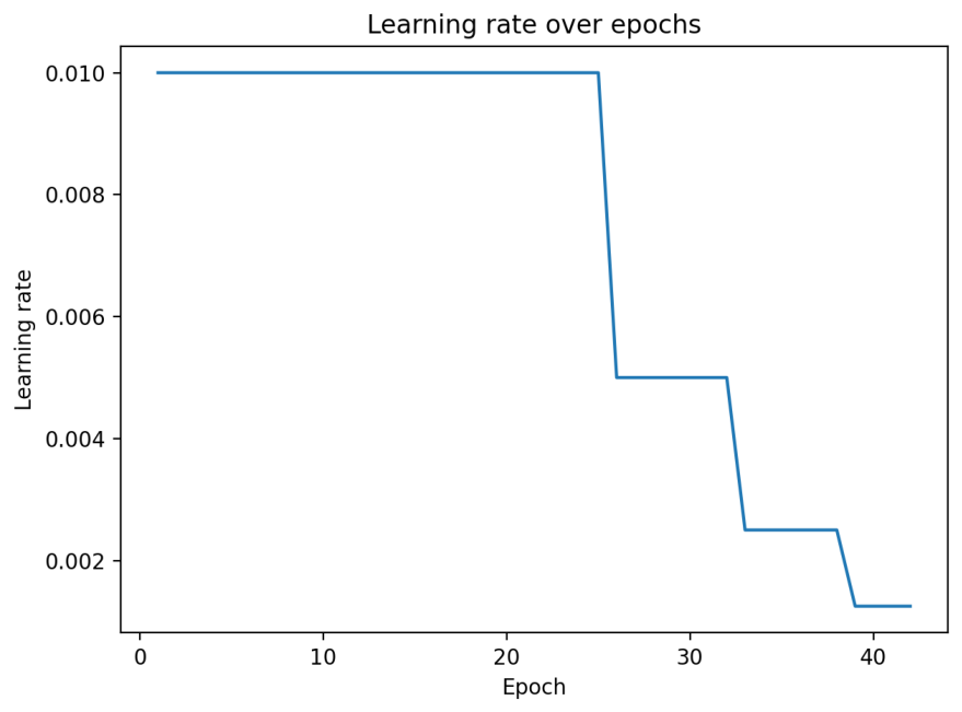
Figure 2.
Distribution of Environmental Performance (EP) with threshold .
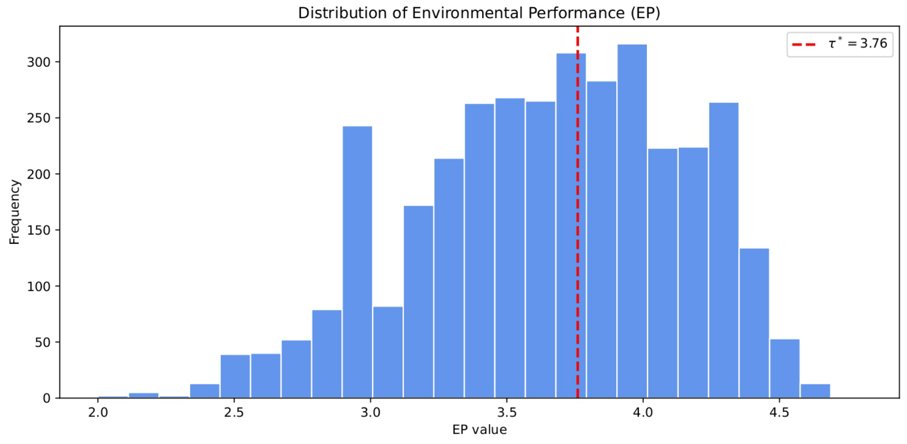
Figure 3.
Firm splits for training, validation, and testing.
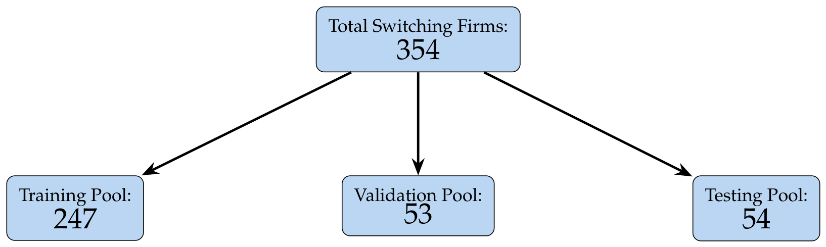
Figure 4.
Distribution of percentage differences in turnover.
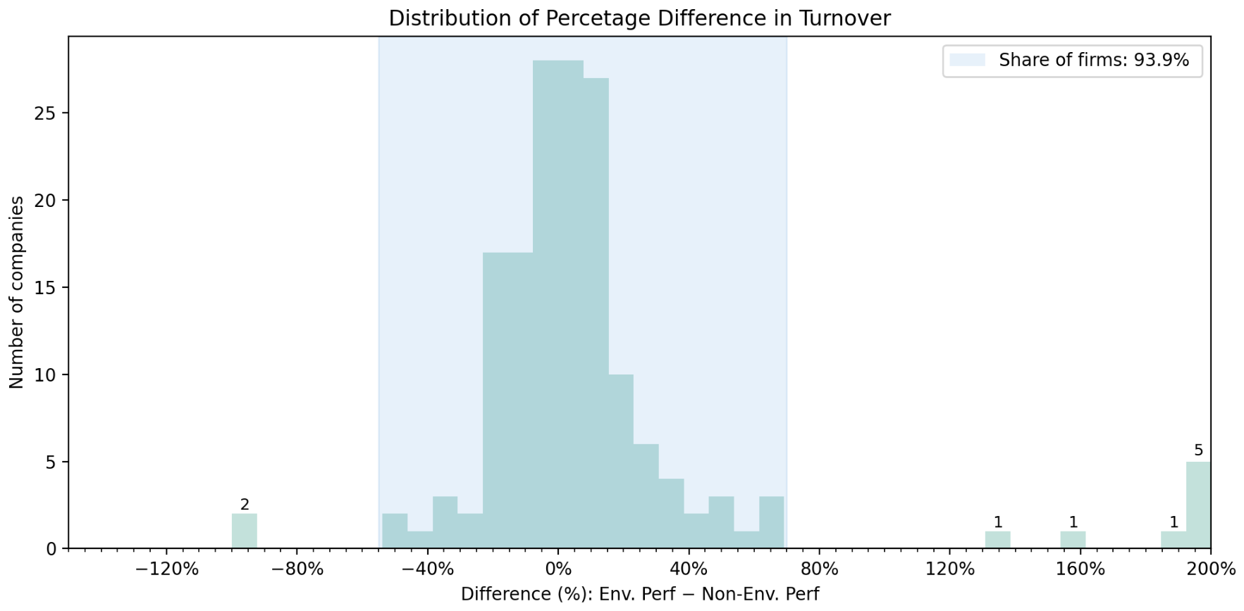
Table 1.
Industry Distribution of Companies.
| Industry | Percentage (%) |
|---|---|
| Production (Manufacturing and Industrial) | 36.47 |
| Construction | 37.48 |
| Trade | 12.74 |
| Transportation | 6.22 |
| Energy/Utilities | 5.78 |
| Agriculture | 1.04 |
| Other | 0.27 |
Table 2.
LSTM-Dense Grid Search Results.
| LSTM | DENSE | Train MSE | Validation MSE | Train MAE | Validation MAE |
|---|---|---|---|---|---|
| 4 | 2 | 0.006567 | 0.005287 | 0.065616 | 0.057821 |
| 4 | 4 | 0.005883 | 0.005447 | 0.061302 | 0.060587 |
| 4 | 8 | 0.006341 | 0.004470 | 0.064325 | 0.054290 |
| 4 | 16 | 0.005262 | 0.005676 | 0.057919 | 0.061133 |
| 4 | 32 | 0.006750 | 0.005228 | 0.064220 | 0.058531 |
| 8 | 2 | 0.005604 | 0.004686 | 0.059861 | 0.056398 |
| 8 | 4 | 0.005751 | 0.005790 | 0.060041 | 0.060592 |
| 8 | 8 | 0.005586 | 0.004983 | 0.059238 | 0.055876 |
| 8 | 16 | 0.005285 | 0.005438 | 0.058306 | 0.059893 |
| 8 | 32 | 0.005575 | 0.005733 | 0.059432 | 0.061362 |
| 16 | 2 | 0.006169 | 0.004933 | 0.062883 | 0.055495 |
| 16 | 4 | 0.005239 | 0.004748 | 0.057673 | 0.054962 |
| 16 | 8 | 0.005720 | 0.005760 | 0.061037 | 0.058106 |
| 16 | 16 | 0.005708 | 0.005268 | 0.059927 | 0.058052 |
| 16 | 32 | 0.005065 | 0.005226 | 0.055428 | 0.056580 |
| 32 | 2 | 0.006265 | 0.005312 | 0.064173 | 0.057456 |
| 32 | 4 | 0.006720 | 0.005336 | 0.064726 | 0.056268 |
| 32 | 8 | 0.005376 | 0.005573 | 0.058381 | 0.058158 |
| 32 | 16 | 0.006180 | 0.004669 | 0.062948 | 0.053917 |
| 32 | 32 | 0.005906 | 0.005250 | 0.060647 | 0.057874 |
| 64 | 2 | 0.005634 | 0.005141 | 0.059321 | 0.056218 |
| 64 | 4 | 0.006024 | 0.005072 | 0.061874 | 0.056851 |
| 64 | 8 | 0.005798 | 0.004928 | 0.060374 | 0.055546 |
| 64 | 16 | 0.006046 | 0.004891 | 0.062450 | 0.057660 |
| 64 | 32 | 0.005796 | 0.004758 | 0.061017 | 0.055220 |
The table reports training and validation performance for each LSTM–Dense layer configuration. The 32-16 row (shaded) represents the best-performing model based on validation MAE. MSE denotes the mean squared error, while MAE denotes mean absolute error.
Table 3.
Validation performance across learning rates.
| Learning rate | Train MSE | Val MSE | Train MAE | Val MAE |
|---|---|---|---|---|
| 0.001 | 0.006081 | 0.006430 | 0.063017 | 0.063200 |
| 0.005 | 0.004894 | 0.005103 | 0.054519 | 0.057413 |
| 0.010 | 0.006068 | 0.004947 | 0.061644 | 0.057168 |
| 0.050 | 0.005528 | 0.005484 | 0.058360 | 0.060702 |
| 0.100 | 0.004021 | 0.006273 | 0.049121 | 0.065070 |
Table 4.
Batch Size Sensitivity Analysis.
| Batch | Train MSE | Validation MSE | Train MAE | Validation MAE |
|---|---|---|---|---|
| 8 | 0.004981 | 0.005726 | 0.055968 | 0.062380 |
| 16 | 0.009182 | 0.004781 | 0.072864 | 0.054470 |
| 32 | 0.005636 | 0.004665 | 0.059451 | 0.054349 |
| 64 | 0.004842 | 0.004937 | 0.055849 | 0.055777 |
| 128 | 0.004963 | 0.005615 | 0.056386 | 0.059595 |
The table reports training and validation performance across different batch sizes, holding the LSTM (32 units) and Dense (16 units) architecture fixed. The highlighted row corresponds to the best-performing configuration based on validation MAE. MSE denotes mean squared error, while MAE denotes mean absolute error.
Table 5.
Final hyperparameter configuration for the dual-input LSTM model.
| Parameter | Value | Description |
|---|---|---|
| Sequence length (L) | 2 | Number of past years used as historical input window. |
| LSTM units | 32 | Number of memory cells in the LSTM layer. |
| Dense units | 16 | Size of the fully connected layer for the current-year input. |
| Learning rate | 0.01 | Step size for gradient updates. |
| Batch size | 32 | Number of samples per weight update. |
| Epochs | 200 | Upper bound on training iterations. |
Table 6.
Performance summary of the dual-input LSTM for EP prediction.
| Dataset | MSE | MAE |
|---|---|---|
| Training set | 0.0051 | 0.0565 |
| Validation set | 0.0054 | 0.0598 |
| Test set | 0.0096 | 0.0731 |
Table 7.
Description of notations used in the MILP.
| Symbol | Description |
|---|---|
| Lowest EP value recorded for firm i during 2019–2024. | |
| Highest EP value recorded for firm i during 2019–2024. | |
| Smallest minimum EP observed among all firms, lower bound of the feasible threshold range. | |
| Largest maximum EP observed among all firms, upper bound of the feasible threshold range. | |
| Small positive constant used to enforce a strict relationship relative to the starting EP level. In the implementation . | |
| Distance between the adjusted lower bound and the global minimum, i.e.: . | |
| Distance between the global maximum and the firm’s maximum EP, i.e.: . |
Table 8.
Summary of MILP outcome.
| Type | Value |
| Total firms | 593 |
| Switching firms | 370 |
| Firms always performant | 59 |
| Firms always underperforming | 164 |
Table 10.
Learning Rate Grid Search
| LR | Train MSE | Validation MSE | Train MAE | Validation MAE |
|---|---|---|---|---|
| 0.0001 | 15.187823 | 17.679247 | 3.652274 | 3.943899 |
| 0.0010 | 0.028572 | 0.027228 | 0.126194 | 0.131358 |
| 0.0050 | 0.031251 | 0.031384 | 0.135617 | 0.134878 |
| 0.0100 | 0.038281 | 0.025971 | 0.145924 | 0.124658 |
| 0.0200 | 0.025871 | 0.036938 | 0.118399 | 0.152327 |
| 0.0300 | 0.038598 | 0.031294 | 0.155562 | 0.141465 |
The table reports training and validation metrics for various learning rates, ordered from the lowest to the highest learning rate, using the {LSTM, Dense} configuration {8, 4}. The shaded row represents the best-performing configuration based on validation MAE.
Table 11.
Batch Size Grid Search.
| Batch Size | Train MSE | Validation MSE | Train MAE | Validation MAE |
|---|---|---|---|---|
| 8 | 0.030005 | 0.023762 | 0.135235 | 0.123635 |
| 16 | 0.034707 | 0.035279 | 0.136103 | 0.131759 |
| 32 | 0.033486 | 0.028942 | 0.136662 | 0.130142 |
| 64 | 0.055340 | 0.060975 | 0.164901 | 0.160916 |
| 128 | 0.406137 | 0.539402 | 0.396880 | 0.456664 |
The table reports training and validation metrics for different batch sizes, ordered from the smallest to the largest batch size, using the {LSTM, Dense} configuration {8, 4}, with learning rate . The shaded row represents the best-performing configuration based on validation MAE.
Table 12.
L2 Regularization Grid Search.
| Train MSE | Validation MSE | Train MAE | Validation MAE | |
|---|---|---|---|---|
| 0 | 0.029638 | 0.022852 | 0.130175 | 0.120169 |
| 0.00001 | 0.031143 | 0.028497 | 0.128479 | 0.123605 |
| 0.0001 | 0.047815 | 0.037915 | 0.136256 | 0.123748 |
| 0.001 | 0.133138 | 0.122263 | 0.150826 | 0.129564 |
| 0.01 | 0.787448 | 0.805581 | 0.185165 | 0.201266 |
The table reports training and validation metrics for varying L2 regularization strengths (), ordered from the lowest to the highest , using the {LSTM, Dense} configuration {8, 4}, learning rate , and batch size 8. The shaded row represents the best-performing configuration based on validation MAE.
Table 13.
Hyperparameters of the dual-input LSTM for Turnover prediction.
| Parameter | Value | Description |
|---|---|---|
| Sequence length (L) | 5 | Number of past years used as the historical input window. |
| LSTM units | 8 | Number of memory cells in the LSTM layer. |
| Dense units | 4 | Size of the fully connected layer for the current-year input (ReLU). |
| Learning rate | 0.01 | Step size for gradient updates (initial). |
| Batch size | 8 | Number of samples per weight update. |
| Epochs | 500 | Upper bound on training iterations. |
| Regularization | L2, | Applied to LSTM (kernel, recurrent, bias) and Dense layers (kernel). |
Table 14.
Final Model Performance Summary.
| Metric | Train | Validation |
| MSE | 0.0218 | 0.0471 |
| MAE | 0.1089 | 0.1633 |
| MAPE (%) | 11.87 | 14.79 |
| Last Learning Rate | 0.0034 | |
| Epochs Trained | 278 | |
MAPE denotes the Mean Absolute Percentage Error and measures the average absolute percentage difference between the model’s predictions and the historical Turnover.
Table 15.
Prediction Error Summary for the Test Set.
| Statistic | Hist. Turnover | Pred. Turnover | Abs. Error | Abs. Perc. Error (%) |
| Count | 54 | |||
| Mean | 1.7415×10⁹ | 1.7685×10⁹ | 1.6430×10⁸ | 15.18 |
| Std | 4.0255×10⁹ | 3.9589×10⁹ | 3.7263×10⁸ | 17.40 |
| Min | 0.00 | 2.47×10⁷ | 3.27×10⁵ | 0.23 |
| 25% | 1.46×10⁸ | 1.38×10⁸ | 1.42×10⁷ | 4.28 |
| Median | 4.50×10⁸ | 4.44×10⁸ | 4.58×10⁷ | 10.22 |
| 75% | 1.09×10⁹ | 1.05×10⁹ | 1.20×10⁸ | 18.82 |
| Max | 2.40×10¹⁰ | 2.20×10¹⁰ | 2.01×10⁹ | 86.98 |
Table 16.
Summary of Estimated Turnover Effects (values in percentage points).
| N | Effect by Direction | |||
| 143 | Negative | Positive | ||
| Overall mean effect | — | |||
| Overall median effect | — | |||
| Count (nr) | — | 62 | 81 | |
| Mean (within group) | — | 13.69 | 16.83 | |
| Std. dev. | — | 11.61 | 12.30 | |
| Max | — | 51.34 | 58.21 | |
| Min | — | 0.65 | 0.10 | |
| Median | — | 9.38 | 15.61 | |
| 75th percentile | — | 18.37 | 23.48 | |
Disclaimer/Publisher’s Note: The statements, opinions and data contained in all publications are solely those of the individual author(s) and contributor(s) and not of MDPI and/or the editor(s). MDPI and/or the editor(s) disclaim responsibility for any injury to people or property resulting from any ideas, methods, instructions or products referred to in the content. |
© 2026 by the authors. Licensee MDPI, Basel, Switzerland. This article is an open access article distributed under the terms and conditions of the Creative Commons Attribution (CC BY) license (http://creativecommons.org/licenses/by/4.0/).
Copyright: This open access article is published under a Creative Commons CC BY 4.0 license, which permit the free download, distribution, and reuse, provided that the author and preprint are cited in any reuse.