

Submitted:
02 September 2026
Posted:
03 September 2026
You are already at the latest version
Abstract
Similarity reductions of unsteady two-dimensional flow are almost always constructed from the boundary-layer equations, in which streamwise diffusion and the transverse momentum balance are discarded at the outset. We ask when such a reduction is also a reduction of the full Navier–Stokes equations, using the diffusion-time-scale variables \(\eta=y/\delta(x)\), \(\tau=\nu t/[\delta(x)]^2\) of Sun [32]. All chain rules collapse onto the stretching operator \(\mathcal{D}=\eta\partial_\eta+2\tau\partial_\tau\), both momentum equations transform in closed form, and the discarded terms enter through a single coefficient \(\varepsilon=\delta'^2\). For the family \(U=Cx^m\) the reduction closes in \( (\eta,\tau) \) alone if and only if \(m=1\) or \(m=-1\). The second case is a diverging channel, and there the reduced problem is elliptic in \( (\eta,\tau) \), with principal symbol \( (\xi_\eta^2+\varepsilon s^2)^2 \) degenerating only on \(\tau=0\): the similarity time is not an evolution variable, data must be posed at both ends, and marching in \(\tau\) is inconsistent. Solving the resulting boundary-value problem, we find that the influence of the terminal condition decays as \(\exp[-(T-\tau)/L]\), and that \(L\) collapses on the wedge half-angle, \(L\simeq2.2\,\theta_w\), to within 14% over a factor of 16 in Reynolds number, the prefactor depending on the sense of the flow but the scaling not. The upstream influence is therefore geometric rather than viscous: it vanishes with the divergence angle and is essentially independent of Re, so that marching is safe in slender geometries at any Reynolds number and unsafe in wide ones however viscous. Three exact solutions in elementary functions, obtained from the invariance of \(\zeta=\eta/\sqrt{\tau}=y/\sqrt{\nu t}\) under \( D \), and the Jeffery–Hamel steady limit, serve to verify the reduction throughout.
Keywords:
2D laminar flow
; exact solutions
; similarity transformation
1. Introduction
Exact solutions of the Navier–Stokes equations are rare [33,34,35], and those that exist are almost all steady or one-dimensional. The classical similarity solutions of Blasius [5] and Falkner Skan [9], with the numerical integration of Hartree [15], are steady; the unsteady counterparts are far fewer, and are reviewed by Riley [26]. For the two-dimensional unsteady problem the principal difficulty is that a similarity variable built on one intrinsic time scale generally reintroduces the coordinate that was to be eliminated through the other. Sun [32] proposed a way around this by promoting time itself to a similarity variable, measured on the transverse diffusion time scale identified by Stuart [31]:
Applying (1) to the truncated system
Sun obtained the single equation
his Equation (19), with
and showed that , , are simultaneously free of x for the power-law family . Equation (3) is a genuine reduction of (2), and we confirm it below.
As a matter of attribution it should be recorded at the outset that this reduction of the truncated system is not new. Ma and Ma Hui [20] obtained, by Lie group methods, all group-invariant similarity solutions of precisely the system (2), classified them into six classes, and observed that the classification contains all previously known solutions as special cases. The transformation (1) is a member of their Class VI, as we show explicitly in Section 4.1: the generator it quotients by lies in their symmetry algebra, and their invariants are related to by an invertible change of variables with . What is new in [32] is not the reduction but its parametrisation—the use of a scaling length and of the diffusion time , which brings the three parameters (4) and the operator structure of Section 3 into view. That is a genuine gain in transparency, and it is what makes the present analysis possible; it is not a new similarity solution.
The present work asks a different and, we believe, prior question. The system (2) is not the Navier–Stokes system: the transverse momentum equation has been replaced by , and the streamwise diffusion has been dropped. Does the transformation (1) reduce the full equations? If it does, for which members of the family, and is the resulting system well-behaved—does it admit a sensibly posed problem with solutions that are bounded and that satisfy all of the conditions imposed on them?
We answer these questions completely, and the answer has a consequence we did not anticipate. The transformation does act cleanly on the full system: both momentum equations transform in closed form, and the transverse equation, far from being trivial, is a compact quadrature for the pressure. The discarded terms enter through a single coefficient , which is free of x in exactly two cases, and . The first is the stagnation-point family, for which and the discarded terms vanish identically. The second is a diverging channel, for which they do not: they survive with a finite coefficient, and they make the reduced problem elliptic in . The similarity time is then not an evolution variable, data must be posed at both ends of the interval, and the natural expectation that one may prescribe the state at and integrate forward—correct for the truncated equation (3), which is first order in —does not survive the restoration of the discarded terms.
Solving that boundary-value problem, we find that the influence of the terminal condition decays exponentially backwards in , over a length L that collapses on the wedge half-angle rather than on the Reynolds number,
to within over a factor of 16 in . The upstream influence introduced by streamwise diffusion is therefore geometric, not viscous: it vanishes with the divergence angle of the channel and is essentially independent of . Marching in the similarity time is consequently justified in slender geometries at any Reynolds number, and unjustified in wide ones however viscous. This is the central result of the paper.
Along the way the transformation supplies three exact solutions in elementary functions, and reproduces Jeffery–Hamel flow as a steady limit. These are classical flows. We present them not as new solutions but as verification: each is recovered here from the full equations with no term discarded, so each exercises the transformed operators end to end.
The distinction matters for what follows. Ma Hui [20] classifies reductions of the truncated system (2); the questions asked here concern the full system (Section 2), on which that classification is silent.
Throughout we adopt Sun’s notation, including (4), so that every statement can be compared line by line with [32]. Following the aim of this study, no use is made of, and no appeal is made to, approximations of thin-layer type: the object of interest is the transformed system itself.
The paper is organised as follows. Section 2 states the full problem and Section 3 develops the operator algebra of the transformation, the velocity field, and the identity satisfied by continuity. Section 4 collects the similarity constraints and the derived quantities m, n, , . Section 5 and Section 6 transform the two momentum equations exactly. Section 7 establishes the closure condition and derives the reduced system and its type. Section 8 treats the admissible data. Section 12 solves the channel problem numerically and establishes the scaling (5), the Reynolds-number sweep being given in Section 12.4; Section 13 concludes. Appendix A collects operator identities, Appendix B the coefficient dictionary, Appendix C the cancellation bookkeeping, and Appendix D the verification protocol.
2. Formulation
We consider the unsteady plane motion of an incompressible Newtonian fluid of constant density and kinematic viscosity , governed by the full Navier–Stokes system
with and so on. Continuity is satisfied identically by
and elimination of p between (6b) and (6c) gives the vorticity form
Equations (6b) and (6c) are equivalent to (8) together with two quadratures for and ; the compatibility of those quadratures, , is precisely (8). This equivalence will be used in Section 7 as an independent check.
Primes on functions of x alone denote , so and ; subscripts denote partial derivatives of f. The length in (1) is a scaling function to be fixed by the similarity constraints, and is a reference velocity; neither is given an interpretation beyond that.
3. The Transformation
3.1. Chain Rules and the Stretching Operator
Under (1),
which are Sun’s relations and . The two streamwise derivatives differ only by the factor 2, because while . Introducing the stretching operator
the chain rules for any collapse to
is the generator of the scaling group under which (1) is invariant, assigning weight 1 to and 2 to . More generally, for a product with and
repeated use of (11) gives the two identities on which the whole calculation rests,
Identities involving are collected in Appendix A.
3.2. Velocity Components
Using and, from (4), , the transverse component takes the compact form
The grouping (17) is the single most useful consequence of the operator notation: v is times a fixed linear combination of and f, with the two similarity parameters as coefficients.
3.3. Continuity
From (16),
where has been used, so that for every f. This is a nontrivial check because does not commute with ; the commutator supplies exactly the term needed for the cancellation.
4. Similarity Constraints and Derived Quantities
The three parameters (4) are not independent. From and one has , while follows directly from (4). Hence
which are Sun’s relations. Integrating the second and eliminating with gives, for ,
Positivity of requires ; no modulus is then needed in (20).
It is worth being explicit that the power law is forced rather than chosen. The reduction requires , and to be free of x, and (19) then integrates uniquely to (20) for , the exceptional case giving the exponential family , which is the limit . No other external flow admits constant coefficients. The restriction to in what follows is therefore not a loss of generality within the class of similarity reductions of this transformation, and the closure condition of Section 7.2 is a statement about the whole class.
Three derived quantities recur. With , equation (12) gives
so that and, usefully, and identically. Writing
for the local Reynolds number, equation (20) gives and hence
The parameter will turn out to control every term that distinguishes the full system from the truncated one. Since ,
the last equivalence following from . Equivalently, means . Table 1 lists the two cases of [32] in this language.
4.1. Relation to the Lie-Group Classification
Before proceeding it is worth locating the transformation (1) within the group-theoretic classification of the unsteady two-dimensional problem given by Ma and Ma Hui [20], who used Lie group methods to derive all group-invariant similarity solutions of the system they denote (2), which is the truncated system (2) above.
A similarity reduction is determined by the subgroup with respect to which one quotients, not by the symbols used to name the invariants. With and from (21), the variables (1) are
and the vector field annihilating both is

Table 2.
Summary of the parameters. The first three are those of Sun [32]; the rest are derived. All are constants once the similarity conditions of Section 4 hold, with the single exception of , whose x-dependence is the obstruction analysed in Section 7.2.
Table 2.
Summary of the parameters. The first three are those of Sun [32]; the rest are derived. All are constants once the similarity conditions of Section 4 hold, with the single exception of , whose x-dependence is the obstruction analysed in Section 7.2.
| symbol | definition | meaning | closure |
|---|---|---|---|
| growth of | |||
| pressure gradient | |||
| growth of the scale | |||
| m | exponent in | — | |
| n | growth rate of | ||
| operator shift | singular at | ||
| local Reynolds number | const. | ||
| streamwise diffusion | const. | ||
| wedge half-angle | sets L |
The symmetry algebra of Ma Hui [20], obtained by the standard infinitesimal method [6,22,23], is spanned by , and , together with two infinite-dimensional subalgebras that are excluded by the boundary conditions. Matching the coefficients of , and in against (26) gives and , consistently, so that
and the reduction (1) is a group-invariant reduction under a subgroup already classified in [20].
More specifically, it is their Class VI, whose invariants are , with . Setting
one has the exact identities
an invertible change of variables between and , while is reproduced by with the same value (28) of q. Both (27) and (29) hold for every . For , for instance, , , , , and , .
Two remarks follow. First, the reduction of the truncated system is not new, and [20] states that its classification contains all previously known solutions as special cases; the parametrisation by is what is new, and it is a real gain in transparency, since the parameters (4) and the operator (10) are not readable from . We note also that the dimensional argument of [32] cannot escape the classification, the group-theoretic method containing dimensional analysis [3,7] as a special case [20,23].
Second, and more to the present purpose, the classification of [20] is a classification of the truncated system. Their Class VI is reduced to ordinary differential equations in two cases only, and the two-variable system in is left as such. Nothing in that work bears on the full Navier–Stokes system, which is the subject of Section 5, Section 6, Section 7, Section 8 and Section 9.4 below; the closure condition , the transverse balance (41) and the type of the reduced operator are statements about equations they did not treat.
5. The Streamwise Momentum Equation
The streamwise diffusion follows from (14) with , i.e. :
which, using , and (23), collapses to the remarkably simple group
Finally, we do not prescribe the pressure gradient. Every other term of (6b), divided by , is a function of , so we simply define the scaled streamwise pressure gradient
Substituting into (6b) and dividing by then gives the exact transformed streamwise momentum equation
Equation (35) contains equation (3) as the special case obtained by discarding S and imposing the closure , which is what the substitution of the truncated system (2) amounts to:
Equation (35) has been checked term by term against (6b) in physical variables (Appendix D).
6. The Transverse Momentum Equation
The transverse equation is dispatched at the outset in the truncated formulation by the statement . Under the transformation it is in fact a well-defined and compact object, and we now derive it.
Anticipating the structure, note first what kind of equation it must be. Once f is known, every term of (6c) is determined except . The transverse equation therefore introduces no new unknown function of two variables: it is a first-order quadrature in that delivers the transverse pressure.
6.1. Derivatives of v and the Scaled Pressure
The operator rather than in is the kinematic signature of the transverse velocity: the extra unit comes from differentiating the prefactor . Defining the scaled pressure
and noting that so that every term of (6c) carries the common factor , division by that factor gives the exact transformed transverse momentum equation
where is rewritten with and (23). Equations (35) and (40) are structurally identical—diffusion, unsteadiness, convection, streamwise diffusion—with the unknown displaced from f to .
6.2. Closed Form
Equation (40) may be expanded entirely in f. The key step is to eliminate the third derivative appearing in by means of (35). When this is done a large number of terms cancel identically—in particular every term of the form times a quadratic product of derivatives of f (Appendix C)—and the result condenses to
This answers the question of what form the transverse momentum equation takes: a first-order ordinary differential equation in for the pressure, whose right-hand side is a known bilinear functional of f and its -derivatives. Three features deserve comment.
(i) Weighting pattern. The unsteady contributions enter with the weights 1, and , that is, as successive powers of . The same pattern appears in (35), where the single unsteady group carries the weight ; the transverse equation is quadratic in it because v already contains one power of through (17).
(ii) Second-order unsteadiness. Equation (41) contains , whereas (35) contains only first -derivatives of . This is not an inconsistency: is obtained by differentiating (35) with respect to and is therefore known, not an additional unknown.
(iii) Truncated closure. Setting and reduces (41) to the compact form
which is the transverse pressure generated by any solution of (3). Equation (42) does not vanish. This is not an inconsistency in the truncated system, which imposes as part of its approximation, but it does quantify what that approximation costs: the motion described by (3) generates a transverse pressure gradient of the size (42), which the truncation discards. Equation (41) recovers it at no extra cost once f is known.
6.3. Verification at the Wall
At a fixed impermeable wall one has for all x and t, whence there, and (6c) collapses to the exact identity
Impermeability requires for all , hence also and, from (17) and , ; likewise and vanish at . Both (40) and (41) then reduce, using from Section 8, to
in exact agreement with (43). The wall pressure gradient is thus fixed by the wall shear and its rate of change,
and it vanishes only in the trivial case of a -independent wall shear with .
7. Closure of the Full System
7.1. Pressure Compatibility
7.2. The Closure Condition
Everything so far is exact. The reduction to two independent variables, however, requires that P, and every coefficient in (35), (40) and (46) be free of x. The parameters are constants by construction, and the only remaining coefficient is . By (23),
which is free of x in exactly two circumstances: either the numerator vanishes, , or the denominator is constant, . Hence
Proposition 1.
The two cases are of quite different character.
(i) , , . Here , so is constant and : the streamwise-diffusion operators are not small, they are absent. Since one has , the operator drops out of the streamwise derivative altogether, and . The velocity field is with and , independent of x, so that identically. This is the stagnation-point family, treated in Section 9.2.
(ii) , , . Here is a genuine constant, , and ; the streamwise-diffusion operators are present and finite. This is the channel family, treated in Section 7.3 and Section 9.4.
For every other m the transformed equations are exact but retain an explicit x-dependence through ; they reduce only after is set to zero, which returns the truncated system (2) and equation (3). We have confirmed all of this numerically: evaluating P and from the physical equations against (35) and (40) agrees for every m tested, while the reduction to alone holds only for (Appendix D).
A third possibility should be mentioned, because it is the one exploited in Section 9.1: for particular solutions, rather than for the equation family, the groups may vanish even when . This occurs whenever and , and it yields exact solutions of the full system at values of m for which the general reduction fails.
7.3. The Reduced System for
Set . Then , , , and with constant. The normalisation gives , and . The velocity field is
and the two momentum equations become
with P fixed by (46). Discarding the groups and setting in (49) returns
which follows here directly from equation (3) with .
Eliminating P and through (46) gives the single governing equation. Writing with, from (14),
equation (8) transforms, for , into
We have checked that (53) is identical to (49) combined with (46) and (50), and, independently, that it reproduces equation (8) evaluated in physical variables (Appendix D).
7.4. Type of the Reduced Operator
Equation (53) is fourth order in , but it is also, and less obviously, fourth order in : the operator carries , and already contains . Its type is best read off from the symbol. Let and
be the symbol of . From (14) the symbol of acting on functions of is , so the principal symbol of (53) is
The quadratic form is positive definite for every when : it vanishes only if and . Three consequences follow.
First, the reduced equation (53) is a fourth-order elliptic equation in . This is as it must be: the full Navier–Stokes system is elliptic in the spatial variables, and the similarity variable mixes t with x, so it inherits the ellipticity of the streamwise direction. Data must therefore be posed on the whole boundary of the domain, and cannot be marched.
Second, the degeneracy is confined to , where the form collapses to . The line is therefore a characteristic boundary, and the number of conditions that may be imposed on it is not the number appropriate to an elliptic boundary but is fixed instead by the Fichera condition, which is worked out in Section 8.3.
Third, and in sharp contrast, the truncated equation (3) is recovered at , where the symbol degenerates to throughout: the truncated equation is parabolic and first order in , and is an evolution variable for it. The distinction is not a technicality. Any procedure that prescribes f at and advances in is solving the truncated problem, not the Navier–Stokes problem, however small may be; and since multiplies the highest -derivatives, is a singular limit.
This is the principal structural consequence of retaining the discarded terms. It is a statement about how the problem must be posed, not about whether it can be solved: Section 12.3 shows that the resulting upstream influence is exponentially localised, so the practical penalty is mild and quantifiable. The transformation (1) is exact and elegant, and it does reduce the full system when ; but the reduced problem is not an evolution problem, and solutions constructed by marching in —or obtained in closed form from the parabolic truncation—carry no guarantee of solving the elliptic problem to which the Navier–Stokes equations actually reduce.
8. Admissible Data
8.1. Wall Conditions
Let the wall be impermeable and at rest. No slip requires
while impermeability requires , that is, from (17),
with A constant. Condition (57) is weaker than , which is what one might write down by analogy with the steady theory. It is nevertheless correct: is independent of x whenever is, which is exactly (57), so the wall remains a streamline and vanishes on it.
For equation (57) gives , and this accounts structurally for the term in Sun’s closed-form solution, his Equation (26); it also reproduces his wall condition, Equation (36), . For it gives , and A may be absorbed into the definition of . Note that is bounded as only if or ; for the only admissible wall behaviour is . It was in the derivation of (44) that this condition was used, and one may check that the combination appearing there vanishes identically for .
8.2. The Outer Boundary
The condition , inherited from the truncated problem, requires care for the full system, and for it must be abandoned altogether. Writing as and substituting in (52) gives
which grows linearly in and does not decay. The reason is not a defect of the transformation: for the state , has and is rotational, so there is no irrotational outer region to match to and no admissible decay condition on .
The resolution is supplied by the exact solution of Section 9.4: for the natural domain is not a half plane but a channel bounded by a second wall, the walls being surfaces of constant . The conditions at are then of the same kind as those at ,
with fixed by the volume flux, and the difficulty in (58) does not arise. We adopt this domain from here on. Since the reduced operator is elliptic, conditions are required on every remaining portion of the boundary of the rectangle , including ; the truncated problem, being parabolic, needs none there.
At the line is characteristic and the count must be obtained from the Fichera condition; this is done next.
8.3. The Characteristic Form
For write the reduced problem as the coupled pair, with signs chosen so that the characteristic form is nonnegative,
In the coordinates both operators share the second-order coefficient matrix
whose quadratic form is with and , in agreement with (55). Thus everywhere, with for and only on .
8.4. The Fichera Function
For a second-order operator with nonnegative characteristic form, the boundary of the domain splits into the non-characteristic part and the characteristic part, on which the Fichera function
splits it further [17] into , and . Data may be assigned on and must not be assigned on [10,21]. The classical check is the heat operator , for which at and at , giving one condition initially and none finally.
8.5. Classification of the Boundary
On the inner normal is , and (63) gives
as . Hence belongs to for (60) and to for (61), and the admissible data there are
Proposition 2.
exactly one condition, prescribing , and no condition on f.
Two remarks. First, the limit comes entirely from the term : the contributions cancel down to and the convective contribution vanishes with . It is therefore the unsteady term alone that makes an admissible data surface at all; for a steady problem there and no data could be assigned. Second, the result explains why an attempt to prescribe a velocity profile at is ill-advised: is not free data but is determined by (60) from and the conditions on the remaining boundaries.
The other portions of are non-characteristic. On one has ; on , ; and similarly as . All three lie in and require data. Since the coupled system is of fourth order, two conditions are needed on each. At the wall both are carried by f, namely and from (57); there is no independent condition on there, and must be recovered from (60) as part of the solution, exactly as in any streamfunction–vorticity formulation.
The requirement of data on deserves emphasis, since it is the practical content of the ellipticity established in Section 7.4: the reduced problem is a two-point boundary-value problem in , not an initial-value problem, and cannot be marched. Table 3 summarises the count.
8.6. The Truncated System and the Locus
Setting gives , so and every line is characteristic. At one still finds and one condition, as expected of a parabolic problem. At , however, the inner normal is and
written for general using the coefficient of the convective group with . The sign is not fixed: no data are required where , but data are required where .
The reason is kinematic. Along a fluid particle path,
which follows from , and , and which we have verified for general . The similarity time therefore increases along a path only where , is stationary on the locus
and decreases beyond it. The truncated equation, although parabolic, thus possesses no globally defined time-like direction: it must be integrated in the direction of increasing on one side of (69) and of decreasing on the other, and (69) is itself a characteristic across which information passes in neither direction. This is a structural obstruction to obtaining well-behaved solutions of the truncated system by marching, and it is independent of the discretisation.
Where the locus is , which for is
The coefficients of the equation are perfectly regular there; what degenerates is the orientation of the characteristic direction, not the operator. This is consistent with the conclusion of [32] that is not a singular point, and it identifies what does occur at that value.
Finally, and in the positive direction: for the operator is elliptic, has no characteristic direction, and the locus (69) carries no special status whatever. The terms discarded in passing to the truncated system act as a regularisation of the degeneracy. The price, as Section 7.4 shows, is that the problem ceases to be an evolution problem; the two difficulties are two faces of the same fact, and it is the second that must be confronted if well-behaved solutions are to be constructed.
9. Exact Solutions
The transformed system admits several families of exact solutions. We begin with the unsteady ones, which are the object of this study, and close with the steady limit of the channel family.
9.1. The -Invariant Reduction
The transformation carries with it a distinguished second-order variable. Since assigns weight 1 to and weight 2 to , the ratio
so that is an invariant of the stretching group and any function of alone is annihilated by . Moreover has a direct meaning: from (1),
independently of and hence of x. This suggests the ansatz
under which f is an eigenfunction of with eigenvalue . The consequences are immediate and strong. From (17),
so the transverse velocity is proportional to f itself; and , so that .
Substituting (73) into the transformed streamwise equation (3) and multiplying by leaves three groups, of orders , and :
A reduction to a single ordinary differential equation in requires the three exponents 0, and to collapse to at most one. They cannot all coincide, so exactly one pair must be made equal, and the third group must then vanish identically. Enumerating the three pairings:
- , i.e. ; the third exponent is 2 and the group must vanish, so .
- , i.e. ; both groups are of order and combine to , which vanishes either for or, if , only for the trivial .
- , i.e. ; the group must vanish identically, which requires both coefficients in the second bracket of (75) to be zero, giving and hence .
Hence
Proposition 3.
The ansatz (73) reduces the transformed equation to an ordinary differential equation in exactly three cases: with (that is ), and with , (that is ).
A single criterion governs which of these also solve the full equations. From (74) the transverse velocity vanishes when , and the streamwise-diffusion group (33) evaluates on the ansatz to , which vanishes at because . Therefore
and the solution is exact for the full Navier–Stokes system, whatever the value of m. The branches () and () both satisfy (76); the branch does not, and solves only the truncated system. We take the three in turn.
9.1.1. The Branch : An Exact Unsteady Solution
For the second and third groups of (75) coincide in order and combine to , which vanishes with , and the reduction is simply
whose general solution is elementary,
Every member of this two-parameter family is an exact solution of the transformed unsteady equation, at every finite , with no approximation and no restriction to small or large time. In particular the choice , , that is
satisfies the complete set of conditions
simultaneously and for all , as does the complementary choice , , for which and the wall and outer conditions are interchanged. We have verified the vanishing of the residual symbolically (Appendix D).
Two features deserve comment.
First, (79) solves not only the truncated equation but the full Navier–Stokes system, even though is not one of the two cases of Section 7.2. The reason is the mechanism noted there. From (74) with , , ,
so identically, and the whole transverse equation (40) collapses to . Likewise , so that the streamwise-diffusion group (33) reduces to , which vanishes because at . The groups are therefore not neglected but annihilated: the solution is exact for the full equations. In physical variables it is
the Rayleigh–Stokes shear flow [25,30], listed by Ma Hui [20] as one of the few unsteady similarity solutions that also satisfy the Navier–Stokes equations, and the starting point of the impulsive-start analyses of Stewartson [29], Hall [13] and Dennis [8]. The flow is classical; what is recorded here is that it is an exact solution of the transformed unsteady equation (3) meeting all of the conditions imposed on that equation, and that it is reached from a systematic reduction rather than by inspection.
Second, the mechanism is not accidental to . Equations (74) and show that is precisely the exponent for which , and is precisely the condition . The two requirements that emerged from the exponent count are the same two conditions that annihilate the groups. This is why the branch closes the full system.
9.1.2. The Branch
For the first and second groups of (75) coincide in order (), the third again forces , and the reduction is the nonlinear equation
with . Here and , so the streamwise velocity carries an explicit factor . Two consequences follow at once. The outer condition cannot be met at any finite unless , which is impossible; the admissible outer condition on this branch is instead . And is unbounded as , so the branch cannot describe a motion started from rest.
This identifies the structure of the closed-form solutions obtained in [32] for the same case. Those solutions contain the term , that is , and hence : they lie on the branch . The observation made there, that the wall and outer conditions cannot be satisfied simultaneously, is therefore a property of that branch and not of the problem; the branch of Section 9.1.1 satisfies all of them in elementary functions.
9.1.3. The Branch : Impulsive Pressure Gradient
The third branch has , and hence , an accelerating external flow . With the normalisation gives , and . The reduction is
and, writing , this integrates to the inhomogeneous problem
in which the wall condition is no slip at a stationary wall, in contrast to the branches of Section 9.1.1 and Section 9.1.2. A particular solution is , and the homogeneous equation is solved by the repeated integral of the error function; the combination satisfying both conditions is
where, in the notation of Abramowitz Stegun [1], . The wall gradient is .
Since , criterion (76) applies: , so , and . Equation (86) is therefore an exact solution of the full Navier–Stokes system. In physical variables with , and using together with ,
which is independent of x and grows linearly in t. This is the flow generated from rest by a suddenly imposed constant pressure gradient, the outer velocity being the inviscid response. The wall shear follows as
growing as rather than decaying as : the accelerating outer flow feeds vorticity into the layer faster than diffusion removes it.
Figure 1.
Exact solutions in elementary functions. (a) Branch , equation (79): . (b) Branch , equation (86): . (c) The two elementary modes (111) and (113) of the linear equation (109), with the Hiemenz profile for reference. In (a) and (b) the ordinate is ; in (c) it is .
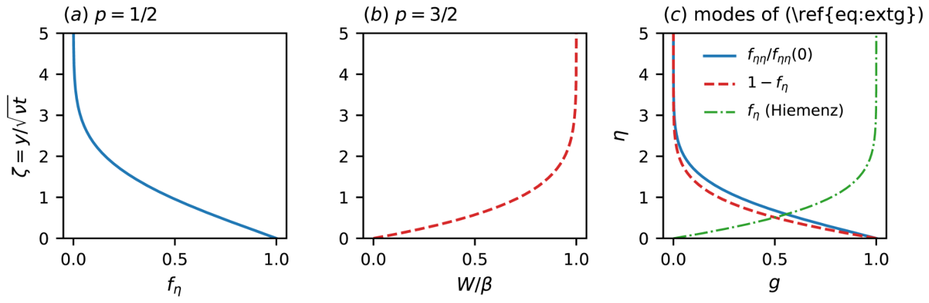
Table 4.
Values of the exact profiles of Figure 1. The Hiemenz function used in the last two columns has .
Table 4.
Values of the exact profiles of Figure 1. The Hiemenz function used in the last two columns has .
| or | ||||
|---|---|---|---|---|
| wall slope |
The three branches thus divide cleanly. Both and satisfy (76) and are exact solutions of the full equations, in elementary functions, with : they are respectively the flow driven by wall motion at constant velocity and the flow driven by a constant pressure gradient. The branch satisfies neither the outer condition nor (76).
9.2. The Stagnation-Point Family: An Exact Unsteady Reduction
The case of Section 7.2 is stated separately because it furnishes an exact reduction of the full Navier–Stokes system that is genuinely unsteady, in the sense that no -derivative is discarded and none is forced to vanish.
Here , , ; normalising gives and
Since , the memory term of (3) vanishes identically and, since , so do the groups of (35) and (40). The velocity field is
with v independent of x, so identically. The full system reduces without approximation to
subject to , , together with the transverse balance, which from (41) with , collapses to
We have verified both against the physical equations (Appendix D). Equation (91) is the unsteady stagnation-point equation, whose steady limit is the Hiemenz solution [16]; the class is among those identified in [20] as satisfying the full equations. Note that (91) is first order in and parabolic, with no degeneracy anywhere: unlike the channel family of Section 7.3, this reduction is an evolution problem in , and may be integrated forward from data at . The reason is visible in Section 7.4: the elliptic contribution to the symbol carries the factor , which is identically zero here.
9.3. The Gauge Mode
Finally, a one-parameter family of solutions exists for every . Adding a function of alone, , changes only the terms and in (3), which cancel provided , that is
The same shift leaves invariant, since reproduces exactly, so the velocity field is unchanged: the mode is pure gauge, corresponding to the freedom in the additive constant of . Its exponent is the one that appears in the wall condition (57), which is not a coincidence—the gauge freedom is exactly what impermeability leaves undetermined—and it accounts for the term that arises in closed-form solutions of the case , .
9.4. The Steady Limit of the Channel Family
The reduced system (60)–(61) is nonlinear, fourth order and elliptic, and we do not expect it to be integrable. Its steady limit, however, is. We emphasise at the outset that the solution obtained below is not new: it is the classical Jeffery–Hamel solution [14,18], one of the small number of known exact solutions of the Navier–Stokes equations, given in elliptic-function form by Rosenhead [27] and treated in the standard texts [4,19]. Sun [32] points to the same literature for this configuration. What is recorded here is the route: the identification is a consequence of the closure condition , it is obtained from the full transformed system with no term discarded, and it therefore serves as an independent check on the reduction and fixes the geometry of the unsteady problem.
9.4.1. The Steady Reduction
Set , so that and , . In (61) the two convective contributions and cancel identically, and . The system therefore collapses to the fourth-order ordinary differential system
9.4.2. Reduction to the Jeffery–Hamel Equation
Equations (94)–(95) are integrable in closed form. Substituting
the whole system reduces to an exact derivative,
so that, with ,
Equation (98) is the Jeffery–Hamel equation [14,18]. Multiplying by and integrating once more,
a cubic in v, so that v is a Weierstrass ℘ function of , equivalently a Jacobi elliptic function [11,19,27]; the large-Reynolds-number form of the converging case is due to Pohlhausen [24]. The constants , and the two constants of integration are fixed by (57), (59) and the volume flux.
That (96) should work is clear in retrospect. For one has , so with ; the stream function is a function of the polar angle alone, which is the defining form of Jeffery–Hamel flow. The steady limit of the case is therefore not merely similar to Jeffery–Hamel flow but identical with it.
9.4.3. Consequences
Three points follow.
First, this is an end-to-end validation of the reduction. A known exact solution of the Navier–Stokes equations is recovered from the transformed system with every term retained and no thin-layer assumption made anywhere; the value of the calculation lies in the check, not in the solution. Had any of the operators S, or the groups of (52) been in error, (97) would not be an exact derivative and (98) would not appear.
Second, it settles the geometry. The Jeffery–Hamel problem is posed between two plane walls, that is between two surfaces of constant and hence of constant . This is the origin of the channel domain adopted in Section 8.2, and it explains why the half-plane condition is inappropriate for : there is no outer region, and the vorticity (58) is not required to decay because the flow is rotational throughout.
Third, it supplies the natural reference state for the unsteady problem. Equation (98) inherits the full structure of Jeffery–Hamel flow, including the non-uniqueness of its solutions above a critical value of and the associated bifurcations [2,11]. Any unsteady solution of (60)–(61) that is -independent must be one of these; and since the problem of Section 8.3 requires data at as well as at , the Jeffery–Hamel states are the obvious candidates for that condition. Whether the resulting boundary-value problem possesses solutions, and whether they depend sensitively on T, is the natural next question and is left for a separate study.
10. Solutions of the Unsteady Stagnation-Point Equation
Of the two reductions of the full system identified in Section 7.2, the case is the one that can be solved. Equation (91),
has , so by Section 7.4 it is parabolic and first order in , and the initial-value problem is well posed. We first show that it admits no closed-form similarity solution compatible with a fixed wall, and then solve it.
10.1. The Point Symmetries, and a No-Go Statement
Equation (100) is autonomous in but admits no scaling group: under , , the four terms scale as , , and , and equality of the first three forces and then . The constant term—which is the pressure gradient —is what destroys the scaling; this is the precise sense in which the case of Section 9.1 is exceptional.
What remains is together with an infinite-dimensional family. Substituting into (100) changes the residual by exactly , so
is a symmetry for arbitrary , and these exhaust the point symmetries. The corresponding invariant reductions are the following.
(i) . The steady Hiemenz equation [16], which is itself not solvable in closed form; numerically.
(ii) . A travelling wave,
where F satisfies the steady Hiemenz equation; we have verified that the residual of (100) under (102) vanishes identically. This is (101) with . It is an exact unsteady solution, but cannot vanish for all unless : the wall condition fails. Since , the solution describes a wall moving normal to itself, or equivalently uniform transpiration, rather than a fixed impermeable surface.
(iii) . The invariants are and , giving ; substitution reduces (100) to , so no solution exists on this orbit.
Hence:
Proposition 4.
The only group-invariant solution of (100) satisfying is the steady Hiemenz solution.
No closed-form unsteady similarity solution of the fixed-wall problem exists within the point symmetries. This is a genuine obstruction, and it stands in contrast to the case of Section 9.1.1, where the absence of the constant term restores enough symmetry for the -invariant ansatz to close and for the solution to be written in elementary functions.
10.2. Numerical Solution
Because (100) is parabolic it may be integrated in . Writing and ,
which we solve from the impulsive start , , by second-order central differences in and a backward-Euler step in , with Newton iteration on the resulting tridiagonal system and the integral f evaluated by the trapezoidal rule. The results reported below use with 3000 intervals; the short-time behaviour was checked separately on –1 with up to intervals, and is grid-converged to four Figures.
Long time. As the computation gives
which reproduces the Hiemenz value to six Figures. This is an independent check on the reduction: the steady limit of the unsteady transformed equation is the correct steady exact solution of the Navier–Stokes equations.
Short time. As the computed wall shear follows
the ratio taking the grid-converged values and at and . This law is not fitted: it is the wall shear of the exact solution (79) of Section 9.1.1, for which in magnitude. The two families of Section 9 are thus linked. At short time the constant term in (100)—the pressure gradient—has not yet acted, the equation degenerates to the form, and the flow is locally the Rayleigh–Stokes layer; the departure from (105) measures the onset of the stagnation-point straining. The crossover, where the two limits are comparable, occurs near .
11. Closed-Form Unsteady Solutions of the Full Equations
Section 10.1 showed that equation (100) admits no closed-form similarity solution compatible with a fixed wall. That conclusion is not a statement about the stagnation-point flow itself, however, but about the class of fields to which the similarity form (1) restricts us. Writing with forces throughout, and it is exactly this restriction that must be relaxed. Once it is, closed-form unsteady solutions of the full Navier–Stokes system exist and can be written down.
11.1. The Extended Ansatz and the Splitting
For , is constant and , are proportional to y and t; nothing then prevents the addition to of a term independent of x. We therefore take
so that, writing ,
The transverse velocity is unchanged and remains independent of x, so identically and (106) solves the full system with no approximation whatever, exactly as in Section 9.2.
Substituting (107) into (6b) with , and using , every term is either proportional to x or independent of it. The two groups must vanish separately, giving
The first is equation (100) unchanged. The second is new, and it is linear in g once f is known. We stress that no linearisation has been made: (109) is exact and holds for any f satisfying (108), the linearity being a property of the splitting by powers of x rather than of a small-amplitude assumption. What is particular about the solutions of Section 11.2 is only the choice of a steady f, which makes (109) separable. The transverse equation (92) is unaffected, since v does not involve g; the pressure is therefore insensitive to the added flow.
This splitting is the structural reason for the difference in tractability. The x-proportional part of the motion obeys a nonlinear equation with no useful symmetry, whereas the x-independent part obeys a linear one, for which superposition and transform methods are available.
11.2. Closed-Form Solutions
Take f to be the steady Hiemenz solution of (108). Then equation (109) has constant coefficients in and admits separable solutions with
Two members are elementary.
(i) The steady mode, . Differentiating the Hiemenz equation gives , which is (110) with and . Hence
normalised to , : the added velocity profile is proportional to the shear distribution of the Hiemenz flow. This is the solution of Rott [28].
(ii) The exponential mode, . Substituting into (110) gives
the first bracket vanishing by (108). The residual is therefore , which vanishes if and only if : the exponent is not free. Hence
is an exact solution, and in physical variables
with wall velocity . This is the solution obtained by Rott [28] for exponential acceleration of the plate.
The wall shear follows at once. For (114),
so the shear vanishes at the same station as the relative velocity between plate and fluid, which is not the case for the steady mode (111). For the latter the wall gradient is , using from (108); this reproduces the value of [28,36]. Both modes are plotted in Figure 1(c) and tabulated in Table 4.
11.3. Discussion
Three remarks place these solutions in context.
First, they are exact solutions of the Navier–Stokes equations, not of a thin-layer approximation to them. This is not a new claim—Rott states that the exact equations yield a soluble problem in this configuration, and Watson [36] likewise notes that the corresponding solutions satisfy the Navier–Stokes equations exactly—but those treatments, and the related oscillatory analysis of Glauert [12], reach them through boundary-layer reasoning and observe the exactness after the fact. In the present formulation the exactness is structural and visible from the start: is constant, , , and identically, so no term is ever discarded.
Second, the no-go result of Section 10.1 is corroborated independently. Rott [28] remarks that when the f-flow itself is unsteady a term enters the nonlinear equation, so that solutions can be obtained only to a linearised approximation. That is precisely equation (100), and precisely our conclusion, reached here from the point symmetries rather than from the failure of a method. The two statements are complementary: Section 10.1 explains why no closed form is available, and Section 10.2 supplies the solution that must therefore be obtained numerically.
Third, the linearity of (109) makes the general problem tractable. For an arbitrary prescribed wall velocity the equation may be solved by Laplace transform, as Watson [36] showed, giving small- and large-time expansions in terms of the wall motion; for impulsive motion he finds a settling time in terms of the undisturbed displacement thickness. Equations (111) and (113) are the two cases for which the transform inverts in closed form. Together with the numerical solution of Section 10.2 for the nonlinear part, they give a complete description of the extended family (106): the x-proportional motion evolves from the Rayleigh–Stokes law to the Hiemenz state, while the x-independent motion is governed by a linear equation with the elementary solutions above.
12. The Unsteady Channel Problem
The case is the one for which the transformation reduces the full Navier–Stokes system with the streamwise-diffusion operators retained and finite, and it is therefore the case in which the elliptic character established in Section 7.4 has consequences. We solve it here. The question the computation is designed to answer is the one left open in Section 8.3: since the reduced problem requires data at as well as at , how strongly does the solution depend on that terminal condition?
12.1. Formulation and Method
The geometry is sketched in Figure 3. With , and , the reduced system is the pair (60)–(61) on the rectangle , . Written out,
The data are those of Section 8.3: , at and , at ; prescribed at ; and f and prescribed at . Note that (116) degenerates at to , consistent with lying in for that equation, so no condition on f is imposed there.
We take , , , and as terminal data the steady Jeffery–Hamel solution of Section 9.4, obtained from (94)–(95) with the same wall conditions; it has and is free of reverse flow at this . At we set , an irrotational start: the flow begins as the potential source flow in the wedge, for which and the wall is a slip surface, and no slip is enforced only for .
Equations (116)–(117) are discretised by second-order central differences on a uniform grid and solved by Newton’s method with an exact Jacobian and a line search, using Woods’ second-order formula for the wall vorticity and continuation in the initial data from the steady state. Two checks were made. With steady data at both and the computation reproduces the steady solution to within discretisation error, on a grid. And the wall vorticity at takes the values , and on grids of 16, 24 and 32 intervals, so the results below are grid-converged to five Figures.
12.2. Relaxation from the Irrotational Start
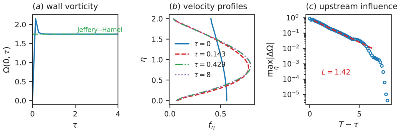
Figure 5(a) shows the wall vorticity . From at it rises steeply, overshoots slightly near , and settles on the Jeffery–Hamel value:
against the steady value . The relaxation is therefore complete to four Figures by , that is after one diffusion time . Figure 5(b) shows the corresponding velocity profiles: the initial slip profile is replaced within by the Jeffery–Hamel profile, the adjustment being confined to a layer near the walls at the earliest times and spreading across the channel as grows.
12.3. Upstream Influence of the Terminal Condition
The substantive question is how far the terminal data propagate. We therefore solved the problem twice with identical data except for the terminal vorticity, taking and , and measured . The result, Figure 5(c), is an exponential decay backwards in ,
over more than three decades. A change in the terminal vorticity alters the solution by at , by at , and not at all at , where is prescribed.
This is the physical content of the ellipticity, and it is a reassuring result. The reduced problem is genuinely a boundary-value problem in and cannot be marched; but the influence of the terminal condition is localised, with an e-folding length of about in , comparable to the relaxation time of Section 12 B. Two consequences follow. First, a solution computed on is independent of the choice of terminal data over the range , so the non-uniqueness implied by the free terminal condition—including the choice among Jeffery–Hamel branches above the critical Reynolds number—does not contaminate the early evolution. Second, the parabolic marching that the truncated system (3) licenses is justified a posteriori at this Reynolds number, in the sense that it agrees with the elliptic solution except within a few units of of the terminal boundary. The singular limit of Section 7.4 is thus singular in structure but mild in effect: the upstream influence it introduces is exponentially confined rather than global.
12.4. What Sets the Influence Length
Equation (119) was obtained at one Reynolds number, and the elliptic terms carry the factor , so the obvious expectation is that L should shrink as grows and the system approaches the parabolic limit. We tested this by repeating the computation over at two channel widths, and 2, with throughout. The results are shown in Figure 4(a) and tabulated in Table 6.
The expectation is met, but not for the expected reason. At fixed the influence length falls roughly as ; at fixed it grows in proportion to . Both dependences are the same statement seen edge on, because the physical half-angle of the wedge is
the walls being surfaces of constant . Plotted against , Figure 4(b), the two families collapse onto
with and a spread of over the resolved set. The collapse was checked directly on matched pairs, that is on chosen to give the same from different Reynolds numbers: against gives against , and against gives against , in each case a factor of four in for a change in L. These pairs are the triangles in Figure 4(b). Refining the grid does not remove the residual , which is a weak genuine dependence, , that we have not pursued. The open symbols in Figure 4 are runs at the highest for each width, where the wall layers are no longer resolved on the fixed grid and L flattens spuriously; they are excluded from the fit.
12.5. Robustness, and What the Prefactor Depends On
Three checks bear on how far (121) can be pushed.
The prefactor is not universal. Reversing the flow changes it. Repeating the computation with , a converging channel, at , gives against for the diverging case at the same , that is rather than , a difference of . The two configurations have different steady states—the converging wedge has against —and there is no reason for the prefactor to be shared. What survives the reversal is the scaling: L is still set by the geometry. The collapse (121) should therefore be read as a statement about how L varies with at fixed sense of flow, with a prefactor of order two that must be determined case by case.
L does not depend on the size of the terminal perturbation. Repeating the measurement with the terminal vorticity scaled by and by instead of gives and against : a variation of for a fivefold change in the perturbation. The decay rate is thus a property of the linearisation of the operator about the solution, not of the disturbance, which is what (119) claims but does not by itself establish.
The residual dependence is not a grid effect. Halving h changes L by less than and leaves the difference within a matched pair intact, so is not discretisation error. Whether it is a genuine weak dependence or an artefact of holding T fixed while varies we have not determined; resolving it would require runs at several T for each , which we have not attempted. All results quoted here are at a single flux .
12.6. Consequence
The consequence is the main point of this paper. The upstream influence introduced by streamwise diffusion is controlled by the geometry, not by the viscosity. It does not disappear at high Reynolds number, as one would expect of a viscous correction, but it does disappear for a slender channel, , at any Reynolds number whatever. In that limit the elliptic problem degenerates to the parabolic one and the marching that the truncated system licenses is exact in the limit. Conversely, for a wide channel the influence length is in and marching carries an error that no reduction of viscosity will remove.
The mechanism is visible in the coefficients of (117). The diffusion of in the direction has coefficient , while the advection has coefficient , dominated at large by . Their ratio is the classical upstream-influence length of an advection–diffusion balance,
and since and carry the weights 2 and 1 under , the combination that is invariant under the scaling is , which is at the wall. Equation (122) therefore predicts a collapse on , as observed, with a prefactor of order unity.
Figure 5.
The unsteady channel problem, , , , , started irrotationally. (a) Wall vorticity ; the dotted line is the steady Jeffery–Hamel value . (b) Velocity profiles at , , 1 and T. (c) Upstream influence of the terminal condition: the change produced by raising by , against , with the fit (119).
Figure 5.
The unsteady channel problem, , , , , started irrotationally. (a) Wall vorticity ; the dotted line is the steady Jeffery–Hamel value . (b) Velocity profiles at , , 1 and T. (c) Upstream influence of the terminal condition: the change produced by raising by , against , with the fit (119).
13. Conclusions
Applying the diffusion-time-scale transformation (1) to the full two-dimensional incompressible Navier–Stokes system, and retaining every term, yields
with and . Continuity is satisfied identically, and the transverse momentum equation reduces to the compact closed form (41), whose unsteady contributions carry the weights and whose wall value agrees with the exact identity .
The main conclusions are these. (i) The transformation reduces the full system to two independent variables if and only if or , equivalently or ; for every other member of the family the reduction is of the truncated system only. (i′) Exact unsteady solutions follow from the -invariant ansatz , which closes if and only if and ; the branch gives in elementary functions, exact for the full equations and satisfying every imposed condition at all , while cannot meet the outer condition. The case gives the exact unsteady reduction , which is parabolic and may be marched in . (i″) That equation admits no closed-form similarity solution compatible with a fixed wall: its point symmetries are together with , and the only invariant solution meeting the wall conditions is the steady one. Integrated numerically it gives , the Hiemenz value, as and as , the latter being the wall shear of the exact solution (79). (i′′′) Relaxing by adding an x-independent term to splits the problem into equation (100) and the linear companion (109), whose elementary solutions (111) and (113) are closed-form unsteady solutions of the full equations; they coincide with those of Rott [28] and Watson [36], obtained there by boundary-layer reasoning and here directly, with no term discarded. (ii) Even in the reducible case the resulting equation is elliptic in , with principal symbol , degenerate only on ; is therefore not an evolution variable and the limit is singular. (iii) On the degenerate boundary the Fichera function is for the vorticity equation and 0 for the equation defining the vorticity, so exactly one condition may be imposed at , on and not on f, while data are required at as well. (iv) For the truncated system the characteristic direction reverses across , the locus of [32] in the limit ; the operator is regular there, but no marching direction exists across it. (v) The steady limit of the system integrates exactly to the Jeffery–Hamel equation; the solution is classical, but its recovery from the full transformed system with nothing discarded is an independent check on the reduction, and it fixes the natural domain as a channel . (vi) The assumption is not consistent with the motion described by the reduced equation. (vii) Impermeability requires , which explains the structure encountered in the closed-form solutions of Sun [32]. (viii) Solved as the boundary-value problem it is, the system relaxes from an irrotational start onto Jeffery–Hamel flow within , and the terminal data influence the solution only over a length L in , decaying exponentially backwards. (ix) That length collapses on the wedge half-angle, , to within over a factor of 16 in Reynolds number, with a prefactor that depends on the sense of the flow ( for a converging wedge against for a diverging one) but a scaling that does not.
The last of these is the result we would emphasise. The upstream influence that streamwise diffusion introduces into a similarity reduction is geometric rather than viscous: it is fixed by the divergence angle of the channel and is essentially independent of . It therefore does not disappear at high Reynolds number, as a viscous correction would, but it does disappear for a slender channel at any Reynolds number. Marching in the similarity time is consistent in slender geometries however inviscid, and inconsistent in wide ones however viscous. The weak residual dependence , the behaviour at angles approaching the Jeffery–Hamel bifurcation, and the corresponding question for three-dimensional reductions are left for future work.
Author Contributions
Bo Hua Sun: Conceptualization, Methodology, Formulations, Formal analysis, Funding acquisition, Investigation, Writing- Original draft preparation, Writing- Reviewing and Editing and all relevant works.
Data Availability Statement
The data supporting the findings of this study are available from the corresponding author upon reasonable request.
Acknowledgments
My investigations into the boundary layers started from my tenure as a professor at the Cape Peninsula University of Technology (CPUT), South Africa. I am profoundly grateful to CPUT for granting me complete academic autonomy to advance this research agenda. This vital institutional support laid the foundation for the principal conclusions presented in this manuscript. I also extend my deepest gratitude to former Vice-Chancellor (now Chancellor) Prof. Brian Figaji, and former Deputy Vice-Chancellors Prof. J. A. Tromp and Prof. Anthony Staak, for their generous support and endorsement. Further academic support was provided by Xi’an University of Architecture and Technology (XAUAT) and the Beijing Institute of Nanoenergy and Nanosystems (BINN), Chinese Academy of Sciences. I sincerely thank former XAUAT President Prof. Xiao-Jun Liu and current President Prof. Xiang-Mo Zhao, along with BINN Founding Director Prof. Zhong Lin Wang, for their unwavering encouragement and invaluable resource support throughout this study.
Conflicts of Interest
The authors declare that there are no competing financial interests.
Appendix A. Identities for the Stretching Operator
With ,
so and are eigenfunctions of with weights 1 and 2. Explicitly,
The integral curves of are the rays , along which reduces to a directional derivative; this is the geometric origin of the degeneracy of the symbol in Section 7.4. The third relation, obtained by induction from the commutator, is what permits the streamwise-diffusion groups to be written alternately as or as .
Appendix B. Coefficient Dictionary
Given with and :
The parameter is singular in the single case (), for which and ; the operators S and then vanish identically and does not appear. Everywhere else . The operators appearing in the text follow from (14) with the exponent q of the relevant prefactor:
| quantity | prefactor | q | operator |
| U | m | ||
Appendix C. Cancellations in the Transverse Equation
Write , so and
Expanding the four convective and diffusive groups of (40) and substituting for from (35) produces the pairwise cancellations of Table A1; the surviving terms are those of (41).
Appendix D. Verification Protocol
Every transformed relation quoted above was checked by two independent routes.
(a) Symbolic. Equation (41) was verified by computer algebra: forming the difference between (40) and (41) for a general and general with , and substituting for from (35), leaves a residual equal to times the residual of (35), hence zero on solutions.
(b) Numerical, in physical variables. For a prescribed analytic test profile and prescribed , C, the stream function was formed as an explicit function of , and and were evaluated from (6b) and (6c). The scaled quantities and were then compared with the right-hand sides of (35) and (40) at an arbitrary interior point. Agreement to machine precision was obtained for , and . The same procedure applied to (8), term by term in , , and with , confirms (53) for and exhibits, for , a discrepancy in precisely those terms containing , equal to the contribution of . This is the numerical counterpart of the closure condition of Section 7.
(c) Boundary classification. The coefficient matrix (62), its divergence, and the Fichera functions (66) were computed by the same algebra system, and equation (68) was verified for general by forming directly from in physical variables. The convention in (63) was checked against the heat operator as stated in the text.
(d) Exact solutions. The residual of (3) under (79) with was evaluated symbolically and vanishes identically, as do (hence V) and ; the three conditions (80) were checked by direct limits. The three-group decomposition (75) was obtained by substituting (73) and collecting powers of . For the case , P and computed from the physical equations agree with (91) and (92).
(e) Equation (100). The symmetry family (101) and the travelling wave (102) were checked symbolically; the residual difference under is , and that of (102) vanishes. The solver of Section 10.2 was verified against the Hiemenz value and refined on three grids.
(f) Extended family. The splitting of (106) into (108) and (109) was obtained by collecting powers of x in the physical x-momentum equation. Both (111) and (113) were verified by substitution into (109) with all derivatives of f above second order reduced by (108); the residual of is , fixing .
(g) Channel computation. The solver of Section 12 was validated by supplying steady data at both and , which reproduces the steady solution to discretisation accuracy, and by grid refinement on 16, 24 and 32 intervals. Newton residuals were reduced to or below in all runs reported. The collapse (121) was tested on matched pairs at fixed grid spacing , and again after halving h, which changes L by less than and does not remove the difference within a pair. The independence of L from the amplitude of the terminal perturbation was checked by repeating the measurement at three amplitudes, giving , and for terminal vorticity scaled by , and .
References
- Abramowitz, M.; Stegun, I. A. <italic>Handbook of Mathematical Functions</italic>. Dover; 1972. [Google Scholar]
- Banks, W. H. H.; Drazin, P. G.; Zaturska, M. B. On perturbations of Jeffery–CHamel flow. J. Fluid Mech. 1988, 186, 559–C581. [Google Scholar] [CrossRef]
- Barenblatt, G. I. Scaling, Self-Similarity, and Intermediate Asymptotics; Cambridge University Press, 1996. [Google Scholar]
- Batchelor, G. K. An Introduction to Fluid Dynamics; Cambridge University Press, 1967. [Google Scholar]
- Blasius, H. Grenzschichten in Fl—-ssigkeiten mit kleiner Reibung. Z. Math. Phys. 1908, 56, 1–C37. [Google Scholar]
- Bluman, G. W.; Kumei, S. Symmetries and Differential Equations; Springer, 1989. [Google Scholar]
- Buckingham, E. On physically similar systems: illustrations of the use of dimensional equations. Phys. Rev. 1914, 4, 345–C376. [Google Scholar] [CrossRef]
- Dennis, S. C. R. The motion of a viscous fluid past an impulsively started semi-infinite flat plate. J. Inst. Maths Applics 1972, 10, 105–C117. [Google Scholar] [CrossRef]
- Falkner, V. M.; Skan, S. W. Some approximate solutions of the boundary layer equations. Phil. Mag. 1931, 12, 865–C896. [Google Scholar] [CrossRef]
- Fichera, G. Sulle equazioni differenziali lineari ellittico-paraboliche del secondo ordine. Atti Accad. Naz. Lincei Mem. Cl. Sci. Fis. Mat. Natur. Sez. 1956, 5, 1–C30. [Google Scholar]
- Fraenkel, L. E. Laminar flow in symmetrical channels with slightly curved walls. I. On the Jeffery–CHamel solutions for flow between plane walls. Proc. R. Soc. Lond. A 1962, 267, 119–C138. [Google Scholar] [CrossRef]
- Glauert, M. B. The laminar boundary layer on oscillating plates and cylinders. J. Fluid Mech. 1956, 1, 97–C110. [Google Scholar] [CrossRef]
- Hall, M. G. The boundary layer over an impulsively started flat plate. Proc. R. Soc. Lond. A 1969, 310, 401–C414. [Google Scholar] [CrossRef]
- Hamel, G. Spiralf?rmige Bewegungen z?her Fl—-ssigkeiten. Jber. Dt. Math.-Verein. 1917, 25, 34–C60. [Google Scholar]
- Hartree, D. R. On an equation occurring in Falkner and Skan’s approximate treatment of the equations of the boundary layer. Proc. Camb. Phil. Soc. 1937, 33, 223–C239. [Google Scholar] [CrossRef]
- Hiemenz, K. Die Grenzschicht an einem in den gleichf?rmigen Fl—-ssigkeitsstrom eingetauchten geraden Kreiszylinder. Dinglers Polytech. J. 1911, 326, 321. [Google Scholar]
- rmander, L. The Analysis of Linear Partial Differential Operators I, 2nd ed; Springer.
- Jeffery, G. B. The two-dimensional steady motion of a viscous fluid. Phil. Mag. 1915, 29, 455–C465. [Google Scholar] [CrossRef]
- Landau, L. D.; Lifshitz, E. M. Fluid Mechanics, 2nd edn; Butterworth–CHeinemann, 1987. [Google Scholar]
- Ma, P. K. H.; Hui, W. H. Similarity solutions of the two-dimensional unsteady boundary-layer equations. J. Fluid Mech. 1990, 216, 537–C559. [Google Scholar] [CrossRef]
- Oleĭnik, O. A.; Radkevič, E. V. Second Order Equations with Nonnegative Characteristic Form; Plenum, 1973. [Google Scholar]
- Olver, P. J. Applications of Lie Groups to Differential Equations, 2nd edn; Springer, 1993. [Google Scholar]
- Ovsiannikov, L. V. Group Analysis of Differential Equations; Academic Press, 1982. [Google Scholar]
- Pohlhausen, K. Zur nherungsweisen Integration der Differentialgleichung der laminaren Grenzschicht. Z. Angew. Math. Mech. 1921, 1, 252–C268. [Google Scholar] [CrossRef]
- Rayleigh, L. On the motion of solid bodies through viscous liquid. Phil. Mag. 1911, 21, 697–C711. [Google Scholar] [CrossRef]
- Riley, N. Unsteady laminar boundary layers. SIAM Rev. 1975, 17, 274–C297. [Google Scholar] [CrossRef]
- Rosenhead, L. The steady two-dimensional radial flow of viscous fluid between two inclined plane walls. Proc. R. Soc. Lond. A 1940, 175, 436–C467. [Google Scholar] [CrossRef]
- Rott, N. Unsteady viscous flow in the vicinity of a stagnation point. Q. Appl. Math. 1956, 13, 444–C451. [Google Scholar] [CrossRef]
- Stewartson, K. On the impulsive motion of a flat plate in a viscous fluid. Q. J. Mech. Appl. Math. 1951, 4, 182–C198. [Google Scholar] [CrossRef]
- Stokes, G. G. On the effect of the internal friction of fluids on the motion of pendulums. Trans. Camb. Phil. Soc. 1851, 9, 8–C106. [Google Scholar]
- Stuart, J. T. Laminar Boundary Layers; Rosenhead, L., Ed.; Clarendon Press; pp. 349–C408.
- Sun, B. H. Similarity solutions of a class of unsteady laminar boundary layer. Phys. Fluids 2024, 36, 083616. [Google Scholar] [CrossRef]
- Wang, C. Y. Exact solutions of the unsteady Navier–CStokes equations. Appl. Mech. Rev. 1989, 42, S269–CS282. [Google Scholar] [CrossRef]
- Wang, C. Y. Exact solutions of the steady-state Navier–CStokes equations. Annu. Rev. Fluid Mech. 1991, 23, 159–C177. [Google Scholar] [CrossRef]
- Wang, C. Y. Essential Analytic Laminar Flow; Springer Nature, 2024. [Google Scholar]
- Watson, J. The two-dimensional laminar flow near the stagnation point of a cylinder which has an arbitrary transverse motion. Q. J. Mech. Appl. Math. 1959, 12, 175–C190. [Google Scholar] [CrossRef]
Figure 2.
Wall shear from equation (103) (solid), compared with the short-time law (105) (dashed) and the steady Hiemenz value (dotted).
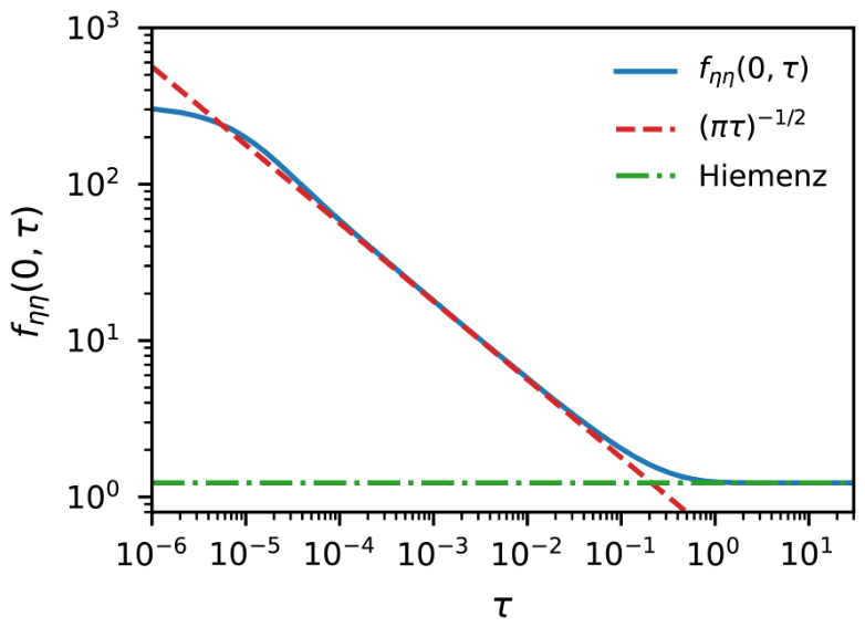
Figure 3.
Geometry of the numerical example. (a) The physical domain for : the walls are surfaces of constant with , so the flow occupies a wedge and measures angle. (b) The computational domain in with the data of Section 8.3. The line is characteristic and carries a single condition, on ; the other three sides are non-characteristic. The arrow marks the exponentially decaying upstream influence of the terminal condition, equation (119).
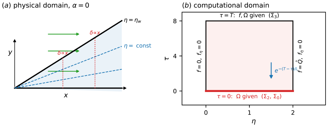
Figure 4.
The influence length. (a) L against Reynolds number at two channel widths; the lines are . (b) The same data against the wedge half-angle , collapsing onto . Triangles are the matched pairs of Section 12.4, which reach the same from Reynolds numbers differing by a factor of four. Open symbols are under-resolved and excluded from the fit.
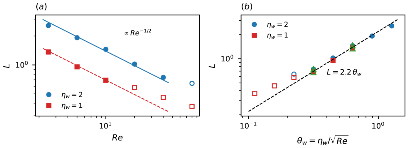
Table 1.
The two cases treated in [32], in Sun’s parameters and the derived quantities of Section 4. Only the second closes the full Navier–Stokes system.
| Section III of [32] | Section IV of [32], revised | |
|---|---|---|
| m | 0 | |
| 2 | 1 | |
| (varies) | const | |
| Closes full NS? | no | yes |
Table 3.
Fichera classification of the boundary of the rectangle for the reduced system (60)–(61) with , and the resulting number of admissible conditions. The last column gives the corresponding count for the truncated system ().
Table 3.
Fichera classification of the boundary of the rectangle for the reduced system (60)–(61) with , and the resulting number of admissible conditions. The last column gives the corresponding count for the truncated system ().
| Boundary | class | data (full) | data (truncated) |
|---|---|---|---|
| 2 (both on f) | 2 (both on f) | ||
| 2 (both on f) | 2 (both on f) | ||
| , | 1 (on ) | 1 (on ) | |
| 2 | 0 or 1 |
Disclaimer/Publisher’s Note: The statements, opinions and data contained in all publications are solely those of the individual author(s) and contributor(s) and not of MDPI and/or the editor(s). MDPI and/or the editor(s) disclaim responsibility for any injury to people or property resulting from any ideas, methods, instructions or products referred to in the content. |
© 2026 by the authors. Licensee MDPI, Basel, Switzerland. This article is an open access article distributed under the terms and conditions of the Creative Commons Attribution (CC BY) license (http://creativecommons.org/licenses/by/4.0/).
Copyright: This open access article is published under a Creative Commons CC BY 4.0 license, which permit the free download, distribution, and reuse, provided that the author and preprint are cited in any reuse.