

Submitted:
02 September 2026
Posted:
03 September 2026
You are already at the latest version
Abstract
Mobile social media applications generate substantial volumes of encrypted network traffic and can provide valuable evidence in digital forensic investigations. Although modern encryption protocols such as Transport Layer Security (TLS) and Quick UDP Internet Connections (QUIC) protect packet payloads, observable traffic characteristics remain available for application fingerprinting. This paper introduces a publicly available benchmark dataset comprising 25,116 encrypted bidirectional network flows collected from ten widely used Android social media applications across five independent capture days. An automated processing pipeline converts raw packet captures into structured flow-level representations while excluding leakage-prone attributes. Five tree-based classifiers: CatBoost, HistGradientBoosting, LightGBM, Random Forest, and XGBoost, are evaluated using a temporally separated protocol in which Days 1–4 are used for model development and Day 5 is reserved for final testing. A validation-only ablation evaluates aggregation windows of 1, 20, 40, 60, and 80 consecutive flows, selecting and locking a 60-flow window before Day 5 evaluation. On the held-out Day 5 test set, multi-flow classification substantially improves performance over the single-flow baseline across all five classifiers. XGBoost achieves the highest Macro F1-score at the locked 60-flow configuration, reaching 0.7317±0.0077, compared with 0.3155±0.0018 under single-flow classification. Post-hoc SHAP and LIME analyses further identify encrypted fingerprints, packet-size statistics, timing characteristics, protocol information, and directional traffic behavior as important contributors to application discrimination. The resulting dataset and reproducible evaluation framework provide a contemporary benchmark for studying encrypted mobile social media traffic under temporal separation and multi-flow inference.
Keywords:
benchmark dataset
; encrypted traffic analysis
; explainable artificial intelligence
; machine learning
; mobile social media
; network flow fingerprinting
; network security
1. Introduction
Mobile social media applications such as Facebook, Instagram, TikTok, WhatsApp, Telegram, YouTube, Reddit, Snapchat, Twitter, and LinkedIn have become integral to modern communication and generate substantial volumes of encrypted mobile network traffic. Beyond everyday communication, these applications can also provide useful evidence in criminal investigations, cyber incident response, and digital forensic examinations. When device artifacts are unavailable, deleted, or otherwise inaccessible, network traffic may provide supporting evidence for reconstructing application activity and communication patterns.
Modern mobile applications primarily rely on encryption protocols such as Transport Layer Security (TLS), Quick UDP Internet Connections (QUIC), and end-to-end encryption to protect communication confidentiality [1]. Although encryption prevents direct inspection of network payloads, it does not completely conceal communication behavior. Observable characteristics such as packet timing, flow duration, packet-size distributions, transport-layer behavior, and encrypted-session fingerprints remain available for analysis. Previous studies have shown that such characteristics can be used to distinguish applications without decrypting network traffic [2,3]. From a digital forensic perspective, encrypted network flows may therefore serve as supporting artifacts for identifying application-related network activity when payload contents are unavailable.
Despite growing interest in encrypted traffic fingerprinting, publicly available datasets specifically designed for mobile social media application identification remain limited. Existing studies often rely on proprietary datasets, different traffic environments, or evaluation procedures that make direct comparison and reproducibility difficult. In addition, performance obtained from randomly partitioned network flows may not reflect how a classifier behaves when applied to traffic collected during a later capture session.
To address these limitations, this study constructs and publicly releases a benchmark dataset for encrypted mobile social media traffic fingerprinting. The dataset contains traffic from ten widely used applications collected across five independent capture days and is accompanied by a reproducible processing pipeline for converting packet captures into labeled flow-level representations. The benchmark is evaluated using a temporally separated protocol in which Days 1–4 are used for model development, and Day 5 is reserved for final testing.
The main contributions of this work are as follows:
- We construct a publicly available benchmark dataset containing 25,116 encrypted mobile network flows from ten widely used social media applications collected across five independent capture days.
- We provide a reproducible packet-capture processing and preprocessing pipeline that transforms raw traffic into flow-level statistical representations while excluding leakage-prone attributes from model training.
- We evaluate five competitive tree-based classifiers using a temporally separated protocol in which Days 1–4 are used for model development, and an unseen Day 5 capture is reserved for final testing.
- We conduct a validation-only multi-flow ablation using window sizes of 1, 20, 40, 60, and 80 flows and select a common 60-flow operating window before accessing the final Day 5 results.
- We compare conventional single-flow classification with the locked 60-flow configuration on the temporally held-out Day 5 test set to quantify the value of aggregating evidence across consecutive encrypted flows.
- We apply SHAP and LIME to the highest-performing Day 5 classifier and evaluate SHAP–LIME agreement to examine the flow characteristics associated with application discrimination.
- We publicly archive the benchmark dataset through Mendeley Data [4] and provide the accompanying implementation and processing resources to support reproducibility and future comparative research.
The remainder of this paper is organized as follows. Section II reviews related work. Section III describes the dataset construction process. Section IV presents the methodology and experimental protocol. Section V reports the classification results, including the validation-based multi-flow ablation and temporally held-out Day 5 evaluation. Section VI presents the SHAP and LIME analyses. Section VII discusses the findings and their practical implications. Section VIII presents the limitations of the study. Finally, Section IX concludes the paper and outlines directions for future work.
2. Related Work
Encrypted traffic analysis has emerged as an active research area spanning traffic classification, anomaly detection, privacy analysis, asset identification, and cybersecurity monitoring. Shen et al. survey machine learning approaches for encrypted traffic analysis across traffic characterization, malicious activity detection, and user behavior inference [5]. Agrawal et al. similarly show that encrypted mobile traffic can reveal application usage, device behavior, and user activity through observable flow characteristics [6]. Together, these studies establish encrypted metadata as an important source of operational and forensic information when packet payloads are inaccessible.
Application fingerprinting seeks to infer application identities from encrypted traffic without inspecting payload contents. Early approaches relied on transport metadata, DNS information, packet statistics, and temporal correlations. He et al. showed that encrypted mobile applications retain distinguishable behavioral signatures despite payload encryption [7]. Fernandez-Terrasa et al. demonstrated that JA4+ TLS fingerprints remain useful for mobile application identification even as traditional metadata such as Server Name Indication (SNI) becomes less visible [8]. Yang et al. further showed that explicitly modeling packet size, direction, and inter-arrival time can improve fine-grained encrypted traffic classification [9].
Machine learning is widely used for encrypted traffic classification because it can capture complex relationships among observable traffic characteristics. Tree-based ensemble methods such as Random Forest and Gradient Boosting remain strong choices for structured flow-level data. Montieri et al. demonstrated the effectiveness of engineered flow-level features for encrypted mobile traffic classification [10]. Akbari et al. likewise showed that flow statistics, packet size, timing, and direction can support classification across HTTPS and QUIC traffic [11]. Their findings also demonstrated that classifiers may rely heavily on identifying TLS metadata such as SNI, emphasizing the importance of controlling leakage-prone attributes when evaluating encrypted application classification.
Multi-flow analysis has emerged as an alternative to treating every network flow as an independent classification instance. Chen et al. showed that single-flow classification may overlook relationships among related communications and proposed a “flow bunch” approach for multi-flow encrypted traffic classification [12]. Mengmeng et al. similarly demonstrated that relationships among multiple encrypted flows can improve application and behavior classification over isolated-flow approaches [13]. More recently, Wang et al. proposed MFSI, which represents multiple encrypted flows using a Multi-Flow Multi-Relational Graph and relational graph convolution to learn service-level traffic patterns [14]. These studies demonstrate the value of combining information from multiple flows and motivate further examination of how the amount of aggregated traffic context affects classification.
Explainable Artificial Intelligence (XAI) has also received increasing attention in network security, where predictive performance alone may provide limited insight into the characteristics responsible for model decisions. SHAP and LIME are widely used post-hoc techniques for examining feature contributions to machine learning predictions [15,16]. Recent forensic research has further demonstrated the complementary use of SHAP and LIME for examining feature relevance and model behavior [17]. Such analysis is particularly relevant to security and forensic applications because it allows analysts to examine the observable traffic characteristics associated with classification decisions rather than relying solely on predictive scores [18].
Reproducible research in encrypted mobile traffic classification is also constrained by the availability of suitable public datasets. Zhao et al. note that accurate application-level labeling and public release remain challenging because of privacy and traffic-collection requirements [19]. The MIRAGE dataset introduced by Montieri et al. provides an important public benchmark for mobile encrypted traffic classification [10], but it targets a broader collection of mobile applications rather than a benchmark specifically designed around social media applications. Mobile sensor forensic datasets [20] provide another source of mobile evidence but do not contain encrypted network-flow traffic for application fingerprinting. Previous encrypted traffic studies have also considered individual social media and messaging applications, but these applications are generally examined as subsets of broader application collections or under different traffic-classification objectives.
Despite these advances, the literature reviewed in this study does not provide a dedicated public benchmark that examines encrypted mobile social media applications in the same capacity considered here. In particular, limited attention has been given to a benchmark combining a social-media-specific application set, multi-day traffic collection, contemporary TLS/QUIC communication, leakage-controlled flow representations, temporal holdout evaluation, systematic multi-flow window analysis, and feature-level explanation within a single reproducible study. This distinction is important because social media applications frequently generate heterogeneous groups of encrypted connections for messaging, media delivery, advertisements, content retrieval, API communication, and background services, making their identification from isolated flows particularly challenging.
This study addresses this gap by constructing and publicly releasing a benchmark dataset containing encrypted network flows from ten widely used mobile social media applications collected across five independent capture days. Beyond dataset construction, the benchmark is used to examine how application discrimination changes when moving from isolated flows to consecutive-flow aggregation. In this way, the study provides both a reusable social-media-specific encrypted traffic dataset and a reproducible experimental baseline for evaluating application fingerprinting across capture sessions.
3. Benchmark Dataset Construction
This section describes the construction of the benchmark dataset used for encrypted mobile social media traffic fingerprinting. The dataset was designed to provide a reproducible collection of labeled, encrypted network flows suitable for machine-learning-based application fingerprinting and network traffic analysis.
3.1. Experimental Setup
Network traffic was collected using a controlled experimental environment consisting of an Android mobile device, a passive hardware network tap, and a dedicated monitoring workstation running Wireshark for packet capture. The Android device served as the traffic-generating endpoint and was used to interact with selected mobile social media applications under realistic usage conditions.
Internet connectivity between the mobile device and the broadband connection was routed through an ETAP-2003 passive network tap. The tap enabled packet-level monitoring without packet injection, modification, or active interference. A monitoring workstation connected to the tap’s monitor port captured raw network traffic in PCAP format using Wireshark. This passive architecture ensured transparent observation of traffic while preserving natural application behavior.
Figure 1 illustrates the experimental setup used for traffic capture.
3.2. Traffic Collection Protocol
Traffic collection focused on ten widely used social media applications: Facebook, Instagram, LinkedIn, Reddit, Snapchat, Telegram, TikTok, Twitter, WhatsApp, and YouTube. These applications were selected due to their widespread usage, diverse communication behavior, and increasing relevance in digital forensic investigations.
For each application, multiple traffic capture sessions were conducted across five collection periods to capture variability in user interaction and network conditions. During each session, realistic user activities were performed, including feed browsing, media streaming, content uploads, messaging, voice or video interactions where applicable, and application synchronization events. Traffic was collected separately for each application to ensure reliable label assignment during dataset construction.
3.3. Packet Capture and Flow Extraction
Captured network traces were stored in PCAP or PCAPNG format and processed using an automated Python-based pipeline based on NFStream. NFStream was selected because it provides efficient bidirectional flow generation together with rich statistical flow features suitable for network traffic analysis and machine learning applications [21]. The pipeline automatically identified all capture files in the input directory and extracted the application label and capture day from the filename. For example, filenames following the convention facebook_day1.pcapng and instagram_day3.pcapng were parsed to assign the application labels facebook and instagram and the capture-day identifiers day1 and day3, respectively.
Each packet capture was converted into bidirectional flow-level records using NFStream. NFStream was configured with statistical analysis, SPLT analysis, and up to 20 packet dissections using statistical_analysis=True, splt_analysis=True, and n_dissections=20. The resulting flow representation included statistical, temporal, packet-size, packet-inter-arrival-time, transport-layer, SPLT, and NFStream-derived application and protocol metadata.
Following flow extraction, three dataset metadata fields were added to each record: Label, capture_day, and capture_file. The Label field identifies the application associated with the controlled capture, capture_day identifies the collection day, and capture_file preserves the source capture filename. The Label field was repositioned as the first column, and each processed capture was exported as an individual CSV file.
3.4. Data Cleaning and Labeling
Application labels were assigned using the controlled data-collection procedure and capture-file naming convention rather than NFStream’s inferred application labels. Each capture file represented traffic collected during a controlled session for a designated social media application, and the corresponding application label and capture-day identifier were extracted automatically from the filename.
Importantly, the flow-extraction pipeline did not select or discard flows based on NFStream’s application_name field. All flows extracted from each controlled capture were retained at this stage. This avoids constructing the ground-truth dataset using the same application-identification information that could otherwise reveal the target class.
After extraction, the individual capture CSV files were grouped by application and concatenated to produce one merged CSV file per application. Schema consistency was checked during merging, while the application label was preserved as the first column. This resulted in ten application-level datasets corresponding to Facebook, Instagram, LinkedIn, Reddit, Snapchat, Telegram, TikTok, Twitter, WhatsApp, and YouTube.
3.5. Dataset Characteristics
Each application was captured across five independent collection days, producing 50 capture files that were subsequently processed with NFStream and merged by application into ten application-level CSV files. Although all applications were captured using the same collection protocol and approximately equivalent user interactions, the number of extracted bidirectional flows differs across applications. Because NFStream constructs flow records from the observed packet exchanges within each application session, the number of extracted flows depends on the characteristics of the captured traffic rather than the collection procedure itself [21]. Consequently, the resulting class imbalance reflects differences in the extracted network-flow records rather than inconsistencies in the data collection process. The final benchmark contains 25,116 labeled flow records, with the application-level distribution summarized in Table 1.
The extracted schema contains flow identifiers, endpoint and protocol metadata, bidirectional flow statistics, packet-size statistics, packet-inter-arrival-time statistics, transport-layer flag counts, SPLT sequence information, NFStream application metadata, and dataset metadata such as capture_day and capture_file. Application-level metadata extracted by NFStream was retained in the raw dataset at this stage but was subsequently treated separately during machine-learning feature preparation to prevent direct target leakage.
4. Methodology
This section describes the feature preparation, preprocessing, benchmark models, temporal evaluation strategy, multi-flow aggregation procedure, validation-based operating-point selection, training configuration, explainability analysis, and evaluation metrics used in this study.
4.1. Feature Selection and Preprocessing
Before model training, features that could introduce target leakage, capture-session memorization, or direct endpoint identification were removed. The complete list of excluded features and their corresponding removal categories is summarized in Table 2. These include the target label, capture metadata, NFStream application-identification outputs, endpoint identifiers, raw SPLT sequence fields, and absolute flow timestamps, all of which could leak application identity or capture-specific information into the learning process.
In particular, the NFStream application-identification fields and server-name information were removed because they may directly or indirectly reveal the target application. Likewise, source and destination endpoint identifiers were excluded to prevent models from memorizing capture-specific endpoints rather than learning generalizable encrypted traffic characteristics. Raw SPLT sequence fields and absolute timestamp attributes were also removed because they may encode collection-specific or temporal information that does not represent intrinsic application behavior.
After the predefined exclusions, infinite values were converted to missing values. Feature quality checks were then performed using the training partition only. Features containing exclusively missing values or having no variation in the training data were removed. This training-only procedure prevented information from the validation partition or held-out test day from influencing feature selection.
Numerical and categorical attributes were processed separately. Missing numerical values were replaced using median imputation, while missing categorical values were replaced using the most frequent category. To control categorical dimensionality, categories occurring fewer than ten times in the training data were mapped to a common __RARE__ category. Categorical variables were subsequently transformed using one-hot encoding, with previously unseen categories ignored during validation and testing.
All preprocessing transformations, including imputation, rare-category identification, categorical encoding, and training-based feature-quality filtering, were fitted exclusively on the training partition and then applied unchanged to the validation and held-out test data.
4.2. Benchmark Models
Five supervised machine-learning classifiers were evaluated: XGBoost, LightGBM, HistGradientBoosting, CatBoost, and Random Forest. These models were selected to provide representative tree-based ensemble and gradient-boosting approaches suited to heterogeneous tabular network-flow data. XGBoost and LightGBM provide scalable gradient-boosting implementations for large tabular datasets [22,23]. HistGradientBoosting implements histogram-based gradient boosting within the scikit-learn framework [24]. CatBoost uses ordered boosting to reduce prediction shift during training [25], while Random Forest was included as a robust bagging-based ensemble baseline [26].
The same leakage-controlled feature representation and preprocessing procedure were used for all five classifiers. The classifiers were trained at the individual-flow level; multi-flow aggregation was applied to their predicted class probabilities during validation and final testing rather than by retraining separate models on concatenated flow windows.
4.3. Temporal Development and Test Strategy
To evaluate generalization to traffic collected during an unseen period, a temporal holdout strategy was adopted. Capture Day 5 was reserved in its entirety as the final test set. Day 5 was not used to select the multi-flow window, select the focal model for explainability analysis, fit preprocessing transformations, or train the classifiers.
Data collected during Days 1–4 formed the model-development partition. Rather than randomly distributing individual flows between training and validation, each original capture file was first ordered according to its flow sequence. Within every Days 1–4 capture, the chronologically first 85% of flows were assigned to training and the final 15% were assigned to validation. The resulting structure was therefore
with
The contiguous within-capture split was used because the multi-flow analysis requires consecutive observations. A conventional random flow-level validation split would scatter flows from the same capture across training and validation and would disrupt the natural sequence required for constructing validation windows. The 85/15 split therefore preserves temporal ordering while ensuring that every development capture contributes observations to both training and validation.
The train-validation assignment was fixed for all experiments. Model training was repeated using five random seeds: 42, 123, 456, 789, and 2026. The seeds affected model stochasticity but did not alter which flows belonged to the training, validation, or Day 5 test partitions.
4.4. Multi-Flow Probability Aggregation
In addition to conventional single-flow classification, a multi-flow probability-aggregation strategy was evaluated to determine whether accumulating evidence from multiple consecutive encrypted flows improves mobile application identification.
The classifiers were trained exclusively at the individual-flow level. For an individual flow i, a trained classifier produces a probability vector over the application classes:
where denotes the predicted probability that flow i belongs to application class c.
For multi-flow inference, consecutive flows belonging to the same original capture file were ordered according to their original flow sequence and partitioned into non-overlapping windows. Windows were never permitted to cross capture-file boundaries. For a complete window containing W consecutive flows, the predicted class probabilities were averaged as
where represents the aggregated probability vector for the window.
The final application prediction was obtained as
Only complete windows were retained. Residual flows that could not form a complete window at the end of a capture were discarded. Because each capture file represented a controlled collection session for a single target application, each constructed window was additionally checked for label consistency.
4.5. Validation-Based Multi-Flow Window Selection
The number of flows used for multi-flow aggregation was treated as an operating parameter and selected exclusively from the validation partition. The candidate window sizes were
Here, represents the conventional single-flow condition, while progressively larger values quantify the effect of accumulating additional encrypted-flow evidence.
All candidate window sizes were evaluated on the fixed validation partition for each of the five classifiers and each of the five random seeds. For a model m and candidate window W, validation Macro-F1 was first averaged across the five seeds:
where represents the validation Macro-F1 obtained by model m at window size W using random seed s, and denotes the total number of random-seed runs. Thus, represents the mean validation performance of a particular model–window combination across the five seeds, reducing the influence of variation caused by a single random initialization or training run.
To avoid selecting a window that was optimized for only one classifier, a common validation score was subsequently calculated by averaging the seed-averaged Macro-F1 values across all five benchmark models:
where represents the number of benchmark classifiers. Here, measures the average validation Macro-F1 achieved by all five models at a given window size W. This provides a model-independent criterion for comparing the candidate window sizes rather than allowing the strongest result from a single classifier to determine the operating window.
The common operating window was then selected as
where denotes the candidate window size with the highest common validation Macro-F1. In other words, the selected operating window is the window that provides the strongest average validation performance across all five classifiers after accounting for variation across the five random seeds.
Once selected, was locked before final Day 5 performance was examined. This procedure separates operating-point selection from temporal test evaluation and prevents the held-out test day from influencing the choice of multi-flow configuration.
4.6. Final Held-Out Day Evaluation
Following validation-based selection, all five classifiers were evaluated on the held-out Day 5 data. Final testing was restricted to two predefined conditions:
The condition provides the single-flow baseline, while represents the validation-selected multi-flow operating point. Candidate window sizes that were not selected during validation were not used as final Day 5 operating points.
This design permits a direct comparison between conventional single-flow classification and the locked multi-flow strategy while preserving the independence of Day 5 from window selection. The same locked was applied to all five classifiers to ensure a common operating condition rather than selecting a separate test configuration for each model.
For both final conditions, performance was computed independently for each of the five random-seed runs and summarized using the mean and standard deviation. The number of complete evaluation windows was also recorded because larger values of W reduce the number of independent classification units.
4.7. Training Configuration
The benchmark models were configured using the hyperparameters summarized in Table 3. All five classifiers used the same fixed training, validation, and Day 5 test partitions and the same training-fitted preprocessing pipeline. The five random seeds were used to quantify variation attributable to model stochasticity rather than to generate alternative dataset partitions.
XGBoost, LightGBM, and CatBoost used the fixed external validation partition for early stopping. HistGradientBoosting instead used an internal 15% subset of the training partition solely for early stopping, while its reported validation performance and multi-flow window selection were computed using the same fixed external validation partition as the other models. Random Forest did not use early stopping.
4.8. Explainability Analysis
Post-hoc explainability analysis was performed using SHAP and LIME after completion of the final Day 5 evaluation. The model achieving the highest mean Macro-F1 across the five random-seed runs was selected as the focal model for explainability analysis.
The explainability stage was therefore conducted after model evaluation and did not influence model training, hyperparameter configuration, validation-based window selection, or the reported Day 5 performance. Its purpose was to characterize the feature-level behavior of the strongest final classifier under the locked multi-flow configuration.
For reproducible explanation generation, the selected model was refitted using seed 42 under the same preprocessing and training configuration. SHAP and LIME were then applied to correctly classified individual Day 5 flows. The explanations characterize the flow-level classifier that produces the probability vectors subsequently combined during multi-flow inference, rather than treating each aggregated window as a separately trained model.
For SHAP, up to 100 correctly classified Day 5 flows per application class were analyzed. Features were ranked according to their mean absolute SHAP values, and the 15 highest-ranked features were retained for each class.
For LIME, up to 25 correctly classified Day 5 flows per application class were explained using 3,000 perturbation samples per instance. Absolute local feature contributions were aggregated using zero-inclusive averaging, meaning that features not selected in a particular local explanation contributed a value of zero to the class-level average. The 15 highest-ranked features were retained for each application class.
Agreement between SHAP and LIME was examined using Jaccard similarity between their class-specific top-15 feature sets. Both exact agreement, based on individual encoded feature names, and semantic agreement, based on their underlying feature families, were evaluated to determine the extent to which the two explanation methods identified similar traffic characteristics.
4.9. Evaluation Metrics
Performance was evaluated using accuracy, macro-averaged precision, macro-averaged recall, Macro F1-score, Weighted F1-score, and multiclass log loss. Macro F1 served as the primary metric for validation-based operating-window selection because it gives equal importance to each application class irrespective of class frequency.
Macro F1 was computed as
where C is the number of application classes.
Weighted F1 was computed as
where is the number of observations belonging to class c and N is the total number of observations.
Multiclass log loss was additionally calculated from the predicted class probabilities:
where is an indicator equal to 1 when observation i belongs to class c, and is the predicted probability assigned to that class.
Validation performance was summarized across the five random-seed runs for every model and candidate window. Final Day 5 performance was reported only for the single-flow baseline () and the validation-selected common operating window (), using mean and standard deviation across the five seeds. Per-class precision, recall, and F1-scores and class-normalized confusion matrices were additionally used to examine application-specific behavior and systematic confusion between application classes.
5. Results
This section presents the experimental results obtained under the validation-controlled temporal evaluation protocol. Results are reported across five random seeds for the five benchmark models: CatBoost, HistGradientBoosting, LightGBM, Random Forest, and XGBoost.
Multi-flow window selection was performed exclusively on the validation partition derived from Days 1–4. Five candidate window sizes, , were evaluated, where represents conventional single-flow classification and larger windows aggregate the predicted probability distributions of consecutive flows from the same capture file. A single common operating window, , was selected using the mean validation Macro-F1 across the five benchmark models and five random-seed runs.
After selection, was locked before final evaluation on the temporally held-out Day 5 data. Consequently, the final Day 5 evaluation reports only two conditions for each model: the predefined single-flow baseline () and the validation-selected multi-flow configuration (). This separation ensures that the held-out Day 5 test set does not influence the selection of the multi-flow operating window.
5.1. Validation-Based Multi-Flow Ablation Results
Table 4 reports the multi-flow ablation results obtained on the validation partition for all five benchmark models and six candidate window sizes, . Results are reported as mean ± standard deviation across the five random-seed runs. The validation experiment was used exclusively to determine the common multi-flow operating window before evaluation on the held-out Day 5 test set.
The single-flow condition () produced relatively modest validation performance across all five classifiers, with mean Macro F1-scores ranging from for CatBoost to for XGBoost. Substantial improvement was observed when multiple consecutive flows were aggregated. At , Macro F1 increased to between and , demonstrating that combining evidence from multiple encrypted flows considerably improved application discrimination.
Performance improved further for several models at . Random Forest achieved the highest Macro F1 at this window with , followed by LightGBM with . The strongest and most consistent overall validation performance was observed at , where LightGBM and Random Forest both achieved a Macro F1 of , while CatBoost, HistGradientBoosting, and XGBoost also exceeded .
Increasing the aggregation window to did not provide further improvement. Macro F1 decreased across all five classifiers despite relatively high accuracy values. The evaluation at this larger window also contained only 14 complete validation windows, reducing class coverage and making aggregate accuracy less informative. These results indicate that the benefit of increasing multi-flow context peaked at approximately 60 consecutive flows under the validation setting.
To avoid selecting a window based on the performance of a single classifier, a common validation score was calculated by averaging the seed-averaged Macro F1 of all five models at each candidate window. The resulting common validation scores are summarized in Table 5.
The common validation Macro F1 reached its maximum at , with a score of . Consequently, the 60-flow configuration was selected as the common operating window:
This operating point was locked before final evaluation on the held-out Day 5 test set. The final temporal evaluation therefore compares the predefined single-flow baseline () against the validation-selected multi-flow configuration () for all five benchmark models.
5.2. Held-Out Day 5 Test Results
Following validation-based window selection, the locked multi-flow configuration () was evaluated on the temporally held-out Day 5 test set. No additional window-size selection or tuning was performed using Day 5. Final performance was therefore evaluated under only two conditions: the predefined single-flow baseline () and the validation-selected multi-flow configuration (). Figure 2 and Figure 3 compare the mean test accuracy and Macro F1-score, respectively, across the five random-seed runs.
Under the single-flow condition (), performance on the temporally held-out Day 5 data was relatively modest across all five classifiers. Accuracy ranged from for CatBoost to for LightGBM, while Macro F1 ranged from to . LightGBM achieved the strongest single-flow performance, with an accuracy of and a Macro F1-score of . These results demonstrate the difficulty of identifying mobile social media applications from individual encrypted network flows under temporal separation between the development and test data.
As shown in Figure 2 and Figure 3, applying the validation-selected 60-flow aggregation substantially improved performance for every classifier. Mean accuracy increased to between and , while Macro F1 increased to between and . Importantly, these improvements were obtained without retraining the classifiers for multi-flow inference; the same flow-level models were used, with their predicted probability distributions aggregated across consecutive Day 5 flows.
XGBoost achieved the highest Macro F1 at the locked operating point, increasing from under single-flow classification to . CatBoost produced a closely comparable Macro F1 of , compared with at . HistGradientBoosting increased from to , while LightGBM increased from to . Random Forest similarly improved from to .
For accuracy, LightGBM, Random Forest, and XGBoost each achieved a mean of at , compared with single-flow accuracies of , , and , respectively. CatBoost and HistGradientBoosting also exhibited substantial gains, reaching mean accuracies of and , respectively.
The consistent improvement across all five classifiers indicates that the observed benefit is not specific to a particular learning algorithm. Instead, the results support the central premise of the multi-flow approach: aggregating predictions across consecutive encrypted flows provides a more informative representation of application behavior than relying on isolated flows. Although performance on Day 5 remained below the corresponding validation results, the substantial improvement over the single-flow baseline demonstrates that the validation-selected operating point generalized to traffic collected during an unseen capture period.
5.3. Per-Class Performance
Detailed per-class results for all five models under the two final Day 5 evaluation conditions, the single-flow baseline () and the validation-selected multi-flow configuration (), are provided in Appendix A.1. The appendix reports the mean and standard deviation of precision, recall, and F1-score across the five random seeds for each of the ten application classes.
These per-class results complement the aggregate Day 5 performance presented in Figure 2 and Figure 3 by showing how classification performance varies across individual applications under single-flow and multi-flow inference. This class-level analysis is particularly important for interpreting the Macro F1-score, which assigns equal importance to each of the ten application classes and can therefore reveal class-specific differences that may not be apparent from overall accuracy alone. Comparing and also provides insight into which applications benefit most from aggregating evidence across multiple consecutive encrypted flows.
5.4. Confusion Matrix Analysis
To examine the class-specific effect of multi-flow aggregation, Figure 4 presents the class-normalized confusion matrices for XGBoost under the two final Day 5 evaluation conditions: the single-flow baseline () and the validation-selected multi-flow configuration (). XGBoost was selected for this detailed analysis because it achieved the highest Macro F1-score on the held-out Day 5 test set at the locked operating point.
The single-flow confusion matrix reveals substantial cross-application confusion on the temporally held-out Day 5 data. At , only Facebook and Reddit exceeded 50% class-specific recall, with diagonal rates of 60.1% and 58.7%, respectively. Several applications were considerably more difficult to identify from individual encrypted flows. Instagram, LinkedIn, Snapchat, WhatsApp, and YouTube achieved diagonal rates of only 21.8%, 19.5%, 20.3%, 22.7%, and 28.0%, respectively. Telegram, TikTok, and Twitter performed comparatively better, but their correct-classification rates remained below 50%.
The configuration substantially changed this pattern. Facebook, Reddit, Telegram, TikTok, and Twitter achieved 100% diagonal rates, while Snapchat and YouTube increased to 85.7% and 87.0%, respectively. Instagram improved from 21.8% at to 51.4% at , and LinkedIn increased from 19.5% to 57.1%. These changes show that aggregating evidence across consecutive encrypted flows substantially reduced the diffuse cross-application confusion observed under single-flow classification.
The improvement was particularly pronounced for applications that were difficult to distinguish from isolated flows. For example, Telegram increased from 38.0% to 100%, TikTok from 47.1% to 100%, Twitter from 46.2% to 100%, and YouTube from 28.0% to 87.0%. Snapchat similarly increased from 20.3% to 85.7%. Thus, the gain in aggregate Macro F1 at reflects improvements across multiple application classes rather than being driven by a single dominant class.
Despite these improvements, some class-specific ambiguity remained. WhatsApp was the most difficult application under the multi-flow configuration, with a diagonal rate of 31.2%. Its largest residual confusion was with Twitter (37.5%), followed by LinkedIn (14.6%) and Reddit (11.2%). Instagram also retained confusion with Facebook (25.7%) and Twitter (22.9%), while LinkedIn exhibited residual confusion with Instagram, Telegram, and WhatsApp (14.3% each). YouTube was predominantly identified correctly, although 8.7% of its windows were classified as WhatsApp and 4.3% as Twitter.
Overall, the confusion-matrix comparison demonstrates that the improvement from single-flow to multi-flow classification is associated with substantially stronger class separation for most applications. At the same time, the remaining errors, particularly those involving WhatsApp, Instagram, and LinkedIn, indicate that some encrypted application behaviors remain difficult to distinguish under temporal separation. These residual confusions provide a more nuanced interpretation of the Day 5 Macro F1 result and identify specific application pairs for which additional contextual information may be beneficial.
6. Explainable AI Analysis
Explainable AI analysis was performed using SHAP and LIME to examine the feature-level behavior of the highest-performing classifier in the final temporally held-out Day 5 evaluation. The operating window was first selected and locked at using only the Days 1–4 validation partition. All five classifiers were subsequently evaluated on the held-out Day 5 test set at the locked operating window, and the classifier achieving the highest mean Macro F1-score across the five random-seed runs was selected for post-hoc explainability analysis.
XGBoost achieved the highest Day 5 Macro F1-score at the locked configuration and was therefore selected as the focal model for SHAP and LIME analysis. Importantly, this post-hoc selection was used only to determine which final classifier to interpret. It did not influence model training, hyperparameter configuration, validation-based window selection, or the Day 5 predictions and performance measures reported in the primary classification evaluation.
6.1. SHAP Analysis
SHAP (SHapley Additive exPlanations) is a post-hoc explainability method based on game-theoretic principles that assigns feature-level contributions to model predictions [27].
SHAP was applied to the XGBoost classifier to identify the features contributing most strongly to its correctly classified predictions on the temporally held-out Day 5 test set. For each application class, mean absolute SHAP values were calculated across up to 100 correctly classified flows, and the 15 highest-ranked features were retained.
Table 6 presents the top-15 SHAP feature rankings for the ten application classes. The analysis provides a class-specific view of the network-flow characteristics associated with the model’s classification decisions. In particular, the rankings capture the relative influence of the statistical, protocol, timing, and encrypted fingerprint features represented in the feature space. Differences in the resulting rankings across application classes provide insight into the heterogeneous encrypted-traffic characteristics used by XGBoost when distinguishing mobile social media applications.
6.2. LIME Analysis
LIME (Local Interpretable Model-agnostic Explanations) is a post-hoc, model-agnostic explainability method that explains an individual prediction by approximating the behavior of a complex classifier with a simpler interpretable model in the local neighborhood of the instance [27].
LIME was applied to the XGBoost classifier as a complementary local explanation technique. For each application class, up to 25 correctly classified Day 5 flows were explained. The absolute local LIME weights were aggregated using zero-inclusive averaging, such that features not selected in a particular local explanation contributed a value of zero to the corresponding class-level average. Table 7 reports the 15 highest-ranked LIME features for each application class. The occurrence rate indicates the proportion of the analyzed local explanations in which each feature was selected.
The LIME results complement the SHAP findings, with packet-size statistics, directional traffic characteristics, timing information, protocol-related features, and encrypted client/server fingerprints appearing among the influential attributes across application classes. Differences in the exact rankings are expected because LIME explains model behavior around individual instances, whereas the reported SHAP rankings summarize feature contributions across multiple correctly classified flows. The recurrence of similar feature categories across the two methods provides complementary evidence about the encrypted traffic characteristics influencing XGBoost’s classification decisions.
6.3. SHAP–LIME Agreement
The consistency of the SHAP and LIME explanations was evaluated using Jaccard similarity between their respective top-15 feature sets. Two forms of agreement were calculated. Exact agreement compared the individual encoded feature names directly, whereas semantic agreement grouped encoded categorical variants under their original feature family. For example, different encoded values of client_fingerprint were treated as members of the common semantic feature client_fingerprint.
Figure 5 presents the class-level agreement results for the selected XGBoost model. The agreement varied across application classes, with semantic agreement generally exceeding exact agreement. Twitter exhibited the highest semantic agreement at 0.2000, followed by Telegram at approximately 0.1765 and TikTok at approximately 0.1667. Reddit and Twitter showed the highest exact agreement at approximately 0.1538. In contrast, Facebook and Instagram showed no exact feature overlap between their SHAP and LIME top-15 rankings, although Facebook retained some agreement after the features were grouped by semantic family.
The differences between exact and semantic agreement reflect the large number of encoded categorical fingerprint features used by the model. SHAP and LIME may identify different individual fingerprint values as important while still emphasizing the same underlying feature family. This is particularly visible for several application classes where semantic agreement exceeds exact agreement.
The relatively modest agreement between SHAP and LIME is also consistent with their different explanation mechanisms. SHAP assigns feature contributions using Shapley-value-based attribution, whereas LIME constructs local surrogate models around individual predictions. The two methods therefore do not necessarily select identical features even when explaining the same classifier. Their agreement at the semantic level provides additional evidence that both methods capture related categories of information used by XGBoost, particularly encrypted fingerprint attributes together with traffic, timing, and protocol characteristics.
7. Discussion
The primary novelty of this work is the construction of a new benchmark dataset for encrypted mobile social media traffic fingerprinting. Rather than relying on an existing network intrusion or general traffic dataset, traffic was collected specifically from ten widely used mobile social media applications across multiple capture sessions and transformed from raw packet captures into labeled flow-level records for application fingerprinting research. The resulting benchmark captures contemporary encrypted communication, including TLS- and QUIC-based traffic, while retaining statistical, directional, protocol, timing, and encrypted fingerprint information that can be examined without accessing application payloads.
The benchmark was also designed to reduce dependence on trivial application identifiers. Application labels, endpoint information, absolute timestamps, and other attributes capable of directly revealing the capture source were excluded from the predictive feature space. The temporal evaluation further strengthens this design: Days 1–4 were used for model development, while Day 5 remained unseen until final testing. Consequently, the reported test performance reflects application discrimination across capture sessions rather than performance obtained from a conventional random split of the complete dataset.
The experiments reveal an important characteristic of the new dataset. Individual encrypted flows provided limited evidence for distinguishing the ten applications, whereas combining consecutive flows produced substantially stronger application-level discrimination. The aggregation window was determined using only validation data from Days 1–4, where the 60-flow window was selected and locked before Day 5 testing. The improvement from the single-flow baseline to the locked multi-flow configuration on Day 5 suggests that application behavior is represented more effectively by sequences of encrypted communications than by isolated flows. This is relevant because a mobile application may generate multiple connections for content delivery, API communication, advertisements, media transfer, and background services.
The SHAP and LIME analyses provide further insight into the information captured by the benchmark. Application discrimination was associated with combinations of encrypted client/server fingerprints, packet-size statistics, timing characteristics, protocol information, and directional traffic behavior. Different applications relied on different combinations of these characteristics, suggesting that identification was not driven by a single universally dominant feature.
These findings also have practical relevance. Encrypted flow analysis could provide network administrators with additional visibility into mobile application activity without decrypting communication payloads. It could support identification of applications restricted by organizational policy, characterization of application-specific network usage, and retrospective analysis of historical network-flow records. In a forensic investigation, such classification could provide supporting evidence that network activity was consistent with a particular mobile application during a period of interest. It should not, however, be interpreted as evidence of specific user actions or communication content.
8. Limitations
Several limitations should be considered when interpreting the findings of this study.
First, the dataset was collected under controlled conditions using a single Android device and network environment. Although the temporally held-out Day 5 evaluation measures performance across capture sessions, all five capture days originated from the same experimental environment. Traffic characteristics may differ across devices, operating system versions, network providers, geographic locations, and routing conditions, and cross-environment generalization therefore remains to be evaluated.
Second, the dataset covers ten social media applications across five capture days. Application updates, changes in TLS/QUIC implementations, backend infrastructure, and content delivery networks may alter observable traffic characteristics over longer periods.
Third, the dataset contains some class imbalance. Macro-averaged metrics were therefore reported alongside accuracy and Weighted F1 to provide a balanced assessment of performance across the ten application classes.
Finally, multi-flow aggregation introduces a trade-off between additional traffic context and the number of available prediction windows. The validation study selected a 60-flow window, which substantially improved classification compared with the single-flow baseline, but requires more traffic to be observed before an application-level prediction can be produced. This trade-off should be considered in applications where rapid identification from limited traffic is required.
Future work will extend data collection across additional devices, operating systems, network environments, geographic locations, and longer time periods to evaluate the generalization of the identified application fingerprints beyond the conditions examined in this study.
9. Conclusion
This study introduced a publicly available benchmark dataset for fingerprinting encrypted mobile social media traffic. The benchmark was constructed from ten mobile applications collected across multiple capture sessions and provides flow-level statistical, directional, timing, protocol, and encrypted fingerprint features while excluding direct application identifiers and other leakage-prone information.
The experiments showed that individual encrypted flows provide limited information for application identification, while aggregating consecutive flows substantially improves performance. A 60-flow window was selected using validation data from Days 1–4 and locked before evaluation on the temporally held-out Day 5 test set. At this operating point, all five classifiers improved considerably over their single-flow baselines, with XGBoost achieving the highest test Macro F1-score.
SHAP and LIME analysis of the XGBoost classifier showed that application identification was influenced by combinations of encrypted client/server fingerprints, packet-size statistics, timing characteristics, protocol information, and directional traffic behavior. These findings demonstrate that useful application-specific patterns remain observable in encrypted TLS/QUIC traffic without inspecting communication payloads. The benchmark therefore provides a reproducible resource for studying encrypted mobile application fingerprinting and its potential use in network monitoring and digital investigations.
Author Contributions
Conceptualization, B.J. and E.M.; methodology, B.J.; software, B.J.; validation, B.J., E.M. and Q.L.; formal analysis, B.J.; investigation, B.J.; resources, E.M.; data curation, B.J.; writing—original draft preparation, B.J.; writing—review and editing, Q.L.; visualization, E.M.; supervision, Q.L.; project administration, Q.L. All authors have read and agreed to the published version of the manuscript.
Funding
The research received no external funding.
Institutional Review Board Statement
Not applicable.
Informed Consent Statement
Not applicable.
Data Availability Statement
The packet-capture conversion pipeline, preprocessing procedures, and implementation resources are publicly available to support reproducibility and future evaluation of encrypted mobile application fingerprinting at https://github.com/BJ1995/AI-in-Cyber-Security-and-Digital-Forensics. The dataset used for the experiment can be found in the Mendeley https://data.mendeley.com/datasets/6v3zcxysh7/2.
Conflicts of Interest
The authors declare no conflict of interest.
Appendix A. Supplementary Classification Results
Appendix A.1. Per-Class Results

Table A1.
Per-class performance of CatBoost at the single-flow and selected multi-flow window sizes.
Table A1.
Per-class performance of CatBoost at the single-flow and selected multi-flow window sizes.
| Window | Class | Precision | Recall | F1 | Window | Class | Precision | Recall | F1 |
|---|---|---|---|---|---|---|---|---|---|
| 1 | 60 | ||||||||
| 1 | 60 | ||||||||
| 1 | 60 | ||||||||
| 1 | 60 | ||||||||
| 1 | Snapchat | 60 | Snapchat | ||||||
| 1 | Telegram | 60 | Telegram | ||||||
| 1 | TikTok | 60 | TikTok | ||||||
| 1 | 60 | ||||||||
| 1 | 60 | ||||||||
| 1 | YouTube | 60 | YouTube |
Table A2.
Per-class performance of HistGradientBoosting at the single-flow and selected multi-flow window sizes.
Table A2.
Per-class performance of HistGradientBoosting at the single-flow and selected multi-flow window sizes.
| Window | Class | Precision | Recall | F1 | Window | Class | Precision | Recall | F1 |
|---|---|---|---|---|---|---|---|---|---|
| 1 | 60 | ||||||||
| 1 | 60 | ||||||||
| 1 | 60 | ||||||||
| 1 | 60 | ||||||||
| 1 | Snapchat | 60 | Snapchat | ||||||
| 1 | Telegram | 60 | Telegram | ||||||
| 1 | TikTok | 60 | TikTok | ||||||
| 1 | 60 | ||||||||
| 1 | 60 | ||||||||
| 1 | YouTube | 60 | YouTube |
Table A3.
Per-class performance of LightGBM at the single-flow and selected multi-flow window sizes.
Table A3.
Per-class performance of LightGBM at the single-flow and selected multi-flow window sizes.
| Window | Class | Precision | Recall | F1 | Window | Class | Precision | Recall | F1 |
|---|---|---|---|---|---|---|---|---|---|
| 1 | 60 | ||||||||
| 1 | 60 | ||||||||
| 1 | 60 | ||||||||
| 1 | 60 | ||||||||
| 1 | Snapchat | 60 | Snapchat | ||||||
| 1 | Telegram | 60 | Telegram | ||||||
| 1 | TikTok | 60 | TikTok | ||||||
| 1 | 60 | ||||||||
| 1 | 60 | ||||||||
| 1 | YouTube | 60 | YouTube |
Table A4.
Per-class performance of RandomForest at the single-flow and selected multi-flow window sizes.
Table A4.
Per-class performance of RandomForest at the single-flow and selected multi-flow window sizes.
| Window | Class | Precision | Recall | F1 | Window | Class | Precision | Recall | F1 |
|---|---|---|---|---|---|---|---|---|---|
| 1 | 60 | ||||||||
| 1 | 60 | ||||||||
| 1 | 60 | ||||||||
| 1 | 60 | ||||||||
| 1 | Snapchat | 60 | Snapchat | ||||||
| 1 | Telegram | 60 | Telegram | ||||||
| 1 | TikTok | 60 | TikTok | ||||||
| 1 | 60 | ||||||||
| 1 | 60 | ||||||||
| 1 | YouTube | 60 | YouTube |
Table A5.
Per-class performance of XGBoost at the single-flow and selected multi-flow window sizes.
| Window | Class | Precision | Recall | F1 | Window | Class | Precision | Recall | F1 |
|---|---|---|---|---|---|---|---|---|---|
| 1 | 60 | ||||||||
| 1 | 60 | ||||||||
| 1 | 60 | ||||||||
| 1 | 60 | ||||||||
| 1 | Snapchat | 60 | Snapchat | ||||||
| 1 | Telegram | 60 | Telegram | ||||||
| 1 | TikTok | 60 | TikTok | ||||||
| 1 | 60 | ||||||||
| 1 | 60 | ||||||||
| 1 | YouTube | 60 | YouTube |
References
- Dimou, P.; Fajfer, J.; Müller, N.; Papadogiannaki, E.; Rekleitis, E.; Střasák, F. Encrypted Traffic Analysis; Technical report; European Union Agency for Cybersecurity (ENISA): Heraklion, Greece, 2020. [Google Scholar]
- Ede, T.; Bortolameotti, R.; Continella, A.; Ren, J.; Dubois, D.; Lindorfer, M.; Choffnes, D.; Steen, M.; Peter, A. FlowPrint: Semi-Supervised Mobile-App Fingerprinting on Encrypted Network Traffic. 2020. [Google Scholar] [CrossRef]
- Alwhbi, I.A.; Zou, C.C.; Alharbi, R.N. Encrypted Network Traffic Analysis and Classification Utilizing Machine Learning. Sensors 2024, 24. [Google Scholar] [CrossRef] [PubMed]
- Jiwueze, B.; Mfodwo, E.; Liu, Q. Encrypted Mobile Social Media Traffic Fingerprinting Dataset. 2026. [Google Scholar] [CrossRef]
- Shen, M.; Ye, K.; Liu, X.; Zhu, L.; Kang, J.; Yu, S.; Li, Q.; Xu, K. Machine learning-powered encrypted network traffic analysis: A comprehensive survey. IEEE Commun. Surv. Tutor. 2022, 25, 791–824. [Google Scholar] [CrossRef]
- Agrawal, A.; Bhatia, A.; Bahuguna, A.; Tiwari, K.; Haribabu, K.; Vishwakarma, D.; Kaushik, R. A survey on analyzing encrypted network traffic of mobile devices. Int. J. Inf. Secur. 2022, 21, 873–915. [Google Scholar] [CrossRef]
- He, G.; Xu, B.; Zhang, L.; Zhu, H. Mobile app identification for encrypted network flows by traffic correlation. Int. J. Distrib. Sens. Netw. 2018, 14, 1550147718817292. [Google Scholar] [CrossRef]
- Fernández-Terrasa, M.; López de Vergara, J.; Gómez-Arribas, F.J.; de Pedro, L.; González, I. Mobile application identification in encrypted traffic using JA4+ fingerprints. In Proceedings of the Proceedings of the 4th International Conference on Computing, IoT and Data Analytics, ICCIDA, 2025. [Google Scholar]
- Yang, J.; Shen, H.; Diao, Z.; He, Y. Enhancing Fine-Grained Encrypted Traffic Classification via Temporal Bi-Directional GraphSAGE. Appl. Sci. 2026, 16, 3427. [Google Scholar] [CrossRef]
- Montieri, A. Methodologies for Mobile and Encrypted Traffic Classification via Machine Learning Approaches. PhD thesis, University of Naples Federico II, Italy, 2020. [Google Scholar]
- Akbari, I.; Salahuddin, M.A.; Aniva, L.; Limam, N.; Boutaba, R.; Mathieu, B.; Moteau, S.; Tuffin, S. A look behind the curtain: Traffic classification in an increasingly encrypted web. Proc. ACM Meas. Anal. Comput. Syst. 2021, 5, 1–26. [Google Scholar] [CrossRef]
- Chen, Z.; Cheng, G.; Wei, Z.; Niu, D.; Fu, N. Classify traffic rather than flow: Versatile multi-flow encrypted traffic classification with flow clustering. IEEE Trans. Netw. Serv. Manag. 2023, 21, 1446–1466. [Google Scholar] [CrossRef]
- Mengmeng, G.; Ruitao, F.; Likun, L.; Xiangzhan, Y.; Vinay, S.; Xiaofei, X.; Yang, L. Enmob: Unveil the behavior with multi-flow analysis of encrypted app traffic. Cybersecurity 2025, 8, 26. [Google Scholar] [CrossRef]
- Wang, B.; Wang, B.; Wei, Z.; Zhao, S.; Chen, S.; Li, Z.; Wang, M. MFSI: Multi-flow based service identification for encrypted network traffic. Comput. Netw. 2025, 265, 111283. [Google Scholar] [CrossRef]
- Jinad, R.; Islam, A.; Shashidhar, N. Interpretability and transparency of machine learning in file fragment analysis with explainable artificial intelligence. Electronics 2024, 13, 2438. [Google Scholar] [CrossRef]
- Gaspar, D.; Silva, P.; Silva, C. Explainable AI for Intrusion Detection Systems: LIME and SHAP Applicability on Multi-Layer Perceptron. IEEE Access 2024, 12, 30164–30175. [Google Scholar] [CrossRef]
- Hermosilla, P.; Berríos, S.; Allende-Cid, H. Explainable AI for forensic analysis: a comparative study of SHAP and LIME in intrusion detection models. Appl. Sci. 2025, 15, 7329. [Google Scholar] [CrossRef]
- Shingade, P.; Dhotre, P.; Kharat, P. Enhancing Trust and Transparency in Digital Forensics and Incident Response using Explainable AI (XAI): An Extensive Survey. In Proceedings of the 2025 IEEE International Conference on Blockchain and Distributed Systems Security (ICBDS); IEEE, 2025; pp. 1–5. [Google Scholar]
- Zhao, S.; Chen, S.; Wang, F.; Wei, Z.; Zhong, J.; Liang, J. A large-scale mobile traffic dataset for mobile application identification. Comput. J. 2024, 67, 1501–1513. [Google Scholar] [CrossRef]
- Mehendale, N. Mobile Sensor Daily Activity Data for Forensics. 2022. Available online: https://www.kaggle.com/datasets/ninadmehendale/mobile-sensor-daily-activity-data-for-forensics (accessed on 2026-06-21).
- Aouini, Z.; Pekar, A. NFStream: A flexible network data analysis framework. Comput. Netw. 2022, 204, 108719. [Google Scholar] [CrossRef]
- Chen, T.; Guestrin, C. XGBoost: A Scalable Tree Boosting System. In Proceedings of the Proceedings of the 22nd ACM SIGKDD International Conference on Knowledge Discovery and Data Mining, 2016; ACM; pp. 785–794. [Google Scholar] [CrossRef]
- Ke, G.; Meng, Q.; Finley, T.; Wang, T.; Chen, W.; Ma, W.; Ye, Q.; Liu, T.Y. LightGBM: A Highly Efficient Gradient Boosting Decision Tree. In Proceedings of the Neural Information Processing Systems, 2017. [Google Scholar]
- scikit-learn developers. HistGradientBoostingClassifier. 2026. Available online: https://scikit-learn.org/stable/modules/generated/sklearn.ensemble.HistGradientBoostingClassifier.html (accessed on 2026-08-03).
- Prokhorenkova, L.; Gusev, G.; Vorobev, A.; Dorogush, A.V.; Gulin, A. CatBoost: unbiased boosting with categorical features. arXiv 2019, arXiv:cs. [Google Scholar]
- Salman, H.; Kalakech, A.; Steiti, A. Random Forest Algorithm Overview. Babylon. J. Mach. Learn. 2024, 2024, 69–79. [Google Scholar] [CrossRef] [PubMed]
- Salih, A.M.; Raisi-Estabragh, Z.; Galazzo, I.B.; Radeva, P.; Petersen, S.E.; Lekadir, K.; Menegaz, G. A Perspective on Explainable Artificial Intelligence Methods: SHAP and LIME. Adv. Intell. Syst. 2024, 7. [Google Scholar] [CrossRef]
Figure 1.
Experimental setup used for encrypted mobile traffic collection.
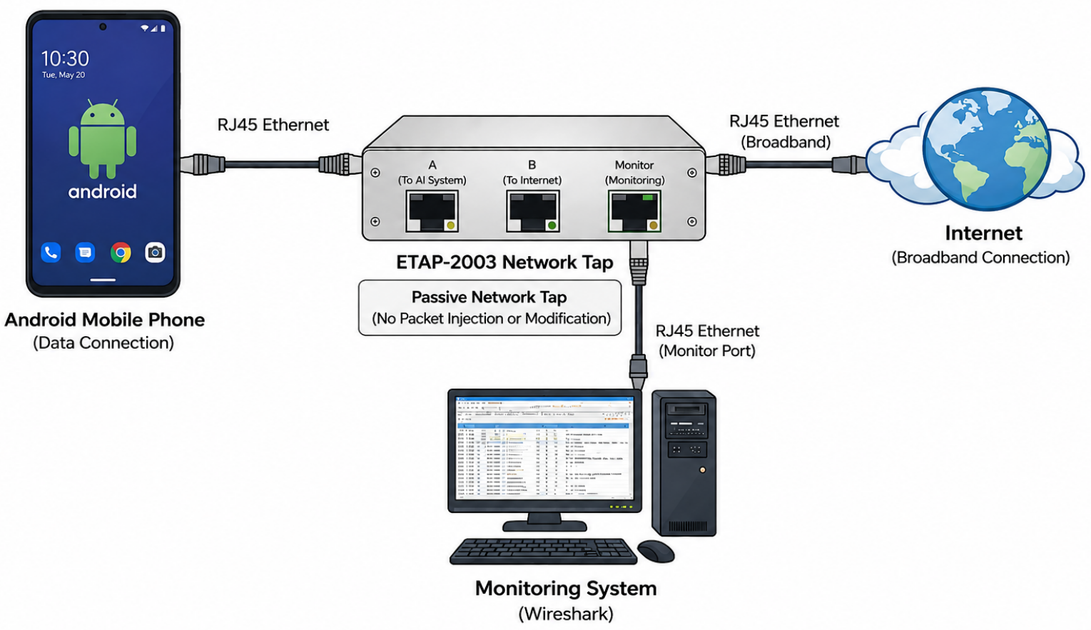
Figure 2.
Mean classification accuracy on the temporally held-out Day 5 test set for the single-flow baseline () and the validation-selected multi-flow configuration (). Results are averaged across five random seeds.
Figure 2.
Mean classification accuracy on the temporally held-out Day 5 test set for the single-flow baseline () and the validation-selected multi-flow configuration (). Results are averaged across five random seeds.
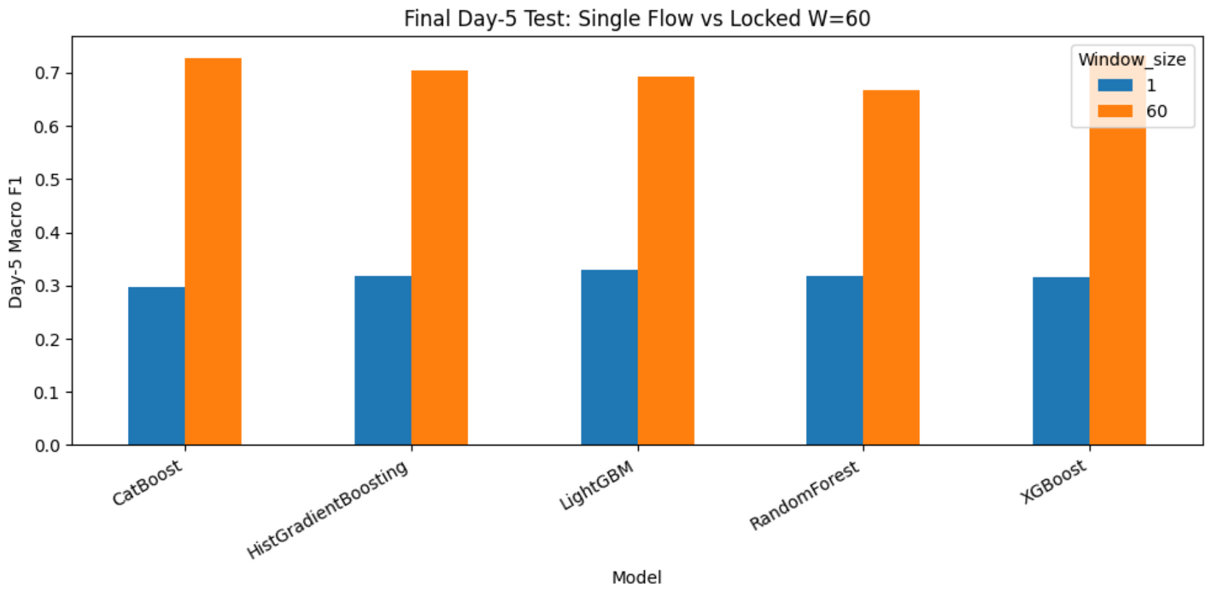
Figure 3.
Mean Macro F1-score on the temporally held-out Day 5 test set for the single-flow baseline () and the validation-selected multi-flow configuration (). Results are averaged across five random seeds.
Figure 3.
Mean Macro F1-score on the temporally held-out Day 5 test set for the single-flow baseline () and the validation-selected multi-flow configuration (). Results are averaged across five random seeds.
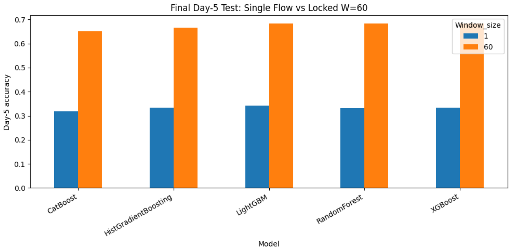
Figure 4.
Mean class-normalized confusion matrices for XGBoost on the temporally held-out Day 5 test set: (a) single-flow classification () and (b) the validation-selected multi-flow configuration ().
Figure 4.
Mean class-normalized confusion matrices for XGBoost on the temporally held-out Day 5 test set: (a) single-flow classification () and (b) the validation-selected multi-flow configuration ().
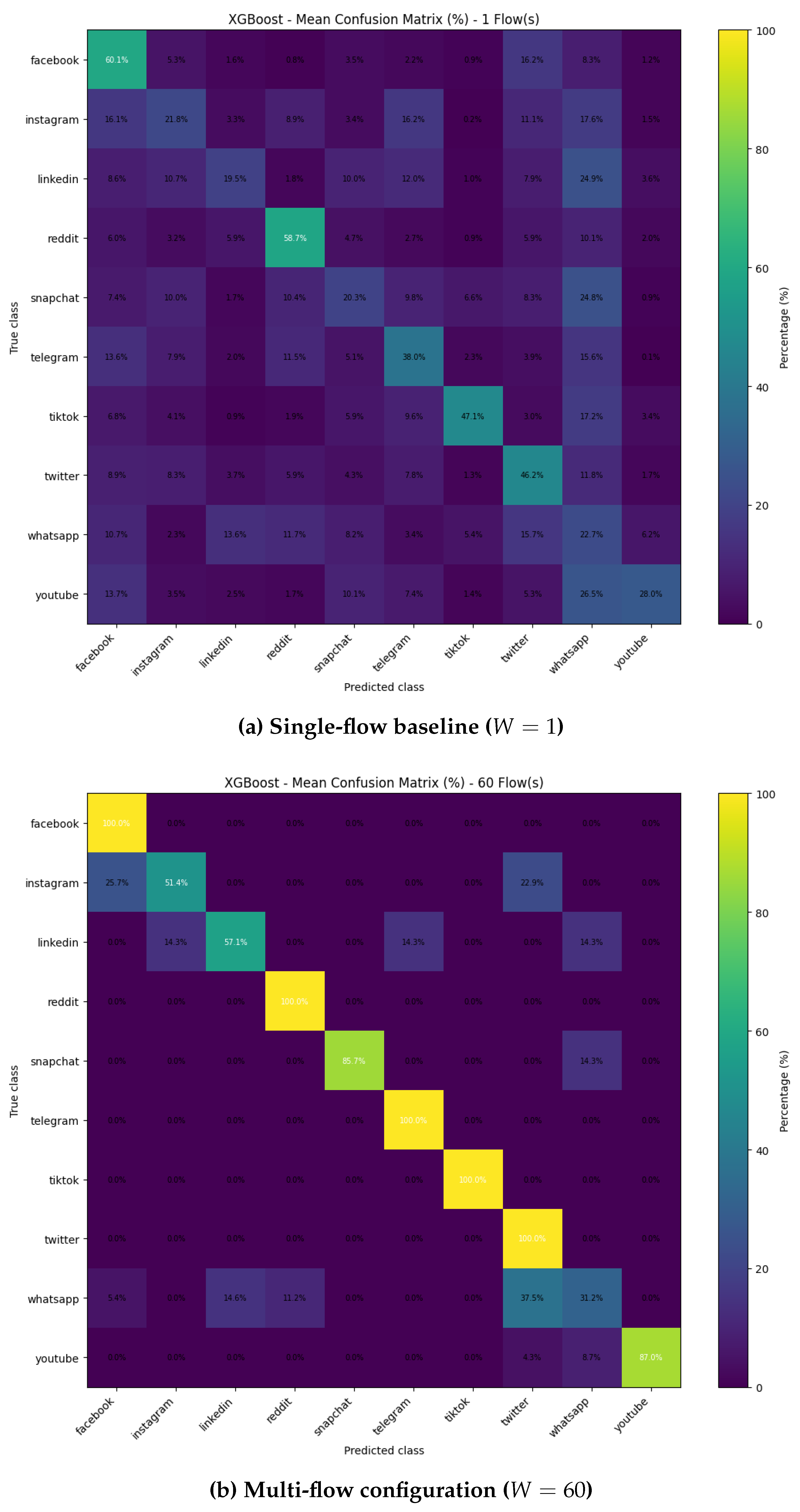
Figure 5.
Exact and semantic Jaccard agreement between the top-15 SHAP and LIME feature sets for the selected XGBoost model on the temporally held-out Day 5 test set.
Figure 5.
Exact and semantic Jaccard agreement between the top-15 SHAP and LIME feature sets for the selected XGBoost model on the temporally held-out Day 5 test set.
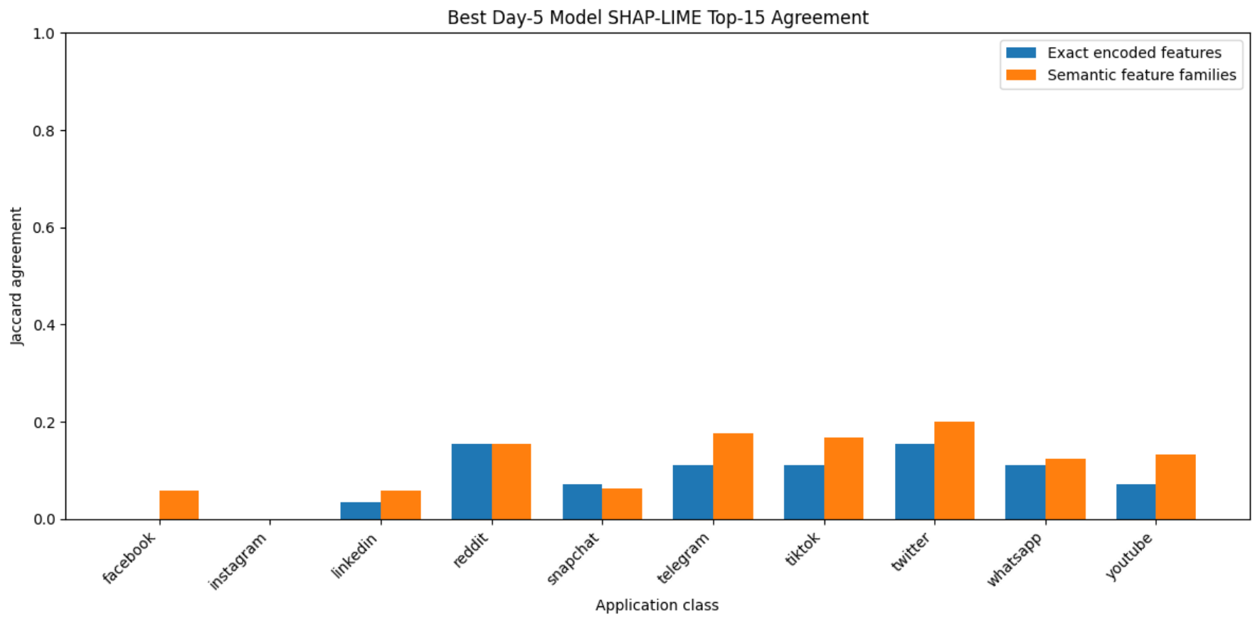
Table 1.
Final merged dataset distribution by application.
| Application | Capture Files | Flow Records | Percentage (%) |
|---|---|---|---|
| 5 | 3,225 | 12.84 | |
| 5 | 1,785 | 7.11 | |
| 5 | 1,576 | 6.27 | |
| 5 | 2,504 | 9.97 | |
| Snapchat | 5 | 2,113 | 8.41 |
| Telegram | 5 | 1,402 | 5.58 |
| TikTok | 5 | 1,607 | 6.40 |
| 5 | 3,040 | 12.10 | |
| 5 | 5,311 | 21.15 | |
| YouTube | 5 | 2,553 | 10.16 |
| Total | 50 | 25,116 | 100.00 |
Table 2.
Feature categories excluded before model training.
| Removal Category | Subcategory | Removed Features |
|---|---|---|
| Target and metadata | Target/capture information | Label, capture_day, capture_file |
| Flow identifiers | NFStream identifiers | id, expiration_id |
| Application leakage | NFStream application outputs | application_name, application_category_name, application_is_guessed, application_confidence |
| Application leakage | Server-name information | requested_server_name |
| Endpoint identifiers | Source endpoint | src_ip, src_mac, src_oui, src_port |
| Endpoint identifiers | Destination endpoint | dst_ip, dst_mac, dst_oui, dst_port |
| Raw sequence fields | SPLT representation | splt_direction, splt_ps, splt_piat_ms |
| Capture-time leakage | Absolute timestamps | All features ending in _first_seen_ms or _last_seen_ms |
Table 3.
Training hyperparameters for the benchmark models.
| Model | Hyperparameters |
|---|---|
| XGBoost | 800 estimators; learning rate = 0.04; maximum depth = 6; minimum child weight = 2; gamma = 0.02; subsample = 0.85; column sample = 0.85; L1 regularization = 0.05; L2 regularization = 1.5; histogram tree construction. |
| LightGBM | 800 estimators; learning rate = 0.04; 31 leaves; maximum depth = 8; minimum child size = 20; subsample = 0.85; feature sample = 0.85; L1 regularization = 0.05; L2 regularization = 1.5; balanced class weighting; early stopping = 40 rounds. |
| HistGradientBoosting | 700 maximum boosting iterations; learning rate = 0.05; maximum leaf nodes = 31; maximum depth = 8; minimum leaf size = 20; L2 regularization = 1.0; validation fraction = 0.15; early stopping after 30 iterations without improvement. |
| CatBoost | 800 iterations; learning rate = 0.05; tree depth = 7; L2 leaf regularization = 3.0; random strength = 0.5; early stopping = 40 rounds. |
| Random Forest | 600 trees; maximum depth = 15; minimum split size = 8; minimum leaf size = 3; square-root feature sampling; balanced-subsample class weighting. |
Table 4.
Validation performance across the five benchmark models and candidate multi-flow window sizes. Accuracy represents the five-seed mean, and Macro F1 is reported as mean ± standard deviation.
Table 4.
Validation performance across the five benchmark models and candidate multi-flow window sizes. Accuracy represents the five-seed mean, and Macro F1 is reported as mean ± standard deviation.
| Model | Window | Mean Accuracy | Mean Macro F1 & std | Complete Windows |
|---|---|---|---|---|
| CatBoost | 1 | 0.3931 | 0.3635 ± 0.0037 | 2491 |
| HistGradientBoosting | 1 | 0.3967 | 0.3733 ± 0.0121 | 2491 |
| LightGBM | 1 | 0.3640 | 0.3646 ± 0.0032 | 2491 |
| Random Forest | 1 | 0.3666 | 0.3733 ± 0.0023 | 2491 |
| XGBoost | 1 | 0.4045 | 0.3841 ± 0.0024 | 2491 |
| CatBoost | 20 | 0.7796 | 0.7392 ± 0.0107 | 108 |
| HistGradientBoosting | 20 | 0.8074 | 0.7824 ± 0.0092 | 108 |
| LightGBM | 20 | 0.8444 | 0.8272 ± 0.0065 | 108 |
| Random Forest | 20 | 0.8389 | 0.8359 ± 0.0037 | 108 |
| XGBoost | 20 | 0.8185 | 0.7959 ± 0.0155 | 108 |
| CatBoost | 40 | 0.7756 | 0.7404 ± 0.0155 | 41 |
| HistGradientBoosting | 40 | 0.8195 | 0.7872 ± 0.0286 | 41 |
| LightGBM | 40 | 0.9073 | 0.8960 ± 0.0149 | 41 |
| Random Forest | 40 | 0.9268 | 0.9227 ± 0.0000 | 41 |
| XGBoost | 40 | 0.8439 | 0.8128 ± 0.0177 | 41 |
| CatBoost | 60 | 0.9130 | 0.9133 ± 0.0000 | 23 |
| HistGradientBoosting | 60 | 0.9130 | 0.9056 ± 0.0000 | 23 |
| LightGBM | 60 | 0.9565 | 0.9467 ± 0.0000 | 23 |
| Random Forest | 60 | 0.9565 | 0.9467 ± 0.0000 | 23 |
| XGBoost | 60 | 0.9130 | 0.9056 ± 0.0000 | 23 |
| CatBoost | 80 | 0.8714 | 0.5905 ± 0.0346 | 14 |
| HistGradientBoosting | 80 | 0.9286 | 0.6524 ± 0.0000 | 14 |
| LightGBM | 80 | 0.9286 | 0.6333 ± 0.0000 | 14 |
| Random Forest | 80 | 0.9286 | 0.6333 ± 0.0000 | 14 |
| XGBoost | 80 | 0.9286 | 0.6524 ± 0.0000 | 14 |
Table 5.
Common validation score used for multi-flow window selection.
| Window | Common Macro F1 | Common Accuracy |
|---|---|---|
| 1 | 0.3718 | 0.3850 |
| 20 | 0.7961 | 0.8178 |
| 40 | 0.8318 | 0.8546 |
| 60 | 0.9236 | 0.9304 |
| 80 | 0.6324 | 0.9171 |
Table 6.
Top 15 SHAP features for the XGBoost classifier on correctly classified flows from the held-out Day 5 test set.
Table 6.
Top 15 SHAP features for the XGBoost classifier on correctly classified flows from the held-out Day 5 test set.
| Application | Top Feature | Mean | Application | Top Feature | Mean |
|---|---|---|---|---|---|
| dst2src_packets | 0.332788 | Telegram | dst2src_syn_packets | 1.102139 | |
| bidirectional_mean_ps | 0.257202 | bidirectional_max_ps | 0.475289 | ||
| src2dst_max_ps | 0.248232 | client_fingerprint_t13d1516h2_8daaf6152771_d8a... | 0.387200 | ||
| dst2src_bytes | 0.243204 | bidirectional_syn_packets | 0.331693 | ||
| dst2src_min_ps | 0.220080 | dst2src_max_piat_ms | 0.296086 | ||
| dst2src_mean_ps | 0.203915 | src2dst_max_ps | 0.274794 | ||
| dst2src_max_ps | 0.154075 | dst2src_min_piat_ms | 0.263017 | ||
| bidirectional_max_ps | 0.146577 | protocol | 0.209816 | ||
| src2dst_min_ps | 0.135257 | bidirectional_ack_packets | 0.209087 | ||
| bidirectional_stddev_ps | 0.111192 | bidirectional_mean_ps | 0.186410 | ||
| client_fingerprint_q00d0111h5_0f2cb44170f4_5e5... | 0.101885 | dst2src_stddev_piat_ms | 0.179969 | ||
| dst2src_duration_ms | 0.091102 | src2dst_bytes | 0.171696 | ||
| bidirectional_bytes | 0.074864 | dst2src_packets | 0.137441 | ||
| src2dst_mean_ps | 0.066910 | src2dst_max_piat_ms | 0.128980 | ||
| bidirectional_max_piat_ms | 0.063117 | src2dst_ack_packets | 0.125145 | ||
| bidirectional_min_ps | 0.297095 | TikTok | client_fingerprint_t13d181100_e8a523a41297_ef7... | 0.640973 | |
| dst2src_duration_ms | 0.231945 | dst2src_min_ps | 0.598016 | ||
| bidirectional_max_piat_ms | 0.223857 | server_fingerprint_2253c82f03b621c5144709b393f... | 0.502868 | ||
| src2dst_stddev_piat_ms | 0.177549 | client_fingerprint_t13d1516h2_8daaf6152771_e56... | 0.370536 | ||
| src2dst_stddev_ps | 0.136783 | server_fingerprint_15af977ce25de452b96affa2add... | 0.326676 | ||
| bidirectional_max_ps | 0.132960 | bidirectional_stddev_ps | 0.290641 | ||
| bidirectional_stddev_ps | 0.132126 | client_fingerprint_q13d0310h3_55b375c5d22e_cd8... | 0.222486 | ||
| src2dst_bytes | 0.125546 | src2dst_max_ps | 0.214036 | ||
| dst2src_min_ps | 0.123428 | dst2src_bytes | 0.190761 | ||
| src2dst_duration_ms | 0.122122 | bidirectional_max_ps | 0.187184 | ||
| bidirectional_stddev_piat_ms | 0.088483 | dst2src_max_ps | 0.150175 | ||
| bidirectional_mean_ps | 0.088339 | src2dst_bytes | 0.143890 | ||
| bidirectional_duration_ms | 0.088144 | bidirectional_min_ps | 0.126879 | ||
| src2dst_max_ps | 0.085376 | src2dst_psh_packets | 0.121060 | ||
| src2dst_max_piat_ms | 0.083985 | bidirectional_mean_ps | 0.091112 | ||
| dst2src_max_ps | 0.508430 | protocol | 0.699728 | ||
| dst2src_min_ps | 0.407092 | client_fingerprint_t13d0914h1_f91f431d341e_fad... | 0.355353 | ||
| src2dst_min_ps | 0.326838 | dst2src_min_ps | 0.163260 | ||
| bidirectional_max_ps | 0.202061 | bidirectional_max_ps | 0.157971 | ||
| src2dst_mean_ps | 0.172195 | src2dst_bytes | 0.140685 | ||
| bidirectional_min_ps | 0.165381 | bidirectional_stddev_ps | 0.139147 | ||
| bidirectional_mean_ps | 0.146888 | bidirectional_bytes | 0.138185 | ||
| dst2src_bytes | 0.145808 | server_fingerprint_eb1d94daa7e0344597e756a1fb6... | 0.134121 | ||
| src2dst_max_ps | 0.137347 | server_fingerprint_2b0648ab686ee45e0e7c35fcfb0... | 0.131962 | ||
| src2dst_bytes | 0.135923 | bidirectional_mean_ps | 0.119361 | ||
| bidirectional_stddev_ps | 0.131790 | src2dst_max_piat_ms | 0.111538 | ||
| bidirectional_stddev_piat_ms | 0.126266 | bidirectional_duration_ms | 0.107742 | ||
| src2dst_ack_packets | 0.108675 | dst2src_mean_ps | 0.093681 | ||
| bidirectional_max_piat_ms | 0.097927 | src2dst_max_ps | 0.091883 | ||
| dst2src_stddev_ps | 0.096918 | dst2src_bytes | 0.087545 | ||
| client_fingerprint_t12d1210h2_d34a8e72043a_f88... | 1.120868 | client_fingerprint_t13d1714h1_5b57614c22b0_fad... | 1.506852 | ||
| server_fingerprint_5b94af9bf6efc9dea4168416020... | 0.704908 | src2dst_psh_packets | 0.821396 | ||
| bidirectional_stddev_ps | 0.628397 | dst2src_mean_ps | 0.229200 | ||
| src2dst_bytes | 0.439952 | bidirectional_rst_packets | 0.209427 | ||
| client_fingerprint_t12d1209h2_d34a8e72043a_b39... | 0.266712 | bidirectional_max_ps | 0.179161 | ||
| bidirectional_bytes | 0.199799 | src2dst_min_ps | 0.170022 | ||
| bidirectional_max_ps | 0.147753 | dst2src_min_ps | 0.150682 | ||
| dst2src_mean_ps | 0.136463 | dst2src_max_ps | 0.148651 | ||
| bidirectional_min_ps | 0.130198 | dst2src_stddev_ps | 0.139165 | ||
| src2dst_max_ps | 0.118359 | dst2src_ack_packets | 0.133691 | ||
| dst2src_min_ps | 0.101753 | bidirectional_min_piat_ms | 0.123410 | ||
| bidirectional_duration_ms | 0.081198 | bidirectional_min_ps | 0.121172 | ||
| bidirectional_max_piat_ms | 0.070889 | dst2src_bytes | 0.117698 | ||
| server_fingerprint_a885fb01204bc11cc58efc02fe6... | 0.068242 | src2dst_max_ps | 0.103482 | ||
| dst2src_stddev_ps | 0.067454 | client_fingerprint_t00d0110h1_0f2cb44170f4_89a... | 0.092839 | ||
| Snapchat | client_fingerprint_t13d1516h2_8daaf6152771_e56... | 0.811171 | YouTube | src2dst_bytes | 0.409261 |
| client_fingerprint_q13d0310h3_55b375c5d22e_cd8... | 0.531051 | dst2src_min_ps | 0.377655 | ||
| bidirectional_stddev_ps | 0.204338 | client_fingerprint_q13d0311h3_55b375c5d22e_653... | 0.319356 | ||
| dst2src_max_ps | 0.197126 | bidirectional_min_ps | 0.277875 | ||
| src2dst_bytes | 0.170572 | dst2src_max_piat_ms | 0.248822 | ||
| dst2src_mean_ps | 0.169681 | server_fingerprint_eb1d94daa7e0344597e756a1fb6... | 0.210549 | ||
| bidirectional_max_ps | 0.161496 | src2dst_min_ps | 0.202489 | ||
| dst2src_min_ps | 0.144493 | dst2src_duration_ms | 0.179228 | ||
| src2dst_max_ps | 0.134064 | bidirectional_stddev_ps | 0.170843 | ||
| bidirectional_bytes | 0.125730 | dst2src_bytes | 0.147797 | ||
| src2dst_mean_ps | 0.120081 | dst2src_max_ps | 0.145723 | ||
| bidirectional_mean_ps | 0.108893 | src2dst_mean_ps | 0.129398 | ||
| src2dst_psh_packets | 0.108299 | bidirectional_duration_ms | 0.124648 | ||
| bidirectional_syn_packets | 0.107317 | bidirectional_max_ps | 0.120866 | ||
| dst2src_duration_ms | 0.102874 | bidirectional_bytes | 0.112933 |
Table 7.
Top 15 LIME features for each application class using the selected XGBoost model.
| Application | Top Features | Mean | Application | Top Features | Mean |
|---|---|---|---|---|---|
| client_fingerprint_q00d0109h5_0f2cb44170f4_5d0... | 0.168849 | Telegram | client_fingerprint_t12d1210h2_d34a8e72043a_f88... | 0.032225 | |
| dst2src_min_piat_ms | 0.147371 | client_fingerprint_t13d181100_e8a523a41297_ef7... | 0.022742 | ||
| client_fingerprint_t12d1210h2_d34a8e72043a_f88... | 0.118280 | client_fingerprint_t13d1516h2_8daaf6152771_d8a... | 0.022302 | ||
| client_fingerprint_q13d0208h2_ec078ce24869_51c... | 0.115654 | src2dst_duration_ms | 0.017847 | ||
| client_fingerprint_t00d0309h2_55b375c5d22e_381... | 0.099760 | client_fingerprint_t13d1516h2_8daaf6152771_027... | 0.010928 | ||
| client_fingerprint_t13d181100_e8a523a41297_ef7... | 0.092860 | server_fingerprint_2253c82f03b621c5144709b393f... | 0.009711 | ||
| server_fingerprint_eb1d94daa7e0344597e756a1fb6... | 0.068048 | dst2src_min_piat_ms | 0.009379 | ||
| server_fingerprint_2253c82f03b621c5144709b393f... | 0.060054 | client_fingerprint_1,3,6,15,26,28,51,58,59,43 | 0.009238 | ||
| client_fingerprint_q13d0310h3_55b375c5d22e_cd8... | 0.045610 | client_fingerprint_t00d0108h1_0f2cb44170f4_8e1... | 0.008960 | ||
| client_fingerprint_t13d1516h2_8daaf6152771_027... | 0.044891 | client_fingerprint_t13d0108h2_0f2cb44170f4_52e... | 0.008617 | ||
| server_fingerprint_d7e12962b60127bdbe4f65f3922... | 0.037934 | client_fingerprint_q13d0310h3_55b375c5d22e_cd8... | 0.008587 | ||
| client_fingerprint_t13d1516h2_8daaf6152771_e56... | 0.033423 | src2dst_bytes | 0.008485 | ||
| server_fingerprint_a5b7547fb0048cdf45300719110... | 0.026977 | client_fingerprint_t13d0914h1_f91f431d341e_fad... | 0.008468 | ||
| server_fingerprint_5badad76fbdd6e8b6296e2e9f40... | 0.023338 | server_fingerprint_df91478bfbf2ad437dd1c8b73a4... | 0.008178 | ||
| client_fingerprint_t13d1712h2_5b57614c22b0_3f5... | 0.013736 | client_fingerprint_t12d1209h1_d34a8e72043a_b39... | 0.007217 | ||
| client_fingerprint_t13d0207h2_ec078ce24869_e91... | 0.051364 | TikTok | client_fingerprint_t13d181100_e8a523a41297_ef7... | 0.606476 | |
| client_fingerprint_t12d1210h2_d34a8e72043a_f88... | 0.040967 | server_fingerprint_2253c82f03b621c5144709b393f... | 0.392672 | ||
| ip_version | 0.034734 | server_fingerprint_15af977ce25de452b96affa2add... | 0.080788 | ||
| client_fingerprint_t13d181100_e8a523a41297_ef7... | 0.031938 | client_fingerprint___RARE__ | 0.069277 | ||
| server_fingerprint_a5b7547fb0048cdf45300719110... | 0.018251 | client_fingerprint_t12d1210h2_d34a8e72043a_f88... | 0.049423 | ||
| server_fingerprint_2253c82f03b621c5144709b393f... | 0.017194 | server_fingerprint_df91478bfbf2ad437dd1c8b73a4... | 0.031012 | ||
| client_fingerprint_t13d1516h2_8daaf6152771_027... | 0.015719 | client_fingerprint_t12d1209h1_d34a8e72043a_b39... | 0.030240 | ||
| client_fingerprint_q13d0310h3_55b375c5d22e_cd8... | 0.015412 | server_fingerprint_20276646585c81d93770671389c... | 0.023218 | ||
| server_fingerprint_d7e12962b60127bdbe4f65f3922... | 0.015110 | client_fingerprint_t13d181100_e8a523a41297_d5f... | 0.017779 | ||
| client_fingerprint_t13d1516h2_8daaf6152771_e56... | 0.014484 | client_fingerprint_t12d1410h1_c866b44c5a26_f88... | 0.017709 | ||
| dst2src_min_piat_ms | 0.010779 | client_fingerprint_1,3,6,15,31,33,43,44,46,47,... | 0.014681 | ||
| client_fingerprint_t13d0914h1_f91f431d341e_fad... | 0.009374 | server_fingerprint_a7ee24108d2f6fe0b6b629f4b4f... | 0.014642 | ||
| client_fingerprint_t00d0108h1_0f2cb44170f4_8e1... | 0.009368 | server_fingerprint_bfc90d56141386ee83b56cda231... | 0.013483 | ||
| client_fingerprint_t13i1713h1_5b57614c22b0_fad... | 0.009174 | client_fingerprint_t13d1516h2_8daaf6152771_027... | 0.013031 | ||
| client_fingerprint_t00d0310h2_55b375c5d22e_50c... | 0.008145 | client_fingerprint_t13d0207h2_ec078ce24869_e91... | 0.012671 | ||
| client_fingerprint_t13d1516h2_8daaf6152771_027... | 0.334333 | client_fingerprint_t13d0914h1_f91f431d341e_fad... | 0.329914 | ||
| client_fingerprint_t12d1210h2_d34a8e72043a_f88... | 0.084051 | client_fingerprint_t13d0913h2_f91f431d341e_eca... | 0.158114 | ||
| client_fingerprint_t13d181100_e8a523a41297_ef7... | 0.066321 | server_fingerprint_eb1d94daa7e0344597e756a1fb6... | 0.085786 | ||
| server_fingerprint_2253c82f03b621c5144709b393f... | 0.038593 | protocol | 0.059954 | ||
| client_fingerprint_q13d0310h3_55b375c5d22e_cd8... | 0.035827 | client_fingerprint_t12d1210h2_d34a8e72043a_f88... | 0.058900 | ||
| client_fingerprint_t13d1516h2_8daaf6152771_e56... | 0.035657 | client_fingerprint_t13d1713h1_5b57614c22b0_eca... | 0.058112 | ||
| src2dst_min_ps | 0.032637 | server_fingerprint_2b0648ab686ee45e0e7c35fcfb0... | 0.047811 | ||
| server_fingerprint_9d9ce860f1b1cbef07b019450cb... | 0.030002 | ip_version | 0.045027 | ||
| server_fingerprint___RARE__ | 0.028443 | client_fingerprint_t13d181100_e8a523a41297_ef7... | 0.040836 | ||
| client_fingerprint_1,3,6,15,44,33 | 0.020656 | client_fingerprint_q13d0108h2_0f2cb44170f4_ffa... | 0.038273 | ||
| client_fingerprint_1,3,6,15,26,28,51,58,59,43 | 0.020093 | client_fingerprint_q13d0210h2_ec078ce24869_89a... | 0.030835 | ||
| server_fingerprint_bfc90d56141386ee83b56cda231... | 0.018245 | server_fingerprint_2253c82f03b621c5144709b393f... | 0.029627 | ||
| client_fingerprint_t13i1713h1_5b57614c22b0_fad... | 0.017796 | client_fingerprint_t13d1516h2_8daaf6152771_027... | 0.024449 | ||
| client_fingerprint_t13d0912h2_f91f431d341e_402... | 0.017599 | client_fingerprint_t13d0912h2_f91f431d341e_402... | 0.015483 | ||
| client_fingerprint_t13d0108h2_0f2cb44170f4_52e... | 0.016253 | client_fingerprint_q13d0310h3_55b375c5d22e_cd8... | 0.014435 | ||
| client_fingerprint_t12d1210h2_d34a8e72043a_f88... | 0.777301 | client_fingerprint_t12d1210h2_d34a8e72043a_f88... | 0.246219 | ||
| server_fingerprint_5b94af9bf6efc9dea4168416020... | 0.158438 | client_fingerprint_t13d1714h1_5b57614c22b0_fad... | 0.222126 | ||
| client_fingerprint_t12d1209h2_d34a8e72043a_b39... | 0.113922 | client_fingerprint_t13d181100_e8a523a41297_ef7... | 0.190948 | ||
| server_fingerprint_a885fb01204bc11cc58efc02fe6... | 0.107896 | dst2src_min_piat_ms | 0.182043 | ||
| client_fingerprint_t13d1615h2_46e7e9700bed_45f... | 0.100076 | server_fingerprint_2253c82f03b621c5144709b393f... | 0.108800 | ||
| client_fingerprint_t13d181100_e8a523a41297_ef7... | 0.048366 | client_fingerprint_q13d0108h2_0f2cb44170f4_ffa... | 0.093506 | ||
| server_fingerprint_20276646585c81d93770671389c... | 0.031180 | bidirectional_min_piat_ms | 0.092609 | ||
| server_fingerprint_9ebc57def2efb523f25c77af13a... | 0.023670 | client_fingerprint_q13d0310h3_55b375c5d22e_cd8... | 0.090317 | ||
| server_fingerprint_2253c82f03b621c5144709b393f... | 0.022244 | client_fingerprint_t13d1516h2_8daaf6152771_027... | 0.086123 | ||
| client_fingerprint_q13d0310h3_55b375c5d22e_cd8... | 0.018919 | client_fingerprint_t00d0110h1_0f2cb44170f4_89a... | 0.064813 | ||
| client_fingerprint_t13d1516h2_8daaf6152771_027... | 0.018073 | client_fingerprint_t13d1516h2_8daaf6152771_e56... | 0.061346 | ||
| server_fingerprint_5badad76fbdd6e8b6296e2e9f40... | 0.016565 | client_fingerprint_t13d0108h2_0f2cb44170f4_52e... | 0.057929 | ||
| client_fingerprint_1,3,6,15,26,28,51,58,59,43 | 0.014592 | server_fingerprint_df91478bfbf2ad437dd1c8b73a4... | 0.050699 | ||
| server_fingerprint_df91478bfbf2ad437dd1c8b73a4... | 0.012006 | client_fingerprint_t00d0108h1_0f2cb44170f4_8e1... | 0.045335 | ||
| client_fingerprint_q13d0208h2_ec078ce24869_51c... | 0.010838 | client_fingerprint_1,3,6,15,26,28,51,58,59,43 | 0.043047 | ||
| Snapchat | client_fingerprint_q13d0310h3_55b375c5d22e_cd8... | 0.335543 | YouTube | server_fingerprint_eb1d94daa7e0344597e756a1fb6... | 0.053792 |
| client_fingerprint_t13d1516h2_8daaf6152771_e56... | 0.331568 | client_fingerprint_t12d1210h2_d34a8e72043a_f88... | 0.047777 | ||
| client_fingerprint_t12d1210h2_d34a8e72043a_f88... | 0.093362 | client_fingerprint_t13d181100_e8a523a41297_ef7... | 0.037316 | ||
| client_fingerprint_t13d181100_e8a523a41297_ef7... | 0.073873 | client_fingerprint_q13d0311h3_55b375c5d22e_653... | 0.034890 | ||
| server_fingerprint_2253c82f03b621c5144709b393f... | 0.039369 | client_fingerprint_t13d1516h2_8daaf6152771_027... | 0.021359 | ||
| client_fingerprint_t13d1516h2_8daaf6152771_027... | 0.033943 | server_fingerprint_2253c82f03b621c5144709b393f... | 0.020639 | ||
| client_fingerprint_t13d0914h1_f91f431d341e_fad... | 0.024819 | client_fingerprint_q13d0310h3_55b375c5d22e_cd8... | 0.019972 | ||
| client_fingerprint_1,3,6,15,44,33 | 0.022044 | client_fingerprint_t00d0108h1_0f2cb44170f4_8e1... | 0.018512 | ||
| client_fingerprint_t00d0108h1_0f2cb44170f4_8e1... | 0.021248 | client_fingerprint_q13d0313h3_55b375c5d22e_226... | 0.015761 | ||
| server_fingerprint_20276646585c81d93770671389c... | 0.020632 | client_fingerprint_t13d1516h2_8daaf6152771_e56... | 0.014559 | ||
| server_fingerprint_df91478bfbf2ad437dd1c8b73a4... | 0.020395 | server_fingerprint_9d9ce860f1b1cbef07b019450cb... | 0.012546 | ||
| client_fingerprint_t13d1714h1_5b57614c22b0_fad... | 0.020378 | client_fingerprint_1,3,6,15,31,33,43,44,46,47,... | 0.011529 | ||
| bidirectional_duration_ms | 0.016442 | client_fingerprint_t13d0912h2_f91f431d341e_402... | 0.011242 | ||
| client_fingerprint_1,3,6,15,31,33,43,44,46,47,... | 0.014576 | client_fingerprint_t13d181100_e8a523a41297_d5f... | 0.010475 | ||
| client_fingerprint_t13i1713h1_5b57614c22b0_fad... | 0.013759 | server_fingerprint_0b0a9cfc3785af170571d2e1996... | 0.009017 |
Disclaimer/Publisher’s Note: The statements, opinions and data contained in all publications are solely those of the individual author(s) and contributor(s) and not of MDPI and/or the editor(s). MDPI and/or the editor(s) disclaim responsibility for any injury to people or property resulting from any ideas, methods, instructions or products referred to in the content. |
© 2026 by the authors. Licensee MDPI, Basel, Switzerland. This article is an open access article distributed under the terms and conditions of the Creative Commons Attribution (CC BY) license (http://creativecommons.org/licenses/by/4.0/).
Copyright: This open access article is published under a Creative Commons CC BY 4.0 license, which permit the free download, distribution, and reuse, provided that the author and preprint are cited in any reuse.