

Submitted:
02 September 2026
Posted:
03 September 2026
You are already at the latest version
Abstract
This study considers the simulation of hydrological processes in the Mzymta River (Russian Federation) using the Regularized Physics-Informed Neural Networks (PINNs).
The Mzymta is the longest river in the Russian Federation that flows into the Black Sea.
To formulate the boundary value problem, data on river topography (bottom profile) and hydrological measurements (time series of water level and discharge) from the gauging stations near the settlements of Rosa Khutor, Gorki-Gorod, Krasnaya Polyana, and Kazachiy Brod were collected.
This study considers two modeling scales: the full-scale problem and a local-scale formulation for a short river segment, characterized by bed slope flattening, the development of a backwater--drawdown profile, and the occurrence of a hydraulic jump.
The Saint-Venant system of equations was considered as a mathematical model.
To solve this problem, we implemented PINNs.
Two problem statements were considered: stationary and non-stationary.
The full-scale simulation revealed that at the entire river scale, the flow rapidly establishes a normal depth profile, with all local perturbations being smoothed out by friction and thus indistinguishable at this resolution. In the unsteady case, the flow profile undergoes perturbations that propagate downstream in response to the time-varying sinusoidal inlet discharge. These perturbations propagate downstream at a finite speed, which is determined by the characteristic velocities of the shallow-water system.
The local-scale formulation allowed us to capture the deviation of the flow profile from the normal depth and to study the backwater--drawdown problem, which involves the formation of a hydraulic jump both in stationary and non-stationary formulations.
The formation of a hydraulic jump required the introduction of regularization into the loss function, since in the vicinity of the jump, the solution ceases to be smooth and experiences a discontinuity. To capture the discontinuity, we applied a method of relaxing the momentum equation term near the jump region. To enhance the sharpness of the jump, we additionally introduced a term that minimizes the width of the jump region.
To properly account for all terms in the loss function, adaptive weighting of the coefficients was employed.
Verification of the PINNs was performed by comparing the results against the fourth-order Runge–Kutta method, for both smooth solutions and those involving a hydraulic jump.
Keywords:
Physics-Informed Neural Networks
; Saint-Venant shallow water equations
; loss function regularization
; hydraulic jump
1. Introduction
Climate change is currently exerting a significant influence on water resources management. Specifically, alterations in the hydrological cycle complicate management practices, while the increasing frequency and intensity of extreme events place considerable strain on hydraulic structures and associated infrastructure [1].
Climate change is transforming water resources management from a routine task into a domain of continuous risk analysis and strategic planning. The development of flexible and resilient strategies has become a key priority for ensuring water security [2].
Mathematically, the study of flood phenomena can be formulated as the solution of forward and inverse hydrological problems by applying equations derived from the theory of shallow water. Physics-Informed Neural Networks (PINNs) have been increasingly applied in digital twin frameworks that combine physical models with data-driven methods [3,4,5]. In these models, the residuals of the partial differential equations are directly embedded into the loss function of the neural network. PINNs have been used for both forward solution and inverse parameter-identification problems [6,7,8]. The modern theory of inverse problems for hyperbolic equations is presented in a number of works [9,10]. Early studies in the field of numerical methods for solving inverse hydrological problems [11,12] applied various mathematical approaches to solve the Saint-Venant equations [10,13,14].
Early studies focused on assessing the capabilities of PINNs for solving hydrological problems, particularly for approximating one-dimensional shallow water equations. In [15,16], PINNs were used to assimilate observational data while solving the one-dimensional Saint-Venant equations. The performance of PINNs was evaluated by comparing the results with analytical solutions and numerical simulation data.
Numerical solutions of the one-dimensional equations were used to predict water level profiles in rivers, as well as to estimate the so-called roughness parameter [17]. PINNs models were implemented within the TensorFlow machine learning library using two neural networks. Different activation functions, numbers of layers, and numbers of neurons in the hidden layers were tested.
The aim of the dissertation work [18] was to investigate the applicability of PINNs for approximating the shallow water equations (SWE), which represent a system of PDEs used for modeling free-surface flows and the two-dimensional dam-break problem.
PINNs have also been applied to flow and transport problems in porous media, including the Darcy and Richards equations. For instance, the PINNs method was introduced for solving a coupled system (the Darcy equation and the advection–dispersion equation) and was tested over a range of Péclet numbers. The authors of [19] incorporated finite volume method-based numerical solutions as a reference to evaluate the PINNs results when determining the steady-state hydraulic head and concentration in the coupled system characterized by spatially varying conductivity and velocity fields. The PINNs approach enables the generation of numerical data in real time, which can then be used for modeling riverbed siltation. The prediction of key indicators plays a crucial role in reducing river pollution caused by siltation.
In [20], the researchers conducted a comparative analysis of the PINNs approach and traditional numerical methods for estimating flow velocity, pressure and density in water systems. The PINNs architecture was applied to solve the partial differential equation describing water infiltration into soil, enabling a numerical analysis of the infiltration process. The modeling results for vertical infiltration in the water-soil system demonstrated high accuracy and lower error levels compared to classical methods. Among the studied soils, water infiltrated fastest in light soil, followed by heavy soil, with the lowest infiltration rate observed in medium soil [21]. Several key soil parameters are required to reproduce water processes in soils using the Richardson–Richards equation (RRE). These include water retention curves (WRC) and hydraulic conductivity functions (HCF). Commonly used methods for obtaining WRC and HCF are often inadequate for such modeling.
In [22,23], it was shown that the PINNs approach can overcome this limitation and yield an inverse solution for the RRE, enabling the estimation of WRC and HCF from volumetric water content measurements without requiring initial or boundary conditions.
In [24], PINNs were employed to solve the inverse problem of unsaturated groundwater flow by incorporating observed volumetric water content data directly into the network loss function. Specifically, the Richards equation was coupled with the van Genuchten constitutive model, and PINNs were trained to recover both the spatially distributed solutions of the Richards equation and the unknown parameters of the van Genuchten model from sparse measurement data.
Berardi et al. [25] extended this approach to an adaptive inverse PINNs architecture for various transport models in porous media, including diffusion, advection–diffusion–reaction systems, and mobile–immobile phase formulations. In their method, transport parameters such as diffusion coefficients were treated as trainable variables, and the loss function components (data mismatch, initial and boundary conditions and PDE residuals) were adaptively weighted during training to ensure robust convergence.
In [26], the authors enhanced the PINNs methodology by proposing gradient-enhanced PINNs (gPINNs), in which the loss function includes not only PDE residual terms but also gradient information. Numerical experiments demonstrated that gPINNs achieve higher accuracy and faster convergence compared to standard PINNs, while requiring fewer collocation points for both forward and inverse problems.
Finally, Difonzo et al. [27] applied PINNs to estimate the horizon parameter in peridynamic models of linear microelasticity. The authors investigated several kernel functions (hat, distributed, and V-shaped kernels) and conducted numerical experiments in one- and two-dimensional settings. By treating the horizon size as an additional trainable parameter, they demonstrated that PINNs can accurately recover the nonlocal interaction scale directly from simulated data.
A specific application of PINNs was proposed in [28] for solving the shallow water equations (SWE) on a sphere. The trained PINNs outperformed conventional numerical methods such as finite difference, finite volume, and spectral methods in solving the differential equations.
Recent approaches in the application of PINNs and hybrid neural network architectures for studying hydrological processes in rivers are presented in [29,30,31,32,33,34]. In recent studies, PINNs and other machine learning methods have been actively applied to model climate-driven processes described by partial differential equations. Such approaches combine physical constraints with data-driven learning [3,4,5,35,36]. The development of PINNs architectures in fluid dynamics has focused on evolutionary deep neural networks [37,38,39,40]. A review of modern approaches in the application of PINNs to fluid dynamics is given in [41,42,43,44,45,46]. The work [47] presents an overview of the application of PINNs and PIKANs in physics-informed machine learning. The authors of [48] explore the use of an energy transformer approach to reconstruct three different flow fields from sparse measurement data.
Currently, there exist other approaches to constructing PINNs architectures based on operator neural networks (DeepONet) [49] and Fourier neural operators (FNO) [50]. However, their software implementation is more complex.
For solving inverse problems using PINNs, a careful selection of optimizers is required to compute the gradient of the loss function and find the optimal parameters of the neural network. A review of various optimizers, including GradNorm, PCGrad, Multi-Objective Optimization, and Self-Adaptive PINNs, was conducted by Italian authors in [25]. They developed a novel Adaptive-Inverse PINNs method, in which the loss function weights are computed at each iteration, and applied it to solve a one-dimensional inverse transport problem in porous media.
In the last five years, graph neural networks have been actively developed for studying hydrological processes in rivers. Notable research groups in this area include the team from Delft University of Technology, Delft, the Netherlands, with the mSWE-GNN project; the group from Southern University of Science and Technology, Shenzhen, China, working on graph models (ChebNet, GAT, GraphSAGE, GCNII, GCN, and GIN) as well as Entity-Aware LSTM; the team from Utah State University, Logan, UT, USA, developing a spatio-temporal graph neural network (STGNN); the collaboration between the US Army Corps of Engineers Vicksburg District, Mississippi, USA and the University of New Orleans, Louisiana, USA, working on the PINN-HEC-RAS project; the group from the University of Virginia, Virginia, USA, in collaboration with Nvidia, developing HydroGraphNet, which employs a GNN-KAN model; and the team from Rice University, Houston, TX, USA, with the FloodGNN-GRU project.
The implementation of digital twins for rivers enables a proactive approach to water resources management, allowing problems to be anticipated and mitigated in near real-time. Furthermore, digital twins can provide forecasts under scenario-based changes that cannot be reproduced in field conditions. River digital twins are often built upon hydrological models for runoff generation (e.g., SWAT, HEC-HMS), as well as hydrodynamic models (e.g., Delft3D, HEC-RAS, TELEMAC, MIKE 21). At the same time, artificial intelligence methods are developing rapidly, including PINNs, Graph Neural Networks (GNN), transformers for time series, DeepONet, and Gaussian Processes for improving predictions and uncertainty quantification. High-performance computing is widely employed, including GPUs, distributed computing, and cloud platforms. Modern hybrid digital twins combine physics-based laws with machine learning techniques.
The study by [15] employed PINNs to downscale a large-scale river model to a subgrid resolution. The proposed PINNs framework successfully solved the unsteady one-dimensional Saint-Venant equations, incorporated periodic tidal boundary conditions via Fourier feature embeddings, assimilated heterogeneous data sources, and was coupled with a large-scale river model to produce downscaled solutions.
The study [51] introduced FNOCL, a deep learning neural network for modeling unsteady natural river flows. FNOCL is based on the FNO by incorporating Convolutional Long Short-Term Memory (ConvLSTM) layers, combining robust performance with high efficiency in capturing spatiotemporal patterns. It is claimed that the network effectively handles the complexities of spatial and temporal variations. FNOCL accounts for complex river cross-sectional profiles, enabling accurate flow dynamics modeling in complex river morphologies. In this study, FNOCL is applied to two distinct river networks with varying morphological complexity. Furthermore, FNOCL demonstrates a significant speedup compared to HEC-RAS, achieving, in particular, a 50-fold increase in a complex river network.
The study [52] investigates the potential of using the FNO as a physics-informed surrogate for one-dimensional debris flow modeling, applied to the Rendinara–Morino system in central Italy. To address the challenges of limited observational data and the computational cost of high-fidelity solvers, a validated finite-volume shallow-water model is combined with operator learning to create a site-specific digital twin of debris flow dynamics. Overall, the study demonstrates that integrating physics-based synthetic data with operator learning architectures provides a viable path for constructing accurate, computationally efficient, and site-specific approximations for debris flow modeling under data-scarce conditions.
In this study, we focus on modeling the flow of the Mzymta River in the vicinity of Sochi, Russia. The research is based on the authors’ previous work [53], which was devoted to the inverse problem for the determination of the Manning coefficient using PINNs. The Mzymta is a typical mountain river, characterized by steep slopes, rapidly varying discharges, wave-dominated processes, and complex geometry. For such rivers, classical 1D models often struggle with unknown roughness, incomplete data, and sparse measurements. PINNs can employ physics as a regularizer and extract information even from a limited number of observations.
The paper is organized as follows. Section 1 contains an introduction that provides a brief overview of the research area. Section 2 covers the mathematical model for hydrological problems: Saint-Venant shallow water equations (Section 2.1), initial and boundary conditions (Section 2.2), non-dimensionalization of the SWE equations (Section 2.3) and the stationary problems statement peculiarities (Section 2.4). Section 3 covers the method for solving the problem: Fully-Connected Neural Network (Section 3.1), Physics-Informed Neural Networks (Section 3.2), smart boundary conditions (Section 3.3), hydraulic jump regularization (Section 3.4), Balancing the weights of the loss function components (Section 3.5). Section 4 covers the description of the considered Mzymta River and the data for its simulation. Section 5 covers the main results: full scale flow of the Mzymta River, stationary (Section 5.1) and non-stationary (Section 5.2); short flattening reach with transition from supercritical to subcritical flow, stationary (Section 5.3) and non-stationary (Section 5.4). Section 6 covers the discussion, where both the results obtained and the hardware implementation are discussed. Section 7 provides the conclusions and outlines future research plans.
2. Mathematical Model
To model the flow of the Mzymta River, we employ a one-dimensional unsteady Saint-Venant model. One-dimensional models are applicable when the flow exhibits a dominant direction. The Mzymta River flows within a single main channel, which makes the 1D approach physically justified. The Saint-Venant Shallow Water Equations (SWE) assume hydrostatic pressure distribution, which is valid when vertical accelerations are negligible. This condition is satisfied when the bed slope is less than 10% and the flow scale is much larger than the river depth. The slope of the Mzymta River does not exceed this threshold at the full-river scale. 1D models require fewer computational resources and less input data than 2D models, making them suitable for rapid scenario assessment. The 1D model is optimal when the flow is primarily confined to the channel and there is no extensive floodplain inundation that would require a 2D approach – which is exactly the case considered in this study.
2.1. Saint-Venant Shallow Water Equations
Consider a one-dimensional problem of water flow in a channel of constant width W [m] and length L [m] (Figure 1). The coordinate along the channel is denoted as , and the time variable as t. The channel has a bottom elevation profile z [m] above sea level. At each point, the flow has a depth h [m] and a longitudinal cross-sectionally averaged velocity u [m/s]. The water discharge through a cross-section of the river is q [/s] . The flow is accelerated by gravity g [m/] and decelerated by bottom friction, characterized by the bottom roughness coefficient n [s/] according to the Manning formula [54].
The flow in the shallow channel is described by the Saint-Venant Shallow Water Equations. The continuity equation takes the following form:
and the momentum equation is written as follows
We assume that the bed slope is negative and the flow velocity u is positive, which reflects the physical condition that the flow is directed downstream and cannot go uphill.
2.2. Initial and Boundary Conditions
The system (1)-(2) is of mixed hyperbolic-parabolic type. To close it, initial and boundary conditions must be specified. We seek the solution in the domain . The initial conditions are written as:
Since the system consists of two first-order equations, two boundary conditions must be specified: one for the discharge and one for the depth. The location of each boundary condition (inlet or outlet) depends on the specific conditions of the characteristics at the boundaries of the domain. Since water always flows into the domain at the inlet boundary, the boundary condition for discharge is imposed at the inlet cross-section:
For the depth, the imposition of the boundary condition depends on the flow regime. In subcritical flow, the characteristics propagate upstream, and the depth is specified at the outlet. In supercritical flow, conversely, the characteristics propagate downstream, and the depth is specified at the inlet:
However, in the problem under consideration, mixed flow regimes may occur (subcritical in one region and supercritical in another). In this case, the boundary conditions become more complicated. For example, a situation may arise where the depth h is prescribed both at the inlet (supercritical regime) and at the outlet (subcritical regime). Alternatively, the depth may not be prescribed at either the inlet or the outlet boundaries (if the flow is subcritical at the inlet and supercritical at the outlet).
2.3. Non-Dimensionalization of the SWE
To solve the problem using PINNs, it is necessary to non-dimensionalize the equations and the boundary conditions. This is because neural networks can effectively capture the nonlinearity of the problem when the input data lie in the vicinity of unity, since it is precisely in this range that the activation function exhibits substantially nonlinear behavior.
For non-dimensionalization of the equations let us introduce the characteristic scale parameters: time T, length L, depth H, and velocity U. We write down the relations between the dimensional and dimensionless (denoted by the symbol ) variables as follows:
We decompose the bottom slope into the product of a characteristic slope Sl and a normalized slope . Note that and take negative values, while Sl and are positive.
We introduce the dimensionless complexes characterizing the system:
- The Strouhal number which characterizes the time scale of the problem and its unsteadiness;
- The Froude number , which characterizes the gravitational component of acceleration;
- The Manning number , which characterizes the gravitational acceleration from the slope balanced by the Manning friction force;
- The aspect ratio .
Note that the parameters are chosen in such a way that the slope and friction are characterized by a single characteristic parameter Sl, corresponding to uniform steady Manning flow.
Then the continuity equation is rewritten as
The momentum equation is rewritten as
The scaled initial conditions are rewritten as follows:
The scaled boundary conditions are rewritten as follows:
Here is the local Froude number, characterizing the flow at the precise point in the vicinity of the inlet or outlet boundary.
2.4. Stationary Problem
The steady-state solution of the SWE (continuity (1) and momentum (2)) reduces to the backwater equation [55,56]:
From equation (4), it follows that the sign of the derivative is determined by the sign of the balance between bed slope and friction and the sign of the denominator . Based on the combinations of these signs, various steady-state flow regimes are identified. The regime where the water depth increases in the downstream direction () is called a backwater curve (or rising profile), whereas the regime where the depth decreases () is called a drawdown curve (or falling profile).
A change in the sign of either of these terms results in a change of the flow regime. The transition between the regimes is defined by the normal depth and critical depth.
The normal depth is defined as the depth at which the bed slope equals the friction slope (). Under this condition, the gravitational force is in equilibrium with the boundary friction, and the water surface is parallel to the bed. The normal depth is obtained from the Manning equation:
The critical depth is defined as the depth at which the Froude number equals unity (). It represents the transition between subcritical () and supercritical () flow. The critical depth is given by:
The relative magnitudes of the actual depth h, the normal depth , and the critical depth determine the type of water surface profile. If , the bed slope is classified as mild (M); if , it is steep (S); if , it is critical [57,58].
A change in the flow regime can occur either smoothly or abruptly. A transition through the normal depth is smooth and is characterized by a water surface parallel to the bed (). A transition through the critical depth is typically abrupt (), manifesting as either a hydraulic jump (see Figure 1) or a waterfall. An exception occurs when the normal depth coincides with the critical depth. In this case, both the numerator and the denominator in Eq. (4) tend to zero and the transition may be smooth.
3. Method
To solve the Shallow Water Equations, the Physics-Informed Neural Networks method is employed in this work. The core idea of the approach is to approximate the solution of the governing equations using a Fully Connected Neural Network (FCNN).
3.1. Fully Connected Neural Network
A fully connected neural network represents an approximation of some mapping of the input data vector (e.g., in our problem) to the output data vector (e.g., ) as a sequence of several nonlinear operators (so-called layers).
Consider, as an example, a neural network with two hidden layers and .
Here , , are linear transition operators from layer to layer, mapping vectors of different dimensions; , , are bias vectors; and is a nonlinear activation function. The first universal approximation theorem [59] required the activation function to be bounded, continuous, and sigmoidal (i.e., monotone and non-constant). However, subsequent theoretical developments have demonstrated that these conditions can be substantially relaxed. In particular, it has been shown that the activation function must be non-polynomial [60], piecewise continuous, and may be unbounded [61] – a property that encompasses modern activation functions such as ReLU, SeLU, and SiLU/Swish.
A neural network can be viewed as a computational graph. In this graph the vertices store numerical values (such as inputs x, intermediate activations l and m, or outputs u), and the edges represent simple arithmetic operations (e.g., weighted summation W, addition of bias b, and application of a nonlinear activation function ).
To ensure that the neural network provides a good approximation of the target mapping, its coefficients (weights) must be trained using gradient-based optimization of the loss function, which measures the discrepancy between the network output and the training data .
The gradient-based optimization process is described by a gradient flow equation
where is an iteration variable, are the network parameters.
Advanced gradient-based methods can introduce additional complexity to the governing equation (9). In particular, the Adam optimizer [62], employed in the present study, leads to a coupled system of equations through its adaptive moment estimation mechanism [63]:
where and are the first and second moment estimates, respectively, is a small constant for numerical stability, and , , , are time-dependent coefficients that depend on the hyperparameters of the algorithm. The notation denotes element-wise squaring, which produces a vector of the same dimension as the input. This is in contrast to the norm operator, which aggregates the components into a single scalar value.
Optimization methods and their corresponding continuous-time formulations may involve not only first-order derivatives but also second-order derivatives. For example, Nesterov accelerated gradient method [64] includes a second-order derivative with respect to the iteration variable [65]. Newton methods use the second-order derivatives (the Hessian matrix), but this leads to a significant increase in computational complexity. Quasi-Newton methods, such as BFGS and its limited-memory variant L-BFGS [66,67,68,69,70], do not explicitly compute second-order derivatives. Instead, they construct an approximation of the Hessian matrix (the matrix of second-order derivatives) or its inverse using only gradient information from successive iterations.
To calculate the derivatives of the loss function with respect to network parameters automatic differentiation [71,72,73,74] is used. This procedure consists of two phases: a forward pass and backpropagation. The forward pass consists of the sequential evaluation of the vertices of the graph, propagating information from the input layer through the hidden layers to the output layer. Conversely, the backward pass (backpropagation) computes the gradients of the loss function with respect to both the input variables x and the trainable parameters (weights W and biases b) by traversing the graph in reverse order and applying the chain rule:
In summary, we present the algorithm for minimizing the loss function. The training procedure consists of the following steps:
- 1.
- Initial guess for weight matrices W, biases b, batch of input vectors ;
- 2.
- Forward Pass: calculate layers l and m, output u using formula (7);
- 3.
- Calculate Loss Function using formula (8);
- 4.
- Back Propagation: calculate derivatives of Loss function with respect to network weights using chain rule (11).
- 5.
- Recalculate weights using Adam method (10).
3.2. Physics-Informed Neural Networks
The neural network method allows one to approximate an unknown mapping using a sufficient amount of data . These data can originate from field observations, laboratory experiments, or numerical simulations performed using conventional models (e.g., finite difference or finite volume methods).
However, neural networks can leverage not only pure data for training but also indirect information, such as the differential equations governing the underlying process. This is the core idea of the PINNs [3,6]: the governing partial differential equations (PDE) are embedded into the loss function as residual terms, allowing the network to learn solutions that satisfy the physical laws even in regions where no direct data are available. This approach effectively regularizes the training process and enables accurate predictions with sparse or noisy observations.
The loss function (8) is enriched by additional terms describing the physics of the process:
These terms include the residual of the PDE
initial conditions
boundary conditions
and some regularization terms
To compute and it is necessary to compute the derivatives , , , using the automatic differentiation and the chain rule (11).
3.3. Smart Boundary Conditions
To address the problem of imposing boundary conditions (3) depending on the Froude number in our model, we employed smart boundary conditions with adaptive weights for the boundary condition components:
When (supercritical flow), , so that and . Thus, the inlet depth boundary condition is enforced, which is consistent with the characteristic propagation direction for supercritical flow. Conversely, when (subcritical flow), , yielding and , enforcing the outlet depth boundary condition. The parameter controls the sharpness of the transition between the two regimes.
3.4. Hydraulic Jump Regularization
To adaptively control the regularization in the vicinity of the hydraulic jump (shock), we introduce several variants of a shock detector .
The first idea is to identify the shock using the local gradient of the solution:
This quantity measures the relative magnitude of the local gradients with respect to the global maximum gradients. In smooth regions, is close to 1, while near shocks or steep gradients, approaches 0.
The second shock identification criterion relies on the local Froude number fr, which serves as an indicator of the region where a sudden flow regime transition is likely to take place:
The logarithmic formulation ensures consistent scaling across supercritical and subcritical flow regimes.
The adaptive switching coefficient can be computed using an exponential function
or a hyperbolic tangent function:
where is the shock detector, the coefficient controls the sharpness of the function and is the threshold of function transition. To avoid completely disabling the equation, we use a weighted :
where is a small positive constant that ensures the equation is never fully turned off. When (in the vicinity of a shock), ; when (in smooth regions), . This allows us to apply regularization selectively, e.g., by diminishing the contribution of the momentum equation (2) to the loss while avoiding over-smoothing in the rest of the domain:
To sharpen the discontinuity, we introduce a penalty term that minimizes the area where regularization is applied, thereby confining the transition to a narrow region:
In addition, a total variation (TV) regularization term is applied within the regularized region:
This approach is motivated by the Rudin–Osher–Fatemi (ROF) algorithm for noise removal [75]. The ROF model is well-known for its edge-preserving properties, as it penalizes the norm of the gradient rather than the norm, thereby allowing for sharp discontinuities in the solution.
3.5. Balancing the Weights of the Loss Function Components
In PINNs, one of the critical challenges is balancing the weights of the loss function components .
Several approaches exist for determining the basis on which the weights should be balanced. In the first (and simplest) approach, it is postulated that the components of the loss function should be balanced:
However, during training, it is not the magnitudes of the loss components themselves that matter most, but rather their rates of convergence. Therefore, in the second approach, it is proposed to balance the learning rates of the individual components:
This method is more computationally expensive, as it requires either tracking the history of the loss evolution or explicitly computing the rate of change of the loss with respect to the network weights.
In our work, we employ the method described in Eq. (12) with a time-dependent target . By introducing a dependence on the iteration number , the method can alternately focus on the boundary conditions, the continuity equation, or the momentum equation.
In our calculations, we adopt the following strategy. The weights of the boundary conditions are fixed at , while the weights of the governing equations are adaptively adjusted toward their target values
where is the procedure of value clipping, is the limiter of maximal change of .
The target value is set by the formula
where is the lower limit of amplitude base coefficient, k is the fraction coefficient of BC loss, a and b are the lower and upper limits of the amplitude oscillation, is the frequency of amplitude oscillation.
Figure 2 presents the typical evolution of the weighted loss functions (left) and the corresponding loss weights (right). The left panel shows that the boundary conditions converge rapidly to a limit of . This limit is determined by the learning rate. Therefore monotonic convergence requires reducing the learning rate. In contrast to the boundary conditions, the PDE residuals converge at a slower rate and display low-frequency oscillations within the target interval specified by Eq. (14). The right panel shows the history of the loss weights . The weights for the BC are constant and equal to unity throughout the entire training process. The weights for the PDE start from a very low level () and are then adaptively recomputed to satisfy the target value defined in Eq. (13). Note that the average increases over iterations (right panel), while their weighted product oscillates near a constant level (left panel), implying that the unweighted PDE losses decrease accordingly. It is worth noting that this strategy enables the exploration of a wide range of loss weight combinations, thereby promoting a flexible search for the global minimum and reducing the risk of converging to local minima.
4. The Mzymta River: Site Description and Hydrological Characteristics
This work is devoted to the numerical modeling of the flow of the Mzymta River, which flows in the Sochi region, Russia.
The Mzymta River is the longest and most abundant river on the Black Sea coast of Russia. It is located within the Adler District of Sochi city and flows through popular resort areas, including Krasnaya Polyana, Esto-Sadok and Rosa Khutor. The river is approximately 89 km long, and its drainage basin covers an area of 885 .
- Flow regime: This is a typical mountain river with a sharp drop in altitude and a fast current. It originates from the high-mountain Lake Kardyvach in the upper reaches of the Caucasus Mountains and flows into the Black Sea near Adler. In its lower reaches, the river becomes calmer and approaches a lowland character. The river has a mixed feeding regime, with spring–summer floods and rainfall-induced flash floods. The mean annual discharge is about 50 /s (with a maximum recorded discharge of 764 /s).
- Tributaries: The main tributaries include the Kepsha, Chvizhepse, Beshenka, Laura, and Pslukh.
- Nature and landscape: The Mzymta valley is characterized by picturesque mountain scenery. In its upper reaches, there are beautiful lakes, and the river itself flows through gorges and valleys.
- Utilization: The river holds significant touristic value and is an important recreational area in the Krasnaya Polyana and Rosa Khutor region. It is popular among outdoor enthusiasts, particularly for rafting and hiking. A road and a railway run along the river. Its waters are used for water supply and hydroelectric power generation. Near the village of Kazachiy Brod lies the famous Adler trout farm. In the lower reaches, there are major settlements such as Adler and Sirius, featuring sports centers, stadiums, a university, hotels, and shopping centers.
For simulation of the Mzymta River we need to determine its basic model parameters. All parameters are presented in the Table 1.
The Manning roughness coefficient can be estimated using standard hydraulic tables, such as those presented in [58]. Among the channel types listed therein, the most appropriate category for the Mzymta River is “Mountain streams, no vegetation in the channel, banks usually steep, with trees and brush along banks submerged at high stages.” The corresponding range of the Manning roughness coefficient is –, depending on the degree of boulder content and vegetation cover.
For simulation of the Mzymta River the following data were collected:
- The longitudinal bottom profile
- Time series of water discharge and water level data for the river over the period from 01.06.2023 to 31.08.2023.
4.1. The Longitudinal Bottom Profile
The longitudinal bottom profile for the Mzymta River was constructed using digital topographic map data from Google Earth. Figure 3 presents the river basin map.
Note that the elevation data in Google Earth are based on SRTM (Shuttle Radar Topography Mission) data, whose nominal accuracy is about 16 meters [76]; however, in narrow, deep gorges, the error can reach up to 100 meters [77]. These errors in bed elevation estimates are related to the specific characteristics of the radar surveying technique. In steep terrain, the radar signal interacts primarily with the valley walls rather than the valley floor, leading to a systematic overestimation of the bottom elevation. This effect is particularly pronounced in narrow canyons, where the line-of-sight of the radar beam is partially obstructed, resulting in significant discrepancies in the derived longitudinal bed profile. As a consequence, the slopes obtained from SRTM data in such regions should be interpreted with caution, and the model results may require calibration against in-situ measurements for accurate predictions.
Figure 4 (left) shows the obtained bed elevation profile above sea level along the river course. From this profile, the length of the river was determined to be m, the elevation of the source above sea level was found to be m, and the average slope of the river was calculated as .
For detailed modeling of the hydraulic jump, we chose a short river reach ( m), where the Mzymta River transitions from a steep slope () to a mild slope (), as shown in Figure 4 (right).
The errors in the bottom profile can be observed in Figure 4: in the lower reaches of the Mzymta River (60–75 km from the source), in the region of the Akhshtyr and Atskhu canyons, sharp increases in the bed elevation (up to 65 meters) are visible, which are physically unrealistic.
To solve the problem of the non-monotonic profile, we performed data smoothing using the smoothing spline method [78,79]. The constructed spline not only provides a smoothed representation of the river bed profile but also allows us to readily obtain its derivative along the x coordinate ot the river. This derivative is required in equation (2). The smoothness of the spline ensures that the derivative is continuous and free from unphysical oscillations, which is essential for stable numerical simulations.
4.2. The Time Series of Water Discharge and Water Level
As input boundary conditions for discharge and water level, we used observational data provided by Roshydromet (the Russian Federal Service for Hydrometeorology and Environmental Monitoring). Figure 5 summarizes the time series collected from four hydrological gauging stations located along the Mzymta River. Rosa Khutor, Krasnaya Polyana, Gorki-Gorod are located in the higher reaches at an altitude more than 450 meters above sea level. Kazachiy Brod is located in the lower reaches of the river at an elevation of approximately 68 meters above sea level.
From these data, we estimated the characteristic low-flow discharge /s, the characteristic low-flow depth m, and also calculated the characteristic discharge per unit width /s, the velocity m/s, and the Manning coefficient s/.
5. Results
The simulations were performed using the DeepXDE library, a famous open-source framework for PINNs [36,49]. We used the computational resources of the server in Sirius University with an NVidia GPU A100. The training time for the PINNs typically amounts to 2-12 hours in the unsteady case. For the computations, we used a fully connected neural network with a width of 64 neurons and a depth of up to 6 layers. For smooth problems, 3 layers are sufficient, whereas problems involving hydraulic jumps are better approximated by deeper networks. We used the Swish (SiLU) activation function, as it has been shown to perform well for problems with sharp gradients and discontinuities. For the steady-state formulation, we used 1000 collocation points for the interior and 1 point on each boundary, whereas the unsteady formulation required 40,000 interior points, along with 1000 points on each boundary and 1000 initial condition points. The study involved selecting the optimal number of collocation points. For the steady-state case, the number of points varied from 100 to 2000. For the unsteady-state case, the number of points varied from 10,000 to 100,000. The final choice was based on achieving the required accuracy and reasonable calculation time. The Adam optimizer was chosen for its computational efficiency and robustness, as it is a gradient-based method well-suited for navigating the complex, non-convex loss landscapes typical of PINNs, avoiding local minima and exhibiting resilience to noise and sparse gradients. The learning rate was initially set to and later decreased to for fine-tuning of the results. The coefficients for the boundary and initial conditions were set to unity, while the weights for the governing equations were adaptively adjusted across a wide range (spanning from to ) to balance the contribution of each term to the total loss. All the numerical parameters of the model are collected in Table 2.
The analysis of the neural network hyperparameters was presented by the authors in their earlier study [53].
5.1. Full-Scale Stationary Flow
In this section, a steady-state flow analysis is performed for the entire Mzymta River, from its source to its mouth (L=84744 m).
For this scale, the friction parameter is large (), and the river tends toward normal flow conditions, i.e. . The only location where a slight deviation from the normal depth profile is observed is the mild-slope reach near the river mouth. This is because in the mild-slope region, the depth increases and the velocity decreases, which in turn reduces the contribution of the term in the momentum equation (2).
Under the given flow parameters (Table 1) and the bed slope profile (Figure 4, left), both supercritical and subcritical regimes occur, thus requiring boundary conditions for the water depth h at both the inlet and the outlet. Due to the stiffness of the problem, we set the depth h equal to the normal depth .
Figure 6 presents the profiles of the critical depth and the normal depth , along with the depth profiles obtained using the PINNs and the explicit fourth-order Runge–Kutta method (RK4) for the backwater equation (4).
For the specified parameters, the profiles of the critical depth and the normal depth intersect, and the river changes its flow regime several times, from subcritical to supercritical and back.
In this regard, solving the backwater equation (4) using classical methods (e.g., RK4) presents a difficulty. On supercritical reaches, the equation is Lyapunov-stable when solved from upstream to downstream, and the normal depth acts as an attractor of the solution. On subcritical reaches, conversely, the equation is stably integrated only in the upstream direction. When attempting to integrate the equation directly, the method remains stable until the critical depth is reached, after which it becomes unstable and highly sensitive to small perturbations in the solution. To compute the depth profile, we performed separate calculations for each reach, starting from the locations where the flow regime changes (Figure 6).
The results of numerical simulations demonstrate excellent agreement between the analytical assessment of the solution, the classical RK4 method, and the PINNs approach (with a maximum relative error of approximately 1%). Moreover, the PINNs operate stably even under multiple transitions between subcritical and supercritical regimes and vice versa.
5.2. Full-Scale Non-Stationary Flow
In this section, we perform modeling of unsteady flow in the Mzymta River. As initial conditions, we take the steady-state flow obtained in Section 5.1 and perturb the river discharge by a sinusoidal perturbation:
Figure 7 shows the spatial-temporal distributions of the flow depth h and discharge Q, along with the characteristic lines , which correspond to the propagation of the inlet perturbation. The depth profile is observed to be advected downstream at the characteristic speed , indicating a finite propagation velocity rather than an instantaneous response to the upstream forcing.
Figure 8 shows the distribution of the flow depth h and Froude mask in the -plane (left) and its projection onto the x-axis (right). The left panel displays oscillations in the water depth induced by the unsteady inlet discharge, as well as multiple transitions from subcritical to supercritical flow regimes. The right panel reveals that the depth profile remains close to the normal depth profile from the steady-state solution, although it is subject to perturbations that propagate downstream as the inlet discharge varies in time.
5.3. Stationary Hydraulic Jump Modeling
In the previous Section 5.1 and Section 5.2, it was shown that at the scale of the entire river, friction smoothes out all perturbations, and the river profile becomes close to normal flow. Therefore, to demonstrate the capability of PINNs to compute a hydraulic jump, we considered a short river reach where the bed slope flattens (Figure 4, right), thus promoting a transition from supercritical to subcritical flow. Due to the flattening of the bed slope, the normal depth increases sharply, leading to the formation of a backwater curve.
Figure 9 presents the depth profiles obtained using RK4 method and the PINNs, along with the critical depth and normal depth profiles. At the inlet and outlet, we imposed depth boundary conditions perturbed from the normal depth: in the upstream reach , and in the downstream reach .
To solve the problem using the Runge–Kutta method, it is necessary to separately integrate the backwater equation (4) downstream in the supercritical region and upstream in the subcritical region. In the middle of the domain, the reaches are matched via a hydraulic jump. The RK4 method requires manual splitting of the domain into subdomains according to the flow regime and manual matching of the corresponding reaches.
The PINNs method without regularization (red dashed curve) automatically produces a smoothed transition between the two regimes. However, applying regularization in the region where fr is close to unity enables the model to capture a sharp hydraulic jump.
It can be observed that in smooth regions, the PINNs and RK4 results are in good agreement.
5.4. Non-Stationary Hydraulic Jump Modeling
In this section we consider the non-stationary sinusoidal perturbation of the hydraulic jump problem, demonstrated in the previous Section 5.3.
Figure 10 presents the distributions of the flow depth h and discharge Q over the coordinates in the unsteady problem with a hydraulic jump. The colors indicate the regions of subcritical and supercritical flow.
Figure 11 presents the comparison of non-regularized and regularized solutions. It can be observed that the steady-state and unsteady flow profiles are similar for both the regularized and non-regularized cases. The main visible differences are a steeper hydraulic jump profile and larger amplitude of depth fluctuations in the upstream reach for the regularized solution.
6. Discussion and Future Plans
The main challenges we encountered in modeling hydrological processes using PINNs were:
- Balancing the weights in the loss function. Different stages of training require different weight ratios, and manual balancing becomes tedious. Therefore, we attempted to automate this process.
- Setting initial and boundary conditions, especially in the stiff full-scale formulation, where friction dominates the momentum equation and the system rapidly relaxes to normal flow, while the Saint-Venant equations degenerate into simplified analogs. In this case, specifying boundary and initial conditions inconsistent with normal flow leads to a sharp jump in the solution at the boundary. In this context, PINNs allow us to solve the problem without prescribing initial conditions at all, autonomously determining the initial distributions of depth and discharge that best match the near-normal flow.
- Modeling flow regime transitions and hydraulic jumps presents a significant difficulty for PINNs, as these networks are inherently designed to approximate smooth functions. To capture the discontinuity associated with a hydraulic jump, we introduced regularization terms into the loss function, which effectively inform the network about the presence and nature of the shock.
Future plans for model development:
- 1.
- For the Mzymta River, one of the most challenging problems is the spatial variability of roughness . One can make the parameter trainable, using known discharge data , cross-sectional area , and minimizing the solution error with PINNs. This would yield a map of the effective channel roughness.
- 2.
- The most promising formulation appears to be the following: a PINNs for the joint identification of , , and from water level data , discharge measurements and the Saint-Venant equations. In this framework, the network simultaneously recovers the hydrodynamics, roughness, and hydraulic characteristics of the channel. For the Mzymta River, this would no longer be merely a surrogate model, but a tool for extracting hidden parameters of the river system.
- 3.
- If a long-term archive of hydrographs for the Mzymta River is available, instead of a standard PINNs, one could train a Physics-Informed DeepONet: . This would yield an operator model capable of instantly predicting the river’s response to a new flood event. For mountain rivers with rapid flood wave formation, this is likely the most promising research direction for the coming years.
- 4.
- A two-dimensional (2D) formulation could also be explored to capture the spatial variability of the flow across the Mzymta River’s channel width. While the 1D model is sufficient for the main channel, a 2D approach would be necessary in regions with significant lateral gradients, such as tributary confluences, anabranches, or in wide floodplain areas. However, this would considerably increase the computational cost and data requirements.
7. Conclusion
The novelty of the work lies in the study of hydrological processes for a mountain river with a given relief profile using the PINNs method.
A dynamic weighting strategy was employed for the loss function in the PINNs framework. The coefficients were updated at every training epoch to ensure a proper balance among the various loss components, thereby preventing any individual term from exerting a dominant influence on the optimization.
The full-scale simulations demonstrated that the flow rapidly approaches a normal-depth profile consistent with the prescribed bed topography, Manning coefficient, and discharge. This behavior is explained by the rapid damping of any local perturbations, which become negligible at the river scale. Non-stationary simulations showed that the flow profile is slightly perturbed relative to the initial state as the inlet discharge varies. The perturbations propagate downstream along the characteristic curves.
A particularly challenging and interesting problem in river hydraulics is the regime transition from supercritical to subcritical flow, which occurs through a hydraulic jump. In the present study, we show that PINNs are capable of accurately capturing such discontinuous flow features. For this purpose, we selected a short reach of the Mzymta River characterized by a flattening of the bed slope, where a backwater profile develops and connects to the upstream supercritical flow through a hydraulic jump.
To accurately simulate hydraulic jumps, we introduced a regularization strategy for the loss function. The approach relies on a shock-detector function, which identifies potential jump regions based on the local Froude number (close to unity) and the gradient of the water depth. Within the detected jump zone, the weight of the momentum equation in the loss is reduced. Furthermore, to sharpen the transition, we add a regularization term that penalizes the spatial extent of the detected jump area.
The PINNs solutions were verified by comparing with the classical Runge–Kutta method. Verification showed that the results obtained using the two methods are in excellent agreement.
Author Contributions
conceptualization: D.K. and K.K.; methodology: K.K.; software: D.K.; validation: S.S. and D.K.; formal analysis: K.K.; investigation: S.S.; resources: D.K.; data curation: K.K.; writing—original draft preparation: D.K.; writing—review and editing: S.S.; visualization: D.K.; supervision: K.K. and S.S.; project administration: S.S.; funding acquisition: S.S. All authors have read and agreed to the published version of the manuscript.
Funding
This work was supported by the grant of the state program of the «Sirius» Federal Territory «Scientific and technological development of the «Sirius» Federal Territory» (Agreement № 26-03 date 07.07.2025).
Data Availability Statement
The original contributions presented in this study are included in the article material. Further inquiries can be directed to the corresponding author.
Conflicts of Interest
The authors declare no conflicts of interest.
Abbreviations
The following abbreviations are used in this manuscript:
| PDE | Partial Derivative Equations |
| IC | Initial Conditions |
| BC | Boundary Conditions |
| SWE | Shallow Water Equations |
| FCNN | Fully-Connected Neural Network |
| PINNs | Physics-Informed Neural Networks |
| gPINNs | Gradient-enhanced PINNs |
| ROF | Rudin–Osher–Fatemi algorithm |
| SRTM | Shuttle Radar Topography Mission |
| RK4 | Runge-Kutta fourth order method |
| REG | Regularization |
| DeepONet | Deep Operator Network |
References
- Collar, N.M.; Jones, J.E.; Stewart, B. Impact of dynamic climate conditions on water resources engineering, science, and management in the United States: a survey and review. J. Water Clim. Change 2025, 16, 3863. [Google Scholar] [CrossRef]
- Chivambo, J.M.F.; Bonde, F.; Chichava, I.; Abuchir, J.; Cuinica, S.; Muhala, V. Effect of climate change on water resources management: a review of the literature. Urban Plan. Transp. Res. 2025, 13, 2504488. [Google Scholar] [CrossRef]
- Raissi, M.; Perdikaris, P.; Karniadakis, G.E. Physics-informed neural networks: A deep learning framework for solving forward and inverse problems involving nonlinear partial differential equations. J. Comput. Phys. 2019, 378, 686–707. [Google Scholar] [CrossRef]
- Karniadakis, G.E.; Kevrekidis, I.G.; Lu, L.; Perdikaris, P.; Wang, S.; Yang, L. Physics-informed machine learning. Nat. Rev. Phys. 2021, 3, 422–440. [Google Scholar] [CrossRef]
- Jin, X.; Cai, S.; Li, H.; Karniadakis, G.E. NSFnets (Navier–Stokes flow nets): Physics-informed neural networks for the incompressible Navier–Stokes equations. J. Comput. Phys. 2021, 426, 109951. [Google Scholar] [CrossRef]
- Lagaris, I.E.; Likas, A.; Fotiadis, D.I. Artificial neural networks for solving ordinary and partial differential equations. IEEE Trans. Neural Netw. 1998, 9, 987–1000. [Google Scholar] [CrossRef] [PubMed]
- Lagaris, I.E.; Likas, A.; Papageorgiou, D.G. Neural-network methods for boundary value problems with irregular boundaries. IEEE Trans. Neural Netw. 2000, 11, 1041–1049. [Google Scholar] [CrossRef] [PubMed]
- Romanov, D.E. Neural networks of inverse error propagation. Eng. J. Don. 2009, 3, 19–24. [Google Scholar]
- Kabanikhin, S.I. Inverse and Ill-Posed Problems; Siberian Scientific Publishing House: Novosibirsk, 2009. [Google Scholar]
- Bellassoued, M.; Yamamoto, M. Carleman Estimates and Applications to Inverse Problems for Hyperbolic Systems; Springer Japan: Tokyo, 2017. [Google Scholar] [CrossRef]
- Szymkiewicz, R. Solution of the inverse problem for the Saint Venant equations. J. Hydrol. 1993, 147, 105–120. [Google Scholar] [CrossRef]
- Takase, H. Inverse source problem related to one-dimensional Saint-Venant equation. Appl. Anal. 2022, 101, 35–47. [Google Scholar] [CrossRef]
- Bukhgeim, A.L.; Klibanov, M.V. Global uniqueness of class of multidimensional inverse problems. Sov. Math. Dokl. 1981, 24, 244–247. [Google Scholar]
- Imanuvilov, O.; Yamamoto, M. Global Lipschitz stability in an inverse hyperbolic problem by interior observations. Inverse Probl. 2001, 17, 717–728. [Google Scholar] [CrossRef]
- Feng, D.; Tan, Z.; He, Q.Z. Physics-Informed Neural Networks of the Saint-Venant Equations for Downscaling a Large-Scale River Model. Water Resour. Res. 2023, 59, e2022WR033168. [Google Scholar] [CrossRef]
- Rosofsky, S.G.; Al Majed, H.; Huerta, E.A. Applications of physics informed neural operators. Mach. Learn. Sci. Technol. 2023, 4, 025022. [Google Scholar] [CrossRef]
- Cedillo, S.; Núñez, A.G.; Sánchez-Cordero, E.; Timbe, L.; Samaniego, E.; Alvarado, A. Physics-informed neural network water surface predictability for 1D steady state open channel cases with different flow types and complex bed profile shapes. Adv. Model. Simul. Eng. Sci. 2022, 9, 10. [Google Scholar] [CrossRef]
- Aversano, R. Physics-informed neural networks for shallow water equations. PhD thesis, Politecnico di Milano, Milan, Italy, 2022. [Google Scholar]
- He, Q.; Tartakovsky, A.M. Physics-Informed Neural Network Method for Forward and Backward Advection–Dispersion Equations. Water Resour. Res. 2021, 57, e2020WR029479. [Google Scholar] [CrossRef]
- Omarova, P.; Amirgaliyev, Y.; Kozbakova, A.; Ataniyazova, A. Application of Physics-Informed Neural Networks to River Silting Simulation. Appl. Sci. 2023, 13, 11983. [Google Scholar] [CrossRef]
- Yang, Y.; Mei, G. A Deep Learning-Based Approach for a Numerical Investigation of Soil–Water Vertical Infiltration with Physics-Informed Neural Networks. Mathematics 2022, 10, 2945. [Google Scholar] [CrossRef]
- Bandai, T.; Ghezzehei, T.A. Physics-informed neural networks with monotonicity constraints for Richardson–Richards equation: Estimation of constitutive relationships and soil water flux density from volumetric water content measurements. Water Resour. Res. 2021, 57, e2020WR027642. [Google Scholar] [CrossRef]
- Bandai, T.; Ghezzehei, T.A. Forward and inverse modeling of water flow in unsaturated soils with discontinuous hydraulic conductivities using physics-informed neural networks with domain decomposition. Hydrol. Earth Syst. Sci. 2022, 26, 4469–4495. [Google Scholar] [CrossRef]
- Depina, I.; Jain, S.; Valsson, S.M.; Gotovac, H. Application of physics-informed neural networks to inverse problems in unsaturated groundwater flow. Georisk 2022, 16, 21–36. [Google Scholar] [CrossRef]
- Berardi, M.; Difonzo, F.V.; Icardi, M. Inverse physics-informed neural networks for transport models in porous materials. Comput. Methods Appl. Mech. Eng. 2025, 435, 117628. [Google Scholar] [CrossRef]
- Yu, J.; Lu, L.; Meng, X.; Karniadakis, G.E. Gradient-enhanced physics-informed neural networks for forward and inverse PDE problems. Comput. Methods Appl. Mech. Eng. 2022, 393, 114823. [Google Scholar] [CrossRef]
- Difonzo, F.V.; Lopez, L.; Pellegrino, S.F. Physics-informed neural networks for learning the horizon size in bond-based peridynamic models. Comput. Methods Appl. Mech. Eng. 2025, 436, 117727. [Google Scholar] [CrossRef]
- Bihlo, A.; Popovych, R.O. Physics-informed neural networks for the shallow-water equations on the sphere. arXiv 2022, arXiv:2104.00615v3. [Google Scholar]
- Dazzi, S. Physics-informed neural networks for the augmented system of shallow water equations with topography. Water Resour. Res. 2024, 60, e2023WR036589. [Google Scholar] [CrossRef]
- Qi, X.; de Almeida, G.A.M.; Maldonado, S. Physics-Informed Neural Networks for Solving Flow Problems Modeled by the 2D Shallow Water Equations without Labeled Data. J. Hydrol. 2024, 636, 131263. [Google Scholar] [CrossRef]
- Li, Y.; Sun, Q.; Wei, J.; Huang, C. An Improved PINN Algorithm for Shallow Water Equations Driven by Deep Learning. Symmetry 2024, 16, 1376. [Google Scholar] [CrossRef]
- Gurbuz, F.; Mudireddy, A.; Mantilla, R.; Xiao, S. Using a physics-based hydrological model and storm transposition to investigate machine-learning algorithms for streamflow prediction. J. Hydrol. 2024, 628, 130504. [Google Scholar] [CrossRef]
- Chen, B.; Nadimy, A.; Heaney, C.E.; Sharifian, M.K.; Via Estrem, L.; Nicotina, L.; Hilberts, A.; Pain, C.C. Solving the discretised shallow water equations using neural networks. Adv. Water Resour. 2025, 197, 104903. [Google Scholar] [CrossRef]
- Yin, Z.D.; Shi, J.M.; Bian, L.L.; Campbell, W.H.; Zanje, S.R.; Hu, B.C.; Leon, A.S. Physics-Informed Neural Network Approach for Solving the One-Dimensional Unsteady Shallow-Water Equations in Riverine Systems. J. Hydraul. Eng. 2025, 151, 04024060. [Google Scholar] [CrossRef]
- Kashinath, K.; Mustafa, M.; Albert, A.; Wu, J.L.; Jiang, C.; Esmaeilzadeh, S.; Azizzadenesheli, K.; Wang, R.; Chattopadhyay, A.; Singh, A.; et al. Physics-informed machine learning: case studies for weather and climate modelling. Philos. Trans. R. Soc. A 2021, 379, 20200093. [Google Scholar] [CrossRef] [PubMed]
- Lu, L.; Jin, P.; Pang, G.; Zhang, Z.; Karniadakis, G.E. Learning nonlinear operators via DeepONet based on the universal approximation theorem of operators. Nat. Mach. Intell. 2021, 3, 218–229. [Google Scholar] [CrossRef]
- Du, Y.; Zaki, T.A. Evolutional deep neural network. Phys. Rev. E 2021, 104, 045303. [Google Scholar] [CrossRef] [PubMed]
- Anderson, W.; Farazmand, M. Fast and scalable computation of shape-morphing nonlinear solutions with application to evolutional neural networks. J. Comput. Phys. 2024, 498, 112649. [Google Scholar] [CrossRef]
- Finzi, M.; Potapczynski, A.; Choptuik, M.; Wilson, A.G. A Stable and Scalable Method for Solving Initial Value PDEs with Neural Networks. arXiv 2023, arXiv:2304.14994v2. [Google Scholar]
- Kim, H.; Zaki, T.A. Multi evolutional deep neural networks (Multi-EDNN). arXiv 2024, arXiv:2407.12293v1. [Google Scholar]
- Cai, S.; Mao, Z.; Wang, Z.; Yin, M.; Karniadakis, G.E. Physics-informed neural networks (PINNs) for fluid mechanics: A review. Acta Mech. Sin. 2021, 37, 1727–1738. [Google Scholar] [CrossRef]
- Anderson, J.R.; Ihme, M.; Wang, Q.; Chen, Y.F. A TensorFlow simulation framework for scientific computing of fluid flows on tensor processing units. Comput. Phys. Commun. 2022, 274, 108292. [Google Scholar] [CrossRef]
- Almajid, M.M.; Abu-Al-Saud, M.O. Prediction of porous media fluid flow using physics informed neural networks. J. Pet. Sci. Eng. 2022, 208, 109205. [Google Scholar] [CrossRef]
- Shu, D.; Li, Z.; Farimani, A.B. A physics-informed diffusion model for high-fidelity flow field reconstruction. J. Comput. Phys. 2023, 478, 111972. [Google Scholar] [CrossRef]
- Zhao, C.; Zhang, F.; Lou, W.; Wang, X.; Yang, J. A comprehensive review of advances in physics-informed neural networks and their applications in complex fluid dynamics. Phys. Fluids 2024, 36, 101301. [Google Scholar] [CrossRef]
- Cuomo, S.; Di Cola, V.S.; Giampaolo, F.; Rozza, G.; Raissi, M.; Piccialli, F. Scientific Machine Learning Through Physics–Informed Neural Networks: Where we are and What’s Next. J. Sci. Comput. 2022, 92, 88. [Google Scholar] [CrossRef]
- Toscano, J.D.; Oommen, V.; Varghese, A.J.; Zou, Z.; Daryakenari, N.A.; Wu, C.; Karniadakis, G.E. From PINNs to PIKANs: recent advances in physics-informed machine learning. Mach. Learn. Comput. Sci. Eng. 2025, 1, 15. [Google Scholar] [CrossRef] [PubMed]
- Zhang, Q.; Krotov, D.; Karniadakis, G.E. Operator learning for reconstructing flow fields from sparse measurements: An energy transformer approach. J. Comput. Phys. 2025, 538, 114148. [Google Scholar] [CrossRef]
- Lu, L.; Meng, X.; Cai, S.; Mao, Z.; Goswami, S.; Zhang, Z.; Karniadakis, G.E. A comprehensive and fair comparison of two neural operators (with practical extensions) based on FAIR data. Comput. Methods Appl. Mech. Eng. 2022, 393, 114778. [Google Scholar] [CrossRef]
- Li, Z.; Kovachki, N.; Azizzadenesheli, K.; Liu, B.; Bhattacharya, K.; Stuart, A.; Anandkumar, A. Fourier neural operator for parametric partial differential equations. In Proceedings of the International Conference on Learning Representations (ICLR), Vienna, Austria, 2021. [Google Scholar]
- Pang, M. Efficient river hydrodynamics modelling in realistic river systems using a Fourier neural operator-based network. J. Hydrol. 2024, 637, 131345. [Google Scholar] [CrossRef]
- Secchi, M.; Pasculli, A.; Mangifesta, M.; Sciarra, N. Learning Debris Flow Dynamics with a Deep Learning Fourier Neural Operator: Application to the Rendinara–Morino Area. Geosciences 2026, 16. [Google Scholar] [CrossRef]
- Strijhak, S.V.; Koshelev, K.B.; Bolotov, A. Application of PINNs to Define Roughness Coefficients for Channel Flow Problems. Water 2025, 17, 2731. [Google Scholar] [CrossRef]
- Manning, R. On the Flow of Water in Open Channels and Pipes. Trans. Inst. Civ. Eng. Irel. 1891, 20, 161–207. [Google Scholar]
- Bélanger, J.B. Essai sur la Solution Numérique de quelques Problèmes Relatifs au Mouvement Permanent des Eaux Courantes; 38 pages & 5 tables (in French). Carilian-Goeury: Paris, France, 1828. [Google Scholar]
- Chanson, H. Development of the Bélanger Equation and Backwater Equation by Jean-Baptiste Bélanger (1828). J. Hydraul. Eng. 2009, 135, 159–163. [Google Scholar] [CrossRef]
- Bakhmeteff, B.A. Hydraulics of Open Channels; McGraw-Hill Book Company, Inc.: New York, USA, 1932. [Google Scholar]
- Chow, V.T. Open-Channel Hydraulics; McGraw-Hill Book Company, Inc.: New York, USA, 1959; p. 680. [Google Scholar]
- Cybenko, G. Approximation by superpositions of a sigmoidal function. Math. Control Signals Syst. 1989, 2, 303–314. [Google Scholar] [CrossRef]
- Hornik, K.; Stinchcombe, M.; White, H. Multilayer feedforward networks are universal approximators. Neural Netw. 1989, 2, 359–366. [Google Scholar] [CrossRef]
- Leshno, M.; Lin, V.Y.; Pinkus, A.; Schocken, S. Multilayer feedforward networks with a nonpolynomial activation function can approximate any function. Neural Netw. 1993, 6, 861–867. [Google Scholar] [CrossRef]
- Kingma, D.P.; Ba, J. Adam: A Method for Stochastic Optimization. In Proceedings of the International Conference on Learning Representations (ICLR), 2015. [Google Scholar]
- Barakat, A.; Bianchi, P. Convergence and Dynamical Behavior of the ADAM Algorithm for Nonconvex Stochastic Optimization. SIAM J. Optim. 2021, 31, 244–274. [Google Scholar] [CrossRef]
- Nesterov, Y.E. A method of solving a convex programming problem with convergence rate O(1/k2). Sov. Math. – Dokl., Original Russian version in Doklady Akademii Nauk SSSR; 1983, 27 269(3), 372–376 543–547. [Google Scholar]
- Su, W.; Boyd, S.; Candès, E.J. A Differential Equation for Modeling Nesterov’s Accelerated Gradient Method: Theory and Insights. arXiv 2015, 1503.01243. [Google Scholar]
- Broyden, C.G. The Convergence of a Class of Double-rank Minimization Algorithms. J. Inst. Math. Its Appl. 1970, 6, 76–90. [Google Scholar] [CrossRef]
- Fletcher, R. A New Approach to Variable Metric Algorithms. Comput. J. 1970, 13, 317–322. [Google Scholar] [CrossRef]
- Goldfarb, D. A Family of Variable-Metric Methods Derived by Variational Means. Math. Comput. 1970, 24, 23–26. [Google Scholar] [CrossRef]
- Shanno, D.F. Conditioning of Quasi-Newton Methods for Function Minimization. Math. Comput. 1970, 24, 647–656. [Google Scholar] [CrossRef]
- Liu, D.C.; Nocedal, J. On the Limited Memory BFGS Method for Large Scale Optimization. Math. Program. 1989, 45, 503–528. [Google Scholar] [CrossRef]
- Linnainmaa, S. The representation of the cumulative rounding error of an algorithm as a Taylor expansion of the local rounding errors. Master’s thesis, University of Helsinki, 1970. [Google Scholar]
- Linnainmaa, S. Taylor expansion of the accumulated rounding error. BIT Numer. Math. 1976, 16, 146–160. [Google Scholar] [CrossRef]
- Werbos, P.J. Beyond Regression: New Tools for Prediction and Analysis in the Behavioral Sciences. PhD thesis, Harvard University, Committee on Applied Mathematics, Cambridge, Massachusetts, 1974. [Google Scholar]
- Rumelhart, D.E.; Hinton, G.E.; Williams, R.J. Learning representations by back-propagating errors. Nature 1986, 323, 533–536. [Google Scholar] [CrossRef]
- Rudin, L.I.; Osher, S.; Fatemi, E. Nonlinear total variation based noise removal algorithms. Physica D. Nonlinear Phenom. 1992, 60, 259–268. [Google Scholar] [CrossRef]
- Twomey, E.R.; Signell, R.P. Construction of a 3-arcsecond Digital Elevation Model for the Gulf of Maine. 2013. [Google Scholar] [CrossRef]
- Kozak, J.; Czubski, K.; Kolecka, N. Accuracy of SRTM-X and ASTER elevation data and its influence on topographical and hydrological modeling: Case study of the Pieniny Mts. in Poland. Int. J. Geoinformatics 2013, 9, 7–14. [Google Scholar]
- Schoenberg, I.J. Spline functions and the problem of graduation. Proc. Natl. Acad. Sci. USA 1964, 52, 947–950. [Google Scholar] [CrossRef] [PubMed]
- Reinsch, C.H. Smoothing by spline functions. Numer. Math. 1967, 10, 177–183. [Google Scholar] [CrossRef]
Figure 1.
The scheme of the channel flow
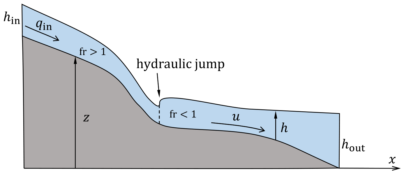
Figure 2.
Typical evolution of the loss history (left) and the corresponding loss weights history (right).
Figure 2.
Typical evolution of the loss history (left) and the corresponding loss weights history (right).
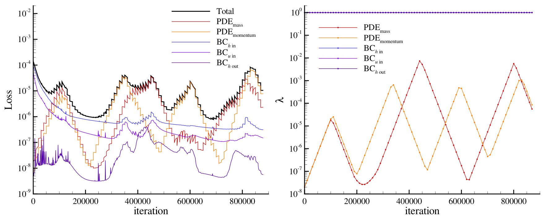
Figure 3.
A map of the Mzymta River basin (obtained from Google Earth digital topographic data)
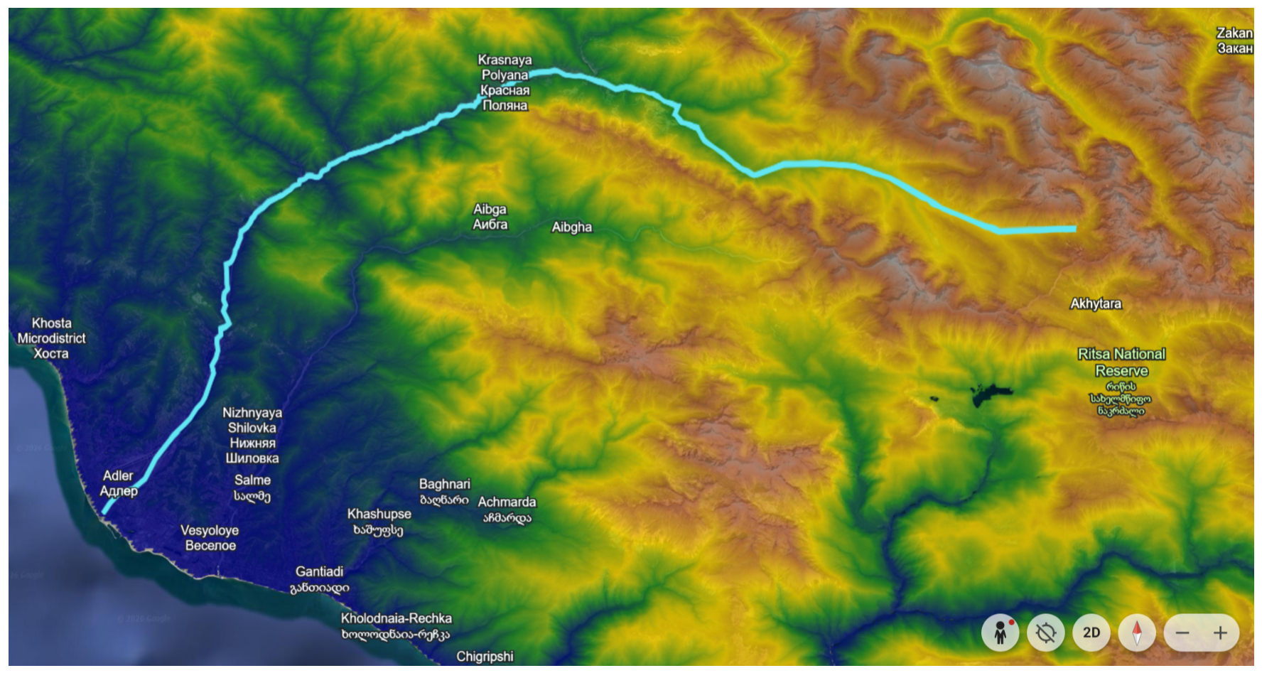
Figure 4.
The profile (black) of the Mzymta River, the smoothed profile (red), and the slope (blue) for the full-scale problem (left) and a short river reach for detailed modeling of the hydraulic jump (right)
Figure 4.
The profile (black) of the Mzymta River, the smoothed profile (red), and the slope (blue) for the full-scale problem (left) and a short river reach for detailed modeling of the hydraulic jump (right)
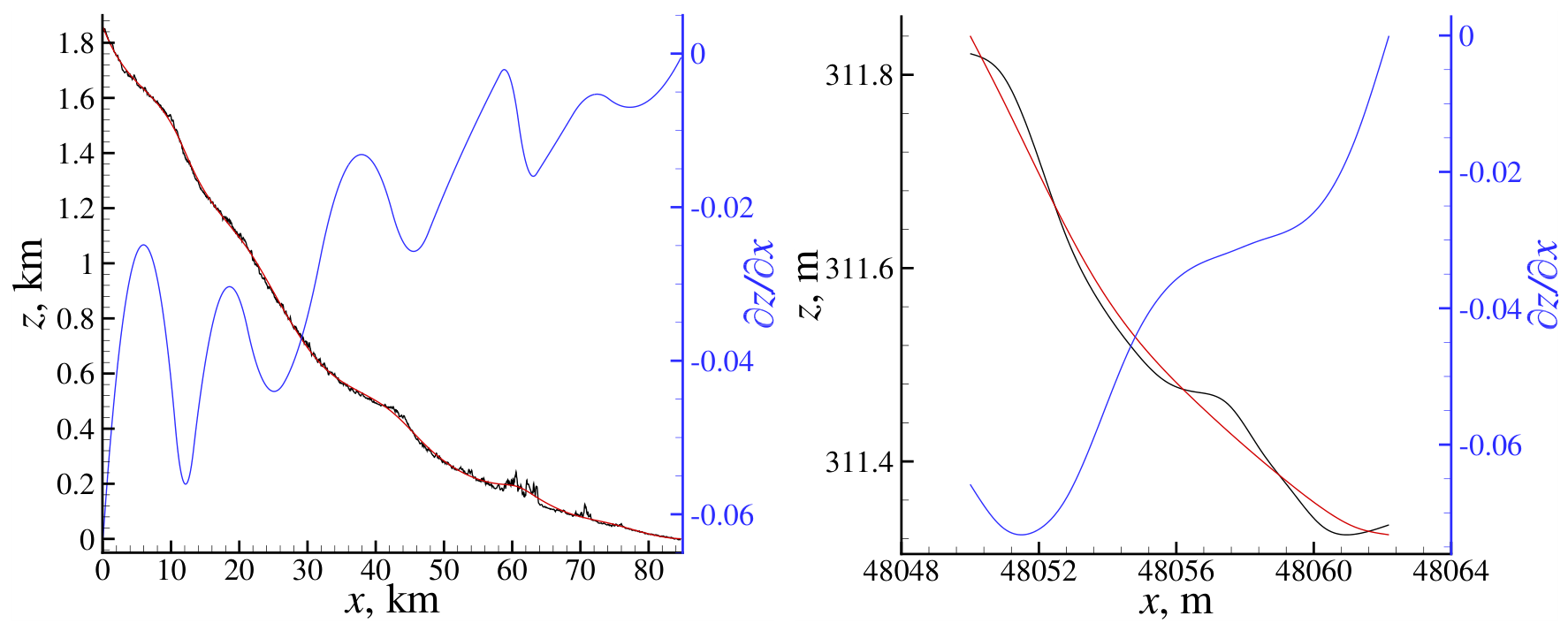
Figure 5.
Time series of water levels and discharges at several hydrological gauging stations on the Mzymta River over the period from 01.06.2023 to 31.08.2023.
Figure 5.
Time series of water levels and discharges at several hydrological gauging stations on the Mzymta River over the period from 01.06.2023 to 31.08.2023.
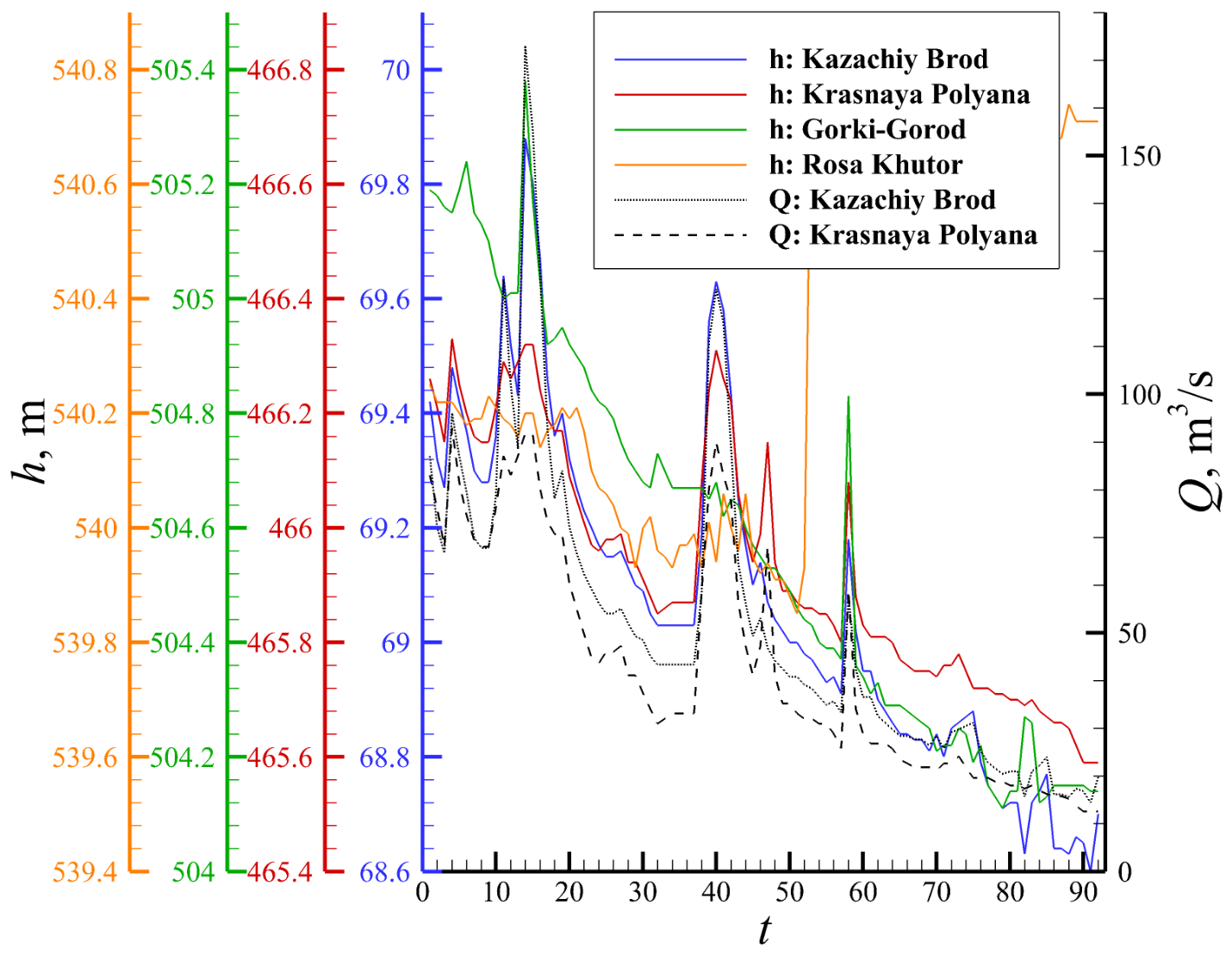
Figure 6.
Depth profiles in the full-scale steady-state problem: critical depth (black dashed), normal depth (black solid), computed using PINNs (red solid) and the RK4 method with downstream integration (blue right triangles) and upstream integration (violet left triangles) depending on the flow regime.
Figure 6.
Depth profiles in the full-scale steady-state problem: critical depth (black dashed), normal depth (black solid), computed using PINNs (red solid) and the RK4 method with downstream integration (blue right triangles) and upstream integration (violet left triangles) depending on the flow regime.
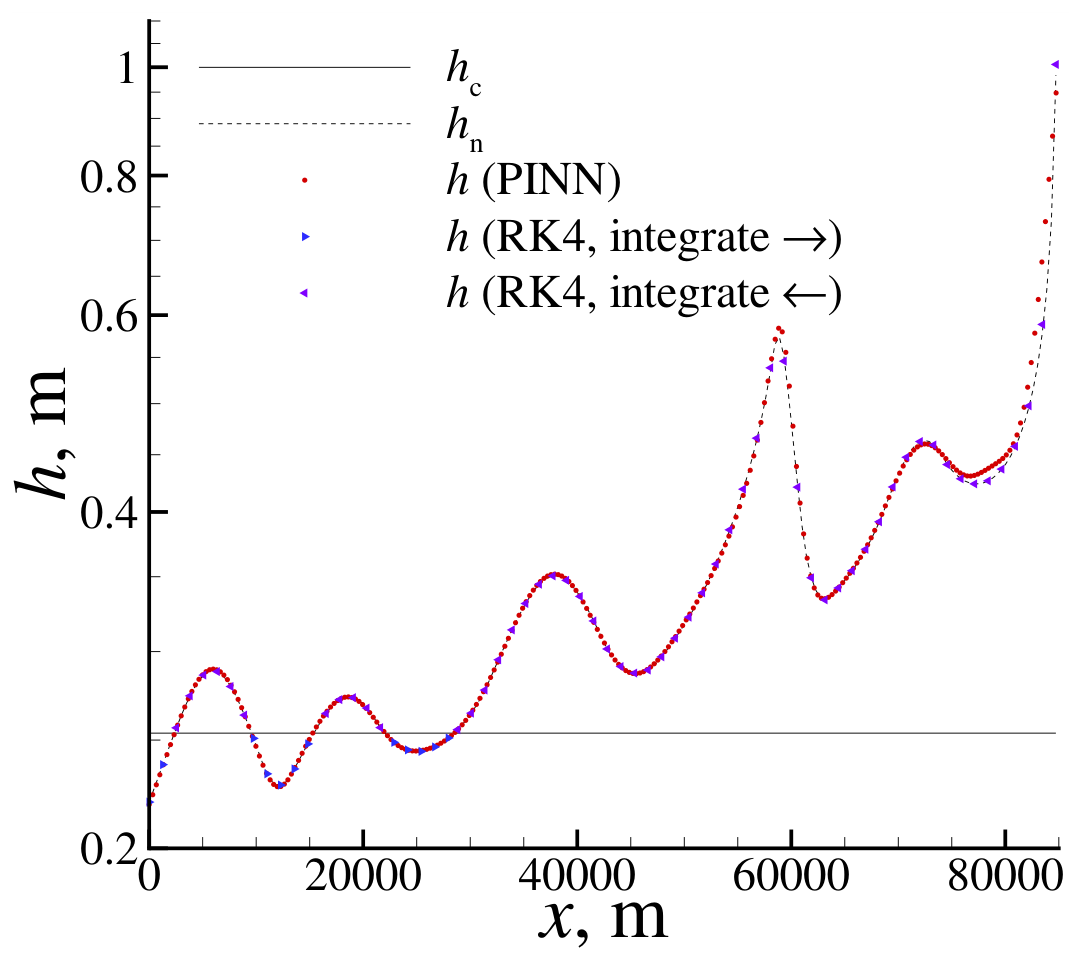
Figure 7.
Distribution of the water depth h (left) and water discharge Q (right) and the characteristic curves (directed lines) for the non-stationary full-scale problem with a sinusoidal discharge.
Figure 7.
Distribution of the water depth h (left) and water discharge Q (right) and the characteristic curves (directed lines) for the non-stationary full-scale problem with a sinusoidal discharge.
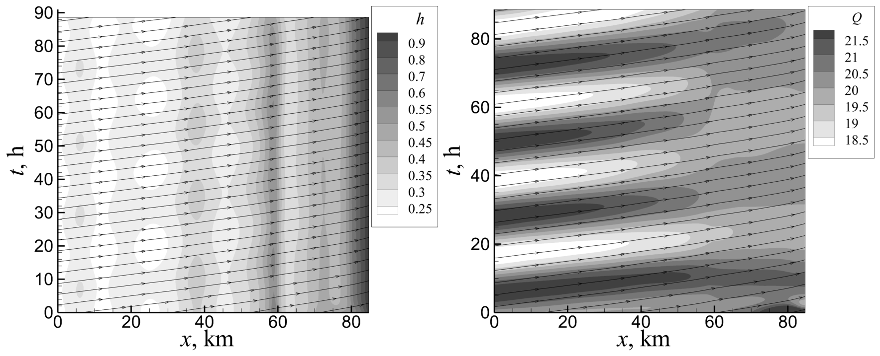
Figure 8.
The non-stationary full-scale problem: depth distribution h (z-axis) and Froude mask ( – white, – blue) over the coordinates (left) and the x-projection (red solid lines) of the depth compared to the normal and critical depth (right).
Figure 8.
The non-stationary full-scale problem: depth distribution h (z-axis) and Froude mask ( – white, – blue) over the coordinates (left) and the x-projection (red solid lines) of the depth compared to the normal and critical depth (right).
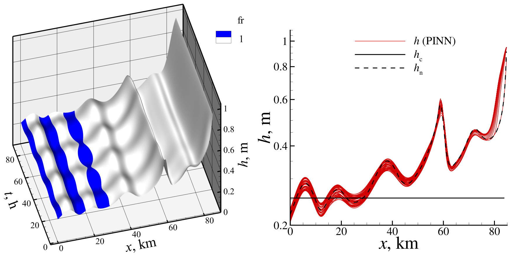
Figure 9.
Depth profiles obtained for the steady-state problem with a hydraulic jump: critical depth (black solid curve), normal depth (black dashed curve), RK4 solution (blue right-pointing triangles for integration in the downstream direction, and violet left-pointing triangles for integration in the upstream direction), PINNs solution without regularization (red dashed curve) and regularized PINNs (red solid curve). Additionally the regularization term (orange solid curve) is shown.
Figure 9.
Depth profiles obtained for the steady-state problem with a hydraulic jump: critical depth (black solid curve), normal depth (black dashed curve), RK4 solution (blue right-pointing triangles for integration in the downstream direction, and violet left-pointing triangles for integration in the upstream direction), PINNs solution without regularization (red dashed curve) and regularized PINNs (red solid curve). Additionally the regularization term (orange solid curve) is shown.
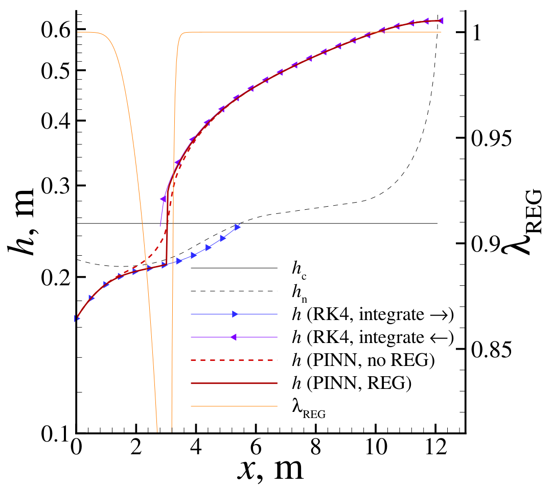
Figure 10.
Distribution of the water depth h (left) and water discharge Q (right) over the coordinates for the non-stationary hydraulic jump problem.
Figure 10.
Distribution of the water depth h (left) and water discharge Q (right) over the coordinates for the non-stationary hydraulic jump problem.
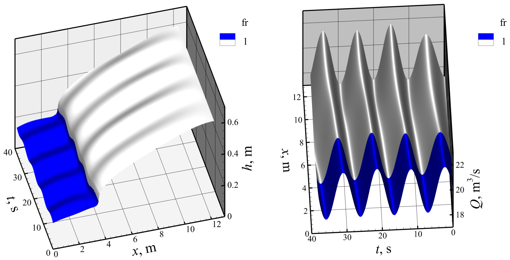
Figure 11.
Distribution of the water depth h solved by non-regularized (left) and regularized (right) PINNs in the non-stationary hydraulic jump problem in various time moments compared to the stationary hydraulic jump problem.
Figure 11.
Distribution of the water depth h solved by non-regularized (left) and regularized (right) PINNs in the non-stationary hydraulic jump problem in various time moments compared to the stationary hydraulic jump problem.
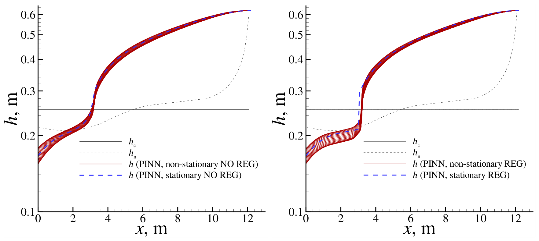

Table 1.
Basic parameters of the simulation.
| Parameter | Value | Source |
|---|---|---|
| g | 9.81 m/ | Real Data |
| W | 50 m | Representative width of the Mzymta River |
| Sl | 0.0218 | Real Data, average slope of the Mzymta River |
| L | 84744 m | Real Data, the length of the Mzymta River from the Kardyvach Lake to the Black sea |
| H | 0.3 m | Real Data, characteristic depth at the hydrological gauging station in Krasnaya Polyana (Figure 5) |
| Q | 20 /s | Real Data, characteristic discharge at the hydrological gauging station in Krasnaya Polyana (Figure 5) |
| q | 0.4 /s | |
| U | 1.32 m/s | |
| n | 0.05 s/ | or the Table in [58] |
Table 2.
Numerical parameters of the model.
| Parameter | Value |
|---|---|
| Training time | 1-12 hours |
| Network width | 64 neurons |
| Network depth | 3-6 layers |
| Activation function | Swish (SiLU) |
| Collocation points (stationary) | 1000 |
| Boundary points (stationary) | 1 |
| Collocation points (non-stationary) | 40000 |
| Boundary and initial points (non-stationary) | 1000 |
| Optimization method | Adam |
| Learning rate | – |
| Loss weights for BC and IC | 1 |
| Loss weights for PDE | – |
Disclaimer/Publisher’s Note: The statements, opinions and data contained in all publications are solely those of the individual author(s) and contributor(s) and not of MDPI and/or the editor(s). MDPI and/or the editor(s) disclaim responsibility for any injury to people or property resulting from any ideas, methods, instructions or products referred to in the content. |
© 2026 by the authors. Licensee MDPI, Basel, Switzerland. This article is an open access article distributed under the terms and conditions of the Creative Commons Attribution (CC BY) license (http://creativecommons.org/licenses/by/4.0/).
Copyright: This open access article is published under a Creative Commons CC BY 4.0 license, which permit the free download, distribution, and reuse, provided that the author and preprint are cited in any reuse.