

Submitted:
02 September 2026
Posted:
03 September 2026
You are already at the latest version
Abstract
Graph neural networks have shown strong potential for learning structural representations of biological networks. However, repeated message passing may blur local structural signals that are relevant for motif- and graphlet-based analysis. This paper investigates multilabel graphlet classification in protein-protein interaction networks to test whether GNNs can serve as reliable structural indicators for motif mining. We focus on two central design choices of message-passing neural networks: network depth, which determines the range of propagated neighborhood information, and neighborhood aggregation, which determines how this information is combined. We compare mean, max, and sum aggregation across increasing message-passing depths and across input feature sets with different levels of structural informativeness. Dropout and batch normalization are considered as additional architectural factors. The resulting models are evaluated using multi-label classification metrics alongside homophily measures and Jensen-Shannon divergence to analyze how label distribution patterns impact prediction performance. Our approach acknowledges the structural limitations of GNNs but seeks to determine if they can serve as reliable "hints" for the presence or absence of graphlets. To connect graphlet prediction with motif discovery, we further include a post-hoc probability-guided motif search in which predicted graphlet probabilities are used to prioritize candidate regions for deterministic motif detection. The study provides an empirical analysis of how depth, aggregation, and feature informativeness interact in motif-oriented graph representation learning.
Keywords:
deep learning
; graph representation learning
; graph neural networks
; multilabel classification
; network motifs
; graphlets
; subgraph matching
1. Introduction
Graphs are powerful tools for modeling real-world systems, especially in biology. Driven by growing interest in network biology, extensive cellular networks – such as transcriptional, metabolic, and protein-protein interaction maps – have already been characterized for numerous model organisms, most notably Escherichia coli and Saccharomyces cerevisiae [53]. In Protein-Protein-Interaction (PPI) networks nodes are proteins and edges correspond to physical bindings between them, forming what is known as the “interactome” [15,19,31,33,50,62]. To reconstruct these interactomes, researchers primarily combine literature-curated data, computational predictions, and systematic experimental techniques like yeast two-hybrid (Y2H) assays and affinity purification mass spectrometry (AP/MS) [41,48,62]. Unlike regulatory networks, the edges in PPIs are undirected, representing mutual, non-causal interactions between protein pairs [42,53]. The local structure of a network around a node can reveal important biological information. These localized wiring patterns are typically quantified by counting how frequently a node participates in so-called graphlets – small induced subgraphs [56]. A related concept, motifs, was introduced in 2002 as small subgraphs that occur more frequently than expected in randomized counterparts [15,31,38,45,47,57]. In contrast to graphlet-based approaches that rely on raw frequency vectors, motif analyses build on statistical significance profiles. Each subgraph is assigned a significance score based on its overrepresentation relative to a null model [37,38,45]. Functional modules such as protein complexes and signaling pathways are encoded as subgraphs within the interactome. These modules mediate enzymatic reactions, signal transduction and cellular decision-making [22,35,37]. However, identifying or counting subgraphs within large networks is computationally challenging: subgraph isomorphism is NP-indeterminate, and determining exact frequency becomes intractable as network size increases [3,20,43].
Motif discovery algorithms can be broadly divided into two main categories: subgraph census (exhaustive search) and subgraph sampling (approximate counting) [45,57]. The subgraph census approach aims to determine the exact frequency of all subgraphs of a certain size k that occur within the input network G. Due to the combinatorial nature of subgraph enumeration and the computational cost of subgraph isomorphism checking, this method becomes infeasible for large graphs. Popular tools implementing exhaustive search include: MAVisto, NeMoFinder and Kavosh [45,57]. Sampling-based algorithms estimate motif frequencies by drawing a large number of random subgraph samples of size k from the input network. Sampling methods are often used when motif detection is applied exploratorily, or when full enumeration is computationally infeasible. Notable implementations include: MFinder [4] and FANMOD [54]. Analytic motif counting methods aim to estimate motif frequencies mathematically. Two major techniques are matrix-based and decomposition-based counting. Matrix-based methods leverage combinatorial properties to derive linear relationships between subgraphs of different sizes [23,45]. The result is a system of linear equations that can be solved using matrix operations. Tools like ORCA [23] and JESSE [36] use such systems to compute graphlet counts efficiently without direct enumeration of all instances. Decompostion-based methods break down each motif into structural primitives, such as shared neighbors, wedge patterns, or overlapping triangles. By computing the frequency of these smaller building blocks, the algorithm infers the total count of larger subgraphs. However, for large biological networks, even state-of-the-art tools can require hours or even days to compute motif frequencies [23,45].
While graph neural networks (GNNs) are powerful tools for general node classification, their theoretical and empirical limitations in capturing local topological structures – such as subgraph isomorphism and motif counting – remain a critical challenge [13,59] Literature suggests that standard message-passing architectures are inherently limited by their equivalence to the Weisfeiler-Lehman (WL) graph isomorphism test, preventing them from reliably distinguishing specific graph patterns or counting induced subgraphs of size three or more [13]. This raises a fundamental question: Can GNNs generate distinct embeddings for nodes with different roles in a subgraph to accurately classify their membership, even if exact counting remains theoretically unreachable? To investigate this, we cast motif and graphlet detection as a multi-label node classification problem using GraphSAGE [21]. Our approach acknowledges the structural limitations of GNNs but seeks to determine if they can serve as reliable “hints” for the presence or absence of graphlets. By using predicted probabilities to guide a rule-based subgraph detector, we bridge the gap between representation learning and deterministic mining, evaluating whether GNNs can provide a useful complement to traditional search. Crucially, we move beyond the coarse homophily-heterophily dichotomy, analyzing the interplay between feature informativeness – ranging from constant scalars to spectral moments – and topological properties.
This work provides a comprehensive empirical investigation into motif-oriented graph representation learning through the following key contributions:
- Framing Motif Detection as a Multilabel Task: We utilize isomorphism-dependent downstream tasks to probe the expressiveness limits of message-passing architectures, testing the ability of GNNs to distinguish node roles within larger structures.
- Systematic Architectural Grid Search: Through a large-scale grid search of 396 configurations, we isolate the impacts of network depth, aggregation operators, and normalization. We demonstrate that performance degradation in deep models is driven by a complex interplay between feature informativeness and topological convergence, rather than oversmoothing alone.
- Fine-Grained Topological Analysis: We analyze how embedding separability and node homophily evolve across neighborhoods, offering a nuanced explanation for performance fluctuations that traditional “oversmoothing” narratives often overlook.
- Transductive vs. Inductive Generalization: By evaluating across both settings, we demonstrate that topology-aware feature engineering (such as spectral moments) enables GNNs to learn effectively even from minimal or dummy feature representations.
- Probability-Guided Hybrid Detectors: Recognizing that GNNs cannot perform exact subgraph matching, we introduce a post-hoc, probability-guided search. This approach leverages GNN outputs to prioritize candidates for rule-based detectors, investigating whether this hybrid pipeline can learn to locate structural patterns efficiently. While our analysis reveals that high label homophily in protein-protein interaction networks limits the reduction of computational complexity, the resulting precision highlights the potential of GNNs as structural indicators for motif mining.
Motif mining typically involves an additional significance testing step by comparing raw counts against randomized versions. In this work, we bypass explicit significance testing, investigating whether GNNs can directly learn representations to guide subgraph search. The remainder of this paper is organized as follows. Section 2 establishes the theoretical framework, detailing graphlet degree distributions, message-passing mechanics, and node-level feature representations, followed by our multi-label classification and homophily formalisms. Section 3 outlines the experimental setup, describing the dataset properties, label binarization scheme, and full hyperparameter search space. Section 4 presents the empirical findings across both transductive and inductive settings, examining the interplay between feature quality, aggregation operators, network depth, and oversmoothing, alongside the performance of our post-hoc probability-guided motif search. Section 5 discusses the broader implications of embedding separability, topological limitations, and computational trade-offs and concludes the study with directions for future research.
2. Theoretical Framework and Modeling Approach
2.1. The Rudiments of Graph Theory
Motif finding inherently requires detecting whether target structures exist within a larger network via subgraph isomorphism. In this section we first establish the foundational graph constructs that govern these matching tasks. A graph models entities as vertices and their pairwise relationships as edges , where two vertices are adjacent () if [2]. At the local level, local message passing in GNNs operates over the open neighborhood , whose size determines the vertex degree [2]. To enable matrix-based GNN operations, G is compactly represented via its adjacency matrix [2,9], where:
Building upon this matrix representation, motif discovery fundamentally relies on solving the NP-complete subgraph isomorphism problem [7,45] to identify whether a target motif H appears within G. Formally, is a subgraph of if and . In the literature, motif mining is defined in subtly different ways depending on whether the target patterns are treated as general (non-induced) or induced subgraphs. Formally, given a subset of vertices , the induced subgraph is defined as:
To differentiate fine-grained structural positions within these induced motifs, vertex roles are classified via graph symmetries. An automorphism of a graph is a self-isomorphism, defined as a bijection that preserves edge connectivity:
The set of all such bijections forms the automorphism group . This group induces an equivalence relation over V, partitioning the vertex set into equivalence classes referred to as orbits [2,45].
In the remainder of this work, we use the terms vertex (plural: vertices) and node interchangeably.
2.2. Graphlet Degree Distribution
Formally, a k-graphlet denotes a small, connected, and non-isomorphic induced subgraph g comprising a subset of k interconnected nodes in G [34,45]. To account for structural symmetries within these subgraphs, automorphism orbits partition the nodes of a graphlet into equivalence classes, grouping together topologically equivalent positions that can be interchanged without modifying the overall graphlet structure [2,45,56]. As the subgraph size k grows, the combinatorial diversity of distinct undirected graphlets alongside their respective automorphism orbits grows exponentially. For instance, while a size of yields merely 2 unique graphlets and 3 orbits, increasing the order to expands this space to 21 graphlets with 58 distinct orbits, eventually scaling to more than two million orbits when considering graphlets of order [23,43].
The graphlet degree vector (GDV) of a node encodes how many times a node touches each graphlet at a particular automorphism orbit [23,43,45,56]. In this context, the node degree can be interpreted as a special case – namely, orbit o(0) [45]. For any given node, the total count for a specific graphlet is the sum of the orbit counts associated with that graphlet [43,56]. These vectors can be aggregated across the graph to form the graphlet degree distribution matrix , where entry indicates the number of nodes that appear i times in orbit j [45,62]. The computational complexity of counting all graphlets of size k is , where d is the maximum degree of the graph G. Due to the combinatorial explosion, the computation for graphlets is usually restricted to nodes. [11,34,60]. Figure 1 shows graphlets of size up to five nodes.
2.3. Deep Learning on Graphs and Information Diffusion Mechanism
Graph Neural Networks (GNNs) leverage both the graph structure and node features to learn a representation vector for individual nodes or entire graphs . Modern GNNs commonly follow a neighborhood aggregation scheme. After k iterations, the node embedding captures the structure of its k-hop neighborhood [18,20,28,58].
Formally, the general update rule at the k-th layer of a GNN is given by:
or equivalently:
The AGGREGATE function collects information from the set of neighboring nodes , resulting in a combined message (Figure 2). Then, this message is passed to the UPDATE function, which combines it with the current embedding of node u to produce the new representation [18,20,28,58,59].
The initial embeddings at are set to the input features for each node:
After running K iterations of the message passing process, the final node embedding is obtained as:
The neighborhood aggregation operation is fundamentally a set function. We are given a set of neighbor embeddings and must map this set to a single vector . A GNN must distinguish different multisets of node features – otherwise, it will map structurally different neighborhoods to the same embedding. The more discriminative the aggregation function is with respect to different multisets, the higher the representational power of the GNN [58].
Figure 3 illustrates this issue: although the graph structures around node v differ, simple aggregation schemes like mean or max assign the same embeddings to v and . These functions fail to capture multiplicities in the multiset of neighbor features – they reduce the multiset either to its average or to its maximum element. This leads to an inability to distinguish graphs that differ only in neighborhood cardinality or composition.
2.4. Node-Level Features
Instead of computing embeddings for each node individually, GraphSAGE learns a function that can generate node embeddings by aggregating information from local neighborhoods [14]. This function can generalize to new nodes by leveraging node features. The method can also be applied to graphs without explicit node features, relying on structural signals instead. Node attributes are typically represented as a feature matrix , where is the number of nodes and m is the dimensionality of the feature vectors. Basic statistics such as the degree of a node are frequently used as features in traditional node classification tasks. Further informative descriptions can be derived from the centrality measures, which quantify different aspects of a node’s importance within the graph structure [20,27].
Centrality measures estimate how important a node or edge is for maintaining connectivity or facilitating information flow [20,27]. The concept of centrality depends on the specific type of influence under investigation. Three widely used measures include:
- Degree centrality: describes the number of direct connections a node has.
- Betweenness centrality: describes how often a node lies on the shortest paths between other nodes.
- Closeness centrality: defined as the inverse of the average shortest path from a node to all others.
2.5. Cospectrality and Eigen Decomposition Pruning (EDP)
Two graphs are cospectral if they share the exact same adjacency eigenvalues. While all isomorphic graphs are inherently cospectral, the converse does not necessarily hold [2,55]. Spectral similarity is based on matrix similarity: two matrices and are similar if there exists an invertible matrix P such that:
If and are similar, then they share the same eigenvalues [2,9,16,55].
Verifying cospectrality does not require full eigenvalue decomposition. Instead, it is sufficient to demonstrate that the traces of powers of their adjacency matrices are equal across all walk lengths::
Here, corresponds to the total number of closed walks of length k in the graph. Thus, and are cospectral if and only if for each , the total number of closed walks of length k in equals that in [2].
Building on spectral properties, Moayed et al. [40] introduced Eigen Decomposition Pruning (EDP) to pinpoint candidate subgraphs in large networks that potentially match a given query motif. The method is based on the following key concepts:
- Neighborhood Pattern : is defined as the structural signature of the k-hop neighborhood around a node u.
- Neighborhood Subgraph : the induced subgraph containing all nodes and edges within a distance k from a node v.
-
Local Laplacian Matrix (LLM):where D and A denote the degree and adjacency matrices of the induced subgraph, respectively.
Inspired by the EDP method, we approximate the Laplacian spectrum of each node’s 2-hop egonetwork using the ApproxSpectralMoment algorithm proposed by [16,26]. This method estimates the eigenvalue distribution by simulating 10.000 random walks of length 20 and computing the proportion of closed walks, which reflect the spectral properties of the transition matrix. For each egonetwork, we repeat the estimation 20 times and average the results. From the resulting spectra, we extract the first six spectral moments per node. Since the first moment is zero we use moments 2 - 6 as features. These moments are isomorphism-invariant, meaning they remain unchanged for structurally equivalent graphs [16]. We use the intersection of the set of spectral features of the query graph and subgraphs as a clue of similarity.
This spectral approach is further validated by Jin and Zafarani [25], who established formal equivalences between low-order spectral moments and fundamental node attributes (e.g., degree and clustering coefficient) as well as motif patterns such as edges, wedges, triangles, and cycles.
2.6. Multilabel Classification
Multilabel classification is a generalization of binary classification to multiple independent labels [44]. Each instance is associated with a subset of labels so the dataset becomes:
The binary relevance method trains binary classifiers , where each classifier is responsible for predicting the presence or absence of its corresponding label [44,63]. In the multilabel setting, the following F1 variants are commonly applied: micro, macro and instance-based averaging [30,44]. In practice, each label can be assigned a separate decision threshold. Here, we assume a fixed probability cutoff (e.g., 0.5) to make the approach more reproduceble.
2.7. Graph Homophily
Label homophily quantifies the similarity among neighboring nodes based on their label distributions. Graphs are typically categorized as either homophilic or heterophilic [18,39,63].
The node homophily is defined as the average proportion of edge-label consistency of all the nodes [18,39,63]. Formally, we have:
where is the node set and is the neighbor set of node v. , denote the labels of nodes v and u, respectively. Gong et al. [18] extend this definition to the k-hop neighbors to measure high-order homophily:
where represents the k-hop neighbors of v. Both node and edge homophily range from [0,1], and high homophily indicates low heterophily, and vice versa [18].
Zhao et al. [63] argue the basic homophily definition can not be directly used in the multi-label graph datasets, as each node can have more than one label. Further, they define multi-label label homophily as follows:
Given a multi-label graph G, the label homophily h of G is defined as the average of the Jaccard similarity of the label set of all connected nodes in the graph:
2.8. Oversmoothing in Graph Neural Networks
When striving for generalization, it is important to account for oversmoothing – a phenomenon where deep GNNs tend to produce almost constant representation, independent of the original node-feature distribution, which can ultimately lead to a loss of discriminative power [5,6,10,12,17,32,46]. Formally, let be the matrix of node embeddings after ℓ message-passing layers in a GNN, where n is the number of nodes and d is the hidden dimension. Consider a similarity function , where is the space of all possible embedding matrices. We say that a deep GNN experiences oversmoothing if
where c is a constant indicating a collapse of embeddings [6,39]. This creates an almost constant representation, independent of the original node-feature distribution [5,6,10,12,17,32,46].
In the literature, drop in test accuracy in deep GNNs is frequently blamed on oversmoothing, following the hypothesis that once embeddings collapse into a trivial space, nodes become hard to separate, leading to a decline in performance [6,10]. To pin this down, recent studies have worked on more precise definitions of oversmoothing using metrics like graph Dirichlet, cosine similarity, or mean-average distance (MAD) [6,46]. To determine how far information needs to propagate, Alon and Yahav [5] define a ’problem radius’ r, which is usually approximated by tuning the number of layers K. In practice, since most nodes in a connected component are within a few hops of each other, GNNs with just two or three layers are often sufficient to achieve competitive results [5,32].
While Chen et al. [12] attribute oversmoothing to the over-mixing of signals – where inter-class interactions introduce harmful noise and impair representation separability – the nature of our task introduces a unique constraint. Because our target labels are inherently tied to the network topology, a high local label density is practically unavoidable. Consequently, we hypothesize that this task requires only a short receptive field, as the underlying graphlet structures span a maximum neighborhood of two hops. Nonetheless, to examine how GNN performance scales with network depth, we evaluate architectures ranging from 2 to 12 layers – extending one layer beyond the diameter of the interactome. We systematically investigate how label homophily varies across different graphlets as network depth increases, and how these structural changes impact performance. In the literature, various architectural techniques – such as residual connections, normalization layers, or gating mechanisms – are commonly used to mitigate oversmoothing and preserve local distinctions [6,17,46]. Building on this, we specifically incorporate batch normalization and dropout into our models to stabilize training and counteract embedding collapse across these varying depths.
3. Experimental Setup
3.1. Dataset Description
In this study, we used the human proteome-scale PPI network published by Thul et al. [50], accessible via the Human Cell Map. The network was modeled as an undirected graph, and for all subsequent analyses, we extracted its greatest connected component (GCC) containing 7185 nodes and 59968 edges. For training and validation in the inductive setting, we employed the BioSNAP human PPI dataset [1], which contains 24 biologically meaningful networks.
3.2. Label Distribution
ORCA provides a 73-component graphlet GDV for each node in the graph. To establish our ground truth, we convert the GDV into a count vector and binarize it to indicate simply whether a node participates in a given graphlet or not. To quantify class prevalence, we define the normalized label frequency by dividing the count of active nodes by the total number of nodes for each of the 29 labels. Figure 4 illustrates the normalized label frequency for graphlets 1 through 29 (orbit 0 and graphlet 0, corresponding to a simple edge, are omitted). The normalized label frequency exhibits pronounced class imbalance, an inherent consequence of explicitly searching for induced subgraphs.
3.3. Model Architecture and Hyperparameter Space
Each GNN layer in this framework can be defined as:
where is the k-th layer embedding of node v, , are trainable weights, and is the local neighborhood of v. We stack multiple layers and define the full model configuration as the Cartesian product of the following intra-layer design options:
- Aggregation function:
- Activation function:
- Batch normalization:
- Dropout rate:
- Hidden dimension:
We evaluate architectures ranging from 2 to 12 layers. This results in a total of unique configurations, each of which was trained for 1000 epochs per feature set. To ensure robustness and account for initialization variance, every configuration was evaluated using five different random seeds. All models were trained using the Adam optimizer with a fixed learning rate of 0.001, complemented by early stopping and weight decay. We used GraphSAGE as the base model for its inductive capabilities [14,21]. The simulation environment was implemented in Python, using widely adopted graph learning libraries such as PyTorch Geometric and NetworkX, together with standard packages like NumPy, Matplotlib, and Pandas. For the multilabel classification task, we used the BCEWithLogitsLoss function, which combines a Sigmoid layer and the binary cross-entropy loss in a single class. This enables the model to make independent binary predictions for each graphlet membership per node.
4. Results
4.1. Results Transductive Setting
4.1.1. Grid Search and Effect of Varying Feature Quality
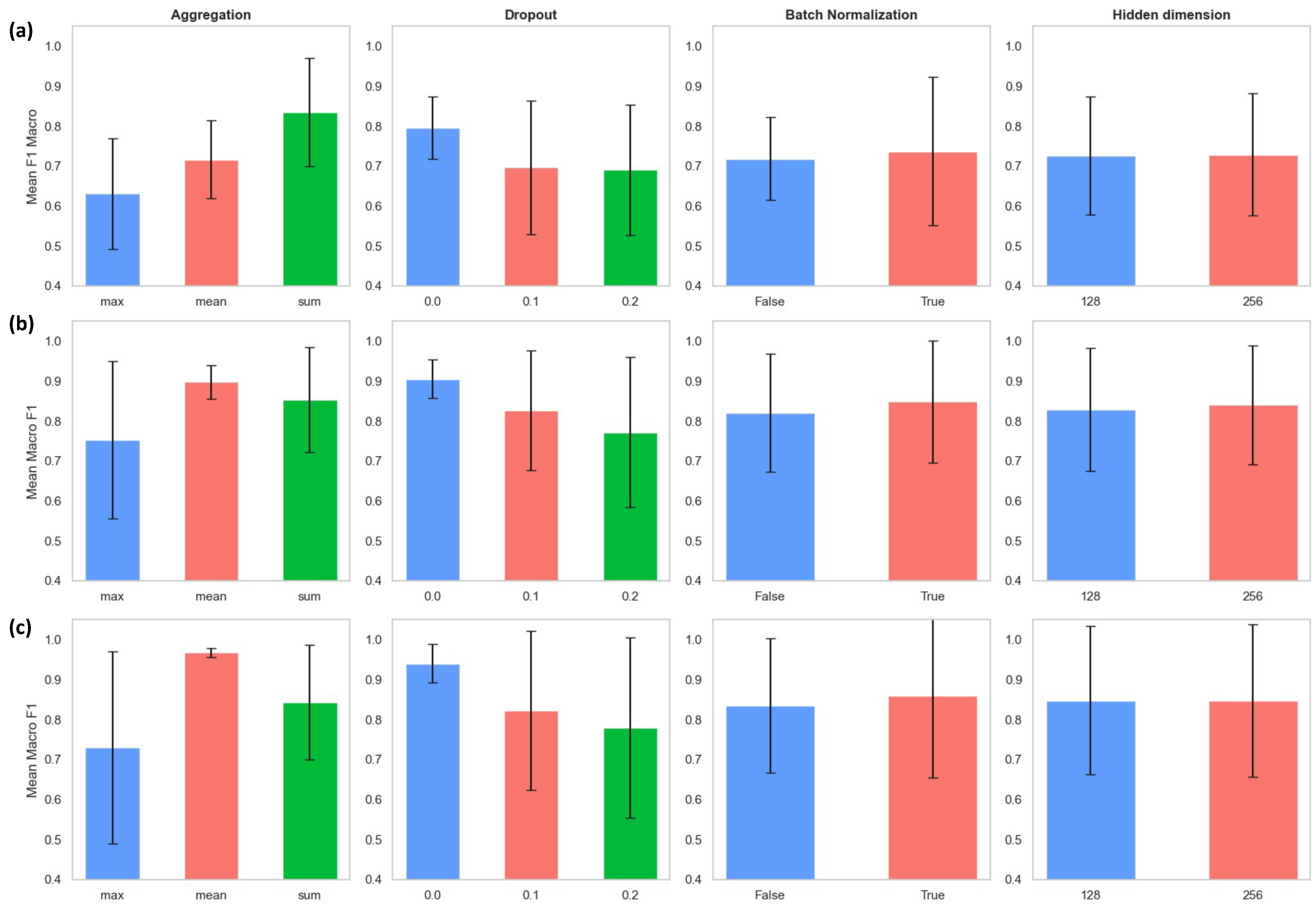
To analyze the mechanics of model depth and feature representations, we conducted a full grid search across 396 architectural configurations over 5 random seeds. Figure 6 reports the mean Macro-F1 performance across all feature sets, where error bars denote the standard deviation across configurations sharing the same design choices. As illustrated in Figure 5, the decline in performance with increasing layer depth is strongly dependent on the choice of the aggregation operator and the utilized feature set. Specifically, our results demonstrate that the max, mean, and sum strategies react differently to increased depth, suggesting that the observed performance degradation is not merely a consequence of the number of layers (i.e., ’excessive smoothing’), but rather a result of the specific mechanism of information aggregation and its interaction with the input features.
In alignment with Figure 5, performance fluctuates heavily with network depth. This variance is reflected in the large standard deviations observed in Figure 6, particularly for deeper architectures where representation collapse occurs. As the network depth increases from 2 to 12 message-passing layers, models consistently suffer from degradation due to overfitting and embedding collapse. However, the severity of this performance drop varies significantly depending on the choice of aggregation operator and feature informativeness:
- Sum Aggregation and Expressiveness Trade-offs: While sum aggregation enhances expressiveness for uninformative or dummy features (e.g., constant scalar) by preserving multiset cardinalities, it becomes inherently unstable with increasing depth. Because the receptive field grows exponentially with node degree, summing unnormalized neighbor features leads to an uncontrolled accumulation of ones, causing training loss to surge drastically and remain stuck at high levels.
- Hidden Dimensions and Feature Similarity: Model performance remains virtually on par across different hidden dimensions (128 vs. 256).
- Dropout Impact: By randomly zeroing out features during message passing, dropout disturbs consistent neighborhood aggregation. Under sum aggregation, this introduces violent amplitude fluctuations, whereas under max aggregation, it severely exacerbates information loss.
- Batch Normalization: The impact of Batch Normalization fluctuates strongly based on the aggregation function. While it acts as a crucial stabilizer that prevents gradient explosion under sum aggregation and mitigates over-smoothing, its interaction with max and mean aggregations shows varying dynamics across hyperparameter choices (see Appendix B for details).
Figure 6.
Mean macro F1 across different feature sets. Each subpanel reports the results of a full-grid search over architectural design dimensions: aggregation function, dropout rate, batch normalization, and hidden dimension size. Error bars represent standard deviations across all configurations sharing the same design choice. (a): constant scalar feature set, (b): spectral moments, (c): centralities and clustering coefficient.
Figure 6.
Mean macro F1 across different feature sets. Each subpanel reports the results of a full-grid search over architectural design dimensions: aggregation function, dropout rate, batch normalization, and hidden dimension size. Error bars represent standard deviations across all configurations sharing the same design choice. (a): constant scalar feature set, (b): spectral moments, (c): centralities and clustering coefficient.
To analyze the underlying mechanics of oversmoothing, we examine how feature distributions evolve across network layers. Formally, a GNN reaches a state of complete representation collapse () when its covariance matrix contracts to constant entries, [17]. Under this condition, nodes receive identical pre-activations, ultimately collapsing into uniform embeddings (). As demonstrated in prior work, this uniform state acts as an invariant fixed point of the network dynamics [17]. Driven by strong layer-wise contraction properties, this fixed point behaves as a powerful attractor: even when starting from distinct initial features (), node representations rapidly converge toward zero feature distance () as network depth increases [17].
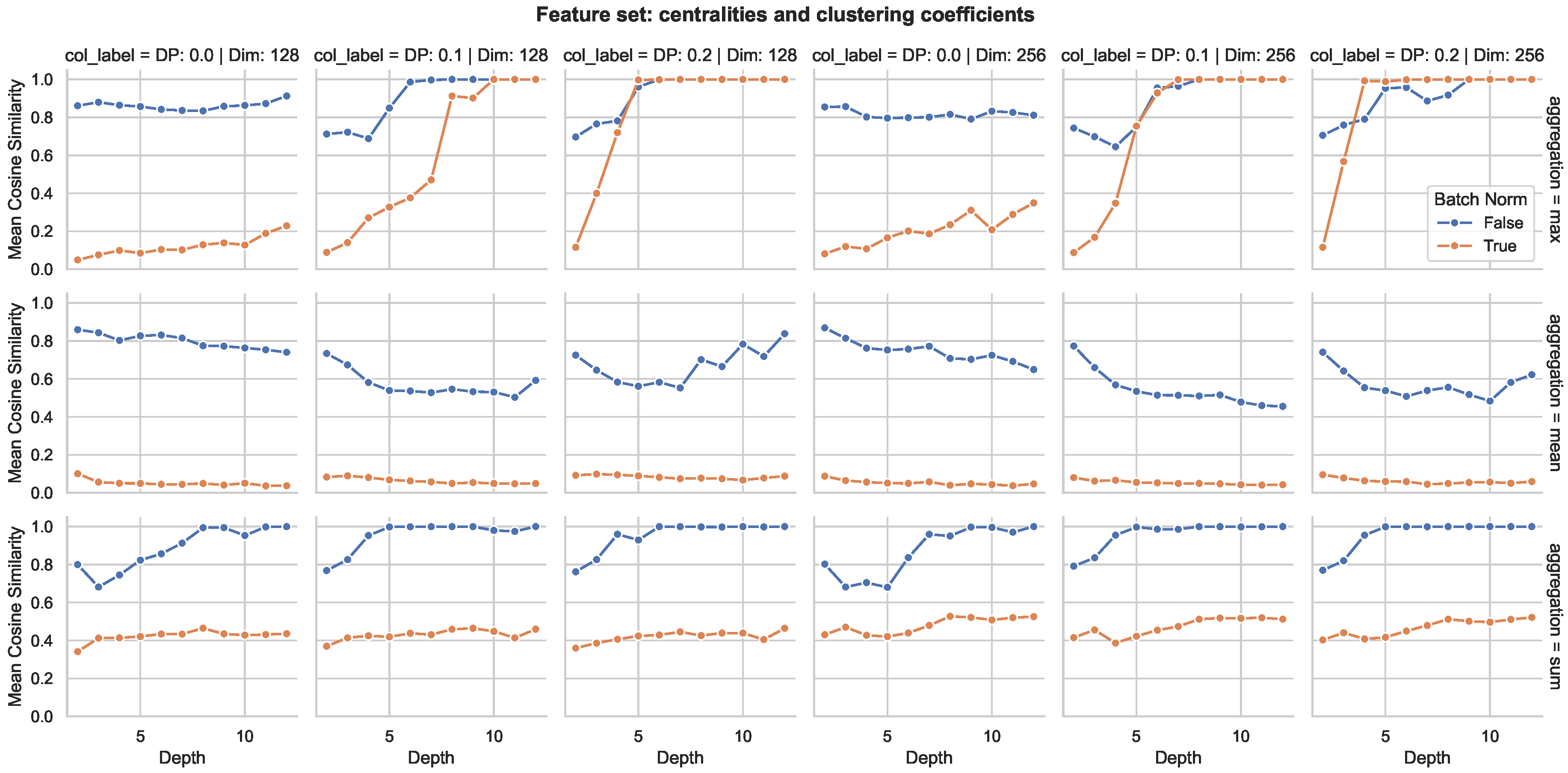
To empirically evaluate this behavior, we recorded the final node embeddings across all evaluated network depths () and computed their pairwise cosine similarities (Figure 7). While several configurations exhibit a steep increase in similarity toward higher depths – indicating severe embedding collapse – our findings show that this effect is highly sensitive to model architecture. In particular, Batch Normalization acts as a vital stabilizer across all aggregation schemes: by re-scaling and re-centering features at each step, it continuously reintroduces variance into the feature space, thereby suppressing oversmoothing and maintaining layer-wise feature separability.
Building upon this theoretical framework, our grid search reveals an intriguing interplay between feature informativeness and aggregation methods:
- Constant Scalar: homogeneous initializations, such as a constant value of 1 assigned to every node, places the network almost directly onto the fixed point, maximally accelerating the collapse of representations.
- Spectral Moments & Centralities: Spectral moments derived from 2-hop ego-networks exhibit highly overlapping neighborhoods due to the interactome’s high clustering coefficient.
- Centralities and Clustering Coefficient: centrality measures paired with the clustering coefficient provide node-specific attributes, offering the highest degree of distinguishability and performing best.
- Aggregation Function:max-pooling proves to be the weakest and most unstable aggregation function, consistently characterized by aggressive information loss and a rapid collapse of representations. sum aggregation acts as a strong contraction driving the network toward the attractive fixed point, though it can theoretically prevent collapse when paired with proper weight variance tuning () [17]. In contrast, mean aggregation excels when paired with informative input features, acting as a stabilizing damper through constant degree normalization.
Finally, introducing dropout modulates this behavior significantly depending on the chosen aggregation scheme. Dropout acts as a regularizer but, in deep GNNs, leads to stochastic feature dropping that accelerates embedding collapse:
- Under sum aggregation, which scales neighbor messages directly by the node degree, dropout breaks the consistent accumulation of signals, resulting in violent amplitude fluctuations and a rapid drift into the attractive fixed point.
- max aggregation, inherently preserves only the dominant neighborhood signal while discarding all alternative features. Consequently, random feature dropping severely compounds this information bottleneck, depriving the network of sufficient variance and causing rapid representation degeneration.
- Conversely, mean aggregation remains robust against dropout disturbances. By dividing by the node degree, it compensates for missing signals and prevents the abrupt breakdown of the information flow, as further evidenced in Figure 7.
For a detailed breakdown of results across varying dropout rates and hidden dimensions, we refer to Appendix B.
Figure 8 reports the graphlet precisions averaged over 5 train/val/test splits, highlighting clear performance variations across both feature sets and aggregation mechanisms. The anticipated failure cases are prominently reflected in the constant scalar setting, where cycles (e.g., ) and clique-graphs () exhibit vanishing precision. Theoretically, these non-isomorphic topologies cannot be distinguished through local feature distributions alone (Figure 3), as they differ strictly in neighborhood cardinality and composition.
Under uninformative inputs, less expressive, non-injective aggregators (e.g., mean or max pooling) map these distinct local neighborhoods onto identical vectors, inducing severe embedding collapse. In contrast, sum aggregation preserves multiset injectivity by accumulating unscaled neighbor signals, thereby retaining neighborhood cardinality and enabling the model to disambiguate subtle structural differences. Beyond these expressiveness limitations, a comparison with the label distribution (Figure 4) reveals that class imbalance further amplifies underperformance, as graphlets with sharply declining precision values are heavily underrepresented in the interactome.
4.1.2. Effect of Label Homophily
A complementary explanation for the precision fluctuations in Figure 8 is oversmoothing, caused by information overmixing across layers. To analyze this, we extend our evaluation to higher-order homophily based on Gong et al. [18], adapting their formulation to our multi-label setting by computing the metric independently for each label across k-hop neighborhoods (). As shown in Figure 9, this reveals distinct topological patterns: graphlets like , , and show low local homophily () that decays rapidly over higher hops. In these regions, nodes aggregate signals from neighbors with different labels, blurring feature boundaries. For graphlet classification, this is worsened by non-induced neighbor connections: nodes within an induced graphlet often connect to non-induced variants of the same motif, pulling in signal from “forbidden” structures. Combined with their low representation in the dataset (Figure 4), this lack of neighborhood consistency and structural noise prevents the model from separating classes effectively, causing sharp precision drops for minority graphlets in deeper networks.
4.2. Results Inductive Setting
4.3. Grid Search and Effect of Varying Feature Quality
To evaluate the model’s ability to generalize to unseen graph structures, we adapted the experimental design for the inductive setting by constraining the network depth to 2 – 4 layers. Table 1 shows the condensed configuration space for the inductive setting. The dataset comprises a heterogeneous collection of BioSNAP and cell-compartment graphs, varying significantly in size and density (see Table A1). To ensure robust generalization, we stratified graphs into three size categories (small, moderate, large) and performed a random 17/8/8 train/val/test split.
Figure 10 presents the hyperparameter landscape across the configuration space. Compared to the transductive setting, the performance profiles appear markedly more stable, as the constraints on network depth effectively prevent the inclusion of severely oversmoothed configurations.
While the qualitative preferences – such as the inherent instability of max aggregation and the sensitivity to feature informativeness – persist, the inductive performance highlights two key observations:
- Optimal Depth: all three feature sets maintain their strong preference for shallow, 2-layer architectures, confirming that depth optimization is an intrinsic property of the feature set rather than a setting-specific artifact.
- Aggregation Dynamics: While sum and mean aggregations perform nearly on par when utilizing informative Spectral Moments and Centralities, the sum operator consistently outperforms mean for Constant Scalar inputs.
Ultimately, the inductive results corroborate the findings from our transductive analysis: by limiting message-passing to a moderate depth, the GNN avoids the performance degradation induced by the attractive fixed point of vanishing feature distance.
The label-wise precision plot in Figure 11 reveals a marked reduction in the performance drops previously observed in the transductive setting. Benefiting from a substantially larger and more diverse pool of training data points, the GNN achieves smoother and more consistent precision profiles across label classes. Nevertheless, the Constant Scalar features continue to exhibit characteristic performance drops across specific failure cases, heavily dependent on the chosen aggregation method. A potential explanation for the observed weaknesses of Spectral Moments comes from the local nature of their computation. Because Spectral Moments are derived from bounded subgraphs (e.g., 2-hop ego-networks), adjacent nodes share a substantial portion of their local neighborhood. Consequently, neighboring nodes receive highly correlated initial feature representations. This spatial overlap renders the representations particularly vulnerable to accelerated oversmoothing during message passing.
4.3.1. Effect of Label Homophily
Table 2 outlines the structural characteristics and Macro-F1 performances across the test graphs, highlighting three core insights into inductive generalization:
- Stable Generalization under High Homophilie: The BioSNAP graphs exhibit exceptionally high label homophily () alongside very low Jensen-Shannon divergences (JSD). Under such extreme homophily, message passing acts primarily as a smoothing operator over aligned labels, mitigating misclassifications from oversmoothing. The minimal Jensen–Shannon divergence confirms that local neighborhood features remain topologically consistent This structural consistency explains why Macro-F1 scores remain constantly high ().
- Impact of Graph Scale and Distribution: While larger BioSNAP networks display near-perfect homophily and homogeneous label distributions, smaller or more structurally diverse graphs – such as Golgi () and Vesicles () – exhibit a noticeable drop in homophily and JSD values. This structural divergence correlates directly with lower Macro-F1 scores, particularly when paired with uninformative Constant Scalar features.
- Robustness of Informative Features: Even in structurally challenging environments, such as the Golgi compartment with a homophily of , Spectral Moments and raw node features maintain remarkable stability. They significantly outperform the Constant Scalar baseline, underscoring that informative feature-engineering effectively mitigates performance losses induced by low homophily.
4.4. Graphlet-Matching Guided by Predicted Probabilities
To complement the GNN predictions, we implement a post-hoc motif detection strategy that explicitly counts motif instances. While classification models indicate whether a node participates in a specific motif, they do not quantify the exact frequency or local context of its occurrence. To address this limitation, we developed custom detectors for each of the 29 graphlets. Obtaining a reliable ground-truth count requires aggregating node-specific information; to this end, we leverage ORCA, which provides the frequency of a node v appearing in a given orbit . Through combinatorial transformations, these orbit counts are converted into graph-wide totals: one can either sum the asymmetric orbit counts across all nodes or utilize symmetric orbit counts adjusted by the number of unique symmetric orbits within the respective graphlet. We restrict our evaluation to graphlets, as detectors repeatedly exceeded time limits for .
Detection is simulated for each feature set using its best-performing configuration based on Macro-F1 score:
- Constant Scalar:
- Spectral Moments:
- Centralities and Clustering Coefficient:
For each graphlet, target nodes exceeding a classification probability threshold of are assigned an anchor role (orbit) based on their local neighborhood. We then extract their 1-hop neighborhood and filter out candidate nodes that violate structural constraints by containing “deal-breaker” edges – connections explicitly prohibited within the target graphlet’s induced subgraph definition (see Figure A4). For a detailed overview of the absolute errors across feature sets and test graphs, see Tables A3–A5 in the Appendix.
Table 3 presents the ground-truth counts computed via ORCA alongside the absolute deviation from our detected counts. Consistent with Figure 8, the absolute differences indicate that graphlets with lower precision were omitted more often; however, these deviations are several orders of magnitude below the true counts.
To limit computational complexity, our workflow replaces exhaustive search with a targeted orbit-matching strategy, identifying positive nodes only when positioned on detector-suited orbits. Integrating an analytical counting algorithm, a GNN, and heuristic detectors, we search for graphlets across 21 test graphs. Missed graphlet instances primarily stem from misclassified orbits that serve as anchor nodes for the detector (see Figure A4).
Although we initially intended to use GNN-predicted probabilities to bypass exhaustive mining, high local homophily in PPIs causes probability-guided search to closely mimic exhaustive search in practice. Nevertheless, because our detector selectively targets nodes lacking prohibited “deal-breaker” edges, subtle runtime gains may still exist. A formal time-complexity comparison remains beyond the scope of this work. Furthermore, formal statistical significance testing to isolate true motifs is not viable under this setup, as the remaining predictions preserve inherent uncertainty. These directions are left for future research.
5. Conclusion
In this study, we investigated the capabilities and limitations of GNNs in solving subgraph-related tasks. We demonstrated that while GNNs exhibit strong performance in common tasks such as node classification or link prediction, their expressiveness falls short when it comes to more complex structural reasoning tasks, such as subgraph isomorphism or graphlet counting. Ultimately, learning such induced substructures is governed by a multifaceted interplay rather than a single bottleneck. By leveraging foundational metrics like homophily and initial embedding separability, we map out these performance variations through the following key takeaways.
-
Oversmoothing and Feature Separability. Oversmoothing remains a heavily debated topic in GNN literature; however, low accuracy in deep GNNs cannot be attributed to representation collapse alone. Instead, initial node embedding separability plays a decisive role alongside training pathologies such as vanishing gradients or overfitting [6]. Remedies like skip connections, normalization, or gating are standard architectural tools designed to preserve local distinctions [6,17,46]. In our experiments, oversmoothing emerges as an intricate interplay between feature informativeness, network depth, and the configuration space. Notably, higher initial feature similarity drastically accelerates the onset of embedding collapse, shifting optimal performance toward shallower architectures.Interplay of Depth, Topology, and Homophily We evaluate a non-trivial task where feature distributions across classes partially or completely overlap, placing structural topology at the center of the learning objective. In a short-range task characterized by high label homophily, we target induced structures within local neighborhoods, yielding correlated label distributions. By extending maximum network depth beyond the network diameter, we explicitly analyze performance decay under deep aggregation. Due to the small-radius nature of graphlet detection, shallow networks (2-3 layers) consistently achieve peak performance. However, classifying strictly induced structures introduces unique topological constraints: mutual exclusivity does not protect the model from information overmixing as depth increases. While classes with high local homophily build robust representations, low-homophily graphlets suffer from severe overmixing across inter-class and non-induced edges. As a result, the model aggregates signals from “forbidden” neighbor contexts, causing rapid oversmoothing and degraded precision for minority classes in deeper layers.Impact of Feature Quality and Network Models. Utilizing domain-agnostic or dummy feature sets (e.g., a constant scalar) can enhance model generalizability, but it tightly couples performance to graph topology. In our inductive evaluations, this topological dependency became particularly evident: smaller, more densely clustered networks with higher Jensen-Shannon divergence consistently yielded significantly weaker results than medium and large graphs. Remarkably, in these medium-to-large networks, the constant scalar feature performed almost on par with more expressive feature sets, as neighborhood summation effectively allows the model to recover structural proxies like node degree. However, relying purely on constant features limits inductive transferability and leaves scalability questionable, as unnormalized summation over expanding receptive fields introduces size and magnitude effects in larger graphs. Furthermore, synthetic network models – such as Erdős-Rényi or Watts-Strogatz graphs – possess fundamentally different degree distributions, clustering behaviors, and graphlet counts compared to biological networks [3,8]. Consequently, topology-dependent features may struggle to generalize across distinct graph families.Aggregation and Regularization Mechanics. We propose a full-batch approach operating without neighborhood sampling that maintains strong discriminative capacity even under dummy feature regimes. While GraphSAGE’s sampling strategy could potentially mitigate size-related effects and enhance generalizability in an inductive setting, feature informativeness introduces a non-negligible time-performance trade-off. A crucial interplay emerges between network topology, feature expressiveness, and the choice of aggregation function (mean, max, and sum). Because our models operate on very small feature sets, traditional regularization techniques exhibit counterproductive dynamics. Specifically, applying dropout on low-dimensional input vectors disturbs neighborhood aggregation consistency and severely accelerates oversmoothing. Conversely, Batch Normalization acts as a vital stabilizer: by mitigating feature alignment and managing amplitude explosions under sum aggregation, it counteracts the initial high feature similarity and preserves embedding separability across layers.Substructure Localization and Post-Hoc Search. While GNNs excel at similarity-based tasks like node classification, they struggle with explicit substructure localization and counting. Existing methods typically reduce subgraph matching to binary node classification, labeling query nodes as +1 and remaining nodes as -1, which localizes substructures but fails to resolve exact node-to-node correspondences [29]. We address this limitation using post-hoc, probability-guided detectors. A key advantage of our proposed pipeline is its dynamic design. PPIs are inherently dynamic, continually evolving – either through newly discovered interactions or by merging sources (e.g., HPRD, BioGRID, STRING) to complete the interactome. At the same time, handling PPI data requires caution: techniques like yeast two-hybrid screening carry high false-positive rates. To ensure reliable downstream hypothesis testing, researchers must often filter out these spurious edges, further altering the graph topology [48]. To handle these topological changes, we selected GraphSAGE, an inductive GNN framework. Dynamic node additions from database integration or removals from quality filtering are easily accommodated, as the model generates new predictions on the updated graph without requiring retraining. To avoid an exhaustive search across the entire network, predictions can be restricted to a local ego-network around the affected nodes. However, high label homophily in real-world interactomes causes probability-guided searches to closely mimic exhaustive searches in practice, offering limited relief at high label densities. Although our hybrid detector does not yield a general-purpose complexity breakthrough for arbitrary graph types, it successfully transforms brute-force motif mining into a targeted refinement process with high precision in inductive settings. Future work should evaluate synthetic benchmarks with controlled label densities to formally delineate the time-complexity boundary between probability-guided and exhaustive search strategies.Expressivity Trade-offs and Open Challenges. Importantly, we showed that current GNN architectures still rely heavily on heuristic supervision or ground-truth annotations for tasks like subgraph matching. No automatic matching strategy has yet emerged that can reliably recover isomorphic structures in a general setting. Our inclusion of spectral, centrality-based, and constant-scalar features provided a thorough feature-based benchmarking, underscoring the trade-offs between model depth, expressivity, and task-specific performance. Our experiments revealed that even with minimal or noisy input features, GNNs are capable of learning useful representations. However, challenges such as over-smoothing, limited receptive field adaptation, and the inability to produce fine-grained node-to-node mappings persist.
In conclusion, while GNNs remain a powerful tool in graph representation learning, their application to motif-centric tasks requires further architectural and theoretical advances.
Author Contributions
Conceptualization, L.K., F.S. and H.K.; methodology, L.K.; software, L.K.; validation, L.K., F.S. and H.K.; formal analysis, F.S.; investigation, L.K.; resources, H.K.; data curation, L.K., F.S. and H.K.; writing—original draft preparation, L.K.; writing—review and editing, L.K., F.S., H.K.; visualization, L.K.; supervision, F.S., H.K.; project administration, F.S.; funding acquisition, H.K. All authors have read and agreed to the published version of the manuscript.
Funding
This research received no external funding.
Institutional Review Board Statement
Not applicable.
Informed Consent Statement
Not applicables.
Data Availability Statement
Data available in a publicly accessible repository. The human cell proteome data from the Human Protein Atlas are available at https://www.proteinatlas.org/humancell, and the subcellular localization data are accessible at https://www.proteinatlas.org/humanproteome/subcellular (Thul et al., 2017 [50]). The biomedical network datasets from BioSNAP (Stanford Biomedical Network Dataset Collection) can be found at https://snap.stanford.edu/biodata/.
Conflicts of Interest
The authors declare no conflicts of interest.
Public Involvement Statement
No public involvement in any aspect of this research.
Abbreviations
The following abbreviations are used in this manuscript:
| PPI (network) | Protein-Protein Interaction (network) |
| GNN | Graph Neural Network |
| GCC | Greatest Connected Component |
| GDV | Graphlet Degree Vector |
| GDD | Graphlet Degree Distribution |
| JSD | Jensen-Shannon Divergence |
Appendix A. Dataset Description

Table A1.
Dataset statistics and topological properties of evaluated networks. Node and edge counts, diameter, and clustering coefficients across all datasets. The interactome can be partitioned into nine sub-networks representing organelle-specific PPIs. Inductive settings combine these 9 networks with 24 BioSNAP graphs spanning diverse scales and structural characteristics.
Table A1.
Dataset statistics and topological properties of evaluated networks. Node and edge counts, diameter, and clustering coefficients across all datasets. The interactome can be partitioned into nine sub-networks representing organelle-specific PPIs. Inductive settings combine these 9 networks with 24 BioSNAP graphs spanning diverse scales and structural characteristics.
| Network | |V| | |E| | Avg. degree | Diameter | Avg. CC |
|---|---|---|---|---|---|
| Interactome | 7185 | 59968 | 16.7 | 11 | 0.179 |
| Cell Organelles | |||||
| Cytoplasm | 3580 | 20287 | 11.3 | 9 | 0.135 |
| Cytoskeleton | 1647 | 3391 | 4.1 | 11 | 0.087 |
| ER | 115 | 1341 | 23.3 | 9 | 0.523 |
| Golgi | 192 | 275 | 2.9 | 12 | 0.159 |
| Mitochondria | 241 | 1961 | 16.3 | 14 | 0.493 |
| Nucleoli | 418 | 1808 | 8.7 | 11 | 0.216 |
| Nucleus | 4158 | 36504 | 17.6 | 9 | 0.198 |
| PM | 714 | 1847 | 5.2 | 11 | 0.145 |
| Vesicles | 585 | 1058 | 3.6 | 11 | 0.125 |
| BioSNAP | |||||
| 1 | 3,480 | 53,377 | 30.7 | 8 | 0.173 |
| 2 | 3,312 | 53,099 | 32.1 | 7 | 0.179 |
| 3 | 3,284 | 50,737 | 30.9 | 6 | 0.179 |
| 4 | 3,195 | 48,716 | 30.5 | 7 | 0.173 |
| 5 | 3,194 | 50,322 | 31.5 | 6 | 0.178 |
| 6 | 3,163 | 47,079 | 29.8 | 7 | 0.176 |
| 7 | 3,021 | 45,669 | 30.2 | 7 | 0.174 |
| 8 | 2,815 | 42,760 | 30.4 | 7 | 0.178 |
| 9 | 2,794 | 42,659 | 30.5 | 7 | 0.176 |
| 10 | 2,650 | 38,532 | 29.1 | 7 | 0.182 |
| 11 | 2,488 | 35,195 | 28.3 | 7 | 0.183 |
| 12 | 2,401 | 32,109 | 26.7 | 7 | 0.176 |
| 13 | 2,339 | 32,715 | 27.8 | 7 | 0.186 |
| 14 | 2,326 | 29,931 | 25.7 | 7 | 0.169 |
| 15 | 2,300 | 30,664 | 26.7 | 7 | 0.182 |
| 16 | 2,263 | 29,822 | 26.4 | 7 | 0.177 |
| 17 | 1,878 | 23,134 | 24.6 | 6 | 0.187 |
| 18 | 1,823 | 22,165 | 24.3 | 8 | 0.179 |
| 19 | 1,819 | 22,884 | 25.2 | 7 | 0.184 |
| 20 | 1,578 | 18,081 | 22.9 | 8 | 0.182 |
| 21 | 1,546 | 16,153 | 20.9 | 8 | 0.182 |
| 22 | 1,377 | 14,852 | 21.6 | 8 | 0.195 |
| 23 | 1,021 | 9,108 | 17.8 | 8 | 0.194 |
| 24 | 591 | 3,854 | 13.1 | 8 | 0.229 |
Appendix B. Supplementary Figures on Embedding Similarity
Figure A1.
Mean cosine similarity of node embeddings across network depths () using a constant scalar as initial node features. Providing a fine-grained view of Figure 7, the layout contrasts aggregation operators, hidden dimensions (128 vs. 256), dropout rates (DP), and Batch Normalization (False vs. True). Higher similarity values at greater depths indicate severe embedding collapse due to oversmoothing. Because initial representations are identical across nodes, sum aggregation combined with Batch Normalization is crucial to preserve layer-wise feature separability and prevent immediate convergence to uniform embeddings.
Figure A1.
Mean cosine similarity of node embeddings across network depths () using a constant scalar as initial node features. Providing a fine-grained view of Figure 7, the layout contrasts aggregation operators, hidden dimensions (128 vs. 256), dropout rates (DP), and Batch Normalization (False vs. True). Higher similarity values at greater depths indicate severe embedding collapse due to oversmoothing. Because initial representations are identical across nodes, sum aggregation combined with Batch Normalization is crucial to preserve layer-wise feature separability and prevent immediate convergence to uniform embeddings.
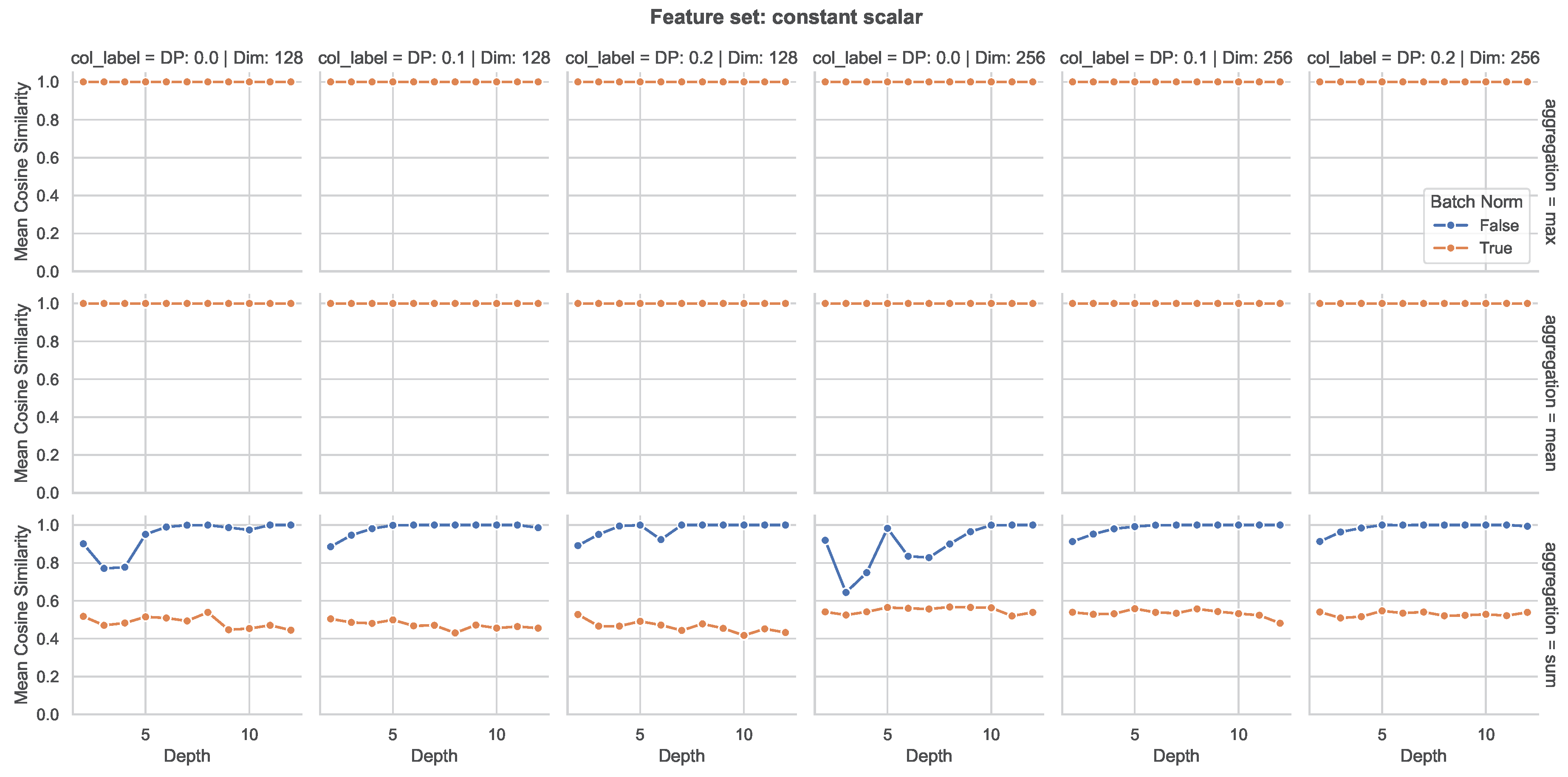
Figure A2.
Mean cosine similarity of node embeddings across network depths () using spectral moments as initial node features. Providing a fine-grained view of Figure 7, the layout contrasts aggregation operators, hidden dimensions (128 vs. 256), dropout rates (DP), and Batch Normalization (False vs. True). Higher similarity values at greater depths indicate severe embedding collapse due to oversmoothing. Due to spatial overlap in 2-hop ego-networks, spectral moments exhibit higher initial similarity, rendering representations particularly sensitive to overmixing without Batch Normalization.
Figure A2.
Mean cosine similarity of node embeddings across network depths () using spectral moments as initial node features. Providing a fine-grained view of Figure 7, the layout contrasts aggregation operators, hidden dimensions (128 vs. 256), dropout rates (DP), and Batch Normalization (False vs. True). Higher similarity values at greater depths indicate severe embedding collapse due to oversmoothing. Due to spatial overlap in 2-hop ego-networks, spectral moments exhibit higher initial similarity, rendering representations particularly sensitive to overmixing without Batch Normalization.
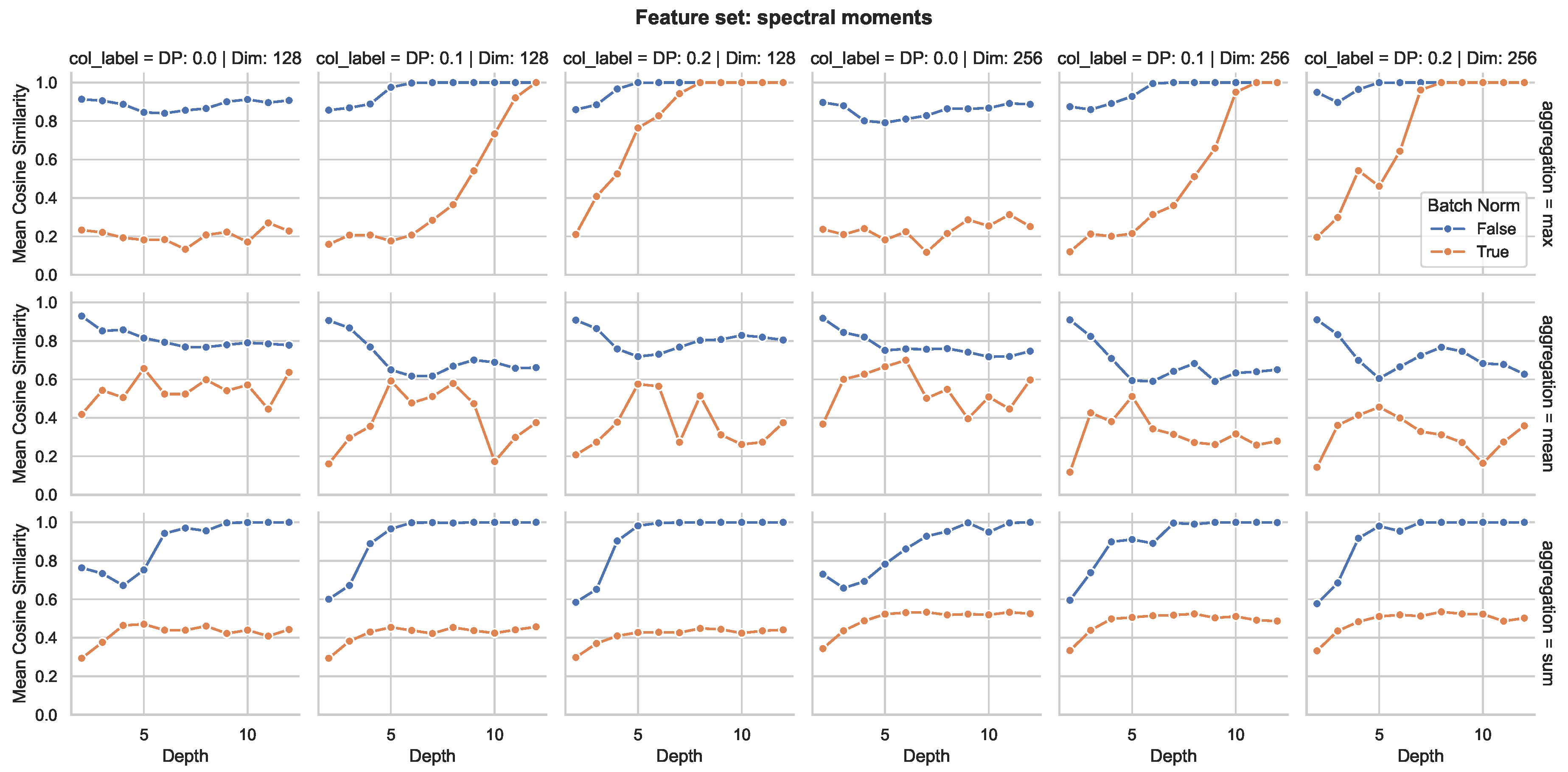
Figure A3.
Mean cosine similarity of node embeddings across network depths () using centralities and clustering coefficients as initial node features. Providing a fine-grained view of Figure 7, the layout contrasts aggregation operators, hidden dimensions (128 vs. 256), dropout rates (DP), and Batch Normalization (False vs. True). Higher similarity values at greater depths indicate severe embedding collapse due to oversmoothing. Across configurations, Batch Normalization acts as a primary stabilizer against feature alignment, whereas applying dropout significantly accelerates the onset of oversmoothing.
Figure A3.
Mean cosine similarity of node embeddings across network depths () using centralities and clustering coefficients as initial node features. Providing a fine-grained view of Figure 7, the layout contrasts aggregation operators, hidden dimensions (128 vs. 256), dropout rates (DP), and Batch Normalization (False vs. True). Higher similarity values at greater depths indicate severe embedding collapse due to oversmoothing. Across configurations, Batch Normalization acts as a primary stabilizer against feature alignment, whereas applying dropout significantly accelerates the onset of oversmoothing.
Appendix C. Supplementary Data on Subgraph Counting
Table A2.
Graphlet frequencies across test graphs.. Summary of exact graphlet frequencies across the evaluated test graphs for 3-node and 4-node graphlets.
Table A2.
Graphlet frequencies across test graphs.. Summary of exact graphlet frequencies across the evaluated test graphs for 3-node and 4-node graphlets.
| Network | G1 | G2 | G3 | G4 | G5 | G6 | G7 | G8 |
|---|---|---|---|---|---|---|---|---|
| BioSNAP | ||||||||
| 1 | 4,435,654 | 205,243 | 268,142,903 | 265,135,531 | 4,136,734 | 58,081,764 | 4,868,244 | 758,069 |
| 2 | 4,549,154 | 205,112 | 274,536,842 | 293,250,632 | 4,424,211 | 61,426,078 | 5,063,773 | 689,276 |
| 3 | 4,183,375 | 196,969 | 249,401,320 | 245,409,230 | 3,972,468 | 54,958,440 | 4,696,293 | 719,133 |
| 4 | 3,837,477 | 181,772 | 224,981,404 | 203,450,229 | 3,592,526 | 48,315,024 | 4,107,243 | 634,256 |
| 5 | 4,158,481 | 199,340 | 249,157,012 | 239,442,133 | 4,072,717 | 55,287,211 | 4,769,207 | 724,058 |
| 6 | 3,632,729 | 171,533 | 208,670,884 | 192,154,143 | 3,277,716 | 44,885,664 | 3,823,518 | 572,250 |
| 9 | 3,250,347 | 155,083 | 182,245,477 | 162,058,536 | 3,074,656 | 40,100,297 | 3,490,926 | 455,258 |
| 10 | 2,850,625 | 135,875 | 151,656,063 | 144,389,616 | 2,549,695 | 34,187,219 | 3,019,601 | 376,833 |
| 11 | 2,447,654 | 119,443 | 125,707,639 | 109,956,789 | 2,154,089 | 28,179,563 | 2,522,302 | 311,825 |
| 13 | 2,203,210 | 110,337 | 109,511,281 | 94,516,099 | 1,909,096 | 24,945,900 | 2,273,777 | 289,512 |
| 14 | 1,923,112 | 81,279 | 90,329,023 | 82,019,757 | 1,493,161 | 18,889,665 | 1,566,902 | 135,033 |
| 15 | 2,003,290 | 88,990 | 95,825,551 | 84,919,150 | 1,629,625 | 20,463,191 | 1,746,201 | 163,632 |
| 17 | 1,342,671 | 63,425 | 56,784,359 | 49,101,895 | 1,010,347 | 12,874,269 | 1,140,128 | 106,259 |
| 20 | 920,718 | 46,742 | 34,819,371 | 27,873,576 | 634,800 | 7,795,340 | 726,092 | 84,278 |
| 21 | 794,022 | 36,841 | 28,500,494 | 24,190,960 | 509,081 | 627,0871 | 548,340 | 45,212 |
| 22 | 705,214 | 37,107 | 24,351,908 | 20,426,610 | 467,211 | 5,939,218 | 570,387 | 54,335 |
| 23 | 355,272 | 18,214 | 9,861,073 | 8,112,061 | 197,373 | 2,354,552 | 225,910 | 18,813 |
| Cell Organelles | ||||||||
| Golgi | 908 | 65 | 2,138 | 1,930 | 17 | 348 | 34 | 22 |
| Vesicles | 6,323 | 275 | 33,141 | 23,562 | 271 | 4,721 | 435 | 66 |
| Cytoplasm | 676,190 | 103,059 | 17,415,133 | 13,823,226 | 157,167 | 7,714,747 | 1,507,684 | 1,155,823 |
| Nucleus | 1,509,862 | 413,929 | 53,257,395 | 53,257,395 | 40,796,340 | 398,964 | 29,685,746 | 3,768,939 |
Figure A4.
Heuristic detector workflow for 4-node graphlet enumeration. The circled orbit nodes serve as anchor points for the detector, activated when the model’s predicted probability exceeds 0.5 (). From these anchor nodes, the detector scans immediate neighborhood structures for “deal-breaker” edges (highlighted in red dashed lines) whose presence would violate structural induction, thereby filtering out non-induced subgraph instances.
Figure A4.
Heuristic detector workflow for 4-node graphlet enumeration. The circled orbit nodes serve as anchor points for the detector, activated when the model’s predicted probability exceeds 0.5 (). From these anchor nodes, the detector scans immediate neighborhood structures for “deal-breaker” edges (highlighted in red dashed lines) whose presence would violate structural induction, thereby filtering out non-induced subgraph instances.

Table A3.
Constant Scalar: Absolute Error of Graphlet Counts Across Test Graphs.
| Network | G1 | G2 | G3 | G4 | G5 | G6 | G7 | G8 |
|---|---|---|---|---|---|---|---|---|
| BioSNAP | ||||||||
| 1 | 0 | 0 | 0 | 0 | 6 | 0 | 0 | 0 |
| 2 | 0 | 1 | 0 | 0 | 0 | 0 | 2 | 2 |
| 3 | 0 | 0 | 0 | 0 | 0 | 0 | 0 | 1 |
| 4 | 0 | 0 | 0 | 0 | 1 | 0 | 0 | 4 |
| 5 | 0 | 0 | 0 | 0 | 0 | 0 | 0 | 19 |
| 6 | 0 | 0 | 0 | 0 | 0 | 0 | 0 | 18 |
| 9 | 0 | 0 | 0 | 0 | 0 | 0 | 2 | 3 |
| 10 | 0 | 0 | 0 | 0 | 0 | 0 | 0 | 3 |
| 11 | 0 | 0 | 0 | 0 | 0 | 0 | 0 | 0 |
| 13 | 0 | 0 | 0 | 0 | 0 | 0 | 0 | 0 |
| 14 | 0 | 0 | 0 | 0 | 3 | 0 | 0 | 0 |
| 15 | 0 | 0 | 0 | 0 | 1 | 0 | 0 | 0 |
| 17 | 0 | 1 | 0 | 0 | 0 | 0 | 0 | 1 |
| 20 | 0 | 1 | 0 | 0 | 0 | 0 | 0 | 7 |
| 21 | 0 | 5 | 0 | 0 | 1 | 0 | 0 | 16 |
| 22 | 0 | 1 | 0 | 0 | 0 | 0 | 1 | 6 |
| 23 | 0 | 0 | 0 | 0 | 0 | 0 | 0 | 6 |
| Cell Organelles | ||||||||
| Golgi | 0 | 4 | 0 | 0 | 13 | 0 | 20 | 7 |
| Vesicles | 0 | 3 | 0 | 1 | 14 | 0 | 11 | 25 |
| Cytoplasm | 0 | 1 | 0 | 0 | 7 | 0 | 4 | 14 |
| Nucleus | 0 | 6 | 0 | 0 | 3 | 0 | 1 | 9 |
Table A4.
Spectral Moments: Absolute Error of Graphlet Counts Across Test Graphs.
| Network | G1 | G2 | G3 | G4 | G5 | G6 | G7 | G8 |
|---|---|---|---|---|---|---|---|---|
| BioSNAP | ||||||||
| 1 | 0 | 0 | 0 | 0 | 6 | 0 | 1 | 0 |
| 2 | 0 | 0 | 0 | 0 | 0 | 0 | 1 | 0 |
| 3 | 0 | 0 | 0 | 0 | 0 | 0 | 0 | 0 |
| 4 | 0 | 0 | 0 | 0 | 1 | 0 | 0 | 0 |
| 5 | 0 | 0 | 0 | 0 | 2 | 0 | 0 | 0 |
| 6 | 0 | 0 | 0 | 0 | 2 | 0 | 0 | 0 |
| 9 | 0 | 0 | 0 | 0 | 0 | 0 | 1 | 0 |
| 10 | 0 | 0 | 0 | 0 | 0 | 0 | 1 | 0 |
| 11 | 0 | 0 | 0 | 0 | 0 | 0 | 1 | 0 |
| 13 | 0 | 0 | 0 | 0 | 2 | 0 | 0 | 0 |
| 14 | 0 | 0 | 0 | 0 | 3 | 0 | 0 | 0 |
| 15 | 0 | 0 | 0 | 0 | 1 | 0 | 0 | 1 |
| 17 | 0 | 0 | 0 | 0 | 0 | 0 | 0 | 1 |
| 20 | 0 | 0 | 0 | 0 | 0 | 0 | 0 | 0 |
| 21 | 0 | 0 | 0 | 0 | 1 | 0 | 0 | 0 |
| 22 | 0 | 0 | 0 | 0 | 0 | 0 | 0 | 0 |
| 23 | 0 | 0 | 0 | 0 | 0 | 0 | 0 | 0 |
| Cell Organelles | ||||||||
| Golgi | 0 | 1 | 0 | 0 | 12 | 1 | 2 | 0 |
| Vesicles | 0 | 3 | 0 | 0 | 14 | 0 | 5 | 3 |
| Cytoplasm | 0 | 0 | 0 | 0 | 8 | 0 | 1 | 8 |
| Nucleus | 0 | 0 | 0 | 0 | 5 | 0 | 0 | 1 |
Table A5.
Centralities and Clustering Coefficient: Absolute Error of Graphlet Counts Across Test Graphs.
Table A5.
Centralities and Clustering Coefficient: Absolute Error of Graphlet Counts Across Test Graphs.
| Network | G1 | G2 | G3 | G4 | G5 | G6 | G7 | G8 |
|---|---|---|---|---|---|---|---|---|
| BioSNAP | ||||||||
| 1 | 0 | 0 | 0 | 0 | 6 | 0 | 0 | 0 |
| 2 | 0 | 0 | 0 | 0 | 0 | 0 | 1 | 0 |
| 3 | 0 | 0 | 0 | 0 | 3 | 0 | 0 | 0 |
| 4 | 0 | 0 | 0 | 0 | 1 | 0 | 0 | 0 |
| 5 | 0 | 0 | 0 | 0 | 0 | 0 | 0 | 0 |
| 6 | 0 | 0 | 0 | 0 | 1 | 0 | 0 | 0 |
| 9 | 0 | 0 | 0 | 0 | 0 | 0 | 0 | 0 |
| 10 | 0 | 0 | 0 | 0 | 0 | 0 | 0 | 0 |
| 11 | 0 | 0 | 0 | 0 | 0 | 0 | 0 | 0 |
| 13 | 0 | 0 | 0 | 0 | 2 | 0 | 0 | 0 |
| 14 | 0 | 0 | 0 | 1 | 3 | 0 | 0 | 0 |
| 15 | 0 | 0 | 0 | 0 | 1 | 0 | 0 | 0 |
| 17 | 0 | 0 | 0 | 0 | 0 | 0 | 0 | 10 |
| 20 | 0 | 0 | 0 | 0 | 1 | 0 | 0 | 0 |
| 21 | 0 | 0 | 0 | 0 | 0 | 0 | 0 | 0 |
| 22 | 0 | 0 | 0 | 0 | 0 | 0 | 0 | 0 |
| 23 | 0 | 0 | 0 | 0 | 0 | 0 | 0 | 0 |
| Cell Organelles | ||||||||
| Golgi | 0 | 0 | 0 | 4 | 10 | 0 | 1 | 1 |
| Vesicles | 0 | 0 | 0 | 10 | 24 | 0 | 4 | 6 |
| Cytoplasm | 0 | 0 | 0 | 1 | 4 | 0 | 0 | 3 |
| Nucleus | 0 | 0 | 0 | 1 | 4 | 0 | 6 | 1 |
References
- Agrawal, M.; Zitnik, M.; Leskovec, J. Large-scale analysis of disease pathways in the human interactome. Pac. Symp. Biocomput. 2018, 23, 111–122. [Google Scholar] [CrossRef]
- Aguilar, C.O. An Introduction to Algebraic Graph Theory; State University of New York: Geneseo, NY, USA, 2021; p. 149. [Google Scholar]
- Albert, R.; Barabási, A.-L. Statistical mechanics of complex networks. Rev. Mod. Phys. 2002, 74, 47–97. [Google Scholar] [CrossRef]
- Alon, U. Network motifs: theory and experimental approaches. Nat. Rev. Genet. 2007, 8, 450–461. [Google Scholar] [CrossRef] [PubMed]
- Alon, U.; Yahav, E. On the bottleneck of graph neural networks and its practical implications. arXiv 2020, arXiv:2006.05205. [Google Scholar]
- Arnaiz-Rodríguez, A.; Errica, F. Oversmoothing, “Oversquashing”, Heterophily, Long-Range, and more: Demystifying Common Beliefs in Graph Machine Learning. In Proceedings of the 14th International Conference on Learning Representations (ICLR 2026), Rio de Janeiro, Brazil, 23–27 April 2026; Volume 2026, pp. 62884–62910. [Google Scholar]
- Bainson, A.B.; Hermanns, J.; Petsinis, P.; Aavad, N.; Larsen, C.D.; Swayne, T.; Boyarski, A.; Mottin, D.; Bronstein, A.M.; Karras, P. Spectral Subgraph Localization. In Proceedings of the Second Learning on Graphs Conference, Virtual, 27–30 November 2023; Villar, S., Chamberlain, B., Eds.; PMLR, 2024; Volume 231, pp. 7:1–7:11. [Google Scholar]
- Barabási, A.-L. Network Science; Cambridge University Press: Cambridge, UK, 2016. [Google Scholar]
- Butler, S.K. Eigenvalues and Structures of Graphs. Ph.D. Thesis, University of California, San Diego, CA, USA, 2008. [Google Scholar]
- Cai, C.; Wang, Y. A note on over-smoothing for graph neural networks. arXiv 2020, arXiv:2006.13318. [Google Scholar]
- Chen, X.; Li, Y.; Wang, P.; Lui, J.C.S. A general framework for estimating graphlet statistics via random walk. Proc. VLDB Endow. 2016, 10, 253–264. [Google Scholar] [CrossRef]
- Chen, D.; Lin, Y.; Li, W.; Li, P.; Zhou, J.; Sun, X. Measuring and Relieving the Over-Smoothing Problem for Graph Neural Networks from the Topological View. In Proceedings of the 34th AAAI Conference on Artificial Intelligence (AAAI 2020), New York, NY, USA, 7–12 February 2020; Volume 34, pp. 3438–3445. [Google Scholar]
- Chen, Z.; Chen, L.; Villar, S.; Bruna, J. Can graph neural networks count substructures? In Proceedings of the 34th International Conference on Neural Information Processing Systems (NeurIPS 2020), Vancouver, BC, Canada, 6–12 December 2020; Curran Associates Inc.: Red Hook, NY, USA, 2020; pp. 10383–10395. [Google Scholar]
- Ciano, G.; Rossi, A.; Bianchini, M.; Scarselli, F. On inductive–transductive learning with graph neural networks. IEEE Trans. Pattern Anal. Mach. Intell. 2022, 44, 758–769. [Google Scholar] [CrossRef] [PubMed]
- Ciriello, G.; Guerra, C. A review on models and algorithms for motif discovery in protein–protein interaction networks. Brief. Funct. Genom. Proteom. 2008, 7, 147–156. [Google Scholar] [CrossRef] [PubMed]
- Cohen-Steiner, D.; Kong, W.; Sohler, C.; Valiant, G. Approximating the spectrum of a graph. In Proceedings of the 24th ACM SIGKDD International Conference on Knowledge Discovery & Data Mining (KDD ’18), London, UK, 19–23 August 2018; Association for Computing Machinery: New York, NY, USA, 2018; pp. 1263–1271. [Google Scholar]
- Epping, B.; René, A.; Helias, M.; Schaub, M.T. Graph neural networks do not always oversmooth. In Proceedings of the 38th Conference on Neural Information Processing Systems (NeurIPS 2024), Vancouver, BC, Canada, 10–15 December 2024; Volume 37, pp. 48164–48188. [Google Scholar]
- Gong, C.-H.; Wang, L.; Shi, C.; Zhou, D.; Liu, M.; Zhang, X.; Zhao, J.; et al. A survey on learning from graphs with heterophily: Recent advances and future directions. Front. Comput. Sci. 2026, 20, 2002314. [Google Scholar] [CrossRef]
- Gosak, M.; Markovič, R.; Dolenšek, J.; Slak Rupnik, M.; Marhl, M.; Stožer, A.; Perc, M. Network science of biological systems at different scales: A review. Phys. Life Rev. 2018, 24, 118–135. [Google Scholar] [CrossRef] [PubMed]
- Hamilton, W.L. Graph Representation Learning; Synthesis Lectures on Artificial Intelligence and Machine Learning; Morgan & Claypool Publishers: San Rafael, CA, USA, 2020; Volume 14, p. 159. [Google Scholar]
- Hamilton, W.; Ying, Z.; Leskovec, J. Inductive representation learning on large graphs. In Proceedings of the 31st International Conference on Neural Information Processing Systems (NIPS 2017); Long Beach, CA, USA, 4–9 December 2017, Guyon, I., Luxburg, U.V., Bengio, S., Wallach, H., Fergus, R., Vishwanathan, S., Garnett, R., Eds.; Curran Associates Inc.: Red Hook, NY, USA, 2017; pp. 1025–1034. [Google Scholar]
- Hartwell, L.H.; Hopfield, J.J.; Leibler, S.; Murray, A.W. From molecular to modular cell biology. Nature 1999, 402, C47–C52. [Google Scholar] [CrossRef] [PubMed]
- Hočevar, T.; Demšar, J. A combinatorial approach to graphlet counting. Bioinformatics 2014, 30, 559–565. [Google Scholar] [CrossRef] [PubMed]
- Ioffe, S.; Szegedy, C. Batch normalization: Accelerating deep network training by reducing internal covariate shift. In Proceedings of the 32nd International Conference on Machine Learning (ICML 2015); Lille, France, 6–11 July 2015, Bach, F., Blei, D., Eds.; PMLR, 2015; Volume 37, pp. 448–456. [Google Scholar]
- Jin, S.; Zafarani, R. The spectral zoo of networks: Embedding and visualizing networks with spectral moments. In Proceedings of the 26th ACM SIGKDD International Conference on Knowledge Discovery & Data Mining (KDD ’20), CA, USA, 23–27 August 2020; Association for Computing Machinery: New York, NY, USA, 2020; pp. 1426–1434. [Google Scholar]
- Jin, S.; Tian, H.; Li, J.; Zafarani, R. A spectral representation of networks: The path of subgraphs. In Proceedings of the 28th ACM SIGKDD Conference on Knowledge Discovery and Data Mining (KDD ’22), Washington, DC, USA, 14–18 August 2022; Association for Computing Machinery: New York, NY, USA, 2022; pp. 698–708. [Google Scholar]
- Joyce, K.E.; Hayasaka, S.; Laurienti, P.J. The human functional brain network demonstrates structural and dynamical resilience to targeted attack. PLoS Comput. Biol. 2013, 9, e1002885. [Google Scholar] [CrossRef] [PubMed]
- Khemani, B.; Patil, S.; Kotecha, K.; Tanwar, S. A review of graph neural networks: concepts, architectures, techniques, challenges, datasets, applications, and future directions. J. Big Data 2024, 11, 18. [Google Scholar] [CrossRef]
- Lan, Z.; Yu, L.; Yuan, L.; Wu, Z.; Niu, Q.; Ma, F. Sub-gmn: The neural subgraph matching network model. In Proceedings of the 2023 16th International Congress on Image and Signal Processing, BioMedical Engineering and Informatics (CISP-BMEI), Ta Episcopi, China, 28–30 October 2023; IEEE: Piscataway, NJ, USA, 2023; pp. 1–7. [Google Scholar]
- Lipton, Z.C.; Elkan, C.; Naryanaswamy, B. Optimal thresholding of classifiers to maximize F1 measure. In Machine Learning and Knowledge Discovery in Databases, Proceedings of the European Conference on Machine Learning and Knowledge Discovery in Databases (ECML PKDD 2014); Nancy, France, 15–19 September 2014, Calders, T., Esposito, F., Hüllermeier, E., Meo, R., Eds.; Springer: Berlin/Heidelberg, Germany, 2014; pp. 225–239. [Google Scholar]
- Liu, C.; Ma, Y.; Zhao, J.; Nussinov, R.; Zhang, Y.-C.; Cheng, F.; Zhang, Z.-K. Computational network biology: Data, models, and applications. Phys. Rep. 2020, 846, 1–66. [Google Scholar] [CrossRef]
- Liu, M.; Gao, H.; Ji, S. Towards deeper graph neural networks. In Proceedings of the 26th ACM SIGKDD International Conference on Knowledge Discovery & Data Mining, Virtual Event, CA, USA, 6–10 July 2020; pp. 338–348. [Google Scholar]
- Luck, K.; Kim, D.-K.; Lambourne, L.; Spirohn, K.; Begg, B.E.; Bian, W.; Brignall, R.; Cafarelli, T.M.; Campos-Laborie, F.J.; Charloteaux, B.; et al. A reference map of the human binary protein interactome. Nature 2020, 580, 402–408. [Google Scholar] [CrossRef] [PubMed]
- Maharaj, S.K. Graphlet Analysis Of Networks. Ph.D. Thesis, University of California, Irvine, CA, USA, 2018. [Google Scholar]
- Maslov, S.; Sneppen, K. Specificity and stability in topology of protein networks. Science 2002, 296, 910–913. [Google Scholar] [CrossRef] [PubMed]
- Melckenbeeck, I.; Audenaert, P.; Colle, D.; Pickavet, M. Efficiently counting all orbits of graphlets of any order in a graph using autogenerated equations. Bioinformatics 2018, 34, 1372–1380. [Google Scholar] [CrossRef] [PubMed]
- Menche, J.; Sharma, A.; Kitsak, M.; Ghiassian, S.D.; Vidal, M.; Loscalzo, J.; Barabási, A.-L. Uncovering disease-disease relationships through the incomplete interactome. Science 2015, 347, 1257601. [Google Scholar] [CrossRef] [PubMed]
- Milo, R.; Shen-Orr, S.; Itzkovitz, S.; Kashtan, N.; Chklovskii, D.; Alon, U. Network motifs: Simple building blocks of complex networks. Science 2002, 298, 824–827. [Google Scholar] [CrossRef] [PubMed]
- Mironov, M.; Prokhorenkova, L. Revisiting graph homophily measures. arXiv 2024, arXiv:2412.09663. [Google Scholar]
- Moayed, H.; Mansoori, E.G.; Moosavi, M.R. An efficient pruning method for subgraph matching in large-scale graphs. J. Supercomput. 2023, 79, 10511–10532. [Google Scholar] [CrossRef]
- Moreno, D.; Neller, J.; Kestler, H.A.; Kraus, J.; Dünkler, A.; Johnsson, N. A fluorescent reporter for mapping cellular protein-protein interactions in time and space. Mol. Syst. Biol. 2013, 9, 647. [Google Scholar] [CrossRef] [PubMed]
- Patra, S.; Mohapatra, A. Review of tools and algorithms for network motif discovery in biological networks. IET Syst. Biol. 2020, 14, 171–189. [Google Scholar] [CrossRef] [PubMed]
- Pržulj, N. Biological network comparison using graphlet degree distribution. Bioinformatics 2007, 23, e177–e183. [Google Scholar] [CrossRef] [PubMed]
- Read, J.; Pfahringer, B.; Holmes, G.; Frank, E. Classifier chains for multi-label classification. Mach. Learn. 2011, 85, 333–359. [Google Scholar] [CrossRef]
- Ribeiro, P.; Paredes, P.; Silva, M.E.; Aparicio, D.; Silva, F. A survey on subgraph counting: Concepts, algorithms, and applications to network motifs and graphlets. ACM Comput. Surv. 2021, 54, 1–36. [Google Scholar]
- Rusch, T.K.; Bronstein, M.M.; Mishra, S. A survey on oversmoothing in graph neural networks. arXiv 2023, arXiv:2303.10993. [Google Scholar]
- Shen-Orr, S.S.; Milo, R.; Mangan, S.; Alon, U. Network motifs in the transcriptional regulation network of Escherichia coli. Nat. Genet. 2002, 31, 64–68. [Google Scholar] [CrossRef] [PubMed]
- Stolnicu, A.; Ikonomi, N.; Eckhardt-Bellmann, P.; Kraus, J.M.; Kestler, H.A. Robust signalling entropy estimation for biological process characterisation. Brief. Bioinform. 2025, 26, bbaf269. [Google Scholar] [CrossRef] [PubMed]
- Strogatz, S.H. Exploring complex networks. Nature 2001, 410, 268–276. [Google Scholar] [CrossRef] [PubMed]
- Thul, P.J.; Åkesson, L.; Wiking, M.; Mahdessian, D.; Geladaki, A.; Ait Blal, H.; Alber, L.; Alm, T.; Asp, J.P.; Amstutz, C.; et al. A subcellular map of the human proteome. Science 2017, 356, eaal3321. [Google Scholar] [CrossRef] [PubMed]
- Van Dam, E.R.; Haemers, W.H. Which graphs are determined by their spectrum? Linear Algebra Appl. 2003, 373, 241–272. [Google Scholar] [CrossRef]
- Van den Heuvel, M.P.; Bullmore, E.T.; Sporns, O. Comparative connectomics. Trends Cogn. Sci. 2016, 20, 345–361. [Google Scholar] [CrossRef] [PubMed]
- Vazquez, A.; Dobrin, R.; Sergi, D.; Eckmann, J.-P.; Oltvai, Z.N.; Barabási, A.-L. The topological relationship between the large-scale attributes and local interaction patterns of complex networks. Proc. Natl. Acad. Sci. USA 2004, 101, 17940–17945. [Google Scholar] [CrossRef] [PubMed]
- Wernicke, S.; Rasche, F. FANMOD: A tool for fast network motif detection. Bioinformatics 2006, 22, 1152–1153. [Google Scholar] [CrossRef] [PubMed]
- Wilson, R.C.; Zhu, P. A study of graph spectra for comparing graphs and trees. Pattern Recognit. 2008, 41, 2833–2841. [Google Scholar] [CrossRef]
- Windels, S.F.L.; Malod-Dognin, N.; Pržulj, N. Graphlet Laplacians: Graphlet-based neighbourhoods highlight topology-function and topology-disease relationships. bioRxiv 2018. [Google Scholar] [CrossRef]
- Wong, E.; Baur, B.; Quader, S.; Huang, C.H. Biological network motif detection: Principles and practice. Brief. Bioinform. 2012, 13, 202–215. [Google Scholar] [CrossRef] [PubMed]
- Xu, K.; Hu, W.; Leskovec, J.; Jegelka, S. How powerful are graph neural networks? arXiv 2018, arXiv:1810.00826. [Google Scholar]
- Yan, Z.; Zhou, J.; Gao, L.; Tang, Z.; Zhang, M. An efficient subgraph gnn with provable substructure counting power. In Proceedings of the 30th ACM SIGKDD Conference on Knowledge Discovery and Data Mining, Barcelona, Spain, 25–29 August 2024; pp. 3702–3713. [Google Scholar]
- Yaveroğlu, Ö.N.; Milenković, T.; Pržulj, N. Proper evaluation of alignment-free network comparison methods. Bioinformatics 2015, 31, 2697–2704. [Google Scholar] [CrossRef] [PubMed]
- Zitnik, M.; Sosič, R.; Maheshwari, S.; Leskovec, J. BioSNAP Datasets. Available online: https://snap.stanford.edu/biodata.
- Zitnik, M.; Li, M.M.; Wells, A.; Glass, K.; Morselli Gysi, D.; Krishnan, A.; Murali, T.M.; Radivojac, P.; Roy, S.; Baudot, A.; et al. Current and future directions in network biology. Bioinform. Adv. 2024, 4, vbae099. [Google Scholar] [CrossRef] [PubMed]
- Zhao, T.; Dong, N.T.; Hanjalic, A.; Khosla, M. Multi-label node classification on graph-structured data. arXiv 2023, arXiv:2304.10398. [Google Scholar]
Figure 1.
Non-isomorphic connected graphlets of size up to five nodes. Different colors represent distinct automorphism orbits, reflecting structural node roles. (Source: adapted from [23])
Figure 1.
Non-isomorphic connected graphlets of size up to five nodes. Different colors represent distinct automorphism orbits, reflecting structural node roles. (Source: adapted from [23])
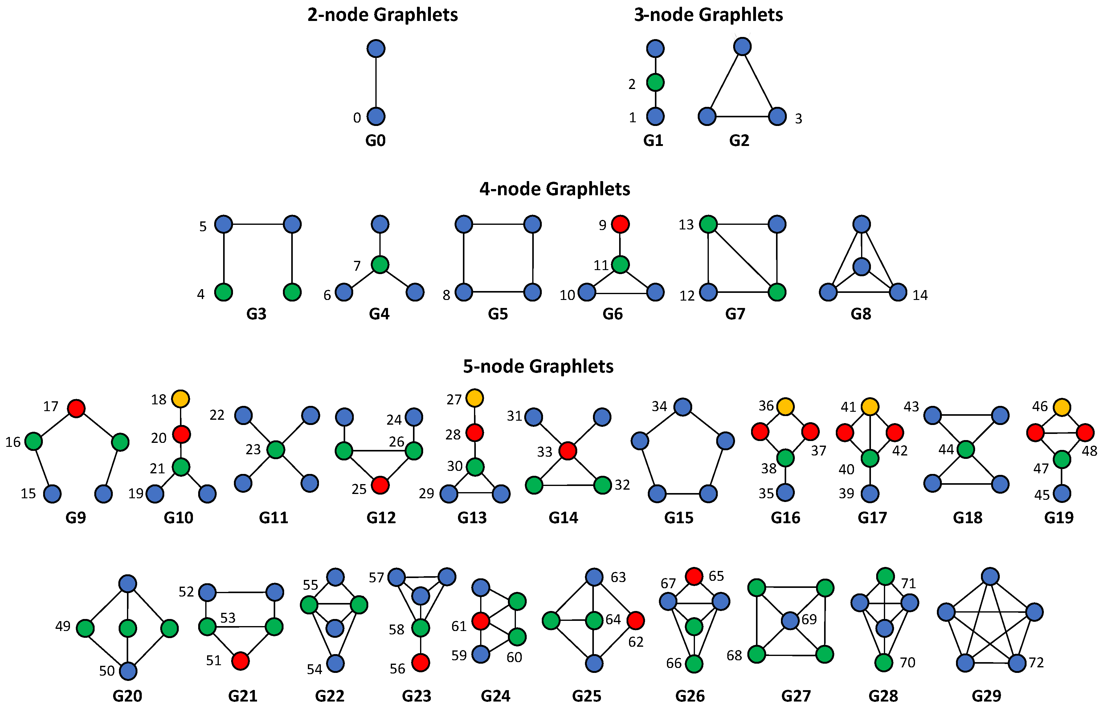
Figure 2.
Message passing mechanism in GNNs. The target node (A) collects information from its neighbors, who may first process their own neighborhood features before aggregation. The aggregated message is then used to update the embedding of node A. (Source: adapted from [20]).
Figure 2.
Message passing mechanism in GNNs. The target node (A) collects information from its neighbors, who may first process their own neighborhood features before aggregation. The aggregated message is then used to update the embedding of node A. (Source: adapted from [20]).
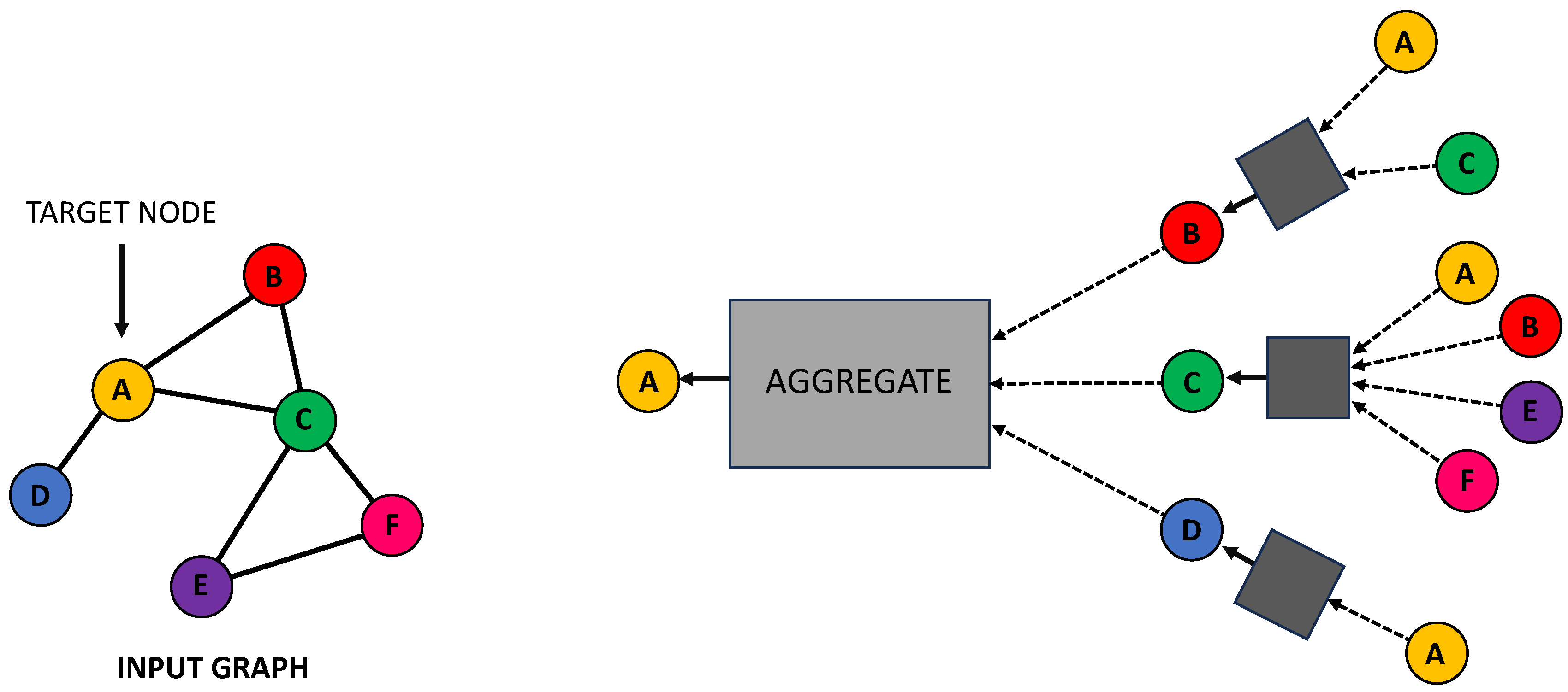
Figure 3.
Examples of graph structures that mean and max aggregators fail to distinguish. v and v’ get the same embedding even though their corresponding structures differ. Here, node colors denote different node features. (Source: adapted from [58]).
Figure 3.
Examples of graph structures that mean and max aggregators fail to distinguish. v and v’ get the same embedding even though their corresponding structures differ. Here, node colors denote different node features. (Source: adapted from [58]).
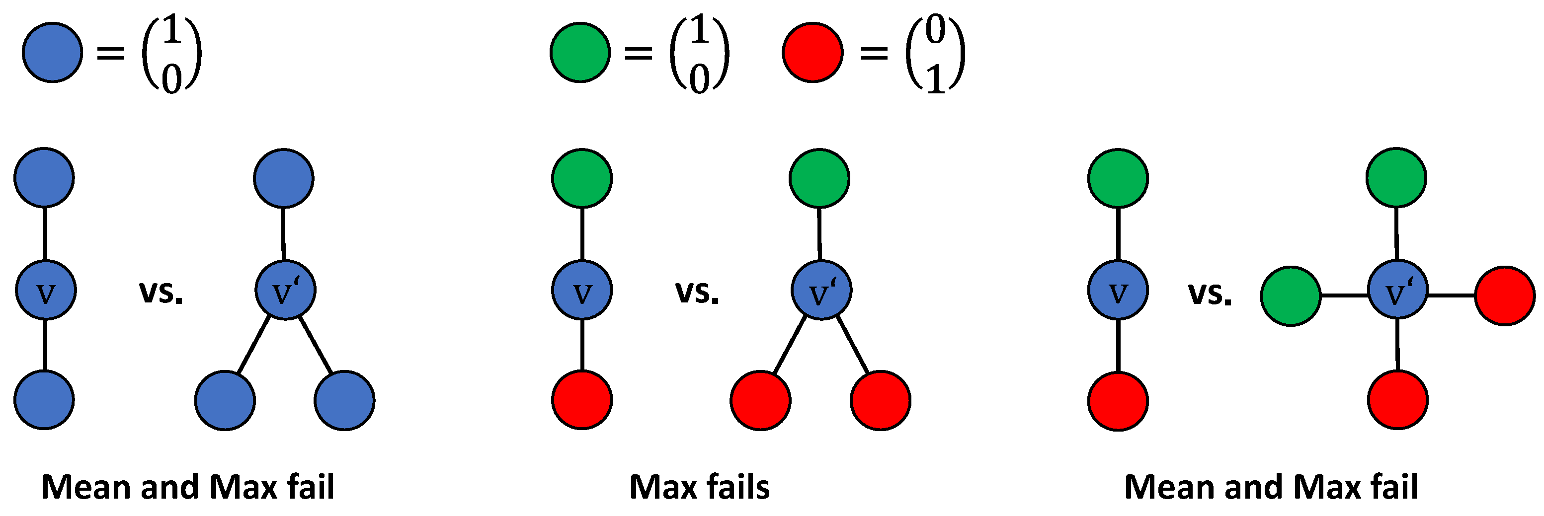
Figure 4.
Normalized label frequency of nodes participating in graphlets 1 to 29. Ground-truth labels are obtained by binarizing ORCA-derived graphlet degree vectors.
Figure 4.
Normalized label frequency of nodes participating in graphlets 1 to 29. Ground-truth labels are obtained by binarizing ORCA-derived graphlet degree vectors.
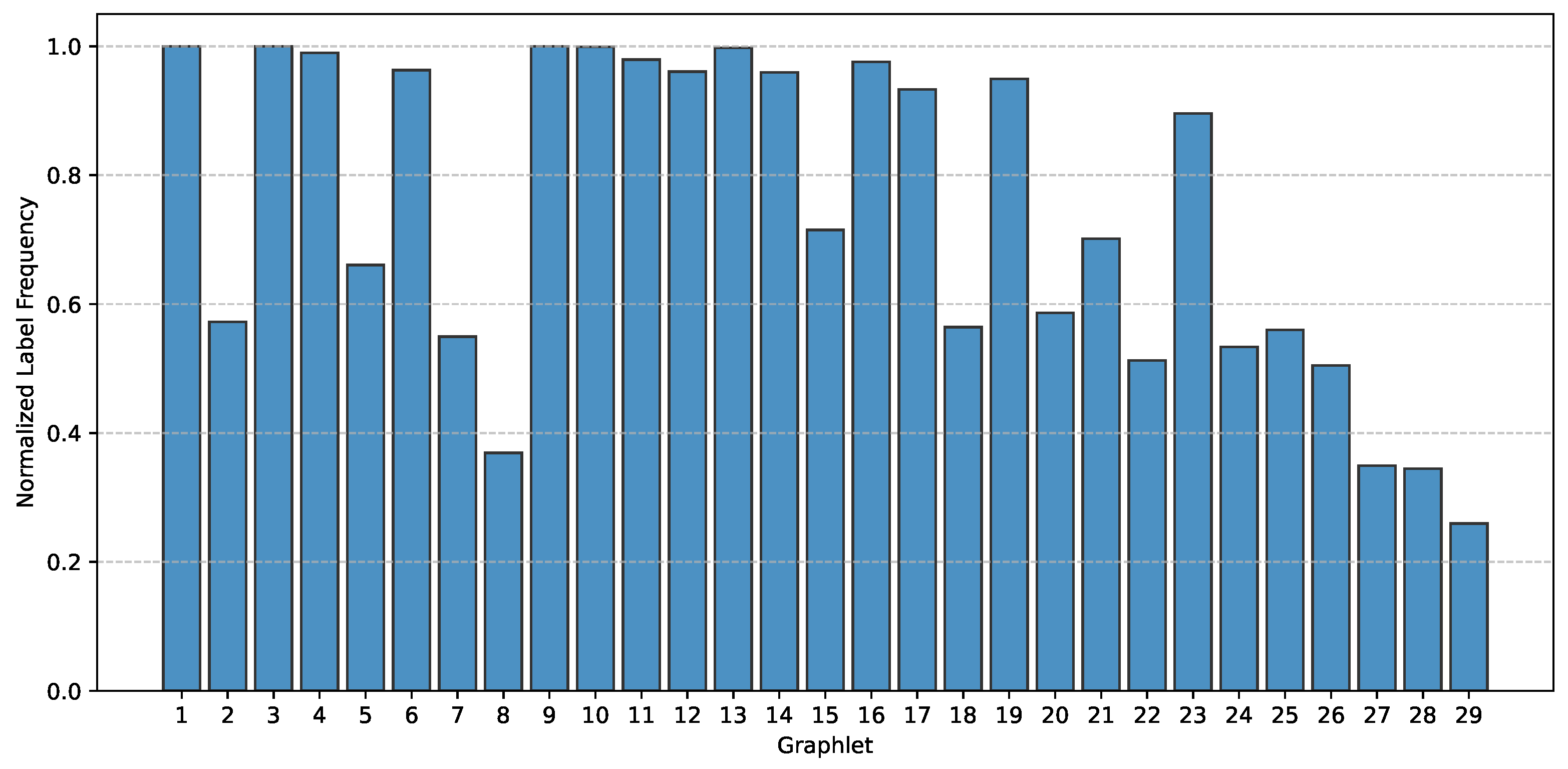
Figure 5.
Effect of network depth and aggregation function across different feature sets.
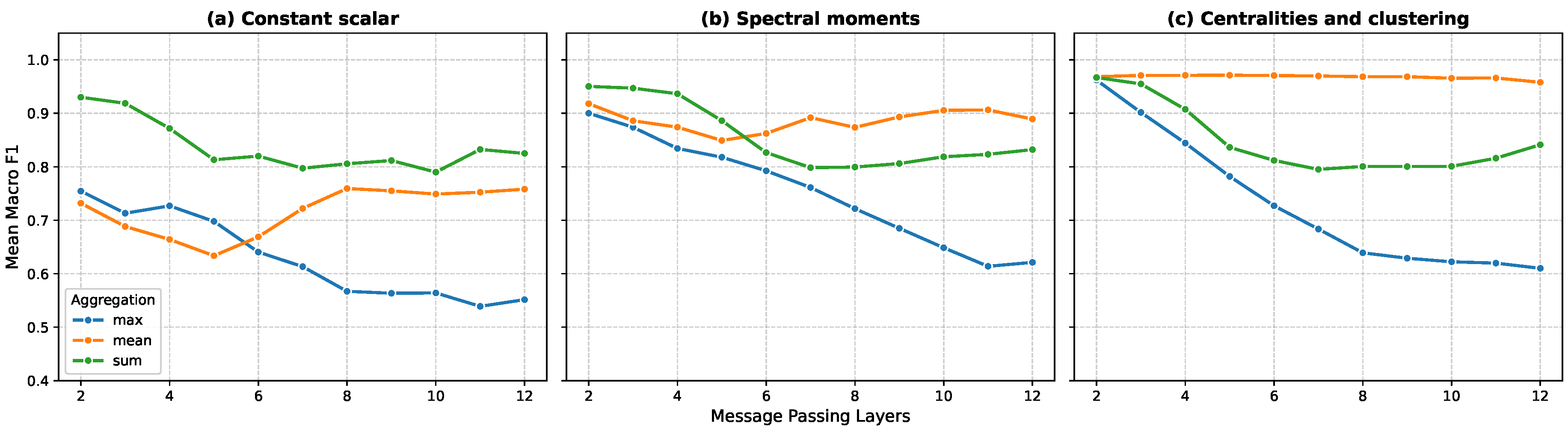
Figure 7.
Mean cosine similarity of node embeddings across network depths (). Subplots (a), (b), and (c) contrast different input feature sets (constant scalar, spectral moments, and centralities with clustering coefficients), illustrating the impact of Batch Normalization on layer-wise embedding separability.
Figure 7.
Mean cosine similarity of node embeddings across network depths (). Subplots (a), (b), and (c) contrast different input feature sets (constant scalar, spectral moments, and centralities with clustering coefficients), illustrating the impact of Batch Normalization on layer-wise embedding separability.
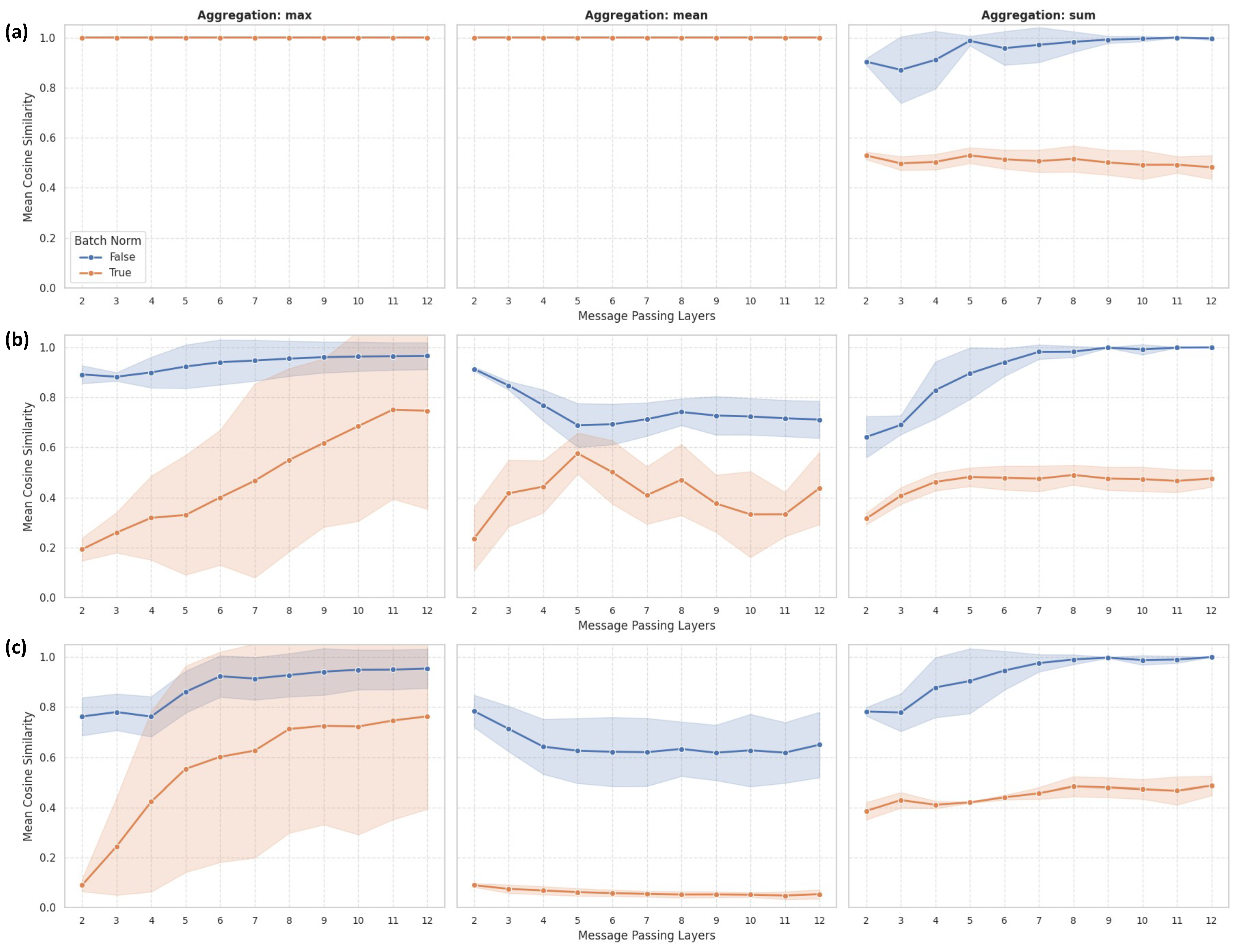
Figure 8.
Mean graphlet precisions across 5 splits. The results highlight feature- and aggregation-dependent performance variations, reflecting both structural failure cases (e.g., in cycles and clique-graphs) and class-imbalance-driven underperformance in underrepresented graphlet classes.
Figure 8.
Mean graphlet precisions across 5 splits. The results highlight feature- and aggregation-dependent performance variations, reflecting both structural failure cases (e.g., in cycles and clique-graphs) and class-imbalance-driven underperformance in underrepresented graphlet classes.
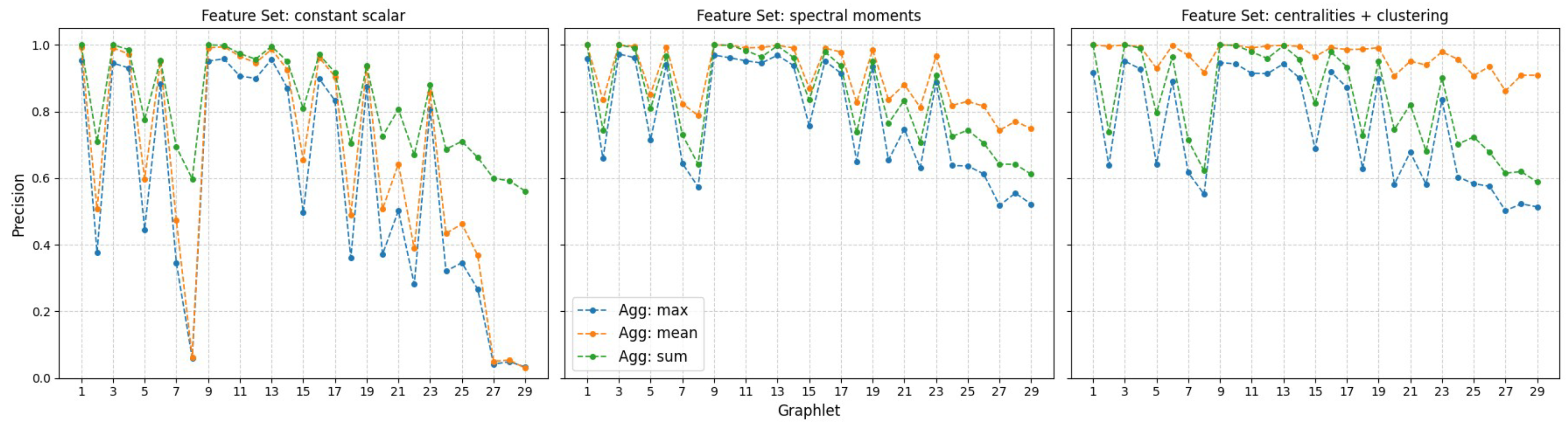
Figure 9.
Higher-order label homophily per graphlet class across k-hop neighborhoods (), computed via Equation 3. The values reflect the ratio of identically labeled neighbors at distance k.
Figure 9.
Higher-order label homophily per graphlet class across k-hop neighborhoods (), computed via Equation 3. The values reflect the ratio of identically labeled neighbors at distance k.
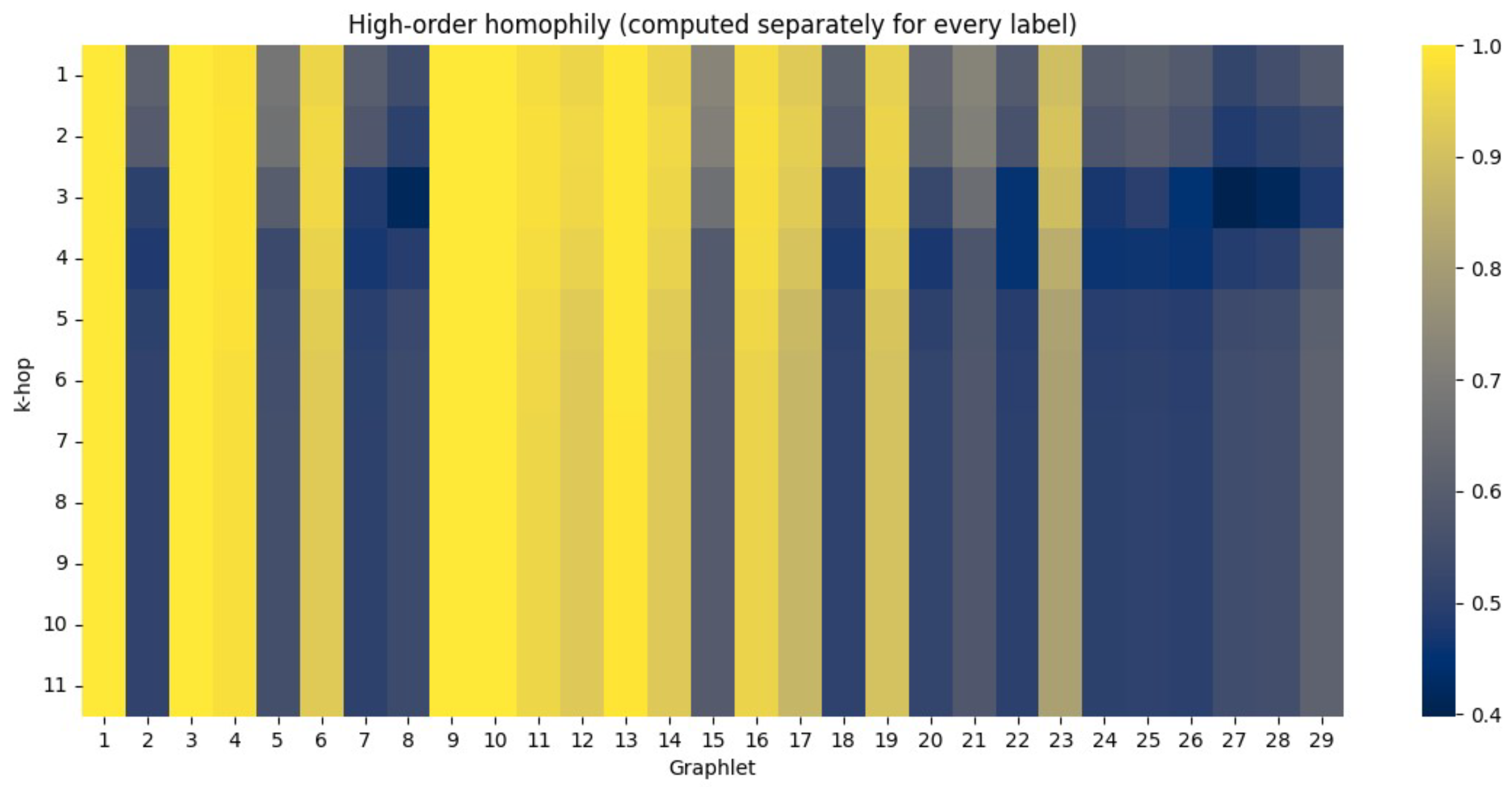
Figure 10.
Mean macro F1 across different feature sets. Each subpanel reports the results of a full-grid search over architectural design dimensions: depth, aggregation function, dropout rate, batch normalization, and hidden dimension size. Error bars represent standard deviations across all configurations sharing the same design choice. (a): constant scalar feature set, (b): spectral moments, (c): centralities and clustering coefficient
Figure 10.
Mean macro F1 across different feature sets. Each subpanel reports the results of a full-grid search over architectural design dimensions: depth, aggregation function, dropout rate, batch normalization, and hidden dimension size. Error bars represent standard deviations across all configurations sharing the same design choice. (a): constant scalar feature set, (b): spectral moments, (c): centralities and clustering coefficient
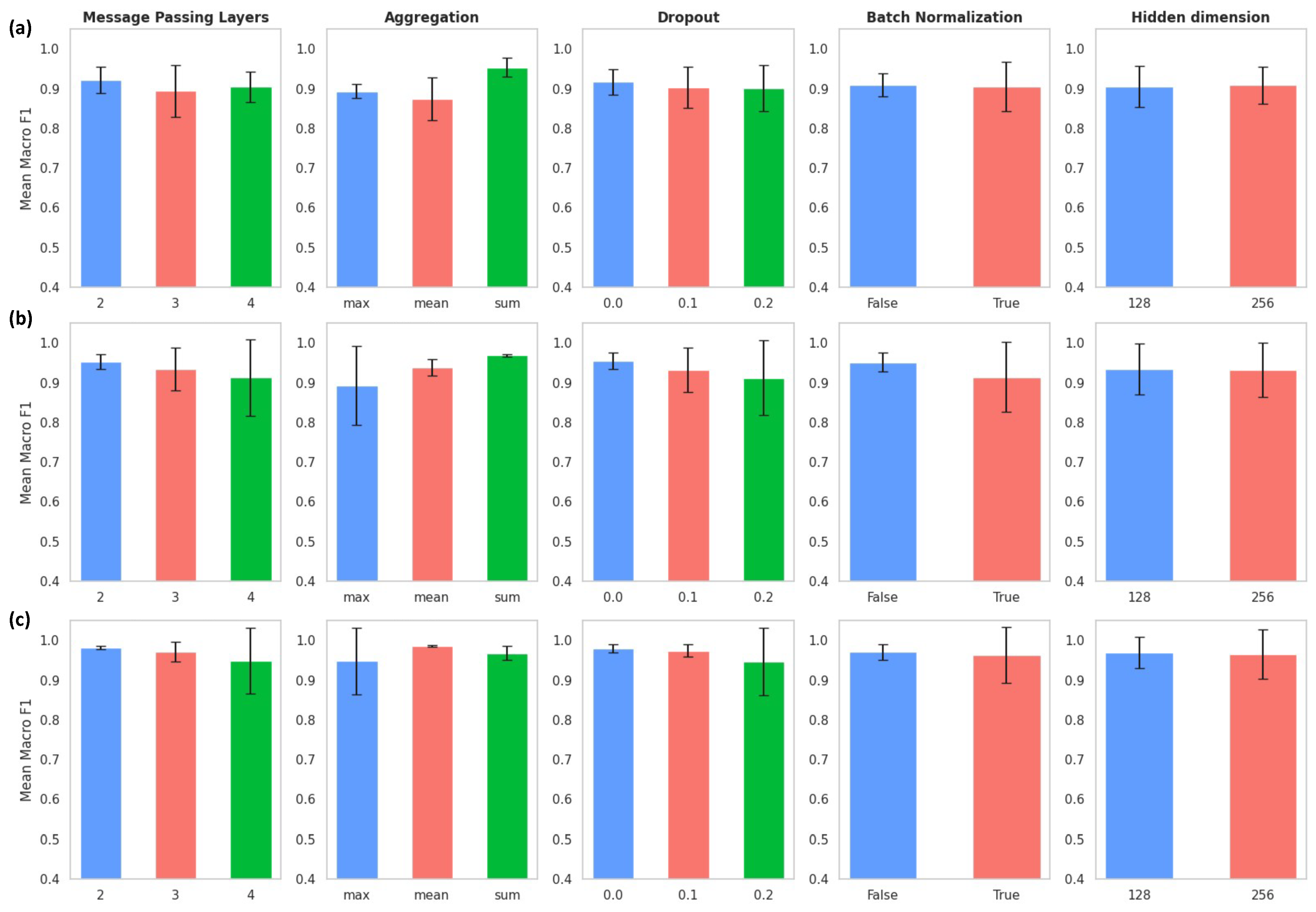
Figure 11.
Mean graphlet precisions across 5 splits in the inductive setting. Compared to the transductive setup, the larger and more diverse training data yields smoother precision profiles, though Constant Scalar features still exhibit aggregation-dependent structural failure cases.
Figure 11.
Mean graphlet precisions across 5 splits in the inductive setting. Compared to the transductive setup, the larger and more diverse training data yields smoother precision profiles, though Constant Scalar features still exhibit aggregation-dependent structural failure cases.
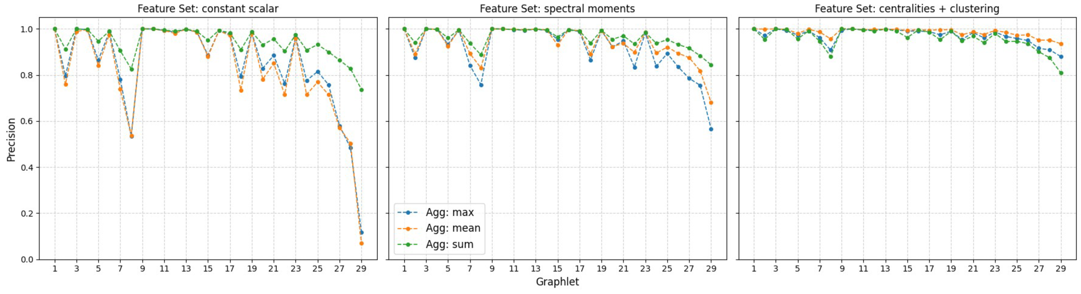
Table 1.
Condensed configuration space for the inductive GNN setting.
| Number of Layers | Aggregation | Batch norm. | Dropout | Hidden dim. |
|---|---|---|---|---|
| 2, 3, 4 | max, mean, sum | False, True | 0.0, 0.1, 0.2 | 128, 256 |
Table 2.
Macro-F1 evaluation per feature set for inductive node classification. Comparison of feature sets across test graphs with associated homophily and Jensen-Shannon divergence (JSD).
Table 2.
Macro-F1 evaluation per feature set for inductive node classification. Comparison of feature sets across test graphs with associated homophily and Jensen-Shannon divergence (JSD).
| Network | Homophily | JSD | Macro F1 | |||
|---|---|---|---|---|---|---|
| Constant | Spectral | Node | ||||
| BioSNAP | ||||||
| 1 | 3,480 | 0.9756 | 0.9751 | 0.9771 | 0.9771 | |
| 2 | 3,312 | 0.9787 | 0.9780 | 0.9794 | 0.9794 | |
| 3 | 3,284 | 0.9765 | 0.9764 | 0.9779 | 0.9779 | |
| 4 | 3,195 | 0.9762 | 0.9753 | 0.9783 | 0.9783 | |
| 5 | 3,194 | 0.9776 | 0.9772 | 0.9793 | 0.9793 | |
| 6 | 3,163 | 0.9751 | 0.9749 | 0.9770 | 0.9770 | |
| 9 | 2,794 | 0.9773 | 0.9774 | 0.9796 | 0.9796 | |
| 10 | 2,650 | 0.9762 | 0.9765 | 0.9794 | 0.9794 | |
| 11 | 2,488 | 0.9753 | 0.9769 | 0.9785 | 0.9785 | |
| 13 | 2,339 | 0.9754 | 0.9753 | 0.9788 | 0.9788 | |
| 14 | 2,326 | 0.9712 | 0.9757 | 0.9766 | 0.9766 | |
| 15 | 2,300 | 0.9734 | 0.9758 | 0.9773 | 0.9773 | |
| 17 | 1,878 | 0.9717 | 0.9736 | 0.9767 | 0.9767 | |
| 20 | 1,578 | 0.9677 | 0.9715 | 0.9740 | 0.9740 | |
| 21 | 1,546 | 0.9640 | 0.9679 | 0.9725 | 0.9725 | |
| 22 | 1,377 | 0.9679 | 0.9707 | 0.9758 | 0.9758 | |
| 23 | 1,021 | 0.9605 | 0.9594 | 0.9706 | 0.9706 | |
| Cell Organelles | ||||||
| Golgi | 192 | 0.8143 | 0.4811 | 0.6568 | 0.6568 | |
| Vesicles | 585 | 0.7946 | 0.7098 | 0.8216 | 0.8216 | |
| Cytoplasm | 3,580 | 0.8995 | 0.9149 | 0.9165 | 0.9165 | |
| Nucleus | 4,158 | 0.9371 | 0.9432 | 0.9474 | 0.9474 | |
* * Node (features) include node centralities and clustering coefficients.
Table 3.
True counts (ORCA) vs. absolute differences for the probability-guided search under varying feature configurations. Node (features) include node centralities and clustering coefficients.
Table 3.
True counts (ORCA) vs. absolute differences for the probability-guided search under varying feature configurations. Node (features) include node centralities and clustering coefficients.
| Absolute Error | ||||
|---|---|---|---|---|
| Graphlet | Total Count | Constant | Spectral | Node |
| 1 | 45,786,288 | 0 | 0 | 0 |
| 2 | 2,570,633 | 23 | 4 | 0 |
| 3 | 2,455,190,411 | 0 | 0 | 0 |
| 4 | 2,301,052,005 | 1 | 0 | 17 |
| 5 | 39,661,925 | 49 | 57 | 60 |
| 6 | 562,359,828 | 0 | 1 | 0 |
| 7 | 50,435,936 | 41 | 13 | 12 |
| 8 | 17,061,726 | 141 | 14 | 11 |
Disclaimer/Publisher’s Note: The statements, opinions and data contained in all publications are solely those of the individual author(s) and contributor(s) and not of MDPI and/or the editor(s). MDPI and/or the editor(s) disclaim responsibility for any injury to people or property resulting from any ideas, methods, instructions or products referred to in the content. |
© 2026 by the authors. Licensee MDPI, Basel, Switzerland. This article is an open access article distributed under the terms and conditions of the Creative Commons Attribution (CC BY) license (http://creativecommons.org/licenses/by/4.0/).
Copyright: This open access article is published under a Creative Commons CC BY 4.0 license, which permit the free download, distribution, and reuse, provided that the author and preprint are cited in any reuse.