

Submitted:
02 September 2026
Posted:
03 September 2026
You are already at the latest version
Abstract
Robust admissibility shows that the closed-loop poles remain within the prescribed region, but it does not determine whether small variations caused by tolerances and changes in operating conditions can lead to abrupt pole movement and deterioration of the dynamic behavior. This paper proposes a sensitivity-mapping method that complements root-contour analysis with modulus, phase, and total pole sensitivity. The local pole displacement is decomposed into radial and tangential components, while the largest singular value of a normalized pole-sensitivity matrix evaluates the worst-case combined influence of the uncertain parameters. The indicators are mapped onto the corresponding pole locations and are complemented by sensitivity measures and envelopes of the transient responses. The method is applied to an uncertain second-order control plant with a PI controller and seven tunings numerically confirmed as robustly admissible. The results reveal differences among the robustly admissible tunings, both in the local pole motion and in the time domain. The approach supports the selection among robustly admissible tunings by localizing fragility, determining the nature of the pole motion, and assessing its manifestation in the time-domain behavior.
Keywords:
robust admissibility
; parametric uncertainty
; root contours
; pole sensitivity
; local fragility
; modulus–phase decomposition
; singular values
1. Introduction
1.1. Background and Research Gap
Parametric uncertainty is unavoidable in modeling for the practical design of control systems and may result from inaccurate identification, changes in operating conditions, manufacturing tolerances, and component aging. Therefore, the controller must preserve stability and acceptable dynamic performance of the controlled variable not only for the nominal model but also throughout the entire region of a priori uncertainty, [1,2,3,4,5].
Dynamic requirements or constraints are often specified through admissible regions for the closed-loop poles and stability regions in the parameter space of the controller parameters, [6,7,8]. When the plant model contains uncertain parameters, its nominal poles may be replaced by sets or root contours, which can be investigated using robust root-locus, parametric, and interval methods, [2,9,10,11].
These approaches show where the poles may be located, but they do not reveal how rapidly and in which direction the poles move under parameter variations.
The geometric interpretation of classical analysis tools provides a basis for a more detailed examination of this motion. Kurfess and Nagurka demonstrate geometric links among classical graphical tools and show that root-locus and frequency-domain representations contain complementary information about system dynamics, [12]. Cavicchi develops the phase-root locus as a graphical tool dual to the classical root locus and relates it to relative stability in the frequency domain, [13]. These studies justify the use of the modulus and argument of the complex variable as separate parametric characteristics of the closed-loop poles.
However, modulus and phase characteristics are considered either as separate classical representations or as elements of frequency-domain analysis rather than as coordinated parametric characteristics of root contours generated by bounded multiparametric uncertainty, [12,13].
The geometric representation of root sensitivity relates the magnitude and direction of root motion to the geometric properties of the characteristic equation, [14]. In early studies on pole placement, the sensitivity of the eigenvalues to variations in plant parameters was used as a criterion for obtaining a more robust closed-loop spectrum, [15]. Robust pole-assignment methods subsequently considered eigenvector conditioning and the sensitivity of the assigned poles as essential characteristics of the closed-loop control system, [16,17]. Analytical procedures have also been developed for determining the sensitivity of a prescribed pole spectrum to plant and controller parameters, [18], as well as optimization approaches for reducing sensitivity and improving the robustness of pole placement, [19].
In these studies, sensitivity is used primarily to minimize the variation of prescribed poles when the system parameters change.
Recent studies continue this line of research by using eigenvalue sensitivity in robust pole placement, controller tuning, and the analysis of critical operating conditions, [20,21,22]. Similar approaches are also applied to robotic and other complex mechanical systems to evaluate the influence of parameters on dynamics, stability, and transient performance, [23,24,25].
These studies confirm the practical value of sensitivity for both analysis and design. The focus is usually placed on controller tuning, identification of the most influential parameters, analysis of critical operating conditions, or comparison of transient-response indicators. They do not examine how pole sensitivity varies along the entire uncertainty-induced root contour.
Robust assessment is also applied to intelligent and nonlinear control structures, including model-based fuzzy logic control systems and mechanical systems with fuzzy uncertainties [26]. These studies confirm the need to complement formal stability with a robustness assessment, but they do not examine the local motion of the closed-loop poles or its mapping onto the root contours.
The author’s previous studies developed a geometric assessment of systems with parametric uncertainty using root contours. Indicators of robust performance and a combined assessment of stability and dynamic behavior were considered in [27,28], followed by a procedure for verifying and comparing robustly admissible tunings in [29]. The geometric relationship between frequency-domain robustness constraints and closed-loop pole locations was additionally investigated in [30]. These studies provide a global assessment of admissibility and pole dispersion, but they do not reveal the locally sensitive regions of the root contours.
Sensitive regions are known to occur near multiple roots, [14]. In such configurations, a small parameter variation may cause a large local displacement, although all pole locations remain within the admissible region. Therefore, a tuning may be globally robustly admissible while containing locally fragile regions. The concept of fragility is also used to distinguish stability and performance from sensitive behavior under small parametric variations, [31], but in the studies considered it is not associated with a local modulus–phase decomposition of pole motion.
The reviewed literature does not reveal an approach that relates local pole sensitivity to the geometry of uncertain root contours and to the time-domain behavior of the system. This is important because two controller tunings may be robustly admissible, while small parameter variations for one of them may cause considerably more abrupt pole motion and greater variation in the transient response. Without such an assessment, the global admissibility considered in [29] is not sufficient for a justified selection among the tunings.
The main objective of this study is to complement the global assessment of robust admissibility in [29] with an analysis of local pole sensitivity. Thus, the selection among robustly admissible tunings accounts not only for the pole locations but also for the rate and direction of their motion under parameter variations and its effect on the time-domain behavior. This provides a direct practical benefit for designers when several admissible controller tunings are available.
The approach combines modulus and phase characteristics of the tracked pole branches, a radial–tangential decomposition of pole sensitivity, a multiparametric assessment of the worst-case direction of variation, and validation using sensitivity measures and envelopes of the transient responses.
1.2. Contributions of the Paper
1. Use of modulus and phase characteristics of the tracked pole branches as a complement to the classical representation of uncertain root contours.
2. Decomposition of the total pole sensitivity into modulus and phase components, allowing radially and tangentially dominated regions of motion to be distinguished.
3. Mapping of the modulus, phase, and total sensitivities onto the corresponding locations of the real and complex pole branches.
4. Formulation of a multiparametric local indicator based on the largest singular value of the pole-sensitivity matrix, accounting for the worst-case combined direction of variation of the uncertain parameters.
5. Joint comparison of robustly admissible tunings using the global root-contour indicators, local pole sensitivity, and transient-response sensitivity.
6. Time-domain validation using families and envelopes of transient responses to evaluate the correspondence between local pole sensitivity and the spread of the output variable.
1.3. Structure of the Paper
Section 2 introduces the parametric representation of the poles, the modulus and phase characteristics, the analytical pole sensitivity, its radial–tangential decomposition, the behavior in the vicinity of multiple roots, and the numerical determination of the derivatives. Section 3 develops a sensitivity-analysis approach that includes tracking of the closed-loop pole branches, modulus and phase characteristics of the poles, radial–tangential decomposition of pole sensitivity, a Jacobian-based multiparametric indicator, and time-domain sensitivity indicators. Section 4 presents a numerical study in which the local sensitivity indicators are mapped onto the root contours, while the different admissible tunings are compared using the sensitivity measures and envelopes of the time-domain responses. Section 5 discusses the main results, limitations, and practical applications of the proposed approach. Section 6 summarizes the main conclusions
2. Formulation of Modulus, Phase, and Pole Sensitivities
2.1. Parametric Representation of Closed-Loop Poles
Let the characteristic equation of the closed-loop system be written as
where s is the complex variable and p is a real parameter.
P(s, p) = 0,
The parameter p may be a controller coefficient, a plant parameter, or another quantity whose variation affects the pole locations.
For each admissible value of p, the roots of the characteristic equation si(p) are represented as
where σi and ωi are the real and imaginary parts of the i-th pole, respectively, and q is the order of the characteristic equation.
si(p) = σi(p) + jωi(p), i = 1,2,…,q,
As the parameter p varies over the interval p∈[p−, p+], each root si(p) traces a trajectory in the complex plane:
Γi = {si(p)∈ℂ∣p∈[p−, p+]}.
Trajectory (3) corresponds to the classical tracking of pole motion and shows the location of the pole si for each value of the parameter p, but it does not provide a quantitative measure of the rate at which its position changes.
In addition to Cartesian coordinates, the pole si(p) can also be expressed in polar form:
where Mi(p) is the modulus of the pole, and
is the argument of the pole, measured from the positive real axis in the complex plane.
Φi(p) = argsi(p) = atan2(ωi(p), σi(p)),
For a more complete description of the motion of the pole si, the trajectory Γi is examined through its modulus and argument. Relationships (5) and (6) define the modulus and phase characteristics, respectively, and show how the radial and angular positions of the pole si change as the parameter p varies.
2.2. Modulus Characteristics Mi(p) of Closed-Loop Poles
The modulus characteristic of the i-th pole is represented by relationship (5). It is obtained by calculating the modulus Mi of the root si for each value of the parameter p along the same root trajectory, but it represents only the radial component of the pole motion. Therefore, it does not replace the trajectory in the complex plane but complements it with direct information about the variation of the pole modulus.
For the complex-conjugate pair s1,2 = σ ± jω, the moduli Mi of the two poles are equal, i.e., . For an equivalent second-order oscillatory mode with the transfer function , the poles are , and their modulus is . Therefore,
M = ωn.
Consequently, for an equivalent second-order oscillatory mode, the relationship Mi(p) also shows how the natural frequency ωn changes as the parameter p varies.
For a real pole, si = σi and ωi = 0; therefore, its modulus is Mi = |σi|. For a stable real pole, motion to the left leads to an increase in the modulus and faster decay of the corresponding aperiodic component. As the pole approaches the imaginary axis, the transient response in the time domain becomes slower.
2.3. Phase Characteristic Φi(p) of Closed-Loop Poles
The phase characteristic of the i-th pole is represented by relationship (6). It shows how the argument Φi of the pole si changes as the parameter p varies. Therefore, it does not replace the trajectory in the complex plane but complements it with direct information about the variation of the pole argument.
For the complex-conjugate pair s1,2 = σ ± jω, the arguments are symmetric, Φ2 = −Φ1, for a suitably chosen range of the argument.
For a complex pole in the left half-plane and assuming an equivalent second-order mode, the damping ratio is . From the geometric relationships in the complex plane, σi = MicosΦi, it follows that
ξi = −cosΦi.
Consequently, for an equivalent second-order oscillatory mode, the relationship Φi(p) is directly related to the variation of the damping ratio.
As the pole approaches the imaginary axis, its argument approaches π/2 or −π/2, while the damping ratio ξ decreases. This leads to a more oscillatory transient response. As the pole moves away from the imaginary axis, the absolute value of the argument approaches π, while the damping increases.
2.4. Analytical Determination of Pole Sensitivity ∂si/∂p
The modulus Mi(p) and phase Φi(p) characteristics consider separately the radial and angular variations of the pole. To evaluate the local displacement of the pole in the complex plane, the total pole sensitivity is first determined and then decomposed into modulus and phase components.
For each root si(p), equation (1) is satisfied. As the parameter p varies, the position of the root si(p) also changes, while the characteristic equation remains satisfied. To trace this motion, equation (1) is differentiated with respect to the parameter p, yielding . In this way, the analytical pole sensitivity is defined as the derivative of the position of the i-th pole si with respect to the varying parameter p:
Relationship (9) is valid for a simple root si, for which ∂P/∂s ≠ 0; the behavior in the vicinity of multiple roots is considered separately in Section 2.8.
Since si(p) = σi(p) + jωi(p), differentiation with respect to p gives . The real part dσi/dp represents the variation of the pole along the real axis, while the imaginary part dωi/dp represents its variation along the imaginary axis.
The analytical sensitivity (9) indicates both the magnitude and the direction of the local pole displacement.
The absolute pole sensitivity is determined by the modulus of (9):
A small value of means that the position of the pole si changes smoothly. A large value indicates that a small variation in p may cause a significant displacement of the pole si.
When comparing parameters with different scales, the relative sensitivity may be used:
This indicator is dimensionless and is suitable for comparisons between different parameters or different systems.
2.5. Modulus Sensitivity
Differentiating (5) with respect to the parameter p gives
where is the modulus of the pole under consideration.
The derivative dMi/dp in (12) determines the slope of the modulus characteristic Mi(p) and shows how the pole modulus Mi changes as the parameter p varies. The modulus sensitivity is defined by the absolute value of (12):
When the complex-conjugate pair is considered as an equivalent second-order oscillatory mode, for which Mi = ωn,i, the modulus sensitivity shows how strongly the natural frequency ωn changes under a small variation of the parameter p.
Using the polar representation of the pole from (4) and the analytical pole sensitivity from (9), differentiation of (4) with respect to the parameter p gives . The real part of this expression determines the derivative of the modulus; therefore, (12) can also be written as
Relationship (14) shows that dMi/dp represents the radial component of the local pole displacement, while the modulus sensitivity determines its magnitude.
2.6. Phase Sensitivity
Differentiating the phase characteristic (6) with respect to the parameter p gives
where is the modulus of the pole under consideration.
The derivative dΦi/dp determines the slope of the phase characteristic Φi(p) and shows how the pole argument changes as the parameter p varies. The same angular variation corresponds to different displacements in the complex plane depending on the distance of the pole si from the origin. The tangential displacement of the pole for a small variation of the argument dΦi is equal to MidΦi. Therefore, the phase sensitivity is defined as
Using the polar representation of the pole from (4) and the analytical pole sensitivity from (9), differentiation of (4) with respect to the parameter p gives . The imaginary part of this expression determines the tangential component; therefore, (15) can also be written as
Relationship (17) shows that MidΦi/dp represents the tangential component of the local pole displacement, while the phase sensitivity determines its magnitude.
From the relationship between the pole argument (6) and the damping ratio (8), it follows that
A large value of ∣dΦi/dp∣ in (18) indicates that a small variation of the parameter p may lead to an abrupt change in the damping ratio ξ and to a substantial change in the oscillatory nature of the transient response.
2.7. Decomposition of the Total Pole Sensitivity
Differentiating the polar representation (4) with respect to the parameter p gives .
Since , its modulus is . Consequently, the factor determines only the direction without changing the magnitude of the pole sensitivity . For the square of the modulus, it follows that . Using definitions (10), (13), and (16), it follows that
Relationship (19) shows that the total pole sensitivity consists of two mutually perpendicular components: a radial component , related to the variation of the modulus, and a tangential component , related to the variation of the argument. If predominates, the pole moves mainly in the radial direction and, for a complex-conjugate pair, the natural frequency ωn changes mainly. If predominates, the pole moves mainly in the tangential direction and the damping ratio ξ changes mainly.
Thus, the decomposition shows not only the magnitude of the sensitivity but also the nature of the pole displacement.
2.8. Sensitivity in the Vicinity of Multiple Roots (∂P/∂s = 0)
A special case arises when the root si of (1) is multiple:
It follows from (9) that, in the vicinity of such a point, the denominator becomes small and the pole sensitivity may increase significantly.
This explains why small variations of the parameter near the merging and splitting points of the root branches may lead to abrupt pole displacements.
At the multiple-root point itself, the condition ∂P/∂s ≠ 0, required for determining the sensitivity using (9), is not satisfied. Therefore, the derivative dsi/dp may not exist or may become unbounded.
In a numerical study, the obtained value depends strongly on the selected step and the method used to track the root branches. When an exact multiple root is present, this value is interpreted as a discretization-dependent indicator of singularity rather than as a finite value of the pole sensitivity.
2.9. Numerical Determination of the Sensitivity Derivatives
When the analytical calculation of the derivatives is difficult, they can be determined numerically. For an interior point of the parameter grid, a central difference is used:
The derivatives of the modulus and phase are determined using the same central difference:
When calculating the phase derivative, the phase values must be represented as a continuous sequence, for example by adding or subtracting 2π when crossing between π and −π, to avoid artificial jumps of 2π.
Reliable tracking of the individual root branches is also essential. For a discrete variation of the parameter, the poles must be matched between two consecutive parameter values according to the continuity of the root branches, for example by minimizing the distance between the corresponding roots. Particular attention is required in the vicinity of close or multiple roots, where incorrect switching from one branch to another is possible.
3. Method for Sensitivity Mapping of Root Contours
3.1. Root Contours (θ) under Parametric Uncertainty ρ
Under parametric uncertainty of the plant, the parameter p is specified as one of the elements ρj of the vector ρ. Consequently, the derivative dsi/dp is replaced by the partial derivative ∂si/∂ρj, while the modulus sensitivity and phase sensitivity are determined separately with respect to each uncertain plant parameter ρj.
Let the closed-loop system be described by the characteristic equation
where is the vector of controller parameters, while is the vector of plant parameters.
P(s, θ, ρ) = 0,
The admissible sets are θ∈Ωθ and ρ∈Ωρ.
For a fixed tuning θ and varying plant parameters ρj, the root contour is defined as
(θ) = {s∈ℂ∣∃ρ∈Ωρ:P(s, θ, ρ) = 0}.
If the characteristic equation is of order q, the individual root branch is defined as
where the total contour (23) is the union of the individual branches (24).
i(θ) = {si(ρ, θ)∈ℂ∣ρ∈Ωρ}, i = 1,…,q,
The root contour (θ) shows where the poles si may be located but does not show how rapidly they move between neighboring positions as the plant parameters ρj vary. Therefore, for each point on the contour that is a solution of (22), the modulus Mi and argument Φi are calculated according to (5) and (6), together with the modulus sensitivity SM,i,j and phase sensitivity SΦ,i,j, defined by (13) and (16). Thus, the geometric position of the contour (θ) is complemented by a quantitative evaluation of the radial and tangential local motion of the pole si.
In [29], the robust admissibility of a fixed tuning is formulated by the condition (θ)⊂D, where D⊂ℂ is a prescribed region of dynamic admissibility. The position and dimensions of the root contours, characterized by Δσ and Δω, the maximum displacement dmax, and the geometric margin μD, are used to verify and compare the tunings [29]. Condition (25) guarantees that, for all ρ∈Ωρ, the closed-loop poles remain within the admissible region D, but it does not provide a quantitative evaluation of the total local variation of an individual pole under a small change in the plant parameters. Consequently, even when (θ)⊂D, a small variation of ρj at a particular parameter point may cause a significant local pole displacement.
3.2. Local Pole Sensitivity Si,j with Respect to the Plant Parameters ρj
For a quantitative evaluation of the local variation of the i-th pole with respect to the parameter ρj, the pole sensitivity (26) is used. Setting p = ρj in the general relationship (9) gives According to definition (10), the pole sensitivity of the i-th pole with respect to the parameter ρj is defined in absolute form as
A small value of Si,j indicates a smooth variation of the pole with respect to ρj, while a large value indicates that a small change in the parameter ρj may lead to a significant displacement of si in the complex plane.
When comparing parameters with different dimensions or scales, the relative sensitivity from (11) is used, with p replaced by ρj.
For each pole si, the vector can be formed, combining the local pole sensitivities (26) with respect to all uncertain parameters. When the parameters have different dimensions or substantially different scales, the components of Si are compared after parameter normalization or by using the relative sensitivity from (11).
3.3. Modulus SM,i,j and Phase SΦ,i,j Pole Sensitivities along the Root Contour
For each point of the root contour (θ), the modulus sensitivity SM,i,j and phase sensitivity SΦ,i,j are determined using relationships (13) and (16), with the parameter p replaced by the corresponding parameter ρj.
According to the decomposition (19), at each point of the contour,
Thus, not only the total sensitivity but also the nature of the local motion can be determined.
When SM,i,j > SΦ,i,j, the radial variation of the pole si predominates. For complex roots, this means a stronger variation of the natural frequency ωn.
When SΦ,i,j > SM,i,j, the tangential motion of si predominates, and its variation mainly affects the pole argument and the damping ratio ξ.
The modulus Mi and argument Φi, defined according to (5) and (6), describe the radial and angular positions of the pole si, respectively. The modulus sensitivity SM,i,j and phase sensitivity SΦ,i,j, defined by (13) and (16), characterize the radial and tangential components, respectively, of the local pole motion with respect to the uncertain parameter ρj.
To compare different fixed tunings θ, the maximum modulus and phase sensitivities over all pole branches i(θ), (24), and the entire parametric uncertainty domain Ωρ are determined as SM,max(θ) and SΦ,max(θ), respectively. When the uncertain parameters have different dimensions or substantially different ranges, these indicators are determined after parameter normalization so that the sensitivities with respect to the different ρj are comparable. SM,max(θ) determines the highest radial sensitivity, while SΦ,max(θ) determines the highest tangential sensitivity attained by any pole with respect to any uncertain parameter within the domain Ωρ. The maxima are not necessarily attained for the same pole, parameter point, or uncertain parameter.
3.4. Multi-Parameter Local Sensitivity Si,max and Overall Indicator Smax(θ)
For uncertain parameters with different dimensions or substantially different ranges, normalized coordinates can be used, where is the variation interval of the j-th uncertain parameter. When normalized coordinates are used, the derivatives are determined with respect to , so that the comparison of the influence of the individual parameters does not depend on their dimensions and numerical ranges.
The pole sensitivity Si,j, defined in (26), characterizes the influence of each uncertain parameter ρj separately. When the plant parameters vary simultaneously, the local sensitivity matrix is used to evaluate their combined influence on the position of the pole si = σi + jωi:
For a small parameter variation , the local displacement of the i-th pole is represented in a linear approximation as
To evaluate the strongest local pole variation under simultaneous parameter variations, the following indicator is introduced:
Si,max = σmax(Ji).
The indicator Si,max characterizes the maximum local amplification of parameter variations into displacement of the i-th pole over all directions in the parameter space.
Since Si,max is determined for a particular pole and a particular parameter point, the indicator Smax(θ) is used for an overall evaluation of the fixed tuning θ. It accounts for the highest value of Si,max among all poles and all points in the domain Ωρ:
The indicator Smax(θ) determines the highest local pole sensitivity attained by any pole over the entire parametric uncertainty domain Ωρ. Its high value indicates the presence of a locally sensitive pole configuration but does not necessarily imply an unsatisfactory transient response. Therefore, Smax(θ) is used as an indicator of local pole fragility rather than as a standalone criterion for the quality of the time-domain response.
3.5. Sensitivity of the Transient Response to the Plant Parameters ρj
The indicator Si,max characterizes the strongest local variation in the position of the i-th pole under a small variation of the parameter vector ρ, but it does not show how this variation is manifested in the time-domain response of the system. To evaluate the direct influence of parametric uncertainty on the transient response, the sensitivity of the output variable with respect to the plant parameters ρj is introduced.
Let y(t, ρ, θ) be the output variable of the closed-loop system for a fixed tuning θ and parameter vector ρ, with its time dependence describing the corresponding transient response. For each uncertain parameter ρj, the local sensitivity of the output variable is defined as
The indicator Sy,j(t, ρ, θ) characterizes the local sensitivity of the transient response to the individual uncertain parameter ρj at each instant of time. For m uncertain parameters, the total local sensitivity of the transient response is defined as
where T is the time interval under consideration.
The indicator Sy(ρ, θ) simultaneously combines the influence of all uncertain parameters through the Euclidean norm of the vector of partial derivatives and determines its maximum value over the time interval under consideration.
When the plant parameters ρ have different dimensions or ranges, they must first be normalized. In this way, the contribution of the individual parameters in (32) does not depend primarily on their numerical scale. Let ρ(k)∈Ωρ, k = 1,…,Nρ, denote the k-th point of the discretized parametric uncertainty domain.
For an overall evaluation of the tuning θ over the entire domain Ωρ, the root-mean-square value is used:
where Nρ is the number of points in the discretized parameter domain Ωρ.
In addition, the maximum sensitivity from (32) is determined as
The indicator Sy,RMS characterizes the average level of the local transient-response sensitivity within the uncertainty domain, while Sy,max determines the worst local value. The obtained indicators are not a direct measure of the full width of the family of transient responses, which is additionally evaluated through their envelopes in the time domain.
The transient-response sensitivity defined by (31)–(34) does not replace the local pole sensitivity Si,j defined in (26). The overall indicator Smax(θ), defined in (30), is used to detect locally sensitive pole configurations and regions close to multiple roots, while Sy,RMS(θ) and Sy,max(θ), defined in (33) and (34), respectively, evaluate the direct manifestation of small parameter variations in the time-domain response of the system.
The derivatives used in (31) and (32) are determined numerically using central differences because the output variable y(t, ρ, θ) is calculated for discrete values of the uncertain parameters. For an interior point of the parameter domain, the derivative with respect to the normalized parameter is determined as
Here, is the numerical differentiation step for the j-th normalized uncertain parameter, and ej is the j-th unit vector. When is varied, all other components of the parameter vector remain fixed. At the boundary points of the domain Ωρ, where a central difference cannot be applied without leaving the admissible parameter interval, the corresponding one-sided differences are used.
The calculations are performed for all robustly admissible tunings θ using the same parameter grid in Ωρ and the same time grid over the interval [0, T]. In this way, the obtained values of Sy,RMS(θ) and Sy,max(θ), determined by (33) and (34), can be directly compared among the individual tunings. The obtained values of Sy,RMS(θ) and Sy,max(θ), determined by (33) and (34), are used to compare the robustly admissible tunings, while the correspondence between the transient-response sensitivity evaluated by these indicators and the actual dispersion of the time-domain characteristics is additionally verified using the families and envelopes of the transient responses in Section 4.7.
3.6. Mapping of Local Pole Sensitivity Si,j, Modulus Sensitivity SM,i,j, Phase Sensitivity SΦ,i,j, and Multi-Parameter Sensitivity Si,max onto the Root Contours i(θ)
For a fixed tuning θ, each point of a root branch of the contour (θ) is associated with the corresponding values of Si,j, SM,i,j, SΦ,i,j, or Si,max. In this way, the root contour is complemented by quantitative information about the local motion of the pole si.
For an individual uncertain parameter ρj, the following parametric mapping can be introduced:
ρ → (si(ρ, θ), Si,j(ρ, θ)).
Similarly, parametric mappings can be introduced for the modulus and phase sensitivities:
ρ → (si(ρ, θ), SM,i,j(ρ, θ)),
ρ → (si(ρ, θ), SΦ,i,j(ρ, θ)).
ρ → (si(ρ, θ), SΦ,i,j(ρ, θ)).
Under multi-parameter uncertainty, each parameter point ρ is associated with the pole position si(ρ, θ) and the corresponding value of the overall local indicator Si,max(ρ, θ) from (29):
ρ → (si(ρ, θ), Si,max(ρ, θ)).
Thus, each point of the root branch (24) of the contour (θ) is associated with a numerical value that characterizes the local influence of parametric uncertainty on the position of the corresponding pole.
For a visual representation of the sensitivity distribution over the root contour, the normalized indicator can be used:
where S* denotes the mapped indicator Si,j, SM,i,j, SΦ,i,j, or Si,max, while and are its minimum and maximum values, respectively, over the set under consideration. When several tunings are compared, common values of and are used for all tunings so that the same color corresponds to the same sensitivity level.
For each parameter point ρ, the mapping establishes a relationship between the corresponding position si(ρ, θ) of the i-th pole, its modulus Mi and argument Φi, and the local pole sensitivities SM,i,j, SΦ,i,j, Si,j, and Si,max, i.e.,
ρ→si(ρ, θ)→{Mi, Φi}→{SM,i,j, SΦ,i,j, Si,j, Si,max}.
In this way, each pole position on the root branch (24) of the contour (23) is associated with the value of the corresponding sensitivity indicator, which makes it possible to directly localize regions with increased radial, tangential, or total pole sensitivity.
The transient-response sensitivity indicator Sy(ρ, θ), defined in (32), refers to the entire time-domain response at a given parameter point ρ and is therefore not associated with an individual pole branch (24). It is considered over the parameter domain Ωρ, while Sy,RMS(θ) and Sy,max(θ), defined in (33) and (34), are used for an overall comparison of the tunings. Thus, the pole-sensitivity maps show where locally sensitive regions arise along the root contours (θ), while the transient-response sensitivity indicators evaluate the effect of parameter variations on the output variable in the time domain.
3.7. Robust Admissibility (θ)⊂D and Classification of Tunings According to Smax(θ), Sy,RMS(θ), and Sy,max(θ)
The set of robustly admissible tunings defined by condition (25) is
In [29], this set is determined by the global position of the root contours (θ) with respect to the prescribed region D. The present method complements this evaluation with the maximum local pole sensitivity Smax(θ), defined in (30).
Let Slim be an admissible threshold for the local sensitivity. The set of robustly admissible tunings without pronounced local pole fragility is then defined as
If a tuning belongs to , but Smax(θ) > Slim, it is classified as robustly admissible but locally pole-sensitive. A high value of Smax indicates the presence of a region in which small variations of the plant parameters may cause significant local pole displacement or rearrangement. It does not necessarily imply a large dispersion of the transient responses over the entire uncertainty domain.
The indicators Sy,RMS(θ) and Sy,max(θ), defined in (33) and (34), are used to evaluate the direct manifestation of parameter variations in the time-domain response. Let and be admissible thresholds for the transient-response sensitivity. These thresholds are also specified for the particular problem depending on the admissible sensitivity of the time-domain response. The value of Slim is specified for the particular problem according to the adopted requirements for admissible local sensitivity and does not represent a universal limiting threshold. The following set can then be introduced:
Set (43) contains the tunings that are simultaneously robustly admissible, have no pronounced local pole fragility, and have limited transient-response sensitivity. A tuning θ is considered robustly stable if, for all ρ∈Ωρ, all closed-loop poles remain in the open left half-plane.
On this basis, the tunings can be classified sequentially according to robust stability, robust admissibility, local pole sensitivity, and transient-response sensitivity:
- Unstable tuning - there exists ρ∈Ωρ for which at least one closed-loop pole is unstable.
- Robustly stable but inadmissible tuning - the control system remains stable for all ρ∈Ωρ, but the robust-admissibility condition (θ)⊂D, (25), is not satisfied.
- Robustly admissible but locally pole-sensitive tuning - (θ)⊂D is satisfied, but Smax(θ) > Slim, i.e., , but , (42).
- Robustly admissible tuning with low pole sensitivity but increased transient-response sensitivity - Smax(θ) ≤ Slim, but at least one of the indicators Sy,RMS(θ) or Sy,max(θ), defined in (33) and (34), exceeds the corresponding admissible threshold, i.e., , but .
- Robustly admissible tuning with low pole sensitivity and low transient-response sensitivity - the robust-admissibility condition, Smax(θ) ≤ Slim, and the constraints on Sy,RMS(θ) and Sy,max(θ) are simultaneously satisfied, i.e., , (43).
3.8. Algorithmic Sequence of the Proposed Method
The proposed method for pole-sensitivity mapping and comparison of robustly admissible tunings is summarized in Algorithm 1.
| Algorithm 1. Pole-Sensitivity Mapping and Evaluation of Robustly Admissible Tunings |
| Input: characteristic equation P(s, θ, ρ) = 0, (22); parametric uncertainty domain Ωρ; set of tunings Ωθ; dynamic admissibility region D; parameter and time grids; admissible thresholds Slim, , and ; minimum admissible geometric margin μD,lim. Output: set of robustly admissible tunings and the indicators SM,max(θ), SΦ,max(θ), Smax(θ), Sy,RMS(θ), and Sy,max(θ).
|
3.9. Presentation and Visualization of the Results
The results obtained using the proposed method can be presented through the root contours (θ), defined in (23), and their individual pole branches i(θ), defined in (24), with respect to the dynamic admissibility region D; the modulus characteristics Mi(ρj), defined based on (5); the phase characteristics Φi(ρj), defined based on (6); maps of the modulus sensitivity SM,i,j, phase sensitivity SΦ,i,j, local pole sensitivity Si,j, and multi-parameter local sensitivity Si,max, introduced by (13), (16), (26), and (29), respectively; comparative diagrams of the global geometric, pole-sensitivity, and time-domain indicators; and families and envelopes of the transient responses.
The root contour (θ), (23), represents the set of possible pole locations as the parameters ρ∈Ωρ vary, while each root branch i(θ), (24), traces the motion of a particular pole si(ρ, θ). The dynamic admissibility region D is plotted in the same complex plane, allowing direct visual verification of the robust-admissibility condition (θ)⊂D, (25), and evaluation of the position of the individual pole branches relative to the boundary of D.
The modulus and phase characteristics are presented as the relationships Mi(ρj) and Φi(ρj) with respect to the varying uncertain parameter ρj, where Mi and Φi are defined by (5) and (6), respectively. Each characteristic refers to a particular tracked root branch i(θ), preserving the relationship between the pole motion in the complex plane and the variation of its modulus and argument. Thus, the plots of Mi(ρj) and Φi(ρj) show the radial and angular variations of the pole, respectively, along the parameter trajectory under consideration.
The pole-sensitivity maps are obtained by associating each point si(ρ, θ) of the root branch i(θ) with the corresponding value of SM,i,j, SΦ,i,j, Si,j, or Si,max, according to the mapping relationships (36)–(38). The value of the selected indicator is color-coded along the root branch, making it possible to directly localize regions with increased radial, tangential, or total local pole sensitivity. If necessary, the normalized indicator from (39) can be used for visualization. When several tunings are compared, the same color scale is used so that the same color corresponds to the same sensitivity level. The sequential relationship between the parameter point, the pole position, its modulus and argument, and the corresponding sensitivities is summarized in (40).
The transient-response sensitivity Sy(ρ, θ), defined in (32), characterizes the entire time-domain response at a given parameter point and is therefore not mapped onto an individual pole branch. For an overall comparison of the tunings, Sy,RMS(θ) and Sy,max(θ), defined in (33) and (34), respectively, are used. The practical manifestation of parametric uncertainty in the time-domain response is visualized through the families and envelopes of the transient responses.
When several tunings are compared, the robust-admissibility condition (25) first identifies the robustly admissible solutions. Then, Smax(θ), defined in (30), together with SM,max(θ) and SΦ,max(θ), is used to evaluate the local pole fragility and the nature of the pole motion, while Sy,RMS(θ) and Sy,max(θ), (33) and (34), evaluate the manifestation of parameter variations in the time-domain response.
The final comparison is performed jointly using the global geometric indicators Δσ, Δω, dmax, and μD, defined in [29], the maximum pole sensitivities SM,max(θ), SΦ,max(θ), and Smax(θ), and the transient-response sensitivity indicators Sy,RMS(θ) and Sy,max(θ).
4. Numerical Study
4.1. System with a PI Controller under Parametric Uncertainty and Initial Assessment of Robust Admissibility, [29]
The plant is described by the transfer function , where is the vector of uncertain plant parameters. The parameters vary within the intervals ρ1∈[1.5, 2.5] and ρ2∈[0.5, 1.5]; therefore, the parametric uncertainty domain is Ωρ = [1.5, 2.5] × [0.5, 1.5]. The nominal parameter vector is selected at the midpoint of the considered intervals as ρ0 = [2 1]T.
A PI controller is used to control the plant, where is the vector of controller tunings. Under unity negative feedback, the characteristic equation of the closed-loop system is P(s, θ, ρ) = s3 + (ρ1 + ρ2)s2 + (ρ1ρ2 + KR)s + KI = 0. For each fixed tuning θ and each admissible combination ρ∈Ωρ, it has three roots si = si(ρ, θ), i = 1,2,3.
According to definitions (23) and (24), their positions as ρ varies form three root branches i(θ), while the total root contour is
For the initial evaluation of the tunings, the following admissibility region is used:
D1 = {s∣s = σ + jω∈ℂ, σ ≤ −0.1, ∣ω∣≤1.5}.
The constraint σ ≤ −0.1 requires all considered poles to be located at a prescribed distance to the left of the imaginary axis. The constraint ∣ω∣≤1.5 limits their position along the imaginary axis and, consequently, the excessive increase in the oscillatory component.
The robust admissibility of a fixed tuning θ is verified using condition (25). The condition must be satisfied for all pole branches (23), including the regions lying on the real axis. Therefore, a tuning is classified as robustly admissible only when the three pole branches obtained for ρ∈Ωρ remain within the region D1.
In the present numerical study, condition (25) is verified on a two-dimensional 301 × 301 parameter grid, including the interior and boundary points of Ωρ. For each parameter combination, the three pole branches (24) are tracked, and a discrete approximation of the root contour (23) is formed. Therefore, robust admissibility is numerically confirmed on the grid used.
The considered set of candidate tunings is
All nine tunings are robustly stable, but only seven satisfy the robust-admissibility condition (θ)⊂D1:
The tunings (0.5, 2.0) and (2.0, 0.5) are robustly stable but are not robustly admissible with respect to D1.
The global indicators defined in [29] do not provide an unambiguous ranking of the seven admissible tunings. For example, the tuning (KR, KI) = (0.5, 0.5) has the smallest vertical dispersion, Δω = 1.0289, but its geometric margin is relatively small, μD = 0.0304. The tuning (KR, KI) = (2.0, 2.0) has the smallest horizontal dispersion, Δσ = 1.3830, and the largest geometric margin, μD = 0.2435, but not the smallest maximum displacement relative to the nominal poles.
These differences show that the size of the root contour (θ), the maximum displacement, and the distance to the boundary of D1 describe different properties. However, they do not show whether the contour is formed through smooth pole motion or contains regions in which a small variation of ρ1 or ρ2 leads to an abrupt displacement. Therefore, the condition (θ)⊂D1 is retained as the first step in the selection.
4.2. Modulus Mi(ρj) and Phase Φi(ρj) Characteristics of the Poles under Parametric Uncertainty
For each tuning , where the set is defined in (45), the three roots si(ρ, θ), i = 1,2,3, of the closed-loop characteristic equation, representing a particular case of (22), are calculated. According to definitions (23) and (24), as ρ∈Ωρ varies, the root locations form three tracked pole branches i(θ), whose union forms the root contour (θ). For each point si = σi + jωi, defined according to (2), on the corresponding pole branch, the modulus Mi and argument Φi are determined using (5) and (6). The modulus and phase characteristics are not constructed independently of the root contours but are obtained by transforming each point of the tracked pole branch i(θ), (24), from the rectangular coordinates (σi, ωi) to the polar coordinates (Mi, Φi) according to representation (4).
To obtain single-valued relationships with respect to one parameter, the characteristics are considered along the four boundary trajectories of the domain Ωρ: ρ1∈[1.5, 2.5], ρ2 = 0.5; ρ1∈[1.5, 2.5], ρ2 = 1.5; ρ2∈[0.5, 1.5], ρ1 = 1.5; and ρ2∈[0.5, 1.5], ρ1 = 2.5.
To avoid overloading the presentation, detailed modulus and phase characteristics are shown for four tunings with different global and local properties: θA = (0.5, 0.5), θB = (1.0, 1.0), θC = (2.0, 2.0), and θD = (2.0, 1.0). Tuning θA has the smallest vertical dispersion Δω among the robustly admissible tunings, θB has intermediate values of the global indicators Δσ, Δω, dmax, and μD, while θC has the largest geometric margin μD to the boundary of D1 [29]. Tuning θD is included because, in the subsequent comparison, it shows a favorable combination of local pole sensitivity, evaluated by Smax(θ), (30), and transient-response sensitivity, characterized by Sy,RMS(θ) and Sy,max(θ), (33) and (34). Thus, the selected tunings allow cases with different global geometric indicators and different types of local pole motion to be compared.
4.2.1. Modulus Characteristics
For each fixed tuning θ, the three roots si(ρ, θ), i = 1,2,3, of the characteristic equation are first calculated and tracked along the selected boundary trajectory of the parametric domain Ωρ. According to (2), each root is represented as si = σi + jωi, while its motion as the parameters vary forms the corresponding root branch i(θ), defined in (24). The union of the three root branches forms the root contour (θ), defined in (23). For example, when ρ1 varies and ρ2 = 0.5 is fixed, the locations si(ρ1, 0.5, θ) = σi(ρ1) + jωi(ρ1), i = 1,2,3, are obtained for each value of ρ1∈[1.5, 2.5]. The modulus characteristic of each tracked pole branch i(θ) is obtained by sequentially calculating the modulus of the corresponding root, Mi(ρ1)=∣si(ρ1, 0.5, θ)∣, according to (5).
The modulus characteristics for ρ2 = 1.5, as well as those obtained by varying ρ2 for the fixed values ρ1 = 1.5 and ρ1 = 2.5, are determined in the same way. The varying uncertain parameter ρj is plotted along the horizontal axis, while the modulus Mi of the corresponding tracked pole is plotted along the vertical axis. Each point of the modulus characteristic Mi(ρj), defined by (5), corresponds to a particular location si(ρ, θ) on the same root branch i(θ), (24), in the complex plane, as shown in Figure 1 and Figure 2.
For a complex-conjugate pair s1,2 = σ ± jω, the moduli of the two poles coincide, M1 = M2, as follows directly from definition (5). Therefore, the corresponding modulus characteristics overlap and may appear as a single curve without filtering. When the complex-conjugate pair separates into two real poles, the modulus characteristics separate, and the two root branches i(θ), (24), become distinguishable.
For complex poles, the modulus Mi, defined by (5), corresponds to the natural frequency ωn of the equivalent oscillatory mode according to (7). For a stable real pole si = σi < 0, it follows from (5) that Mi = |σi|; consequently, an increase in Mi corresponds to a displacement to the left in the complex plane and faster decay of the aperiodic component, while a decrease in Mi indicates an approach to the imaginary axis and a slower transient response.
Figure 1 presents the variation of the moduli as ρ1 varies. The left panels correspond to ρ2 = 0.5, while the right panels correspond to ρ2 = 1.5. Each row shows the results for one of the four selected tunings. When two poles form a complex-conjugate pair, their modulus characteristics coincide. Therefore, two distinct curves are observed in some regions, although three pole branches are tracked. When the poles transition to three real poles, the corresponding characteristics separate.
Figure 1 shows that the value of ρ2 affects both the initial values and the slopes of the modulus characteristics. Consequently, the influence of ρ1 on the poles also depends on the fixed value of the second parameter.
For θA, θB, and θC, differences are observed in the slopes and relative positions of the individual pole branches. For θD, the characteristics vary smoothly for both boundary values of ρ2, without a clearly pronounced merging and subsequent separation of the branches. At ρ2 = 0.5, the variations are relatively small, while at ρ2 = 1.5, the modulus of the real pole branch increases, and the modulus of the complex-conjugate pair decreases smoothly as ρ1 increases.
Figure 1 shows the range and nature of the modulus variations but does not provide a quantitative evaluation of the rate of these variations.
Figure 2 presents the modulus characteristics as ρ2 varies. The left panels correspond to ρ1 = 1.5, while the right panels correspond to ρ1 = 2.5.
Compared with the results in Figure 1, more clearly pronounced regions of convergence and separation of the pole branches are observed here. In these regions, the nature of the roots may change from a complex-conjugate pair to two real poles or vice versa.
For θA at ρ1 = 1.5, a critical region is observed around ρ2≈1, where two modulus characteristics converge and then separate. At ρ1 = 2.5, a similar transition occurs at a lower value of ρ2, after which the individual branches move apart.
For θB at ρ1 = 2.5, a clearly pronounced convergence and subsequent separation of two pole branches are also observed. For θC, the variation is smoother, although at ρ1 = 2.5 the modulus characteristics intersect in the middle part of the interval.
For θD, the modulus characteristics vary smoothly at both boundary values of ρ1. No abrupt changes in slope or clearly pronounced regions of branch merging and separation are observed. This indicates a more uniform variation of the poles with respect to ρ2.
The observed differences are quantitatively evaluated in Section 4.3 using the modulus sensitivity.
4.2.2. Phase Characteristics
For each fixed tuning θ and each selected boundary trajectory of the parametric domain Ωρ, the three roots si(ρ, θ), i = 1,2,3, of the characteristic equation are first calculated and tracked. According to (2), each root is represented as si = σi + jωi, while its motion as the parameters vary forms the corresponding root branch i(θ), defined in (24). For example, when ρ1 varies and ρ2 = 0.5 is fixed, the locations si(ρ1, 0.5, θ) = σi(ρ1) + jωi(ρ1), i = 1,2,3, are obtained for each value of ρ1∈[1.5, 2.5]. The phase characteristic of each tracked pole branch i(θ) is obtained by sequentially calculating the argument of the corresponding root, Φi(ρ1) = argsi(ρ1, 0.5, θ), according to (6).
The phase characteristics for ρ2 = 1.5, as well as those obtained by varying ρ2 for the fixed values ρ1 = 1.5 and ρ1 = 2.5, are determined in the same way. The varying uncertain parameter ρj is plotted along the horizontal axis, while the argument Φi of the corresponding tracked pole is plotted along the vertical axis. Each point of the phase characteristic Φi(ρj), defined by (6), corresponds to a particular location si(ρ, θ) on the same root branch i(θ), (24), in the complex plane, as shown in Figure 3 and Figure 4.
For a stable negative real pole si = σi < 0, the argument is Φi = π, or equivalently −π, depending on the selected interval for the argument, as follows from (6). For the complex-conjugate pair s1,2 = σ ± jω, the arguments are symmetric, Φ2 = −Φ1, when the principal interval (−, ππ] is used. Therefore, for a complex-conjugate pair, only the phase characteristic of the pole branch with a positive imaginary part ωi > 0 may be presented in the figures, while the characteristic of the conjugate branch is determined symmetrically.
When the complex-conjugate pair transitions into two real poles, the phase characteristic of the branch with a positive imaginary part is interrupted because no pole with ωi > 0 exists in the corresponding parameter interval. This interruption is not a numerical error but reflects the change in the nature of the roots from complex to real.
For complex poles, the phase characteristic is directly related to the damping ratio through ξi = −cosΦi, (8). As the complex pole approaches the imaginary axis, Φi approaches π/2 and ξi decreases, whereas when it moves toward the negative real axis, Φi approaches π and ξi increases.
Figure 3 presents the phase characteristics as ρ1 varies. The left panels correspond to ρ2 = 0.5, while the right panels correspond to ρ2 = 1.5. Each row shows the results for one of the four selected tunings.
An increase in the phase from 90∘ to 180∘ corresponds to the complex pole approaching the negative real axis and to an increase in damping. A comparison of the panels shows that the value of ρ2 affects both the phase position and the slope of the characteristics.
For θA at ρ2 = 1.5, the phase increases most strongly and approaches 180∘ at the end of the interval. This indicates that the complex-conjugate pair approaches the negative real axis. For θB and θC, the phase characteristics vary more smoothly.
For θD, the phase also increases smoothly at both fixed values of ρ2. At ρ2 = 0.5, the variation is more pronounced, while at ρ2 = 1.5, the characteristic has a smaller slope. No interruption of the complex pole branch is observed over the considered interval.
The slope of the phase characteristics is quantitatively evaluated in Section 4.3 using the phase sensitivity.
Figure 4 presents the phase characteristics as ρ2 varies. The left panels correspond to ρ1 = 1.5, while the right panels correspond to ρ1 = 2.5.
In some cases, the phase rapidly approaches 180∘, after which the characteristic is interrupted. The interruption indicates an interval in which no pole with a positive imaginary part exists because the complex-conjugate pair has transitioned into two real poles. Therefore, the absence of a curve is not a numerical error but results from the change in the nature of the roots.
A comparison of Figure 2 and Figure 4 shows that the convergence and separation of the modulus characteristics correspond to the variation or interruption of the phase characteristics. An increase in the phase and total pole sensitivities is expected around these critical values.
For θD, the phase characteristics vary smoothly at both fixed values of ρ1, without interruption of the complex pole branch. At ρ1 = 1.5, the phase increases as ρ2 increases, whereas at ρ1 = 2.5, the variation is weak.
In summary, the variations of the modulus and phase characteristics can be directly related to the nature of the transient response. For a complex pole si, an increase in the modulus Mi, defined by (5), corresponds to an increase in the natural frequency ωn, according to (7), and, for approximately preserved damping, leads to a faster transient response. A decrease in Mi is associated with a lower natural frequency and a slower response. For a stable real pole, an increase in Mi indicates a displacement to the left in the complex plane and faster decay of the corresponding aperiodic component, while a decrease brings the pole closer to the imaginary axis and slows the transient response.
For a complex pole in the left half-plane, an increase in the argument Φi toward π leads to an increase in the damping ratio ξi, according to (8), which is associated with reduced oscillation and overshoot of the transient response. Conversely, a decrease in Φi toward π/2 leads to a decrease in ξi, weaker damping, and a more pronounced oscillatory nature of the time-domain response.
4.3. Modulus SM,i,j, Phase SΦ,i,j, and Total Si,j Pole Sensitivities
For a quantitative assessment of the local slopes of the modulus and phase characteristics (5) and (6), the total pole sensitivity Si,j, the modulus sensitivity SM,i,j, and the phase sensitivity SΦ,i,j are calculated according to (26), (13), and (16), respectively, while the relationship between them is given by the decomposition (19).
For the characteristic equation P(s, θ, ρ) = s3 + (ρ1 + ρ2)s2 + (ρ1ρ2 + KR)s + KI, the required partial derivatives are
By applying the general relationship (9) to each tracked pole si, the following expressions are obtained:
For each parametric point, the procedure requires first calculating and tracking the roots si. Then, ∂si/∂ρj is obtained from (48), and finally Si,j, SM,i,j, and SΦ,i,j are determined. High values may arise when the denominator in (48) approaches zero. This corresponds to proximity to a multiple root or to a merging and separation point of the pole branches, as discussed in Section 2.8.
4.3.1. Sensitivity with Respect to ρ1
The sensitivity with respect to ρ1 is calculated along the same two boundary trajectories used in Figure 1 and Figure 3, namely ρ1∈[1.5, 2.5], ρ2 = 0.5, and ρ1∈[1.5, 2.5], ρ2 = 1.5. For each value of ρ1 and each tracked pole branch, the sensitivities Si,1(ρ1), SM,i,1(ρ1), and SΦ,i,1(ρ1) are determined according to (13), (16), and (26).
Figure 5 presents the three sensitivities with respect to ρ1. Each row corresponds to one tuning, while the two columns correspond to the fixed values ρ2 = 0.5 and ρ2 = 1.5.
For θA at ρ2 = 0.5, the sensitivities SM,i,1, SΦ,i,1, and Si,1 vary smoothly, and the maximum value of the total pole sensitivity Si,1 is 0.2806 at ρ1 = 1.500. At ρ2 = 1.5, the total pole sensitivity Si,1 increases sharply and reaches 8.7487 at ρ1 = 2.490. The maximum is predominantly phase-dominated, i.e., SΦ,i,1 > SM,i,1, and corresponds to a sharp variation in the pole argument Φi.
For θB, the maximum value of the total pole sensitivity Si,1 is 0.3836 at ρ2 = 0.5 and 0.7548 at ρ2 = 1.5. No pronounced local peak is observed.
For θC, the maximum values of Si,1 are 0.4641 at ρ2 = 0.5 and 0.7162 at ρ2 = 1.5, respectively. At ρ2 = 0.5, the dominant component between SM,i,1 and SΦ,i,1 changes along the trajectory, whereas at ρ2 = 1.5, the phase sensitivity SΦ,i,1 remains higher without a sharp increase.
For θD, the maximum value of the total pole sensitivity Si,1 is 1.067 at ρ2 = 0.5 and ρ1 = 2.500, whereas at ρ2 = 1.5, it is 0.571, again at ρ1 = 2.500. In both cases, SM,i,1, SΦ,i,1, and Si,1 vary smoothly without local peaks. At ρ2 = 0.5, the total pole sensitivity Si,1 increases as ρ1 increases, whereas at ρ2 = 1.5, it remains lower and relatively uniform.
Therefore, a significant local maximum of Si,1 with respect to ρ1 is observed only for θA at ρ2 = 1.5. The tunings θB, θC, and θD exhibit smoother local behavior, with no sharp variations observed for θD along the two considered trajectories.
4.3.2. Sensitivity with Respect to ρ2
The sensitivity with respect to ρ2 is calculated along the boundary trajectories ρ2∈[0.5, 1.5], ρ1 = 1.5, and ρ2∈[0.5, 1.5], ρ1 = 2.5. For each value of ρ2, the sensitivities Si,2(ρ2), SM,i,2(ρ2), and SΦ,i,2(ρ2) are determined according to (13), (16), and (26).
Figure 6 presents the sensitivities with respect to ρ2. The left panels correspond to ρ1 = 1.5, and the right panels correspond to ρ1 = 2.5. If the individual panels use different vertical scales, the quantitative comparison should be made using the indicated maximum values.
For θA at ρ1 = 1.5, the total pole sensitivity Si,2 reaches 7.5466 at ρ2 = 0.963. At ρ1 = 2.5, the maximum value of Si,2 is 7.2940 at ρ2 = 0.747. In both cases, the phase sensitivity SΦ,i,2 exceeds the modulus sensitivity SM,i,2 and determines the total sensitivity, with the maximum occurring near a transition between complex and real poles.
For θB at ρ1 = 1.5, the maximum total pole sensitivity Si,2 is 1.2116 at ρ2 = 1.120. At ρ1 = 2.5, the highest value among the considered cases is obtained, Si,2 = 9.0884 at ρ2 = 0.937. The maximum is phase-dominated, SΦ,i,2 > SM,i,2, and is located immediately before the interruption of the complex pole branch.
For θC at ρ1 = 1.5, the total pole sensitivity Si,2 reaches 0.7185 at ρ2 = 1.407. At ρ1 = 2.5, the maximum value is Si,2 = 2.4038 at ρ2 = 0.953 and is determined mainly by the modulus sensitivity SM,i,2, i.e., SM,i,2 > SΦ,i,2.
For θD at ρ1 = 1.5, the total pole sensitivity Si,2 reaches 0.681 at ρ2 = 0.500, whereas at ρ1 = 2.5, the maximum value is Si,2 = 1.504, also at ρ2 = 0.500. In both cases, SM,i,2, SΦ,i,2, and Si,2 decrease smoothly as ρ2 increases, and no local peaks are observed. At ρ1 = 1.5, the modulus and phase sensitivities SM,i,2 and SΦ,i,2 are close in value, whereas at ρ1 = 2.5, the modulus sensitivity SM,i,2 is dominant.
The results show that the high local maxima of the total pole sensitivity Si,2 for θA and θB are predominantly phase-dominated, SΦ,i,2 > SM,i,2, and occur near a change in the nature of the poles. For θC, the sensitivity is lower and more uniform, while the local maximum at ρ1 = 2.5 has a radial nature, SM,i,2 > SΦ,i,2. The tuning θD contains no local peaks and exhibits a smooth variation in SM,i,2, SΦ,i,2, and Si,2 along the two considered trajectories.
4.3.3. Real Pole Sensitivity
For a negative real pole, the phase is constant. Therefore, the phase sensitivity is zero, and the total sensitivity coincides with the modulus sensitivity. To quantify the influence of ρ1 and ρ2 on the real pole, Si,1 and Si,2 are calculated according to (26) along the same boundary trajectories. This sensitivity is presented separately because the phase sensitivity of the real pole is zero.
Figure 7 presents the sensitivity of the tracked real pole branch. The left panels show its variation with respect to ρ1 at ρ2 = 0.5 and ρ2 = 1.5, while the right panels show its variation with respect to ρ2 at ρ1 = 1.5 and ρ1 = 2.5.
As ρ1 varies, the sensitivity of the tracked real pole Si,1, determined according to (26), changes smoothly for all four tunings. For θA, θB, and θC, no sharp local maxima are observed, and the values of Si,1 remain approximately no greater than one. For θD at ρ2 = 0.5, Si,1 = 0, because along this trajectory the tracked real pole remains at si = −0.5 and does not change its position as ρ1 varies. At ρ2 = 1.5, the sensitivity Si,1 decreases smoothly from 0.126. Therefore, variation in ρ1 leads to a smooth displacement of the real pole along all considered trajectories.
More significant differences are observed as ρ2 varies, i.e., for the sensitivity Si,2.
For θA at ρ1 = 1.5, Si,2 increases sharply around ρ2≈1, where the denominator ∂P/∂s in the analytical relationship (9) is equal to zero. The resulting very high numerical value indicates a multiple root and practically singular behavior rather than an ordinary local maximum. At ρ1 = 2.5, the maximum value is Si,2 = 4.000 at ρ2 = 1.500.
For θB at ρ1 = 1.5, the sensitivity Si,2 reaches 1.409 at ρ2 = 1.131. At ρ1 = 2.5, a clearly pronounced maximum of Si,2 = 29.082 is observed at ρ2 = 1.187. This shows a significant dependence of the local sensitivity with respect to ρ2 on the fixed value of ρ1.
For θC at ρ1 = 1.5, the sensitivity Si,2 varies smoothly and reaches 0.413 at ρ2 = 1.426. At ρ1 = 2.5, a local maximum of Si,2 = 3.806 is observed around ρ2 = 0.953.
For θD, the sensitivity Si,2 decreases monotonically as ρ2 increases. The maximum values occur at the beginning of the interval: Si,2 = 0.333 at ρ1 = 1.5 and Si,2 = 1.000 at ρ1 = 2.5, in both cases at ρ2 = 0.500. No local peaks or regions of sharp variation are observed.
A comparison of the eight panels shows that the tracked real pole is more sensitive to ρ2 than to ρ1. The highest values of Si,2 for θA and θB occur near a change in the nature of the roots, whereas θD exhibits the smoothest and most uniform behavior of the real pole branch.
From the time-domain perspective, a high local pole sensitivity Si,j, determined according to (26), means that a small variation in the uncertain parameter ρj may cause a significant displacement of the real pole si. For a stable real pole si = σi < 0, the modulus is Mi=∣σi∣, according to (5). Therefore, a more substantial variation in si appears as a variation in the decay rate of the corresponding aperiodic component of the transient response. When the real pole moves to the left, i.e., as ∣σi∣ and Mi increase, the decay becomes faster. When the pole approaches the imaginary axis, ∣σi∣ and Mi decrease, and the corresponding component of the transient response becomes slower. Conversely, the smooth variation in Si,j for θD indicates lower local sensitivity of the real pole position and implies a smaller variation in the decay rate under small parametric variations.
This interpretation is based on the local motion of an individual pole and does not constitute an independent assessment of the entire response time. The direct influence of the parametric variations on the output variable is evaluated using the transient-response sensitivity Sy(ρ, θ), defined in (32), and the aggregate indicators Sy,RMS(θ) and Sy,max(θ), defined in (33) and (34), respectively. The correspondence between the local pole sensitivity and the actual spread of the time responses is additionally verified using the families and envelopes of the transient responses in Section 4.7.
The maximum values obtained for the complex pole branch along the considered boundary trajectories are summarized in Table 1.
The numerical comparison of SM,i,j, SΦ,i,j, and Si,j is used not only to detect local maxima but also to determine whether the expected variation in the transient response primarily affects the speed of response, the damping and oscillatory behavior, or both simultaneously. The extent to which these local pole variations appear in the output variable is assessed further using Sy(ρ, θ), Sy,RMS(θ), and Sy,max(θ), defined in (32)–(34), as well as the families and envelopes of the transient responses.
The obtained values of SM,i,j, SΦ,i,j, and Si,j are mapped onto the corresponding positions si(ρ, θ) on the root contours in Section 4.4 according to the mapping relationships (36)–(40).
4.4. Sensitivity Mapping onto the Root Contours
For the geometric localization of the identified sensitivity maxima, the obtained values are associated with the corresponding pole positions si(ρ, θ) in the complex plane.
For each fixed tuning θ, parametric point ρ∈Ωρ, and tracked pole branch Ci(θ), defined in (24), the values of the total pole sensitivity Si,j, modulus sensitivity SM,i,j, and phase sensitivity SΦ,i,j, determined according to (26), (13), and (16), respectively, are assigned to the position si(ρ, θ), where j = 1,2. The mapping is performed according to relationships (36)–(38), so that the same geometric trajectory can be represented according to Si,j, SM,i,j, or SΦ,i,j.
The sensitivity with respect to ρ1, i.e., Si,1, is mapped along the boundary trajectories ρ1∈[1.5, 2.5] at ρ2 = 0.5 and ρ2 = 1.5. At each parametric point, the numerically determined value Si,1 is mapped onto the corresponding pole position si(ρ1, ρ2, θ).
Similarly, the sensitivity with respect to ρ2, i.e., Si,2, is mapped along the trajectories ρ2∈[0.5, 1.5] at ρ1 = 1.5 and ρ1 = 2.5.
Separate maps of Si,1 and Si,2 are obtained. They show the influence of the corresponding uncertain parameter on the different pole branches Ci(θ) and allow direct localization of regions with increased local pole sensitivity.
For visualization, a common color scale is used for all compared tunings, and, when necessary, the values are represented using the normalized indicator from (39). Thus, the same color SΦ,i,jorresponds to the same sensitivity level and enables a quantitative comparison between the different tunings.
4.4.1. Sensitivity Maps with Respect to ρ1
The mapping is performed for the four representative tunings θA = (0.5, 0.5), θB = (1.0, 1.0), θC = (2.0, 2.0), and θD = (2.0, 1.0). While Figure 5 presents SM,i,1, SΦ,i,1, and Si,1 for the complex pole branch with a positive imaginary part, Figure 8 presents the total pole sensitivity Si,1 mapped onto all pole branches Ci(θ), defined in (24).
Figure 8 presents the geometric location of the sensitive regions as ρ1 varies. The color along the root contours encodes the local value of the total pole sensitivity Si,1. To provide a clearer visualization of the wide range of values, the transformation C = log10(1 + Si,1) is used. The dark-blue and blue regions correspond to low sensitivity, the light-blue and green regions to intermediate values, and the yellow, orange, and red regions to increased local sensitivity. A common color scale is used for all panels so that the same color corresponds to the same level of Si,1. The points marked with a star indicate the maxima of Si,1 along the corresponding boundary trajectories.
For θA at ρ2 = 0.5, the complex pole branches exhibit low and smoothly varying sensitivity. The maximum value over all pole branches is maxiSi,1 = 1.036 at ρ1 = 2.500 and occurs on the real pole branch. At ρ2 = 1.5, a local increase is observed at the end of the complex pole branches, where maxiSi,1 = 8.749 at ρ1 = 2.490. This value coincides with the maximum of the complex pole in Figure 5.
For θB at ρ2 = 0.5, the maximum sensitivity is maxiSi,1 = 1.071 at ρ1 = 2.500 and belongs to the real pole branch. At ρ2 = 1.5, the maximum is maxiSi,1 = 0.755 at ρ1 = 1.500.
For θC at ρ2 = 0.5, the highest value is maxiSi,1 = 1.062 at ρ1 = 2.500 and occurs on the real pole branch. At ρ2 = 1.5, the maximum is maxiSi,1 = 0.716 at ρ1 = 1.500 and is located on the complex pole branch.
For θD at ρ2 = 0.5, the maximum sensitivity is maxiSi,1 = 1.067 at ρ1 = 2.500 and occurs on the complex pole branch. At ρ2 = 1.5, the maximum is maxiSi,1 = 0.571 at ρ1 = 2.500. No sharp local peak is observed along either trajectory.
The mapping shows that the maximum sensitivity with respect to ρ1 is not always determined by the complex poles but may also occur on the real pole branch. The most pronounced local maximum is obtained for θA at ρ2 = 1.5, where the map shows a clearly localized transition toward warmer colors. For θD, the color distribution remains more uniform and does not indicate a sharp local increase in Si,1.
4.4.2. Sensitivity Maps with Respect to ρ2
The mapping is performed for the same four representative tunings θA = (0.5, 0.5), θB = (1.0, 1.0), θC = (2.0, 2.0), and θD = (2.0, 1.0). While Figure 6 presents the modulus sensitivity SM,i,2, phase sensitivity SΦ,i,2, and total pole sensitivity Si,2 for the complex pole branch with a positive imaginary part, Figure 9 presents the total pole sensitivity Si,2 mapped onto all pole branches Ci(θ), defined in (24), as ρ2 varies. The left panels correspond to the boundary trajectory ρ2∈[0.5, 1.5] at ρ1 = 1.5, and the right panels correspond to the same trajectory at ρ1 = 2.5.
Figure 9 presents the geometric location of the sensitive regions as ρ2 varies. The color along the root contours encodes the local value of the total pole sensitivity Si,2.
The dark-blue and blue regions correspond to low sensitivity, the light-blue and green regions to intermediate values, and the yellow, orange, and red regions to increased local sensitivity. A common color scale is used for all panels so that the same color corresponds to the same level of Si,2. The points marked with a star indicate the maxima of Si,2 along the corresponding boundary trajectories.
For θA at ρ1 = 1.5, the maximum sensitivity over all pole branches is maxiSi,2 = 14.1276 at ρ2 = 0.967. At ρ1 = 2.5, the maximum is maxiSi,2 = 9.2765 at ρ2 = 0.750. In both cases, the sensitive regions are located near a transition between real and complex poles.
For θB at ρ1 = 1.5, the maximum sensitivity is maxiSi,2 = 1.4084 at ρ2 = 1.130. At ρ1 = 2.5, it increases to maxiSi,2 = 13.2000 at ρ2 = 1.187, with the maximum occurring on the real pole branch.
For θC at ρ1 = 1.5, the maximum sensitivity is maxiSi,2 = 0.7185 at ρ2 = 1.407. At ρ1 = 2.5, the maximum is maxiSi,2 = 3.8037 at ρ2 = 0.953.
For θD at ρ1 = 1.5, the maximum sensitivity is maxiSi,2 = 0.6807 at ρ2 = 0.500, whereas at ρ1 = 2.5, it is maxiSi,2 = 1.5038, also at ρ2 = 0.500. Along both trajectories, the maximum occurs at the beginning of the interval, and no internal local peaks are observed.
The mapping shows that the maximum sensitivity with respect to ρ2 is not always determined by the considered complex pole branch. For θB at ρ1 = 2.5, as well as for θC at ρ1 = 2.5, the maximum over all pole branches is higher than that of the considered complex pole branch. A comparison of the eight cases shows that the highest values of Si,2 occur near merging and separation points of the pole branches, whereas the tuning θD exhibits the most uniform sensitivity distribution along the considered trajectories.
4.4.3. Overall Local Indicator for Simultaneous Parameter Variation
When the parameters ρ1 and ρ2 vary simultaneously, the local sensitivity matrix Ji, defined in (27), is formed for each pole si. For the considered example, and . Therefore, the numerical values of the derivatives with respect to the normalized coordinates and coincide with those with respect to ρ1 and ρ2.
The multi-parameter local indicator Si,max is determined by the largest singular value of Ji, according to (29), and characterizes the maximum local amplification of the joint parametric variations in the displacement of the i-th pole.
For each fixed tuning θ, the indicator Si,max(ρ, θ) is calculated at every point of the two-dimensional parametric region Ωρ and is associated with the corresponding pole position si(ρ, θ) on the pole branch Ci(θ), defined in (24), according to the mapping relationship (38). Thus, Figure 10 presents the distribution of Si,max over all pole branches and allows localization of the regions in which the simultaneous variation in ρ1 and ρ2 causes the greatest local change in the pole positions.
Unlike Figure 8 and Figure 9, where Si,1 and Si,2, determined according to (26), assess the influence of each uncertain parameter separately, Si,max accounts for their joint local influence and the most unfavorable direction of the parametric variation. For an overall comparison of the different tunings over the entire region Ωρ, the indicator Smax(θ), defined in (30), is used.
The numerical results for the four tunings, obtained on a 301 × 301 parametric grid, are: Smax(θA) = 16.2017 at ρcr,A = (1.500, 0.967), Smax(θB) = 43.9509 at ρcr,B = (2.003, 1.000), Smax(θC) = 3.8541 at ρcr,C = (2.500, 0.950), and Smax(θD) = 1.5799 at ρcr,D = (2.500, 0.500). At each parametric point, the multi-parameter local indicator Si,max is determined through the largest singular value of the matrix Ji, according to (27) and (29), while Smax(θ), defined by (30), represents its highest value over all poles and the entire considered parametric region Ωρ.
Figure 10 summarizes the joint effect of the two uncertain parameters ρ1 and ρ2, whose individual effects are presented in Figure 8 and Figure 9 through Si,1 and Si,2. Therefore, it does not represent a simple sum of the two sensitivities but follows the multi-parameter formulation in Section 3.4, in which the matrix Ji simultaneously accounts for variations with respect to ρ1 and ρ2, while Si,max characterizes the most unfavorable local direction of their joint variation.
The comparison reveals substantial differences among the four robustly admissible tunings. The highest numerical value on the considered grid is obtained for θB, with Smax(θB) = 43.9509. For θB = (1, 1) and ρ = (2, 1), P(s) = (s + 1)3, i.e., an exact triple root exists. This is followed by θA, for which Smax(θA) = 16.2017. Significantly lower values are obtained for θC and θD, with the lowest value being Smax(θD) = 1.5799. This means that for θA, and especially for θB, small joint variations in ρ1 and ρ2 can locally cause considerably larger pole displacements, whereas for θD the pole positions are less sensitive to the joint parametric uncertainty.
From the viewpoint of the transient response, this suggests a greater possibility of changes in response speed, damping, and oscillatory behavior for tunings with high values of Smax(θ), whereas the low value for θD suggests less dispersion of the dynamic characteristics. Whether this local pole sensitivity is manifested in the time response is examined further through Sy(ρ; θ), Sy,RMS(θ), and Sy,max(θ), defined by (32)–(34), as well as through the families and envelopes of the transient responses.
4.4.4. Map of Modulus and Phase Sensitivities
The total pole sensitivity S1,2, defined by (26), characterizes the magnitude of the local pole displacement when ρ2 varies but does not indicate which of its components predominates. Therefore, for the tuning θB = (1.0, 1.0), for which a pronounced local maximum with respect to ρ2 was identified, the modulus sensitivity SM,1,2, defined by (13), and the phase sensitivity SΦ,1,2, defined by (16), are mapped separately onto the same complex pole branch. This determines whether the sensitive segment is predominantly radial, i.e., associated mainly with a change in the modulus Mi, or phase-dominated, i.e., associated mainly with a change in the argument Φi. This separation provides a clearer interpretation of the local maximum of S1,2 and facilitates relating it to the expected change in the transient response.
In the left panel, the color indicates the modulus sensitivity SM,i,2, defined by (13), while in the right panel it indicates the phase sensitivity SΦ,i,2, defined by (16). The two components are obtained from the same numerically evaluated derivative ∂si/∂ρ2 and satisfy the decomposition in (19). The maximum error in the numerical verification of the decomposition is 1.421 × 10⁻¹⁴.
The maximum modulus sensitivity is at ρ2 = 1.193, where si = −1.667 + j0.084. The maximum phase sensitivity is at ρ2 = 0.937, where si = −0.700 + j0.037. This value is practically identical to the maximum total pole sensitivity , obtained at the same parametric point. Therefore, the local maximum of Si,2 is phase-dominated and coincides with the maximum identified on the total-sensitivity map in Figure 9. In contrast, the maximum of SM,i,2 is obtained at a higher value of ρ2 and on another segment of the same tracked pole branch.
Between the two complex segments, the pole passes through real positions. Therefore, the map is interrupted over the corresponding parametric interval. This separate mapping provides a more specific interpretation of the results in Figure 8 and Figure 9: Figure 8 shows the distribution of the total sensitivity over all pole branches, Figure 9 localizes the segments with the highest sensitivity with respect to ρ2, and Figure 11 shows which component modulus or phase determines the local maximum on the selected complex branch.
From the viewpoint of the transient response, this means that for the tuning θB and near ρ2≈0.937, the change in the time response is expected to be associated mainly with a change in the argument Φi and, accordingly, in the damping ratio ξi, related through (8), rather than with a radial displacement of the pole. Therefore, a more substantial change in oscillatory behavior and overshoot can be expected, while the effect on response speed is secondary. This interpretation is used as a local pole diagnostic and is subsequently verified through the transient-response sensitivity Sy(ρ; θ), Sy,RMS(θ), and Sy,max(θ), defined by (32)–(34), as well as through the families and envelopes of the transient responses.
4.5. Transient-Response Sensitivity
The indicator Smax(θ), defined by (30), characterizes the largest local pole sensitivity over the parametric uncertainty region Ωρ. It enables the detection of sensitive pole configurations and segments near multiple roots but does not directly assess the variation of the output y(t; ρ; θ) in the time domain.
Therefore, the robustly admissible tunings are also compared using the transient-response sensitivity indicators Sy(ρ; θ), Sy,RMS(θ), and Sy,max(θ), introduced by (32), (33), and (34), respectively. For the considered system, the transient response is determined from the closed-loop output y(t; ρ; θ) under a unit-step input.
The partial derivatives of the output with respect to the uncertain parameters ρ1 and ρ2 are evaluated numerically on the same parametric grid in Ωρ used for the pole sensitivity analysis. The central difference in (35) is used for the interior points, whereas the corresponding one-sided differences are used for the boundary points. For all compared tunings, the same 51 × 51 parametric grid in Ωρ, with increments Δρ1 = Δρ2 = 0.02, and the same time grid t = 0:0.01:25 s, containing 2501 points, are used. Since and , the numerical values of the derivatives with respect to the normalized coordinates and coincide with those with respect to ρ1 and ρ2.
The indicator Sy,RMS(θ), defined by (33), characterizes the average level of the local transient-response sensitivity over the uncertainty region Ωρ, whereas Sy,max(θ), defined by (34), gives the most unfavorable local value. These indicators do not replace pole sensitivity but complement it with a direct assessment of the influence of parameter variations on the time-domain characteristics of the system.
4.6. Comparison of the Robustly Admissible Tunings
The aim is to determine whether the tunings , whose root contours (θ) satisfy the robust admissibility condition (θ)⊂D in (25), are equally suitable with respect to the global geometry of the root contours, local pole sensitivity, and transient-response sensitivity. The global geometric indicators Δσ, Δω, dmax, and μD, introduced in the geometric analysis of the root contours in [29], are used for the comparison. They characterize, respectively, the pole dispersion along the real and imaginary axes, the maximum displacement from the nominal configuration, and the minimum geometric margin of the root contour (θ) from the boundary of the dynamic admissibility region D. These are supplemented by the maximum modulus sensitivity SM,max(θ), the maximum phase sensitivity SΦ,max(θ), the overall multi-parameter indicator Smax(θ), defined by (30), and the transient-response sensitivity indicators Sy,RMS(θ) and Sy,max(θ), defined by (33) and (34), respectively. For all tunings, the indicators are evaluated over the same parametric uncertainty region Ωρ using the same discretization, which allows their direct quantitative comparison.
These indicators provide complementary information: the global geometric indicators characterize the overall distribution of the root contours, the local sensitivity indicators identify fragile pole configurations, and the transient-response indicators show how parameter variations are manifested in the time domain.
The results for the seven robustly admissible tunings are presented in Table 2. The values of SM,max(θ), SΦ,max(θ), and Smax(θ) are determined over all pole branches i(θ) in (24) and over the entire region Ωρ, while Sy,RMS(θ) and Sy,max(θ) are used to verify whether the identified pole sensitivity is also manifested in the time domain.
The results show that the maximum local pole sensitivity and transient-response sensitivity do not yield the same ranking of the robustly admissible tunings. The indicator Smax(θ), defined by (30), identifies the tunings with high local pole sensitivity and the regions near nearly multiple roots, whereas Sy,RMS(θ) and Sy,max(θ), defined by (33) and (34), respectively, show the extent to which the parameter variations are directly manifested in the output variable y(t; ρ; θ).
The tuning (KR, KI) = (1.0, 2.0) has the lowest maximum local pole sensitivity, with Smax = 1.388. However, the values Sy,RMS = 0.594724 and Sy,max = 1.163005 are relatively high. Therefore, low value of Smax(θ) and smooth local pole motion are not sufficient conditions for low variability of the transient response over the entire region of parametric uncertainty Ωρ.
The most favorable combination of pole and time-domain sensitivity is obtained for the tuning (KR, KI) = (2.0, 1.0), for which Smax = 1.580, Sy,RMS = 0.428249, and Sy,max = 0.654165. This tuning combine low maximum local pole sensitivity with the lowest values of both transient-response sensitivity indicators and is therefore identified as the most balanced among the robustly admissible tunings considered.
The tuning (KR, KI) = (2.0, 2.0) also shows relatively low transient-response sensitivity, with Sy,RMS = 0.484100 and Sy,max = 0.722000, but its value of Smax = 3.854, with the modulus component SM,max = 3.854 predominating over SΦ,max = 1.723. The tunings (0.5, 0.5), (0.5, 1.0), (1.0, 0.5), and (1.0, 1.0) have considerably higher values of Smax(θ) and, accordingly, more pronounced locally sensitive pole configurations, although the indicators Sy,RMS(θ) and Sy,max(θ) remain moderate for some of them.
For an overall graphical comparison, the indicators are normalized to the interval [0, 1] according to (39). The normalization does not change the physical meaning of the individual indicators: for the geometric margin μD, defined in [29], a higher value is favorable, whereas for dmax, SM,max, SΦ,max, Smax(θ), Sy,RMS(θ), and Sy,max(θ), a lower value indicates less dispersion or lower sensitivity. Figure 12 compares the normalized values of the global geometric indicators, the maximum pole sensitivities, and the transient-response sensitivity indicators.
Figure 12 shows that the performance of the tunings cannot be assessed unambiguously using only one indicator. The tuning (KR, KI) = (1.0, 2.0) has the lowest value of Smax(θ), but not the lowest values of Sy,RMS(θ) and Sy,max(θ). The tuning (KR, KI) = (2.0, 1.0) shows the most balanced behavior because it combines a low value of Smax(θ) with the lowest values of Sy,RMS(θ) and Sy,max(θ). The tuning (KR, KI) = (2.0, 2.0) has a more favorable geometric margin but higher modulus and total pole sensitivity than (2.0, 1.0).
Therefore, the global geometric indicators μD and dmax, defined in [29], assess the location and dispersion of the root contours (θ); SM,max, SΦ,max, and Smax(θ), defined by (30), characterize the local sensitivity and the nature of the pole motion; and Sy,RMS(θ) and Sy,max(θ), defined by (33) and (34), assess the direct effect of parametric uncertainty on the time-domain response. Their combined use makes it possible to distinguish between tunings that are equally robustly admissible according to the condition (θ)⊂D, (25), but differ substantially in their local pole and time-domain sensitivities.
Based on this combined comparison, the tuning (KR, KI) = (2.0, 1.0) is selected for subsequent verification in the time domain. The tuning (KR, KI) = (1.0, 2.0), which has the lowest value of Smax(θ) but higher values of Sy,RMS(θ) and Sy,max(θ), is used for comparison. Thus, Section 4.7 uses the families and envelopes of the transient responses to verify whether minimizing only the maximum local pole sensitivity is sufficient to limit the dispersion of the time-domain response.
4.7. Verification in the Time Domain
The time-domain verification is performed for two robustly admissible tunings satisfying the condition (θ)⊂D, (25), but characterized by different combinations of pole sensitivity and transient-response sensitivity.
The tuning θD = (KR, KI) = (2.0, 1.0) was selected in Section 4.6 as the most balanced because it combines a low value of the maximum local pole sensitivity Smax(θ), defined by (30), with the lowest values of Sy,RMS(θ) and Sy,max(θ), defined by (33) and (34), respectively. For comparison, the tuning θE = (KR, KI) = (1.0, 2.0) was selected because it has the lowest value of Smax(θ) among the tunings considered but higher values of Sy,RMS(θ) and Sy,max(θ).
The comparison between θD and θE makes it possible to verify whether minimizing Smax(θ) alone is sufficient to limit the dispersion of the transient responses or whether the local pole sensitivity and transient-response sensitivity must be considered jointly.
For each tuning, a family of transient responses y(t, ρ, θ) to a unit-step input is calculated using the same parametric grid ρ∈Ωρ and the same time grid t∈[0, T] used to determine Sy(ρ, θ), Sy,RMS(θ), and Sy,max(θ) according to (32)–(34). The lower and upper envelopes are determined from the resulting family and define the complete range of variation of the output y(t, ρ, θ) at each instant. The nominal transient response and the response at the parameter point ρ at which the local indicator Sy(ρ, θ), defined by (32), reaches Sy,max(θ), defined by (34), are also highlighted, as shown in Figure 13 and Figure 14.
Figure 13 and Figure 14 show different degrees of dispersion of the transient responses y(t, ρ, θ) over the region Ωρ.
For the tuning θD = (KR, KI) = (2.0, 1.0), the family of transient responses is more compact, and the distance between the upper envelope yU(t, θD) and the lower envelope yL(t, θD) is smaller. This is consistent with the lowest values among the tunings considered, Sy,RMS(θD) = 0.428249 and Sy,max(θD) = 0.654165, defined by (33) and (34), respectively. For the tuning θE = (KR, KI) = (1.0, 2.0), the maximum local pole sensitivity Smax(θE) = 1.388, defined by (30), is lower than Smax(θD) = 1.580, but the dispersion of the time-domain responses is greater. Therefore, minimizing Smax(θ) alone does not guarantee minimum dispersion of the transient response over the entire region Ωρ.
For a quantitative assessment of this dispersion, the instantaneous envelope width is introduced as wenv(t, θ) = yU(t, θ) − yL(t, θ), where yU(t, θ) and yL(t, θ) are the upper and lower envelopes of the family of transient responses, respectively. The maximum envelope width is defined as Jenv(θ) = maxt∈[0, T]wenv(t, θ), while its average level over the time grid tn, n = 1,…,Nt, is evaluated by . The resulting values of Jenv(θ), the corresponding time t at which the maximum width is reached, and Jenv,RMS(θ) are indicated directly in Figure 13 and Figure 14 for the tunings θD and θE.
For θD, Jenv = 0.565166 at t = 2.340 s and Jenv,RMS = 0.192698, whereas for θE, the corresponding values are Jenv = 0.779993 at t = 2.730 s and Jenv,RMS = 0.257335. The lower values for θD confirm the smaller dispersion of the time-domain response observed visually in Figure 13 and Figure 14.
Direct comparison in Figure 15 shows that, over practically the entire significant portion of the transient response, the envelope for θD is narrower than that for θE. The maximum width Jenv(θD) = 0.565166 is lower than Jenv(θE) = 0.779993, and the same relationship is observed for Jenv,RMS. This result is consistent with the lower values of Sy,RMS(θD) and Sy,max(θD) and shows that the tuning θD provides lower variability of the output y(t, ρ, θ) under the admissible variations of ρ1 and ρ2.
The difference between the results for Smax(θ) and the envelopes is not a contradiction. The indicator Smax(θ), defined in (30), characterizes the most adverse local pole displacement, whereas Sy,RMS(θ), Sy,max(θ), and Jenv(θ) assess the manifestation of parametric uncertainty in the entire time response. The latter is determined not only by the local sensitivity of the individual poles, but also by their absolute locations, the relative contributions of the individual modes, and the other characteristics of the closed-loop system. Therefore, tuning with a minimum value of Smax(θ) does not necessarily have the narrowest family of transient responses.
4.7.1. Main result of the time-domain verification.
The time-domain verification does not introduce a new criterion for robust admissibility, which remains defined by the condition (θ)⊂D in (25), but verifies the engineering significance of the comparison performed using the local pole sensitivity and the transient-response sensitivity indicators. The tuning θE = (1.0, 2.0) has the lowest value of Smax(θ), but does not provide the smallest spread of transient responses. The tuning θD = (2.0, 1.0) combines low maximum local pole sensitivity, the lowest values of Sy,RMS(θ) and Sy,max(θ), and the narrowest envelope of the time responses. Therefore, θD is confirmed as the most balanced among the investigated robustly admissible PI tunings, and the result shows consistency in both the complex plane and the time domain.
5. Discussion
The results show that robust admissibility, formulated by the condition (θ)⊂D, is necessary but not sufficient for a reasoned selection among multiple admissible controller tunings. The seven PI tunings considered are robustly admissible, but they differ in the nature of the pole motion, local sensitivity, and dispersion of the transient responses. This confirms the need to complement the global verification of the root-contour locations with a local analysis.
The first result is the augmentation of the root contours with modulus and phase characteristics of the tracked pole branches. A root contour shows the possible pole locations under parametric uncertainty but does not separate their motion into radial and tangential components. The modulus Mi and argument Φi provide additional information. For a complex pole, the variation of Mi is mainly related to a change in the natural frequency, whereas the variation of Φi is related to a change in the damping ratio. For a stable real pole, an increase in the modulus corresponds to a displacement further to the left in the complex plane and faster decay of the corresponding no oscillatory component.
The modulus and phase characteristics are particularly useful in regions where a complex-conjugate pair becomes two real poles or vice versa. In these regions, the modulus characteristics converge or separate, while the phase characteristic of the branch with a positive imaginary part reaches 180∘ and terminates. This termination is not a numerical error but reflects the change in the nature of the roots. The modulus–phase representation therefore supports the engineering interpretation of the root-contour geometry.
The second main result is the quantitative decomposition of the local pole sensitivity Si,j into a modulus component SM,i,j and a phase component SΦ,i,j. According to relation (19), these components are mutually perpendicular and describe the radial and tangential pole motion, respectively. This decomposition is important because the same value of the total sensitivity may have different engineering meanings. When the modulus sensitivity dominates, the change mainly affects the natural frequency or the decay rate. When the phase sensitivity dominates, the damping ratio and the oscillatory nature of the transient response are mainly affected.
The numerical results confirm that large local maxima of the total pole sensitivity are often phase-driven and occur near transitions between complex and real poles. For other tunings, the modulus component dominates, and the poles vary more smoothly in the radial direction. Therefore, the total sensitivity Si,j determines the magnitude of the local pole displacement, but the joint consideration of SM,i,j and SΦ,i,j is necessary to determine the nature and expected dynamic effect of this displacement.
The third practical result is the mapping of the local sensitivity onto the corresponding pole locations. The maps in Figure 8 and Figure 9 localize the regions where a small variation in a particular uncertain parameter may cause a significant pole displacement. In this way, the sensitivity is not considered only as a function of the parameter but is directly related to the root-contour geometry. This is particularly important for higher-order systems because the maximum sensitivity may occur on a real pole branch rather than on the visually more pronounced complex contour.
The mapping shows that locally sensitive regions are usually located near points of convergence, separation, or rearrangement of the pole branches. In these regions, the denominator in the analytical relation (9) becomes small, and the sensitivity increases. A root contour may remain entirely within the admissible region D while still containing a region where a small parameter variation produces a sharp pole motion. Thus, tuning may be globally robustly admissible but locally fragile.
The mapping is supplemented by multi-parameter assessment based on the matrix Ji, the indicator Si,max, and the overall indicator Smax(θ). The largest singular value accounts for the most adverse combined direction of variation of the uncertain parameters, which cannot be identified by considering them individually. Figure 10 shows that the joint influence of the parameters is not simply the sum of the individual sensitivities. Low sensitivity along the individual one-parameter trajectories does not guarantee low sensitivity when the parameters vary simultaneously.
The comparison in Figure 12 shows that pole sensitivity and transient-response sensitivity are not interchangeable. The indicator Smax(θ) characterizes the most adverse local pole displacement, whereas Sy(ρ, θ), Sy,RMS(θ), and Sy,max(θ) assess the direct manifestation of the parameter variations in the output. The transient response depends not only on the local sensitivity of the poles but also on their absolute locations and the relative contributions of the individual modes to the time response.
This explains why the tuning (KR, KI) = (1.0, 2.0), which has the lowest value of Smax(θ), does not provide the smallest dispersion of the transient responses. The tuning (KR, KI) = (2.0, 1.0) provides a more balanced combination of low local pole sensitivity, the lowest transient-response sensitivity, and a narrower envelope of the transient responses. The time-domain verification in Figure 13, Figure 14 and Figure 15 confirms that minimizing only the maximum local pole sensitivity does not guarantee minimum variation of the transient response over the entire uncertainty domain.
From a practical point of view, the proposed method is applied after the verification of robust stability and robust admissibility. It does not replace these checks but supports a reasoned selection among multiple tunings that satisfy (θ)⊂D while differing in their local pole sensitivity and time-domain behavior. The procedure distinguishes tunings with locally fragile regions, tunings with radially or tangentially dominated pole motion, tunings with low pole sensitivity but high time-response sensitivity, and tunings with balanced behavior according to both types of indicators.
In engineering practice, this makes it possible first to identify all robustly admissible tunings and then to compare them according to the nature of the pole motion, the most adverse combined influence of the uncertain parameters, and the dispersion of the transient responses. In addition to supporting the selection of a controller tuning, the sensitivity maps may identify plant parameters that require more accurate identification, tighter manufacturing tolerances, or stricter control of the operating conditions.
The main limitation associated with an increasing number of uncertain parameters is the growth in computational and visual complexity. For m uncertain parameters, the principle of the method remains unchanged, and the matrix Ji is extended by additional columns. For a hyperrectangular uncertainty domain, however, the number of one-parameter boundary trajectories increases as m 2m−1. Their complete simultaneous representation may therefore become difficult to interpret. For a larger number of parameters, the visualization should be limited to the critical regions and the most influential parameters, while the final comparison should be performed numerically over a discretized uncertainty domain Ωρ. Adaptive grids and local refinement around the detected maxima may be used to reduce the computational effort.
The accuracy of the local indicators also depends on reliable tracking of the pole branches and on the selected parameter-grid step. Near repeated or nearly repeated roots, the numerical values may depend on the discretization. In such cases, a large value should be interpreted as an indicator of local fragility or proximity to a singular configuration rather than as an absolute limiting value. Moreover, Si,max is a local indicator based on a linear approximation for small parameter variations. Verification through the families and envelopes of the transient responses therefore remains necessary.
The pragmatic value of the procedure lies in its clear sequence of application. First, global robust admissibility is verified. The sensitive regions are then localized, and the nature of the pole motion is determined. The most adverse combined influence of the uncertain parameters is assessed, and the selected tunings are finally verified in the time domain. The method transforms the availability of multiple robustly admissible tunings into a reasoned engineering selection procedure.
6. Conclusions
The proposed approach extends the analysis of robustly admissible tunings by jointly considering the modulus and phase characteristics of the poles, local pole sensitivity, and transient-response sensitivity. Thus, the assessment is not limited to the location of the root contours within the admissible region but also accounts for the nature, direction, and magnitude of the motion of the individual pole branches.
The results show that robust admissibility alone is insufficient for a reasoned selection among multiple tunings. Low local pole sensitivity does not necessarily guarantee small dispersion of the transient response. Therefore, pole and time-domain sensitivities should be assessed jointly. Mapping the modulus, phase, and total sensitivities allows critical regions to be localized and determines whether the sensitive pole motion is predominantly radial or tangential.
The practical value of the method lies in distinguishing robustly admissible but locally sensitive tunings and selecting a solution with more balanced behavior in both the complex plane and the time domain. The method provides an additional engineering stage for selecting among multiple robustly admissible controller tunings.
Funding
This work has been accomplished with financial support by the European Regional Development Fund within the Operational Programme “Bulgarian national recovery and resilience plan”, procedure for direct provision of grants “Establishing of a network of research higher education institutions in Bulgaria”, and under Project BG-RRP-2.004-0005 “Improving the research capacity anD quality to achieve intErnAtional recognition and reSilience of TU-Sofia (IDEAS)”.
Data Availability Statement
No new data were created or analyzed in this study. Data sharing is not applicable to this article.
Acknowledgments
This work has been accomplished with financial support by the European Regional Development Fund within the Operational Programme “Bulgarian national recovery and resilience plan”, procedure for direct provision of grants “Establishing of a network of research higher education institutions in Bulgaria”, and under Project BG-RRP-2.004-0005 “Improving the research capacity anD quality to achieve intErnAtional recognition and reSilience of TU-Sofia (IDEAS)”.
Conflicts of Interest
The author declares no conflict of interest.
References
- Skogestad, S.; Postlethwaite, I. Multivariable Feedback Control: Analysis and Design, 2nd ed.; John Wiley & Sons: Chichester, UK, 2005. [Google Scholar]
- Bhattacharyya, S.P.; Chapellat, H.; Keel, L.H. Robust Control: The Parametric Approach; Prentice Hall PTR: Upper Saddle River, NJ, USA, 1995. [Google Scholar]
- Veyna-Robles, U.; Blasco, X.; Herrero, J.M.; Pajares, A. Parameter Uncertainty Modeling for Multiobjective Robust Control Design: Application to a Temperature Control System in a Proton Exchange Membrane Fuel Cell. Eng. Appl. Artif. Intell. 2023, 119, 105758. [Google Scholar] [CrossRef]
- Ma, J.; Zhu, H.; Tomizuka, M.; Lee, T.H. On Robust Stability and Performance with a Fixed-Order Controller Design for Uncertain Systems. IEEE Trans. Syst. Man. Cybern. Syst. 2022, 52, 3453–3465. [Google Scholar] [CrossRef]
- Tsavnin, A.; Efimov, S.; Zamyatin, S. Overshoot Elimination for Control Systems with Parametric Uncertainty via a PID Controller. Symmetry 2020, 12, 1092. [Google Scholar] [CrossRef]
- Chilali, M.; Gahinet, P. H∞Design with Pole Placement Constraints: An LMI Approach. IEEE Trans. Autom. Control 1996, 41, 358–367. [Google Scholar] [CrossRef]
- Gryazina, E.N.; Polyak, B.T. Geometry of the Stability Domain in the Parameter Space: D-Decomposition Technique. In Proceedings of the 44th IEEE Conference on Decision and Control and European Control Conference, Seville, Spain, 12–15 December 2005; pp. 6510–6515. [Google Scholar] [CrossRef]
- Nalepa, R.; Najdek, K.; Wróbel, K.; Szabat, K. Application of D-Decomposition Technique to Selection of Controller Parameters for a Two-Mass Drive System. Energies 2020, 13, 6614. [Google Scholar] [CrossRef]
- Barmish, B.R.; Tempo, R. The Robust Root Locus. Automatica 1990, 26, 283–292. [Google Scholar] [CrossRef]
- Barmish, B.R. New Tools for Robustness of Linear Systems; Macmillan Publishing Company: New York, NY, USA, 1994. [Google Scholar]
- Zhao, J.-Z.; Yao, G.-F.; Liu, R.-Y.; Zhu, Y.-C.; Gao, K.-Y.; Wang, M. Interval Analysis of the Eigenvalues of Closed-Loop Control Systems with Uncertain Parameters. Actuators 2020, 9, 31. [Google Scholar] [CrossRef]
- Kurfess, T.R.; Nagurka, M.L. Geometric Links Among Classical Control Tools. IEEE Trans. Educ. 1994, 37, 77–83. [Google Scholar] [CrossRef]
- Cavicchi, T.J. Phase-Root Locus and Relative Stability. IEEE Control Syst. Mag. 1996, 16, 69–77. [Google Scholar] [CrossRef]
- Kurfess, T.R.; Nagurka, M.L. A Geometric Representation of Root Sensitivity. J. Dyn. Syst. Meas. Control 1994, 116, 305–309. [Google Scholar] [CrossRef]
- Gourishankar, V.; Ramar, K. Pole Assignment with Minimum Eigenvalue Sensitivity to Plant Parameter Variations. Int. J. Control 1976, 23, 493–504. [Google Scholar] [CrossRef]
- Kautsky, J.; Nichols, N.K.; Van Dooren, P. Robust Pole Assignment in Linear State Feedback. Int. J. Control 1985, 41, 1129–1155. [Google Scholar] [CrossRef]
- Soh, Y.C.; Evans, R.J.; Petersen, I.R.; Betz, R.E. Robust Pole Assignment. Automatica 1987, 23, 601–610. [Google Scholar] [CrossRef]
- Stojić, M.R.; Fedenia, M.M.; Stojić, R.M. Sensitivities of the Prescribed Pole Spectrum in a Closed-Loop Control System. Automatica 1988, 24, 257–260. [Google Scholar] [CrossRef]
- Byers, R.; Nash, S.G. Approaches to Robust Pole Assignment. Int. J. Control 1989, 49, 97–117. [Google Scholar] [CrossRef]
- Teoh, J.Q.; Ghandchi Tehrani, M.; Ferguson, N.S.; Elliott, S.J. Eigenvalue Sensitivity Minimisation for Robust Pole Placement by the Receptance Method. Mech. Syst. Signal Process. 2022, 173, 108974. [Google Scholar] [CrossRef]
- Zhang, R.; Zhang, H.; Ye, J.; Wang, J.; Liu, Q.; Li, S. Eigen-Sensitivity-Based Sliding Mode Control for LFO Damping in DFIG-Integrated Power Systems. Energies 2023, 16, 4256. [Google Scholar] [CrossRef]
- Zhu, Z.; Tan, X.; Lu, X.; Liu, D.; Li, C. Hopf Bifurcation and Parameter Sensitivity Analysis of a Doubly-Fed Variable-Speed Pumped Storage Unit. Energies 2022, 15, 204. [Google Scholar] [CrossRef]
- Palomba, I.; Vidoni, R. Flexible-Link Multibody System Eigenvalue Analysis Parameterized with Respect to Rigid-Body Motion. Appl. Sci. 2019, 9, 5156. [Google Scholar] [CrossRef]
- Mihaly, V.; Şuşcă, M.; Morar, D.; Dobra, P. Sensitivity Analysis of Krasovskii Passivity-Based Controllers. Mathematics 2022, 10, 3750. [Google Scholar] [CrossRef]
- Alhanouti, M.; Gauterin, F. Robust Speed Control of a Multi-Mass System: Analytical Tuning and Sensitivity Analysis. Appl. Sci. 2023, 13, 13268. [Google Scholar] [CrossRef]
- Stoitseva-Delicheva, D.; Yordanova, S. Investigation on Robustness of Model-Based Fuzzy Logic Control Systems. Appl. Sci. 2026, 16, 1805. [Google Scholar] [CrossRef]
- Karlova-Sergieva, V. Robust Performance Assessment of Control Systems with Root Contours Analysis. Cybern. Inf. Technol. 2025, 25, 83–99. [Google Scholar] [CrossRef]
- Karlova-Sergieva, V. Approach for the Assessment of Stability and Performance of Control Systems Based on the Root Locus Plane. Automation 2025, 6, 61. [Google Scholar] [CrossRef]
- Karlova-Sergieva, V. Root Contour-Based Robust Admissibility Assessment of Controller Tunings under Parametric Uncertainty. Electronics 2026, 15, 2501. [Google Scholar] [CrossRef]
- Karlova-Sergieva, V. Geometric Interpretation of Frequency Domain Robustness Constraints and Closed-Loop Pole Locations. Mathematics 2026, 14, 1758. [Google Scholar] [CrossRef]
- Villafuerte-Segura, R.; Oaxaca-Adams, G.; Ochoa-Ortega, G.; Ramirez-Neria, M. Performance, Fragility and Robustness for a Class of Quasi-Polynomials of Degree Two. Processes 2025, 13, 2749. [Google Scholar] [CrossRef]
Figure 1.
Modulus characteristics of the tracked pole branches for the tunings θA, θB, θC, and θD as ρ1 varies along the boundary trajectories ρ2 = 0.5 and ρ2 = 1.5.
Figure 1.
Modulus characteristics of the tracked pole branches for the tunings θA, θB, θC, and θD as ρ1 varies along the boundary trajectories ρ2 = 0.5 and ρ2 = 1.5.
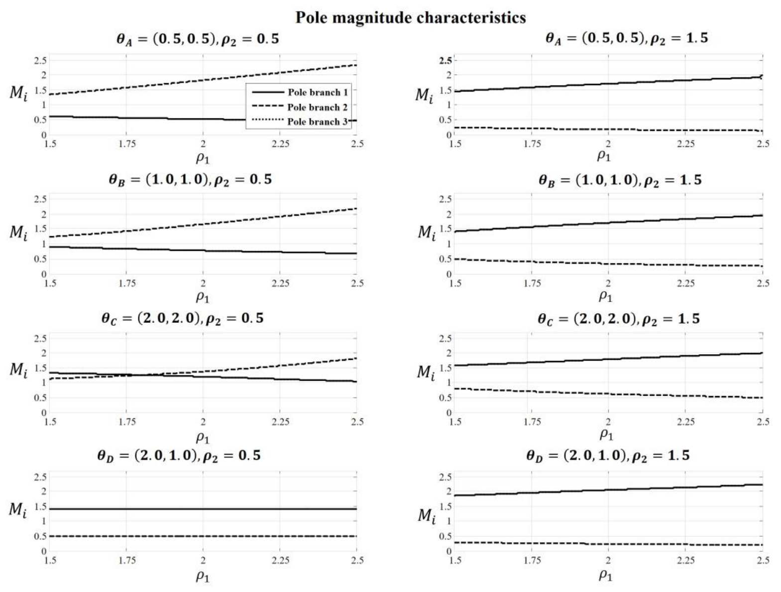
Figure 2.
Modulus characteristics of the tracked pole branches for the tunings θA, θB, θC, and θD as ρ2 varies along the boundary trajectories ρ1 = 1.5 and ρ1 = 2.5.
Figure 2.
Modulus characteristics of the tracked pole branches for the tunings θA, θB, θC, and θD as ρ2 varies along the boundary trajectories ρ1 = 1.5 and ρ1 = 2.5.
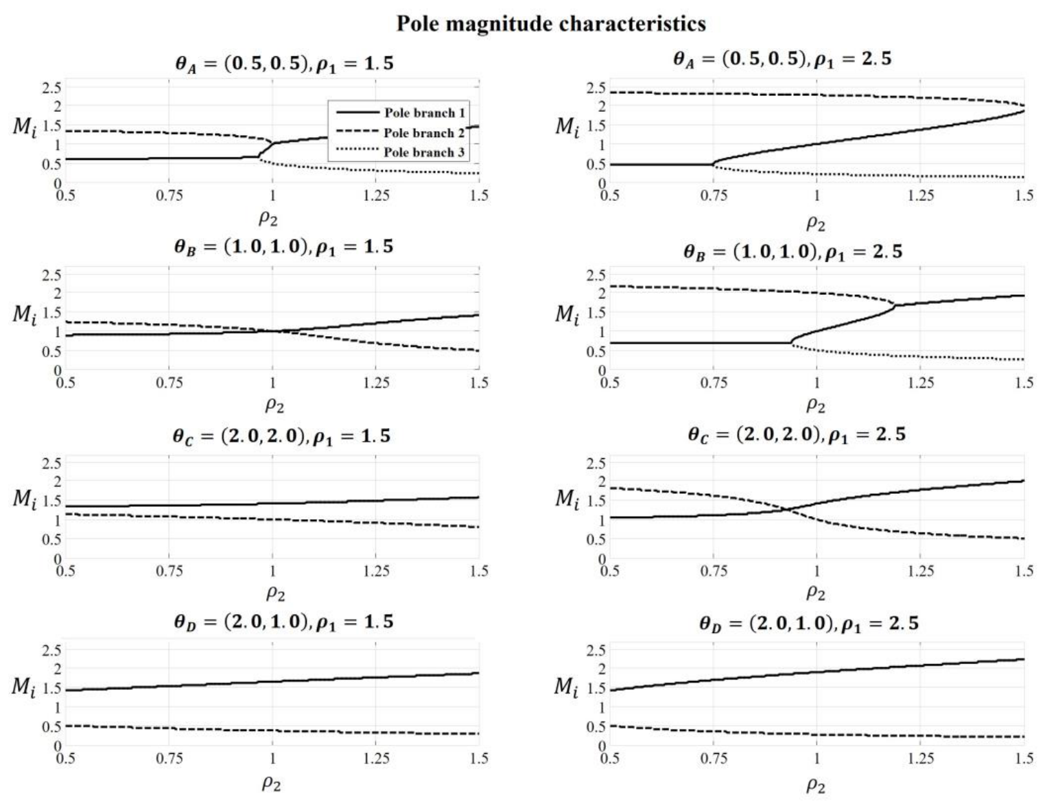
Figure 3.
Phase characteristics of the pole branch with a positive imaginary part for the tunings θA, θB, θC, and θD as ρ1 varies along the boundary trajectories ρ2 = 0.5 and ρ2 = 1.5.
Figure 3.
Phase characteristics of the pole branch with a positive imaginary part for the tunings θA, θB, θC, and θD as ρ1 varies along the boundary trajectories ρ2 = 0.5 and ρ2 = 1.5.
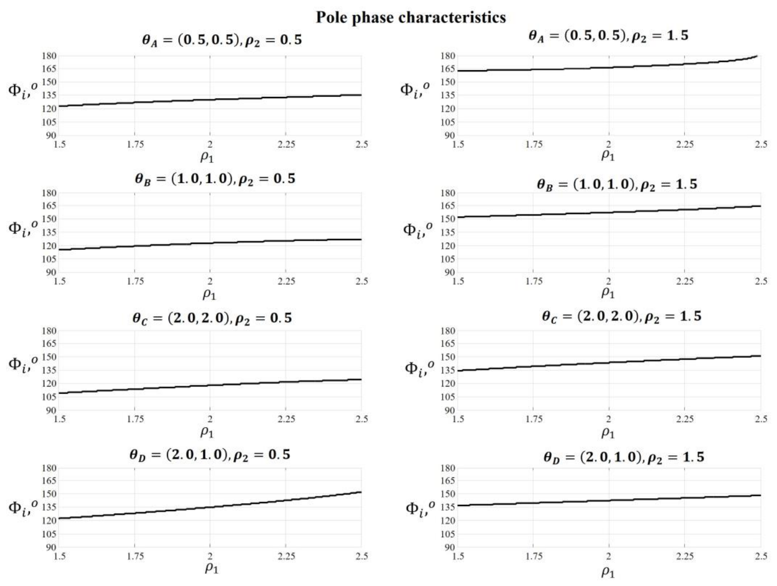
Figure 4.
Phase characteristics of the pole branch with a positive imaginary part for the tunings θA, θB, θC, and θD as ρ2 varies along the boundary trajectories ρ1 = 1.5 and ρ1 = 2.5.
Figure 4.
Phase characteristics of the pole branch with a positive imaginary part for the tunings θA, θB, θC, and θD as ρ2 varies along the boundary trajectories ρ1 = 1.5 and ρ1 = 2.5.
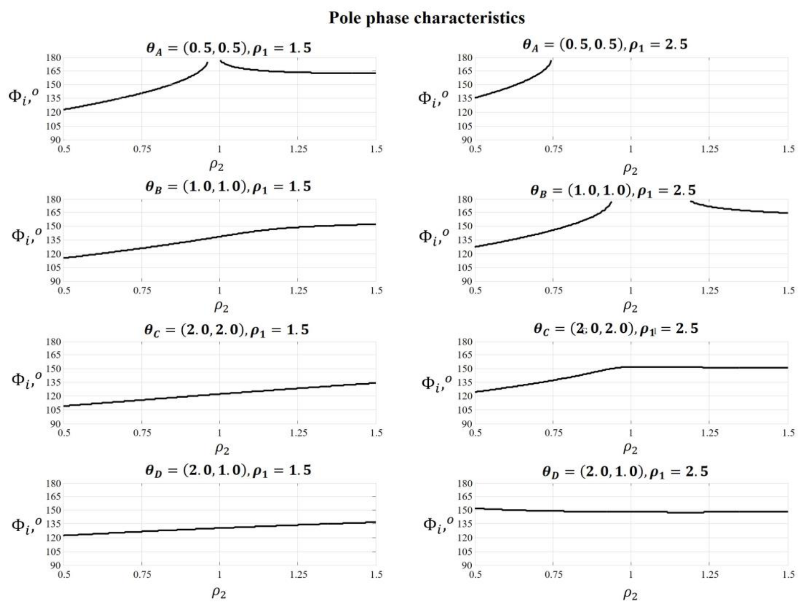
Figure 5.
Modulus, phase, and total sensitivities of the tracked complex pole branch with a positive imaginary part with respect to ρ1 for the tunings θA, θB, θC, and θD at ρ2 = 0.5 and ρ2 = 1.5.
Figure 5.
Modulus, phase, and total sensitivities of the tracked complex pole branch with a positive imaginary part with respect to ρ1 for the tunings θA, θB, θC, and θD at ρ2 = 0.5 and ρ2 = 1.5.
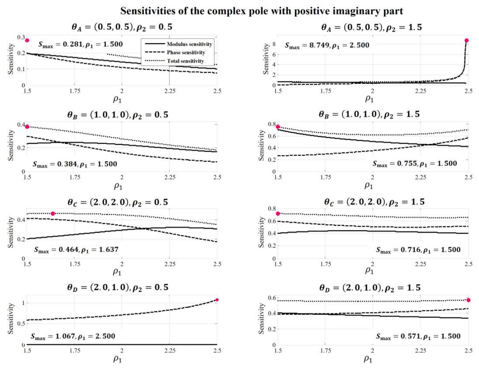
Figure 6.
Modulus, phase, and total sensitivities of the tracked complex pole branch with a positive imaginary part with respect to ρ2 for the tunings θA, θB, θC, and θD at ρ1 = 1.5 and ρ1 = 2.5.
Figure 6.
Modulus, phase, and total sensitivities of the tracked complex pole branch with a positive imaginary part with respect to ρ2 for the tunings θA, θB, θC, and θD at ρ1 = 1.5 and ρ1 = 2.5.
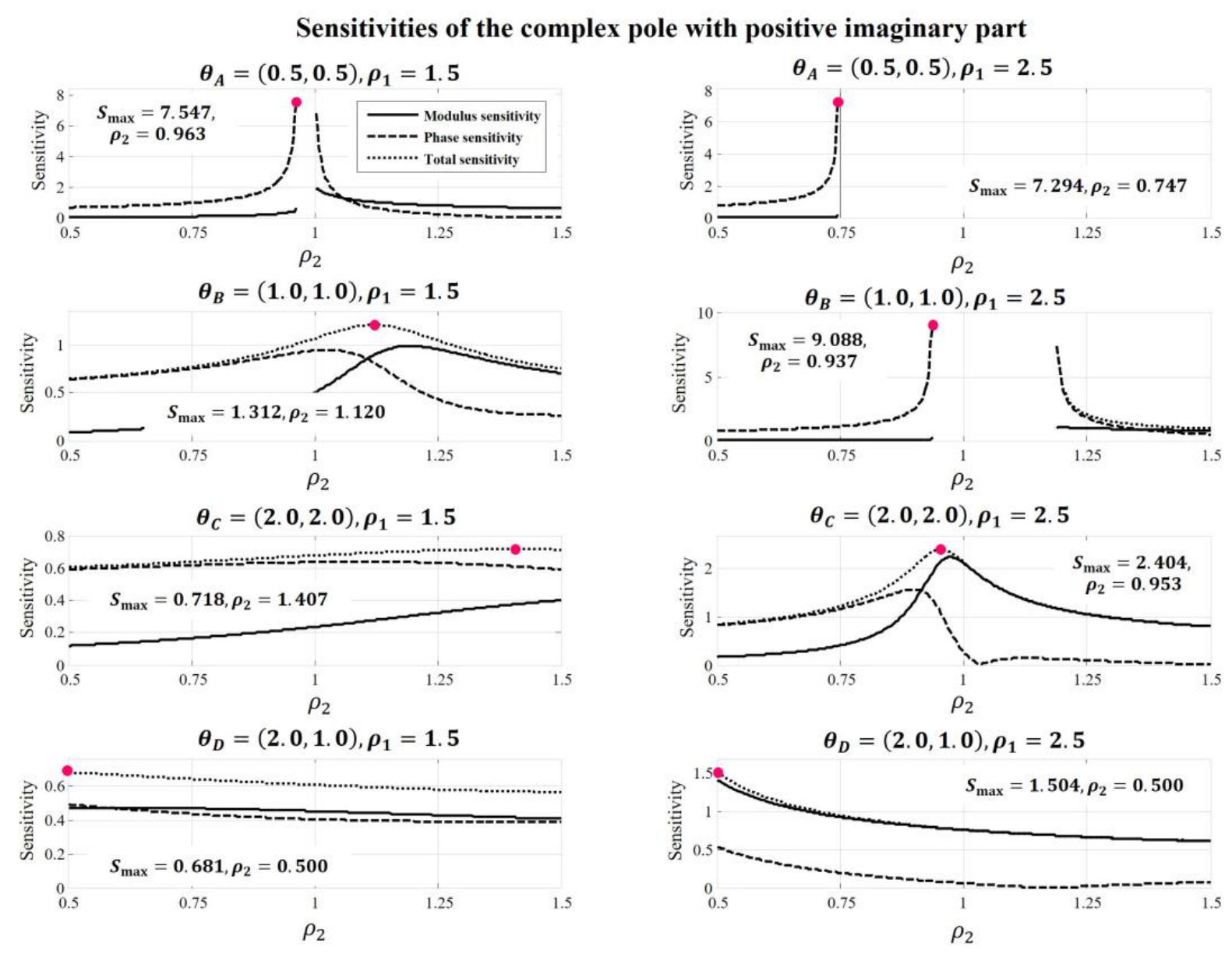
Figure 7.
Sensitivity of the tracked real pole branch with respect to ρ1 and ρ2 for the tunings θA, θB, θC, and θD.
Figure 7.
Sensitivity of the tracked real pole branch with respect to ρ1 and ρ2 for the tunings θA, θB, θC, and θD.
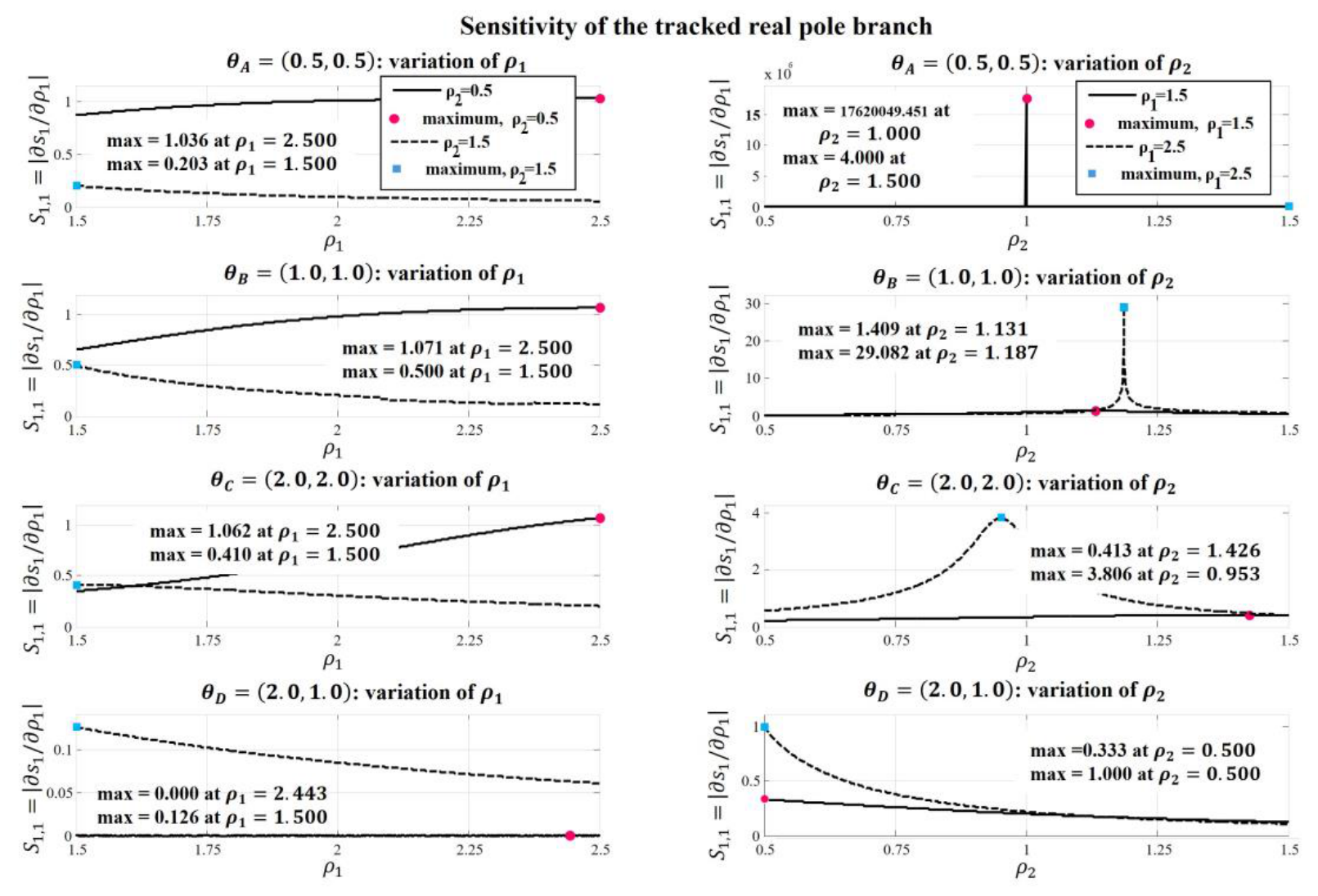
Figure 8.
Root contours of all pole branches for the tunings θA, θB, θC, and θD, mapped according to the numerically determined total pole sensitivity Si,1 with respect to ρ1 θA = (0.5, 0.5). ρ2 = 0.5 and ρ2 = 1.5.
Figure 8.
Root contours of all pole branches for the tunings θA, θB, θC, and θD, mapped according to the numerically determined total pole sensitivity Si,1 with respect to ρ1 θA = (0.5, 0.5). ρ2 = 0.5 and ρ2 = 1.5.
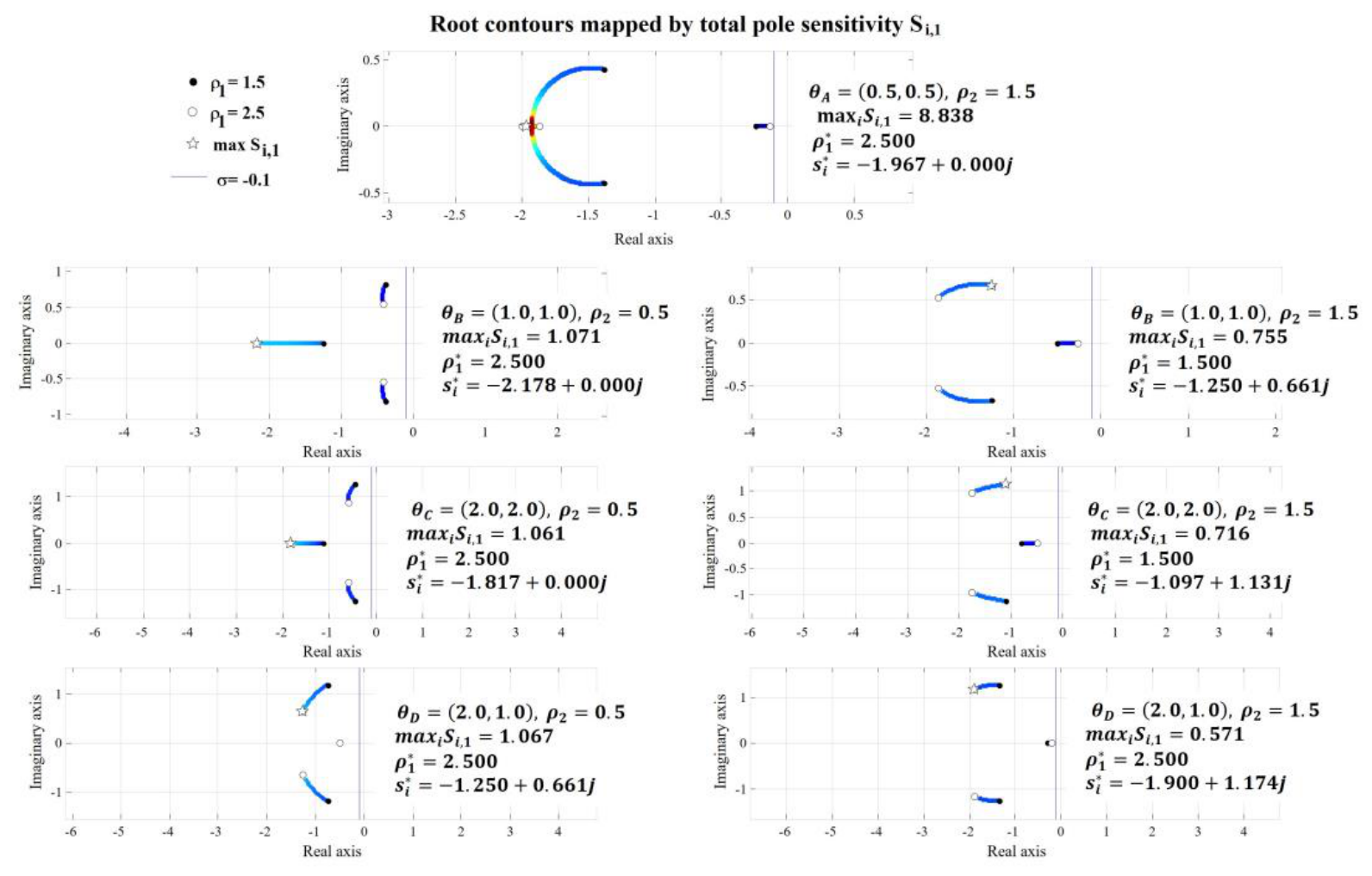
Figure 9.
Root contours of all pole branches for the tunings θA, θB, θC, and θD, mapped according to the numerically determined total pole sensitivity Si,2 with respect to ρ2 at ρ1 = 1.5 and ρ1 = 2.5.
Figure 9.
Root contours of all pole branches for the tunings θA, θB, θC, and θD, mapped according to the numerically determined total pole sensitivity Si,2 with respect to ρ2 at ρ1 = 1.5 and ρ1 = 2.5.
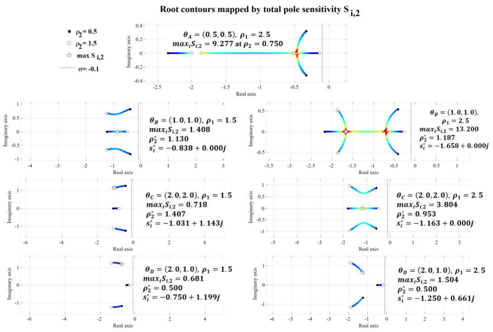
Figure 10.
Positions of all poles for the tunings θA, θB, θC, and θD, mapped according to the overall local indicator Si,max = σmax(Ji) over the parametric region Ωρ.
Figure 10.
Positions of all poles for the tunings θA, θB, θC, and θD, mapped according to the overall local indicator Si,max = σmax(Ji) over the parametric region Ωρ.
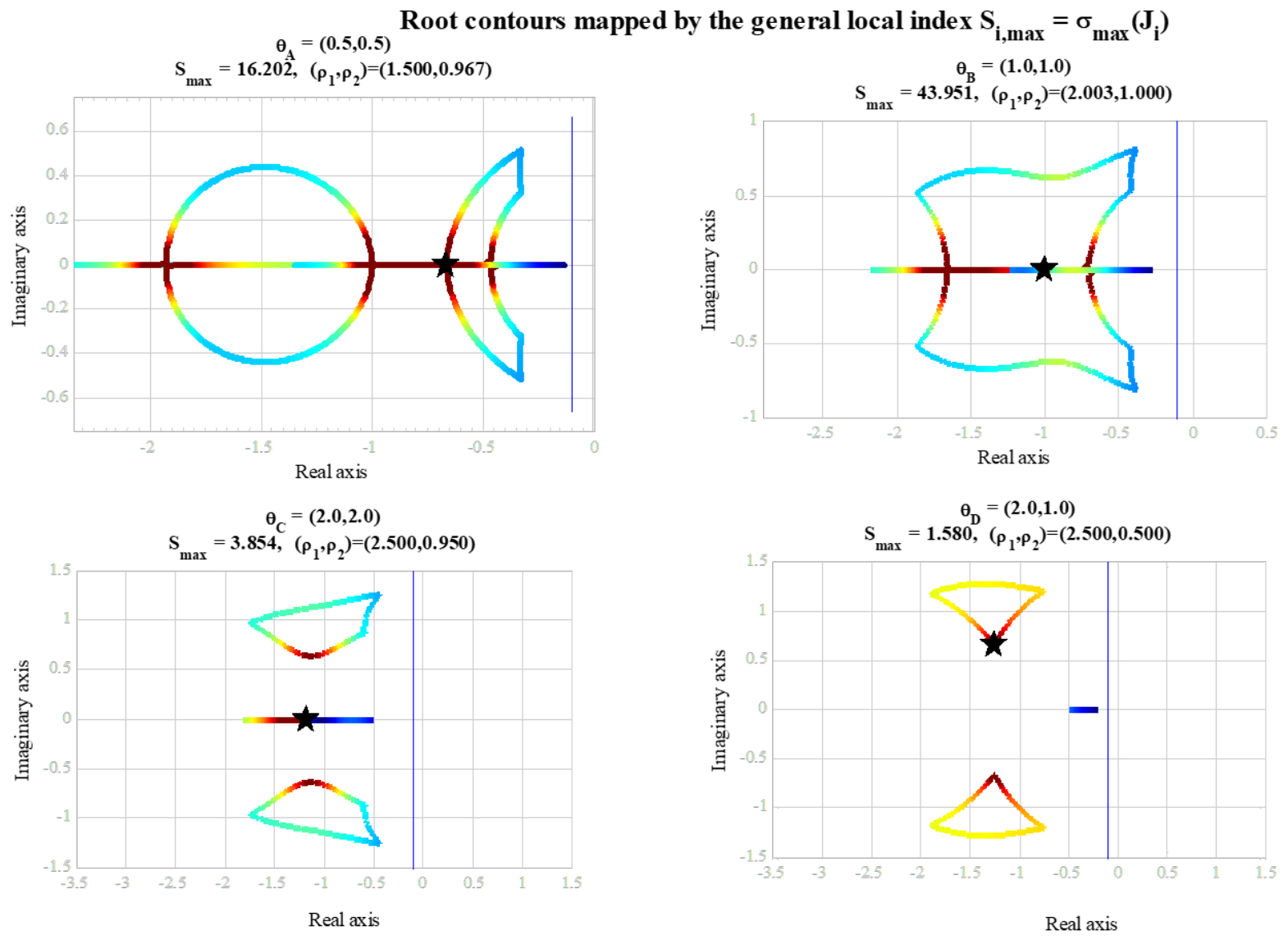
Figure 11.
Separate mapping of the modulus sensitivity SM,1,2 and phase sensitivity SΦ,1,2 onto the same tracked complex pole branch with a positive imaginary part.
Figure 11.
Separate mapping of the modulus sensitivity SM,1,2 and phase sensitivity SΦ,1,2 onto the same tracked complex pole branch with a positive imaginary part.
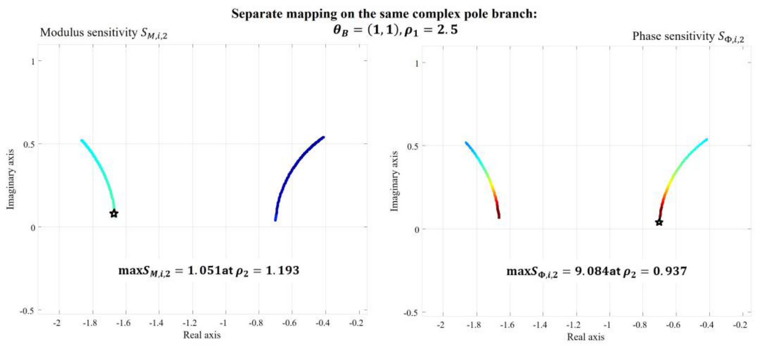
Figure 12.
Normalized comparison of the global indicators, local pole sensitivity, and transient-response sensitivity for the seven robustly admissible PI tunings.
Figure 12.
Normalized comparison of the global indicators, local pole sensitivity, and transient-response sensitivity for the seven robustly admissible PI tunings.
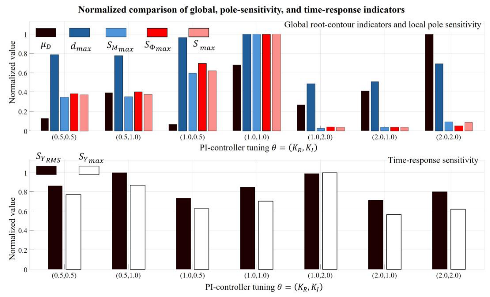
Figure 13.
Family and envelope of the transient responses for the robustly admissible PI tuning (KR, KI) = (2, 1).
Figure 13.
Family and envelope of the transient responses for the robustly admissible PI tuning (KR, KI) = (2, 1).
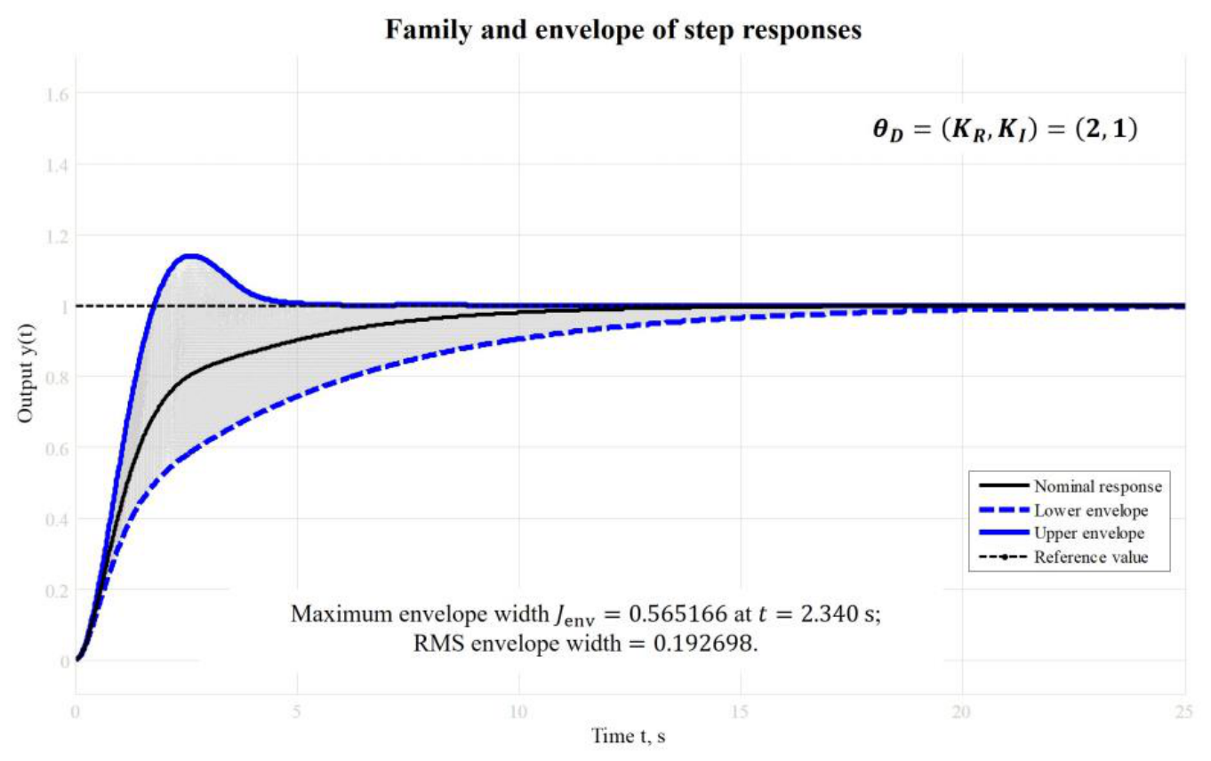
Figure 14.
Family and envelope of the transient responses for the robustly admissible PI tuning (KR, KI) = (1, 2).
Figure 14.
Family and envelope of the transient responses for the robustly admissible PI tuning (KR, KI) = (1, 2).
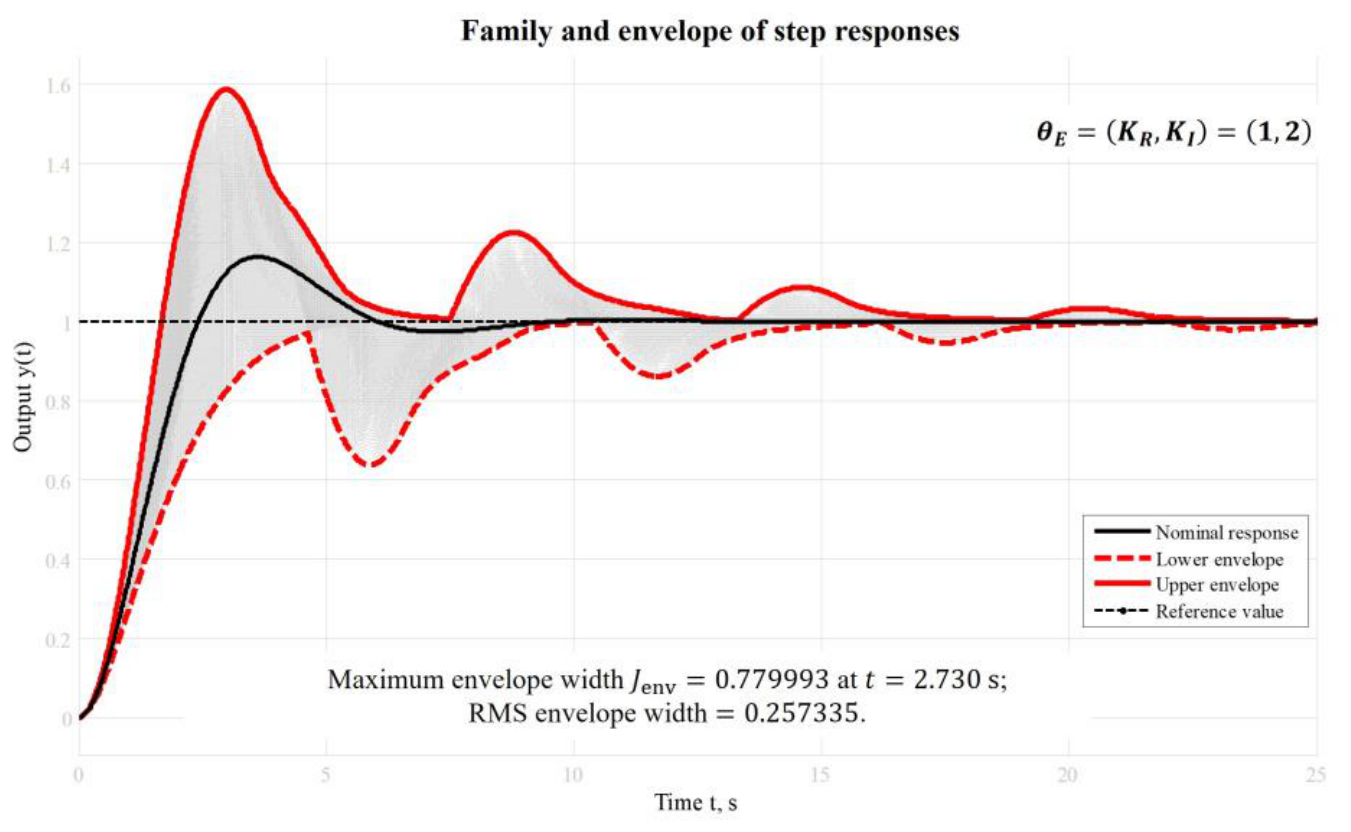
Figure 15.
Direct comparison of the transient-response envelopes for the tunings (KR, KI) = (2, 1) and (KR, KI) = (1, 2).
Figure 15.
Direct comparison of the transient-response envelopes for the tunings (KR, KI) = (2, 1) and (KR, KI) = (1, 2).
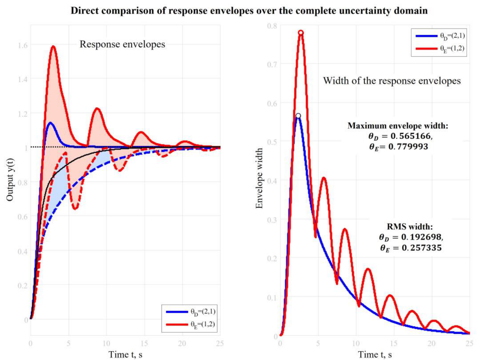

Table 1.
Summary of the maximum modulus, phase, and total pole sensitivity values of the complex pole branch along the considered boundary trajectories.
Table 1.
Summary of the maximum modulus, phase, and total pole sensitivity values of the complex pole branch along the considered boundary trajectories.
| Tuning | Varied Parameter | Fixed Parameter | Critical Value | Critical Value | Critical Value | |||
|---|---|---|---|---|---|---|---|---|
| θA | ρ1 | ρ2 = 0.5 | 0.1973 | ρ1 = 1.500 | 0.1996 | ρ1 = 1.500 | 0.2806 | ρ1 = 1.500 |
| ρ1 | ρ2 = 1.5 | 0.6124 | ρ1 = 1.500 | 8.7358 | ρ1 = 2.490 | 8.7487 | ρ1 = 2.490 | |
| ρ2 | ρ1 = 1.5 | 1.8561 | ρ2 = 1.007 | 7.5233 | ρ2 = 0.963 | 7.5466 | ρ2 = 0.963 | |
| ρ2 | ρ1 = 2.5 | 0.2031 | ρ2 = 0.747 | 7.2912 | ρ2 = 0.747 | 7.2940 | ρ2 = 0.747 | |
| θB | ρ1 | ρ2 = 0.5 | 0.2486 | ρ1 = 1.713 | 0.3011 | ρ1 = 1.500 | 0.3836 | ρ1 = 1.500 |
| ρ1 | ρ2 = 1.5 | 0.7058 | ρ1 = 1.500 | 0.5627 | ρ1 = 2.500 | 0.7548 | ρ1 = 1.500 | |
| ρ2 | ρ1 = 1.5 | 0.9897 | ρ2 = 1.193 | 0.9512 | ρ2 = 1.027 | 1.2116 | ρ2 = 1.120 | |
| ρ2 | ρ1 = 2.5 | 1.0510 | ρ2 = 1.193 | 9.0838 | ρ2 = 0.937 | 9.0884 | ρ2 = 0.937 | |
| θC | ρ1 | ρ2 = 0.5 | 0.3205 | ρ1 = 2.293 | 0.4160 | ρ1 = 1.500 | 0.4641 | ρ1 = 1.637 |
| ρ1 | ρ2 = 1.5 | 0.4389 | ρ1 = 1.863 | 0.5933 | ρ1 = 1.500 | 0.7162 | ρ1 = 1.500 | |
| ρ2 | ρ1 = 1.5 | 0.4011 | ρ2 = 1.500 | 0.6411 | ρ2 = 1.097 | 0.7185 | ρ2 = 1.407 | |
| ρ2 | ρ1 = 2.5 | 2.2429 | ρ2 = 0.973 | 1.5704 | ρ2 = 0.900 | 2.4038 | ρ2 = 0.953 | |
| θD | ρ1 | ρ2 = 0.5 | 0.0013 | ρ1 = 2.500 | 1.0665 | ρ1 = 2.500 | 1.0665 | ρ1 = 2.500 |
| ρ1 | ρ2 = 1.5 | 0.4071 | ρ1 = 1.500 | 0.4584 | ρ1 = 2.500 | 0.5710 | ρ1 = 2.500 | |
| ρ2 | ρ1 = 1.5 | 0.4739 | ρ2 = 0.600 | 0.4913 | ρ2 = 0.500 | 0.6807 | ρ2 = 0.500 | |
| ρ2 | ρ1 = 2.5 | 1.4069 | ρ2 = 0.500 | 0.5312 | ρ2 = 0.500 | 1.5038 | ρ2 = 0.500 |
Table 2.
Comparison of local pole sensitivity and transient-response sensitivity for the seven robustly admissible PI tunings.
Table 2.
Comparison of local pole sensitivity and transient-response sensitivity for the seven robustly admissible PI tunings.
| KR | KI | SM,max | SΦ,max | Smax | Sy,RMS | Sy,max | Relative Assessment |
|---|---|---|---|---|---|---|---|
| 0.5 | 0.5 | 14.514 | 14.065 | 16.202 | 0.519193 | 0.893356 | Robustly admissible, with an exact multiple root and moderate time-domain sensitivity |
| 0.5 | 1.0 | 14.724 | 14.839 | 16.414 | 0.602920 | 1.012428 | Robustly admissible, with an exact multiple root within the uncertainty region and high time-domain sensitivity |
| 1.0 | 0.5 | 24.976 | 25.691 | 27.312 | 0.441414 | 0.727801 | Robustly admissible, with an exact multiple root within the uncertainty region but low time-domain sensitivity |
| 1.0 | 1.0 | 42.221 | 36.902 | 43.951 | 0.509881 | 0.819799 | Robustly admissible, with an exact multiple root within the uncertainty region and moderate time-domain sensitivity |
| 1.0 | 2.0 | 0.883 | 1.388 | 1.388 | 0.594724 | 1.163005 | Robustly admissible, with low pole sensitivity but high time-domain sensitivity |
| 2.0 | 1.0 | 1.407 | 1.191 | 1.580 | 0.428249 | 0.654165 | Robustly admissible, with low pole sensitivity and the lowest time-domain sensitivity |
Disclaimer/Publisher’s Note: The statements, opinions and data contained in all publications are solely those of the individual author(s) and contributor(s) and not of MDPI and/or the editor(s). MDPI and/or the editor(s) disclaim responsibility for any injury to people or property resulting from any ideas, methods, instructions or products referred to in the content. |
© 2026 by the authors. Licensee MDPI, Basel, Switzerland. This article is an open access article distributed under the terms and conditions of the Creative Commons Attribution (CC BY) license (http://creativecommons.org/licenses/by/4.0/).
Copyright: This open access article is published under a Creative Commons CC BY 4.0 license, which permit the free download, distribution, and reuse, provided that the author and preprint are cited in any reuse.