
Submitted:
02 September 2026
Posted:
03 September 2026
You are already at the latest version
Abstract
Existing methods for human action recognition from dynamic point clouds commonly rely on farthest point sampling and dense spatiotemporal neighborhood queries. The resulting local geometric computations are expensive, which complicates deployment in resource-constrained settings. This paper presents the Global–Local Differencing Network (GLD-Net), a lightweight framework for point-cloud sequence learning designed around feature extraction, motion representation, and temporal modeling. Feature extraction uses a two-branch architecture: the global branch encodes the complete point cloud in each frame to learn a holistic spatial representation, whereas the local branch uniformly divides the body along the vertical direction into several semantic regions, each processed by an independent network. Motion is represented directly by the distances from each point to its nearest neighbors in the preceding and subsequent frames, without requiring point correspondences. For temporal modeling, bidirectional differencing is applied to frame-level features to represent action changes explicitly. The method requires neither farthest point sampling nor complex spatiotemporal neighborhood searches. On MSR-Action3D, GLD-Net achieves 95.82% accuracy with 0.579 M parameters and 1.42 G operations. Compared with PvNeXt, a model of similar scale, GLD-Net improves accuracy by 1.05 percentage points while reducing the parameter count by 19.6%.The implementation code is publicly available at https://github.com/daidai321/GLD-Net.
Keywords:
human action recognition
; dynamic point clouds
; global and local feature fusion
; nearestneighbor motion representation
1. Introduction
Human action recognition supports applications such as human–computer interaction, rehabilitation assessment, ambient intelligence, and security surveillance. Depth sensors provide a practical compromise between RGB appearance and skeletal abstraction. They are insensitive to illumination changes and capture metric scene geometry, without requiring texture-rich images to be stored or relying on a pose estimator. Converting a depth sequence produces a dynamic point cloud, in which each frame is an unordered set of three-dimensional points. Early depth-based action-recognition methods mostly operated on depth images and represented temporal changes using two-dimensional representations, including histograms of oriented normals, dynamic images, and structured depth images [1–3]. With advances in deep learning for point clouds [4,5], recent research has shifted markedly toward action-recognition methods that model three-dimensional point clouds directly [6–13], thereby recasting action recognition as a point-cloud sequence modeling problem.
The lack of stable point correspondences is a central obstacle in dynamic point-cloud modeling. Most current methods address this issue by constructing local spatiotemporal neighborhoods. MeteorNet performs feature aggregation directly on dynamic point sets [6]; P4Transformer and PSTNet combine spatial grouping with temporal aggregation [7,8]; and PST-Transformer enhances the representation using displacement-aware attention [9]. More recent studies have explored feature-level surfaces [10], minimalist pointwise architectures [11], state-space models [12], spectral-domain mixing [13], point-relationship guidance [33], and hierarchical collaboration [34]. Despite following different technical routes, most of these methods retain the same underlying paradigm of local geometric construction. They rely on intensive farthest point sampling, anchor grouping, and overlapping neighborhood queries, resulting in high overall computational cost. A single descriptor obtained by global pooling can substantially reduce computation, but discriminative information from subtle movements of body parts such as the arms and legs can be obscured. Existing methods essentially couple spatial locality with motion modeling by relying on detailed local-neighborhood searches to capture motion implicitly. This raises two questions: if motion cues can be obtained explicitly and more directly, can the requirement for spatial locality be substantially relaxed, and how far can the model be simplified?
To address these questions, this paper proposes the Global–Local Differencing Network (GLD-Net). Its central idea is to decouple motion extraction from spatial locality by replacing implicit local-geometric learning with explicit motion measures and fine-grained neighborhood searches with coarse body partitions. The model has three main components. For feature extraction, it uses global and local branches. The global branch represents the complete point cloud in each frame, whereas the local branch uniformly divides the body along the vertical direction into several semantic regions and encodes each region with an independent pointwise network. This coarse decomposition along the body axis retains discriminative cues from important regions such as the arms and legs while avoiding the cost of farthest point sampling and ball queries. The local features are aggregated by attention and paired frame by frame with the global features, after which a temporal Transformer models them jointly. For motion representation, the distances from each point to its nearest neighbors in the preceding and subsequent frames directly describe its motion state: stationary regions produce small matching distances, whereas moving limbs produce large residuals. This representation requires neither point correspondences nor learnable parameters. For temporal modeling, bidirectional differencing is applied to frame-level features to incorporate action changes explicitly. The temporal Transformer can therefore focus on recognizing action patterns rather than deriving motion from static frames. The complete framework requires no farthest point sampling, ball queries, or learnable four-dimensional neighborhood construction.
The main experiments are conducted on MSR-Action3D [55]. GLD-Net achieves 95.82% recognition accuracy with 0.579 M parameters and 1.42 G operations. Compared with PvNeXt [11], a recent model of similar scale, GLD-Net achieves 1.05 percentage points higher accuracy with 19.6% fewer parameters. Figure 1 shows the positions of the selected models and representative methods in the accuracy–parameter plane. To facilitate reproducibility, the implementation code is publicly available at https://github.com/daidai321/GLD-Net.
The main contributions of this paper are as follows:
- 1.
- A two-branch global and local feature extraction scheme is proposed. The global branch represents the complete point cloud in each frame, whereas the local branch uniformly divides the body along the Y-axis and extracts features from each segment independently. Attention-based fusion combines holistic context with local body evidence without requiring any neighborhood-construction operation.
- 2.
- A fast nearest-neighbor motion representation is proposed. It represents motion using the distances from each point to its nearest neighbors in the preceding and subsequent frames. The representation is parameter-free, requires no point correspondences, and can be attached directly to any point-cloud sequence model.
- 3.
- Bidirectional differencing is applied to frame-level features to separate action changes explicitly from static frame features, allowing the temporal Transformer to focus on action-pattern recognition. A constant-parameter ablation protocol is used to verify the independent contribution of each design.
2. Related Work
2.1. Point-Cloud Feature Extraction
PointNet pioneered static point-cloud feature learning by combining a shared pointwise network with symmetric pooling to learn permutation-invariant set representations [4]. Deep Sets and Set Transformer subsequently provided a theoretical formalization of invariance and attention-based set aggregation, respectively [14,15]. PointNet++ introduced local geometry into point-cloud learning through hierarchical sampling and grouping [5]. In parallel with pointwise methods, voxel-based approaches first quantize point clouds into regular grids and then extract features using three-dimensional convolutions [16], at the cost of quantization errors and memory consumption that increases with resolution. Subsequent studies have focused on how to model neighborhoods, including learnable permutations [17], dynamic graphs [18], continuous convolutions [19], deformable kernels [20], and vector attention [21]. Another line of research has shown that residual architectures and carefully designed training strategies can also be effective without introducing complex neighborhood operators [22–24]. Masked point modeling has further extended point-cloud representation learning to the pretraining paradigm [25,26].
Dynamic point-cloud models add temporal associations to these spatial representations. Sparse four-dimensional convolutions process spatiotemporal coordinates on voxel grids [27]. MeteorNet, P4Transformer, PSTNet, and PST-Transformer established the prevalent paradigm of combining spatial grouping with temporal aggregation [6–9], while Kinet and PSTNet++ further improved feature-level surfaces and operator decomposition [10,28]. Recent action-recognition models have evolved along several directions, including explicit action structures [29], minimal pointwise designs [11], state-space models [12], spectral-domain modeling [13,30], adaptive decoupling [31], KAN enhancement [32], point-relationship guidance [33], and hierarchical collaboration [34]. Unlike these methods, GLD-Net performs neither iterative nor learnable point-neighborhood construction and organizes spatial information using only one complete point set and three fixed-height segments.
2.2. Motion Representation in Action Recognition
The central issue in action recognition is how to represent motion information. Early depth-based methods mainly made motion explicit in two-dimensional representations, including histograms of normals [1], dynamic images [2], structured depth images [3], HHA encoding [35], and depth-skeleton sequences [36]. Spatial encodings based on orthographic projection have also provided an efficient approach to depth-based human analysis [37–38]. Although these representations are intuitive and effective, they regularize or project the original three-dimensional samples. After the transition to point clouds, one line of research directly estimated dense scene flow between adjacent point sets [39]. For action recognition, however, dense flow constitutes an additional prediction problem and incurs considerable computational and supervision costs. Another line of research characterizes changes at the feature level: rather than requiring a network to infer motion implicitly from static frame features, inter-frame differences can be provided explicitly to the model. The two designs in this paper provide lightweight implementations of these two directions. Nearest-neighbor distances provide only a scalar motion cue without requiring pointwise correspondences; they neither move points, alter labels, nor introduce parameters. Bidirectional feature differencing makes ’action changes’ explicit at the feature level, so that the temporal model does not need to infer the motion process by itself from static frame features.
2.3. Temporal Modeling in Action Recognition
One class of methods that directly models temporal information in raw point-cloud sequences uses pointwise spatiotemporal operators [6–9,27]. These methods maintain high-resolution spatiotemporal feature maps at both point and frame granularities, and pointwise neighborhood searches result in persistently high computational and memory costs. Transformers provide a global receptive field for sequence modeling [40], but their attention cost grows quadratically with the number of tokens. Video Transformers generally control this cost by factorizing spatial and temporal attention or reducing token redundancy [41,42]. For point-cloud sequences, treating every point as a token would make this cost prohibitive. Representing each complete frame as a token instead makes the scale of temporal modeling independent of the number of points per frame, providing a natural choice that balances efficiency and global dependencies. Following this idea, GLD-Net compresses each frame into one global token and one local token. The attention-weighted aggregation of local features is related to attention-based multiple-instance learning [43], except that the ’instances’ here are differenced segment-level frame features rather than image patches.
3. Methods
The complete pipeline of GLD-Net is shown in Figure 2. For every point in each frame point cloud (), the network first computes its nearest-neighbor (NN) distances and to the preceding and succeeding frame point clouds. After frame-wise normalization, these distances are concatenated with the three-dimensional coordinates of the point itself and a normalized temporal feature to form a six-dimensional input (). Global and local networks then extract features separately. The global network directly encodes the complete input using PointNet, whereas the local network partitions the human point cloud into K segments along the Y-axis ( on MSR-Action3D in this paper) and extracts features from them using mutually independent PointNets. The features in each stream are bidirectionally differenced from the corresponding-stream features of the preceding and succeeding frames, making ’action changes’ explicit at the feature level. The K differenced local features are then aggregated into one local token through attention weighting. Finally, each frame retains two independent tokens, one global and one local. A temporal Transformer captures temporal associations throughout the complete sequence through self-attention and maps them to an action prediction. The complete network constructs no point-level neighborhoods, while integrating three complementary cues: global structure, local structure, and motion changes.
3.1. Input Representation and Preprocessing
Action recognition on point-cloud sequences can be formulated as follows: given a point-cloud sequence back-projected from consecutive depth frames, predict the action category to which the sequence belongs. For a clip containing T frames, the tth frame contains N three-dimensional points, denoted by , where . All coordinates are uniformly divided by 300 for scale normalization. This normalization does not involve centroid alignment, and the relative displacement between frames is therefore fully preserved. Each frame is resampled to 2048 points. When more than 2048 points are available, points are randomly sampled without replacement; when fewer points are available, the points are cyclically repeated and the remainder is filled by random sampling.
3.2. Point-Level Bidirectional Nearest-Neighbor Motion Representation
Points are unordered, so inter-frame motion cannot be computed by direct index-wise subtraction as in grid-based videos. For each point , its minimum distances to the preceding and succeeding point sets are therefore defined as the backward and forward residuals, respectively, as shown in Equation (1):
Here, is the ith point in the tth frame, the index j traverses all points in the adjacent-frame point set, denotes the Euclidean distance, and and are the minimum distances from this point to the preceding and succeeding point sets, respectively. At temporal boundaries, only the available one-sided adjacent frame is used. The two distance fields are separately normalized within each frame, as shown in Equation (2):
Here, the index l traverses all points in the tth frame, is a very small constant that prevents division by zero, and the normalized value is the nearest-neighbor motion representation of the point. This operation contains no parameters and requires neither optical-flow ground truth nor point correspondences. A larger distance indicates that the point is more difficult to explain using the adjacent point set and is therefore more likely to lie on a moving surface, a newly visible region, or a boundary affected by motion.
The nearest-neighbor search in Equation (1) is implemented by brute force. For each frame, the distance matrix between it and an adjacent frame is directly computed, and the minimum is then taken along the adjacent-frame point dimension. Its computational complexity is , making it the only quadratic term in the complete model. This step contains no parameters, requires no backpropagation, and is implemented as a single batched matrix operation on a GPU. The measured per-clip inference latency reported in Section 4.2 fully includes this computation. Compared with iterative neighborhood-construction operations such as farthest point sampling and ball query, it has a higher asymptotic complexity but requires only a single execution and can be fully parallelized.
The final six-dimensional point descriptor is given by Equation (3):
where is the six-dimensional descriptor of point ; , , and are its three-dimensional coordinates; and is the normalized temporal feature, namely, the relative position of the frame index within the clip. The nearest-neighbor search and construction of the six-dimensional descriptor are illustrated in Figure 3.
3.3. Global and Local Feature Extraction
The complete frame is encoded by a global pointwise network . Because actions occur primarily in body parts such as the arms and legs, body-part-level local information is introduced by uniformly dividing the interval along the Y-axis, corresponding to the human height direction, into non-overlapping segments. In ascending order of the Y-coordinate, these segments are denoted by , , and , and points outside the interval are assigned to the nearest boundary segment. Here, and H are constants defined in the normalized coordinates described in Section 3.1. On MSR-Action3D, and , covering the height range of the human bodies in this dataset. The segment boundaries are therefore fixed throughout the complete dataset and do not adapt to individual frames or samples, thereby avoiding segment jitter introduced by frame-wise statistics. The specific values of K, D, and other parameters presented in this section correspond to the MSR-Action3D configuration; the corresponding values for NTU RGB+D 60 are given in Section 4.5. Each segment uses an independent encoder without parameter sharing because the upper, middle, and lower segments differ markedly in body structure and motion patterns. All encoders operate directly on the six-dimensional point attributes, as shown in Equation (4):
Here, max denotes channel-wise max pooling, is the set of points in the kth segment, and and are the global feature and the local feature of the kth segment in the tth frame, respectively. The layer widths of the global encoder are 6–64–128–128. The layer widths of each local encoder are only 6–32–32–128, directly producing a 128-dimensional feature vector rather than first concatenating several narrow vectors and then expanding their dimensionality. Both types of encoder consist of three linear layers. The first two layers are followed by GELU activations, the final layer has no activation, and batch normalization is not used at any stage. If a segment contains no points in a frame, its feature vector is set to zero. Unlike PointNet++-style grouping, the three segments are fixed and non-overlapping, requiring neither anchor-point sampling nor radius-based search. Local structure is therefore introduced with almost no additional cost.
3.4. Feature-Level Bidirectional Differencing
After the encoding described in Section 3.3, each frame yields streams of 128-dimensional features: one global feature and K local features . These features describe only the static form of a single frame, and changes between frames have not yet been represented explicitly. This section applies bidirectional temporal differencing to each feature stream, directly computing ’action changes’ for the subsequent Transformer rather than requiring it to infer motion from static frame features by itself. Specifically, let index the feature streams. Each stream is subtracted from the corresponding-stream features frames earlier and frames later, as shown in Equation (5):
where and are the backward and forward differences of the sth feature stream, respectively, and is the temporal interval. We use throughout the paper, so that differencing is performed over a longer temporal range than adjacent frames while the interval remains much shorter than the 24-frame window. This value is fixed in all experiments and is not tuned separately for individual datasets. Unavailable differences at the boundaries are set to zero. For each stream, the current feature, backward difference, and forward difference are concatenated into a 384-dimensional vector and then mapped back to 128 dimensions as the final frame feature of that stream. The global stream uses a direct linear transformation, as shown in Equation (6):
Here, ∥ denotes channel-wise concatenation, and are learnable weights and biases, and is the final frame feature of the global stream. The three local streams do not directly apply this transformation but instead use two steps, compression followed by restoration. A linear layer first compresses the feature, followed by GELU activation and dropout [56], and a linear layer then restores the feature dimension. This structure is referred to as a low-rank bottleneck, and its output is denoted by (), which serves as the final frame feature of the kth local stream. The local streams do not use the same one-step transformation as the global stream because experiments showed that such a transformation was difficult to optimize on the small dataset, whereas introducing an intermediate 32-dimensional compression substantially improved training stability. At this point, the network contains explicit motion information at two levels. The nearest-neighbor distances in Section 3.2 measure the geometric non-correspondence of individual points at the input level, whereas the differences in this section measure temporal changes in pooled features at the feature level. The two operate at different levels and are not redundant. The structures used for differencing and mapping in the individual streams are shown in Figure 4.
3.5. Temporal Encoding and Classification
The K local feature streams output by Section 3.4 must be merged into one stream. Rather than using simple concatenation or summation, learnable scalar attention is introduced to compute a scalar weight for each local feature. The weights are normalized across the segments using softmax and are then used to form a weighted sum of the features, as shown in Equation (7):
Here, is a learnable scoring vector, denotes normalization along the segment dimension, is the weight of the kth local feature, and is the weighted sum. The weights are learned by the network, allowing different actions to focus on different segments. For a segment that contains no points in a frame in Section 3.3, its feature vector is zero. After the low-rank bottleneck, it still produces a constant output determined by the bias and participates in the normalization in Equation (7). Because the human body is continuously distributed along the Y-axis in both MSR-Action3D and NTU RGB+D 60, empty segments do not occur in the actual data, and no additional mask is applied for this case. The vector is the local feature of the frame. It is paired with the global feature frame by frame, yielding one global token and one local token for each frame and forming the token sequence , which is then passed to the temporal Transformer.
Self-attention itself does not distinguish the order of its inputs, so the model must be explicitly informed of the frame to which each token belongs. A set of learnable temporal embeddings is therefore introduced, and both tokens from the tth frame receive the same vector : , where is the token of type s in the tth frame, , and is the feature dimension. No additional identity embedding is introduced to distinguish the global and local tokens. Temporal information appears in the network at two levels. The scalar in Equation (3) enters the pointwise descriptor, allowing every point to perceive its frame position during encoding, whereas provides frame order to self-attention at the token level. Because the two operate at different granularities, both are retained. Finally, the 24 frames × 2 token types, for a total of 48 tokens, are arranged into a single sequence in temporal order as the encoder input.
The temporal Transformer consists of pre-normalization layers with attention heads and a head dimension of . The layer-wise computations are shown in Equations (8)–():
Here, is the input token sequence of the ℓth layer, LN denotes layer normalization, , , , and are learnable projection matrices, , , and are the query, key, and value of the jth head, respectively, and Concat denotes concatenation of the outputs of the h heads. Equation () includes a GELU activation after the attention output projection . This differs from a standard Transformer encoder, which directly adds the residual after the output projection, and is a design retained in the implementation of this paper. After the tokens are arranged into a single sequence, self-attention computes pairwise associations among all 48 tokens. Each head therefore produces a attention matrix , whose element in row i and column m represents the degree to which the ith token attends to the mth token. Because these 48 tokens span all 24 frames and both global and local token types, this matrix simultaneously covers long-range inter-frame dependencies and interactions between global and local information. After the attention sublayer, each token independently passes through a small multilayer perceptron that first expands the 128-dimensional feature to 256 dimensions, applies a GELU activation, and then compresses it back to 128 dimensions, as shown in Equation (11):
Here, and are the learnable weights of the feed-forward network, and is the output of the attention sublayer. The complete process is shown in Figure 5.
The output of the temporal Transformer remains a set of 48 tokens with 128 dimensions. To obtain a single representation for the complete video clip, the maximum among the 48 tokens is taken for each feature channel and aggregated into a 128-dimensional vector. After layer normalization, dimensionality expansion, and activation, a classification layer maps the vector to scores for the 20 action categories. During evaluation, the softmax probabilities of all windows from the same video are accumulated before the final category is produced. The classification process is given by Equation (12):
Here, z is the pooled clip-level feature, , , and are the learnable weights and bias of the classification head, q is the intermediate hidden vector, and o contains the scores for the 20 action categories.
4. Experiments
4.1. Datasets
Experiments are conducted on the MSR-Action3D dataset [55]. The dataset contains 20 action categories performed by 10 subjects and is recorded as depth-map sequences. We convert the depth maps into point clouds following the procedure described in Section 3.1. Following the common setting used in previous studies [7,8], we adopt a cross-subject split: sequences from subjects 1–5 are used for training, and sequences from subjects 6–10 are used for testing. To ensure comparability, we use the same fixed cross-subject split and benchmark-level model analysis protocol as P4Transformer, PSTNet, PST-Transformer, and PvNeXt [7–9,11]. In addition, Section 4.5 evaluates generalizability on NTU RGB+D 60.
4.2. Implementation Details
Each input clip consists of 24 consecutive frames, with 2048 points sampled from each frame. Following the protocols used in previous studies [7–9], sliding windows are extracted from each sequence during training. During testing, all consecutive 24-frame windows are enumerated, and the softmax probabilities of all windows from the same video are accumulated to obtain the video-level prediction. We report the highest video-level accuracy achieved during each complete 50-epoch training run. Unless otherwise stated, all comparisons, ablations, and parameter sweeps below use the same protocol: the data split, clip length, number of points per frame, window enumeration procedure, and video-level voting remain unchanged, and only the factor under investigation is varied.
Four types of random augmentation are applied to the input clips during training. The first is independent random scaling along each axis, with scaling factors uniformly sampled between 0.9 and 1.1. The second is random rotation around the Y-axis of the human subject, with angles between and . The third is independent random point dropout in each frame. Between one half and all of the points in each frame are randomly retained, with a lower limit of 64 points to prevent individual frames from becoming excessively sparse. The fourth is coordinate jittering, in which zero-mean Gaussian noise with a standard deviation of 0.01 is added to each point. The random scaling and rotation parameters are shared across all frames in a clip, whereas point dropout and coordinate jittering are applied independently to each frame. No augmentation is applied during testing.
The model uses a feature dimension of , three local segments, and a three-layer, eight-head temporal Transformer. The dropout rates at four locations in the network are 0.1 in the low-rank bottleneck of the local stream, 0.2 after local-token attention aggregation, 0.1 within the temporal Transformer, and 0.2 in the classification head. No dropout is used within the pointwise encoders. The model is optimized using SGD with a momentum of 0.9 and a weight decay of . The learning rate is linearly warmed up to 0.01 during the first ten epochs and reduced to one tenth of its previous value at epochs 20 and 30. Training lasts for 50 epochs with a batch size of 24. The complete model contains 578,613 trainable parameters (0.579 M).
On a single NVIDIA RTX 3090, each training epoch takes approximately 45 seconds. Including a complete test-set evaluation at the end of each epoch, each epoch takes approximately 84 seconds, and all 50 epochs require approximately 70 minutes.
Inference efficiency is evaluated using FP32 on a single NVIDIA RTX 3090. With a batch size of 1, the model processes 107 input clips of size per second, with a mean latency of 9.3 ms and peak GPU memory usage of 112 MiB. When the batch size is increased to 24, throughput increases to 145 clips per second. The latency, throughput, and memory measurements above all correspond to the actual 24-frame input. To ensure consistency with the computation values directly reported for previous methods, Table 1 uses the measured result of the same network configuration with a input: the total computation is 1.42 G.
4.3. Comparison on MSR-Action3D
As shown in Table 1, GLD-Net achieves an accuracy of 95.82% with 0.579 M parameters and 1.42 G computation. The recently proposed PRG-Net and EchoNet are included in the table. EchoNet achieves the highest accuracy, but it contains 6.42 M parameters. Among the methods for which parameter counts are reported, PvNeXt is the only other sub-million-parameter model in the table. Compared with PvNeXt, GLD-Net improves accuracy by 1.05 percentage points while reducing the parameter count by 0.141 M, or 19.6%; its computation increases from 0.55 G to 1.42 G. These results show that the advantage of the proposed method lies in achieving higher accuracy with fewer parameters.
Point-level visualizations of four actions over five adjacent frames are shown in Figure 6. In the nearest-neighbor motion representations in the upper row, the large responses for arm waving and hammering are concentrated on the moving arm, whereas those for side kicking are concentrated on the kicking leg after the kick begins. During jogging, the entire body moves, and the responses spread over the whole body. This occurs because the within-frame normalization in Equation (2) removes the absolute motion magnitude. Although this representation indicates where motion occurs, body-part-level localization still requires local segmentation and feature differencing. The lower row marks the input points that attain the maximum value in channel-wise max pooling. These points are sparsely distributed over locations such as the head, hands, and feet and do not completely coincide with the large-distance regions in the upper row. The nearest-neighbor distance is only an input-level motion measurement; the learned features determine which points support the pooled representation.
4.4. Ablation Experiments
This section evaluates each design of GLD-Net through ablation experiments. We examine the contributions of global and local feature extraction, nearest-neighbor motion representation, and feature differencing, as well as the effects of the number of layers and heads in the temporal Transformer. The component ablations in Table 2 use a constant-parameter protocol. When a component is removed, only its corresponding input is set to zero, or its output is set directly equal to its input; no parameters are deleted. All 0.579 M trainable parameters are therefore retained in the model, allowing the reported performance changes to be attributed to the removed information rather than differences in model capacity. The sweeps over the number of local segments and the temporal Transformer architecture in Table 3 and Table 4 necessarily change the parameter count. Their results are used only to discuss trends in the hyperparameter settings and do not constitute capacity-controlled comparisons. All variants use the same optimizer, data split, sampling procedure, and evaluation protocol.
Global and local features. The accuracy is 92.68% when only global features are used. Adding local features increases the accuracy by 3.14 percentage points to 95.82%, indicating that local motion information and global context are complementary. The effect of the number of segments is shown in Table 3. Three segments produce the highest accuracy, followed closely by four segments at 95.47%. Two segments are too coarse to preserve sufficient local evidence. When the number of segments exceeds four, the accuracy does not continue to improve despite the linear increase in the parameter count. The six- and seven-segment settings degrade substantially, whereas the eight-segment setting partially recovers to 93.03%. This non-monotonic variation indicates that the alignment between uniform segments and body parts interacts with the number of points within each segment. The three-segment setting provides the best balance among localization capability, the number of points within each segment, and model complexity. Following the established evaluation practice of previous point-cloud action-recognition studies on MSR-Action3D, all sensitivity analyses and ablation experiments are conducted using the fixed cross-subject benchmark split. Because the dataset does not provide an official validation-set split, these results should be interpreted as benchmark-level sensitivity analyses rather than independent validation-set estimates.
Nearest-neighbor motion representation. Setting both nearest-neighbor distance channels to zero reduces the accuracy from 95.82% to 88.15%. The resulting decrease of 7.67 percentage points is the largest single-component decrease, indicating that the point-level nearest-neighbor motion representation is the primary source of the model’s discriminative ability.
Feature differencing. Setting the bidirectional feature differences to zero reduces the accuracy to 91.99%, a decrease of 3.83 percentage points. This result indicates that explicitly represented action changes provide information beyond the frame-wise features.
Temporal Transformer. Removing the temporal Transformer reduces the accuracy from 95.82% to 92.33%, a decrease of 3.49 percentage points, indicating that self-attention modeling of inter-frame dependencies is an important source of recognition performance. The effects of depth and number of heads are shown in Table 4. With eight heads, the one-layer encoder achieves 95.47%, which is 0.35 percentage points lower than the three-layer encoder, while using 45.7% fewer parameters. The two-layer encoder achieves 94.08%. The four-layer encoder collapses to 11.85% when trained with the learning rate of 0.01 used for the other configurations. When the learning rate is reduced to 0.001 and all other settings remain unchanged, its accuracy reaches 89.55%, but it remains 6.27 percentage points below the three-layer result. With the depth fixed at three layers, the accuracy increases from 91.99% with two heads to 94.77% with four heads and 95.82% with eight heads. Therefore, the final model uses a three-layer, eight-head temporal Transformer.
4.5. Generalization Validation on NTU RGB+D 60
All preceding experiments are conducted on MSR-Action3D. To examine the feasibility of the proposed design on a larger dataset, we conduct a validation experiment on NTU RGB+D 60 [57]. The dataset was recorded by three cameras in 17 acquisition setups and contains 56,880 videos of 60 action categories performed by 40 subjects. Following the official cross-subject protocol, 40,320 videos are used for training and 16,560 videos are used for testing. The point clouds are back-projected from the officially provided masked human depth maps, consistent with previous studies [7,8,11].
The official masked depth maps still contain residual ground points around the feet and body boundaries. Because each combination of acquisition setup and camera corresponds to a fixed camera position, we calibrate one ground plane for each of the 17 setups × 3 cameras, giving 51 viewpoints in total. For each viewpoint, several spatially distributed ground points are manually selected in one depth frame, and a plane is fitted using RANSAC. The fitted plane is then automatically applied to all sequences from that viewpoint. It is used both to remove ground points and to transform the point cloud into a ground-referenced world coordinate system [38], so that the Y-coordinate directly represents height above the ground. Because the comparison methods do not perform this step, we report results under two input conditions: using only the officially provided masked depth maps, which are the inputs used by the comparison methods, and removing the ground points from these inputs.
Implementation setting. Because NTU RGB+D 60 contains substantially more classes and data than MSR-Action3D, the feature dimension is increased to , and the number of local segments is increased to . The remaining architecture is unchanged, with a three-layer, eight-head temporal Transformer and . The complete model contains 2,200,861 trainable parameters (2.20 M). Because the point clouds have been transformed into a ground-referenced coordinate system, the segmentation interval is no longer defined using constants in normalized coordinates. Instead, it is set directly according to height above the ground, with and m. Each of the five segments covers 0.4 m, giving the correspondence with body parts a clear physical meaning. Each clip still contains 24 frames × 2048 points. Unlike the sliding-window protocol in Section 4.2, four randomly segmented samples are drawn from each video during training, giving 161,280 clips in total. During testing, one deterministic segmented sample is drawn from each video, giving 16,560 clips in total. The prediction of this clip is used directly as the video-level result without multi-window voting. Training augmentation includes frame-wise point dropout after sampling, with a minimum retention ratio of 0.5; rotation of around the Y-axis; mirroring with a probability of 0.5; tilting by around the X- and Z-axes; and random scaling. These augmentations are stronger overall than those used on MSR-Action3D. The classification-head dropout is set to 0.25, and no dropout is used in the pointwise encoders. The optimizer and learning-rate schedule are exactly the same as those in Section 4.2: SGD with a momentum of 0.9 and a weight decay of ; the learning rate is linearly warmed up to 0.01 during the first ten epochs and reduced to one tenth of its previous value at epochs 20 and 30. Training lasts for 40 epochs with a batch size of 24.
As shown in Table 5, GLD-Net achieves 83.27% accuracy under exactly the same input conditions as the other methods. Removing only the residual ground points from the input increases the accuracy to 86.63%. This experiment quantifies a structural property of the proposed method. Because GLD-Net does not construct point neighborhoods, its frame-level descriptor depends on whole-frame pointwise max pooling, while the fixed-height segmentation provides only a coarse spatial partition. It therefore cannot effectively separate background points from human-body points, causing background noise to compete directly with evidence of human motion. In contrast, dense-neighborhood methods naturally exclude distant background points from local regions through anchor grouping and radius search. The cost in accuracy comes with lower computation: the per-clip computation of GLD-Net is 2.23 G, the lowest in the table, at approximately of that of PvNeXt, of that of PSTNet, and of that of P4Transformer and PST-Transformer.
4.6. Discussion
The ablation results show that global features alone achieve 92.68% accuracy. Introducing local features increases the accuracy by 3.14 percentage points, demonstrating the importance of local body-part evidence for action discrimination. The nearest-neighbor motion representation and feature differencing explicitly encode motion information in the input and feature spaces, respectively. Removing the nearest-neighbor motion representation alone reduces the accuracy by 7.67 percentage points, whereas removing feature differencing alone reduces it by 3.83 percentage points. Compared with the lightweight model PvNeXt at the same level, GLD-Net reduces the parameter count by 19.6% while improving the accuracy by 1.05 percentage points, thereby reducing model complexity while improving recognition performance. In addition, GLD-Net provides efficient training and inference: complete training takes approximately 70 minutes on a single RTX 3090, and the per-clip inference latency for a 24-frame input is less than 10 ms.
5. Conclusions
This paper proposed GLD-Net, a lightweight model for action recognition from point-cloud sequences. The model uses the distances from each point to its nearest neighbors in the preceding and subsequent frames as a parameter-free motion representation that requires no point correspondences. A global branch and three local branches defined by vertical partitions extract frame-level features. Bidirectional differencing then represents action changes explicitly, and a temporal Transformer performs the final sequence modeling. The complete process requires neither farthest point sampling nor neighborhood queries. On MSR-Action3D, GLD-Net achieves 95.82% accuracy with 0.579 M parameters and 1.42 G operations. Compared with the lightweight PvNeXt, the proposed method achieves 1.05 percentage points higher accuracy with 19.6% fewer parameters. Constant-parameter ablation experiments show that removing the local features, nearest-neighbor motion representation, and feature differencing decreases accuracy by 3.14, 7.67, and 3.83 percentage points, respectively.
These results show that explicit nearest-neighbor motion representation and global–local feature fusion can replace dense spatiotemporal neighborhood computations with little parameter overhead. The experiments on NTU provide preliminary evidence that this computational advantage can be retained on a larger dataset.
Author Contributions
Conceptualization, F.T. and Y.M.; methodology, F.T. and Y.M.; software, F.T.; validation, F.T.; formal analysis, F.T.; investigation, F.T.; data curation, F.T.; writing—original draft preparation, F.T.; writing—review and editing, F.T. and Y.M.; visualization, F.T.; funding acquisition, F.T. All authors have read and agreed to the published version of the manuscript.
Funding
This research was partially funded by the National Natural Science Foundation of China, grant number 62561048; the Scientific Research Project of the Education Department of Gansu Province, project number 2024A-166; the Major Project of the Qingyang Basic Research Program Joint Research Fund, project number 2025LZ1015; and the Doctoral Research Foundation of Longdong University, project numbers XYBYZK2306 and XYBYZK2307.
Institutional Review Board Statement
Not applicable.
Informed Consent Statement
Not applicable.
Data Availability Statement
The MSR-Action3D and NTU RGB+D 60 datasets are publicly available subject to the access conditions specified by their respective providers. No new dataset was created in this study. The implementation code is publicly available at https://github.com/daidai321/GLD-Net.
Acknowledgments
Not applicable.
Conflicts of Interest
The authors declare no conflicts of interest.
References
- Oreifej, O.; Liu, Z. HON4D: Histogram of Oriented 4D Normals for Activity Recognition from Depth Sequences. In Proceedings of the IEEE Conference on Computer Vision and Pattern Recognition, 2013; pp. 716–723. [Google Scholar]
- Bilen, H.; Fernando, B.; Gavves, E.; et al. Dynamic Image Networks for Action Recognition. In Proceedings of the IEEE Conference on Computer Vision and Pattern Recognition, 2016; pp. 3034–3042. [Google Scholar]
- Wang, P.; Wang, S.; Gao, Z.; et al. Structured Images for RGB-D Action Recognition. In Proceedings of the IEEE International Conference on Computer Vision Workshops, 2017; pp. 1005–1014. [Google Scholar]
- Qi, C.R.; Su, H.; Mo, K.; et al. PointNet: Deep Learning on Point Sets for 3D Classification and Segmentation. In Proceedings of the IEEE Conference on Computer Vision and Pattern Recognition, 2017; pp. 652–660. [Google Scholar]
- Qi, C.R.; Yi, L.; Su, H.; et al. PointNet++: Deep Hierarchical Feature Learning on Point Sets in a Metric Space. Proceedings of Advances in Neural Information Processing Systems, 2017. [Google Scholar]
- Liu, X.; Yan, M.; Bohg, J. MeteorNet: Deep Learning on Dynamic 3D Point Cloud Sequences. In Proceedings of the IEEE International Conference on Computer Vision, 2019; pp. 9246–9255. [Google Scholar]
- Fan, H.; Yang, Y.; Kankanhalli, M. Point 4D Transformer Networks for Spatio-Temporal Modeling in Point Cloud Videos. In Proceedings of the IEEE/CVF Conference on Computer Vision and Pattern Recognition, 2021; pp. 14204–14213. [Google Scholar]
- Fan, H.; Yu, X.; Ding, Y.; et al. PSTNet: Point Spatio-Temporal Convolution on Point Cloud Sequences. In Proceedings of the International Conference on Learning Representations, 2021. [Google Scholar]
- Fan, H.; Yang, Y.; Kankanhalli, M. Point Spatio-Temporal Transformer Networks for Point Cloud Video Modeling. IEEE Trans. Pattern Anal. Mach. Intell. 2023, 2181–2192. [Google Scholar] [CrossRef]
- Zhong, J.; Zhou, K.; Hu, Q.; et al. No Pain, Big Gain: Classify Dynamic Point Cloud Sequences with Static Models by Fitting Feature-Level Space-Time Surfaces. In Proceedings of the IEEE/CVF Conference on Computer Vision and Pattern Recognition, 2022; pp. 8510–8520. [Google Scholar]
- Wang, J.; Xu, T.; Ding, L.; et al. PvNeXt: Rethinking Network Design and Temporal Motion for Point Cloud Video Recognition. In Proceedings of the International Conference on Learning Representations, 2025. [Google Scholar]
- Liu, J.; Han, J.; Liu, L.; et al. Mamba4D: Efficient 4D Point Cloud Video Understanding with Disentangled Spatial-Temporal State Space Models. In Proceedings of the IEEE/CVF Conference on Computer Vision and Pattern Recognition, 2025; pp. 17626–17636. [Google Scholar]
- Li, W.; Jiang, X.; Zhang, G.; et al. STS-Mixer: Spatio-Temporal-Spectral Mixer for 4D Point Cloud Video Understanding. In Proceedings of the IEEE/CVF Conference on Computer Vision and Pattern Recognition (CVPR) Findings, 2026; pp. 8185–8194. [Google Scholar]
- Zaheer, M.; Kottur, S.; Ravanbakhsh, S.; et al. Deep Sets. Proceedings of Advances in Neural Information Processing Systems, 2017. [Google Scholar]
- Lee, J.; Lee, Y.; Kim, J.; et al. Set Transformer: A Framework for Attention-Based Permutation-Invariant Neural Networks. In Proceedings of the International Conference on Machine Learning, 2019; pp. 3744–3753. [Google Scholar]
- Maturana, D.; Scherer, S. VoxNet: A 3D Convolutional Neural Network for Real-Time Object Recognition. In Proceedings of the IEEE/RSJ International Conference on Intelligent Robots and Systems, 2015; pp. 922–928. [Google Scholar]
- Li, Y.; Bu, R.; Sun, M.; et al. PointCNN: Convolution on X-Transformed Points. Proceedings of Advances in Neural Information Processing Systems, 2018. [Google Scholar]
- Wang, Y.; Sun, Y.; Liu, Z.; et al. Dynamic Graph CNN for Learning on Point Clouds. ACM Trans. Graph. 2019, 1–12. [Google Scholar] [CrossRef]
- Wu, W.; Qi, Z.; Fuxin, L. PointConv: Deep Convolutional Networks on 3D Point Clouds. In Proceedings of the IEEE/CVF Conference on Computer Vision and Pattern Recognition, 2019; pp. 9621–9630. [Google Scholar]
- Thomas, H.; Qi, C.R.; Deschaud, J.; et al. KPConv: Flexible and Deformable Convolution for Point Clouds. In Proceedings of the IEEE/CVF International Conference on Computer Vision, 2019; pp. 6411–6420. [Google Scholar]
- Zhao, H.; Jiang, L.; Jia, J.; et al. Point Transformer. In Proceedings of the IEEE/CVF International Conference on Computer Vision, 2021; pp. 16259–16268. [Google Scholar]
- He, K.; Zhang, X.; Ren, S.; et al. Deep Residual Learning for Image Recognition. In Proceedings of the IEEE Conference on Computer Vision and Pattern Recognition, 2016; pp. 770–778. [Google Scholar]
- Ma, X.; Qin, C.; You, H.; et al. Rethinking Network Design and Local Geometry in Point Cloud: A Simple Residual MLP Framework. In Proceedings of the International Conference on Learning Representations, 2022. [Google Scholar]
- Qian, G.; Li, Y.; Peng, H.; et al. PointNeXt: Revisiting PointNet++ with Improved Training and Scaling Strategies. Proceedings of Advances in Neural Information Processing Systems, 2022; pp. 23192–23204. [Google Scholar]
- Yu, X.; Tang, L.; Rao, Y.; et al. Point-BERT: Pre-Training 3D Point Cloud Transformers with Masked Point Modeling. In Proceedings of the IEEE/CVF Conference on Computer Vision and Pattern Recognition, 2022; pp. 19313–19322. [Google Scholar]
- Pang, Y.; Wang, W.; Tay, F.E.H.; et al. Masked Autoencoders for Point Cloud Self-Supervised Learning. In Proceedings of the European Conference on Computer Vision, 2022; pp. 604–621. [Google Scholar]
- Choy, C.; Gwak, J.; Savarese, S. 4D Spatio-Temporal ConvNets: Minkowski Convolutional Neural Networks. In Proceedings of the IEEE/CVF Conference on Computer Vision and Pattern Recognition, 2019; pp. 3075–3084. [Google Scholar]
- Fan, H.; Yu, X.; Yang, Y.; et al. Deep Hierarchical Representation of Point Cloud Videos via Spatio-Temporal Decomposition. IEEE Trans. Pattern Anal. Mach. Intell. 2022, 9918–9930. [Google Scholar] [CrossRef]
- Ben-Shabat, Y.; Shrout, O.; Gould, S. 3DInAction: Understanding Human Actions in 3D Point Clouds. In Proceedings of the IEEE/CVF Conference on Computer Vision and Pattern Recognition, 2024; pp. 19978–19987. [Google Scholar]
- Wu, Q.; Lan, J.; Kang, W.; et al. SRENet: Spectral Re-Entry Network for Point Cloud Action Recognition. IEEE Trans. Circuits Syst. Video Technol., 2026. [Google Scholar]
- Wang, J.; Tian, J.; Zhou, X.; et al. DSTA4D: Rethinking Adaptive Spatio-Temporal Decoupling for Dynamic Point Cloud Videos. OpenReview submission to the International Conference on Learning Representations, 2026. [Google Scholar]
- Chen, Z.; Li, X.; Huang, Q.; et al. KAN-HyperpointNet for Point Cloud Sequence-Based 3D Human Action Recognition. In Proceedings of the IEEE International Conference on Acoustics, Speech and Signal Processing, 2025; pp. 1–5. [Google Scholar]
- Du, Y.; Hou, Z.; Lin, E.; Li, X.; Liang, J.; Zhou, X. PRG-Net: Point Relationship-Guided Network for 3D Human Action Recognition. Neurocomputing 2025, 635, 130015. [Google Scholar] [CrossRef]
- Huang, G.; Hou, Z.; Li, X.; Liang, J.; Zhou, X. EchoNet: A Hierarchical Collaborative Network for Point Cloud-Based 3D Action Recognition. Knowl.-Based Syst. 2026, 336, 115257. [Google Scholar] [CrossRef]
- Gupta, S.; Girshick, R.; Arbelaez, P.; et al. Learning Rich Features from RGB-D Images for Object Detection and Segmentation. In Proceedings of the European Conference on Computer Vision, 2014; pp. 345–360. [Google Scholar]
- Rahmani, H.; Bennamoun, M. Learning Action Recognition Model from Depth and Skeleton Videos. In Proceedings of the IEEE International Conference on Computer Vision, 2017; pp. 5832–5841. [Google Scholar]
- Tan, F.; Feng, X.; Zhou, P.; et al. 3D Sensor-Based Pedestrian Detection by Integrating Improved HHA Encoding and Two-Branch Feature Fusion. Remote Sens. 2022, 645. [Google Scholar] [CrossRef]
- Tan, F.; Feng, X.; Ma, Y.; et al. Two- and Three-Dimensional Deep Human Detection by Generating Orthographic Top View Image from Dense Point Cloud. J. Electron. Imaging 2022, 033009. [Google Scholar] [CrossRef]
- Liu, X.; Qi, C.R.; Guibas, L.J. FlowNet3D: Learning Scene Flow in 3D Point Clouds. In Proceedings of the IEEE/CVF Conference on Computer Vision and Pattern Recognition, 2019; pp. 529–537. [Google Scholar]
- Vaswani, A.; Shazeer, N.; Parmar, N.; et al. Attention Is All You Need. Proceedings of Advances in Neural Information Processing Systems, 2017. [Google Scholar]
- Bertasius, G.; Wang, H.; Torresani, L. Is Space-Time Attention All You Need for Video Understanding? In Proceedings of the International Conference on Machine Learning, 2021; pp. 813–824. [Google Scholar]
- Arnab, A.; Dehghani, M.; Heigold, G.; et al. ViViT: A Video Vision Transformer. In Proceedings of the IEEE/CVF International Conference on Computer Vision, 2021; pp. 6836–6846. [Google Scholar]
- Ilse, M.; Tomczak, J.; Welling, M. Attention-Based Deep Multiple Instance Learning. In Proceedings of the International Conference on Machine Learning, 2018; pp. 2127–2136. [Google Scholar]
- Baltrusaitis, T.; Ahuja, C.; Morency, L. Multimodal Machine Learning: A Survey and Taxonomy. IEEE Trans. Pattern Anal. Mach. Intell. 2019, 423–443. [Google Scholar] [CrossRef]
- Vora, S.; Lang, A.H.; Helou, B.; et al. PointPainting: Sequential Fusion for 3D Object Detection. In Proceedings of the IEEE/CVF Conference on Computer Vision and Pattern Recognition, 2020; pp. 4604–4612. [Google Scholar]
- Choi, J.; Matsumoto, K.; Kato, T.; et al. EmbraceNet: A Robust Deep Learning Architecture for Multimodal Classification. Inf. Fusion 2019, 259–270. [Google Scholar] [CrossRef]
- Joze, H.R.V.; Shaban, A.; Iuzzolino, M.L.; et al. MMTM: Multimodal Transfer Module for CNN Fusion. In Proceedings of the IEEE/CVF Conference on Computer Vision and Pattern Recognition, 2020; pp. 13289–13299. [Google Scholar]
- Arevalo, J.; Solorio, T.; Montes-y-Gomez, M.; et al. Gated Multimodal Units for Information Fusion. arXiv 2017, arXiv:1702.01992. [Google Scholar]
- Nagrani, A.; Yang, S.; Arnab, A.; et al. Attention Bottlenecks for Multimodal Fusion. Proceedings of Advances in Neural Information Processing Systems, 2021; pp. 14200–14213. [Google Scholar]
- Han, Z.; Zhang, C.; Fu, H.; et al. Trusted Multi-View Classification. In Proceedings of the International Conference on Learning Representations, 2021. [Google Scholar]
- Han, Z.; Yang, F.; Huang, J.; et al. Multimodal Dynamics: Dynamical Fusion for Trustworthy Multimodal Classification. In Proceedings of the IEEE/CVF Conference on Computer Vision and Pattern Recognition, 2022; pp. 20707–20717. [Google Scholar]
- Alfasly, S.; Lu, J.; Xu, C.; et al. Learnable Irrelevant Modality Dropout for Multimodal Action Recognition on Modality-Specific Annotated Videos. In Proceedings of the IEEE/CVF Conference on Computer Vision and Pattern Recognition, 2022; pp. 20208–20217. [Google Scholar]
- Zhang, Q.; Wu, H.; Zhang, C.; et al. Provable Dynamic Fusion for Low-Quality Multimodal Data. In Proceedings of the International Conference on Machine Learning, 2023; pp. 41753–41769. [Google Scholar]
- Gao, Z.; Jiang, X.; Xu, X.; et al. Embracing Unimodal Aleatoric Uncertainty for Robust Multimodal Fusion. In Proceedings of the IEEE/CVF Conference on Computer Vision and Pattern Recognition, 2024; pp. 26876–26885. [Google Scholar]
- Li, W.; Zhang, Z.; Liu, Z. Action Recognition Based on a Bag of 3D Points. In Proceedings of the IEEE Conference on Computer Vision and Pattern Recognition Workshops, 2010; pp. 9–14. [Google Scholar]
- Srivastava, N.; Hinton, G.; Krizhevsky, A.; et al. Dropout: A Simple Way to Prevent Neural Networks from Overfitting. J. Mach. Learn. Res. 2014, 1929–1958. [Google Scholar]
- Shahroudy, A.; Liu, J.; Ng, T.; et al. NTU RGB+D: A Large Scale Dataset for 3D Human Activity Analysis. In Proceedings of the IEEE Conference on Computer Vision and Pattern Recognition, 2016; pp. 1010–1019. [Google Scholar]
- Wang, Y.; Xiao, Y.; Xiong, F.; et al. 3DV: 3D Dynamic Voxel for Action Recognition in Depth Video. In Proceedings of the IEEE/CVF Conference on Computer Vision and Pattern Recognition, 2020; pp. 511–520. [Google Scholar]
Figure 1.
Comparison of accuracy and parameter count on MSR-Action3D (the horizontal axis uses a logarithmic scale). GLD-Net achieves 95.82% accuracy with 0.579 M parameters, whereas the lightweight PvNeXt achieves 94.77% accuracy with 0.72 M parameters.
Figure 1.
Comparison of accuracy and parameter count on MSR-Action3D (the horizontal axis uses a logarithmic scale). GLD-Net achieves 95.82% accuracy with 0.579 M parameters, whereas the lightweight PvNeXt achieves 94.77% accuracy with 0.72 M parameters.
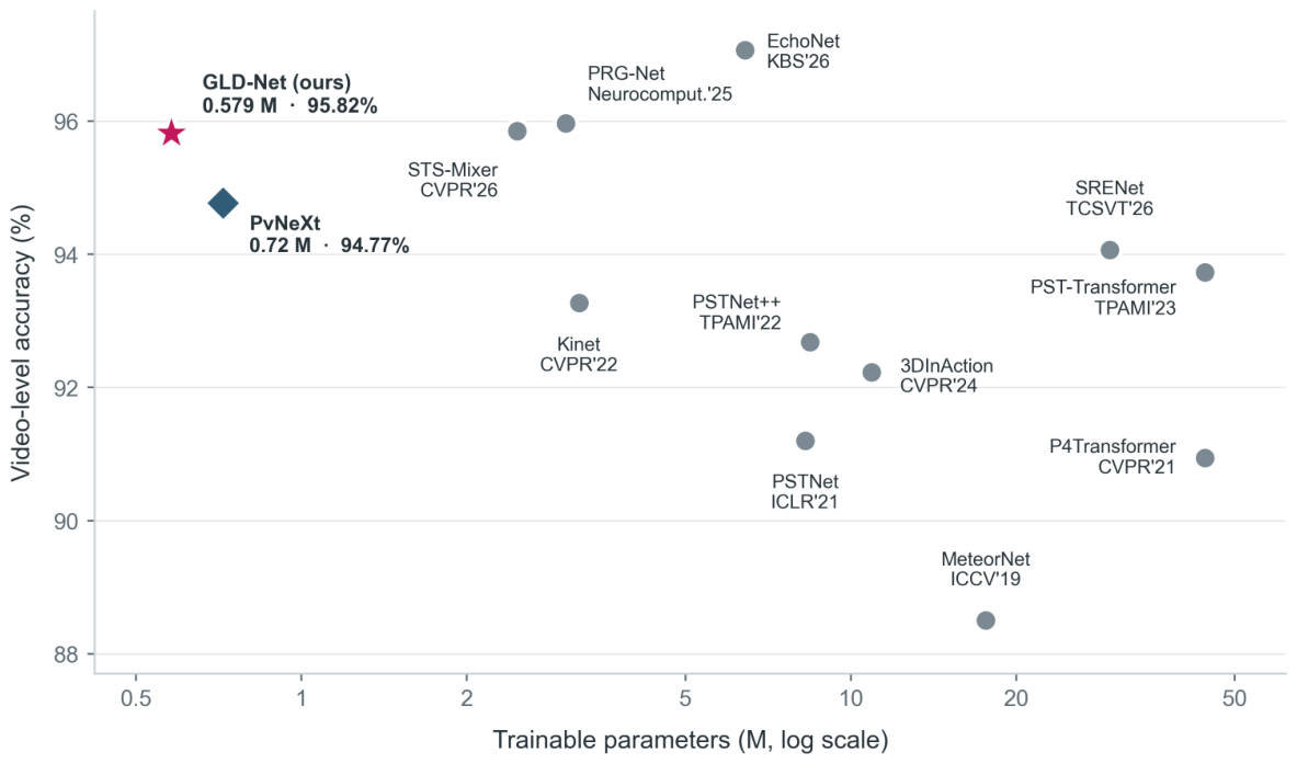
Figure 2.
Overview of GLD-Net. (a) Nearest-neighbor distances to the preceding and succeeding frames are normalized within each frame into motion representations and and then concatenated with three-dimensional coordinates and a normalized temporal feature to form a six-dimensional point descriptor. (b) The global stream and three local streams separately extract frame features and perform bidirectional differencing; they are aggregated into two tokens per frame and then passed to the temporal Transformer.
Figure 2.
Overview of GLD-Net. (a) Nearest-neighbor distances to the preceding and succeeding frames are normalized within each frame into motion representations and and then concatenated with three-dimensional coordinates and a normalized temporal feature to form a six-dimensional point descriptor. (b) The global stream and three local streams separately extract frame features and perform bidirectional differencing; they are aggregated into two tokens per frame and then passed to the temporal Transformer.
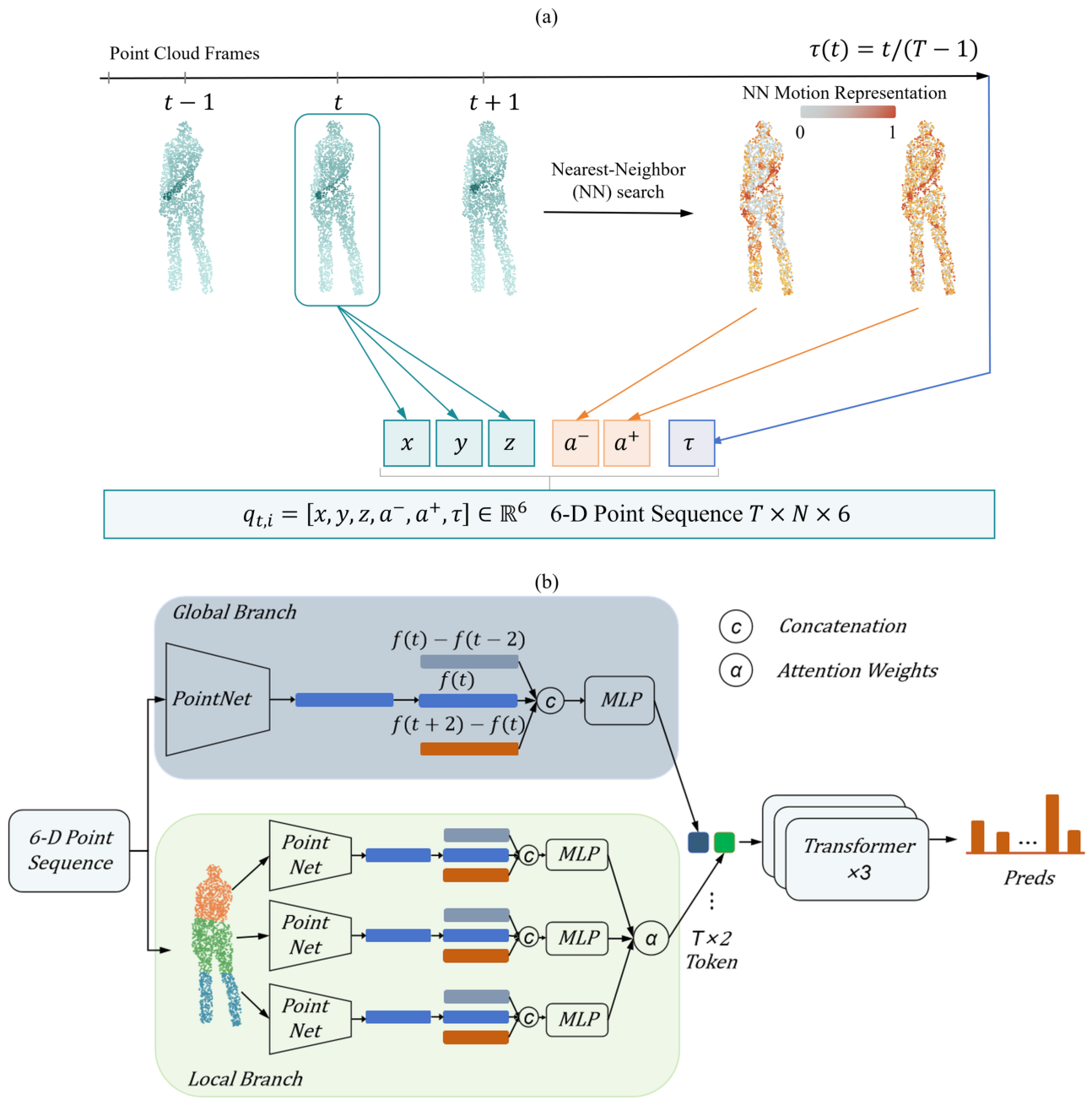
Figure 3.
Computation of the point-level bidirectional nearest-neighbor motion representation. A point in frame t is used as the query point, and its nearest neighbors are searched in the point sets of the preceding frame and succeeding frame . Only the minimum distance in each temporal direction is retained and denoted as the backward distance and forward distance .
Figure 3.
Computation of the point-level bidirectional nearest-neighbor motion representation. A point in frame t is used as the query point, and its nearest neighbors are searched in the point sets of the preceding frame and succeeding frame . Only the minimum distance in each temporal direction is retained and denoted as the backward distance and forward distance .
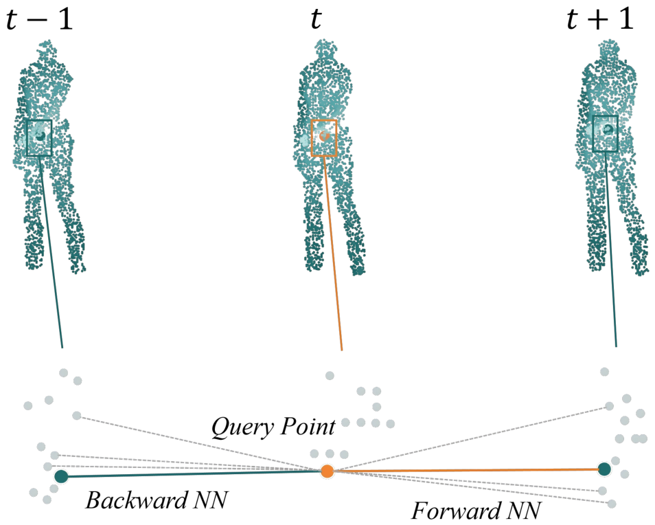
Figure 4.
Feature-level bidirectional differencing (). Each feature stream is subtracted from the corresponding-stream features frames earlier and later. The differences are concatenated with the current feature and mapped back to 128 dimensions. The global stream uses a direct linear mapping, whereas the local streams use a low-rank mapping.
Figure 4.
Feature-level bidirectional differencing (). Each feature stream is subtracted from the corresponding-stream features frames earlier and later. The differences are concatenated with the current feature and mapped back to 128 dimensions. The global stream uses a direct linear mapping, whereas the local streams use a low-rank mapping.
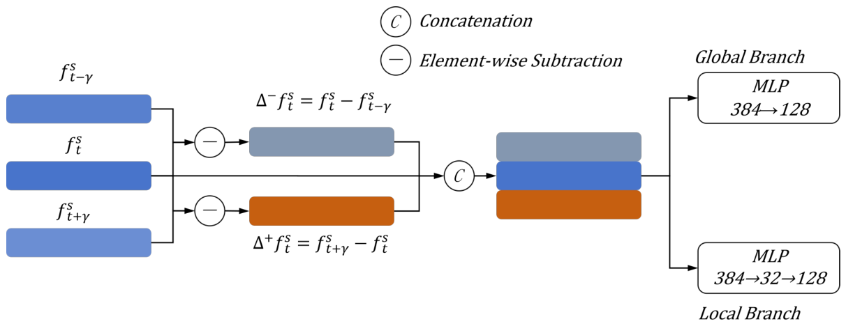
Figure 5.
Execution pipeline of the temporal Transformer. The two tokens in the same frame share a frame-position embedding. After being flattened into 48 tokens, they pass through three pre-normalization encoder layers, and temporal max pooling and a classification head then produce the prediction.
Figure 5.
Execution pipeline of the temporal Transformer. The two tokens in the same frame share a frame-position embedding. After being flattened into 48 tokens, they pass through three pre-normalization encoder layers, and temporal max pooling and a classification head then produce the prediction.
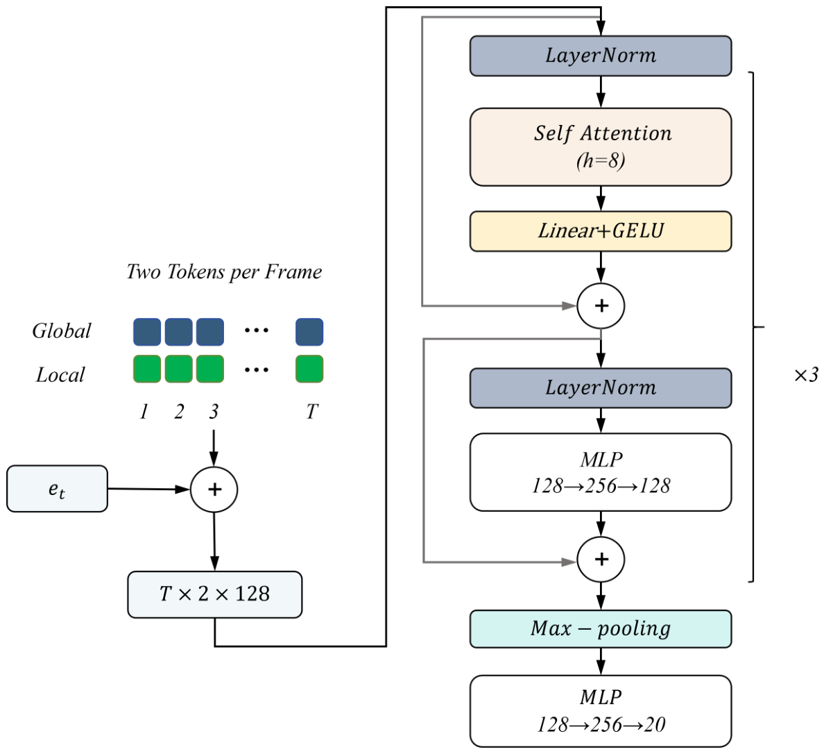
Figure 6.
Point-level visualizations of four actions over five adjacent frames. The upper row shows the nearest-neighbor motion representation from Equation (2), using the same color scheme as Figure 2(a), where warmer colors indicate larger motion. The lower row shows the input points that attain the maximum value in channel-wise max pooling, where warmer colors indicate that a point wins in more channels.
Figure 6.
Point-level visualizations of four actions over five adjacent frames. The upper row shows the nearest-neighbor motion representation from Equation (2), using the same color scheme as Figure 2(a), where warmer colors indicate larger motion. The lower row shows the input points that attain the maximum value in channel-wise max pooling, where warmer colors indicate that a point wins in more channels.
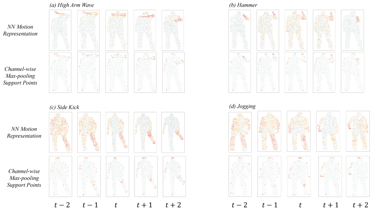

Table 1.
Comparison on MSR-Action3D.
| Method | Source | Parameters (M) | Computation (G) | Accuracy (%) |
|---|---|---|---|---|
| MeteorNet [6] | ICCV 2019 | 17.60 | 1.70 | 88.50 |
| PSTNet [8] | ICLR 2021 | 8.26 | 29.06 | 91.20 |
| P4Transformer [7] | CVPR 2021 | 44.14 | 32.55 | 90.94 |
| PSTNet++ [28] | TPAMI 2022 | 8.43 | 30.21 | 92.68 |
| Kinet [10] | CVPR 2022 | 3.20 | 10.35 | 93.27 |
| PST-Transformer [9] | TPAMI 2023 | 44.13 | 32.56 | 93.73 |
| 3DInAction [29] | CVPR 2024 | 10.90 | – | 92.23 |
| PRG-Net [33] | Neurocomputing 2025 | 3.03 | 8.53 | 95.97 |
| Mamba4D [12] | CVPR 2025 | – | – | 93.38 |
| PvNeXt [11] | ICLR 2025 | 0.72 | 0.55 | 94.77 |
| SRENet [30] | TCSVT 2026 | 29.60 | – | 94.07 |
| STS-Mixer [13] | CVPR Findings 2026 | 2.47 | – | 95.85 |
| EchoNet [34] | KBS 2026 | 6.42 | 7.77 | 97.07 |
| GLD-Net (This work) | This work | 0.579 | 1.42 | 95.82 |
Table 2.
Component ablation on MSR-Action3D.
| NN motion representation | Feature differencing | Global | Local | Temporal Transformer | Accuracy (%) | (pp) |
|---|---|---|---|---|---|---|
| 92.68 | ||||||
| 88.15 | ||||||
| 91.99 | ||||||
| 92.33 | ||||||
| 95.82 | – |
Table 3.
Sensitivity analysis of the number of local segments on MSR-Action3D.
| Number of segments | Parameters (M) | Accuracy (%) |
|---|---|---|
| 2 | 0.557 | 86.76 |
| 3 | 0.579 | 95.82 |
| 4 | 0.601 | 95.47 |
| 5 | 0.623 | 92.68 |
| 6 | 0.645 | 74.22 |
| 7 | 0.667 | 83.62 |
| 8 | 0.689 | 93.03 |
Table 4.
Sensitivity analysis of temporal Transformer depth and number of heads on MSR-Action3D.
| Depth | Heads | Parameters | Accuracy (%) |
|---|---|---|---|
| 1 | 8 | 314,421 | 95.47 |
| 2 | 8 | 446,517 | 94.08 |
| 3 | 8 | 578,613 | 95.82 |
| 4 | 8 | 710,709 | 89.55 |
| 3 | 2 | 578,613 | 91.99 |
| 3 | 4 | 578,613 | 94.77 |
| 3 | 8 | 578,613 | 95.82 |
The four-layer, eight-head row uses a learning rate of 0.001; all other rows use 0.01. All runs are trained for 50 epochs.
Table 5.
Comparison on NTU RGB+D 60 under the cross-subject protocol.
| Method | Source | Parameters (M) | Computation (G) | Accuracy (%) |
|---|---|---|---|---|
| 3DV-Motion [58] | CVPR 2020 | – | – | 84.50 |
| 3DV-PointNet++ [58] | CVPR 2020 | – | – | 88.80 |
| PSTNet [8] | ICLR 2021 | 8.5 | 19.6 | 90.50 |
| P4Transformer [7] | CVPR 2021 | 65.2 | 48.6 | 90.20 |
| PSTNet++ [28] | TPAMI 2022 | – | – | 91.40 |
| PST-Transformer [9] | TPAMI 2023 | 65.2 | 48.6 | 91.00 |
| PvNeXt [11] | ICLR 2025 | 0.9 | 7.8 | 89.20 |
| GLD-Net (masked depth maps) | This work | 2.20 | 3.23 | 83.27 |
| GLD-Net (+ ground removal) | This work | 2.20 | 3.23 | 86.63 |
Disclaimer/Publisher’s Note: The statements, opinions and data contained in all publications are solely those of the individual author(s) and contributor(s) and not of MDPI and/or the editor(s). MDPI and/or the editor(s) disclaim responsibility for any injury to people or property resulting from any ideas, methods, instructions or products referred to in the content. |
© 2026 by the authors. Licensee MDPI, Basel, Switzerland. This article is an open access article distributed under the terms and conditions of the Creative Commons Attribution (CC BY) license.
Copyright: This open access article is published under a Creative Commons CC BY 4.0 license, which permit the free download, distribution, and reuse, provided that the author and preprint are cited in any reuse.