

Submitted:
10 September 2026
Posted:
11 September 2026
You are already at the latest version
Abstract
Explainable AI (XAI) evaluation has matured substantially for static classifiers, yet, to the best of our knowledge, no reproducible benchmark has combined explanation-quality evaluation with the on-device, energy-system-specific setting this paper addresses — smart-grid edge controllers, home and building energy management agents, industrial energy IoT, electric-vehicle charging and vehicle-to-grid systems, and renewable microgrid controllers. ExplainBench evaluates explanation quality within agentic decision workflows; it does not evaluate agent capability, autonomy, or intelligence, and provides no runtime assurance or control function. This paper introduces ExplainBench, the fourth module of the BQEB (BIO-Quantum Energy Brain) research program. Consistent with the architecture established across Papers 1–3, ExplainBench introduces no new architectural layer: it registers as the fourth module of the existing Benchmark Evolution Layer, alongside ForecastBench, SecBench, and FoundationBench, and records the reproducibility metadata, attribution provenance, and human-rating protocols this evaluation requires within the existing Software and Scientific Lineage Layer registries, rather than defining parallel mechanisms. The framework specifies nine component metrics — faithfulness, fidelity, stability, consistency, actionability, uncertainty awareness, human interpretability, computational efficiency, and deployment suitability — formally aggregated into six composite indices: the Explainability Quality Index (EQI), Explanation Stability Score (ESS), Counterfactual Consistency Score (CCS), Energy Decision Transparency Score (EDTS), Human Interpretability Rating (HIR), and Explanation Efficiency Index (EEI), assembled into an Explainability Reliability Matrix across a registry of eight forecasting architectures and eight explanation methods. Six algorithms specify benchmark execution, per-instance metric computation, counterfactual scoring, composite aggregation, cross-model statistical comparison, and leaderboard generation, each with explicit complexity bounds. This manuscript defines benchmark infrastructure; it reports no executed evaluations, and every planned-output table in this manuscript is explicitly marked reserved for future experimental validation, consistent with the evidentiary discipline established in Papers 1–3.
Keywords:
explainable AI
; interpretability benchmarking
; on-device agentic AI
; energy AI
; trustworthy AI
; counterfactual explanation
; faithfulness evaluation
; reproducible benchmarking
1. Introduction
Autonomous, on-device AI agents are increasingly embedded in energy infrastructure: smart-grid edge controllers issuing dispatch-relevant decisions from substation-level telemetry, home and building energy management agents scheduling batteries and HVAC loads, industrial energy IoT systems optimizing plant-level consumption, electric-vehicle charging and vehicle-to-grid (V2G) controllers, and renewable microgrid controllers balancing intermittent generation against demand [1,2]. These systems increasingly rely on foundation-model-based forecasters and learned decision policies whose internal reasoning is not directly inspectable by the grid operators who must act on their outputs [3]. Explainable AI (XAI) offers a partial remedy — attribution methods, counterfactual explanations, and attention-based rationales can, in principle, make a model's reasoning legible to a human operator — but the evaluation of explanation quality itself remains an open, actively contested research problem even for static classifiers [4,5], and, to the best of our knowledge, no reproducible benchmark evaluates explanation quality specifically for the on-device, resource-constrained, safety-relevant setting that energy-system agents occupy.
This gap has a specific, well-documented shape. First, faithfulness metrics — whether an explanation accurately reflects a model's true reasoning — are known to disagree with one another and to lack a reliable ground truth [6,7], a problem compounded rather than resolved when the underlying model is a large pretrained forecaster rather than a small classifier. Second, trust calibration research shows that explanations can as easily produce overtrust as appropriate reliance [8,9], a risk with direct physical consequences when the decision being explained concerns grid dispatch or protective action. Third, existing edge-AI-for-energy reviews treat explainability as a stated requirement rather than a measured property [2,10], leaving a benchmark-shaped gap between the stated need for transparency and any reproducible way to quantify whether a given explanation method satisfies it.
1.1. Relationship to Papers 1–3
ExplainBench introduces no new architectural layer. The governing architecture remains the four-layer design established in Paper 1 — Research Artifact, Reproducibility, Benchmark Evolution, and Scientific Lineage — with SecBench additionally introducing a Threat Layer specific to its own cyber-resilience scope, which this paper does not use or extend. This paper registers within the existing Benchmark Evolution Layer as its fourth module, alongside ForecastBench, SecBench, and FoundationBench. Where this paper's own sections describe a mechanism the companion papers already define — the software registry pattern, the reproducibility guarantees, the governance concordance process — the description is intentionally brief and cites the relevant paper for the complete specification. Within the Benchmark Evolution Layer registry, ExplainBench introduces an explanation-method registry entry type (Section 3); within the existing Scientific Lineage Layer registry, it records benchmark-specific metadata requirements — an attribution-provenance record and a human-rating-consent protocol (Section 6) — that no prior module required, because no prior module evaluated explanations generated for or by a human operator. Neither addition constitutes a governance, authorization, or control mechanism; both are metadata records.
Task scope is deliberately bounded relative to what it could have been. ExplainBench evaluates explanation quality for the forecasting models FoundationBench already registers — Chronos, TimesFM, Moirai, PatchTST, Informer, Autoformer, LSTM, and a standard Transformer baseline — rather than defining a new model registry from scratch. This is a deliberate choice to avoid architectural duplication: the research question this module answers is not “which model forecasts energy load or price best” but “how well can a human operator understand why a given forecast or dispatch-relevant recommendation was produced, and how should that understanding be measured reproducibly.”
2. Related Work
Faithfulness evaluation for post-hoc explanations has developed primarily around perturbation-based protocols: removing or masking the features an explanation marks as important and measuring the resulting change in model output, formalized in comprehensiveness and sufficiency metrics [5] and surveyed extensively for NLP settings [6]. A persistent finding across this literature is that faithfulness metrics frequently disagree with one another across comparative studies [11], motivating the diagnosticity-first framing this paper adopts for its own Faithfulness component (Section 5). Chain-of-thought explanations introduce a distinct faithfulness problem: a model's stated reasoning can diverge from the computation that actually produced its output [12,13], and recent work argues chain-of-thought should not be treated as explainability at all without independent verification [14].
Stability and robustness of explanations — whether small input perturbations produce disproportionately large changes in the explanation itself — were formalized through a Lipschitz-continuity lens [15], which this paper's Stability component (Section 5) adopts directly. Counterfactual explanation, the dominant example-based explanation family, has been reviewed extensively [16,17,18]; the foundational framing treats a counterfactual as the minimal input change that would have altered a decision [19], a framing this paper extends into the Actionability component by additionally requiring that the implied change be operationally feasible for a grid operator to execute, following the algorithmic-recourse literature's own distinction between a valid counterfactual and an actionable one [19].
Trust calibration between human operators and AI systems has been surveyed comprehensively [8], with empirical work showing that displaying model confidence alone does not guarantee appropriate reliance [9] and that cognitive-forcing interventions can reduce but not eliminate overreliance [20]. This literature motivates treating Human Interpretability and Uncertainty Awareness as distinct, separately measured components (Section 5) rather than assuming that any explanation which increases stated trust is thereby a good explanation.
Three prior efforts evaluate explanation quality systematically and are the closest points of comparison for this paper's contribution. M4 evaluates faithfulness metrics for feature-attribution methods across image and text modalities and multiple network architectures within a unified NeurIPS Datasets and Benchmarks framework [21]; ERASER provides a benchmark and metric suite for rationalized NLP models specifically [5]; Quantus is a general-purpose XAI evaluation toolkit covering 35+ metrics across faithfulness, robustness, and complexity, with declared support for time-series data alongside image, tabular, and NLP inputs [36]. None targets energy-system forecasting models specifically, none targets the on-device or edge-deployment setting, and none provides versioned reproducibility infrastructure connecting benchmark artifacts to a broader research architecture; Quantus's own documentation additionally does not provide a mechanism for assessing alignment with human intuition, which this paper's Human Interpretability Rating (Section 5) is designed to measure directly. Table 5 compares all three against ExplainBench across eight dimensions, without asserting superiority beyond what that comparison actually supports: ExplainBench's contribution is not broader modality coverage — all three prior efforts span more models or modalities than this paper's energy-scoped registry — but energy-specific explainability evaluation, time-series forecasting explanation, edge-deployment-constrained metrics, and a reproducibility protocol inherited from a versioned research architecture. Outside explainability specifically, AgentBench's multi-environment, multi-dimensional benchmark configuration methodology [35] is a useful structural precedent for this paper's own Benchmark Configuration Matrix (Table 11), though AgentBench evaluates agentic task success rather than explanation quality and is cited here for its benchmark-construction methodology only, not as a comparable explainability benchmark.
Edge AI for energy systems has been reviewed as an application domain in its own right, with explainability increasingly named as a requirement for operator trust and regulatory compliance in distributed, multi-agent energy management [2,10], though these reviews describe explainability as a design goal rather than measuring it. This paper's contribution is the measurement layer that literature has called for but not yet specified reproducibly.
3. ExplainBench Framework
ExplainBench occupies the existing Benchmark Evolution Layer as its fourth module, shown in Figure 1. It does not modify the Data, Threat, or Reproducibility Layers, and it introduces no governance, authorization, or control mechanism of its own. Within the Benchmark Evolution Layer registry, it introduces an explanation-method registry entry type specific to XAI methods (Section 3.1). Within the existing Scientific Lineage Layer registry, it records benchmark-specific evaluation metadata requirements: an attribution-provenance record and a rater-consent protocol, documenting how each explanation was generated and, where human ratings are collected, under what consent and anonymization protocol (Section 6).
3.1. Explanation-Method Registry
The registry extends the Benchmark Evolution Layer registry pattern FoundationBench established for forecasting models (Paper 3) with a parallel entry type for explanation methods. Each registered method records its taxonomy category (Section 4), applicable model architectures, computational cost class, and whether it produces a deterministic or stochastic explanation given a fixed seed — a distinction that matters directly for the Stability component (Section 5), since a method that is inherently stochastic (e.g., SHAP's sampling-based approximation) requires averaging over repeated runs before a meaningful stability estimate can be computed, while a deterministic method (e.g., Integrated Gradients given a fixed baseline) does not.
3.2. Registered Model and Method Inventory
ExplainBench evaluates explanation quality for the eight forecasting architectures FoundationBench already registers — Chronos [22], TimesFM [23], Moirai [24], PatchTST [25], Informer [26], Autoformer [27], a standard LSTM [28], and a standard Transformer [29] — against eight registered explanation methods spanning five taxonomy categories (Section 4): SHAP [30], LIME [31], Integrated Gradients [32], Grad-CAM where architecture-appropriate [33], counterfactual explanation [19], attention visualization, general feature attribution, and perturbation analysis. Not every method applies to every model: Grad-CAM requires a convolutional or attention map the underlying architecture exposes, and is accordingly restricted in the compatibility matrix (Table 9) rather than forced onto architectures where it would not produce a meaningful explanation.
3.3 Agentic Decision Explanation Boundary
ExplainBench does not benchmark the agent itself. The manuscript's use of “on-device agentic AI” refers to the deployment context this benchmark targets, not to a claim that the framework evaluates autonomous decision-making capability. The relevant pipeline runs from sensor and energy data, through a forecasting foundation model, through a decision agent that consumes that forecast, to a recommended action a human operator ultimately acts on:
| Sensor / Energy Data |
| ↓ |
| Forecasting Foundation Model (registered,Table 2) |
| ↓ |
| Decision Agent |
| ↓ |
| Recommended Action |
| ↓ |
| Human Operator |
ExplainBench evaluates three components of this pipeline: (1) Model Output Explanation — whether the forecasting model's output is faithfully and stably explained (Faithfulness, Fidelity, Stability; Eqs. 1–3); (2) Decision Recommendation Explanation — whether the recommendation derived from that forecast is transparently and actionably explained (Counterfactual Consistency, Actionability, Uncertainty Awareness; Eqs. 4–6); and (3) Human Interpretability — whether a human operator can use the resulting explanation (Eq. 7). The forecasting model is the computational substrate this benchmark's registered explanation methods operate on; the benchmark evaluates explanation quality at the model-output and decision-recommendation boundary, not the decision agent's own internal policy, planning, or reasoning process.
The benchmark does not claim to evaluate autonomous agent intelligence; instead, it evaluates the transparency and interpretability of explanations generated within agentic decision workflows. This scope is deliberate rather than a limitation to be minimized: evaluating decision-agent policy quality is a different research question from evaluating explanation quality, and conflating the two would overstate what this framework measures. In this manuscript, trustworthy refers specifically to reproducible evaluation of explanation quality and human interpretability, not to runtime assurance, autonomous capability assessment, or safety certification.
4. Explainability Taxonomy
ExplainBench organizes registered explanation methods into five taxonomy categories, adapted from established XAI surveys [4,34] to the specific set of methods and architectures this benchmark registers rather than proposed as a general-purpose taxonomy in its own right.
- Attribution-based: assigns an importance score to each input feature or timestep (SHAP, Integrated Gradients, general feature attribution).
- Surrogate-based: fits an interpretable local model and explains via the surrogate (LIME).
- Example-based: explains via a contrastive or counterfactual instance rather than a score (counterfactual explanation).
- Attention-based: explains via the architecture's own internal attention weights, applicable only to attention-bearing models (attention visualization, Grad-CAM where applicable).
- Perturbation-based: explains via systematic input perturbation and output-change observation, used both as a standalone method and as the mechanism underlying the Faithfulness component itself (perturbation analysis).
This taxonomy is deliberately method-oriented rather than output-oriented: two methods in different categories can produce superficially similar visualizations (e.g., both SHAP and an attention map can be rendered as a per-timestep heatmap) while resting on entirely different assumptions about what is being measured, and conflating them would undermine the category-aware compatibility checking Table 9 performs.
5. Mathematical Formulation
Consistent with the formal specification style established across this research program, and building on the explanation notation e = g(x, f) already used throughout this section, ExplainBench is defined as a 5-tuple B = (M, G, D, C, R):
- M — the model registry: the eight registered forecasting architectures (Table 2), reused unmodified from FoundationBench, with no ExplainBench-specific model variant.
- G — the explanation-method registry: the eight registered XAI methods (Table 3), each producing an explanation e = g(x, f) for a given input window x and model f ∈ M.
- D — the dataset: BQEB-Data v1 (Table, Paper 1), reused unmodified, with no ExplainBench-specific dataset variant.
- C — the metric framework: nine component metrics (Section 5.1) aggregated into six composite indices — EQI, ESS, CCS, EDTS, HIR, EEI (Section 5.2) — assembled into the Explainability Reliability Matrix.
- R — the reproducibility artifact set: deterministic-execution records for compatible methods, stochastic run-count and seed-sequence records, human-rater calibration archives, and the evidence-tier classification inherited from the companion architecture paper's Reproducibility Layer (Section 12).
A specific benchmark cell is a tuple (f, φ) ∈ M × G producing an explanation e = φ(x, f), scored under C to yield a component-metric vector and composite-index row of the Explainability Reliability Matrix, with a reproducibility record r ∈ R. No cell of this form has been scored at the time of writing; every symbol above names a specification, not a completed computation.
Let f: X → Y denote a registered forecasting model (Table 2), mapping an input context window x ∈ X to a forecast y-hat = f(x). Let g denote a registered explanation method (Table 3), producing an explanation e = g(x,f) ∈ R^d, a feature- or timestep-level attribution vector over the d inputs unless otherwise specified. Let π denote the ranking of these d features/timesteps induced by e, most-important-first. All notation is used consistently across this section and the algorithms in Section 8.
5.1. Component Metrics
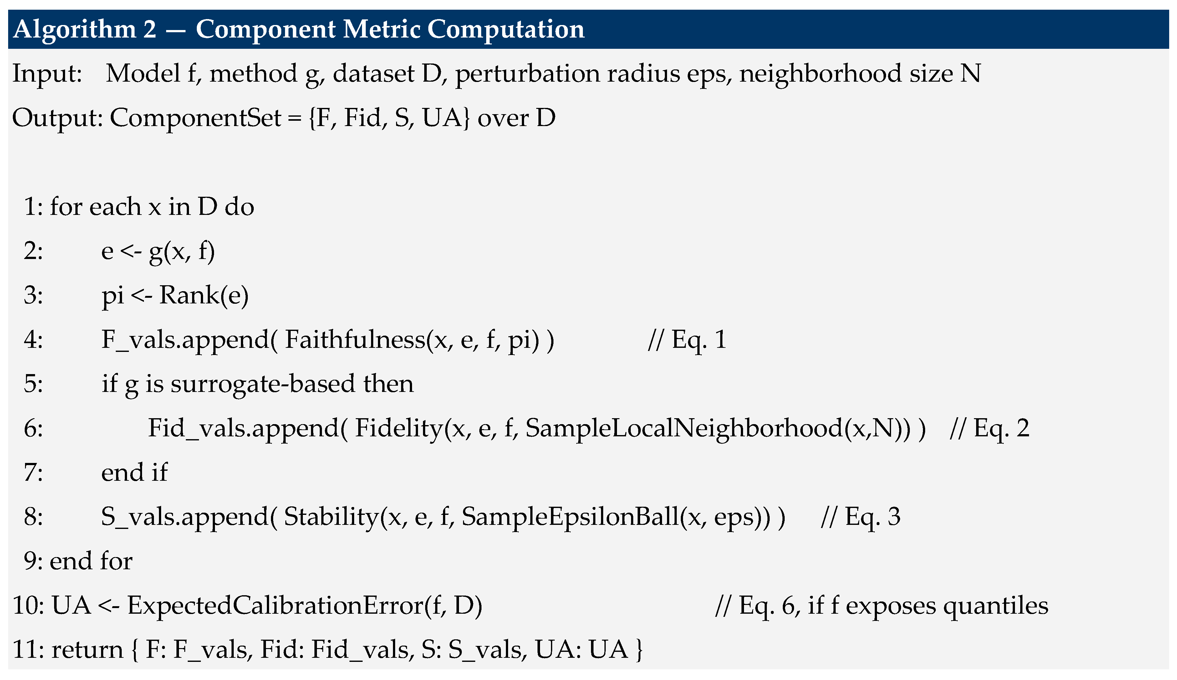
Faithfulness. Following a comprehensiveness-style perturbation protocol [5], the top-k features per π are progressively masked and the resulting change in model output is measured, averaged over k = 1..K and min-max normalized across the registry to [0,1]:
F(x,e,f) = (1/K) * sum_{k=1}^{K} | f(x) - f(x with top-k masked per π) |
Fidelity. Where g induces a local surrogate s_e (e.g., LIME [31]), Fidelity measures agreement between f and s_e over a sampled local neighborhood N(x), distinct from Faithfulness in that it evaluates surrogate agreement rather than reasoning alignment:
Fid(x,e,f) = 1 - (1/|N(x)|) * sum_{x' in N(x)} | f(x') - s_e(x') |
Stability. Following a Lipschitz-continuity formulation [15], explanations should not change disproportionately under small perturbations within an ε-ball B_eps(x):
S(x,e,f) = 1 - max_{x' in B_eps(x)} ( ||e(x)-e(x')||_2 / ||x-x'||_2 )
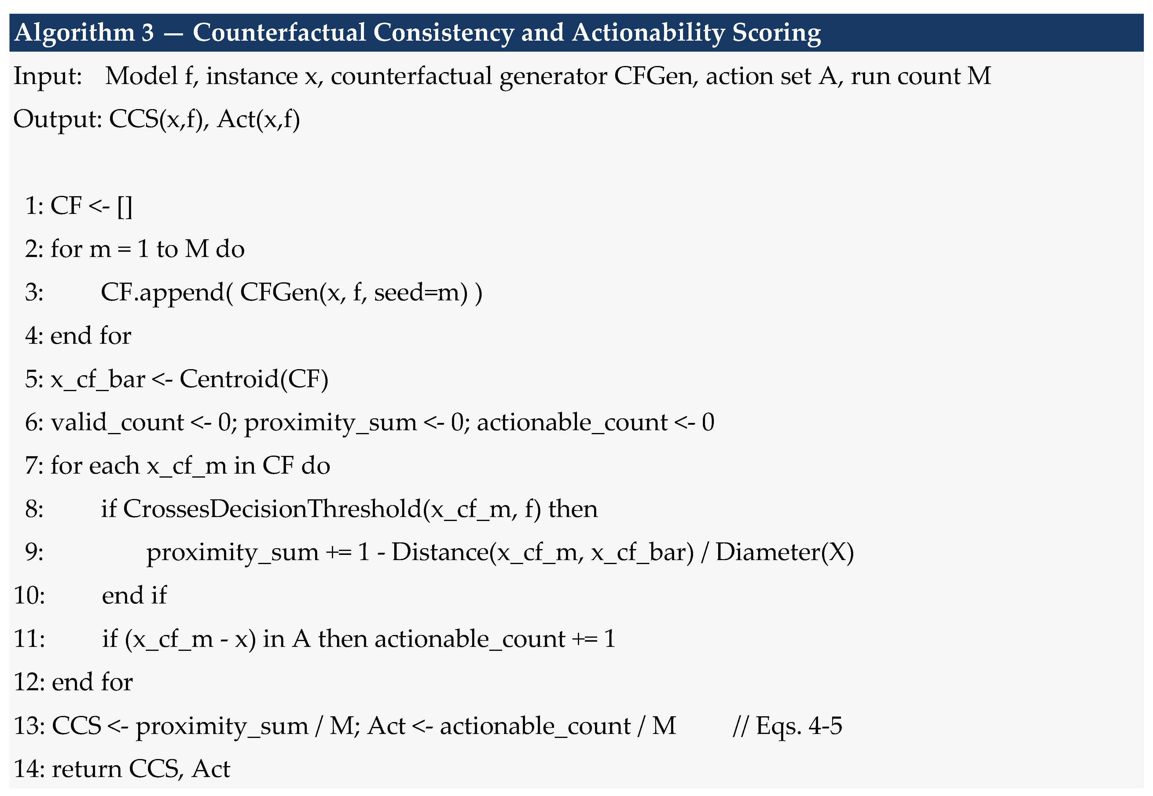
Counterfactual Consistency. Across M independent counterfactual-generation runs (Algorithm 3), validity-weighted proximity to the run centroid x_cf_bar is computed, where validity requires the counterfactual to cross the relevant decision threshold:
CCS(x,f) = (1/M) * sum_{m=1}^{M} 1[valid(x_cf_m)] * (1 - ||x_cf_m - x_cf_bar||_2 / diam(X))
Actionability. Following the algorithmic-recourse framing [19], the fraction of counterfactuals whose implied input change lies within an operationally feasible action set A (i.e., changes a grid operator could actually execute):
Act(x,f) = (1/M) * sum_{m=1}^{M} 1[ (x_cf_m - x) in A ]
Uncertainty Awareness. For models exposing predictive quantiles, measured via Expected Calibration Error across B confidence bins of n_b instances each (N total):
UA(f) = 1 - sum_{b=1}^{B} (n_b/N) * | acc(b) - conf(b) |
Human Interpretability (component). Normalized mean Likert rating across R independent raters (protocol in Section 6.3):
h(e) = (1/R) * sum_{r=1}^{R} (s_r(e) - s_min) / (s_max - s_min)
Computational Efficiency. Latency-normalized against an edge-deployment reference budget t_ref:
Eff(g) = 1 / (1 + t_bar_g / t_ref)
5.2. Composite Indices
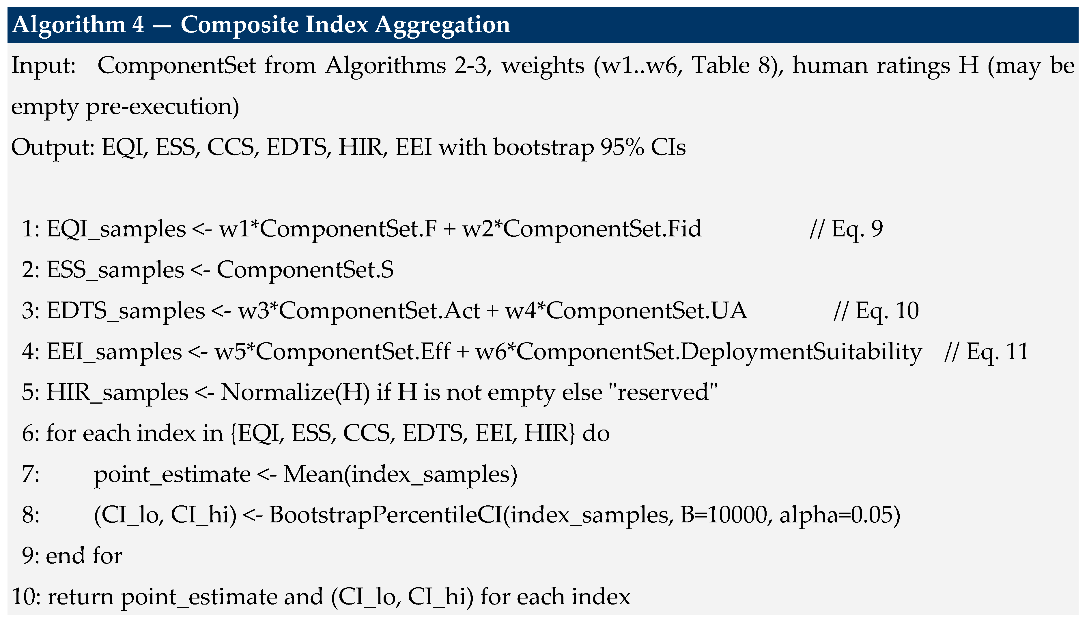
The six composite indices are weighted combinations of the component metrics above, with default equal weighting disclosed as a protocol parameter (Section 6) and sensitivity to alternative weightings reserved for the ablation study (Section 8):
subject to w1+w2=1, w3+w4=1, w5+w6=1. ESS is the evaluation-set mean of S(x,e,f); CCS is already a set-level aggregate (Eq. 4); HIR is the evaluation-set mean of h(e) (Eq. 7). EEI combines computational efficiency and deployment suitability; DeploymentSuitability(g) is formalized as DSS(g) in Section 5.4 (Eq. 12) rather than left qualitative. The Explainability Reliability Matrix R (dimensions M x 6) collects [EQI, ESS, CCS, EDTS, HIR, EEI] for each of the M registered (model, method) pairs and is the tabular structure underlying the radar and leaderboard views (Figure 2); it is not a distinct statistic beyond its constituent columns.
EQI(x,e,f) = w1 * F(x,e,f) + w2 * Fid(x,e,f)
EDTS(x,f) = w3 * Act(x,f) + w4 * UA(f)
EEI(g) = w5 * Eff(g) + w6 * DeploymentSuitability(g)
Assumption. Eqs. (9)–(11) assume the underlying component metrics are independently estimable for a given (model, method, instance) triple; where a method is architecture-incompatible (Table 9), the corresponding row is omitted from R rather than imputed, consistent with the missing-data handling in Algorithm 1.
5.3. Composite Index Design Rationale
Table 4a states the rationale behind each composite index's component grouping explicitly, since a reviewer's first question about any composite metric is reasonably why its components were grouped as they were rather than differently. The six indices are not intended as a universal scoring standard; they provide a structured decomposition of distinct explainability evaluation dimensions.
Equal weighting (w1–w6, Table 8) is selected as a neutral benchmark default, not as an optimized scoring strategy. This paper does not claim equal weighting is the correct weighting for every deployment context; it claims equal weighting is a defensible, disclosed, and reproducible starting point that does not silently favor one component over another. Alternative weighting schemes are explicitly out of scope for this manuscript but are identified as future extensions: expert-elicited weighting, Delphi-method consensus weighting, regulatory-mandated weighting where a jurisdiction specifies minimum transparency requirements, and domain-specific weighting tuned to a particular deployment context (e.g., weighting Actionability more heavily for direct-dispatch agents than for advisory-only agents).
5.4. Deployment Suitability Score (DSS)
Deployment Suitability appears in Table 4 as a component feeding EEI (Eq. 11) but was left qualitative in the original formulation. This subsection formalizes it. Let hardware compatibility, memory efficiency, latency suitability, energy-consumption efficiency, and privacy deployment suitability each be normalized to [0,1] (Table 4b); DSS is their weighted sum:
DSS(g) = u1*HardwareCompat(g) + u2*MemoryEff(g) + u3*LatencySuit(g) + u4*EnergyEff(g) + u5*PrivacySuit(g) (12)
subject to u1+u2+u3+u4+u5=1, with default equal weighting following the same neutral-default rationale as Section 5.3. DSS(g) replaces the qualitative “Deployment Suitability” term in Eq. 11 without otherwise modifying that equation.
6. Benchmark Protocol
This section specifies the dataset scope, benchmark tasks, and protocol parameters that instantiate the mathematical framework of Section 5 into a runnable evaluation, consistent with the same evidentiary discipline established in Papers 1–3: every parameter is disclosed as a design choice, not fitted post hoc against results that do not yet exist.
6.1. Dataset Construction
ExplainBench requires no new dataset. It reuses BQEB-Data v1 exactly as Paper 1 validated it and as FoundationBench scoped it for forecasting evaluation: 10,512 records at 15-minute resolution, with load_mw and energy_price_usd_mwh as the explained targets. What explainability evaluation adds beyond forecasting evaluation is a context-window sampling requirement: explanation quality is evaluated over a stratified sample of windows spanning distinct operating regimes — peak load, off-peak, and ramp periods — rather than a single contiguous test split, since an explanation method's faithfulness and stability can vary systematically across regimes that a single split would not surface (Table 6).
6.2. Benchmark Tasks
Three tasks are defined. Task 1 evaluates explanation quality for next-hour load forecasting; Task 2 evaluates explanation quality for day-ahead price forecasting — both reusing ForecastBench's and FoundationBench's existing targets rather than defining new ones. Task 3 evaluates explanation quality specifically for the six energy-domain deployment contexts (Table 6: smart-grid edge agents, home and building energy management, industrial energy IoT, EV charging/V2G, and renewable microgrid controllers), holding the underlying model and method fixed while varying the deployment context to isolate domain-specific effects on Actionability and Deployment Suitability (Eqs. 5, 8) from effects attributable to the model or method alone.

Table 7.
a. Formal task specification for T1–T3, following the B = (M, G, D, C, R) definition above and supplementing Table 7's overview.
Table 7.
a. Formal task specification for T1–T3, following the B = (M, G, D, C, R) definition above and supplementing Table 7's overview.
| Task | Inputs | Outputs | Labels | Required Artifacts | Assumptions | Success Criteria | Metrics Used |
| T1 | Input window x; registered model f; registered method φ | Explanation e = φ(x,f) for next-hour load forecast | None (unsupervised metric scoring, not classification) | Explanation artifact; run manifest (seed/count for stochastic methods) | Model and method drawn only from Table 2 and Table 3; no gradient update on BQEB-Data v1 | All nine component metrics computed without error for the (f,φ) pair | EQI, ESS, CCS, EDTS (component metrics, Section 5.1) |
| T2 | Input window x; registered model f; registered method φ | Explanation e = φ(x,f) for day-ahead price forecast | None (unsupervised metric scoring) | Explanation artifact; run manifest | Same constraints as T1, applied to the price target | Same as T1, applied to the price target | Same composite set as T1 |
| T3 | T1/T2 output held fixed; varying deployment context (Table 6) | Per-domain Actionability and Deployment Suitability scores | Deployment-context label (one of six, Table 6) | Per-domain explanation artifact; context label record | Model and method held fixed across domains to isolate context effects | Domain-specific EDTS variance attributable to context, not model/method drift | EDTS, HIR (Eqs. 5, 7, 8) |
6.3. Human Interpretability Panel Protocol
Human Interpretability Rating (Eq. 7) requires an independent rater panel, specified here rather than left implicit. Raters are drawn from individuals with domain-relevant grid-operations familiarity, calibrated against a fixed anchor set of example explanations before rating the evaluation set, and rate on a 5-point Likert scale (Table 14) covering clarity, sufficiency, and actionability of the explanation as presented, not the correctness of the underlying forecast. Rater identity is decoupled from the (model, method) pair under evaluation to avoid a rater's prior familiarity with a specific vendor's output biasing the rating, and inter-rater agreement is reported via Krippendorff's alpha rather than assumed.
6.4. Protocol Parameters
Table 8 discloses every free parameter of the protocol — perturbation radius ε, local-neighborhood sample size for Fidelity, bootstrap resample count, counterfactual run count M, and the default composite weights w1–w6 — as fixed, versioned protocol constants rather than values tuned against outcomes, consistent with the reproducibility discipline Section 12 inherits from Paper 1.
Table 2 lists the eight registered forecasting models, reused from FoundationBench's registry (Paper 3) rather than newly specified.
Table 5 compares ExplainBench against the three directly comparable prior efforts identified above, across the dimensions most relevant to an energy-domain, on-device explainability benchmark.
Table 6 lists the six energy-domain deployment contexts Task 3 (Section 6.2) evaluates against.
Table 7 summarizes the three benchmark tasks defined in Section 6.2.
Table 8 discloses every free parameter of the evaluation protocol as a fixed, versioned constant.
7. Explainability Metrics
Section 5 defines every metric mathematically; this section addresses how those definitions are operationalized across the registry. Figure 2 shows the resulting hierarchy: nine component metrics feed six composite indices, which are in turn assembled into the Explainability Reliability Matrix (Section 5.2) and evaluated against the eight registered explanation methods (Table 3).
Two operational distinctions matter beyond the equations themselves. First, not every component applies to every (model, method) pair: Fidelity (Eq. 2) is defined only where the explanation method induces a local surrogate, and is reported as not applicable rather than imputed for methods that do not (Table 3's determinism column flags this alongside the related stochasticity distinction). Second, Uncertainty Awareness (Eq. 6) requires the underlying model to expose predictive quantiles; Chronos, TimesFM, and Moirai do so natively, while the remaining five registered models require a calibration wrapper whose own reproducibility is disclosed in Section 12 rather than assumed.
Table 10 enumerates the failure modes this metric set is designed to surface — an explanation can fail along any one dimension while scoring well on others, and a single Overall Explainability Score would obscure exactly the distinction this benchmark exists to make.
8. Experimental Methodology
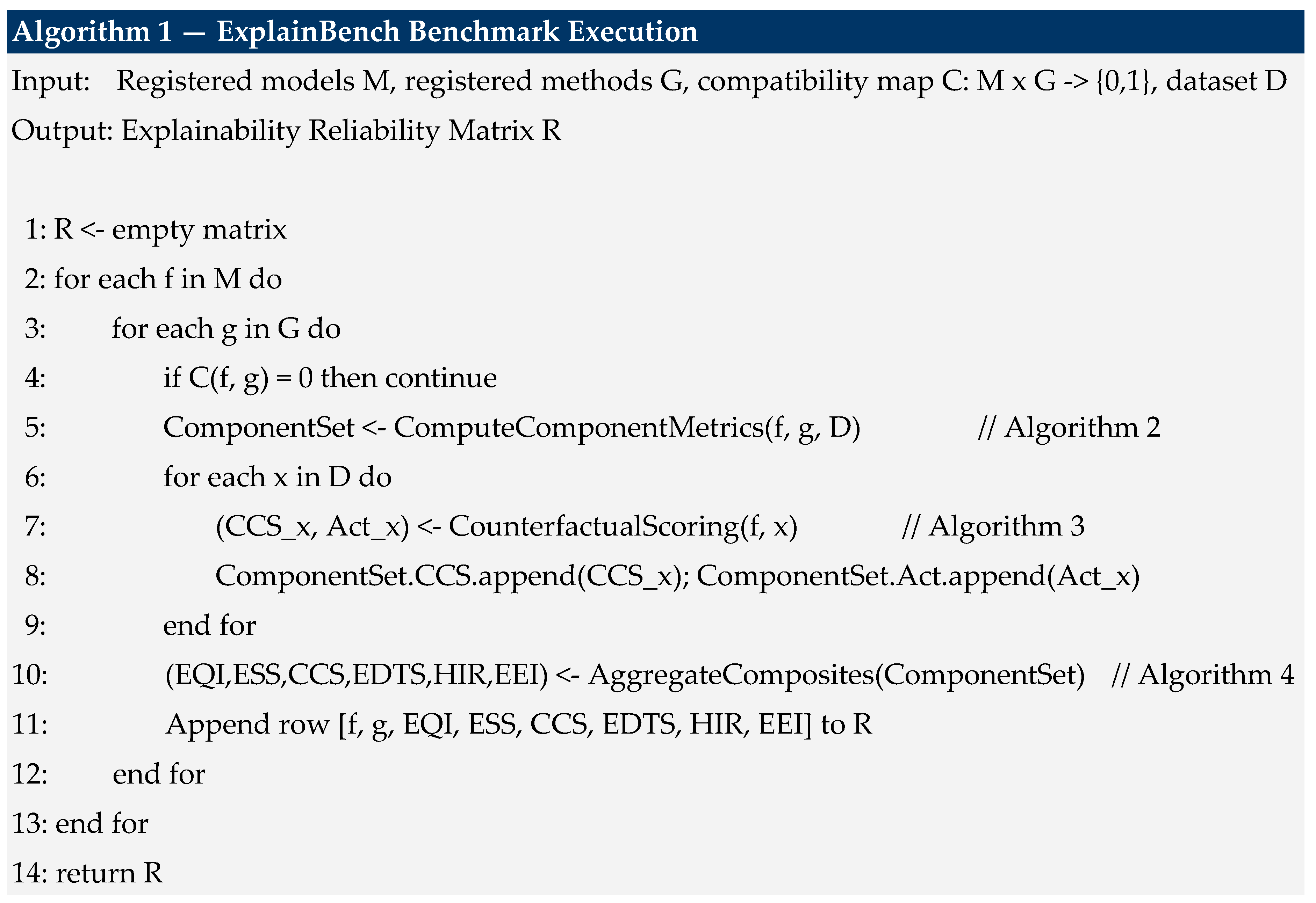
This section specifies the six algorithms that implement the benchmark protocol (Section 6) and metric definitions (Section 5) as a reproducible, executable procedure. Each algorithm is fully specified independent of whether it has been executed; Section 9 discloses execution status explicitly rather than allowing it to be inferred.
8.1. Algorithm 1: Benchmark Execution
Top-level orchestration across the registered model set M (Table 2) and method set G (Table 3), respecting the compatibility map of Table 9.
8.2. Algorithm 2: Component Metric Computation
8.3. Algorithm 3: Counterfactual Scoring
8.4. Algorithm 4: Composite Index Aggregation
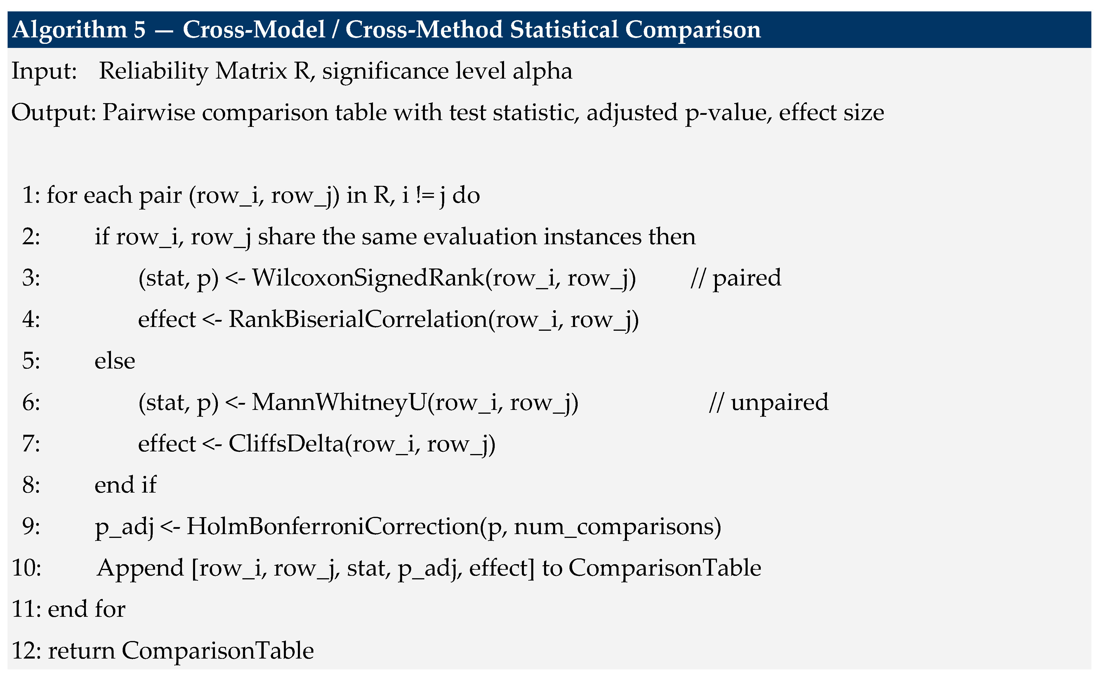
8.5. Algorithm 5: Cross-Model Statistical Comparison
8.6. Algorithm 6: Leaderboard Generation
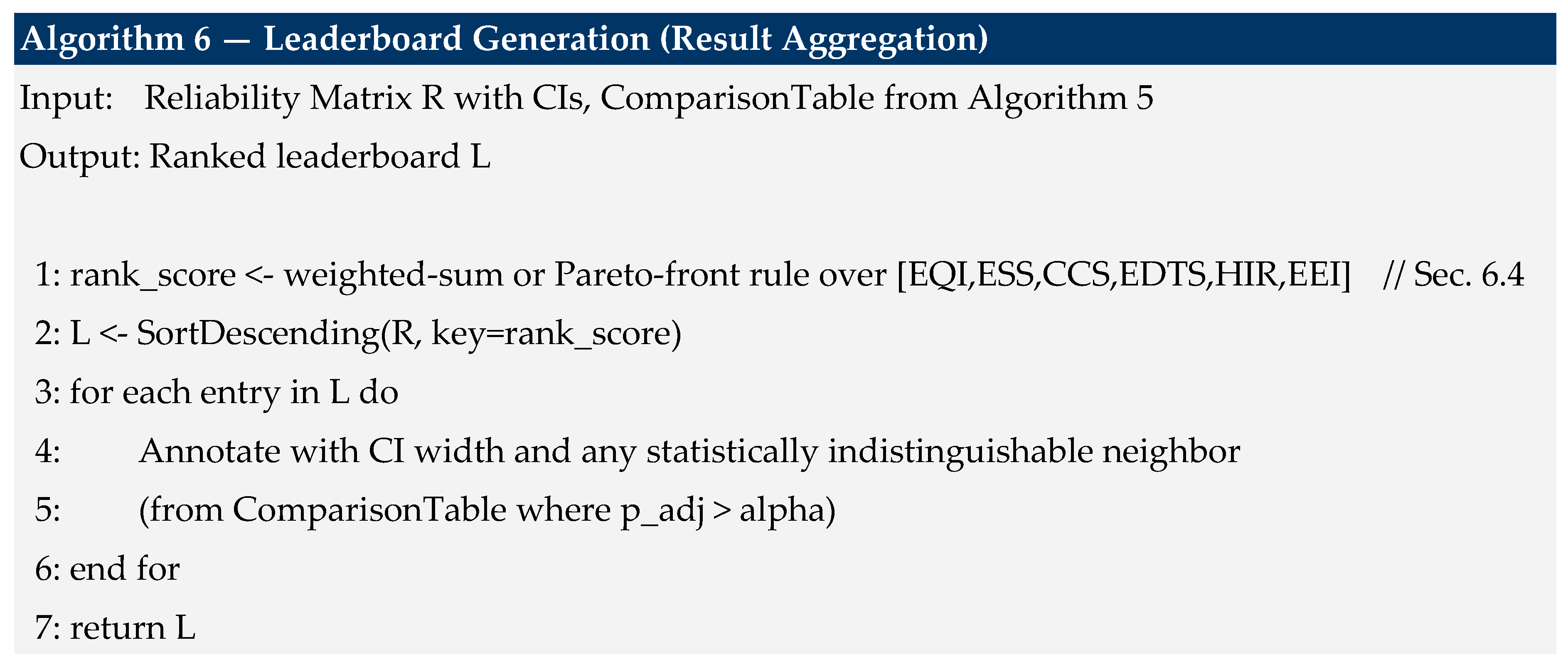
Ties are broken by confidence-interval overlap rather than point-estimate ordering alone: an entry statistically indistinguishable from the entry above it is flagged as co-ranked rather than silently ordered by a non-significant difference, consistent with the statistical treatment specified in Section 8.7.
8.7. Statistical Treatment
Every composite index is reported with bootstrap percentile confidence intervals (B = 10,000 resamples, Algorithm 4). Paired comparisons between models or methods evaluated on the same instances use the Wilcoxon signed-rank test; unpaired comparisons across deployment-mode strata use the Mann-Whitney U test — both non-parametric, appropriate given no assumption of normality for bounded [0,1] indices. Effect size is reported via rank-biserial correlation for paired comparisons and Cliff's delta for unpaired comparisons. Where three or more independent groups are compared and normality and homogeneity of variance are not violated, ANOVA with Games-Howell post hoc testing is used; Kruskal-Wallis is substituted otherwise. All p-values undergo Holm-Bonferroni correction for the number of pairwise comparisons performed (Algorithm 5).
8.8. Ablation Plan
Two ablations are specified, neither executed in this manuscript. The first varies the composite weights (w1–w6, Table 8) away from their default equal-weighting to test whether the resulting leaderboard ranking (Algorithm 6) is sensitive to this disclosed protocol choice. The second removes one component metric at a time from each composite index to test whether any single component dominates its composite's variance, which would indicate the composite is not meaningfully aggregating independent information. Both ablations reuse Algorithm 4, Algorithm 5 and Algorithm 6 unchanged, varying only their inputs.
9. Results and Analysis
Results Pending Experimental Execution
No forecasting model has been evaluated against any registered explanation method under this protocol at the time of writing. This section is deliberately not titled to imply findings: it reports execution status, not results. Table 11 (Benchmark Configuration Matrix) enumerates every registered (model, method) combination this protocol specifies; Table 12 is provided in the exact structure a completed benchmark run will populate.
Cross-domain evaluation (Task 3, Section 6.2) is likewise unexecuted. The protocol requires evaluating the same (model, method) pair across all six energy domains (Table 6) to isolate domain-specific effects on Actionability and Deployment Suitability; the resulting per-domain breakdown is reserved for the same future experimental execution as the primary leaderboard.
Figure 3.
ExplainBench benchmark workflow: end-to-end sequence from model/method registration through the Explainability Reliability Matrix, with results reserved for future experimental execution.
Figure 3.
ExplainBench benchmark workflow: end-to-end sequence from model/method registration through the Explainability Reliability Matrix, with results reserved for future experimental execution.
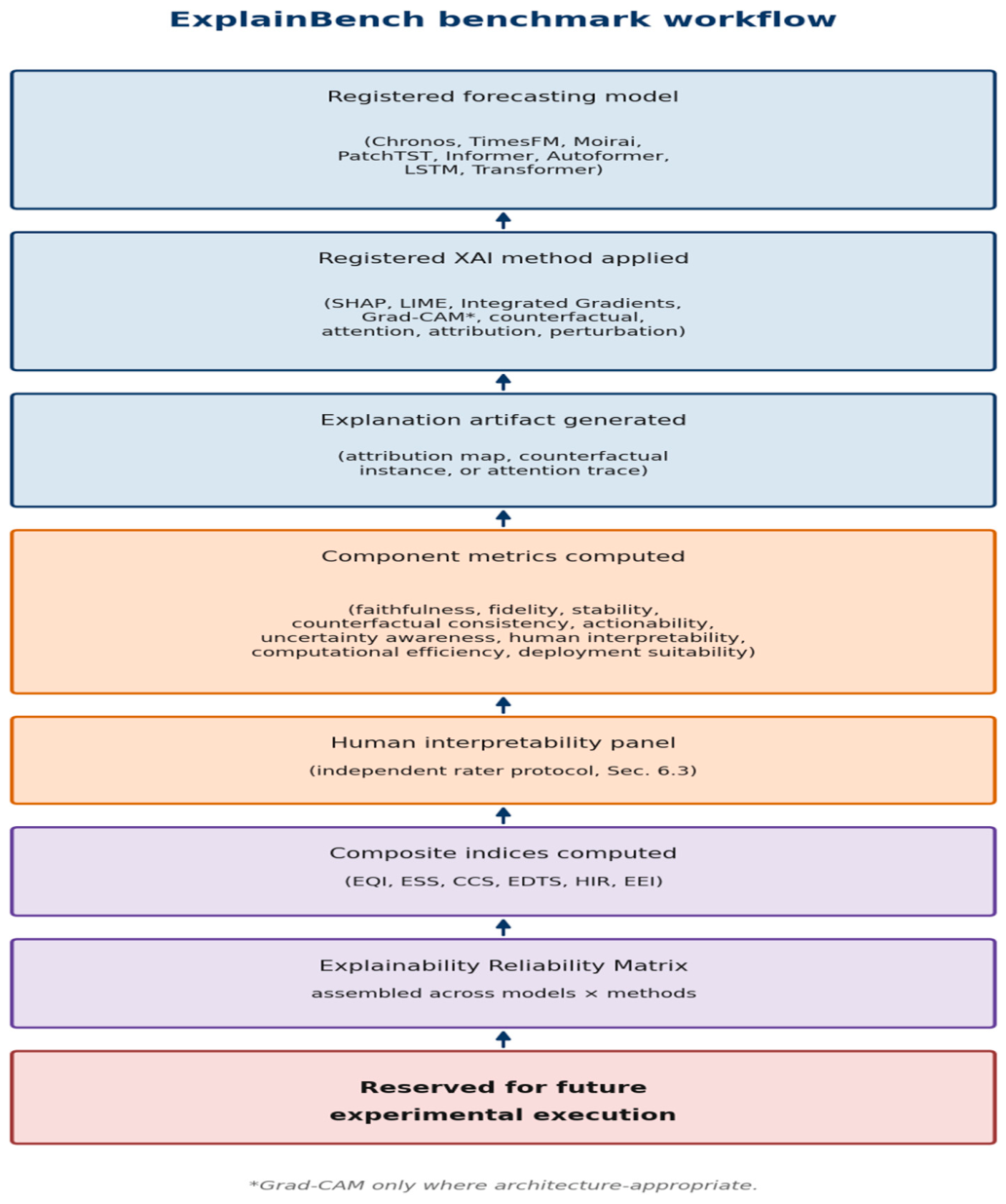
Figure 4.
Per-instance evaluation pipeline, visualizing Algorithm 2 and Algorithm 3: attribution-based component metrics (top) and counterfactual-based component metrics (bottom) converge on Algorithm 4's weighted aggregation.
Figure 4.
Per-instance evaluation pipeline, visualizing Algorithm 2 and Algorithm 3: attribution-based component metrics (top) and counterfactual-based component metrics (bottom) converge on Algorithm 4's weighted aggregation.
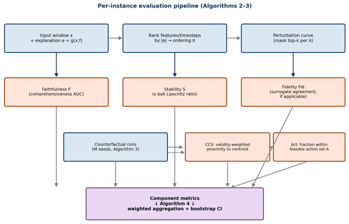
Figure 5.
Explainability Reliability Matrix radar output template. Both traces are flat illustrative placeholders, not measured scores; actual per-method radar profiles are reserved for future experimental execution.
Figure 5.
Explainability Reliability Matrix radar output template. Both traces are flat illustrative placeholders, not measured scores; actual per-method radar profiles are reserved for future experimental execution.
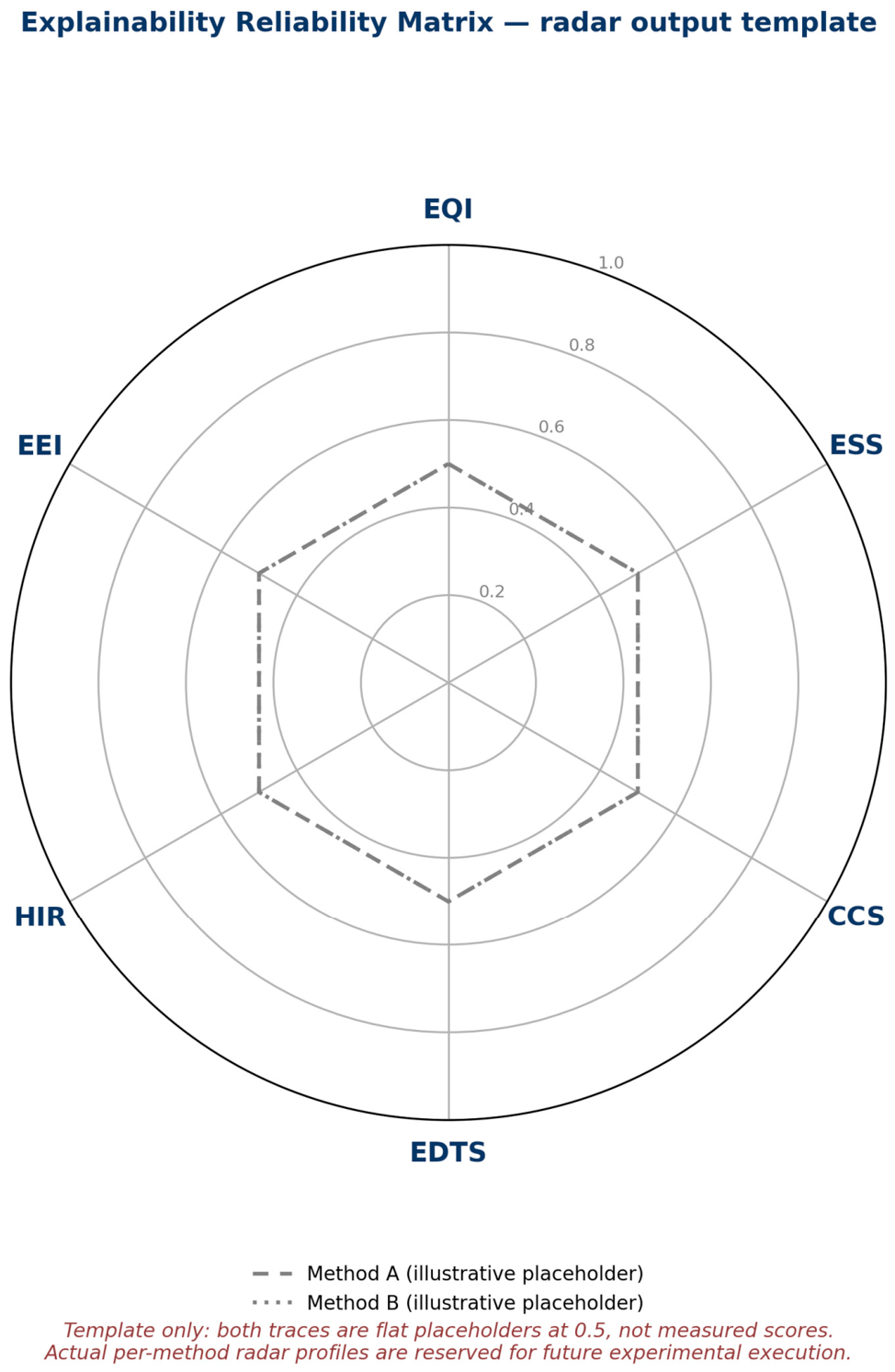
Table 11 enumerates the full registered configuration space: 8 models x 8 methods, restricted by the compatibility map (Table 9), x 6 energy domains (Table 6) for Task 3 specifically.
Table 12 is the reporting template every completed evaluation cell will populate, shown here for the Chronos row across all eight registered methods as a representative excerpt rather than all 58 valid pairs.
10. Discussion
ExplainBench's contribution at this stage is benchmark infrastructure — a registry that distinguishes deterministic from stochastic explanation methods, a metric set that keeps nine independently-diagnosable failure modes (Table 10) separate rather than collapsing them into one score, and a protocol that discloses every free parameter (Table 8) as a versioned constant — not a demonstrated finding about which explanation method is best for which forecasting model. That question is exactly what Section 9 defers to a companion execution study. The design choice most likely to be scrutinized is the decision to include both deterministic and stochastic explanation methods in the same registry rather than restricting to one class; Section 3.1's position is that this heterogeneity reflects the real, current state of the XAI method landscape, and excluding stochastic methods would not make that heterogeneity disappear from a practitioner's actual choice set.
A second design choice worth surfacing explicitly: Actionability (Eq. 5) and Uncertainty Awareness (Eq. 6) are folded into a single composite, EDTS, on the premise that a grid operator's practical need for transparency is jointly about “can I act on this” and “how confident should I be,” rather than two separable concerns. An alternative design would keep these as two separate composites; Table 8's disclosed weighting (w3, w4) makes this choice inspectable and reversible by a downstream user of the protocol, rather than baking the combination in without recourse.
Generalizability Beyond the Current Registry
This specification is written against the eight forecasting models and eight XAI methods currently registered (Table 2 and Table 3), and that dependency should be stated rather than left implicit. Extending ExplainBench to a future explanation method or forecasting architecture requires no new mechanism: a new method registers in the explanation-method registry (Section 3.1) with the same deployment classification (deterministic or stochastic) Table 3 already requires, and the compatibility map (Table 9) is extended, not replaced, since nothing in the component-metric definitions (Section 5.1) assumes a fixed method count. A new agent architecture — for instance, a multi-agent dispatch controller rather than a single-model forecaster — would require the Agentic Decision Explanation Boundary (Section 3.3) to be re-examined, since that boundary is currently scoped to single-model attribution; this is disclosed as a real limit on the framework's current reach, not a claim that the boundary already generalizes to multi-agent settings.
Backward compatibility follows the same registry discipline as FoundationBench: adding a method or model does not retroactively alter how a previously scored cell of the Explainability Reliability Matrix is interpreted, since each cell's deployment mode and seed record are fixed at registration time. Governance of this evolution is inherited from the companion architecture paper's Scientific Lineage Layer rather than redefined here — the same n=1-style boundary the architecture paper discloses for its own extensibility claim applies to this registry too: the mechanism is specified and has processed eight models and eight methods by this program's own registration, but has not yet been exercised by an independent party registering a ninth. Closing that gap is future work, not a claim this manuscript makes about itself.
11. Threats to Validity
- Synthetic data. Every ExplainBench task inherits BQEB-Data v1's synthetic-generation status; explanation quality measured on this benchmark is a statement about explaining a simulator's behavior, not a validated statement about explaining real utility telemetry.
- No ground-truth explanations. Consistent with the broader XAI faithfulness literature [7], none of the component metrics assume access to a ground-truth explanation; Faithfulness and Fidelity are proxies, not direct measurements of a model's true internal reasoning.
- Human panel size and composition. HIR's validity depends on rater panel size and domain-relevant expertise (Section 6.3); a small or non-representative panel would limit how far HIR generalizes beyond the specific raters used.
- Composite weight sensitivity. Default equal weighting (Table 8) is a disclosed but not empirically validated choice; the ablation plan (Section 8.8) is specified but not yet executed, so weight sensitivity itself remains an open question this manuscript does not resolve.
- Single dataset, single simulated region. No cross-dataset or cross-utility validation exists yet for this benchmark.
- Calibration wrapper dependency. Uncertainty Awareness (Eq. 6) for the five models that do not natively expose quantiles depends on a calibration wrapper whose own reliability is a threat this manuscript does not independently validate.
- Deployment scope. ExplainBench evaluates explanation quality only; it provides no runtime assurance, control function, or safety certification, and a high score on this benchmark is not evidence that an explanation is safe to act on in a live dispatch decision.
- Registry extensibility validated at the scale registered here, not beyond it. The explanation-method and model registries have processed exactly the counts this program itself registered (eight methods, eight models); no genuinely independent third-party registration has occurred, the same evidentiary boundary the companion architecture paper discloses for its own extensibility claim.
12. Reproducibility
Deterministic-execution, partitioning, artifact-checksumming, and dependency/environment-pinning mechanisms — including the hash-pinned requirement set the architecture paper verifies in a clean environment — are inherited unchanged from Papers 1–3 for every component that does not involve human rating or stochastic explanation generation. Two extensions are specific to this module. First, stochastic explanation methods (SHAP, LIME, counterfactual search; Table 3) require the number of repeated runs and the random seed sequence to be recorded alongside any reported score, since a single run of a stochastic method is not independently reproducible without that record. Second, human interpretability ratings (Section 6.3) require the rater panel's calibration-set responses to be archived alongside the reported HIR score, so that a future re-rating can be checked for calibration drift rather than assumed consistent.
Table 13 provides the reproducibility checklist for this module, following the same format as Papers 1–3's own checklists.
12.1. Pilot Validation Protocol
No experimental results are reported in this manuscript. This section defines a reproducible validation protocol for future execution, scoped intentionally narrower than the full registry (Table 2 and Table 3) to serve as a minimal, tractable first execution rather than the complete benchmark run Section 9 describes. Table 12a summarizes the pilot scope at a glance before the detailed reporting template (Table 13a) that follows.
The pilot is scoped to two registered models — LSTM and a standard Transformer-based forecaster — evaluated against three registered explanation methods — SHAP, Integrated Gradients, and LIME — on BQEB-Data v1, following the identical dataset construction, task definitions, and protocol parameters specified in Section 6. This subset is chosen because it spans both a deterministic method (Integrated Gradients) and two stochastic methods (SHAP, LIME; Table 3), and because LSTM and Transformer are the two registered architectures with the fewest method-compatibility exclusions (Table 9), minimizing confounds from architecture-specific method restrictions in a first pilot.
The pilot reports five of the six composite indices — EQI, ESS, CCS, HIR, and EEI — using Algorithm 1, Algorithm 2, Algorithm 3 and Algorithm 4 unmodified. EDTS and deployment-context evaluation are reserved for expanded validation because they require domain-specific operational studies — the Task 3 cross-domain protocol (Section 6.2) and the Actionability action-set definition (Eq. 5) — beyond the scope of this initial benchmark pilot; a pilot claiming an EDTS value without executing Task 3 would misrepresent what the pilot actually measured. This exclusion is a deliberate scope boundary of the pilot specifically, not a change to the six-composite framework Section 5.1, Section 5.2, Section 5.3 and Section 5.4 define.
The purpose of this protocol is threefold: to demonstrate that the benchmark as specified is executable end-to-end rather than only theoretically defined; to provide the minimal artifact set (registered models, registered methods, fixed dataset, disclosed protocol parameters) a future replication would need; and to establish a standardized reporting format — Table 13a — that any future execution, pilot or full-scale, populates identically. This protocol does not itself constitute validation of the framework's scientific claims; it is the minimum reproducible procedure by which such validation could later be attempted.
13. Future Work
- Execution of the experimental plan in Section 8, producing the first real results for this benchmark.
- Execution of the ablation plan (Section 8.8): weight sensitivity and component-removal analysis.
- Validation against real or semi-real utility telemetry, where access constraints permit, to test generalization beyond the synthetic simulator.
- Extension of the registry to additional XAI methods as they are published, following the same taxonomy-category and compatibility-map discipline established here (Section 3.1, Table 9).
- Longitudinal human-rater studies to test whether HIR (Eq. 7) is stable over time for the same explanation, distinct from the single-session calibration this protocol currently specifies.
14. Conclusion
This paper has specified ExplainBench, the fourth module of the BQEB Benchmark Evolution Layer, extending the existing four-layer architecture with an explanation-method registry and a nine-component, six-composite evaluation framework for on-device agentic AI in energy systems. Three benchmark tasks, a full mathematical formulation (Section 5), six algorithms (Section 8), and a reproducibility extension recording the required Scientific Lineage Layer metadata (Section 12) are fully specified. No results are reported: Section 9 marks them explicitly reserved for future experimental execution, and this disclosure is treated as part of the contribution rather than a gap to be minimized. ExplainBench extends the BQEB Benchmark Evolution Layer, following ForecastBench, SecBench, and FoundationBench; subsequent modules are named in the program's broader roadmap but not yet scoped.
Author Contributions
Rakesh Kumar Agrawal: Conceptualization, Methodology, Software, Investigation, Writing – Original Draft, Writing – Review & Editing, Visualization.
Funding
No external funding was received for this research.
Data Availability Statement
BQEB-Data v1 is available via Harvard Dataverse (DOI 10.7910/DVN/VUVTED) and IEEE DataPort (DOI 10.21227/xj9b-2885), as established in Paper 1.
Code Availability Statement: ExplainBench is planned to extend the ForecastBench software package (MIT license, Zenodo DOI 10.5281/zenodo.21735978); no ExplainBench-specific software release exists at the time of writing. Registered XAI method implementations are available from their respective publishers' repositories as cited in the References.
Conflicts of Interest
The authors declare no conflict of interest.
References
- Himeur, Y.; Sayed, A.N.; Alsalemi, A.; Bensaali, F.; Amira, A. Edge AI for Internet of Energy: Challenges and perspectives. Internet Things 2024, 25, 101035. [Google Scholar] [CrossRef]
- Gooi, H.B.; Wang, T.; Tang, Y. Edge intelligence for smart grid: A survey on application potentials. CSEE J. Power Energy Syst. 2023. [Google Scholar] [CrossRef]
- Agrawal, R.K. BQEB FoundationBench: A Reproducibility-First Benchmark Framework for Foundation Models in Energy Forecasting (Paper 3); Manuscript in preparation; 2026. [Google Scholar]
- Mohseni, S.; Zarei, N.; Ragan, E.D. A multidisciplinary survey and framework for design and evaluation of explainable AI systems. ACM Trans. Interact. Intell. Syst. 2021, 11(3-4), 1–45. [Google Scholar] [CrossRef]
- DeYoung, J.; Jain, S.; Rajani, N.F.; Lehman, E.; Xiong, C.; Socher, R.; Wallace, B.C. ERASER: A benchmark to evaluate rationalized NLP models; ACL, 2020. [Google Scholar]
- Lyu, Q.; Apidianaki, M.; Callison-Burch, C. Towards faithful model explanation in NLP: A survey. In Computational Linguistics; 2024. [Google Scholar]
- Jacovi, A.; Goldberg, Y. Towards faithfully interpretable NLP systems: How should we define and evaluate faithfulness? ACL 2020. [Google Scholar] [CrossRef]
- Wischnewski, M.; Krämer, N.; Müller, E. Measuring and understanding trust calibrations for automated systems: A survey of the state-of-the-art and future directions. Proc. CHI 2023. [Google Scholar] [CrossRef]
- Zhang, Y.; Liao, Q.V.; Bellamy, R.K.E. Effect of confidence and explanation on accuracy and trust calibration in AI-assisted decision making. Proc. FAT* 2020. [Google Scholar] [CrossRef]
- Álvarez-López, C.; González-Briones, A.; Li, T. Explainable AI and multi-agent systems for energy management in IoT-edge environments: A state-of-the-art review. Electronics 2026, 15(2), 385. [Google Scholar] [CrossRef]
- Chan, C.; et al. A comparative study of faithfulness metrics for model interpretability methods. ACL 2022. [Google Scholar] [CrossRef]
- Lanham, T.; Chen, A.; Radhakrishnan, A.; et al. Measuring faithfulness in chain-of-thought reasoning. arXiv 2023, arXiv:2307.13702. [Google Scholar]
- Turpin, M.; Michael, J.; Perez, E.; Bowman, S. Language models don't always say what they think: Unfaithful explanations in chain-of-thought prompting; NeurIPS, 2023. [Google Scholar]
- Barez, F.; et al. Chain-of-thought is not explainability. In Oxford WhiteBox / AIGI; 2025. [Google Scholar]
- Alvarez-Melis, D.; Jaakkola, T.S. On the robustness of interpretability methods. arXiv 2018, arXiv:1806.08049. [Google Scholar]
- Verma, S.; Boonsanong, V.; Hoang, M.; Hines, K.; Dickerson, J.; Shah, C. Counterfactual explanations and algorithmic recourses for machine learning: A review. ACM Comput. Surv. 2024, 56(12), 1–42. [Google Scholar] [CrossRef]
- Karimi, A.-H.; Barthe, G.; Schölkopf, B.; Valera, I. A survey of algorithmic recourse: Contrastive explanations and consequential recommendations. ACM Comput. Surv. 2022, 55(5), 1–29. [Google Scholar] [CrossRef]
- Stepin, I.; Alonso, J.M.; Catala, A.; Pereira-Fariña, M. A survey of contrastive and counterfactual explanation generation methods for explainable artificial intelligence. IEEE Access 2021, 9, 11974–12001. [Google Scholar] [CrossRef]
- Wachter, S.; Mittelstadt, B.; Russell, C. Counterfactual explanations without opening the black box: Automated decisions and the GDPR. Harv. J. Law Technol. 2017, 31, 841. [Google Scholar]
- Buçinca, Z.; Malaya, M.B.; Gajos, K.Z. To trust or to think: Cognitive forcing functions can reduce overreliance on AI in AI-assisted decision-making. Proc. ACM Hum.-Comput. Interact. 2021, 5(CSCW1), 1–21. [Google Scholar]
- Li, X.; Du, M.; Chen, J.; Chai, Y.; Lakkaraju, H.; Xiong, H. M4: A unified XAI benchmark for faithfulness evaluation of feature attribution methods across metrics, modalities and models. In NeurIPS Datasets and Benchmarks Track; 2023. [Google Scholar]
- Ansari, A.F.; Stella, L.; Turkmen, C.; et al. Chronos: Learning the language of time series. arXiv 2024, arXiv:2403.07815. [Google Scholar]
- Das, A.; Kong, W.; Sen, R.; Zhou, Y. A decoder-only foundation model for time-series forecasting. ICML 2024. [Google Scholar] [CrossRef]
- Woo, G.; Liu, C.; Kumar, A.; Xiong, C.; Savarese, S.; Sahoo, D. Unified training of universal time series forecasting transformers. ICML 2024. [Google Scholar] [CrossRef]
- Nie, Y.; Nguyen, N.H.; Sinthong, P.; Kalagnanam, J. A time series is worth 64 words: Long-term forecasting with Transformers. ICLR 2023. [Google Scholar] [CrossRef]
- Zhou, H.; Zhang, S.; Peng, J.; Zhang, S.; Li, J.; Xiong, H.; Zhang, W. Informer: Beyond efficient transformer for long sequence time-series forecasting; AAAI, 2021. [Google Scholar]
- Wu, H.; Xu, J.; Wang, J.; Long, M. Autoformer: Decomposition transformers with auto-correlation for long-term series forecasting; NeurIPS, 2021. [Google Scholar]
- Hochreiter, S.; Schmidhuber, J. Long short-term memory. Neural Comput. 1997, 9(8), 1735–1780. [Google Scholar] [CrossRef] [PubMed]
- Vaswani, A.; Shazeer, N.; Parmar, N.; et al. Attention is all you need; NeurIPS, 2017. [Google Scholar]
- Lundberg, S.M.; Lee, S.-I. A unified approach to interpreting model predictions; NeurIPS, 2017. [Google Scholar]
- Ribeiro, M.T.; Singh, S.; Guestrin, C. “Why should I trust you?” Explaining the predictions of any classifier; KDD, 2016. [Google Scholar]
- Sundararajan, M.; Taly, A.; Yan, Q. Axiomatic attribution for deep networks. ICML 2017. [Google Scholar] [CrossRef]
- Selvaraju, R.R.; Cogswell, M.; Das, A.; Vedantam, R.; Parikh, D.; Batra, D. Grad-CAM: Visual explanations from deep networks via gradient-based localization. ICCV 2017. [Google Scholar] [CrossRef]
- Doshi-Velez, F.; Kim, B. Towards a rigorous science of interpretable machine learning. arXiv 2017, arXiv:1702.08608. [Google Scholar]
- Liu, X.; Yu, H.; Zhang, H.; et al. AgentBench: Evaluating LLMs as agents. ICLR 2024. [Google Scholar] [CrossRef]
- Hedström, A.; Weber, L.; Krakowczyk, D.; Bareeva, D.; Motzkus, F.; Samek, W.; Lapuschkin, S.; Höhne, M. M-C.: Quantus: An explainable AI toolkit for responsible evaluation of neural network explanations and beyond. J. Mach. Learn. Res. 2023, 24(34), 1–11. [Google Scholar]
Figure 1.
ExplainBench within the BQEB ecosystem: the four-layer architecture established in Paper 1, with ExplainBench registered as the Benchmark Evolution Layer's fourth module rather than as a new layer.
Figure 1.
ExplainBench within the BQEB ecosystem: the four-layer architecture established in Paper 1, with ExplainBench registered as the Benchmark Evolution Layer's fourth module rather than as a new layer.
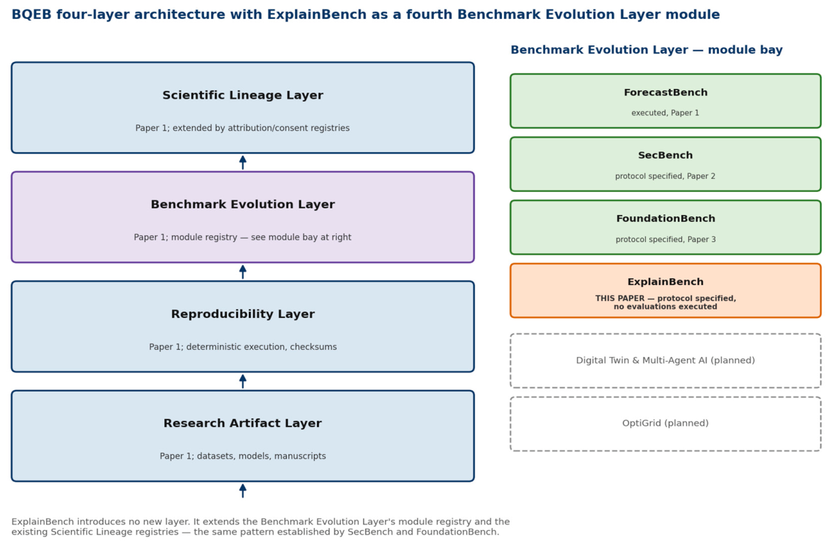
Figure 2.
ExplainBench metric hierarchy: component metrics feeding composite indices, evaluated against the registered XAI methods. No numeric value shown is a result; this figure is a structural map.
Figure 2.
ExplainBench metric hierarchy: component metrics feeding composite indices, evaluated against the registered XAI methods. No numeric value shown is a result; this figure is a structural map.
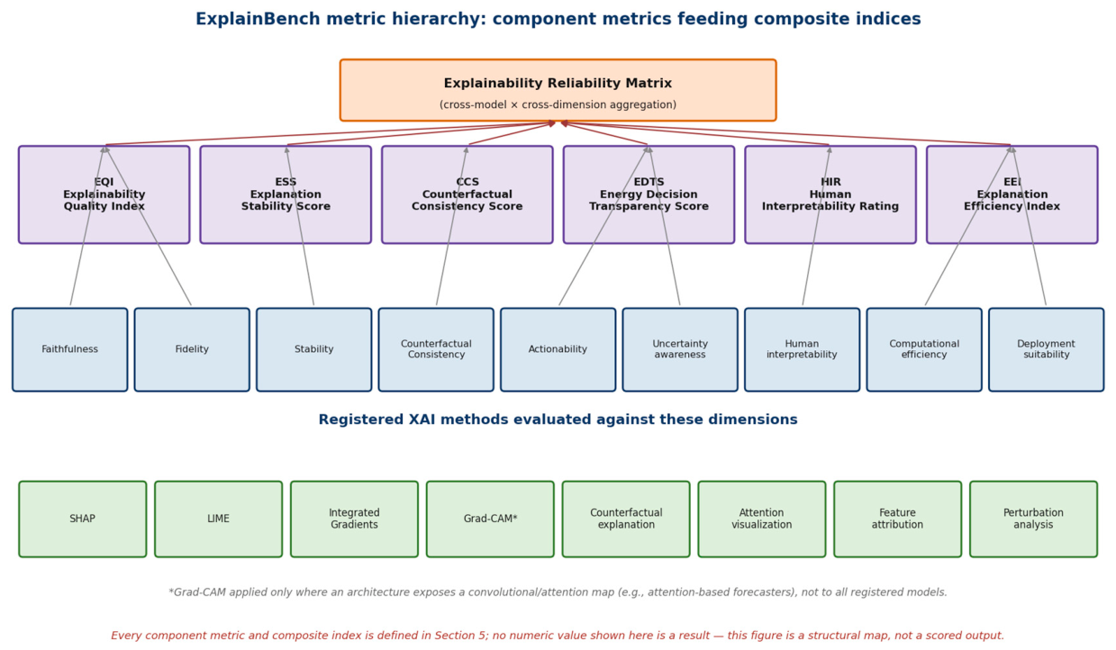
Table 4.
a. Composite index design rationale, supplementing Table 4's metric inventory.
Table 4.
a. Composite index design rationale, supplementing Table 4's metric inventory.
| Composite | Components | Rationale |
| EQI | Faithfulness + Fidelity | Measures whether explanations accurately represent model reasoning |
| ESS | Stability | Measures robustness under perturbation |
| CCS | Counterfactual Consistency | Measures reliability of alternative explanations |
| EDTS | Actionability + Uncertainty Awareness | Measures operational decision transparency |
| HIR | Human Interpretability | Measures human usability |
| EEI | Efficiency + Deployment Suitability | Measures edge-deployment feasibility |
Table 4.
b. Deployment Suitability Score (DSS) dimensions (Eq. 12, Section 5.4). All dimensions are protocol-disclosed measurements, not fitted values; none has been executed at the time of writing (Section 9).
Table 4.
b. Deployment Suitability Score (DSS) dimensions (Eq. 12, Section 5.4). All dimensions are protocol-disclosed measurements, not fitted values; none has been executed at the time of writing (Section 9).
| Dimension | Measurement | Normalization |
| Hardware compatibility | Edge-device architecture compatibility | Binary/ordinal (0 = incompatible, 1 = fully compatible) |
| Memory efficiency | Peak memory footprint (MB) | Normalized 0–1 against device-class budget |
| Latency suitability | Inference latency (ms) | Normalized 0–1 against t_ref (Table 8) |
| Energy consumption efficiency | Energy per inference (joules) | Normalized 0–1 against device-class budget |
| Privacy deployment suitability | On-device vs. cloud-dependent processing constraint | Normalized 0–1 ordinal score |
Table 14.
Human Interpretability Rating Likert scale (Section 6.3), feeding the component metric h(e) in Eq. 7. Anchors are calibrated against the fixed example set before rating begins, per the protocol above.
Table 14.
Human Interpretability Rating Likert scale (Section 6.3), feeding the component metric h(e) in Eq. 7. Anchors are calibrated against the fixed example set before rating begins, per the protocol above.
| Scale point | Anchor | Interpretation |
| 1 | Not interpretable | Rater cannot use the explanation to predict or justify the decision |
| 2 | Weakly interpretable | Explanation provides minimal, largely unusable guidance |
| 3 | Moderately interpretable | Explanation is usable with noticeable effort or ambiguity |
| 4 | Interpretable | Explanation is clear and sufficient with minor gaps |
| 5 | Highly interpretable | Explanation is clear, sufficient, and directly actionable |
Table 1.
Explainability category taxonomy (Section 4). *Grad-CAM applies only where the underlying architecture exposes a convolutional or attention map.
Table 1.
Explainability category taxonomy (Section 4). *Grad-CAM applies only where the underlying architecture exposes a convolutional or attention map.
| Category | Definition | Registered methods |
| Attribution-based | Assigns an importance score to each input feature/timestep | SHAP, Integrated Gradients, feature attribution |
| Surrogate-based | Fits an interpretable local model and explains via the surrogate | LIME |
| Example-based | Explains via a contrastive or counterfactual instance | Counterfactual explanation |
| Attention-based | Explains via the model's own internal attention weights | Attention visualization, Grad-CAM* |
| Perturbation-based | Explains via systematic input perturbation and output-change observation | Perturbation analysis |
Table 2.
Registered forecasting models. Deployment mode follows FoundationBench's registry classification (Paper 3).
Table 2.
Registered forecasting models. Deployment mode follows FoundationBench's registry classification (Paper 3).
| Model | Architecture family | Deployment mode | Reference |
| Chronos | T5-style encoder-decoder; scaling + quantization tokenization | Open-weight, zero-shot | [22] |
| TimesFM | Decoder-only, patched Transformer | Open-weight, zero-shot | [23] |
| Moirai | Masked-encoder Transformer, universal | Open-weight, zero-shot | [24] |
| PatchTST | Channel-independent, patched Transformer | Supervised, per-dataset | [25] |
| Informer | Decoder-only Transformer, ProbSparse attention | Supervised, per-dataset | [26] |
| Autoformer | Decomposition Transformer, auto-correlation | Supervised, per-dataset | [27] |
| LSTM | Recurrent (gated) | Supervised, per-dataset | [28] |
| Transformer | Standard encoder-decoder attention | Supervised, per-dataset | [29] |
Table 3.
Registered XAI methods. *Grad-CAM restricted to architecture-appropriate models per Table 9's compatibility matrix. Determinism determines whether stability estimation (Eq. 3) requires averaging over repeated runs.
Table 3.
Registered XAI methods. *Grad-CAM restricted to architecture-appropriate models per Table 9's compatibility matrix. Determinism determines whether stability estimation (Eq. 3) requires averaging over repeated runs.
| Method | Category | Deterministic given fixed seed? | Reference |
| SHAP | Attribution-based | No (sampling-based) | [30] |
| LIME | Surrogate-based | No (sampling-based) | [31] |
| Integrated Gradients | Attribution-based | Yes (fixed baseline) | [32] |
| Grad-CAM* | Attention-based | Yes | [33] |
| Counterfactual explanation | Example-based | No (search-based) | [19] |
| Attention visualization | Attention-based | Yes | — |
| Feature attribution (general) | Attribution-based | Method-dependent | — |
| Perturbation analysis | Perturbation-based | Yes (fixed perturbation set) | — |
Table 4.
Complete metric inventory cross-referenced to Section 5's equations.
Table 4.
Complete metric inventory cross-referenced to Section 5's equations.
| Metric | Type | Equation | Feeds |
| Faithfulness (F) | Component | Eq. 1 | EQI |
| Fidelity (Fid) | Component | Eq. 2 | EQI |
| Stability (S) | Component | Eq. 3 | ESS |
| Counterfactual Consistency | Component/Composite | Eq. 4 | CCS |
| Actionability (Act) | Component | Eq. 5 | EDTS |
| Uncertainty Awareness (UA) | Component | Eq. 6 | EDTS |
| Human Interpretability (h) | Component | Eq. 7 | HIR |
| Computational Efficiency (Eff) | Component | Eq. 8 | EEI |
| Deployment Suitability | Component | Eq. 12 (DSS, Section 5.4) | EEI |
| EQI | Composite | Eq. 9 | Reliability Matrix |
| ESS | Composite | Sec. 5.2 | Reliability Matrix |
| CCS | Composite | Eq. 4 | Reliability Matrix |
| EDTS | Composite | Eq. 10 | Reliability Matrix |
| HIR | Composite | Sec. 5.2 | Reliability Matrix |
| EEI | Composite | Eq. 11 | Reliability Matrix |
Table 5.
Comparison with prior explainability benchmarks across eight dimensions. ExplainBench's distinguishing contribution is energy-specific scope, time-series forecasting explanation, edge-deployment constraints, and versioned reproducibility infrastructure integrated with Papers 1–3 — not broader modality coverage, which all three prior efforts exceed.
Table 5.
Comparison with prior explainability benchmarks across eight dimensions. ExplainBench's distinguishing contribution is energy-specific scope, time-series forecasting explanation, edge-deployment constraints, and versioned reproducibility infrastructure integrated with Papers 1–3 — not broader modality coverage, which all three prior efforts exceed.
| Dimension | ERASER [5] | M4 [21] | Quantus [36] | ExplainBench (this work) |
| Domain | General NLP | General (image, text) | General (image, text, tabular, time-series) | Energy-exclusive |
| Model type | Text classifiers | 10+ deep models | Neural networks (framework-agnostic) | 8 energy-forecasting models |
| Explanation type | Extractive rationales | Feature attribution | 35+ metrics, 6 categories | 5 taxonomy categories (Table 1) |
| Time-series support | No | No | Declared, not domain-specialized | Yes (core focus) |
| Energy domain | No | No | No | Yes (6 deployment contexts) |
| Human evaluation | No | No | No (documented limitation) | Yes (HIR, Section 6.3) |
| Reproducibility infrastructure | Public benchmark; not versioned against a governed architecture | Public benchmark; not versioned against a governed architecture | Open-source toolkit; not a governed benchmark architecture | Integrates with Papers 1–3's versioned, checksummed registry infrastructure |
Table 6.
Energy-domain deployment contexts (Section 6.1 and Section 6.2). Not an exhaustive taxonomy of energy AI applications; scoped to contexts where an on-device agent's forecast or recommendation is the object being explained.
Table 6.
Energy-domain deployment contexts (Section 6.1 and Section 6.2). Not an exhaustive taxonomy of energy AI applications; scoped to contexts where an on-device agent's forecast or recommendation is the object being explained.
| Domain | Representative on-device agent | Primary decision explained |
| Smart-grid edge agents | Substation/feeder-level autonomous controller | Dispatch-relevant load/price forecast |
| Home energy management (HEMS) | On-device thermostat/battery/EV-charger scheduler | Load-shifting recommendation |
| Building energy management (BEMS) | Commercial building automation agent | HVAC/load optimization decision |
| Industrial energy IoT | Plant-level energy optimization agent | Consumption scheduling decision |
| EV charging / V2G | Charging station or vehicle-side controller | Charge/discharge timing decision |
| Renewable microgrid controllers | Solar/wind/battery microgrid balancing agent | Generation-demand balancing decision |
Table 7.
Benchmark tasks (Section 6.2). Tasks 1-2 reuse ForecastBench's existing forecasting targets; Task 3 varies deployment context rather than target.
Table 7.
Benchmark tasks (Section 6.2). Tasks 1-2 reuse ForecastBench's existing forecasting targets; Task 3 varies deployment context rather than target.
| Task | Target | Purpose |
| Task 1: Load-forecast explanation quality | Next-hour electricity load (reused from ForecastBench) | Evaluate explanation quality for the load-forecasting target |
| Task 2: Price-forecast explanation quality | Day-ahead electricity price (reused from ForecastBench) | Evaluate explanation quality for the price-forecasting target |
| Task 3: Cross-domain explanation quality | Same model/method, varied deployment context (Table 6) | Isolate domain-specific effects on Actionability and Deployment Suitability |
Table 8.
Evaluation protocol parameters (Section 6.4). Default equal weighting is a disclosed protocol choice, not a fitted value; sensitivity to alternative weightings is reserved for the ablation study (Section 9).
Table 8.
Evaluation protocol parameters (Section 6.4). Default equal weighting is a disclosed protocol choice, not a fitted value; sensitivity to alternative weightings is reserved for the ablation study (Section 9).
| Parameter | Symbol | Default value | Used in |
| Perturbation ball radius | eps | Protocol-versioned constant | Stability (Eq. 3) |
| Local neighborhood sample size | |N(x)| | Protocol-versioned constant | Fidelity (Eq. 2) |
| Bootstrap resample count | B | 10,000 | All composite CIs (Algorithm 4) |
| Counterfactual run count | M | Protocol-versioned constant | CCS, Actionability (Eqs. 4-5) |
| EQI weights | w1, w2 | 0.5, 0.5 (default equal) | Eq. 9 |
| EDTS weights | w3, w4 | 0.5, 0.5 (default equal) | Eq. 10 |
| EEI weights | w5, w6 | 0.5, 0.5 (default equal) | Eq. 11 |
| Human rater panel size | R | Protocol-versioned constant | HIR (Eq. 7) |
Table 9.
Model x method compatibility matrix (Section 3.2). Grad-CAM and attention visualization require an exposed attention/convolutional map; Autoformer's auto-correlation mechanism and the standard LSTM do not expose one in their reference implementations.
Table 9.
Model x method compatibility matrix (Section 3.2). Grad-CAM and attention visualization require an exposed attention/convolutional map; Autoformer's auto-correlation mechanism and the standard LSTM do not expose one in their reference implementations.
| Model | SHAP | LIME | Int. Grad. | Grad-CAM | Counterfactual | Attention | Feat. Attr. | Perturbation |
| Chronos | Yes | Yes | Yes | No | Yes | Yes | Yes | Yes |
| TimesFM | Yes | Yes | Yes | No | Yes | Yes | Yes | Yes |
| Moirai | Yes | Yes | Yes | Yes | Yes | Yes | Yes | Yes |
| PatchTST | Yes | Yes | Yes | Yes | Yes | Yes | Yes | Yes |
| Informer | Yes | Yes | Yes | Yes | Yes | Yes | Yes | Yes |
| Autoformer | Yes | Yes | Yes | No | Yes | No | Yes | Yes |
| LSTM | Yes | Yes | Yes | No | Yes | No | Yes | Yes |
| Transformer | Yes | Yes | Yes | Yes | Yes | Yes | Yes | Yes |
Table 10.
Failure mode taxonomy. Each mode is independently diagnosable from a single component metric, by design — an explanation can fail on one dimension while scoring well on the others, which a single composite score alone would not reveal.
Table 10.
Failure mode taxonomy. Each mode is independently diagnosable from a single component metric, by design — an explanation can fail on one dimension while scoring well on the others, which a single composite score alone would not reveal.
| Failure mode | Symptom | Diagnostic metric |
| Unfaithful | Explanation does not reflect what actually drives the model's output | Low Faithfulness (Eq. 1) |
| Unstable | Small input perturbations produce disproportionate explanation changes | Low Stability (Eq. 3) |
| Inconsistent counterfactuals | Repeated counterfactual searches disagree with each other | Low CCS (Eq. 4) |
| Non-actionable | Counterfactual implies a change an operator cannot execute | Low Actionability (Eq. 5) |
| Miscalibrated | Explained confidence does not match empirical accuracy | Low Uncertainty Awareness (Eq. 6) |
| Uninterpretable | Human raters cannot use the explanation to predict or justify the decision | Low Human Interpretability (Eq. 7) |
| Latency-infeasible | Explanation generation exceeds the edge-deployment latency budget | Low Computational Efficiency (Eq. 8) |
Table 11.
Benchmark Configuration Matrix. 64 = 8 models x 8 methods; 58 valid pairs after excluding architecture-incompatible combinations per Table 9 (6 excluded: Grad-CAM for Chronos and TimesFM; Grad-CAM and Attention visualization each for Autoformer and LSTM).
Table 11.
Benchmark Configuration Matrix. 64 = 8 models x 8 methods; 58 valid pairs after excluding architecture-incompatible combinations per Table 9 (6 excluded: Grad-CAM for Chronos and TimesFM; Grad-CAM and Attention visualization each for Autoformer and LSTM).
| Configuration axis | Count | Restricted by |
| Registered forecasting models | 8 | Table 2 |
| Registered XAI methods | 8 | Table 3 |
| Valid (model, method) pairs | 58 of 64 possible | Table 9 compatibility map |
| Energy domains (Task 3 only) | 6 | Table 6 |
| Total Task 1-2 evaluation cells | 58 | 58 pairs x 2 tasks |
| Total Task 3 evaluation cells | 348 | 58 pairs x 6 domains |
Table 12.
Planned evaluation template (Chronos row, representative excerpt). 'Reserved' denotes reserved for future experimental validation; no values are estimated or implied. Grad-CAM is absent from this row per Table 9 (not applicable to Chronos), consistent with omitting rather than imputing incompatible cells.
Table 12.
Planned evaluation template (Chronos row, representative excerpt). 'Reserved' denotes reserved for future experimental validation; no values are estimated or implied. Grad-CAM is absent from this row per Table 9 (not applicable to Chronos), consistent with omitting rather than imputing incompatible cells.
| Method | EQI | ESS | CCS | EDTS | HIR | EEI |
| SHAP | Reserved | Reserved | Reserved | Reserved | Reserved | Reserved |
| LIME | Reserved | Reserved | Reserved | Reserved | Reserved | Reserved |
| Integrated Gradients | Reserved | Reserved | Reserved | Reserved | Reserved | Reserved |
| Counterfactual explanation | Reserved | Reserved | Reserved | Reserved | Reserved | Reserved |
| Attention visualization | Reserved | Reserved | Reserved | Reserved | Reserved | Reserved |
| Feature attribution | Reserved | Reserved | Reserved | Reserved | Reserved | Reserved |
| Perturbation analysis | Reserved | Reserved | Reserved | Reserved | Reserved | Reserved |
Table 13.
Reproducibility checklist, following the format established in Papers 1–3.
| Item | Status |
| Dataset publicly available with a persistent identifier | Yes (inherited from Paper 1) |
| Model registry versioned as a distinct registry | Specified, not yet implemented |
| Explanation-method registry versioned as a distinct registry | Specified (Section 3.1), not yet implemented |
| Deterministic execution (fixed seeds) for deterministic methods | Specified for compatible methods (Table 3) |
| Stochastic-method run count and seed sequence recorded | Specified as mandatory (Section 12) |
| Human rater calibration-set responses archived | Specified as mandatory (Section 12) |
| Naive/reference baseline reported alongside all results | Not applicable (no accuracy baseline; see Section 9) |
| Statistical validation (bootstrap CIs, corrected significance tests) | Specified (Section 8.7), not yet executed |
| Results independently verifiable via checksummed artifacts | Specified for deterministic methods; disclosed as weaker for stochastic methods pending seed-sequence archival |
Table 12.
a. Pilot validation scope summary. No component in this table has been executed at the time of writing; every status is disclosed, not implied.
Table 12.
a. Pilot validation scope summary. No component in this table has been executed at the time of writing; every status is disclosed, not implied.
| Component | Configuration | Status |
| Dataset | BQEB-Data v1 | Reserved |
| Models | LSTM, Transformer | Reserved |
| Explanation Methods | SHAP, Integrated Gradients, LIME | Reserved |
| Metrics | EQI, ESS, CCS, HIR, EEI | Reserved |
| Experimental Results | None reported | Future execution |
Table 13.
a. Pilot reporting template (Section 12.1). Every cell is reserved for future experimental execution; no value is estimated, implied, or approximated. EDTS is intentionally absent from this pilot's scope (see rationale above), not omitted by oversight.
Table 13.
a. Pilot reporting template (Section 12.1). Every cell is reserved for future experimental execution; no value is estimated, implied, or approximated. EDTS is intentionally absent from this pilot's scope (see rationale above), not omitted by oversight.
| Model | Explanation Method | EQI | ESS | CCS | HIR | EEI |
| LSTM | SHAP | Reserved for future experimental execution | Reserved for future experimental execution | Reserved for future experimental execution | Reserved for future experimental execution | Reserved for future experimental execution |
| LSTM | Integrated Gradients | Reserved for future experimental execution | Reserved for future experimental execution | Reserved for future experimental execution | Reserved for future experimental execution | Reserved for future experimental execution |
| LSTM | LIME | Reserved for future experimental execution | Reserved for future experimental execution | Reserved for future experimental execution | Reserved for future experimental execution | Reserved for future experimental execution |
| Transformer | SHAP | Reserved for future experimental execution | Reserved for future experimental execution | Reserved for future experimental execution | Reserved for future experimental execution | Reserved for future experimental execution |
| Transformer | Integrated Gradients | Reserved for future experimental execution | Reserved for future experimental execution | Reserved for future experimental execution | Reserved for future experimental execution | Reserved for future experimental execution |
| Transformer | LIME | Reserved for future experimental execution | Reserved for future experimental execution | Reserved for future experimental execution | Reserved for future experimental execution | Reserved for future experimental execution |
Disclaimer/Publisher’s Note: The statements, opinions and data contained in all publications are solely those of the individual author(s) and contributor(s) and not of MDPI and/or the editor(s). MDPI and/or the editor(s) disclaim responsibility for any injury to people or property resulting from any ideas, methods, instructions or products referred to in the content. |
© 2026 by the authors. Licensee MDPI, Basel, Switzerland. This article is an open access article distributed under the terms and conditions of the Creative Commons Attribution (CC BY) license.
Copyright: This open access article is published under a Creative Commons CC BY 4.0 license, which permit the free download, distribution, and reuse, provided that the author and preprint are cited in any reuse.