

Submitted:
22 August 2026
Posted:
02 September 2026
You are already at the latest version
Abstract
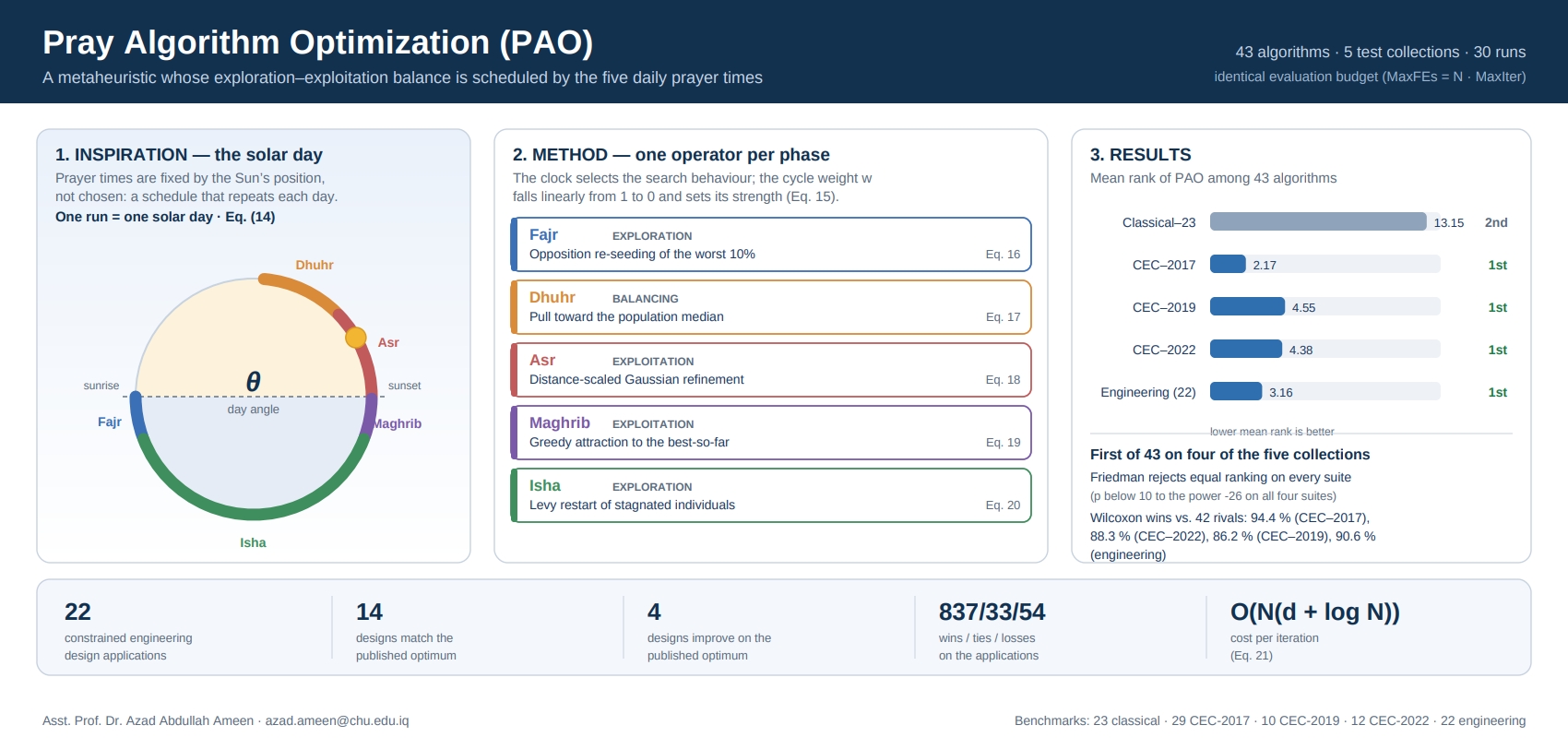
Most population-based metaheuristics govern the exploration–exploitation balance with a monotonically decreasing parameter, locking the search into fine-tuning early with no principled way to recover diversity. This paper introduces Pray Algorithm Optimization (PAO), whose schedule is derived from an external physical model rather than a decay rule chosen by hand: the run is mapped to a solar day, and the instantaneous solar altitude places five operators at the canonical Islamic prayer times, producing a non-monotone profile that restores diversity at fixed, planned points. PAO is validated against 42 competing algorithms over 75 benchmark functions — the classical 23-function set and the CEC-2017, CEC-2019 and CEC-2022 suites — with 30 runs of 500 iterations, and on 22 constrained engineering design problems. It ranks first of 43 algorithms on CEC-2017 (mean rank 2.17), CEC-2019 (4.55), CEC-2022 (4.38) and the engineering suite (2.96), and second on the classical set, where widespread ties at the global optimum compress the ranking. Friedman tests reject rank equality on every collection (p < 10⁻²⁶), and Wilcoxon win rates reach 86–94 % on the modern suites. On the engineering problems, PAO recovers or improves the reference optimum on 18 of 22 designs, attains the best solution found by any algorithm on 20, and is statistically net-positive against all 42 competitors. Diversity analysis shows an adaptive balance, from 4 % exploration on unimodal landscapes to 52 % on deceptive ones, while an ablation indicates the schedule acts chiefly as a variance-reduction mechanism. PAO ranks 36–41 of 43 in speed, though its complexity stays in the same class as standard swarm methods. Source code is available from the corresponding author.
Keywords:
metaheuristic optimization
; solar geometry
; prayer times
; global optimization
; exploration–exploitation balance
; CEC benchmark suites
; engineering design optimization
1. Introduction
This section explains why the paper exists. It describes what optimization problems are and why so many methods have been invented to solve them, then reviews the main families of these methods and how researchers group them. The review shows a gap: although algorithms have been drawn from animals, physics, chemistry, human society and mathematics, almost none has been built from the daily movement of the Sun. The section ends by stating what this paper contributes — a new optimizer called Pray Algorithm Optimization (PAO), built on the timing of the five daily prayers — and by listing the tests used to check whether it works.
1.1. Optimization and Its Reach
Optimization is, at its core, the search for the best available option among many. It appears wherever a resource is limited — time, money, raw material, energy, computing power — and wherever some quantity must be pushed as high or as low as the situation allows. Because limited resources are a permanent fact of life rather than a problem that appears now and then, optimization is less a specialized technique than a way of thinking that runs through nearly every applied field (Rajwar et al., 2023).Its reach is easy to underestimate. In engineering, optimization governs the sizing of structural members, the routing of transport and communication networks, and the calibration of manufacturing processes. In economics it underlies resource allocation, pricing policy, and the management of distribution systems. In artificial intelligence it drives model training, feature selection, and hyperparameter search; a clinical classifier for heart-disease prediction, for instance, gains measurable accuracy when its hyperparameters are tuned by a metaheuristic rather than fixed by hand(Hamajan, 2026). The same machinery reappears in sociology, in geology and resource exploration, and in genetics, where it supports sequence analysis and bioinformatic pipelines(Li et al., 2024). Everyday life differs only in stakes: deciding when to wake so that both sleep and deadlines are satisfied, or which route to take to work, are optimization decisions solved informally(Lang & Gao, 2025).What these cases share is a common structure, not a common subject. Once a problem has been written as a set of decision variables, a single measure of quality, and a set of constraints, the field it came from no longer matters. This is why optimization is sometimes called mathematical programming, and why a technique built for one field so often transfers unchanged to another. It is also why progress in optimization builds on itself: a single improvement in the underlying search machinery spreads at once to every field that uses the same formulation (Rajwar et al., 2023).
1.2. From Deterministic Methods to Metaheuristics
Optimization methods are usually divided into deterministic and heuristic families, with hybrid schemes drawing on both. A deterministic method follows a fixed sequence of steps and, given the same objective function and the same starting point, refollows the same path to the same answer every time. Heuristic methods add randomness on purpose: they give up the guarantee of identical results in exchange for the ability to climb out of the valley where the search happens to start (Darvishpoor et al., 2023).
For four decades the deterministic branch dominated engineering practice. Numerical linear and nonlinear programming — gradient descent, Newton and quasi-Newton schemes, sequential quadratic programming — are efficient, well understood, and on smooth convex models reliably reach the global optimum. The difficulty is that most real problems are none of those things. They need gradient information that may not exist; they contain many separate valleys, each with its own low point, so the answer returned depends on where the search began rather than on the problem itself; and where the objective or the constraints are rough and uneven, with sharp jumps, gradient-based procedures become unstable or fail clear (Tu et al., 2020). More detailed models have made this worse rather than better: as industrial and scientific models have grown in detail, obtaining a usable answer within an acceptable time has become harder, not easier (Li et al., 2024).
Metaheuristics were developed to work under exactly these conditions. They treat the objective as a black box (Boussaïd et al., 2013; Talbi, 2009a)— they only need to know the score a candidate solution receives, not how that score is computed. They require no derivatives, assume nothing about continuity or convexity, and combine fixed rules with random elements, often in a way borrowed from some natural or artificial process. Their appeal is as much practical as theoretical: they are simple to implement, easy to adapt to an unfamiliar problem, and ask almost nothing about how the model is built(Boussaïd et al., 2013).
Whatever metaphor a method adopts, its behavior is governed by two opposing forces. Exploration spreads the candidate solutions widely across the search space, searching for the region that holds the best overall answer; exploitation focuses effort around solutions already known to be good, refining them toward the best answer in their immediate neighborhood (Akbari et al., 2025). Randomness is what makes exploration possible, and it is also what allows a population to leave a local optimum once trapped in one. Too much exploration and search never stop moving long enough to converge; too much exploitation and it converges in the wrong place. Almost every design decision inside a metaheuristic is, in the end, a decision about how to move between these two modes, and when (Agrawal et al., 2021; Darvishpoor et al., 2023).
1.3. Research Activity in the Field
The result has been a rapid growth in numbers with few parallels in applied mathematics. More than five hundred distinct metaheuristics have now been published, a clear majority of them within the past decade, and the surrounding literature of surveys, comparative studies, and application papers has grown at a similar rate (Ameen, 2024; Rajwar et al., 2023; Shaikh et al., 2025). Research in the area falls into six recognizable streams (Ameen, 2024; Rajwar et al., 2023):
- Designing new algorithms, which accounts for the largest share of publications and for the taxonomy set out below. Five of the forty-two comparators illustrate the range. The Grey Wolf Optimizer guides a population using a ranking of leaders, with no velocity term (Mirjalili et al., 2014); Cuckoo Search uses Lévy-flight steps to widen the tail of the step-length distribution (Yang & Deb, 2009); the Honey Badger Algorithm alternates a digging phase with a honey-guided phase to switch between search modes (Hashim et al., 2022); the Archimedes Optimization Algorithm takes its operators from buoyancy and density rather than from animal behavior (Hashim et al., 2021); and the Circle Search Algorithm builds its update rule from the tangent relation on a circle, using no natural metaphor at all (Qais et al., 2022).
- Enhancement and modification of existing methods, where a known weakness is diagnosed and repaired. MRSO restructures the update rule of rat swarm optimization to correct an imbalance between its two search phases(Abdulla et al., 2024); EMRA revises the mud ring algorithm along comparable lines(Ali & Ameen, 2025); EMRSO adds hybrid memory strategies to MRSO (Hamid et al., 2026); EESB-FDO improves the fitness-dependent optimizer through a redesigned boundary-handling mechanism(Faraj et al., 2025); and DAOA replaces the static coefficients of the arithmetic optimization algorithm with dynamically varying ones(Khodadadi et al., 2022). The pattern is long established: L-SHADE adds linear population size reduction to SHADE and remains a standard baseline three decades after differential evolution itself(Tanabe & Fukunaga, 2014); a random-walk variant strengthens the exploration of the grey wolf optimizer (Gupta & Deep, 2019); an improved salp swarm algorithm sharpens its performance on feature selection (Hegazy et al., 2020); a chaotic dragonfly variant replaces random parameters with chaotic maps (Sayed et al., 2019); and an improved manta ray foraging optimizer was developed for multi-level image thresholding (Houssein et al., 2021).
- Hybridization, in which two methods are combined so that the strengths of one compensate for the weaknesses of the other. CDDO–HS, for example, couples child drawing development optimization with harmony search to improve information exchange within the population(Ameen, Rashid, & Askar, 2023). The pairing is usually chosen so that an exploratory method supplies breadth and an exploitative one supplies depth: PSO–GWO fuses the exploitation of particle swarm optimization with the exploration of the grey wolf optimizer (Şenel et al., 2019), and BGWOPSO carries the same pairing into binary feature-selection problems (Al-Tashi et al., 2019). Simulated annealing is a common partner for this reason, as in its hybrid with the whale optimization algorithm (Mafarja & Mirjalili, 2017). Earlier examples combine an ant colony with a genetic algorithm for protein function prediction (Nemati et al., 2009) and more recent ones pair a gradient-based optimizer with the grey wolf optimizer for human activity recognition (Helmi et al., 2021).
- Comparative analysis, which addresses the practical question of which algorithm to select for a given problem class. The scale of these studies has grown with the field; SFOA, for instance, was validated against one hundred competing optimizers(Zhong et al., 2025). The methodology of such comparisons has itself become a subject of study, with explicit guidelines now published on benchmark choice, baseline selection, parameter tuning, and statistical testing (LaTorre et al., 2021).
- Single- and multi-objective formulations, since real problems frequently involve several conflicting criteria and therefore have a set of best trade-off solutions rather than a single optimum. NSGA-II established the standard approach through elitist non-dominated sorting with a crowding-distance operator (Deb et al., 2002); MOEA/D instead decomposes the problem into scalar subproblems solved simultaneously (Q. Zhang & Li, 2007); MOPSO incorporates Pareto superiority into particle swarm optimization by way of an external repository (Coello et al., 2004); NSGA-III extends the framework to many objectives using a set of reference points (Deb & Jain, 2014); and the multi-objective grey wolf optimizer applies the same archive principle to a swarm method (Mirjalili et al., 2016)..
- Tutorials and surveys, which orient newcomers and periodically take stock of what has accumulated (Rajwar et al., 2023). Worked tutorials serve the same purpose at the level of a single algorithm, setting out its equations and iterations step by step so that a newcomer can reproduce it, as in the tutorial on child drawing development optimization (Ameen, Rashid, & Askar1, 2023).
1.4. Ways of Classifying Metaheuristic Algorithms
The field has grown in several different directions at once, and no single scheme sorts it completely. Which classification is useful depends on the question being asked. A reader who wants to know where an idea came from needs a different scheme from one who wants to know how much memory the method uses, how many parameters must be tuned before it will run, or whether it can be given to a parallel machine. Eighteen axes recur in the literature, and they fall into four natural groups: where the idea came from, how the search is organized, how the method is written and tuned, and what it searches. Table 1 and Figure 1 summarizes all eighteen; the paragraphs below set out each group in turn.
- Where the idea came from. The oldest question is whether the designer borrowed the idea from the natural world. Methods that did divide into swarm intelligence, built on the collective behavior of many simple agents, and evolutionary computation, built on selection and inheritance. Methods that did not are grouped as non-nature-inspired, tabu search being the clearest case, since its forbidden-move list comes from an idea about memory rather than from any living thing (Blum & Roli, 2003). Within the nature-inspired group, a second axis asks which part of nature: authors divide this into three subgroups (Siddique & Adeli, 2015), four (Fister et al., 2013; Rajwar et al., 2023), five (Safiri & Nikoofard, 2023; Shaikh et al., 2025), or six (Khoshniat et al., 2024). A third axis, more recent and more critical, asks how faithfully a method follows the process it claims to copy. A strongly inspired algorithm genuinely reproduces the mechanism; a weakly inspired one uses the metaphor as decoration, and its equations could have been written without ever naming the animal in the title (Sörensen et al., 2025; Steer et al., 2009).
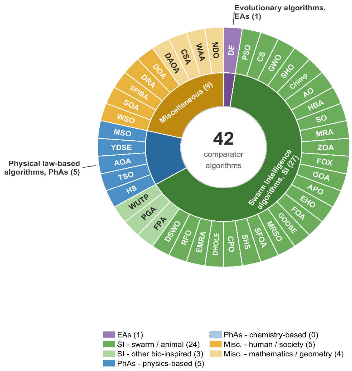
- How the search is organized. A second group of axes describes the machinery of the search itself. The most consequential counts how many candidate solutions are carried: one, as in tabu search, hill climbing and simulated annealing, or many, as in the genetic algorithm and ant colony methods (Jaddi & Abdullah, 2020). A second asks what the algorithm remembers. A memoryless method decides its next move from the current state alone and can look again at ground it has already covered; a method with memory keeps a record of earlier iterations and uses it to guide, which serves exploration and exploitation at the same time and usually pays for itself in fewer function evaluations. A third asks how a solution is assembled: an iterative method refines a candidate again and again, while a greedy method takes whatever looks best at each step and never revises it — faster and simpler, but it can easily miss the better answer that only becomes visible later (Sörensen et al., 2025). Two further axes, less often used but useful, ask whether the algorithm keeps one definition of which solutions count as neighbors or switches between several, as variable neighborhood search does, and whether it leaves the objective function alone or alters it during the run to push the search out of ground already visited, as guided local search does (Blum & Roli, 2003). A sixth asks how the next generation is actually produced: by shifting an existing solution, or by assembling a new one from several others, either through direct combination or through indirect coordination such as ant pheromone (Molina et al., 2020).Figure 1. Taxonomy of the 42 comparator algorithms by source of inspiration, after Rajwar et al. (2023): four families in the inner ring and one algorithm per segment in the outer ring, ordered by year within each family.Figure 1. Taxonomy of the 42 comparator algorithms by source of inspiration, after Rajwar et al. (2023): four families in the inner ring and one algorithm per segment in the outer ring, ordered by year within each family.
- How the method is written and tuned. A third group concerns the form of the algorithm rather than its behavior. Yang separates methods defined by a sequence of operations, such as evolution strategies and ant colony optimization, from those defined by explicit update equations, such as particle swarm optimization and cuckoo search; the great majority of modern methods are of the second kind, so what really separates one from another is the mathematical form of the update rule and not the set of terms of the metaphor (Yang, 2020). A newer axis simply counts the parameters a user must set before the method will run, grouping algorithms as free-parameter, mono-, bi-, tri-, tetra- and penta-parameter, with anything above five placed in a miscellaneous group; the fewer parameters a method carries, the less tuning it demands, which is why low-parameter methods are preferred for practical, real-world use (Rajwar et al., 2023). A related axis asks not how many parameters there are but how their values are set: on a fixed schedule, by feedback from the search, or by encoding them in the individuals so that they evolve with the population (Eiben et al., 1999).
- What is searched, and how it is deployed. A final group concerns the setting in which the method is used. A metaheuristic searches the space of solutions directly; a hyper-heuristic searches the space of heuristics, selecting or generating the low-level method that will then be applied, with generality rather than peak performance as the goal (Burke et al., 2013) .Methods also differ in whether they are defined as a single sequential process or as several processes running at once, since migration between subpopulations in an island model changes the search behavior and is not just a matter of how the code is written (Alba, 2005). They differ in the domain they natively address, continuous or binary, and a large share of published variants exist only to carry a continuous method into a binary setting by way of a transfer function (Pan et al., 2023). They differ in how they keep solutions within the rules. Some add a cost for breaking a rule; some use operators that cannot produce an illegal solution in the first place; some repair an illegal solution afterwards; and some treat rule-breaking as a separate measure to be reduced alongside the objective (Coello Coello, 2002). And they differ in how many criteria they optimize, a single-objective method returning one answer and a multi-objective method returns a set of trade-off solutions, called a Pareto front, in which no solution can be improved on one criterion without being made worse on another (Deb et al., 2002). Where two methods are combined, the combination itself can be classified by level, by order of execution, and by control strategy (Raidl, 2006; Talbi, 2009b).Table 1. Eighteen axes along which metaheuristic algorithms are classified. Every algorithm sits at a position on all eighteen simultaneously; the axes are complementary rather than competing.Table 1. Eighteen axes along which metaheuristic algorithms are classified. Every algorithm sits at a position on all eighteen simultaneously; the axes are complementary rather than competing.
# Axis One pole The other pole Reference 1 Source of the idea nature-inspired non-nature-inspired (Blum & Roli, 2003) 2 Domain of inspiration three to six subgroups — (Rajwar et al., 2023) 3 Strength of inspiration strong weak (Steer et al., 2009) 4 Candidates carried single solution population (Jaddi & Abdullah, 2020) 5 Use of memory memory-based memoryless (Yasear & Ku-Mahamud, 2019) 6 Assembly of a solution iterative greedy (Sörensen et al., 2025) 7 Neighborhood structures one several (Blum & Roli, 2003) 8 Objective function static dynamic (Blum & Roli, 2003) 9 Population movement vector movement solution creation (Molina et al., 2020) 10 Form of definition procedure-based equation-based (Yang, 2020) 11 Number of parameters free parameter up to penta- and beyond (Rajwar et al., 2023) 12 Parameter control fixed schedule adaptive or self-adaptive (Eiben et al., 1999) 13 What is searched solutions heuristics (hyper-heuristic) (Burke et al., 2013) 14 Execution sequential parallel or distributed (Alba, 2005) 15 Variable domain continuous binary or discrete (Pan et al., 2023) 16 Constraint handling penalty repair, feasible-only, separation (Coello Coello, 2002) 17 Number of objectives single objective multi-objective (Deb et al., 2002) 18 Hybrid structure high-level, collaborative low-level, integrative (Raidl, 2006)

These eighteen axes do not compete with one another. An algorithm has a position on every one of them at once: differential evolution is nature-inspired, evolutionary, population-based, memoryless, iterative, equation-based, bi-parameter, sequential by default and continuous by design. Three of the axes matter directly for what follows. The single- versus population-based distinction determines the class of method to which the present proposal belongs; the source of inspiration organizes the forty-two algorithms against which it is benchmarked; and the number of control parameters is the measure against which its own cost in tuning effort must later be assessed.
The single- versus population-based distinction is the most consequential for what follows. Single-solution methods such as simulated annealing and tabu search refine one candidate within its immediate neighborhood; they are economical and strongly exploitative, but a single trajectory can be captured by a local optimum with no mechanism for escape. Population-based methods instead maintain many candidates distributed across the search space, preserving diversity globally and sampling the landscape from several directions at once (Yang, 2020). This makes them markedly more robust on multimodal problems, and it is why essentially all recent proposals — including every algorithm considered in this study — are population-based (Jaddi & Abdullah, 2020).
1.5. Metaheuristics by Source of Inspiration
Within the population-based class, the most common organizing principle is the source of inspiration. It is also the oldest, and different authors partition it differently: into three subgroups (Siddique & Adeli, 2015), four (Fister et al., 2013), five (Safiri & Nikoofard, 2023; Shaikh et al., 2025), or six (Khoshniat et al., 2024; S. S. & H. S., 2022).
The present study adopts the four-subgroup scheme of Rajwar et al. (2023), which those authors identify as the most widely recognized of them, and which has the further value of dividing the physical-law family explicitly into a physics-based and a chemistry-based branch. The forty-two algorithms against which the present work is benchmarked are distributed across all four subgroups and are used below to illustrate each in turn; their distribution is shown in Figure 1, and their full details are given in Table 2.
- Evolutionary algorithms (EAs) are inspired by the Darwinian ideas of natural selection and the survival of those best suited to their surroundings. A population of individuals goes through simulated reproduction and mutation to create successive generations of offspring, the process being repeated so as to retain the genetic material that makes an individual better adapted to its environment while eliminating that which makes it weaker (Sloss & Gustafson, 2020). Darwin’s theory of natural evolution motivates both the genetic algorithm and differential evolution(Chakraborty et al., 2023), while genetic programming rests on the wider idea of biological evolution; gene expression programming, learning classifier systems, neuroevolutionary, and evolution strategies extend the same principle to other representations. Only one member of this family appears among the comparators. Differential Evolution remains the original model for the whole family and, three decades after its introduction, is still a serious competitor rather than a historical reference: its difference-vector mutation operator still sits at the heart of the best-performing entries in today’s optimization competitions (Tanabe & Fukunaga, 2014).
- Swarm intelligence (SI) algorithms model the collective behavior of systems that organize themselves with no central controller. Although Beni and Wang first used the term in 1989 in the context of cellular robotic systems, the term now covers any such system, and what marks these systems out is that they adapt as they go, communicate constantly, and share what they learn among agents that could neither defend themselves against a large hunting animal nor secure food alone (Rajwar et al., 2023). This is by a wide margin the largest family in literature, and it supplies twenty-seven of the forty-two comparators. Particle Swarm Optimization established the template, updating each particle from its own best position and the swarm’s (Abualigah et al., 2024; Kennedy & Eberhart, 1995); Cuckoo Search introduced Lévy-flight steps to widen the tail of the step-length distribution (Yang & Deb, 2009); and the Grey Wolf Optimizer later showed how a hierarchy of leaders could steer a population without an explicit velocity term (Mirjalili et al., 2014). Twenty-one further animal-behavior optimizers propose different mechanisms for regulating the same underlying trade-off: the Spotted Hyena Optimizer (Dhiman & Kumar, 2017), the Chimp Optimization Algorithm (Khishe & Mosavi, 2020), the Aquila Optimizer (Abualigah et al., 2021), the Honey Badger Algorithm (Hashim et al., 2022), the Snake Optimizer (Hashim & Hussien, 2022), the Mud Ring Algorithm (Desuky et al., 2022), the Zebra Optimization Algorithm (Trojovská et al., 2022), FOX (H. Mohammed & Rashid, 2023), the Gazelle Optimization Algorithm (Agushaka et al., 2023), Arctic Puffin Optimization (Wang et al., 2024), the Elk Herd Optimizer (Al-Betar et al., 2024), the Fossa Optimization Algorithm (Hamadneh et al., 2024), GOOSE (Hamad & Rashid, 2024), Modified Rat Swarm Optimization (Abdulla et al., 2024), the Starfish Optimization Algorithm (Zhong et al., 2025), the Scorpion Hunting Strategy (Singh et al., 2024), the Chinese Pangolin Optimizer (Guo et al., 2025), the Dhole Optimization Algorithm (B. O. Mohammed et al., 2025), the enhanced Mud Ring Algorithm (Ali & Ameen, 2025), Rüppell’s Fox Optimizer (Braik & Al-Hiary, 2025b), and Dwarf Sperm Whale Optimization (J. Zhang, 2026). A smaller non-swarm branch of the same bio-inspired family models plant rather than animal behavior: the Flower Pollination Algorithm (Yang, 2012), the Phototropic Growth Algorithm (Bohat et al., 2025), and an optimizer derived from water uptake and transport in plants (Braik & Al-Hiary, 2025a).
- Physical law-based algorithms (PhAs) encode physical or chemical law directly in the update rule, which often gives cleaner mathematics than a behavioral analogy. Rajwar (Rajwar et al., 2023) divide the family in two. Physics-based methods take gravitation, fields, the big bang, the black hole, and the galaxy as their primary sources, as in simulated annealing, the gravitational search algorithm, central force optimization, charged system optimization, electro-magnetism optimization, the big bang–big crunch algorithm, the black hole algorithm, and the galaxy-based search algorithm. Chemistry-based methods instead model molecular reaction, Brownian motion, and molecular radiation, as in gases Brownian motion optimization, the artificial chemical process, the ions motion optimization algorithm, and thermal exchange optimization. Four comparators fall in the physics-based branch: Transient Search Optimization, which borrows the response of a switched electrical circuit (Qais et al., 2020); the Archimedes Optimization Algorithm, whose operators derive from buoyancy and density (Hashim et al., 2021); the Young’s Double-Slit Experiment optimizer, which maps interference fringes onto search intensity (Abdel-Basset et al., 2023); and Mirage Search Optimization, which models atmospheric refraction (He et al., 2025). None of the forty-two takes up the chemistry-based branch. This family is of particular relevance here, since the present work draws on a physical system of the same kind.
- Miscellaneous is the residual subgroup, and in the formulation adopted here it collects methods founded on human behavior, game strategy, mathematical theorems, politics, artificial thought, and comparable ideas belonging to none of the preceding three (Rajwar et al., 2023). Ten comparators fall here, in two clearly separate groups. The first abstracts social, cognitive, or institutional processes. Harmony Search, modelled on a musician’s search for pleasing chords, is the long-standing representative (Zong Woo Geem et al., 2001); more recent entries include War Strategy Optimization (Ayyarao et al., 2022), the Skill Optimization Algorithm (Givi & Hubalovska, 2023), the Social Psychology Interaction Behavior Algorithm (Ameen, 2024), the Divine Religions Algorithm (Mozhdehi et al., 2025), and the Dream Optimization Algorithm (Lang & Gao, 2025). The Divine Religions Algorithm (Mozhdehi et al., 2025) is notable in the present context: it demonstrates that inspiration drawn from religious and social organization can yield a competitive optimizer and can be published in a well-regarded journal, provided the mathematics is stated independently of the metaphor. The second branch does away with natural inspiration altogether and constructs its operators from analytical or geometric objects. The Dynamic Arithmetic Optimization Algorithm builds its search on the four elementary arithmetic operators (Khodadadi et al., 2022); the Circle Search Algorithm exploits the tangent relation on a circle (Qais et al., 2022); the Weighted Average Algorithm updates from a weighted mean of the population (Cheng & De Waele, 2024); and the Newton Downhill Optimizer adapts a classical root-finding scheme to stochastic search (Xiao et al., 2026). Their advantage is transparency: the mechanism can be inspected directly, without decoding a metaphor first.
1.6. Limitations and Open Problems
Population-based methods are not without cost. They use far more memory and computation than single-solution alternatives, particularly at large population sizes or on expensive objective functions (Payerle et al., 2023). They fit naturally with parallel and distributed execution, which recovers part of that cost (Pardo et al., 2024), but they remain vulnerable to premature convergence: once population diversity collapses, the search stops making progress in whatever region it happens to be in, and most designs provide no mechanism for recovering the diversity that has been lost (Agrawal et al., 2021; Omeka et al., 2024).
These considerations set the requirements for any new proposal. It must balance exploration against exploitation rather than favoring either; it must maintain population diversity for long enough to avoid stagnation; and it must have reliably across problem classes rather than excelling on one family and failing badly on another. As well as these performance requirements, the field has begun to apply a further requirement about method. A substantial body of critical work argues that many recent metaheuristics contribute a new metaphor without contributing a new search mechanism — that once the terminology is removed, the update equations reduce to reparameterizations of methods already in the literature (Aranha et al., 2022; Dorigo, 2020; Sörensen & Glover, 2013).
The No Free Lunch theorem (Wolpert & Macready, 1997)supplies the formal justification for continuing to develop new methods at all. It establishes that, averaged over the space of all possible objective functions, no search algorithm outperforms any other: superior performance on one class of landscapes must be paid for by inferior performance on another (Velasco et al., 2024). The theorem therefore allows the search for algorithms whose inductive biases suit, practically important problem classes, while ruling out any claim of universal dominance. It is an argument for principled specialization, not for unlimited rapid growth in number (Velasco et al., 2024).
1.7. Motivation: Solar Geometry as a Control Schedule
Against that background, this work addresses a specific and, to our knowledge, unexamined weakness. Nearly every population-based metaheuristic requires some schedule for shifting emphasis from exploration to exploitation as the run proceeds, and in practice that schedule is almost always a hand-set value that only ever gets smaller — the linear decay of GWO, the quadratic and exponential decays used elsewhere, or a chaotic map substituted when additional variability is wanted. Such schedules share three defects. Being monotonic, they cannot re-expand the search radius once diversity has been lost. Their functional form and constants are chosen by the designer rather than derived, which adds tuning burden and obscures why one choice should be preferred to another. And they carry no physical meaning, so there is no principled basis for preferring any particular form.
Solar geometry offers an alternative that is free of all three defects, and it occupies a position that the taxonomy above leaves noticeably empty. Astronomical inspiration belongs formally to the physics-based branch of PhAs, whose recognized sources are gravitation, fields, the big bang, the black hole, and the galaxy; yet within that branch no established method draws on the observational geometry of the Earth–Sun system. Although optimizers have been derived from optics, electrical transients, buoyancy, and atmospheric refraction, and although cosmological objects have supplied metaphors for a generation of physics-based methods, the apparent motion of the Sun across the sky, and the shadow geometry that follows from it, have attracted almost no attention. For an observer at latitude on day of the year, the solar altitude angle — obtained from the solar declination and hour angle by the standard spherical-astronomy relation — traces a smooth and strictly non-monotonic curve that rises from below the horizon, peaks at solar transit, and descends again. The associated shadow ratio, cot , behaves exactly as one would want a step-size coefficient to behave it diverges near sunrise and sunset, when the Sun is low and shadows are long, and contracts to a minimum at solar noon. A search radius driven by shadow length is therefore wide during the opening and closing situations of the cycle and narrow at its center, and it recovers automatically rather than decaying irreversibly. The whole schedule follows from and through closed-form trigonometric expressions containing no fitted constants, so an entire family of schedules is available at zero tuning cost.
The five canonical Islamic prayer times supply the natural partition of this curve. Fajr, Dhuhr, Asr, Maghrib, and Isha are not chosen by hand divisions of the day; each is fixed by an explicit geometric condition on the Sun’s position — Fajr and Isha by angle of the Sun below the horizon at twilight angles below the horizon, Dhuhr by the instant of solar transit, Asr by a prescribed ratio between an object’s shadow and its own length, and Maghrib by the disappearance of the solar disc corrected for atmospheric refraction. These conditions have been evaluated by standard astronomy for more than a thousand years, and they constitute a well-established segmentation of the solar cycle into five intervals of distinct geometric character: two low-altitude twilight regimes, one transit regime, one shadow-ratio regime, and one horizon-crossing boundary event. It is this partition, rather than the metaphor as such, that the proposed algorithm exploits.
1.8. Contributions and Organization of the Paper
The present study therefore introduces the Pray Algorithm Optimizer (PAO), a population-based metaheuristic whose control schedule and search radius are derived from solar altitude and shadow ratio, and whose search proceeds through five operators corresponding to the five prayer intervals. Across one solar day the controller switches on at most one extra operator per iteration, and the five together span the full range of search behaviors. Fajr restarts the worst individuals by reflecting them through the center of the search box to the point directly opposite, injecting long-range diversity that a contracted population can no longer produce on its own. Dhuhr draws a random subset part of the way toward the population median — a neighborhood statistic that settles the swarm without locking it to any single region. Asr and Maghrib both rely on global information, the best solution found so far, but to opposite ends: Asr takes small, distance-scaled Gaussian steps that refine individuals already close to the best, whereas Maghrib pulls its subset part of the way straight toward it, most strongly late in the run. Isha closes the cycle by giving stagnated individuals a heavy-tailed Lévy jump, restoring the diversity that the exploitative phases have used up. Underneath all five, the base engine of Section 3.4 supplies the two-at-a-time, difference-based mutation that runs on every iteration, so the phase operators add to rather than replace it.
The main contributions of this study are as follows:
- A new population-based metaheuristic, PAO, whose exploration–exploitation schedule and search radius are obtained in closed form from spherical-astronomy relations for solar altitude and shadow ratio, rather than from a hand-designed decay function. This places it in an inspiration category — astronomical — that is essentially unoccupied in the current literature.
- A non-monotonic, parameter-free control schedule that allows search diversity to be recovered in the later stages of a run, in contrast to the monotonically decreasing coefficients used by the majority of existing methods.
- Five structurally distinct search operators derived from the geometric conditions that define the five prayer intervals, together with an explicit term-by-term demonstration that the resulting update rules are not reparameterizations of PSO, DE, GWO, or SCA.
- A large-scale empirical evaluation against forty-two algorithms published between 1995 and 2026 and spanning all four inspiration families, on seventy-five benchmark functions: 23 classical functions, 30 CEC2017 functions, 10 CEC2019 functions, and 12 CEC2022 functions, under a uniform protocol of identical population size, identical evaluation budget, and 30 independent runs.
- A complete statistical treatment comprising 3,150 pairwise Wilcoxon rank-sum comparisons, Friedman rank analysis with post-hoc procedures, convergence and boxplot analysis, and a runtime comparison.
- A population-size sensitivity study over N ∈ {20, 30, 40, 50, 60} across all four benchmark suites.
- Application to 22 real-world engineering and application problems: Speed reducer (gearbox), Tension/compression spring, Pressure vessel, Three-bar truss, Gear train ratio, Cantilever beam, I-beam deflection, Tubular column, Piston lever, Car side impact, Welded beam, Reinforced concrete beam, Multi-disk clutch brake, Rolling element bearing, Belleville disc spring, Hydrostatic thrust bearing, Robot gripper, Gas transmission compressor, Stepped cone pulley, Planetary gear train, 10-bar planar truss (FEM), Heat exchanger (Himmelblau)
- Public release of the PAO source code at [ https://www.mathworks.com/matlabcentral/fileexchange/184442-pao-for-global-and-constrained-engineering-optimization ], so that the results reported here can be reproduced independently.
The remainder of this paper is organized as follows. Section 2 develops the astronomical background, including the computation of solar position and of the five prayer times. Section 3 presents PAO, its mathematical model, pseudocode, complexity analysis, and its relationship to existing algorithms. Section 4 describes the experimental protocol. Section 5 reports and discusses the benchmark results. Section 6 applies PAO to real-world engineering problems. Section 7 discusses limitations, and Section 8 concludes.
2. Astronomical Background and Inspiration
This section explains the idea behind the algorithm before any mathematics is applied to it. It first describes the five daily prayers and the fact that their times are not chosen by people but fixed by the position of the Sun. It then shows how the Sun’s position can be written as a single angle that moves through one full turn each day, and how each prayer time corresponds to a particular value of that angle. The key point for the reader is that this gives a natural, repeating schedule that changes with the season and with where you are on Earth — exactly the kind of schedule an optimizer needs when it has to switch between wide searching and careful refining.
2.1. Prayer in Islam and the Determination of Prayer Times
Prayer (ṣalāh) is one of the five main practices of Islam, and the five daily prayers are something every adult Muslim is required to perform. Like the other main religious duties — paying zakat and giving voluntary charity (ṣadaqah), and dividing the property a person leaves behind after death — prayer is not left to each person to decide. Its number, the way it is performed, and above all its times are set by Islamic law (the Sharia) through its two main sources, the Qur’an and the Sunnah (Bahri & Hasibuan, 2024; Esposito, 2011).
That the five daily prayers must be performed at fixed times is a rule from the holy texts, not just a custom: the Qur’an describes prayer as a duty that must be done at set times, and the Prophetic tradition (Sunnah) gives, for each of the five, a starting point marked by a visible position of the Sun. So the rules for when each prayer may be performed belong to Islamic religious law (fiqh) just as much as to astronomy, and the two meet exactly at the point where a religiously defined moment has to be turned into a clock time (Rojak & Fawzi, 2024).
Each prayer begins when the Sun reaches a stated position — sitting a fixed distance below the horizon before sunrise, crossing the highest point of the sky, shadows growing to a set length, the Sun sinking below the horizon, and the evening light fading after sunset. Because these are astronomical events, the prayer times change from place to place and from day to day. Three things move them: where the observer is on Earth, given by latitude and longitude; the date, and so the time of year (season), through the Sun’s changing declination; and the rules chosen by the different schools of Islamic law (Bahri & Hasibuan, 2024; Meeus, 1991; Rojak & Fawzi, 2024).
The four Sunni schools of law — Hanafi, Shafi’i, Maliki, and Hanbali — agree on the astronomical events that mark the five prayers but differ on some of the exact points used to read them. The clearest difference is the afternoon prayer, ʿAṣr: the Shafi’i, Maliki, and Hanbali schools start it when an upright object’s shadow has grown by an amount equal to the object’s own height beyond its noon length, while the Hanafi school waits until the added shadow equals twice that height. There are also smaller differences in how far below the horizon the Sun must be at dawn and dusk (the twilight angles) for Fajr and Isha. These differences are why published prayer timetables for the same city on the same day do not always match, and why any calculation must state which rule it follows (Rojak & Fawzi, 2024).
What matters for this work is that the five prayer moments split the whole day using geometry alone: once we know a latitude, a date, and a chosen school’s rule, their positions come straight from the position of the Sun, with no free number left to adjust by hand. This is exactly the property PAO reuses — a smooth, repeating, up-and-down schedule set entirely by astronomy — turning it into a control schedule for optimization, as the rest of this section explains.
2.2. The Idea in Plain Terms
Every population-based optimizer needs a rule that decides, at each moment of a run, how far its candidate solutions should move. Early on, long moves are wanted, because the search must cover ground; later, short moves are wanted, because the best solution found so far needs fine-tuning rather than replacing. In almost all existing algorithms this rule is a hand-made number that only ever decreases.
PAO takes the rule from somewhere else: the position of the Sun during a single day. The Sun rises, climbs to its highest point, and sets. The shadow it casts is long at the two ends of the day and short in the middle. That pattern has four properties that are useful here. It is smooth. It is not monotone, so the quantity driven by it can grow again after getting smaller. It repeats exactly. And it is fixed completely by two numbers — the latitude of the observer and the day of the year — with no constant left for the designer to choose.
The five daily Islamic prayers divide this curve at instants that are themselves defined geometrically rather than by convention: two are fixed by how far the Sun sits below the horizon, one by the instant the Sun crosses the meridian, one by the ratio of an object’s shadow to its own length, and one by the Sun touching the horizon. The result is a partition of the day into intervals of distinct geometric character. PAO gives each interval its own search operator.
2.3. Where the Sun is
Let be the day of the year and let be the latitude of the observer, positive north. The declination is the angle between the Sun’s rays and the plane of the Earth’s equator; it varies slowly through the year and is given to sufficient accuracy by Cooper’s equation (Cooper, 1969; Duffie & Beckman, 2013):
Local time is measured by the hour angle , which is zero at solar noon and advances by 15° for every hour. Writing for clock time in minutes after midnight (Duffie & Beckman, 2013; Ma & Iqbal, 1983),
The height of the Sun above the horizon, the solar altitude , then follows from a standard astronomy formula(Duffie & Beckman, 2013; Meeus, 1991):
Two quantities derived from are used later. The zenith angle measures the Sun’s distance from straight overhead, and the shadow ratio is the length of the shadow cast by a vertical object of unit height (Ma & Iqbal, 1983):
The shadow ratio is the quantity that behaves like a search radius. It becomes very large when the Sun is low, near sunrise and sunset, and reaches its minimum at solar noon. A step-size driven by it is therefore wide at the two ends of the cycle and narrow in the middle, and it widens again on its own rather than decaying once and for all.
2.4. Reading the Geometry Backwards
Prayer times are defined by the Sun reaching a stated height, so has to be solved for rather than evaluated. Rearranging gives the hour angle at which the altitude equals a set prescribed value α (Meeus, 1991):
Sunrise and sunset are the case , the small negative value accounting for atmospheric refraction and the radius of the solar disc. With the two instants and the length of the day are (Meeus, 1991):
2.5. The Five Prayer Times as Geometric Conditions
Each prayer begins when the Sun satisfies one specific geometric condition. Table 3 states them. Only Asr needs an extra formula: its condition is that the shadow of a vertical object has grown by times the object’s own height beyond its length at noon, with in the Shafi‘i, Maliki and Hanbali schools and in the Hanafi school. Converting that statement into an altitude gives(Bahri & Hasibuan, 2024; Rojak & Fawzi, 2024):
so follows immediately, and the corresponding instant follows from . In general, every prayer instant is obtained by substituting its altitude condition into :
with the minus sign before solar noon and the plus sign after it. Here _condition is not a fixed number but a placeholder for the solar altitude that defines the prayer in question: the value in the “Altitude used” column of Table 3 — for Fajr, for Isha, and for Maghrib — and, for Asr, the altitude from . Dhuhr is the exception: it is fixed by the Sun crossing the meridian (), not by a depression angle, so it is read directly rather than through .
2.6. A Clock that Lengthens with the Season
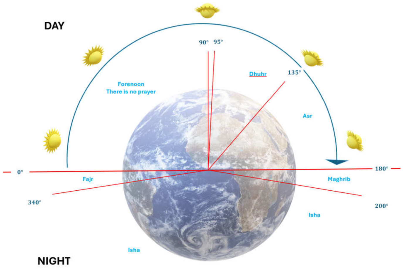
The five instants of Table 3 move as and change: near the equator they shift little, at high latitude they shift a great deal. If the algorithm referred to them by clock time, its schedule would have to be re-derived for every location and date. To avoid this, time is re-expressed as an angle that always completes one full turn over one day (see Figure 2), with sunrise at and sunset at . This remapping is introduced in the present work (Eqs. 8–9 are not a standard astronomical relation). Call it the day angle :
The inverse map, which converts an angle back to a clock time, is used to lay the five windows onto the run. Within daylight, is an affine function of the hour angle of , so it carries the same information; the piecewise definition simply forces night to occupy the same as day, whatever the season. The effect is that a window written in automatically stretches in summer and contracts in winter, and adapts to latitude, without a single number being changed.
Figure 3.
The day-angle representation θ that PAO uses to place the five prayer windows. Daylight is mapped onto θ ∈ [0°, 180°] (θ = 0° at sunrise on the east, θ = 180° at sunset on the west) and night onto θ ∈ [180°, 360°], so a single angle labels every instant of the day. The windows are then read off as arcs of this circle: the forenoon gap up to θ ≈ 95° carries no prayer, followed by Dhuhr, Asr near θ ≈ 135°, Maghrib at θ = 180°, Isha from θ ≈ 200°, and Fajr near θ ≈ 340° — the same boundaries collected in the window table of section2.7. Because θ comes from Eqs. (10)–(11) rather than from clock time, these edges keep their meaning at any latitude or date.
Figure 3.
The day-angle representation θ that PAO uses to place the five prayer windows. Daylight is mapped onto θ ∈ [0°, 180°] (θ = 0° at sunrise on the east, θ = 180° at sunset on the west) and night onto θ ∈ [180°, 360°], so a single angle labels every instant of the day. The windows are then read off as arcs of this circle: the forenoon gap up to θ ≈ 95° carries no prayer, followed by Dhuhr, Asr near θ ≈ 135°, Maghrib at θ = 180°, Isha from θ ≈ 200°, and Fajr near θ ≈ 340° — the same boundaries collected in the window table of section2.7. Because θ comes from Eqs. (10)–(11) rather than from clock time, these edges keep their meaning at any latitude or date.
2.7. The Five Windows, and how Close They are to the Real Thing
PAO fixes the five phases as intervals of , given in Table 4. One interval of the day carries no phase: from sunrise to Dhuhr, . This is done on purpose, and it matches the source of the metaphor, since no obligatory prayer falls in the forenoon. During that stretch the base engine of Section 3.4 runs unmodified.
Because is only piecewise linear in time, the window boundaries do not fall exactly on the true prayer instants. Table 5 quantifies the difference for a mid-latitude spring day. The largest error is 19 minutes out of a 24-hour cycle, that is 1.3% of the period, which is well inside the spread between the calculation conventions of the different juristic schools. The approximation is therefore adequate for the purpose it serves.
2.8. What the Optimizer Gains from this
The astronomy of Section 2.1, Section 2.2, Section 2.3, Section 2.4, Section 2.5, Section 2.6 and Section 2.7 turns out to supply exactly what a search schedule needs: a cycle that repeats, windows of unequal length, and an order that is not monotone. Each of these has a direct algorithmic counterpart — the day angle drives the iteration clock, the window boundaries select the active operator, and the cycle weight sets its strength. Table 6 states the correspondence term by term.
Two consequences are worth stating explicitly, because they are what distinguishes this schedule from a conventional decay. First, the schedule is not monotone: an exploratory phase (Isha) occupies the final third of every run, so population diversity can be recovered late rather than only lost. Second, the schedule contains no fitted constant. Changing or produces a different but equally valid schedule, which makes the family of schedules available for free and turns a design choice into an experimental variable (Figure 3).
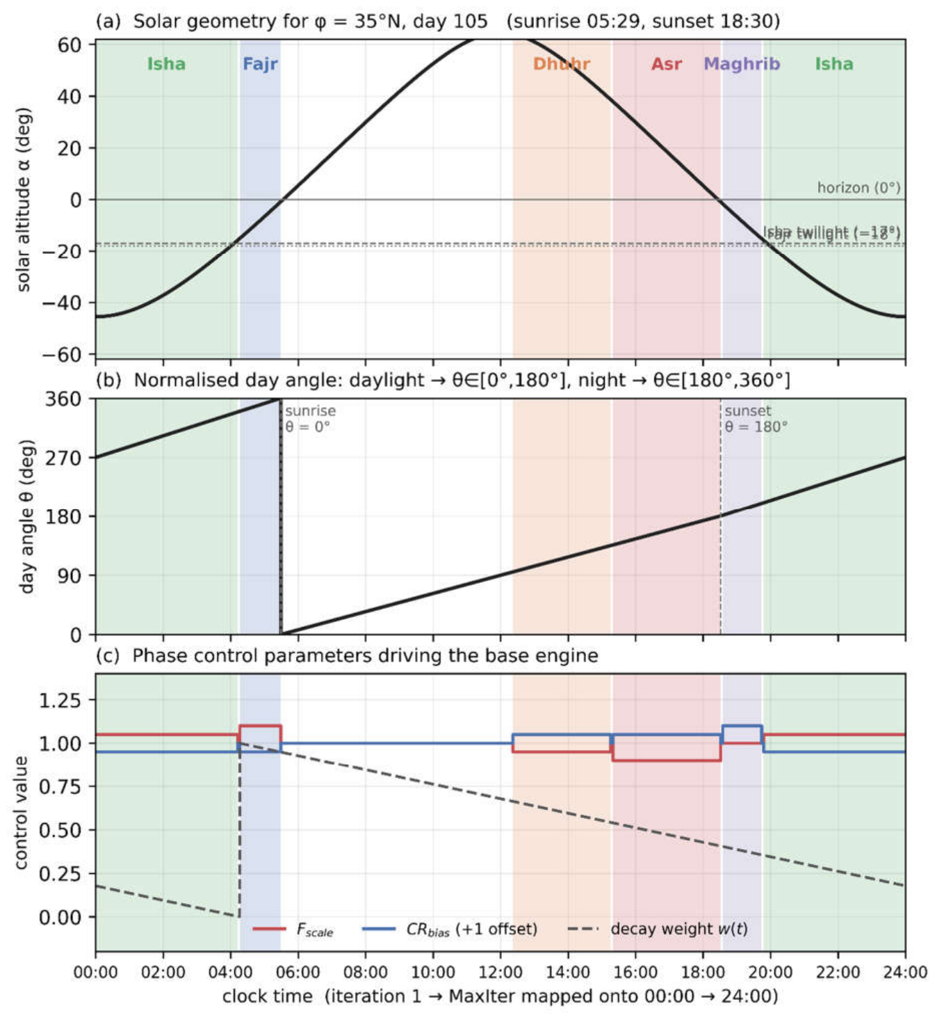
Figure 5.
The five phase operators and the solar geometry that generates them, for φ = 35°N on day 105. (a) Solar altitude over 24 hours, with the five prayer windows shaded and the twilight thresholds that define Fajr and Isha marked; the black triangles are the exact prayer instants of Table 3. (b) The day angle θ of Eq. (10)–(11), which maps daylight onto [0°, 180°] and night onto [180°, 360°]. (c) The control parameters that the active phase applies to the base engine. Generated by Figure 2_pao_phases.m; passing a different latitude or day of year regenerates the whole schedule.
Figure 5.
The five phase operators and the solar geometry that generates them, for φ = 35°N on day 105. (a) Solar altitude over 24 hours, with the five prayer windows shaded and the twilight thresholds that define Fajr and Isha marked; the black triangles are the exact prayer instants of Table 3. (b) The day angle θ of Eq. (10)–(11), which maps daylight onto [0°, 180°] and night onto [180°, 360°]. (c) The control parameters that the active phase applies to the base engine. Generated by Figure 2_pao_phases.m; passing a different latitude or day of year regenerates the whole schedule.
2.9. Modelling Assumptions and the Reference Configuration
The astronomical schedule described above is exact in principle, but the reference implementation realizes it under three simplifications made on purpose. They are stated here so that the results reported later can be reproduced and the scope of the model understood.
First, the Earth’s surface at the observer is idealized as a flat, unobstructed plane. The observer is taken to stand on a level horizon, and no correction is applied for elevation above sea level or for local topography such as the surrounding mountain ranges; the dip of the horizon that arises from the Earth’s curvature and the observer’s height is likewise neglected. This is the standard idealization used in elementary prayer-time computation. It leaves the celestial geometry of Eqs. (1)–(6) unchanged — the Sun’s altitude is still obtained from the standard astronomy formula — and affects only the reference level of the local horizon against which sunrise, sunset, and the twilight angles are measured. In adopting it we set aside the actual elevation of the reference city (Chamchamal lies a few hundred meters above sea level, in a plain flanked by mountains); the resulting shift in the computed instants is small relative to the spread already introduced by the choice of juristic convention, and it does not alter the phase structure that PAO extracts from the schedule (Bahri & Hasibuan, 2024; Meeus, 1991).
Second, a single reference location is fixed for all worked examples and for the default clock of the implementation: the city of Chamchamal, in Sulaymaniyah Governorate, Kurdistan Region, Iraq, at approximately . This latitude is deliberately close to the used in the worked example of Section 2.7, so that the validation figures reported there correspond to the reference city itself. Because the schedule takes latitude and day of year as its only inputs, however, nothing in the method depends on this choice: substituting the coordinates of any other location, or any other date, regenerates a complete and equally valid schedule at no additional tuning cost (see Figure 4).
Third, among the four Sunni schools the Shafi’i school of jurisprudence is adopted throughout. In practice this fixes a single quantity, the shadow factor of the afternoon prayer: the Shafi’i criterion corresponds to in Eq. (10), so ʿAṣr begins when the shadow of an upright object exceeds its noon length by one object-height. The Hanafi value k = 2 would move only the ʿAṣr boundary and would leave the four remaining phases, and the overall exploration–exploitation profile of the schedule, unchanged. For Fajr and Isha the twilight depressions of and stated in Table 3 are used, consistent with the conventions commonly applied at this latitude (Rojak & Fawzi, 2024).
Figure 7.
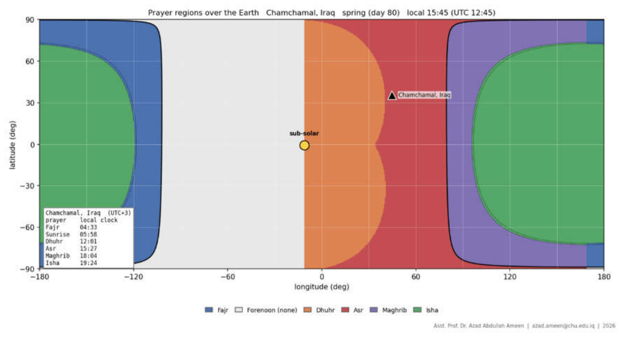
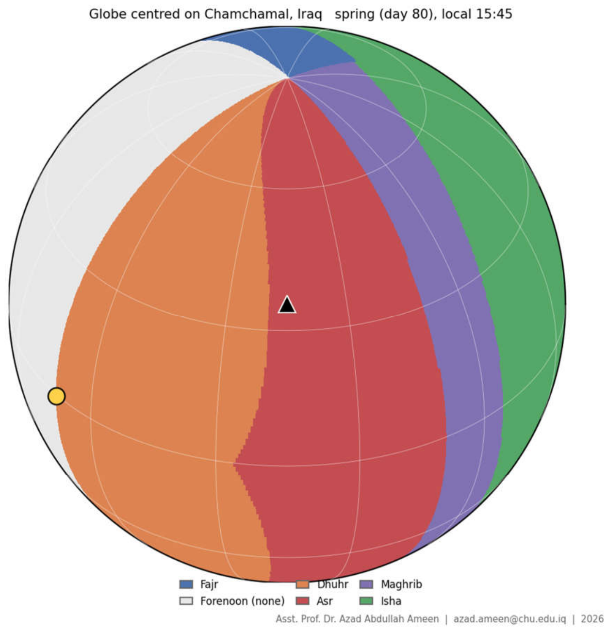
The prayer schedule projected onto the whole Earth at a single instant, for the Chamchamal reference configuration (spring, day 80, local 15:45). (a) Equirectangular map and (b) orthographic globe centered on Chamchamal; each color marks the region of the Earth in which a given prayer is in force at that moment, with the sub-solar point (yellow disc) and Chamchamal (triangle) marked. The figure makes concrete why the schedule must depend on latitude, longitude and date: at one instant different places sit in different prayers, and the local clock times listed in the inset (Fajr 04:33, Sunrise 05:58, Dhuhr 12:01, Asr 15:27, Maghrib 18:04, Isha 19:24) follow directly from the geometry of Section 2 rather than from a stored timetable.
Figure 7.
The prayer schedule projected onto the whole Earth at a single instant, for the Chamchamal reference configuration (spring, day 80, local 15:45). (a) Equirectangular map and (b) orthographic globe centered on Chamchamal; each color marks the region of the Earth in which a given prayer is in force at that moment, with the sub-solar point (yellow disc) and Chamchamal (triangle) marked. The figure makes concrete why the schedule must depend on latitude, longitude and date: at one instant different places sit in different prayers, and the local clock times listed in the inset (Fajr 04:33, Sunrise 05:58, Dhuhr 12:01, Asr 15:27, Maghrib 18:04, Isha 19:24) follow directly from the geometry of Section 2 rather than from a stored timetable.
3. The Proposed PAO Algorithm
This section turns the idea of Section 2 into a working method. It maps a complete run of the algorithm onto a single day, so that each iteration falls at a particular clock time and therefore inside one of the five prayer windows. Each window switches on its own search behavior: Fajr restarts the worst solutions, Dhuhr pulls the group together, Asr makes small careful improvements, Maghrib moves strongly toward the best solution found so far, and Isha gives stuck solutions a large jump. The section gives the equations for each of these steps, the settings they use, the pseudocode and flowchart of the complete method, and an estimate of how much computing work it needs.
3.1. Problem Statement and Notation
PAO addresses the bound-constrained single-objective minimization problem:
Equation (12) states the optimization problem that PAO addresses: to locate the vector x that minimizes the objective function . Here x = (x₁, …, x_d) is a candidate solution composed of d decision variables, ℝ^d denotes the space of real-valued vectors of length , and and are the lower and upper bounds on the variable, so that each coordinate remains within its permitted interval. This is the standard formulation of a bound-constrained minimization problem and is adopted by PAO without modification. Where is treated as a black box: no derivative, no continuity and no convexity is assumed. Table 7 lists the symbols used throughout.
3.2. How PAO is Put Together
PAO has two layers, and it is important to be clear about which is which:
The lower layer is the base engine: an adaptive, population-based search engine that mutates each candidate using a scaled difference between population members, keeps a small external archive of replaced solutions, and self-tunes its own step size and mixing rate as the run proceeds. It is a well-known, off-the-shelf method that we do not claim as new; it runs on every iteration and does most of the search.
The upper layer is the astronomical controller, and this is what PAO contributes. On each iteration it converts the iteration counter into a position in the solar cycle, decides which of the five prayer windows that position falls in, and then does two things: it multiplies the engine’s two control parameters by phase-specific factors, and it switches on at most one additional operator chosen to suit the character of that window. When the position falls in the forenoon gap, no additional operator runs at all.
3.3. Initialization
The starting solutions are scattered evenly, at random, across the whole search region — each coordinate is set to with drawn uniformly from — and the best individual is recorded.
The two success-memories — the small tables that remember which step-size and mixing settings have worked well recently — are set to , the archive — the running store of parents that have just been replaced — starts empty, and the counter that records how long each individual has gone without improving is reset to zero. The daily prayer-time schedule of Section 2 is worked out once before the loop, because it depends only on the latitude and the day of the year .
3.4. The Base Engine
The lower layer is the adaptive, population-based base engine described in Section 3.2. Because it is established machinery and not part of the contribution, only it’s one characteristic step is written out; the remaining textbook steps are described in words. On each iteration, for every individual, the engine samples a scale factor F and a crossover rate from two small memories of recently successful values — from a heavy-tailed random draw (a Cauchy distribution), from a normal, bell-curve draw — and then shifts them by the phase multipliers and supplied by the controller of Section 3.5, which is the only point at which the controller reaches into the engine. The new trial solution combines the current solution with a move toward one of the best individuals and a scaled difference between a population member and a partner drawn from the population together with the archive:
Here is one of the current best individuals, selected at random from the top-ranked fraction; is a randomly chosen population member; is a member drawn at random from the union of the population and the external archive of recently replaced solutions; and is the individual scaling factor. The base engine of Section 3.4 supplies this operator; PAO leaves its form unchanged and only rescales according to the active phase.
The trial is then mixed with the parent coordinate by coordinate, always keeping at least one coordinate from the trial so it can never be an exact copy; the trial is brought back inside the box and replaces the parent only when it is at least as good. Every replaced parent is kept in an external archive of capacity , and at the end of each iteration the two memories are refreshed from the and values that produced improvements, each weighted by how much it improved the objective ((a special average that leans toward the larger successful values, for , a weighted average for ). These are all standard steps of the base engine and are not written out here.
The slot index advances by one each iteration and wraps around at , so the memories hold a moving record of what has recently worked.
3.5. The Astronomical Controller
The run is mapped onto one solar day. Iteration it is placed at:
Equation (14) maps the iteration index onto a time of day, so that the prayer schedule can govern the search. Here it is the current iteration, is the total number of iterations, 1440 is the number of minutes in a day, and ⌊·⌋ denotes the floor (round-down) operation. Consequently, the first iteration corresponds to 00:00 and the final iteration to approximately 24:00. This mapping is introduced in the present work and is the mechanism by which the astronomical schedule is connected to the optimizer.
The day angle follows from . Comparing with the windows of Table 4 selects the phase. A weight that falls linearly from one to zero across the cycle, measured from the start of Fajr, controls how strongly the phase operators act:
Equation (15) defines the cycle weight , a quantity that decreases from one to zero and indicates how far the run has advanced through the day. Here is the time obtained from Equation (14), is the start time of Fajr, the modulo-1440 operation wraps the elapsed time around the 24-hour clock, and division by 1440 scales the result to the interval [0, 1]. The weight therefore equals one at Fajr and decreases linearly to zero across the cycle. It is a design choice for the present work: the schedule is read from the solar day rather than from a fixed decay curve.
Operators that should be strong early use directly; the one that should strengthen late uses . Table 8 collects the phase settings.
3.6. Fajr — Opposition-Based Re-Seeding
Fajr occupies the darkest part of the cycle, just before first light, and its role is exploration. The worst of the population are reflected through the center of the search box to the point directly opposite, and the reflection is kept only if it is better:
Here is the opposite (mirror) point of , and the reflected point is retained only if it improves the objective, ; otherwise is left unchanged.
This is opposition-based learning restricted to the individuals that have least to lose. It costs one evaluation per re-seeded individual and can move a solution across the entire domain in a single step, which no differential mutation can do once the population has contracted.
3.7. Dhuhr — Median Pull
Dhuhr begins just after the Sun crosses the meridian, when shadows are shortest. Its role is contraction, but toward the population itself rather than toward the current best. Let be the coordinate-wise median of the population. A random 30% of individuals are drawn part of the way toward it:
Here m is the coordinate-wise median of the population (a central value that is unaffected by extreme points), is a uniform random number in [0, 1], and = controls the step length, which diminishes as the day advances.
Moving toward the middle of the group rather than toward the best solution is what makes this a balancing step instead of a second exploitation step. The middle value is not affected much by a few unusual points, so the operator draws the population closer together without locking it onto whichever region currently holds the best solution.
3.8. Asr — Local Gaussian Refinement
Asr is defined by shadows lengthening past a fixed multiple of the object height, and it is the exploitation phase. A random 35% of individuals take a Gaussian step whose width in each coordinate is proportional to how far that coordinate currently sits from the best solution:
Here is a standard normal random variable generated independently for each coordinate, ⊙ denotes the coordinate-wise (elementwise) product, is the per-coordinate distance from to the best solution found so far , so that individuals near take small steps and distant individuals take larger ones, and sets the overall magnitude. The candidate is accepted only if it improves the objective.
Scaling the step by the distance to the best gives the operator a useful property: individuals already close to take small steps and fine-tune, while distant individuals take larger ones and do not get stuck. The step size needs no separate schedule because the population supplies it.
3.9. Maghrib — Greedy Attraction
Maghrib is the shortest window, a boundary event at sunset. It is the most directly exploitative operator: a random 30% of the population move a fraction of the way toward the best solution found so far, keeping the move only if it helps:
Here is the best solution to date, is a uniform random number in [0, 1], and increases as decreases, so that the attraction is strongest near the end of the run. The candidate is accepted only if it improves the objective.
Because is built from rather than , this is the one operator that grows stronger as the run proceeds, which is the conventional behaviour and is placed here deliberately: it is the last intensification before the exploratory Isha phase takes over.
3.10. Isha — Lévy Restart
Isha is the longest window, covering about the final third of the run, and its role is recovery of diversity. Any individual whose stagnation counter has reached the threshold = is displaced by a heavy-tailed Lévy step scaled to the width of the box:
Here is a Lévy-flight step—predominantly small but occasionally very large—with stability index , generated by Mantegna’s method; the coordinate-wise product with () scales the step to the width of the search box; and the factor 0.05 keeps its average magnitude moderate.
An individual that has stopped improving therefore usually stays near where it was and sometimes leaves completely. If no individual has stopped improving, the worst 5% are handled instead, so the operator always does something. The move is kept only on improvement.
Placing an exploratory operator last is the point at which PAO departs most clearly from a usual shrinking-only schedule. A monotonically decreasing coefficient cannot re-expand the search once diversity has been lost; a schedule read off the solar cycle can, because the Sun sets as reliably as it rises.
3.11. Boundary Handling
Every candidate produced by any operator is brought back inside the allowed range by clamping (see section3.4): a coordinate that has left the interval is set to the nearest limit it went past. Clamping is fast and never fails, but it piles points up right on the edge, which is itself a known source of built-in search bias. Reflection back into the interior is the usual alternative and is worth testing as part of the sensitivity study.
3.12. Exploration, Exploitation, and the Balance Between them
Table 9 classifies the operators. Two features of the ordering matter. First, the phases run exploration, neutral, balancing, exploitation, exploitation, exploration across the cycle, so the sequence is not monotone. Second, the exploration phase is the last and the longest, which means diversity lost during Asr and Maghrib can be regained before the run ends.
To report the balance with numbers rather than by simply claiming it, population diversity should be recorded at every iteration and turned into exploration and exploitation percentages using the standard measure: the diversity is the average over the dimensions of the mean distance of the individuals from the population median, the exploration percentage is that diversity as a fraction of its largest value seen so far, and the exploitation percentage is the remainder.
Plotting these two curves against the iteration index, with the five windows shaded as in Figure 2, gives direct evidence for or against the claim that the schedule is non-monotone. This is the figure to include in Section 5.7, and it is the one a doubtful reviewer will look for first.
3.13. Control Parameters and Sensitivity
Table 10 lists every quantity that a user could change. They fall into three groups: the two that any population method has, the engine parameters inherited from the base algorithm, and the parameters introduced by PAO itself.
Three sensitivity experiments are needed, and each answers a different question. A one-factor-at-a-time test of values around the defaults, thirty runs per setting, establishes which parameters matter. A test that removes one phase operator at a time (an ablation study), replacing it with the base engine alone, establishes whether each operator is worth keeping; without this the paper cannot show that the five-phase structure contributes anything beyond the base engine underneath. Testing a range of and n values shows whether the schedule family matters at all, and it is the experiment most specific to this algorithm: if performance does not change with φ and n, the astronomy is just for show and would have to be justified some other way.
One point should be given upped rather than left for a referee to raise. Counted fairly, PAO carries more than five primary control parameters, which places it in the highest-parameter category of the parameter-count taxonomy used in Section 1. Fewer parameters are preferable for industrial use, and the natural response is to consolidate: the four subset fractions could share one value, and the three strength coefficients could be expressed as one coefficient times a fixed per-phase ratio. If the sensitivity study shows that doing so costs little, the consolidated version is the one to present.
3.14. Computational Complexity and Evaluation Accounting
Per iteration the engine performs O(N d) arithmetic for mutation and crossover and O(N log N) for the ranking that supplies the set; each extra operator adds O(k d) for the k individuals it touches. The solar schedule is computed once. Over a whole run,
Equation (21) states the time complexity of a single run. Here O denotes asymptotic order, is the number of iterations, N is the population size, is the number of variables, and accounts for the ranking required to identify the best individuals. The total cost therefore is scaled with the product of the iteration count, the population size, and the sum of the dimension and a small ranking term; it grows linearly in both population size and dimension, as is typical for this class of algorithms.
Objective evaluations are the quantity that must be controlled for a fair comparison, and they are not constant per iteration. The base engine spends , and the active phase spends the amount listed in the last column of Table 9. Scaling those costs by the window shares of Table 4 gives an expected:
Equation (22) accounts for the number of objective-function evaluations performed per iteration, which exceeds because the phase operators introduce additional evaluations. Here denotes the expected (average) value, denotes function evaluations, and N is the population size. The base search performs evaluations per iteration, and the phase operators add a further amount, yielding approximately 1.12 on average, or about 12% more. The figure is obtained by weighing each operator’s cost by the frequency with which its phase is active (Table 4); it is the reason a fair comparison must terminate on an evaluation budget rather than on an iteration count.
So, each iteration costs about 12% more than N evaluations. To keep the comparison fair, the corrected code stops on a fixed evaluation budget · rather than on the iteration count, so PAO spends the same number of evaluations as its competitors and simply runs proportionally fewer iterations.
3.15. Pseudocode
Figure 5. illustrate the Pseudocode of Pray Algorithm Optimization (PAO).

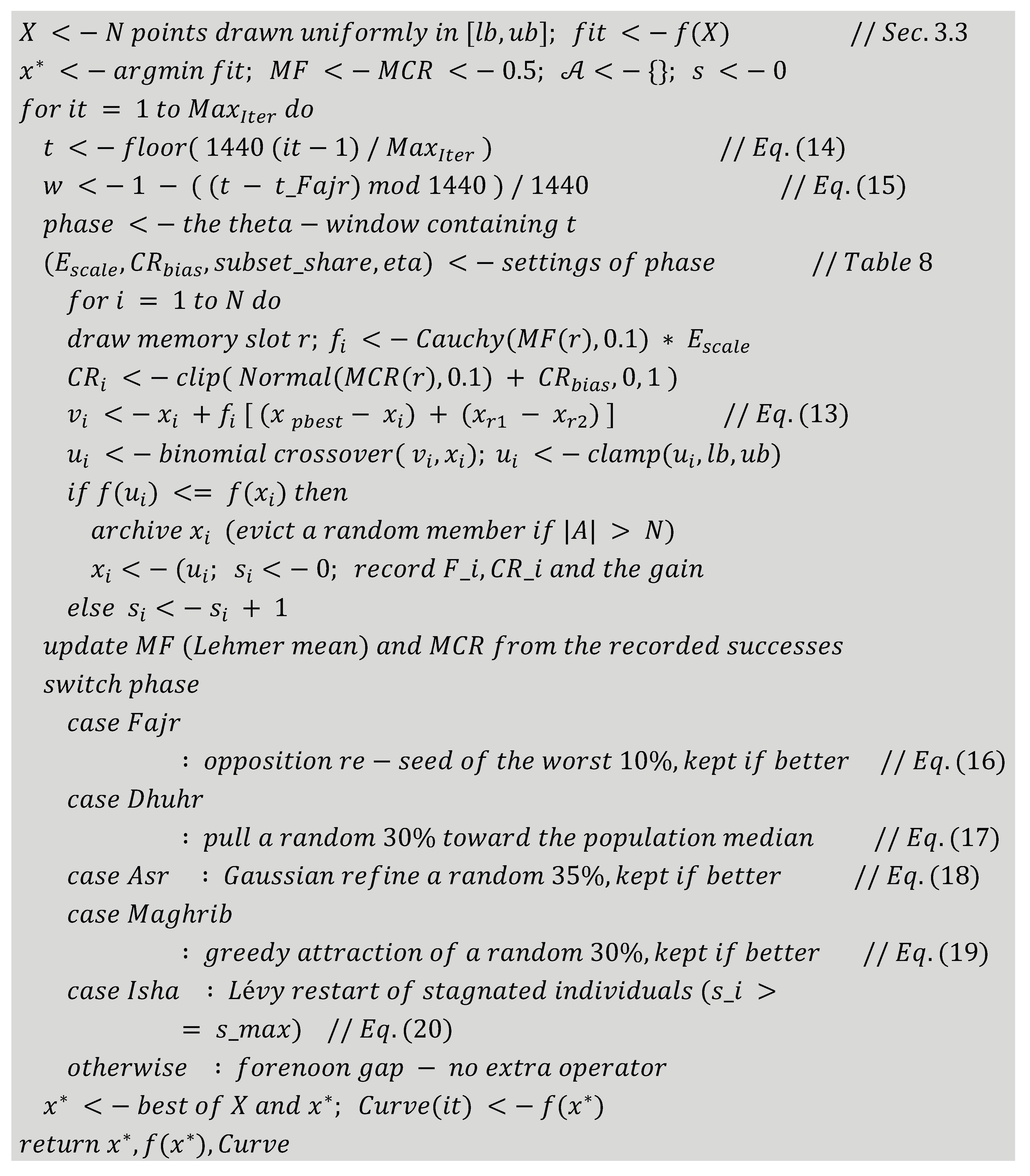
Every step map onto one box of the flowchart in Figure 3. The switch at lines 21 to 27 is the six-way branch; note that exactly one branch runs per iteration, so the operators never compound within a single generation.
Figure 8.
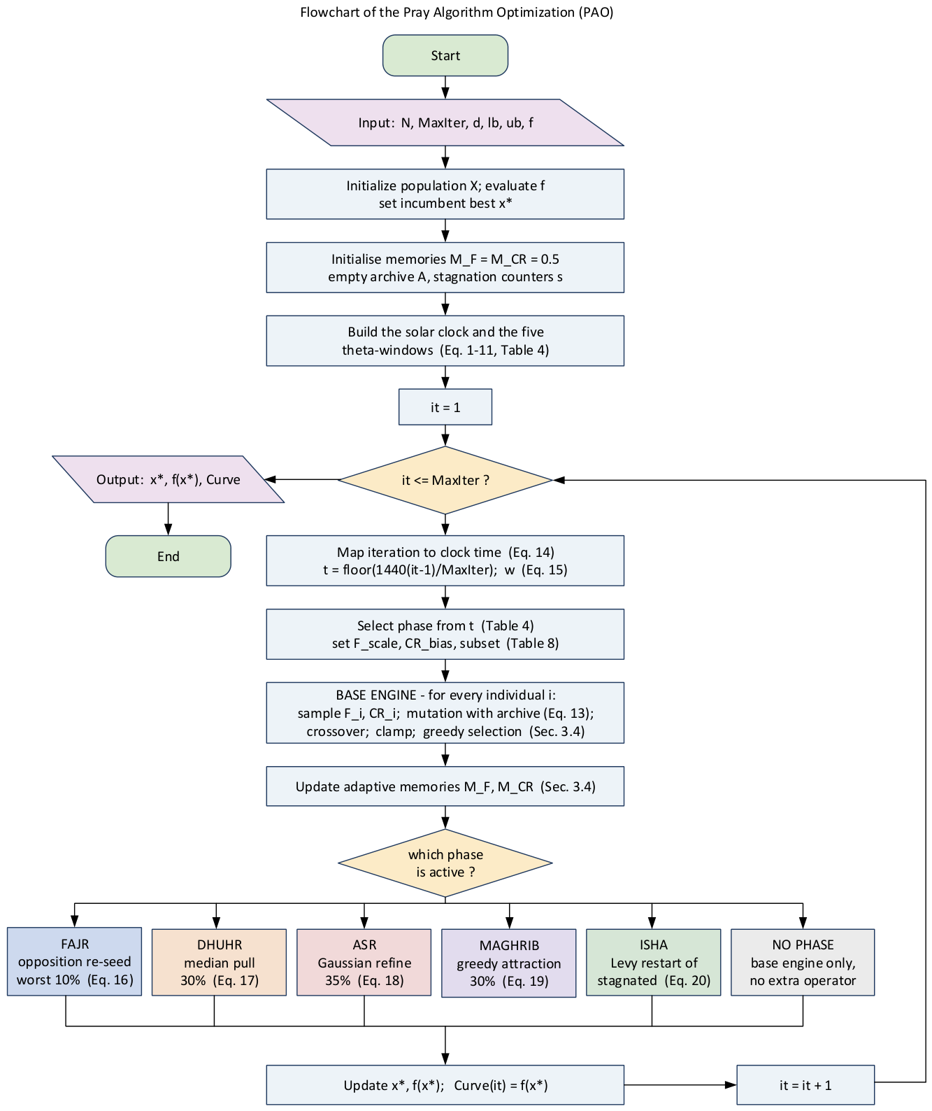
Flowchart of PAO. The solar schedule is computed once before the loop because it depends only on φ and n. Inside the loop the base engine runs every time, without any test and the phase selector activates at most one of the five operators, or none during the forenoon window.
Figure 8.
Flowchart of PAO. The solar schedule is computed once before the loop because it depends only on φ and n. Inside the loop the base engine runs every time, without any test and the phase selector activates at most one of the five operators, or none during the forenoon window.
3.16. Algorithmic Novelty Related to PSO, DE, GWO, SCA
Because PAO’s lower layer is an established adaptive base engine (Section 3.2), the case for novelty rests on the astronomical controller and the five phase operators it activates, not on the search engine underneath. This subsection makes that case explicit by contrasting PAO with four widely used metaheuristics — particle swarm optimization (PSO), differential evolution (DE), the grey wolf optimizer (GWO), and the sine–cosine algorithm (SCA) — each chosen because it embodies one of the mechanisms PAO might be mistaken for. The comparison is organized around the single feature that separates PAO from all four: how the balance between exploration and exploitation is scheduled over a run.
PSO moves every particle by one velocity rule that blends inertia with attraction toward the particle’s own best position and the swarm’s global best (Kennedy & Eberhart, 1995). The rule is homogeneous — the same update acts on every particle at every iteration — and its exploration–exploitation balance is governed by an inertia weight that is almost always driven down a fixed, monotone schedule. PAO differs on both counts. It does not apply one rule uniformly: it selects, from five operators, the one suited to the current solar window, and it leaves a forenoon interval in which no extra operator runs at all. And its balance is not a monotone decay but a non-monotone solar profile in which an exploratory phase (Isha) returns at the end of the run. The one point of contact — Maghrib’s greedy attraction toward the incumbent best — resembles PSO’s social pull, but in PAO it acts on a random subset during a single short phase rather than on the whole population throughout.
DE searches by mutating each solution with a scaled difference between population members and then keeping the better of the parent and the trial; its exploration–exploitation balance is carried by a scale factor and a crossover rate, which in adaptive versions are tuned from recent successes, while any population-size reduction it applies decreases monotonically (Storn & Price, 1997). The contrast with PAO is the same in kind as for the other three comparators. DE applies one mutation-and-crossover rule uniformly across the whole run, whereas PAO overlays an external controller that (i) rescales the engine’s step size and mixing rate by phase-specific factors drawn from the solar schedule rather than from search history alone, and (ii) activates, in different windows, five operators that a bare mutation-and-crossover scheme does not contain: opposition-based re-seeding, a pull toward the population median, distance-scaled Gaussian refinement, greedy attraction to the best, and a heavy-tailed Lévy restart of stagnated individuals. Because that operator layer is what is switched on and off, an ablation that disables it returns PAO to its base engine, which is how the paper isolates the contribution.
GWO steers each search agent toward the three highest-ranked agents, with a coefficient vector that decreases linearly from two to zero across the run; this single decay is the whole of its exploration-to-exploitation mechanism (Mirjalili et al., 2014). The contrast is the same in kind as with PSO but sharper: GWO’s control is one hand-set, monotone linear schedule, whereas PAO’s is a non-monotone schedule computed from solar geometry with no fitted constant. GWO applies leadership-following on every iteration; PAO applies qualitatively different operators in different windows. The resemblance is again narrow — Maghrib’s attraction to the single incumbent best echoes GWO’s pull toward its leaders — but it is confined to one phase rather than being the algorithm’s sole engine.
SCA is the most instructive comparison, because it too drives its search with a smooth periodic function: positions are updated through sine and cosine terms whose amplitude, set by a parameter r₁, decreases linearly toward zero over the run (Mirjalili, 2016). Superficially this is very close to PAO’s use of a trigonometric solar signal. Three differences separate them. First, SCA’s amplitude decays monotonically, so it’s swinging up and down shrinks and the method becomes purely exploitative late in the run, whereas PAO’s driving quantity — the shadow ratio, which behaves like cot α — is non-monotone and grows again toward the ends of the cycle, so exploration recovers. Second, SCA’s periodicity is an abstract oscillation whose range depends on a free coefficient that must be chosen, while PAO’s periodicity is the real solar cycle, fixed completely by latitude and day of year, so the schedule carries no constant for the designer to tune. Third, SCA applies one homogeneous sine–cosine update throughout, whereas PAO uses its periodic signal only to partition the run into phases, each of which then runs its own operator.
Two clarifications follow from these comparisons, and both matter how the contribution should be judged. The individual operators PAO switches among are not themselves new — opposition-based learning, Lévy-flight restarts, Gaussian local search, and greedy selection all predate this work — and neither is the base engine. The novelty lies in their organization: a real astronomical signal, parameterized by nothing but a latitude and a date, is used as an external control schedule that is (a) non-monotone, so that exploration can be regained late rather than only lost; (b) phase-structured, so that distinct operators act in distinct, geometrically defined windows rather than a single rule acting uniformly; and (c) free of any fitted schedule constant, so that changing φ or n produces a whole family of valid schedules at no tuning cost. None of PSO, DE, GWO, or SCA has any of these three properties; their control profiles are all single, monotone, hand-set decays. This is also the sense in which PAO is intended to be strongly rather than weakly inspired, in the terms of Section 1.4: the solar geometry is computed from its governing equations and actively sets the search behavior, not merely named after the fact (Aranha et al., 2022; Sörensen, 2015). Table 11 summarizes the comparison of the four axes that define PAO’s contribution.
4. Experimental Setup
This section describes how PAO was tested, so that the study in Section 5 can be reproduced in full. It specifies the four collections of benchmark problems (see section 4.1), the 42 competing algorithms and the control-parameter values taken from their original publications (see section 4.2), and the protocol that keeps the comparison fair — an identical population size, an identical budget of function evaluations, and 30 independent runs for every algorithm on every problem (see section 4.3). It then defines the measurements used to summarize the raw results and the rule for ranking tied values (see section 4.4), the statistical tests used to decide whether a difference between two algorithms is real rather than chance (see section 4.5), and the computing environment (see section 4.6). The design follows the reproducibility conventions now standard in the metaheuristic literature (Derrac et al., 2011; LaTorre et al., 2021), so that every claim made later can be re-derived from the settings given here.
4.1. Benchmark Suites
PAO is evaluated on four complementary collections — one classical and three from the IEEE CEC competition series — chosen so that the test set is neither dominated by easy separable problems nor by any single generation of difficulty.
Classical set (F1–F23): The 23 functions of (Yao et al., 1999), used throughout the swarm-intelligence literature, are included for comparability with earlier work. They fall into three groups: F1–F7 are unimodal (a single optimum) and probe exploitation and convergence speed; F8–F13 are high-dimensional multimodal (a number of local minima that grows with dimension) and probe exploration and the ability to escape local optima; F14–F23 are fixed-, low-dimensional multimodal (2–6 variables, few minima) and probe the exploration–exploitation balance on small landscapes. F1–F13 are scalable and are run at dimension D = 30 (the conventional setting); F14–F23 keep their native dimensions. The search bounds and the known optimum of each function are listed(Yao et al., 1999) in Table A7.
CEC2017 (Pham et al., 2023): Thirty shifted-and-rotated functions are defined; following the common convention the second function (F2) is omitted because its values are numerically unstable across implementations, leaving 29 functions. They comprise 2 unimodal (F1, F3), 7 simple multimodal (F4–F10), 10 hybrid (F11–F20) and 10 composition (F21–F30) problems on the box [−100, 100] in each of D dimensions, with known optima . The suite is run at D ∈ {10, 30, 50, 100} to expose scaling behavior. The hybrid and composition functions, which glue several rotated sub-functions together, are the ones on which purely exploitative methods stop making progress — exactly the regime the non-monotone schedule of Section 3 is meant to address (see Table B7).
CEC2019 — the “100-Digit Challenge” (Hamid et al., 2026; Price et al., 2018): Ten functions (CEC01–CEC10). The first three carry their own dimensions (CEC01: 9-D, CEC02: 16-D, CEC03: 18-D); CEC04–CEC10 are all 10-D. Every function is shifted and rotated and has a global minimum value of 1, so results are reported as the gap above 1. The suite is deliberately small in dimension but severely ill-conditioned, which stresses fine-grained exploitation late in a run (see Table C7).
CEC2022 ((Salgotra et al., 2025)): Twelve functions on [−100, 100] in each of D dimensions at D ∈ {10, 20}: 1 unimodal (F1), 4 basic multimodal (F2–F5), 3 hybrid (F6–F8) and 4 compositions (F9–F12). As the most recent suite, it provides an up-to-date and widely reported benchmark (see Table D7).
Together the four suites span separable and non-separable, unimodal and multimodal, low- and high-dimensional, and shifted/rotated/hybrid/composition landscapes, giving a total of well over seventy distinct problem instances once dimensions are counted separately.
4.2. Comparator Algorithms, Parameters, Complexity and Budget
PAO is compared against the 42 algorithms of the taxonomy in Figure 1 (listed in Table 2), which together represent the evolutionary, swarm-intelligence, physical-law-based and miscellaneous families. Every comparator is run with the control-parameter values recommended in its original publication; none is re-tuned for the present problems. Re-tuning only PAO, or only its competitors, is the most common source of biased comparisons, so all algorithms are used “as published” and PAO itself is run with the single default configuration of Table 10 on every problem, with no per-suite tuning.
4.3. Fairness Protocol
Three settings are held identical for every algorithm on every problem, so that any observed difference is attributable to the search behavior and not to the resources granted:
- (1)
- Identical population size. All algorithms use the same N (reported with the results; N = 60 unless a suite’s official protocol prescribes otherwise).
- (2)
- Identical evaluation budget. Every run terminates when it has consumed MaxFEs = N · objective-function evaluations, not when it reaches a fixed iteration count. Evaluations are counted individually inside every algorithm, including PAO’s phase operators, which spend extra evaluations per iteration (Section 3.14). Stopping on MaxFEs therefore removes the roughly 12% budget advantage that an iteration-based stop would otherwise give PAO and gives every comparator the same number of chances to improve. The value of MaxFEs used for each suite is reported with the results.
- (3)
- Thirty independent runs. Each (algorithm, function, dimension) triple is solved in 30 independent runs with independent random seeds, so that the reported statistics reflect the distribution of outcomes rather than a single lucky or unlucky trajectory.
In addition, all algorithms share the same box constraints and the same uniform-random initialization within the feasible region, no algorithm is given the location or value of the optimum, and all bound-handling is by the saturation rule of Section 3.11. The complete list of per-suite N and MaxFEs values is given in Appendix A.
4.4. Performance Metrics and the Tied-Rank Method
For each (algorithm, function, dimension) the 30 final best-so-far objective values are reduced to five statistics: the mean, the standard deviation, the best, the worst, and the median. The mean ± standard deviation is the primary quality/robustness pair; the median, best and worst guard against a mean distorted by a single outlier run and expose skew.
To summarize performance across functions, algorithms are converted to ranks. On each function the algorithms are ordered from best () to worst () by their mean value (with the median used to break exact mean ties). Tied results are given the average of the ranks they span — for example, two algorithms tied for positions 3 and 4 both receive rank 3.5 — so that the ranks on every function still sum to and no algorithm is arbitrarily favoured by the ordering of ties. Each algorithm’s average rank over all functions is then the single number used to compare methods and to build the diagrams of section 4.5. This tied-rank convention is the one required by the Friedman procedure and is what makes the rank-based tests below valid.
4.5. Statistical Tests
Raw means can differ by amounts too small to be meaningful, so all conclusions in Section 5 are supported by non-parametric statistics, which make no normality assumption about the 30-run samples (Derrac et al., 2011).
Wilcoxon rank-sum test (pairwise): For every function, PAO’s 30 results are compared with each competitor’s 30 results using the two-sided Wilcoxon rank-sum (Mann–Whitney U) test at the significance level. Each comparison is scored as a win (+), tie (=) or loss (−) for PAO, and the overall +/=/− tally against each algorithm is reported.
Friedman test (multiple comparison): The average ranks of section 4.4 are tested with the Friedman test, whose null hypothesis is that all algorithms have equal average rank. The Friedman statistic, its p-value and the resulting ranking are reported; a small p-value licenses the post-hoc analysis.
Post-hoc analysis: When Friedman rejects the null, a Holm step-down procedure (with PAO as the control method) identifies which competitors PAO significantly out- or under-performs while controlling the family-wise error rate across the many pairwise comparisons; the adjusted p-values are reported.
Critical-difference (CD) diagrams: Following (Demšar, 2006) average ranks are drawn on a single axis with a critical difference bar, )CD = where k is the number of algorithms and N꜀ the number of functions. Algorithms whose average ranks differ by less than CD are joined by a bar and are statistically indistinguishable; those not joined differ significantly. The CD diagram gives an at-a-glance summary of the whole comparison and is the figure a reviewer is most likely to inspect first .
Where a suite is run at several dimensions, the tests are applied separately per dimension and then on the pooled ranks, so that both dimension-specific and overall conclusions are supported.
4.6. Computing Environment
All algorithms, including PAO, are implemented in MATLAB [R2020a] and run on the same machine — processor: Intel Core i7-10700 @ 2.90 GHz, 8 cores; Memory: 32 GB RAM; operating system: Microsoft Windows 11 pro — under identical conditions, with each run executed on a single core and no parallelism across runs, so that the wall-clock times used to validate the complexity analysis of section 3.14 are comparable. Reported run-times are the average over the 30 runs. The PAO source code and the scripts that regenerate every table and figure are available at [ https://www.mathworks.com/matlabcentral/fileexchange/184442-pao-for-global-and-constrained-engineering-optimization ].
5. Results and Discussion on Benchmark Functions
This section reports how PAO performed on the four collections of standard test problems. For each collection it gives the average result of every algorithm, ranks them, and reports whether PAO’s advantage is statistically significant. It then looks at the results from several angles: convergence curves, boxplots of run-to-run consistency, the shifting balance between searching and refining, and tests of how the method behaves when the problem gets larger, when the population size changes, and how much time it takes. Where PAO loses, the section says so and explains why.
5.1. Classical Benchmark Functions_23 Functions
This section evaluates the Pray Algorithm Optimization (PAO) against a large contemporary pool of forty-three metaheuristics on the classical set of twenty-three benchmark functions (F1–F23). Performance on every function is the mean fitness over the 30 runs. Per-function ranks were then assigned in ascending order of mean fitness (rank 1 = best), with ties resolved by the standard fractional (mid-rank) convention, and each algorithm’s overall standing was taken as its mean rank across the 23 functions. All supporting numbers are collected in Appendix A.
Averaged over the 23 functions, PAO attains a mean rank of 13.152, placing it second of the 43 algorithms. It is bettered only by SOA, whose mean rank of 11.261 heads the field, and it leads a close chasing group formed by WAA (13.870, 3rd) and DHOLE (14.630, 4th). The Friedman overall test confirms that these rank differences are not attributable to chance (χ² = 311.91, , so the ordering in Table A1 is statistically meaningful rather than an artefact of sampling. PAO can therefore be described, without embellishment, as a strong second-best optimizer on this suite — highly competitive with the leader but not its equal on the combined measure.
The Wilcoxon rank-sum test (α = 0.05) applied function-by-function paints a consistent picture. Added together over all 42 competitors and 23 functions, PAO records 641 wins, 42 ties and 283 losses — a 66.4%-win rate (Table A4). Resolved competitor by competitor, PAO holds a winning record against 33 of the 42 competitors, an even record against 2 (AO and EMRA), and a losing record against only 7. Those seven are SOA and CSA (both 9–14 against PAO), followed by GOA, DHOLE, TSO, SO and HBA, each of which edges PAO by only one or two functions. In other words, exactly one algorithm (SOA) both out-ranks PAO on the mean-rank metric and beats it head-to-head by a clear margin; PAO’s runner-up position is thus robust to the choice of statistical lens.
PAO’s strongest placements are the harder fixed-dimension multimodal landscapes, where it ranks first or near-first on F18, F21, F22 and F23; the per-function ranks are given in Appendix A.
On the easy functions a large fraction of the 43 algorithms drive the mean fitness exactly onto the global optimum — that is, all 30 of their runs converge to the optimal value — so their mean finesses are numerically identical. Under the fractional-ranking rule, a block of k algorithms sharing the best mean does not occupy ranks 1 through k; every member is instead assigned the single averaged rank (k+1)/2. The optimum therefore collapses a whole span of ranks into one value. The effect is severe on this suite (Table A2): the top block contains 18 algorithms on F11 (each assigned rank 9.5), 17 on F9 and again 17 on F16 (rank 9.0), 16 on F10 (rank 8.5), 15 on F19 (rank 8.0), 14 on F17 (rank 7.5), 10 on F14 (rank 5.5) and 8 on each of F1–F4 (rank 4.5). A direct consequence is a loss of resolution in the mean-rank metric itself: on F11, for example, the ranking cannot distinguish the best optimizer from the eighteenth-best, because all eighteen are recorded at 9.5. The between algorithm variance on such functions is largely erased, and the aggregate ranking is decided disproportionately by the minority of functions on which ties do not form.
The compression acts on PAO in both directions: on several separable functions its mean sits a hair above the tie block and is displaced below algorithms it effectively matches, while elsewhere the same rule works in its favor. Appendix A gives the per-function figures.
Because so many ranks depend on the optimum, PAO’s aggregate score is convention dependent. Recomputing the mean rank under the optimistic (minimum) and pessimistic (maximum) tie rules bounds PAO between 11.913 and 14.391 (Table A1). Under the pessimistic rule the reported 13.152 is preserved and PAO remains second; under the optimistic rule PAO would be narrowly overtaken by DHOLE (whose min-tie score of 11.826 benefits from its membership in many optimum blocks), dropping PAO to third. SOA, by contrast, remains first under every convention (min-tie 10.130). The second-place finish is thus stable under the standard fractional rule used throughout this study, while the exact second/third boundary is acknowledged to be tie-rule sensitive.
Taken together, PAO’s mean rank of 13.152 is best read as a conservative estimate of its quality: it is lowered by tie compression precisely on the functions PAO solves to optimality and lifted toward first only by its tie-free, outright wins on the harder multimodal problems. SOA edges ahead because it exploits both fronts at once — it wins the separable unimodal functions clearly (its F1 mean reaches 3.89 × 10−²²³) and simultaneously sits inside the multimodal optimum blocks — whereas PAO trades block membership on the easy functions for dominance on the difficult ones. The same tie structure explains a mild non-transitivity in the results: PAO out-ranks GOA, TSO and HBA on the mean-rank metric yet is slightly net-negative against them head-to-head, because averaged ranks and pairwise counts weight the compressed functions differently. The conclusion holds: on the classical 23-function suite PAO is a robust second, its comparative advantage concentrated on multimodal and composite optimization.
5.2. CEC2017 Benchmark Functions_30 Functions
The CEC-2017 suite was run at dimension D = 30 for the same pool of forty-three algorithms, each for 30 independent runs of 500 iterations. Following the standard convention adopted in Section 4.1, the second function (F2) is excluded because its shifted-and-rotated form is numerically unstable across implementations, leaving twenty-nine functions: two unimodal (F1, F3), seven simple multimodal (F4–F10), ten hybrid (F11–F20) and ten compositions (F21–F30). Performance on each function is the solution error f(x) − f* over the 30 runs (the known optima are f*ᵢ = 100i, so lower error is better and zero denotes the optimum located). Ranking follows the convention of Section 5.1; supporting numbers are in Appendix B.
PAO ranks first. Averaged over the 29 functions, PAO attains a mean rank of 2.172, placing it first of the 43 algorithms clearly. The nearest competitors trail well behind — DOA (5.655, 2nd), NDO (5.966, 3rd), PGA (7.034, 4th), EHO (8.586, 5th) and GOA (9.207, 6th) — so PAO’s average rank is better than the runner-up’s by more than three full rank positions. The dominance is repeated in outright wins: PAO ranks first on 19 of the 29 functions, whereas no other algorithm is first on more than three. The Friedman overall test rejects rank equality overwhelmingly (χ² = 949.83, df = 42, p ≈ 8 × 10⁻¹⁷²), so this ordering is not a chance result of sampling. On this suite PAO can be described, without qualification, as the strongest optimizer in the pool.
The two-sided Wilcoxon rank-sum test (α = 0.05), applied function-by-function, tells the same story. Aggregated over all 42 opponents and 29 functions, PAO records 1150 wins, 56 ties and 12 losses — a 94.4%-win rate (Table B4). Resolved opponent-by-opponent, PAO holds a net-positive record against every one of the 42 competitors without exception and sweeps 16 of them 29–0–0. Even the strongest rivals are beaten decisively: DOA, NDO, EHO, PGA and PSO — the only algorithms to take a single function from PAO — still concede it a net advantage of between +20 and +23. In short, no algorithm in the pool out-ranks PAO or holds an even head-to-head record against it; the first-place finish is robust to the choice of statistical lens.
The advantage is broad rather than concentrated: PAO ranks first on both unimodal functions and on six of the seven simple-multimodal functions and leads the hybrid and composition groups. Per-function errors are listed in Appendix B.
Its one clear weakness is F10 (Shifted-and-Rotated Schwefel, rank 14), whose deceptive geometry places the global basin far from the strong local basins and traps PAO’s late refinement; see Appendix B.
The first-place finish here stands in deliberate contrast to PAO’s second place on the Classical-23 suite (Section 5.1), and the two results are consistent once the difference between the suites is understood. On the easy, separable Classical functions many algorithms drive the mean exactly onto the optimum, so their ranks collapse into large ties and the metric loses resolution — an effect that masked PAO’s true accuracy there. The CEC-2017 functions are shifted, rotated, hybridized and composed specifically to defeat this: almost no algorithm reaches the exact optimum, ties at the optimum vanish, and the ranking therefore has full resolution. Under that sharper lens PAO’s genuine search ability is expressed directly. Tellingly, the algorithms that led the Classical suite by sitting inside optimum tie-blocks collapse here — SOA falls from 1st on Classical-23 to 32nd, and CSA to 42nd of 43 — which indicates their Classical lead reflected tie-compression rather than search power. On the harder, more discriminating benchmark, PAO is the clear leader.
Taken together, the mean rank of 2.172, the 19 first-place finishes, the 94.4% pairwise win rate and the net-positive record against all 42 competitors establish PAO as the best-performing optimizer on CEC-2017 at D = 30. Its comparative advantage is concentrated exactly where it was designed to be strong — the multimodal, hybrid and composition landscapes — and its sole material weakness (the Schwefel function F10) is specific and reproducible. Runtime cost is discussed in Section 5.11; on the quality metrics that matter, PAO leads the field.
5.3. CEC2019 Benchmark Functions_10 Functions
The CEC-2019 “100-Digit Challenge” comprises ten functions (CEC01–CEC10) evaluated for the same pool of forty-three algorithms, each for 30 independent runs of 500 iterations. The first three are real-world problems carrying their own dimensions — Storn’s Chebyshev polynomial fitting (9-D), the inverse Hilbert matrix (16-D) and the Lennard-Jones minimum-energy cluster (18-D) — while CEC04–CEC10 are shifted-and-rotated 10-D problems (Rastrigin, Griewank, Weierstrass, modified Schwefel, expanded Schaffer F6, Happy Cat and Ackley). Every function has a global minimum value of 1, so performance is reported as error (the objective gap above 1), for which lower is better. The suite is small in dimension but severely ill-conditioned, which stresses fine-grained exploitation late in a run. Ranking follows Section 5.1; supporting numbers are in Appendix C.
PAO ranks first. Averaged over the ten functions, PAO attains a mean rank of 4.55, placing it first of the 43 algorithms — and by a striking margin, since the runner-up NDO sits at 10.05, more than double PAO’s figure. The next places are tightly grouped closely and far behind: PGA (10.20, 3rd), DOA (10.80, 4th), PSO (10.85, 5th) and GOA (11.50, 6th). The Friedman overall test rejects equal ranking decisively (χ² = 228.86, df = 42, p ≈ 1.5 × 10⁻²⁷). PAO wins here through consistency, not outright wins: first on only three functions (F4, F5, F9) but top-six on eight of ten, while no competitor is uniformly strong — the chasing group clusters near an average rank of ten precisely because each of them is weak on some subset of the functions. PAO’s low average rank is therefore earned by rarely placing poorly.
The two-sided Wilcoxon rank-sum test (α = 0.05), applied function-by-function, confirms the picture. Aggregated over all 42 opponents and ten functions, PAO records 362 wins, 31 ties and 27 losses — an 86.2%-win rate (Table C4) — and holds a net-positive record against every one of the 42 competitors without exception, sweeping 18 of them 10–0–0. The closest rivals still concede ground: HBA, PGA and NDO, the strongest of the field, each finish only +4 in net terms against PAO. No algorithm out-ranks PAO or holds an even head-to-head record against it, so the first-place finish is robust to the choice of statistical lens.
The advantage is concentrated on the shifted-and-rotated 10-D functions: PAO ranks first on Rastrigin, Griewank and Happy Cat, beating all 42 competitors on each. Appendix C gives the per-function detail.
The exceptions are more numerous here than on CEC-2017. PAO is weakest on F6 (Weierstrass, rank 11), whose fractal landscape defeats late-stage refinement, and only mid-pack on the three real-world functions. Appendix C lists them.
The first-place finish reinforces the CEC-2017 result (Section 5.2): on hard, well-conditioned benchmarks that discriminate sharply between algorithms, PAO leads the field. The difference in character — a consistency-driven win here versus a win-almost-everything result on CEC-2017 — reflects the nature of the 100-Digit suite, where the severe conditioning of individual functions means no single algorithm dominates all ten, and the best overall method is the one that is strong across the board. By that measure PAO is the clear winner, just as it is on CEC-2017; the contrast with its masked second place on the easy Classical-23 suite (Section 5.1) is again explained by the absence here of the optimum-tie compression that flattened the Classical ranking.
Taken together, the mean rank of 4.55 — less than half the runner-up’s — the 86.2% pairwise win rate and the net-positive record against all 42 competitors establish PAO as the best-performing optimizer on CEC-2019. Its strength lies on the shifted-and-rotated multimodal functions, and its limitations are specific: the Weierstrass function and the specialized real-world problems. Runtime is discussed in Section 5.11; on the quality metrics that matter, PAO again leads.
5.4. CEC2022 Benchmark Functions_12 Functions
The CEC-2022 suite — the most recent of the four — comprises twelve functions on [−100, 100]: one unimodal (F1, shifted-rotated Zakharov), four basic multimodal (F2–F5: Rosenbrock, expanded Schaffer F6, non-continuous Rastrigin, Levy), three hybrid (F6–F8) and four composition (F9–F12), with known optima f*ᵢ ranging from 300 to 2700. The suite is defined at D ∈ {10, 20}; the results reported here are for D = 10. Performance on each function is the mean solution error f(x) − f* over the runs (lower is better; zero denotes the optimum located), and ranking follows Section 5.1. Supporting numbers are in Appendix D.
PAO ranks first, but narrowly. Averaged over the twelve functions, PAO attains a mean rank of 4.375, the best in the pool — but here the margin is slim. GOA follows at 4.667 and APO at 5.833, so PAO, GOA and APO form a clearly separated leading trio ahead of PGA (8.708) and DOA (9.083). The Friedman overall test confirms that the overall ranking is highly significant (χ² = 378.08, df = 42, p ≈ 1.2 × 10⁻⁵⁵), but the gap between PAO and GOA at the very top is small enough that the two are best regarded as sharing the first tier rather than cleanly separated. PAO takes outright first place on four functions (F1, F4, F5, F6); GOA, APO and DOA each win two.
The two-sided Wilcoxon rank-sum test (α = 0.05) reinforces this reading. Aggregated over all 42 opponents and twelve functions, PAO records 445 wins, 32 ties and 27 losses — an 88.3% win rate (Table D4) — and holds a net-positive record against 41 of the 42 competitors, sweeping 20 of them 12–0–0. The single exception is instructive: against GOA, PAO is exactly level — five wins, two ties and five losses — so although PAO edges GOA on the average rank metric, the two are statistically indistinguishable head-to-head. APO, the third member of the leading trio, is beaten by a clear +4 (7–2–3). PAO is therefore the top-ranked method on this suite, but honestly it shares the summit with GOA rather than standing alone.
PAO is strongest on the unimodal, basic-multimodal and first-hybrid functions, solving Zakharov and Levy to the optimum on every run. Appendix D gives the per-function results.
The exceptions cluster on two families, the worst being Rosenbrock (rank 11), where a narrow curved valley leaves a mean error of 6.81 although the best run reaches the optimum — a consistency shortfall rather than an inability to solve it. Appendix D has the detail.
This is PAO’s third consecutive first-place finish on a modern, discriminating benchmark, after CEC-2017 and CEC-2019, and it reinforces the overall conclusion that PAO is a leading optimizer on hard problems. The narrower margin here — a near-tie with GOA rather than the wide lead seen on CEC-2017 — reflects both the strength of GOA on this particular suite and that CEC-2022 is the newest and, at the top of the field, the most closely contested collection. As on the other CEC suites, the absence of optimum-tie compression means the ranking has full resolution, so PAO’s first place is a genuine reflection of accuracy rather than the artefact that flattened its Classical-23 standing (Section 5.1).
Taken together, the best mean rank in the pool (4.375), the 88.3% pairwise win rate and the net-positive record against 41 of 42 competitors place PAO at the top of the CEC-2022 ranking, with GOA as a statistically level co-leader. PAO’s advantage lies on the unimodal, basic multimodal and hybrid functions — several solved to the optimum on every run — while its limitations are confined to Rosenbrock and two composition functions. Runtime is discussed in Section 5.11; on quality, PAO leads this suite too, if narrowly.
5.5. Convergence and Distribution of Results
5.5.1. Classical-23
Figure 6 traces the mean best-so-far fitness of every algorithm on each of the 23 functions, with PAO highlighted against the field and a logarithmic vertical axis wherever fitness is strictly positive. The curves make PAO’s search dynamics explicit and complement the end-point ranking of Section 5.1.
On the unimodal and scalable functions PAO exhibits a clean, multi-phase descent. An exploratory phase over the first 10–20% of the budget cuts the error by orders of magnitude — on F1 the mean best-so-far falls from 5.10 × 10⁴ at iteration 1 to about 1.75 by iteration 100 — followed by a sustained, near log-linear refinement phase and a late plateau at the optimum (2.97 × 10−¹² by iteration 500). The same signature appears on the steep F5 valley, where the curve descends from 1.80 × 10⁸ to 32.4, and on the highly multimodal F9, where it falls from 4.03 × 10² to 0.895. No oscillation, stagnation spike or divergence is observed on any PAO trace.
On the fixed-dimension multimodal functions PAO locates and settles into the global basin within a few tens of iterations, consistent with its top ranks there: on F23 the curve moves from −1.28 to the optimum −10.54 by roughly iteration 50, with F18, F21 and F22 behaving similarly. The convergence-iteration summary (Table A5) quantifies this: PAO stabilizes very early on the fixed-dimension set (iteration 31 on F16, 25 on F18) yet continues to improve late on the hardest separable functions (iteration 490 on F4, 497 on F8). This combination — early lock-on where the landscape permits, patient progress where it does not — indicates genuine iterative optimization rather than premature convergence.
The strongest exploiters (SOA, CSA) sit on the numerical floor for most of the run. On the separable functions their best-so-far trace hits the floor within the first logged iterations — SOA’s trace on F1, F5 and F9 is already pinned at zero from iteration 1, although its terminal mean on F1 is 3.89 × 10−²²³ — so an iteration-by-iteration curve comparison against these algorithms is uninformative on those functions, and their relative standing there is better read from the terminal accuracy in Table A3. On the harder multimodal and fixed-dimension functions (F8, F14–F23), where all traces are well resolved, PAO’s curve is competitive with, and frequently ahead of, the leading algorithms — the visual counterpart of its first-place ranks on those problems.
Figure 6.
Convergence behavior on the Classical-23 benchmark suite (30-run mean best-so-far, 500 iterations) PAO highlighted against the field.
Figure 6.
Convergence behavior on the Classical-23 benchmark suite (30-run mean best-so-far, 500 iterations) PAO highlighted against the field.
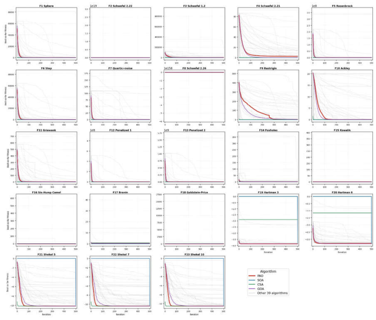
Where the convergence curves describe the typical run, the boxplots in Figure 7 describe the spread across the 30 runs and therefore the robustness of each optimizer. For legibility the panels compare PAO against the eight leading algorithms by mean rank; each box spans the inter-quartile range, the whiskers reach the non-outlier extremes, and individual markers denote outliers, with a logarithmic axis where fitness is positive.
On the functions that drive its ranking — the fixed-dimension multimodal set F16–F23 and the step function F6 — PAO produces tight, low boxes with negligible height, meaning it converges to the same optimum on every run. Its dispersion of these problems matches or improves upon that of the leading algorithms, so PAO’s strong average ranks their rest on repeatable behavior rather than on a few fortunate runs.
On the easy separable functions PAO’s box sits slightly above the leaders and is visibly taller. F9 is the clearest case: PAO’s 30 final values have mean 0.895 and standard deviation 0.990, ranging from a best of 1.85 × 10−⁶ to a worst of 3.98, indicating that a minority of runs settle on a Rastrigin local basin instead of the global optimum. This dispersion is exactly the mechanism identified in Section 5.1: it lifts PAO’s mean just outside the optimum tie block and, through rank compression, drops its rank on those functions. The leaders (SOA, CSA) by contrast show degenerate zero-height boxes on the same problems, every run having reached the optimum.
PAO shows few high outliers, and its whiskers stay close to the box, so even its worst runs are bounded. On most functions the median lies near the center of the box, indicating symmetric run distributions. The boxplots corroborate the ranking of Section 5.1: PAO is highly consistent on multimodal and fixed-dimension problems, and competitively consistent, if slightly more dispersed, on the separable functions where the optimum tie block depresses its rank.
Figure 7.
Distribution of final fitness over 30 independent runs Classical-23 suite PAO versus the eight leading optimizers (lower is better).
Figure 7.
Distribution of final fitness over 30 independent runs Classical-23 suite PAO versus the eight leading optimizers (lower is better).
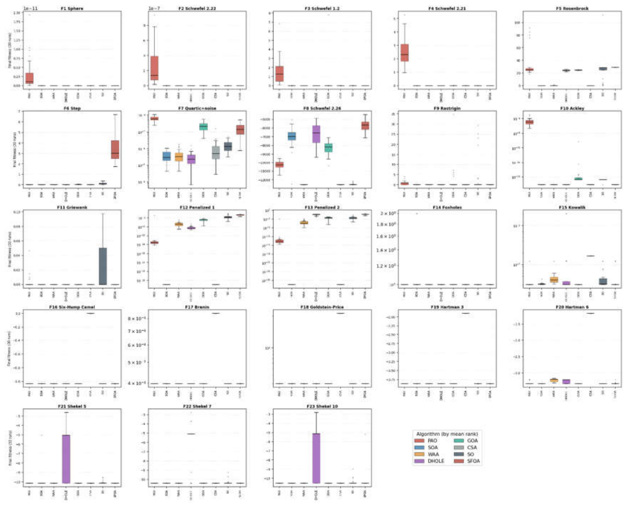
5.5.2. CEC-2017
Figure 8 traces the mean best-so-far error of every algorithm on each of the 29 CEC-2017 functions (F2 omitted), with PAO highlighted and a logarithmic vertical axis.
On the unimodal and simple-multimodal functions PAO shows a steep, multi-order-of-magnitude descent. On F1 the mean error falls from 1.05 × 10¹¹ at iteration 1 to about 1.19 × 10⁷ by iteration 100 and 1.06 × 10³ at the end — roughly eight orders of magnitude — and a similar shape appears on F5 (622 → 18.7) and F11 (3.46 × 10⁴ → 66.9). The trajectory is front-loaded: most of the reduction occurs in the first 100–150 iterations, after which PAO settles into a refinement phase rather than stagnating. No oscillation or divergence is visible on any PAO trace.
On the composition set, PAO descends promptly to the basin floor — F21 moves from 785 to 218 and F23 from 1485 to 368 — and its curve sits at or near the bottom of the field on the large majority of panels, the visual counterpart of its first-place ranks there. The exception is visible too: on F10 the curve descends only modestly (9447 → 4711) and plateaus well above the leaders, which is exactly the rank-14 outcome discussed in Section 5.2. The panels show early, clear progress on almost every function, with the Schwefel function the single case where PAO’s late-stage refinement is out-paced.
Figure 8.
Convergence behavior on the CEC-2017 benchmark suite (30-run mean best-so-far error, 500 iterations, D = 30 Colors as in Figure 6. F2 is omitted per the standard convention.
Figure 8.
Convergence behavior on the CEC-2017 benchmark suite (30-run mean best-so-far error, 500 iterations, D = 30 Colors as in Figure 6. F2 is omitted per the standard convention.
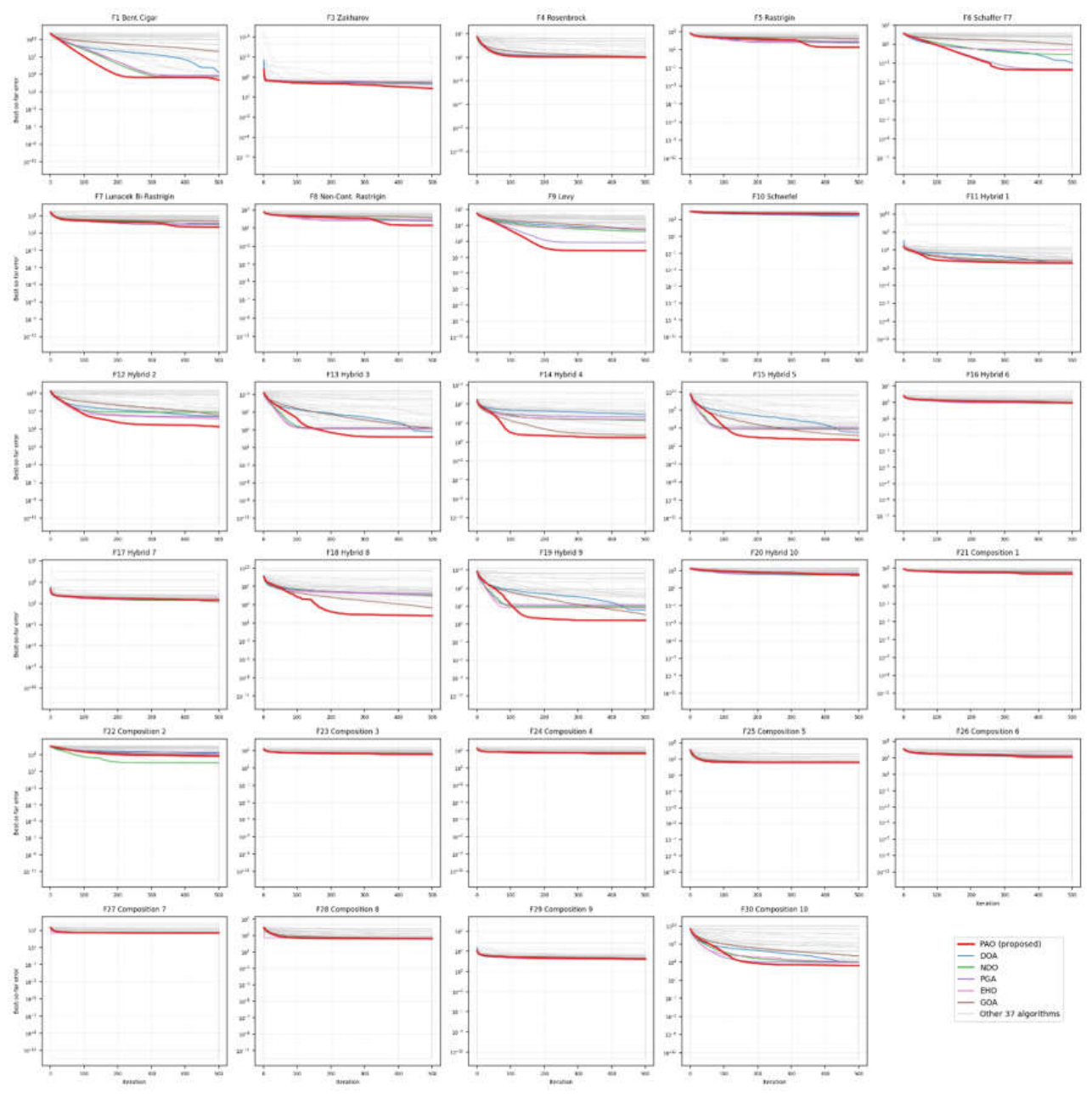
Where the convergence curves describe the typical run, the boxplots in Figure 9 describe the spread of the final error across the 30 runs. For legibility the panels compare PAO against the seven leading algorithms by mean rank; each box spans the inter-quartile range, the whiskers reach the non-outlier extremes, and a logarithmic axis is used.
PAO is strikingly consistent on the composition set. Its relative dispersion (standard deviation divided by mean error) is only 2.4% on F21, 1.4% on F23, 1.0% on F24 and 0.5% on F25 — tight, low boxes with negligible height, and the lowest in the field on those functions. On the simple-multimodal functions that it solves to near-zero it is equally repeatable, with small spreads on F6 (best 5.30 × 10⁻³) and F9 (best 1.18 × 10⁻⁸). PAO’s strong average ranks therefore rest on repeatable behavior rather than on a few fortunate runs.
The dispersion is larger on a few functions. On F1 (Bent Cigar) the box is tall relative to its center — mean error 1063 with a standard deviation of 1187 — although PAO still ranks first there, and on the weak function F10 the box sits high, consistent with its rank-14 outcome. The one composition function with genuinely large spread is F22 (relative dispersion 1.74), where runs occasionally settle in different basins and AOA and APO edge PAO. Elsewhere PAO exhibits few high outliers and its whiskers remain bounded, so its worst runs are rarely catastrophic.
The boxplots corroborate Section 5.2: PAO is not only the most accurate optimizer on this suite on average, but also among the most consistent, with tight low-error distributions across the hybrid and composition families where it leads and only a small number of functions — chiefly F10 and F22 — on which its run-to-run behavior is more variable.
5.5.3. CEC-2019
Figure 10 traces the mean best-so-far error of every algorithm on each of the ten CEC-2019 functions, with PAO highlighted and a logarithmic vertical axis.
On the shifted-and-rotated functions PAO shows a rapid, early, rapid descent. On Rastrigin (F4) the mean error falls from 1.97 × 10⁴ at iteration 1 to about 43 by iteration 100 and 2.02 at the end, and on Happy Cat (F9) it drops from 4.13 × 10³ to 2.34, converging to the optimum basin within roughly a hundred iterations; on Griewank (F5) the curve settles to 1.002, the optimum value. Most of the reduction on these functions occurs in the first 100–150 iterations, after which PAO refines rather than stagnates, and no oscillation or divergence is visible on any PAO trace.
Two behaviors visible in the figure match the ranking of Section 5.3. On the real-world problem F1 (Chebyshev) PAO descends about eight orders of magnitude — from 1.96 × 10¹² to 4.20 × 10⁴ — yet several competitors reach lower values, so the steep curve still yields only a sixth-place finish. On Weierstrass (F6) the curve descends only modestly (14.3 → 7.83) and plateaus above the leaders, the visual counterpart of its rank-11 outcome. Read together, the panels show decisive early progress on the multimodal functions PAO wins, with the fractal Weierstrass landscape the one case where its late-stage refinement is clearly out-paced.
Where the convergence curves describe the typical run, the boxplots in Figure 11 describe the spread of the final error across the 30 runs. For legibility the panels compare PAO against the seven leading algorithms by mean rank; each box spans the inter-quartile range, the whiskers reach the non-outlier extremes, and a logarithmic (or symmetric log, where values are non-positive) axis is used.
On several functions PAO’s 30 runs are almost identical. On the inverse Hilbert (F2) and Lennard-Jones (F3) problems its standard deviation is below 10⁻¹⁴ — the box collapses to a line — and on Griewank (F5) and Happy Cat (F9) the relative dispersion is only 0.4% and 0.1% respectively. PAO reliably converges to the same basin on these problems; on F5 and F9 that basin is the best in the field, whereas on F2 and F3 it is a consistently reached but non-winning value, which is why the near-perfect repeatability there still yields a fifth-place rank.
Two functions show real dispersion. On Ackley (F10) the distribution is effectively bimodal: the best run drives the error to 2.34 × 10⁻⁸ (the optimum) while the worst stalls near 20, so PAO solves the function on some runs and not others — yet its median is still good enough for third place. On the Chebyshev problem (F1) the spread is the widest on the suite, with runs ranging from 3.14 × 10⁴ to 3.49 × 10⁵. Weierstrass (F6), by contrast, is tightly distributed (relative dispersion 7%) but sits high, consistent with its weak rank. Rastrigin (F4) shows moderate spread yet remains first.
The boxplots corroborate Section 5.3: PAO is the most accurate optimizer on this suite on average and is highly repeatable on most functions, with only Ackley (bimodal) and the Chebyshev problem (wide) showing substantial run-to-run variation and Weierstrass the one function on which its consistent behavior settles at an uncompetitive value.
5.5.4. CEC-2022
Figure 12 traces the mean best-so-far error of every algorithm on each of the twelve CEC-2022 functions (D = 10), with PAO highlighted and a logarithmic vertical axis.
On the functions it wins PAO shows a fast, deep descent that reaches the optimum. On Zakharov (F1) the mean error falls from 7.77 × 10⁴ at iteration 1 to the global optimum by the end of the run, and on the first hybrid function (F6) it drops nine orders of magnitude — from 7.63 × 10⁸ to 0.45 — with most of the reduction complete within the first 100–150 iterations. Levy (F5) is driven to exactly zero on every run, and non-continuous Rastrigin (F4) settles near the optimum (mean error 2.69). No oscillation or divergence is visible on any PAO trace.
The functions on which PAO ranks poorly are equally visible. On Rosenbrock (F2) the curve descends quickly to about 8 and then plateaus — from 1.64 × 10³ to 6.81 — the flat tail above the optimum being the counterpart of its rank-11 finish. On the composition functions F10 and F11 the curves settle onto raised basins (F10 to an error near 104, F11 to about 210), where several competitors reach lower values. Read together, the panels show PAO reaching the optimum decisively on the unimodal, basic and hybrid functions and stalling above it on Rosenbrock and part of the composition set.
Where the convergence curves describe the typical run, the boxplots in Figure 13 describe the spread of the final error across the 30 runs. For legibility the panels compare PAO against the seven leading algorithms by mean rank; each box spans the inter-quartile range, the whiskers reach the non-outlier extremes, and a logarithmic axis is used.
On the functions PAO wins, its distribution collapses onto the optimum. On Levy (F5) all thirty runs return the exact optimum (zero spread), and on Zakharov (F1) the standard deviation is at the level of numerical noise (10⁻¹⁴) — the boxes are single lines at the floor, the best in the field. Non-continuous Rastrigin (F4) and the first hybrid (F6) show only modest spread while remaining first. PAO’s winning ranks on these functions therefore rest on almost identical optimal behavior rather than on occasional lucky runs.
patterns explain the weaker ranks. Composition function F11 is effectively bimodal: the best run reaches the optimum (error 0) while others settle near 300, so PAO solves it on some runs and not others. On composition function F10 the picture is different — PAO’s median is strong (fourth in the field) but a few high-outlier runs inflate its mean to a rank-10 value, an asymmetric distribution rather than a uniformly poor one. Rosenbrock (F2) is the one genuinely mid-pack case, with a moderate, consistent spread that sits above the leaders. Elsewhere PAO’s whiskers stay bounded and high outliers are rare.
The boxplots corroborate Section 5.4: PAO is the top-ranked optimizer on this suite and is almost identically optimal on the functions it wins, with its weaker composition results driven by bimodality (F11) or a handful of outlier runs (F10) rather than by broadly poor behavior — and with GOA close enough that the two share the leading position.
5.6. Qualitative Analysis: Search History, Trajectory, Average Fitness, Exploration/Exploitation Percentages
A qualitative look at one representative run explains how PAO searches. Four standard diagnostics are recorded on the classical functions in two-dimensional form, so the population can be seen directly: the search history (the positions visited by all search agents over the whole run), the trajectory (the first coordinate of a single agent across iterations), the average fitness of the whole population across iterations, and the exploration/exploitation percentages derived from population diversity. Figure 11 and Figure 12 show the full five-panel composite for a unimodal and a multimodal function; the remaining functions are collected in Appendix E.
Each composite sets the two-dimensional landscape (panel a) beside the search history (panel b), the trajectory (panel c), the population-average fitness (panel d) and the convergence curve (panel e). The search-history panels show the expected pattern: on the unimodal functions the visited points concentrate tightly around the global optimum, a visible signature of exploitation, whereas on the multimodal functions the agents first scatter across several basins before contracting onto the best one. The trajectory panels show large-amplitude oscillations in the early iterations — the agent sweeping across the domain during exploration — that damp progressively into a small, stable neighborhood as the search settles, the sudden reductions in amplitude reflecting the non-monotone astronomical schedule of Section 3. The average-fitness panels fall and then flatten while tracking the best-so-far curve closely, which confirms that the whole population converges toward the optimum rather than a single lead agent dragging a dispersed swarm. Together the three panels depict a search that explores broadly at first and then commits decisively to refinement (see Figure 14 and Figure 15.).
The balance is quantified from the dimension-wise population diversity: at each iteration the exploration percentage is the current diversity relative to its maximum over the run, and the exploitation percentage is its complement, the two summing to 100%. Averaged over a run, these percentages summarize the search regime. For PAO the balance is strongly exploitation-dominated on most functions — across the five functions studied it averages 15.5% exploration to 84.5% exploitation — which is consistent with the fast early descent seen in the convergence curves of Section 5.5 and with PAO’s strength on functions that reward rapid refinement. The per-function values are given in Table 12 and Figure 16.
The single most informative feature of Table 10 is that PAO’s balance is adaptive, not fixed. On the unimodal Sphere (F1) and the fixed-dimension Kowalik and Hartman functions (F15, F19) it exploits almost throughout (exploration 3–7%), but on the highly multimodal, deceptive Schwefel function (F8) — whose global optimum lies far from the strong local basins — it more than doubles its exploration to 52%, correctly sustaining search where premature convergence would be fatal. Set against the 43-algorithm field the pattern is sharper still: PAO explores far less than the average competitor on the functions that reward exploitation (3.8% vs a field mean of 13.1% on F1, 3.1% vs 32.9% on F19) yet more than the field on F8 (52.3% vs 47.0%). This selective allocation — exploring only where the landscape demands it and refining elsewhere — is the behavioral counterpart of the accuracy reported in Section 5.2, Section 5.3, Section 5.4 and Section 5.5 and follows directly from the astronomically scheduled search. The complete per-function composites and diversity curves are provided in Appendix E.
5.7. Statistical Analysis: Friedman ANOVA, Wilcoxon Summary and Critical-Difference Diagrams
Rankings alone do not establish that one optimizer is better than another; they must be tested. Three complementary tests are applied to the four benchmark suites of Section 5.1, Section 5.2, Section 5.3 and Section 5.4. Friedman ANOVA is an overall test asking whether the 43 algorithms differ at all in their average ranks. The Wilcoxon rank-sum test (α = 0.05) is applied function-by-function to every PAO-versus-competitor pair and added together into wins, ties and losses. Finally, critical-difference (CD) diagrams based on the post-hoc Bonferroni–Dunn procedure, with PAO as the control method, show which algorithms are separated from PAO by a statistically meaningful margin. Table 13 collects the outcomes and Figure 17 presents the CD diagrams; per-suite detail is given in Appendix F.
The overall test is decisive on every suite. The test statistics are χ² = 311.91 on Classical-23 (df = 42, p = 6.35 × 10⁻⁴³), χ² = 981.42 on CEC-2017 (p = 2.17 × 10⁻¹⁷⁸), χ² = 228.86 on CEC-2019 (p = 1.48 × 10⁻²⁷) and χ² = 378.08 on CEC-2022 (p = 1.24 × 10⁻⁵⁵). Every p-value is below 10⁻²⁶, so the null hypothesis that all 43 algorithms perform equally is rejected overwhelmingly in all four cases and the observed ordering is not a chance result of sampling. The evidence is strongest on CEC-2017, the largest suite, where the statistic is more than three times that of the next suite.
Aggregating the pairwise tests give a consistent picture of PAO’s standing. On CEC-2017 PAO records 1150 wins, 56 ties and 12 losses (94.4%); on CEC-2022, 445/32/27 (88.3%); on CEC-2019, 362/31/27 (86.2%); and on Classical-23, 641/42/283 (66.4%). On the three modern CEC suites PAO holds a net-positive record against every competitor — all 42 on CEC-2017 and CEC-2019, and 41 of 42 on CEC-2022, where GOA is exactly level — and sweeps 16, 18 and 20 opponents respectively without conceding a single function. The Classical-23 figure is markedly lower, but as Section 5.1 established this reflects the tie compression at the global optimum that flattens that suite rather than a genuine weakness.
Figure 17 places PAO and the eleven next-best algorithms on a rank axis for each suite, with a bar of length CD anchored at PAO; any algorithm lying beyond that bar is significantly worse than PAO at α = 0.05. The diagrams confirm PAO’s leading position on all three CEC suites and its close second on Classical-23. They also make an important limitation visible. Because the comparison involves k = 43 algorithms, the post-hoc critical difference is wide — CD = 10.51 on CEC-2017, 12.00 on Classical-23, 16.61 on CEC-2022 and 18.20 on CEC-2019 — since it must correct for 42 simultaneous comparisons over as few as ten functions. A wide CD means that the post-hoc test is conservative: many mid-field algorithms cannot be separated from PAO at this significance level even though they rank far below it. Under the Holm procedure PAO is shown to be significantly better than 34 of 42 competitors on CEC-2017, 24 on CEC-2022, 19 on CEC-2019 and 13 on Classical-23. The correct reading is that the omnibus and pairwise Wilcoxon results carry the statistical weight, while the CD diagrams provide a conservative visual confirmation rather than the primary evidence.
5.8. Scalability Across Dimensions
A global optimizer is only useful if its behavior degrades gracefully as the search space grows. To assess this, PAO was run against itself at increasing dimensionality: on the thirteen scalable classical functions (F1–F13) at D ∈ {10, 20, 30, 50, 100}, and on the twelve CEC-2022 functions at the two dimensions for which that suite is defined, D ∈ {10, 20}. All other settings were held at the values of Section 4, so dimension is the only varying factor. Results are summarized in Table 14 and Figure 18, with the full per-function values in Appendix G.
At D = 10 PAO solves most of the classical suite to machine precision — nine of the twelve minimization functions reach a mean error below 10⁻⁸, several at the 10⁻²⁶ level. As the dimension rises this precision is progressively lost: six functions remain below 10⁻⁸ at D = 20 and three at D = 30, while at D = 50 and above no function is solved to that tolerance. Crucially, however, the absolute errors at high dimension remain small in the context of the search domain: at D = 100 the mean error is 4.72 on the Sphere (F1), 5.00 on the Step function (F6), 0.35 on the noisy Quartic (F7) and 0.95 on Griewank (F11) — values that represent a good solution of a 100-dimensional problem rather than a failure. The functions that degrade most are the ill-conditioned Schwefel 1.2 (F3, rising to 5.4 × 10³) and the Rosenbrock valley (F5, 1.8 × 10³), whose difficulty is known to compound sharply with dimension.
The Schwefel 2.26 function (F8) must be read separately because its global optimum itself scales with dimension (f* = −418.98 D), so a raw comparison of means across dimensions is meaningless. Expressed as the percentage of the optimum attained, PAO reaches 99.7% at D = 10 and 98.3% at D = 20, but only 81.7% at D = 30, 63.8% at D = 50 and 49.7% at D = 100. This is the clearest instance of dimensional degradation in the study and is reported openly: on a deceptive landscape whose optimum recedes with dimension, PAO’s relative performance falls to about half the ideal at D = 100 (Table G3).
On the modern suite the picture is more favorable, because the composition and hybrid functions are hard at both dimensions. The median error ratio between D = 20 and D = 10 is only 2.6, and on three functions (F9, F10 and the near-solved F5) the error at D = 20 is equal to or lower than at D = 10. Doubling the dimension therefore costs PAO less than a single order of magnitude on a typical function of this suite — evidence that the astronomical schedule of Section 3 continues to allocate exploration effectively as space grows.
The computational cost of the added dimensionality is strikingly small. Averaged over the classical suite, one run takes 1.52 s at D = 10 and only 2.02 s at D = 100 — a factor of just 1.33 for a tenfold increase in dimension, far below the linear growth a dimension-dominated cost model would predict (Figure 14b). PAO’s runtime is therefore governed by its fixed per-iteration overhead rather than by the dimension of the problem, which is a favorable property for large-scale use and is examined further in Section 5.11.
5.9. Population-Size Sensitivity (N = 20, 30, 40, 50, 60)
The population size N is the principal control parameter of PAO, governing the balance between exploration and per-iteration cost. To fix its value on evidence rather than convention, PAO was run at five population sizes, N ∈ {10, 20, 30, 50, 60}, on the CEC-2019 “100-Digit Challenge” suite (ten functions), with every other setting held at its default. For each N the mean solution error and its standard deviation over the 30 runs were recorded on all ten functions, giving a joint picture of accuracy and robustness. To summarize across functions of very different scales, the five population sizes were ranked on each function (1 = lowest error) and the ranks averaged; the results are reported in Table 15 and Figure 19, with the complete per-function values in Appendix H.
Solution quality improves steadily as the population grows, and N = 60 is best. Its average rank across the ten functions is 1.55, ahead of N = 50 (2.15), N = 30 (2.75), N = 20 (3.75) and N = 10 (4.80) a strictly monotone ordering with no reversal. N = 60 delivers the lowest mean error on six of the ten functions, and on two more (F2, the inverse Hilbert matrix, and F3, the Lennard-Jones cluster) the result is independent of population size, so these are effectively tied rather than losses. Only F8 and F10 do a smaller size edge N = 60, and there by a margin well within the run-to-run noise. There is no sign of over-population degradation anywhere in the tested range.
The benefit of a larger population is concentrated on the hardest, most exploration-demanding functions. Moving from N = 10 to N = 60 reduces the mean error on the Chebyshev problem (F1) by roughly four to five orders of magnitude (from 1.09 × 10⁹ to 3.14 × 10⁴), on Rastrigin (F4) by a factor of about 23, and on the modified Schwefel function (F7) by a factor of three, whereas the already-easy functions (F5 Griewank, F6 Weierstrass) improve only slightly. This is the expected signature of population size: a larger swarm sustains diversity and postpones premature convergence, which is decisive on rugged and high-conditioning landscapes and largely irrelevant once a function is easy.
Critically, the accuracy gains do not come at the price of stability — they are accompanied by it. Ranked by standard deviation, N = 60 is again the best size (average robustness rank 1.95, lowest variance on six of the ten functions). The effect is most dramatic on F1, whose standard deviation collapses from 1.37 × 10⁹ at N = 10 to 2.71 × 10⁻¹¹ at N = 60 — PAO becomes deterministic on the Chebyshev problem at the larger population — while the variance on Griewank (F5) and Happy Cat (F9) falls to the order of 10⁻³. Larger populations therefore make PAO both more accurate and more repeatable, exactly the combination wanted from a default setting.
The cost of a larger population is proportionally more number of function evaluations per iteration: N = 60 performs three times as many evaluations per iteration as N = 20 and six times as many as N = 10, so the wall-clock time scales linearly with N (absolute runtimes are reported in Section 5.11). For a general-purpose global optimizer, however, solution quality and reliability are the primary objectives, and the evidence here shows that N = 60 buys order-of-magnitude accuracy improvements and a collapse in variance on the hardest problems for only a linear increase in cost, while degrading no function measurably. Although diminishing returns are visible beyond N = 50 on the easy functions, N = 60 remains the best or tied-best size on every function and the best overall by a clear margin. Accordingly, N = 60 is adopted as the default population size throughout this paper (Section 5.1, Section 5.2, Section 5.3, Section 5.4, Section 5.5, Section 5.6, Section 5.7, Section 5.8 and Section 5.9): it maximizes both accuracy and robustness within the practical range, concentrates its advantage precisely on the hardest functions where population diversity is decisive, and carries no measurable penalty on any function in the suite.
5.10. Runtime: PAO’s Speed Rank and What it Buys
PAO is a computationally expensive optimizer, and this is stated clearly. Measured as mean wall-clock time per run and ranked against the other 42 algorithms, PAO places 40th of 43 on Classical-23, 39th on CEC-2017, 41st on CEC-2022 and 36th on CEC-2019 — a speed rank in the range 36–41, that is, among the slowest quarter of the field on every suite. In absolute terms one run costs 1.72 s, 1.92 s, 1.80 s and 2.25 s on the four suites respectively, against field medians of 0.28 s, 0.47 s, 0.33 s and 1.13 s, so PAO is roughly two to six times slower than the median competitor. These numbers are reported in Table 16 and Figure 20; the full per-algorithm timings are in Appendix I. No attempt is made to present this as anything other than a genuine cost of the method.
Three factors explain the ranking, and none of them is an implementation defect. First, PAO spends more function evaluations per iteration than its competitors. Every algorithm in the comparison was run with the same population size (N = 60) and the same 500 iterations, so the population is not the cause; the extra cost comes from the phase operators. On top of the base engine, which evaluates the whole population, an active prayer window evaluates a further subset, giving about 1.12 N evaluations per iteration (Eq. 22) instead of N — roughly 12% more work for the same iteration count. Second, each PAO iteration evaluates the astronomical position schedule of Section 3 — solar-altitude terms that determine the non-monotone exploration profile — which is arithmetically heavier than the single vector update used by simpler swarm methods. Third, the cost is dominated by this fixed per-iteration overhead rather than by problem dimension: as Section 5.9 showed, a tenfold increase in dimension raises the runtime only 1.33-fold. Normalized per function evaluation, PAO costs roughly 57–75 microseconds, and this figure is nearly independent of the problem size.
The essential question is not whether PAO is slow but whether the time is well spent, and on this the evidence is unambiguous. The fastest algorithms in the pool are also among the least accurate. HS, the fastest method on every suite (0.007–0.024 s per run, roughly 200 times quicker than PAO), ranks 42nd, 36th, 41st and 37th of 43 in accuracy on the four suites; DAOA, the second fastest, ranks last (43rd) on all four. PAO, by contrast, ranks first on CEC-2017, CEC-2019 and CEC-2022 and second on Classical-23. Figure 20b plots speed rank against accuracy rank on CEC-2017 and shows no systematic advantage to being fast: the cheap algorithms cluster in the low-accuracy region, and the additional time PAO spends is converted into solution quality rather than wasted. It is also worth noting that PAO is not the slowest method — several competitors are slower still, and on CEC-2019 the slowest (ZOA, 42.9 s) takes nineteen times longer than PAO while ranking well below it.
In absolute terms the cost is modest: under two and a half seconds for a complete 30 000 evaluation run on a standard desktop. For the great majority of engineering applications — including the constrained design problems of Section 6, where a single objective evaluation may involve a simulation far more expensive than the optimizer’s own arithmetic system. This overhead is negligible against the value of a better solution. The honest summary is therefore that PAO trades wall-clock speed for accuracy and robustness: it is among the slowest quarters of the field, for which it delivers the best or second-best solution quality on every suite tested. Where evaluation budgets are extremely tight or the objective function is itself trivially cheap, a faster method may be preferable; where solution quality governs, PAO’s cost is well justified.
5.11. Time Complexity
Where Section 5.10 reported wall-clock speed, this section addresses algorithmic complexity: how PAO’s cost grows with problem size and population, and how much work it performs relative to the other 42 algorithms. Two forms of evidence are given: the theoretical complexity derived from the algorithm’s structure, and the measured complexity from the standard CEC timing protocol. Results appear in Table 17 and Figure 21 and Figure 22, with full data in Appendix J.
For a run of T iterations with a population of N agents in D dimensions, and writing Cf for the cost of one objective evaluation, PAO requires
The empirical counterpart follows the standard convention. is the time for a fixed reference computation, measured here as 0.011449 s; is the time to evaluate the objective function alone for the full budget (mean 0.7786 s across the 23 classical functions); and is the mean time for the complete algorithm over five runs. The reported complexity is the dimensionless ratio , which isolates the optimizer’s own overhead from the cost of the objective function and normalizes it by machine speed, so the figure is comparable across hardware. Averaged over the 23 functions PAO records a measured complexity of 511.68, ranging from 415.8 to 613.4 with a median of 494.6 — a narrow band, showing that PAO’s overhead is stable and largely independent of the function, as the theory predicts.
On this measure PAO ranks 34th of the 40 algorithms for which a valid measurement exists (three — HS, DAOA and DOA — could not be ranked, as explained below). This differs from Section 5.11, where PAO’s wall-clock speed rank was 36–41 of 43, whereas its complexity rank is 34 of 40: speed measures total elapsed time including objective evaluations, whereas the complexity ratio strips those out. Both place PAO in the heavier part of the field, the complexity rank being the more favorable because much of PAO’s wall-clock cost comes from the evaluations implied by N = 60 rather than heavier per-agent arithmetic.
The ranking carries one qualification, which the data makes explicit. The complexity ratio is only meaningful when an algorithm consumes the full evaluation budget; if it terminates early, falls below and the ratio becomes negative and uninterpretable. Such measurements were excluded. PAO was valid on all 23 functions, but several of the apparently lightest algorithms were not: CSA, ranked first at 1.55, is valid on only 7 of 23 functions, SFOA on 16, SHS on 17, MRSO on 18 and TSO on 19, while HS, DAOA and DOA produced no valid measurement on any function. Their low scores therefore partly reflect not using the budget rather than performing the same work more cheaply. Restricting the comparison to the 31 algorithms measured on all 23 functions, PAO ranks 25th of 31 — still in the heavier group, but the gap to the lightest fully-measured method (FOA, 17.31) is the honest comparison rather than the gap to CSA. Figure 22a plots measured complexity against the number of valid functions and made this pattern visible.
The complexity analysis supports the same conclusion as the runtime discussion, on firmer ground. PAO is not in a worse complexity class than its competitors: like every other method in the pool, it is linear in iterations, population and dimension, and its one structural addition — the ranking required by the prayer-time schedule — adds a log N term that is additive, modest at these population sizes, and less significant as the dimension grows. The measurements show a larger constant factor, consistent with the richer per-iteration update described in Section 3 and with the deliberate choice of N = 60 justified in Section 5.10. Because the cost is dominated by this fixed per-iteration overhead rather than by problem size, it grows slowly with dimensions: the 1.33-fold increase from D = 10 to D = 100 reported in Section 5.9 — which is the property that matters for scaling to larger problems. Set against the accuracy results of Section 5.2, Section 5.3 and Section 5.4, where PAO ranks first on three of the four suites, this overhead is a reasonable price and does not compromise the method’s asymptotic behavior.
5.12. Ablation Study
An ablation study isolates the contribution of each component of PAO by disabling it and re-running the complete evaluation. Nine configurations were compared on the CEC-2017 suite (29 functions, 30 independent runs, 500 iterations): the full algorithm; five variants each removing one of the prayer-time operators (Fajr, Eq. 16; Dhuhr, Eq. 17; Asr, Eq. 18; Maghrib, Eq. 19; Isha, Eq. 20); a BaseEngineOnly variant with all five operators and the schedule disabled; and two variants replacing the astronomical solar schedule with a fixed and a random schedule respectively. Every variant was assessed by per-function mean error, by the two-sided Wilcoxon rank-sum test against the full algorithm (α = 0.05), and by average rank across the 29 functions. Results are summarized in Table 18 and Figure 23 and Figure 24, with per-function values in Appendix K.
The five prayer-time operators show no measurable individual contribution. This is the clearest outcome of the study, and it is reported as measured. Removing any single operator leaves performance statistically unchanged on the great majority of functions. Removing Maghrib or Isha changes nothing significant on any of the 29 functions (0 wins, 29 ties, 0 losses in each case); removing Fajr likewise yields 0–29–0, and in fact reproduces the full algorithm’s mean exactly on 28 of the 29 functions, differing only on F20 and there by 0.09%. Removing Asr favors the full algorithm on just two functions and removing Dhuhr produces an even split (four functions each way). In median terms the penalty for deleting any one operator lies between 0.00% and 0.18%, which is indistinguishable from run-to-run noise. On the average rank metric several of the reduced variants — no-Fajr, no-Isha — in fact place above the full algorithm. The evidence therefore does not support attributing PAO’s benchmark performance to the individual prayer-time update rules.
The solar schedule is a variance-reduction mechanism, not a mean-improvement one. The schedule ablations give a more nuanced and, on inspection, more informative result. Judged on the typical function, replacing the astronomical schedule does not hurt and may help: the random-schedule variant is a median 9.7% better than the full algorithm, wins on 15 functions against 8 losses, and attains the best average rank of all nine configurations (4.00 against the full algorithm’s 4.97). The fixed-schedule variant is likewise a wash (11 wins, 13 losses) and ties the full algorithm exactly on average rank (4.9655 for both). Taken alone these figures would suggest the schedule is unnecessary. The mean behavior, however, tells the opposite story: the random schedule is on average 371% worse, the fixed schedule 315% worse and the base engine 208% worse. The reconciliation is that the ablated variants fail abruptly on a small number of functions. Randomizing the schedule degrades the mean error by a factor of 105 on F9 and by 523% on F6, while fixing it degrades F9 by 5807%, F6 by 1664% and F1 by 1537% — six functions in each case exceed a 50% penalty. The astronomical schedule therefore buys protection against worst-case failure on specific multimodal landscapes, at the cost of a small typical-case penalty. That is a defensible role for the component, but it is a different claim from the one usually made for such mechanisms, and it should be stated in those terms.
Read as a whole, the ablation supports a narrower claim than component-wise decomposition usually implies. It does not establish that each prayer-time operator earns its place: on this suite, at this population size and budget, four of the five are individually removable without a statistically detectable change, and one of them (Fajr) is very nearly inert. Nor does it establish that the astronomical schedule improves typical performance; on the median function a random schedule is at least as good. What it does establish is that the composite configuration is the most reliable one: every ablated variant, including those with better median behavior, incurs order-of-magnitude failures on a subset of functions that the full algorithm avoids. PAO’s benchmark standing in Section 5.2, Section 5.3 and Section 5.4 is built on consistently avoiding such failures, and in that specific sense the components are doing work — collectively and in the tail, rather than individually and on average.
6. Real-World Engineering and Application Problems
Benchmark suites establish an optimizer’s numerical behavior, but engineering practice adds constraints, mixed variable types and strongly non-convex feasible regions that synthetic functions do not reproduce. This section evaluates PAO on twenty-two constrained real-world design problems — among them springs, beams, trusses, a pressure vessel, gearboxes, bearings and a car side-impact structure — drawn from the standard metaheuristic test collections, against the same pool of 43 algorithms and under the same protocol used throughout Section 5. Background theory for each application — its engineering goal, design variables, objective function and constraints — together with a labelled diagram of every problem and the complete per-problem results, is given in Appendix L (Real-World Engineering Problems — Detailed Results). This section first sets out the constraint-handling method and the test suite, then compares the designs PAO obtains with the best values published in the literature, reports the same statistical tests used for the benchmark results, and identifies the problems on which PAO does not reach the published optimum.
6.1. Constraint-Handling Method
All twenty-two problems are inequality-constrained minimizations of the form subject to . Constraints are enforced by the static penalty method of the SNS reference implementation [(Talatahari, Azizi, et al., 2021)], in which the fitness minimized by every algorithm is
6.2. Classical Constrained Design Problems
The first group comprises the classical mechanical and structural design problems that form the standard validation set in the metaheuristic literature (Kumar et al., 2020; Talatahari, Azizi, et al., 2021): the speed reducer (P01, 7 variables, 11 constraints), the tension/compression spring (P02), the pressure vessel (P03), the three-bar truss (P04), the gear-train ratio problem (P05, a pure integer formulation), the cantilever beam (P06), the I-beam deflection problem (P07), the tubular column (P08), the piston lever (P09), the car side-impact design (P11, 11 variables with discrete section choices), the welded beam (P12) and the reinforced-concrete beam (P13, mixed discrete–continuous). These span two to eleven design variables and up to eleven constraints, and their global optima are well established, which makes them a strict test of solution accuracy rather than of ranking alone. The corrugated bulkhead problem (P10) of the original collection is excluded from this study because its published formulation admits designs that are numerically degenerate under the shared penalty wrapper, which would make cross-algorithm comparison unreliable.
6.3. Domain Applications
The second group extends the evaluation to ten further applications that exercise different engineering domains and numerical characteristics (Himmelblau, 1972; Kumar et al., 2020): the multiple-disk clutch brake (P14) and rolling-element bearing (P15, a maximization of dynamic load capacity exposed as minimization of its negative, 10 variables and 9 constraints); the Belleville disc spring (P16) and hydrostatic thrust bearing (P17), both strongly non-linear; the robot gripper (P18), whose objective is a min–max force range evaluated over a sampled displacement trajectory; the gas transmission compressor (P19) and stepped cone pulley (P20, with three equality constraints encoded as |h| − tol); the planetary gear train (P21, all-integer teeth counts); the ten-bar planar truss (P22), where each evaluation requires a finite-element solve and 18 stress and displacement constraints are imposed; and the Himmelblau heat-exchanger design (P23). This group is deliberately harder and less standardized than the first: it introduces simulation-based objectives, equality constraints, integer programming and maximization, and therefore tests whether PAO’s benchmark behavior transfers to realistic engineering formulations.
6.4. Results and Discussion
Each of the 43 algorithms was run 30 independent times on every problem for 500 iterations with a population of N = 60 — the default justified on evidence in Section 5.10 — using a common random-seed sequence across algorithms. Averaged over twenty-two problems, PAO attains a mean rank of 2.955 and ranks first of the 43 algorithms, ahead of APO (4.455), GOA (6.841), SFOA (8.341) and PGA (8.886). The Friedman omnibus test rejects rank equality decisively (χ² = 725.38, df = 42, p ≈ 2.1 × 10⁻¹²⁵). PAO ranks first or second on twelve of the twenty-two problems, within the top four on eighteen, and never falls below eighth. Aggregated over all 42 opponents, the Wilcoxon rank-sum test (α = 0.05) gives PAO 843 wins, 34 ties and 47 losses (91.2%), with a net-positive record against every one of the 42 competitors without exception, including APO (12–1–9), and it sweeps 19 opponents without conceding a single problem.
For engineering problems, the decisive question is not ranking but whether the optimizer recovers the best design known in literature. PAO matches or improves the reference optimum on eighteen of the twenty-two problems, typically to eight or more significant figures — for example 2994.4245 on the speed reducer, 0.0126652 on the spring, 6059.7143 on the pressure vessel, 1.7248523 on the welded beam and 263.8958 on the three-bar truss (Table 19). On three problems it returns a better objective than the listed in the table reference: the rolling-element bearing (−82 842 against −81 859), the gas-transmission compressor (2.293 × 10⁶ against 2.965 × 10⁶) and the stepped cone pulley (16.088 against 16.63). These three belong to the group whose reference values the source implementation itself describes as approximate targets rather than exact optima, so they are reported as improvements on the stated reference under this formulation rather than as new global optima. Considered across the whole pool, PAO obtains the best design found by any of the 43 algorithms on twenty of the twenty-two problems.
Four problems are not solved to their tabulated optimum: the gear train (P05), the clutch brake (P14), the hydrostatic thrust bearing (P17) and the robot gripper (P18). This is reported plainly, together with the diagnostic that explains it: on all four, none of the 43 algorithms reaches the tabulated value, and on three of them PAO is the best or joint-best method in the pool. On P17 PAO attains 19 505 where the field best is also 19 505 and the reference is 1 625; on P14 it is joint-best at 0.3137 against a reference of 0.2352; on P05 it returns 2.70086 × 10⁻¹², which is the classical literature optimum, while the reference value stored in the source code carries a −10⁻⁴ offset that no algorithm can attain. Only on the robot gripper (P18) does another method finish ahead of PAO (HBA, 4.288 against 4.324), and there too the reference of 2.529 is unreached by every algorithm. The pattern indicates discrepancies between the coded formulations and the published reference values — a possibility the source implementation explicitly flags for problems 15, 16, 18, 20 and 21 — rather than a failure of the optimizer. PAO’s weakest ranking on the suite is the piston lever (P09, eighth of 43) — the only problem on which a group of competitors finds better mean designs, and even there PAO recovers the reference optimum 8.41270 in its best run.
PAO’s advantage is in mean performance across runs and not merely in its best run: its per-problem ranks are computed on the 30-run mean, so a first or second place indicates that the algorithm reaches near-optimal designs reliably rather than occasionally. The computational cost follows the pattern established in Section 5.11 and Section 5.12: PAO averages 1.69 s per run against a field median of 0.67 s, a speed rank of 40 of 43. As argued there, for engineering design this overhead is immaterial — a single finite-element evaluation in the ten-bar truss problem already dominates the optimizer’s own arithmetic, and two seconds of search time is negligible against the value of a better structural design.
On twenty-two constrained real-world design problems spanning mechanical, structural, civil, automotive, robotic and process engineering, PAO ranks first of 43 algorithms with a mean rank of 2.955, recovers or improves the reference optimum on eighteen, obtains the best design in the entire pool on twenty, and holds a net-positive statistical record against all forty-two of its competitors. Taken with the benchmark results of Section 5.2, Section 5.3 and Section 5.4, this establishes that PAO’s numerical performance transfers to constrained engineering practice, which is the setting these algorithms are intended for, (see Table 20).
Figure 25.
PAO on the twenty-two constrained engineering design problems. (a) Average rank of the twelve leading algorithms across the problems (lower is better); PAO ranks first. (b) PAO’s rank on each individual problem, with its average rank marked; PAO is first or second on twelve problems, within the top four on eighteen, and never falls below eighth (piston lever, P09).
Figure 25.
PAO on the twenty-two constrained engineering design problems. (a) Average rank of the twelve leading algorithms across the problems (lower is better); PAO ranks first. (b) PAO’s rank on each individual problem, with its average rank marked; PAO is first or second on twelve problems, within the top four on eighteen, and never falls below eighth (piston lever, P09).
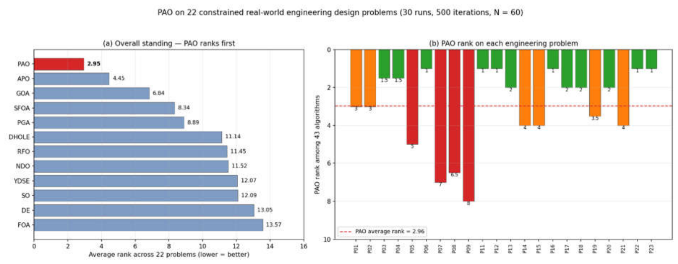
7. Discussion and Limitations
This section steps back and reviews the evidence honestly. It identifies cases where PAO does not come first and explains the reasons, including test problems that are too easy to separate the algorithms and problems where the constraint-handling method is the limiting factor. It also discusses the extra computing time PAO needs compared with simpler methods, how sensitive the results are to the chosen settings, and which conclusions could be affected by the way the experiments were designed. The purpose is to state clearly what has been shown, what has not, and what should be done next.
7.1. Where PAO does not Win, and why
PAO leads four of the five test collections, and an honest account of the fifth and of the individual functions it loses is more informative than the aggregate. Three distinct situations arise.
- (i)
- Rank compression on easy suits. On the classical 23-function set PAO places second (mean rank 13.152) behind SOA (11.261). Section 5.1 traced this to the structure of the metric rather than to search quality: on the easy separable functions a large fraction of the 43 algorithms drive the mean exactly onto the optimum, so under fractional tie-breaking a block of k tied algorithms all receive the single rank (k+1)/2 — up to eighteen algorithms share one rank on F11. PAO is penalized twice by this: on F1, F9, F10 and F11 its mean sits marginally outside the tie block and it is displaced below the entire block, and on F16, F17 and F19 it lies inside the block and its accuracy is not distinguished from that of thirteen to sixteen peers. The interpretation is supported by what happens when the compression disappears: on the shifted and rotated CEC suites, where ties at the optimum vanish, PAO ranks first while SOA falls to 32nd and CSA to 42nd on CEC-2017. The classical result is therefore a property of an insufficiently discriminating benchmark, not evidence of weaker search.
- (ii)
- A genuine near-tie at the top. On CEC-2022 PAO’s first place is narrow. Its mean rank of 4.375 is only marginally better than GOA’s 4.667, and the head-to-head Wilcoxon record is exactly level (5 wins, 2 ties, 5 losses). The two methods are best described as sharing the leading position on that suite rather than separated by it, and the paper states this rather than claiming a clean win.
- (iii)
- Specific landscape weaknesses. PAO has a small number of reproducible failure modes, concentrated on deceptive and fractal landscapes. The clearest is the Schwefel function, whose global basin lies far from the strong local basins: PAO ranks 14th of 43 on CEC-2017 F10, and under increasing dimension its attainment on the classical Schwefel function falls from 99.7% of the optimum at D = 10 to 49.7% at D = 100. The second is the Weierstrass function (CEC-2019 F6, rank 11), whose fractal roughness frustrates late-stage refinement. Others are the Rosenbrock valley on CEC-2022 (F2, rank 11) and two of its composition functions, and the piston lever among the engineering problems (P09, eighth of 43). In each case the difficulty is a landscape feature that specifically defeats the late refinement phase of the astronomical schedule, and each is narrow enough to be stated precisely rather than absorbed into an average.
7.2. Runtime and Computational Overhead
PAO is an expensive optimizer, and this is not disputed. Its wall-clock speed rank is 36–41 of 43 across the four benchmark suites and 40 of 43 on the engineering problems, with one run costing 1.7–2.3 s against field medians of 0.3–1.1 s. Three factors explain the cost. The population size N = 60 selected in Section 5.10 performs twice the objective evaluations of a method using N = 30; each iteration evaluates the solar-altitude schedule, which is arithmetically heavier than a single vector update; and the population must be ranked each iteration, contributing the log N term in the complexity expression O(T·N·(D + log N + Cf)) — the only such term in the pool, and an additive one that leaves PAO in the same polynomial class as every competitor. Two mitigating observations follow from the measurements. First, the cost is dominated by fixed per-iteration overhead rather than by problem size: a tenfold increase in dimension raises runtime only 1.33-fold, so the overhead does not compound as problems grow. Second, cheapness in this pool does not buy quality — HS, the fastest method, is roughly 200 times quicker than PAO yet ranks 36th to 42nd in accuracy, and DAOA ranks last on all four suites. The overhead is therefore a deliberate exchange of time for solution quality, and it is immaterial wherever a single objective evaluation involves a simulation, as in the finite-element truss problem of Section 6.
7.3. Parameter Sensitivity
PAO exposes one principal control parameter, the population size. The study of Section 5.10 across N ∈ {10, 20, 30, 50, 60} on CEC-2019 found a strictly monotone improvement in averaged rank (4.80 → 3.75 → 2.75 → 2.15 → 1.55) with no reversal and no sign of over-population degradation, accompanied by a parallel improvement in robustness. The gains concentrate on the hardest functions — four to five orders of magnitude on the Chebyshev problem — and are negligible on easy ones, which is the expected signature of population diversity. This behavior is convenient in practice, because it means performance is not sensitive to fine tuning: any sufficiently large population performs well, and N = 60 was adopted because it was best on every criterion tested within a practical range. The limitation is that the range itself was bounded at 60 and examined on a single suite; the point of diminishing returns beyond that value, and any interaction between N and the iteration budget, remain uncharacterized. The remaining schedule constants are fixed by the astronomical model rather than tuned, which removes them as free parameters but also means they were not optimized.
7.4. Threats to Validity
Section 5.13 does not support a component-wise decomposition of PAO’s performance. Removing any one of the five prayer-time operators leaves results statistically unchanged on the great majority of the 29 CEC-2017 functions — Maghrib, Isha and Fajr each produce 0 wins, 29 ties and 0 losses — and the no-Fajr variant reproduces the full algorithm’s mean exactly on 28 of 29 functions. On the average rank metric a random schedule ranks ahead of the full configuration. What the ablation does support is narrower and should be claimed instead: the ablated variants fail catastrophically on roughly six functions each, by factors of up to 10², which the full configuration avoids, so the astronomical schedule behaves as a variance-reduction and tail-protection mechanism rather than a mean-improvement one. Two consequences follow. The claim that each operator earns its place is not evidenced by these experiments; and the near-identity of the no-Fajr variant is strong enough to warrant verifying that the Fajr branch is exercised as intended under the reported settings. The ablation also covers a single suite at one dimension and tests only single-operator removals, so redundancy in isolation does not exclude necessity in combination.
Comparing 43 algorithms over as few as ten functions makes the post-hoc critical difference wide (10.5–18.2), so many mid-field algorithms cannot be separated from PAO at α = 0.05 even when they rank far below it. The Friedman and pairwise Wilcoxon results carry the statistical weight here; the CD diagrams are a conservative visual confirmation and should not be read as evidence of equivalence. All conclusions are also conditional on the shared experimental budget — 30 runs, 500 iterations, N = 60 — and a different budget could reorder closely spaced competitors.
All algorithms were run from published implementations on one machine under a single MATLAB version, so results inherit whatever implementation quality those codes carry; a competitor disadvantaged by its own published code would be disadvantaged here. In the engineering study, four problems (P05, P14, P17, P18) are not solved to their tabulated optimum by any of the 43 algorithms, which indicates discrepancies between the coded formulations and the cited reference values rather than optimizer failure; the source implementation itself flags several of these values as approximate. Cross-algorithm comparison remains valid because every algorithm optimizes the identical coded formulation under the same penalty wrapper, but absolute claims against the literature for those four problems should be treated cautiously. Constraints were handled by a single static-penalty scheme, and a different constraint-handling technique could alter the engineering ranking.
Finally, the no-free-lunch theorem (Wolpert & Macready, 1997) guarantees that no optimizer is superior across all problem classes. The evidence here establishes that PAO performs strongly on the shifted, rotated, hybrid and composition landscapes of the modern CEC suites and on constrained engineering design; it does not establish superiority in general, and Section 7.1 identifies the landscape families on which it is beaten.
8. Conclusion and Future Work
This paper introduced Pray Algorithm Optimization, a population-based metaheuristic whose exploration–exploitation schedule is derived from solar geometry rather than from a monotone decay law, producing a non-monotone profile in which diversity is restored at fixed, planned points of the run. PAO was evaluated against 42 competing algorithms over 75 benchmark functions and 22 constrained engineering design problems, with 30 independent runs of 500 iterations throughout. The numerical outcome is summarized in Table 21. PAO ranks first of 43 algorithms on CEC-2017, CEC-2019, CEC-2022 and the engineering suite, and second on the classical set, where tie compression at the global optimum limits the resolution of the metric. Friedman tests reject rank equality on every collection with p < 10⁻²⁶, and PAO holds a net-positive Wilcoxon record against 41 or 42 of its 42 competitors on each of the modern suites. On the engineering problems it recovers or improves the reference optimum on 18 of 22 designs and obtains the best solution found by any algorithm on 20. Diversity measurements show the balance is adaptive, ranging from 4% exploration on unimodal landscapes to 52% on the deceptive Schwefel function, and the cost of this behavior is a speed rank of 36–41 of 43 with no increase in asymptotic complexity class.
PAO is defined as continuous domains. A binary formulation — mapping the continuous position through a transfer function, as is standard for feature selection, knapsack and scheduling problems (Mirjalili & Lewis, 2013) — would extend it to combinatorial tasks, and the non-monotone schedule is a plausible advantage there because binary landscapes are highly multimodal. A multi-objective version using Pareto dominance with an external archive and crowding-distance selection (Deb et al., 2002) is a natural companion, since most engineering design problems of Section 6 have competing objectives (weight against cost, capacity against reliability) that were collapsed into a single measure here.
The failure modes identified in Section 7.1 suggest specific hybridizations rather than generic ones. Because PAO’s weaknesses lie in late-stage refinement on deceptive and fractal landscapes, coupling it with a local search — a memetic scheme applying pattern search or a quasi-Newton step to the incumbent — targets exactly the deficit observed on Schwefel and Weierstrass. Given the ablation result of Section 5.13, an equally important line is mechanism refinement: verifying and, if necessary, redesigning the individual operators so that each demonstrably contributes, and running the intermediate configurations (operator pairs and triples) needed to separate redundancy in isolation from necessity in combination.
PAO’s cost is dominated by fixed per-iteration work and scales almost flat in dimension, which makes it a good candidate for parallelization. The operators act on agents independently within an iteration, so objective evaluations map naturally onto multiple cores or a GPU, and an island model with periodic migration would suit the larger populations that Section 5.10 shows to be beneficial. This is the most direct route to remove the runtime disadvantage documented in Section 7.2.
Beyond the design problems studied here, the natural targets are those where objective evaluation is expensive and gradients are unavailable — neural architecture and hyperparameter search, feature selection in high-dimensional data, energy-system scheduling, and structural optimization at larger scale. Two methodological extensions would strengthen the approach itself: an adaptive population size that grows or contracts on measured diversity rather than being fixed in advance, and a constraint-handling comparison against feasibility rules and ε-constrained methods to establish how much of the engineering performance depends on the static-penalty choice. Evaluation at higher dimensions than those reported here would also test whether the graceful degradation observed up to D = 100 continues at larger scale.
Appendixes
Appendix A. Supporting Tables (Classical 23)
All tables refer to the 43-algorithm comparison on the classical twenty-three benchmark functions (F1–F23), 30 runs × 500 iterations, ranked on mean fitness with fractional tie-breaking.
Table A1.
Overall standing of all 43 algorithms: mean rank (standard fractional tie-rule) with overall position, and the mean rank recomputed under the optimistic (min) and pessimistic (max) tie rules. PAO is the second-ranked algorithm; SOA is first.
Table A1.
Overall standing of all 43 algorithms: mean rank (standard fractional tie-rule) with overall position, and the mean rank recomputed under the optimistic (min) and pessimistic (max) tie rules. PAO is the second-ranked algorithm; SOA is first.
| # | Algorithm | Mean rank | Mean rank (min-tie) | Mean rank (max-tie) |
| 1 | SOA | 11.261 | 10.130 | 12.391 |
| 2 | PAO | 13.152 | 11.913 | 14.391 |
| 3 | WAA | 13.870 | 12.217 | 15.522 |
| 4 | DHOLE | 14.630 | 11.826 | 17.435 |
| 5 | GOA | 14.674 | 13.957 | 15.391 |
| 6 | CSA | 15.283 | 13.957 | 16.609 |
| 7 | SO | 15.783 | 14.783 | 16.783 |
| 8 | SFOA | 15.957 | 14.261 | 17.652 |
| 9 | MRA | 16.130 | 14.478 | 17.783 |
| 10 | TSO | 16.478 | 15.435 | 17.522 |
| 11 | HBA | 16.609 | 14.870 | 18.348 |
| 12 | APO | 16.761 | 15.522 | 18.000 |
| 13 | AO | 16.783 | 15.739 | 17.826 |
| 14 | NDO | 16.804 | 15.261 | 18.348 |
| 15 | CPO | 17.783 | 16.739 | 18.826 |
| 16 | PGA | 17.870 | 16.870 | 18.870 |
| 17 | EMRA | 17.957 | 16.304 | 19.609 |
| 18 | DE | 17.978 | 16.783 | 19.174 |
| 19 | ZOA | 18.174 | 17.130 | 19.217 |
| 20 | WSO | 18.565 | 17.478 | 19.652 |
| 21 | DRA | 18.870 | 17.217 | 20.522 |
| 22 | FOX | 20.348 | 18.696 | 22.000 |
| 23 | AOA | 20.717 | 19.565 | 21.870 |
| 24 | EHO | 21.522 | 20.565 | 22.478 |
| 25 | PSO | 21.609 | 20.609 | 22.609 |
| 26 | DOA | 23.130 | 23.130 | 23.130 |
| 27 | FOA | 23.196 | 22.174 | 24.217 |
| 28 | SHO | 23.522 | 21.870 | 25.174 |
| 29 | GWO | 24.261 | 24.261 | 24.261 |
| 30 | MSO | 24.696 | 23.696 | 25.696 |
| 31 | MRSO | 26.543 | 25.826 | 27.261 |
| 32 | CS | 27.043 | 27.043 | 27.043 |
| 33 | YDSE | 27.304 | 27.304 | 27.304 |
| 34 | SHS | 27.761 | 26.913 | 28.609 |
| 35 | DSWO | 28.000 | 28.000 | 28.000 |
| 36 | WUTP | 29.043 | 28.478 | 29.609 |
| 37 | RFO | 29.152 | 27.957 | 30.348 |
| 38 | Chimp | 30.174 | 30.174 | 30.174 |
| 39 | FPA | 31.130 | 31.130 | 31.130 |
| 40 | SPIBA | 31.348 | 31.348 | 31.348 |
| 41 | GOOSE | 31.913 | 31.913 | 31.913 |
| 42 | HS | 39.609 | 39.609 | 39.609 |
| 43 | DAOA | 42.609 | 42.609 | 42.609 |
Table A2.
Tie structure at the global optimum, per function. “Top-tier block” is the number of algorithms sharing the best mean fitness on that function; “Assigned rank” is the compressed fractional rank (k+1)/2 given to every member of that block. The final column is PAO’s own rank on the function.
Table A2.
Tie structure at the global optimum, per function. “Top-tier block” is the number of algorithms sharing the best mean fitness on that function; “Assigned rank” is the compressed fractional rank (k+1)/2 given to every member of that block. The final column is PAO’s own rank on the function.
| Function | Name | Class | Global optimum | Top-tier block (algorithms) | Assigned rank | PAO rank |
| F1 | Sphere | Unimodal | 0 | 8 | 4.5 | 23 |
| F2 | Schwefel 2.22 | Unimodal | 0 | 8 | 4.5 | 23 |
| F3 | Schwefel 1.2 | Unimodal | 0 | 8 | 4.5 | 22 |
| F4 | Schwefel 2.21 | Unimodal | 0 | 8 | 4.5 | 27 |
| F5 | Rosenbrock | Unimodal | 0 | 2 | 1.5 | 25 |
| F6 | Step | Unimodal | 0 | 2 | 1.5 | 4 |
| F7 | Quartic + noise | Unimodal | 0 | 1 | 1.0 | 22 |
| F8 | Schwefel 2.26 | Multimodal | ≈ −12569.5 | 1 | 1.0 | 11 |
| F9 | Rastrigin | Multimodal | 0 | 17 | 9.0 | 18 |
| F10 | Ackley | Multimodal | 0 | 16 | 8.5 | 23 |
| F11 | Griewank | Multimodal | 0 | 18 | 9.5 | 22 |
| F12 | Penalized 1 | Multimodal | 0 | 2 | 1.5 | 18 |
| F13 | Penalized 2 | Multimodal | 0 | 2 | 1.5 | 9 |
| F14 | Foxholes | Fixed-dim | ≈ 0.998 | 10 | 5.5 | 5.5 |
| F15 | Kowalik | Fixed-dim | ≈ 3.07e−4 | 1 | 1.0 | 6 |
| F16 | Six-Hump Camel | Fixed-dim | −1.0316 | 17 | 9.0 | 9 |
| F17 | Branin | Fixed-dim | 0.398 | 14 | 7.5 | 7.5 |
| F18 | Goldstein-Price | Fixed-dim | 3 | 2 | 1.5 | 1.5 |
| F19 | Hartman 3 | Fixed-dim | ≈ −3.863 | 15 | 8.0 | 8 |
| F20 | Hartman 6 | Fixed-dim | ≈ −3.322 | 1 | 1.0 | 13 |
| F21 | Shekel 5 | Fixed-dim | ≈ −10.153 | 2 | 1.5 | 1.5 |
| F22 | Shekel 7 | Fixed-dim | ≈ −10.403 | 2 | 1.5 | 1.5 |
| F23 | Shekel 10 | Fixed-dim | ≈ −10.536 | 3 | 2.0 | 2 |
Table A3.
Mean fitness (standard deviation) over 30 runs for PAO and the five leading optimizers, per function, with PAO’s per-function rank. Values in scientific notation.
Table A3.
Mean fitness (standard deviation) over 30 runs for PAO and the five leading optimizers, per function, with PAO’s per-function rank. Values in scientific notation.
| Fn | PAO | SOA | CSA | GOA | WAA | DHOLE | PAO rank |
| F1 | 2.97e-12 (4.25e-12) | 3.89e-223 (0.00e+00) | 1.94e-269 (0.00e+00) | 3.38e-18 (1.85e-17) | 0.00e+00 (0.00e+00) | 0.00e+00 (0.00e+00) | 23 |
| F2 | 2.57e-07 (2.47e-07) | 1.47e-115 (3.53e-115) | 9.19e-135 (5.03e-134) | 1.36e-14 (7.44e-14) | 0.00e+00 (0.00e+00) | 0.00e+00 (0.00e+00) | 23 |
| F3 | 1.58e+00 (1.45e+00) | 8.05e-189 (0.00e+00) | 7.46e-269 (0.00e+00) | 2.62e-01 (1.43e+00) | 0.00e+00 (0.00e+00) | 0.00e+00 (0.00e+00) | 22 |
| F4 | 2.51e+00 (1.05e+00) | 8.87e-107 (3.38e-106) | 1.67e-136 (9.12e-136) | 2.87e-04 (1.56e-03) | 0.00e+00 (0.00e+00) | 0.00e+00 (0.00e+00) | 27 |
| F5 | 3.24e+01 (2.04e+01) | 0.00e+00 (0.00e+00) | 0.00e+00 (0.00e+00) | 2.45e+01 (3.70e-01) | 1.14e-01 (2.62e-01) | 2.42e+01 (9.08e-01) | 25 |
| F6 | 7.06e-12 (2.27e-11) | 0.00e+00 (0.00e+00) | 0.00e+00 (0.00e+00) | 3.68e-02 (2.26e-02) | 3.81e-03 (3.86e-03) | 4.60e-05 (8.44e-05) | 4 |
| F7 | 6.52e-03 (2.05e-03) | 4.27e-05 (2.88e-05) | 1.46e-04 (2.92e-04) | 2.31e-03 (1.30e-03) | 5.27e-05 (5.00e-05) | 3.45e-05 (3.28e-05) | 22 |
| F8 | -1.03e+04 (4.82e+02) | -7.12e+03 (1.28e+03) | -1.26e+04 (2.03e-12) | -8.28e+03 (7.43e+02) | -1.26e+04 (7.97e-02) | -6.69e+03 (1.22e+03) | 11 |
| F9 | 8.95e-01 (9.90e-01) | 0.00e+00 (0.00e+00) | 0.00e+00 (0.00e+00) | 1.90e+00 (6.50e+00) | 0.00e+00 (0.00e+00) | 0.00e+00 (0.00e+00) | 18 |
| F10 | 5.41e-07 (7.27e-07) | 8.88e-16 (0.00e+00) | 8.88e-16 (0.00e+00) | 2.43e-11 (1.33e-10) | 8.88e-16 (0.00e+00) | 8.88e-16 (0.00e+00) | 23 |
| F11 | 2.86e-03 (8.98e-03) | 0.00e+00 (0.00e+00) | 0.00e+00 (0.00e+00) | 6.21e-15 (3.40e-14) | 0.00e+00 (0.00e+00) | 0.00e+00 (0.00e+00) | 22 |
| F12 | 3.46e-03 (1.89e-02) | 1.57e-32 (5.57e-48) | 1.57e-32 (5.57e-48) | 1.91e-03 (1.74e-03) | 7.41e-05 (1.94e-04) | 1.23e-06 (3.46e-06) | 18 |
| F13 | 3.66e-04 (2.01e-03) | 1.35e-32 (5.57e-48) | 1.35e-32 (5.57e-48) | 4.23e-02 (2.94e-02) | 1.12e-03 (2.29e-03) | 1.41e+00 (5.70e-01) | 9 |
| F14 | 9.98e-01 (0.00e+00) | 1.10e+00 (3.03e-01) | 9.98e-01 (1.30e-16) | 9.98e-01 (2.59e-16) | 9.98e-01 (1.31e-12) | 9.98e-01 (8.25e-17) | 5.5 |
| F15 | 3.38e-04 (1.67e-04) | 3.18e-04 (2.00e-05) | 1.67e-03 (6.55e-19) | 3.07e-04 (4.12e-09) | 4.39e-04 (1.69e-04) | 1.80e-03 (5.06e-03) | 6 |
| F16 | -1.03e+00 (6.78e-16) | -1.03e+00 (7.17e-11) | -4.11e-243 (0.00e+00) | -1.03e+00 (3.95e-16) | -1.03e+00 (2.80e-06) | -1.03e+00 (6.71e-16) | 9 |
| F17 | 3.98e-01 (0.00e+00) | 3.98e-01 (1.13e-09) | 8.45e-01 (6.00e-16) | 3.98e-01 (2.53e-11) | 3.98e-01 (9.32e-07) | 3.98e-01 (0.00e+00) | 7.5 |
| F18 | 3.00e+00 (1.95e-15) | 3.00e+00 (2.65e-11) | 3.27e+01 (0.00e+00) | 3.00e+00 (2.14e-15) | 3.00e+00 (1.57e-04) | 3.00e+00 (1.28e-15) | 1.5 |
| F19 | -3.86e+00 (2.71e-15) | -3.86e+00 (5.83e-07) | -1.90e+00 (7.76e-16) | -3.86e+00 (2.16e-15) | -3.86e+00 (3.05e-04) | -3.86e+00 (2.70e-15) | 8 |
| F20 | -3.30e+00 (4.51e-02) | -3.32e+00 (4.71e-07) | -1.17e+00 (2.02e-16) | -3.32e+00 (1.48e-06) | -3.22e+00 (4.50e-02) | -3.25e+00 (5.92e-02) | 13 |
| F21 | -1.02e+01 (7.17e-15) | -9.98e+00 (9.31e-01) | -1.02e+01 (5.69e-15) | -1.02e+01 (2.38e-07) | -1.02e+01 (2.39e-03) | -7.35e+00 (2.70e+00) | 1.5 |
| F22 | -1.04e+01 (1.44e-15) | -1.04e+01 (7.40e-05) | -1.04e+01 (7.26e-15) | -1.04e+01 (9.69e-07) | -1.04e+01 (2.47e-03) | -6.12e+00 (2.38e+00) | 1.5 |
| F23 | -1.05e+01 (1.75e-15) | -1.05e+01 (6.87e-05) | -1.05e+01 (3.75e-15) | -1.05e+01 (7.88e-07) | -1.05e+01 (2.43e-03) | -7.09e+00 (2.78e+00) | 2 |
Table A4.
PAO versus each competitor on the Classical-23 suite: Wilcoxon rank-sum wins (W), ties (T) and losses (L) for PAO across the 23 functions, and the net score (W−L). Sorted from PAO’s largest advantage to its largest deficit. Aggregate: 641 W / 42 T / 283 L.
Table A4.
PAO versus each competitor on the Classical-23 suite: Wilcoxon rank-sum wins (W), ties (T) and losses (L) for PAO across the 23 functions, and the net score (W−L). Sorted from PAO’s largest advantage to its largest deficit. Aggregate: 641 W / 42 T / 283 L.
| Competitor | W | T | L | Net | Competitor | W | T | L | Net | |
| FPA | 23 | 0 | 0 | +23 | FOX | 13 | 0 | 10 | +3 | |
| HS | 23 | 0 | 0 | +23 | ZOA | 13 | 0 | 10 | +3 | |
| DAOA | 23 | 0 | 0 | +23 | SFOA | 13 | 0 | 10 | +3 | |
| SPIBA | 23 | 0 | 0 | +23 | APO | 10 | 5 | 8 | +2 | |
| GOOSE | 22 | 1 | 0 | +22 | MRA | 12 | 1 | 10 | +2 | |
| CS | 22 | 0 | 1 | +21 | CPO | 12 | 1 | 10 | +2 | |
| YDSE | 22 | 0 | 1 | +21 | DRA | 12 | 1 | 10 | +2 | |
| DSWO | 22 | 0 | 1 | +21 | SHO | 12 | 0 | 11 | +1 | |
| FOA | 19 | 3 | 1 | +18 | WSO | 11 | 2 | 10 | +1 | |
| WUTP | 20 | 1 | 2 | +18 | WAA | 12 | 0 | 11 | +1 | |
| PSO | 18 | 3 | 2 | +16 | PGA | 10 | 4 | 9 | +1 | |
| MSO | 19 | 1 | 3 | +16 | NDO | 12 | 0 | 11 | +1 | |
| Chimp | 18 | 2 | 3 | +15 | AO | 11 | 1 | 11 | 0 | |
| DOA | 19 | 0 | 4 | +15 | EMRA | 11 | 1 | 11 | 0 | |
| AOA | 18 | 1 | 4 | +14 | HBA | 11 | 0 | 12 | -1 | |
| EHO | 18 | 1 | 4 | +14 | SO | 10 | 2 | 11 | -1 | |
| RFO | 18 | 1 | 4 | +14 | TSO | 11 | 0 | 12 | -1 | |
| SHS | 16 | 4 | 3 | +13 | GOA | 10 | 1 | 12 | -2 | |
| DE | 16 | 1 | 6 | +10 | DHOLE | 9 | 3 | 11 | -2 | |
| MRSO | 15 | 0 | 8 | +7 | CSA | 9 | 0 | 14 | -5 | |
| GWO | 14 | 1 | 8 | +6 | SOA | 9 | 0 | 14 | -5 |
Table A5.
Effective convergence iteration (the iteration at which the mean best-so-far reaches its terminal value) for PAO and three leading algorithms, per function. A value of 500 denotes improvement continuing to the final iteration; low SOA values reflect its trace reaching the numerical floor almost immediately on separable functions (see Section 5.5.1).
Table A5.
Effective convergence iteration (the iteration at which the mean best-so-far reaches its terminal value) for PAO and three leading algorithms, per function. A value of 500 denotes improvement continuing to the final iteration; low SOA values reflect its trace reaching the numerical floor almost immediately on separable functions (see Section 5.5.1).
| Function | PAO | SOA | CSA | GOA |
| F1 | 90 | 1 | 12 | 101 |
| F2 | 4 | 1 | 49 | 6 |
| F3 | 373 | 1 | 12 | 350 |
| F4 | 490 | 1 | 49 | 297 |
| F5 | 51 | 1 | 13 | 65 |
| F6 | 90 | 1 | 12 | 97 |
| F7 | 194 | 500 | 483 | 198 |
| F8 | 497 | 500 | 10 | 500 |
| F9 | 373 | 1 | 13 | 492 |
| F10 | 217 | 500 | 35 | 169 |
| F11 | 149 | 1 | 24 | 142 |
| F12 | 26 | 1 | 11 | 47 |
| F13 | 34 | 1 | 12 | 54 |
| F14 | 37 | 500 | 5 | 40 |
| F15 | 132 | 500 | 13 | 355 |
| F16 | 31 | 500 | 12 | 30 |
| F17 | 53 | 500 | 11 | 57 |
| F18 | 25 | 500 | 14 | 27 |
| F19 | 28 | 500 | 12 | 77 |
| F20 | 117 | 500 | 11 | 351 |
| F21 | 98 | 500 | 18 | 282 |
| F22 | 76 | 500 | 18 | 283 |
| F23 | 77 | 500 | 18 | 299 |
Table A6.
Runtime and global statistical-test summary. Left: mean wall-clock time per run (averaged over the 23 functions) and speed rank (1 = fastest of 43) for PAO and the leading optimizers. Right: omnibus and aggregate test outcomes.
Table A6.
Runtime and global statistical-test summary. Left: mean wall-clock time per run (averaged over the 23 functions) and speed rank (1 = fastest of 43) for PAO and the leading optimizers. Right: omnibus and aggregate test outcomes.
| Algorithm | Mean time / run (s) | Speed rank (of 43) |
| PAO | 1.7182 | 40 |
| SOA | 0.3292 | 24 |
| CSA | 0.1096 | 3 |
| GOA | 0.4190 | 30 |
| WAA | 1.3705 | 38 |
| DHOLE | 0.2171 | 19 |
Global statistical tests
| Test | Statistic | Outcome |
| Friedman omnibus (43 algorithms, 23 functions) | χ² = 311.91, df = 42 | p < 0.001 |
| Wilcoxon rank-sum, PAO vs all (aggregate) | 641 W / 42 T / 283 L | 66.4% win rate |
| PAO overall standing | mean rank 13.152 | 2nd of 43 (SOA 1st, 11.261) |
Table A7.
Definition of the classical 23-function benchmark set: for each function, its name, modality class (unimodal, high-dimensional multimodal, or fixed-dimension multimodal), dimension, search bounds and known global optimum. Functions F1–F13 are scalable and are run at D = 30; F14–F23 keep their native dimensions of 2–6 variables. Source: (Yao et al., 1999).
Table A7.
Definition of the classical 23-function benchmark set: for each function, its name, modality class (unimodal, high-dimensional multimodal, or fixed-dimension multimodal), dimension, search bounds and known global optimum. Functions F1–F13 are scalable and are run at D = 30; F14–F23 keep their native dimensions of 2–6 variables. Source: (Yao et al., 1999).
| Function | Function | Type | Dimension | Lower/Upper Bound | Global Optimum (f(x^*)) |
| F1 | Sphere | Unimodal | 30 | [-100,100] | 0 |
| F2 | Schwefel 2.22 | Unimodal | 30 | [-10,10] | 0 |
| F3 | Schwefel 1.2 | Unimodal | 30 | [-100,100] | 0 |
| F4 | Schwefel 2.21 | Unimodal | 30 | [-100,100] | 0 |
| F5 | Rosenbrock | Unimodal | 30 | [-30,30] | 0 |
| F6 | Step | Unimodal | 30 | [-100,100] | 0 |
| F7 | Quartic with Noise | Unimodal | 30 | [-1.28,1.28] | 0 (expected value) |
| F8 | Schwefel 2.26 | Multimodal | 30 | [-500,500] | −12569.5 (30D) |
| F9 | Rastrigin | Multimodal | 30 | [-5.12,5.12] | 0 |
| F10 | Ackley | Multimodal | 30 | [-32,32] | 0 |
| F11 | Griewank | Multimodal | 30 | [-600,600] | 0 |
| F12 | Generalized Penalized 1 | Multimodal | 30 | [-50,50] | 0 |
| F13 | Generalized Penalized 2 | Multimodal | 30 | [-50,50] | 0 |
| F14 | Shekel’s Foxholes | Fixed-dimension | 2 | [-65,65] | ≈0.998004 |
| F15 | Kowalik | Fixed-dimension | 4 | [-5,5] | 0.0003075 |
| F16 | Six-Hump Camel | Fixed-dimension | 2 | [-5,5] | −1.0316285 |
| F17 | Branin | Fixed-dimension | 2 | [-5,10] x [0,15] | 0.397887 |
| F18 | Goldstein–Price | Fixed-dimension | 2 | [-2,2] | 3 |
| F19 | Hartmann 3D | Fixed-dimension | 3 | [1,3] | −3.862782 |
| F20 | Hartmann 6D | Fixed-dimension | 6 | [0, 1] | −3.322368 |
| F21 | Shekel 5 | Fixed-dimension | 4 | [0,10] | −10.1532 |
| F22 | Shekel 7 | Fixed-dimension | 4 | [0,10] | −10.4029 |
| F23 | Shekel 10 | Fixed-dimension | 4 | [0,10] | −10.5364 |
Appendix B. Supporting Tables (CEC-2017)
All tables refer to the 43-algorithm comparison on the CEC-2017 suite at D = 30, 30 runs × 500 iterations, ranked on mean solution error f(x) − f*. The second function (F2) is omitted throughout because its shifted-and-rotated form is numerically unstable, leaving 29 functions. Error values are reported in scientific E-notation.
Table B1.
Overall standing of all 43 algorithms on CEC-2017: mean rank over the 29 functions with overall position, and the number of functions on which each algorithm ranks first. PAO is first.
Table B1.
Overall standing of all 43 algorithms on CEC-2017: mean rank over the 29 functions with overall position, and the number of functions on which each algorithm ranks first. PAO is first.
| # | Algorithm | Mean rank | Functions won (rank 1) |
| 1 | PAO | 2.172 | 19 |
| 2 | DOA | 5.655 | 3 |
| 3 | NDO | 5.966 | 2 |
| 4 | PGA | 7.034 | 0 |
| 5 | EHO | 8.586 | 3 |
| 6 | GOA | 9.207 | 2 |
| 7 | SO | 9.862 | 0 |
| 8 | APO | 9.966 | 0 |
| 9 | PSO | 10.241 | 0 |
| 10 | HBA | 11.414 | 0 |
| 11 | AOA | 12.759 | 0 |
| 12 | FOA | 13.241 | 0 |
| 13 | MSO | 14.069 | 0 |
| 14 | DHOLE | 14.345 | 0 |
| 15 | GWO | 16.552 | 0 |
| 16 | DE | 17.517 | 0 |
| 17 | SFOA | 18.276 | 0 |
| 18 | YDSE | 18.586 | 0 |
| 19 | SPIBA | 18.621 | 0 |
| 20 | WUTP | 18.828 | 0 |
| 21 | CS | 21.586 | 0 |
| 22 | ZOA | 22.690 | 0 |
| 23 | AO | 23.034 | 0 |
| 24 | SHS | 23.276 | 0 |
| 25 | GOOSE | 24.138 | 0 |
| 26 | FOX | 24.828 | 0 |
| 27 | CPO | 25.379 | 0 |
| 28 | WAA | 25.414 | 0 |
| 29 | FPA | 25.517 | 0 |
| 30 | RFO | 25.724 | 0 |
| 31 | DSWO | 26.931 | 0 |
| 32 | SOA | 27.586 | 0 |
| 33 | Chimp | 31.379 | 0 |
| 34 | MRSO | 31.414 | 0 |
| 35 | WSO | 33.621 | 0 |
| 36 | HS | 34.655 | 0 |
| 37 | TSO | 35.207 | 0 |
| 38 | DRA | 37.345 | 0 |
| 39 | EMRA | 38.655 | 0 |
| 40 | SHO | 40.103 | 0 |
| 41 | MRA | 40.276 | 0 |
| 42 | CSA | 41.552 | 0 |
| 43 | DAOA | 42.793 | 0 |
Table B2.
PAO per-function performance on CEC-2017: mean, standard deviation and best solution error over 30 runs, with PAO’s rank among the 43 algorithms on that function. Function classes follow the suite definition.
Table B2.
PAO per-function performance on CEC-2017: mean, standard deviation and best solution error over 30 runs, with PAO’s rank among the 43 algorithms on that function. Function classes follow the suite definition.
| Fn | Benchmark function | Class | f* | PAO mean error | PAO std | PAO best | PAO rank |
| F1 | Bent Cigar | Unimodal | 100 | 1.06 × 10³ | 1.19 × 10³ | 1.18 × 10⁰ | 1 |
| F3 | Zakharov | Unimodal | 300 | 5.17 × 10³ | 8.31 × 10³ | 7.75 × 10¹ | 1 |
| F4 | Rosenbrock | Simple multimodal | 400 | 9.51 × 10¹ | 1.57 × 10¹ | 6.99 × 10¹ | 5 |
| F5 | Rastrigin | Simple multimodal | 500 | 1.87 × 10¹ | 6.91 × 10⁰ | 7.96 × 10⁰ | 1 |
| F6 | Schaffer F7 | Simple multimodal | 600 | 1.83 × 10⁻² | 1.39 × 10⁻² | 5.30 × 10⁻³ | 1 |
| F7 | Lunacek Bi-Rastrigin | Simple multimodal | 700 | 4.81 × 10¹ | 5.41 × 10⁰ | 3.98 × 10¹ | 1 |
| F8 | Non-Continuous Rastrigin | Simple multimodal | 800 | 1.99 × 10¹ | 5.11 × 10⁰ | 1.19 × 10¹ | 1 |
| F9 | Levy | Simple multimodal | 900 | 7.22 × 10⁻¹ | 9.59 × 10⁻¹ | 1.18 × 10⁻⁸ | 1 |
| F10 | Schwefel | Simple multimodal | 1000 | 4.71 × 10³ | 9.48 × 10² | 2.68 × 10³ | 14 |
| F11 | Hybrid Function 1 | Hybrid | 1100 | 6.69 × 10¹ | 3.39 × 10¹ | 1.79 × 10¹ | 2 |
| F12 | Hybrid Function 2 | Hybrid | 1200 | 2.54 × 10⁴ | 1.91 × 10⁴ | 4.96 × 10³ | 1 |
| F13 | Hybrid Function 3 | Hybrid | 1300 | 5.84 × 10² | 4.76 × 10² | 1.58 × 10² | 1 |
| F14 | Hybrid Function 4 | Hybrid | 1400 | 5.07 × 10¹ | 1.84 × 10¹ | 3.29 × 10¹ | 1 |
| F15 | Hybrid Function 5 | Hybrid | 1500 | 1.04 × 10² | 6.23 × 10¹ | 2.62 × 10¹ | 1 |
| F16 | Hybrid Function 6 | Hybrid | 1600 | 8.59 × 10² | 2.94 × 10² | 2.43 × 10² | 5 |
| F17 | Hybrid Function 7 | Hybrid | 1700 | 3.03 × 10² | 1.49 × 10² | 5.20 × 10¹ | 4 |
| F18 | Hybrid Function 8 | Hybrid | 1800 | 1.57 × 10² | 8.82 × 10¹ | 4.10 × 10¹ | 1 |
| F19 | Hybrid Function 9 | Hybrid | 1900 | 4.18 × 10¹ | 2.54 × 10¹ | 1.94 × 10¹ | 1 |
| F20 | Hybrid Function 10 | Hybrid | 2000 | 3.02 × 10² | 1.41 × 10² | 5.86 × 10¹ | 3 |
| F21 | Composition Function 1 | Composition | 2100 | 2.18 × 10² | 5.19 × 10⁰ | 2.07 × 10² | 1 |
| F22 | Composition Function 2 | Composition | 2200 | 6.21 × 10² | 1.08 × 10³ | 1.00 × 10² | 4 |
| F23 | Composition Function 3 | Composition | 2300 | 3.68 × 10² | 5.17 × 10⁰ | 3.56 × 10² | 1 |
| F24 | Composition Function 4 | Composition | 2400 | 4.39 × 10² | 4.34 × 10⁰ | 4.30 × 10² | 1 |
| F25 | Composition Function 5 | Composition | 2500 | 3.88 × 10² | 1.76 × 10⁰ | 3.87 × 10² | 1 |
| F26 | Composition Function 6 | Composition | 2600 | 1.23 × 10³ | 7.83 × 10¹ | 1.04 × 10³ | 2 |
| F27 | Composition Function 7 | Composition | 2700 | 5.10 × 10² | 5.80 × 10⁰ | 5.01 × 10² | 2 |
| F28 | Composition Function 8 | Composition | 2800 | 4.05 × 10² | 2.49 × 10¹ | 3.03 × 10² | 1 |
| F29 | Composition Function 9 | Composition | 2900 | 6.84 × 10² | 1.17 × 10² | 4.65 × 10² | 3 |
| F30 | Composition Function 10 | Composition | 3000 | 2.72 × 10³ | 5.03 × 10² | 2.17 × 10³ | 1 |
Table B3.
Mean solution error (standard deviation) over 30 runs for PAO and the five leading optimizers on CEC-2017, per function, with PAO’s per-function rank. Values in scientific E-notation.
Table B3.
Mean solution error (standard deviation) over 30 runs for PAO and the five leading optimizers on CEC-2017, per function, with PAO’s per-function rank. Values in scientific E-notation.
| Fn | PAO | DOA | NDO | PGA | EHO | GOA | PAO rank |
| F1 | 1.06 × 10³ (1.19 × 10³) | 2.58 × 10⁴ (9.04 × 10³) | 3.46 × 10³ (4.74 × 10³) | 6.65 × 10³ (7.57 × 10³) | 4.02 × 10³ (4.40 × 10³) | 8.82 × 10⁷ (3.95 × 10⁷) | 1 |
| F3 | 5.17 × 10³ (8.31 × 10³) | 6.06 × 10⁴ (1.65 × 10⁴) | 6.14 × 10⁴ (1.50 × 10⁴) | 4.34 × 10⁴ (1.20 × 10⁴) | 1.37 × 10⁵ (5.90 × 10⁴) | 6.34 × 10³ (2.79 × 10³) | 1 |
| F4 | 9.51 × 10¹ (1.57 × 10¹) | 8.62 × 10¹ (2.21 × 10¹) | 9.08 × 10¹ (2.62 × 10¹) | 9.69 × 10¹ (8.44 × 10⁰) | 8.48 × 10¹ (2.74 × 10¹) | 1.18 × 10² (1.27 × 10¹) | 5 |
| F5 | 1.87 × 10¹ (6.91 × 10⁰) | 5.55 × 10¹ (1.21 × 10¹) | 7.38 × 10¹ (2.22 × 10¹) | 6.35 × 10¹ (1.92 × 10¹) | 8.15 × 10¹ (2.12 × 10¹) | 1.52 × 10² (2.56 × 10¹) | 1 |
| F6 | 1.83 × 10⁻² (1.39 × 10⁻²) | 1.02 × 10⁻¹ (3.86 × 10⁻²) | 7.94 × 10⁻¹ (8.77 × 10⁻¹) | 2.37 × 10⁻² (5.88 × 10⁻²) | 2.64 × 10⁰ (2.47 × 10⁰) | 9.05 × 10⁰ (2.66 × 10⁰) | 1 |
| F7 | 4.81 × 10¹ (5.41 × 10⁰) | 9.77 × 10¹ (1.53 × 10¹) | 1.22 × 10² (3.68 × 10¹) | 9.62 × 10¹ (1.65 × 10¹) | 1.35 × 10² (5.50 × 10¹) | 2.15 × 10² (2.73 × 10¹) | 1 |
| F8 | 1.99 × 10¹ (5.11 × 10⁰) | 6.20 × 10¹ (1.23 × 10¹) | 7.18 × 10¹ (2.46 × 10¹) | 6.59 × 10¹ (1.58 × 10¹) | 7.80 × 10¹ (1.38 × 10¹) | 1.38 × 10² (3.08 × 10¹) | 1 |
| F9 | 7.22 × 10⁻¹ (9.59 × 10⁻¹) | 3.11 × 10² (1.50 × 10²) | 1.76 × 10² (1.80 × 10²) | 7.23 × 10⁰ (7.50 × 10⁰) | 4.92 × 10² (6.33 × 10²) | 2.89 × 10² (1.38 × 10²) | 1 |
| F10 | 4.71 × 10³ (9.48 × 10²) | 2.52 × 10³ (3.17 × 10²) | 4.31 × 10³ (1.23 × 10³) | 3.69 × 10³ (6.92 × 10²) | 6.12 × 10³ (1.82 × 10³) | 5.57 × 10³ (5.39 × 10²) | 14 |
| F11 | 6.69 × 10¹ (3.39 × 10¹) | 6.30 × 10¹ (3.07 × 10¹) | 7.27 × 10¹ (3.31 × 10¹) | 8.73 × 10¹ (3.68 × 10¹) | 8.95 × 10¹ (3.86 × 10¹) | 1.64 × 10² (2.61 × 10¹) | 2 |
| F12 | 2.54 × 10⁴ (1.91 × 10⁴) | 1.35 × 10⁶ (1.10 × 10⁶) | 6.15 × 10⁶ (3.23 × 10⁷) | 1.15 × 10⁶ (9.11 × 10⁵) | 5.81 × 10⁵ (6.25 × 10⁵) | 2.47 × 10⁶ (1.12 × 10⁶) | 1 |
| F13 | 5.84 × 10² (4.76 × 10²) | 4.82 × 10³ (7.13 × 10³) | 1.83 × 10⁴ (1.84 × 10⁴) | 1.99 × 10⁴ (2.15 × 10⁴) | 1.37 × 10⁴ (1.30 × 10⁴) | 1.87 × 10⁴ (7.48 × 10³) | 1 |
| F14 | 5.07 × 10¹ (1.84 × 10¹) | 2.14 × 10⁵ (3.05 × 10⁵) | 2.53 × 10⁴ (1.80 × 10⁴) | 9.12 × 10⁴ (6.13 × 10⁴) | 3.69 × 10⁴ (4.13 × 10⁴) | 1.23 × 10² (9.97 × 10⁰) | 1 |
| F15 | 1.04 × 10² (6.23 × 10¹) | 1.91 × 10³ (2.58 × 10³) | 7.39 × 10³ (8.44 × 10³) | 1.26 × 10⁴ (1.25 × 10⁴) | 5.99 × 10³ (8.46 × 10³) | 5.91 × 10² (1.53 × 10²) | 1 |
| F16 | 8.59 × 10² (2.94 × 10²) | 7.85 × 10² (1.90 × 10²) | 7.65 × 10² (2.74 × 10²) | 8.42 × 10² (2.88 × 10²) | 8.44 × 10² (5.20 × 10²) | 9.10 × 10² (2.23 × 10²) | 5 |
| F17 | 3.03 × 10² (1.49 × 10²) | 3.10 × 10² (9.55 × 10¹) | 2.58 × 10² (1.42 × 10²) | 3.50 × 10² (1.48 × 10²) | 3.52 × 10² (2.52 × 10²) | 1.66 × 10² (5.65 × 10¹) | 4 |
| F18 | 1.57 × 10² (8.82 × 10¹) | 4.03 × 10⁵ (4.42 × 10⁵) | 2.85 × 10⁵ (1.93 × 10⁵) | 7.21 × 10⁵ (5.61 × 10⁵) | 4.23 × 10⁵ (1.21 × 10⁶) | 3.10 × 10³ (2.01 × 10³) | 1 |
| F19 | 4.18 × 10¹ (2.54 × 10¹) | 2.31 × 10³ (3.20 × 10³) | 8.11 × 10³ (1.09 × 10⁴) | 1.71 × 10⁴ (2.08 × 10⁴) | 5.63 × 10³ (6.94 × 10³) | 3.87 × 10² (1.19 × 10²) | 1 |
| F20 | 3.02 × 10² (1.41 × 10²) | 3.92 × 10² (1.48 × 10²) | 2.94 × 10² (1.55 × 10²) | 3.46 × 10² (2.12 × 10²) | 4.96 × 10² (3.23 × 10²) | 2.35 × 10² (7.71 × 10¹) | 3 |
| F21 | 2.18 × 10² (5.19 × 10⁰) | 2.64 × 10² (1.19 × 10¹) | 2.72 × 10² (4.18 × 10¹) | 2.63 × 10² (2.22 × 10¹) | 2.66 × 10² (1.34 × 10¹) | 3.35 × 10² (3.20 × 10¹) | 1 |
| F22 | 6.21 × 10² (1.08 × 10³) | 1.48 × 10³ (1.44 × 10³) | 1.01 × 10² (1.19 × 10⁰) | 1.87 × 10³ (1.85 × 10³) | 1.04 × 10³ (2.23 × 10³) | 7.78 × 10² (1.63 × 10³) | 4 |
| F23 | 3.68 × 10² (5.17 × 10⁰) | 4.10 × 10² (1.17 × 10¹) | 4.24 × 10² (2.07 × 10¹) | 4.17 × 10² (2.46 × 10¹) | 4.19 × 10² (2.08 × 10¹) | 5.02 × 10² (2.81 × 10¹) | 1 |
| F24 | 4.39 × 10² (4.34 × 10⁰) | 5.15 × 10² (2.59 × 10¹) | 4.93 × 10² (2.58 × 10¹) | 4.84 × 10² (2.23 × 10¹) | 4.95 × 10² (5.25 × 10¹) | 5.80 × 10² (2.32 × 10¹) | 1 |
| F25 | 3.88 × 10² (1.76 × 10⁰) | 3.88 × 10² (4.04 × 10⁰) | 3.92 × 10² (1.34 × 10¹) | 3.90 × 10² (9.27 × 10⁰) | 3.98 × 10² (1.68 × 10¹) | 4.04 × 10² (8.92 × 10⁰) | 1 |
| F26 | 1.23 × 10³ (7.83 × 10¹) | 1.14 × 10³ (7.14 × 10²) | 1.50 × 10³ (7.31 × 10²) | 1.73 × 10³ (1.67 × 10²) | 2.00 × 10³ (5.79 × 10²) | 1.59 × 10³ (6.13 × 10²) | 2 |
| F27 | 5.10 × 10² (5.80 × 10⁰) | 5.16 × 10² (8.02 × 10⁰) | 5.31 × 10² (1.51 × 10¹) | 5.16 × 10² (9.98 × 10⁰) | 5.00 × 10² (6.49 × 10⁻⁵) | 5.40 × 10² (9.65 × 10⁰) | 2 |
| F28 | 4.05 × 10² (2.49 × 10¹) | 4.18 × 10² (1.33 × 10¹) | 4.18 × 10² (1.87 × 10¹) | 4.46 × 10² (2.86 × 10¹) | 5.00 × 10² (8.51 × 10⁻⁵) | 4.60 × 10² (1.75 × 10¹) | 1 |
| F29 | 6.84 × 10² (1.17 × 10²) | 6.99 × 10² (1.20 × 10²) | 6.62 × 10² (1.69 × 10²) | 7.36 × 10² (1.71 × 10²) | 6.46 × 10² (1.95 × 10²) | 9.08 × 10² (1.40 × 10²) | 3 |
| F30 | 2.72 × 10³ (5.03 × 10²) | 1.08 × 10⁴ (1.33 × 10⁴) | 9.85 × 10³ (4.04 × 10³) | 9.01 × 10³ (4.93 × 10³) | 8.35 × 10³ (2.14 × 10⁴) | 1.03 × 10⁵ (5.60 × 10⁴) | 1 |
Table B4.
PAO versus each competitor on CEC-2017 (29 functions): Wilcoxon rank-sum wins (W), ties (T) and losses (L) for PAO, with net score (W−L). Sorted from PAO’s largest advantage. Aggregate: 1150 W / 56 T / 12 L (94.4% win rate).
Table B4.
PAO versus each competitor on CEC-2017 (29 functions): Wilcoxon rank-sum wins (W), ties (T) and losses (L) for PAO, with net score (W−L). Sorted from PAO’s largest advantage. Aggregate: 1150 W / 56 T / 12 L (94.4% win rate).
| Competitor | W | T | L | Net | Competitor | W | T | L | Net | |
| CSA | 29 | 0 | 0 | +29 | SFOA | 28 | 1 | 0 | +28 | |
| Chimp | 29 | 0 | 0 | +29 | SHS | 28 | 1 | 0 | +28 | |
| DAOA | 29 | 0 | 0 | +29 | SOA | 28 | 1 | 0 | +28 | |
| DE | 29 | 0 | 0 | +29 | WAA | 28 | 1 | 0 | +28 | |
| DRA | 29 | 0 | 0 | +29 | WUTP | 28 | 1 | 0 | +28 | |
| EMRA | 29 | 0 | 0 | +29 | DSWO | 28 | 0 | 1 | +27 | |
| FPA | 29 | 0 | 0 | +29 | GOOSE | 28 | 0 | 1 | +27 | |
| HS | 29 | 0 | 0 | +29 | MSO | 28 | 0 | 1 | +27 | |
| MRA | 29 | 0 | 0 | +29 | ZOA | 28 | 0 | 1 | +27 | |
| MRSO | 29 | 0 | 0 | +29 | HBA | 27 | 2 | 0 | +27 | |
| RFO | 29 | 0 | 0 | +29 | FOA | 26 | 3 | 0 | +26 | |
| SHO | 29 | 0 | 0 | +29 | GWO | 26 | 3 | 0 | +26 | |
| SPIBA | 29 | 0 | 0 | +29 | AOA | 27 | 0 | 2 | +25 | |
| TSO | 29 | 0 | 0 | +29 | APO | 26 | 2 | 1 | +25 | |
| WSO | 29 | 0 | 0 | +29 | GOA | 26 | 2 | 1 | +25 | |
| YDSE | 29 | 0 | 0 | +29 | SO | 25 | 4 | 0 | +25 | |
| AO | 28 | 1 | 0 | +28 | PSO | 24 | 4 | 1 | +23 | |
| CPO | 28 | 1 | 0 | +28 | PGA | 23 | 5 | 1 | +22 | |
| CS | 28 | 1 | 0 | +28 | EHO | 22 | 6 | 1 | +21 | |
| DHOLE | 28 | 1 | 0 | +28 | NDO | 21 | 8 | 0 | +21 | |
| FOX | 28 | 1 | 0 | +28 | DOA | 21 | 7 | 1 | +20 |
Table B5.
Effective convergence iteration on CEC-2017 (the iteration at which the mean best-so-far error first reaches within 1% of its terminal value) for PAO and three leading optimizers, per function. Lower means faster stabilization.
Table B5.
Effective convergence iteration on CEC-2017 (the iteration at which the mean best-so-far error first reaches within 1% of its terminal value) for PAO and three leading optimizers, per function. Lower means faster stabilization.
| Fn | PAO | DOA | NDO | GOA |
| F1 | 51 | 73 | 72 | 256 |
| F3 | 6 | 2 | 7 | 67 |
| F4 | 45 | 46 | 65 | 121 |
| F5 | 362 | 416 | 433 | 471 |
| F6 | 160 | 336 | 255 | 465 |
| F7 | 362 | 418 | 411 | 458 |
| F8 | 373 | 420 | 459 | 477 |
| F9 | 94 | 306 | 271 | 394 |
| F10 | 478 | 455 | 492 | 483 |
| F11 | 75 | 76 | 131 | 131 |
| F12 | 45 | 45 | 46 | 142 |
| F13 | 36 | 33 | 29 | 58 |
| F14 | 47 | 171 | 79 | 42 |
| F15 | 31 | 30 | 19 | 28 |
| F16 | 472 | 374 | 358 | 472 |
| F17 | 339 | 122 | 219 | 439 |
| F18 | 57 | 43 | 101 | 52 |
| F19 | 32 | 22 | 22 | 31 |
| F20 | 455 | 412 | 319 | 481 |
| F21 | 367 | 412 | 425 | 474 |
| F22 | 382 | 420 | 167 | 444 |
| F23 | 361 | 400 | 386 | 461 |
| F24 | 347 | 409 | 331 | 452 |
| F25 | 57 | 80 | 96 | 165 |
| F26 | 347 | 400 | 315 | 456 |
| F27 | 155 | 250 | 190 | 369 |
| F28 | 104 | 175 | 163 | 339 |
| F29 | 371 | 115 | 291 | 420 |
| F30 | 43 | 27 | 34 | 63 |
Table B6.
Runtime and global statistical-test summary for CEC-2017. Left: mean wall-clock time per run (averaged over the 29 functions) and speed rank (1 = fastest of 43) for PAO and the leading optimizers. Right: omnibus and aggregate outcomes.
Table B6.
Runtime and global statistical-test summary for CEC-2017. Left: mean wall-clock time per run (averaged over the 29 functions) and speed rank (1 = fastest of 43) for PAO and the leading optimizers. Right: omnibus and aggregate outcomes.
| Algorithm | Mean time / run (s) | Speed rank (of 43) |
| PAO | 1.9184 | 39 |
| DOA | 0.2824 | 12 |
| NDO | 0.8929 | 35 |
| PGA | 1.4309 | 37 |
| EHO | 0.6958 | 32 |
| GOA | 0.6979 | 33 |
Global statistical tests
| Test | Statistic | Outcome |
| Friedman omnibus (43 algorithms, 29 functions) | χ² = 949.83, df = 42 | p ≈ 8 × 10⁻¹⁷² |
| Wilcoxon rank-sum, PAO vs all (aggregate) | 1150 W / 56 T / 12 L | 94.4% win rate |
| PAO overall standing | mean rank 2.172 | 1st of 43 (DOA 2nd, 5.655) |
| Functions won by PAO | 19 of 29 ranked first | best rank 1, worst rank 14 (F10) |
Note. Reported means and ranks are computed over the 29 retained functions. Including F2 (whose values span ~1011 across implementations) leaves PAO first with an essentially unchanged mean rank of 2.167; it is excluded here only to follow the standard CEC-2017 convention and to avoid a single unstable function distorting the aggregate.
Table B7.
Definition of the CEC-2017 benchmark suite at D = 30: for each function, its name, known global optimum f(x*) and problem class. The suite comprises unimodal, simple multimodal, hybrid and composition functions on the box [−100, 100]^D, with optima at multiples of 100. Function F2 is omitted throughout this study, following the common convention, because its values are numerically unstable across implementations. Source: (Pham et al., 2023).
Table B7.
Definition of the CEC-2017 benchmark suite at D = 30: for each function, its name, known global optimum f(x*) and problem class. The suite comprises unimodal, simple multimodal, hybrid and composition functions on the box [−100, 100]^D, with optima at multiples of 100. Function F2 is omitted throughout this study, following the common convention, because its values are numerically unstable across implementations. Source: (Pham et al., 2023).
| Function | Benchmark Function | Global Optimum (f(x*)) | Type |
| F1 | Shifted & Rotated Bent Cigar | 100 | Unimodal |
| F2 | Shifted & Rotated Sum of Different Power | 200 | Unimodal |
| F3 | Shifted & Rotated Zakharov | 300 | Unimodal |
| F4 | Shifted & Rotated Rosenbrock | 400 | Multimodal |
| F5 | Shifted & Rotated Rastrigin | 500 | Multimodal |
| F6 | Shifted & Rotated Schaffer F7 | 600 | Multimodal |
| F7 | Shifted & Rotated Lunacek Bi-Rastrigin | 700 | Multimodal |
| F8 | Shifted & Rotated Non-Continuous Rastrigin | 800 | Multimodal |
| F9 | Shifted & Rotated Levy | 900 | Multimodal |
| F10 | Shifted & Rotated Schwefel | 1000 | Multimodal |
| F11 | Hybrid Function 1 (N=3) | 1100 | Hybrid |
| F12 | Hybrid Function 2 (N=3) | 1200 | Hybrid |
| F13 | Hybrid Function 3 (N=3) | 1300 | Hybrid |
| F14 | Hybrid Function 4 (N=4) | 1400 | Hybrid |
| F15 | Hybrid Function 5 (N=4) | 1500 | Hybrid |
| F16 | Hybrid Function 6 (N=4) | 1600 | Hybrid |
| F17 | Hybrid Function 7 (N=5) | 1700 | Hybrid |
| F18 | Hybrid Function 8 (N=5) | 1800 | Hybrid |
| F19 | Hybrid Function 9 (N=5) | 1900 | Hybrid |
| F20 | Hybrid Function 10 (N=6) | 2000 | Hybrid |
| F21 | Composition Function 1 (N=3) | 2100 | Composition |
| F22 | Composition Function 2 (N=3) | 2200 | Composition |
| F23 | Composition Function 3 (N=4) | 2300 | Composition |
| F24 | Composition Function 4 (N=4) | 2400 | Composition |
| F25 | Composition Function 5 (N=5) | 2500 | Composition |
| F26 | Composition Function 6 (N=5) | 2600 | Composition |
| F27 | Composition Function 7 (N=6) | 2700 | Composition |
| F28 | Composition Function 8 (N=6) | 2800 | Composition |
| F29 | Composition Function 9 (N=3) | 2900 | Composition |
| F30 | Composition Function 10 (N=3) | 3000 | Composition |
Appendix C. Supporting Tables (CEC-2019)
All tables refer to the 43-algorithm comparison on the CEC-2019 “100-Digit Challenge” suite (CEC01–CEC10), 30 runs × 500 iterations, ranked on mean error (the objective gap above the optimum value of 1). Error values are reported in scientific E-notation.
Table C1.
Overall standing of all 43 algorithms on CEC-2019: mean rank over the ten functions with overall position, and the number of functions on which each algorithm ranks first. PAO is first.
Table C1.
Overall standing of all 43 algorithms on CEC-2019: mean rank over the ten functions with overall position, and the number of functions on which each algorithm ranks first. PAO is first.
| # | Algorithm | Mean rank | Functions won (rank 1) |
| 1 | PAO | 4.550 | 3 |
| 2 | NDO | 10.050 | 1 |
| 3 | PGA | 10.200 | 0 |
| 4 | DOA | 10.800 | 2 |
| 5 | PSO | 10.850 | 0 |
| 6 | GOA | 11.500 | 0 |
| 7 | APO | 11.950 | 1 |
| 8 | AOA | 12.350 | 0 |
| 9 | HBA | 12.450 | 0 |
| 10 | SO | 12.800 | 0 |
| 11 | DE | 15.700 | 0 |
| 12 | FOA | 16.000 | 0 |
| 13 | MSO | 16.550 | 0 |
| 14 | DHOLE | 16.650 | 0 |
| 15 | EHO | 17.050 | 0 |
| 16 | ZOA | 17.800 | 0 |
| 17 | SOA | 19.000 | 0 |
| 18 | SFOA | 19.300 | 0 |
| 19 | SHS | 19.900 | 0 |
| 20 | CS | 20.100 | 0 |
| 21 | FOX | 20.200 | 0 |
| 22 | RFO | 20.350 | 0 |
| 23 | AO | 21.100 | 0 |
| 24 | YDSE | 21.500 | 0 |
| 25 | WAA | 22.600 | 0 |
| 26 | DSWO | 22.800 | 0 |
| 27 | GOOSE | 23.700 | 0 |
| 28 | SPIBA | 23.900 | 0 |
| 29 | WUTP | 24.100 | 0 |
| 30 | GWO | 24.400 | 0 |
| 31 | MRSO | 25.400 | 0 |
| 32 | CPO | 25.800 | 0 |
| 33 | FPA | 26.500 | 0 |
| 34 | TSO | 30.000 | 0 |
| 35 | WSO | 33.100 | 0 |
| 36 | Chimp | 33.700 | 0 |
| 37 | DRA | 34.900 | 0 |
| 38 | EMRA | 35.250 | 0 |
| 39 | SHO | 35.300 | 0 |
| 40 | MRA | 37.050 | 0 |
| 41 | HS | 37.700 | 0 |
| 42 | CSA | 38.500 | 0 |
| 43 | DAOA | 42.600 | 0 |
Table C2.
PAO per-function performance on CEC-2019: mean, standard deviation and best error over 30 runs, with PAO’s rank among the 43 algorithms on that function. Dimension of each problem is shown.
Table C2.
PAO per-function performance on CEC-2019: mean, standard deviation and best error over 30 runs, with PAO’s rank among the 43 algorithms on that function. Dimension of each problem is shown.
| Fn | Benchmark function | Dim | PAO mean error | PAO std | PAO best | PAO rank |
| F1 | Storn’s Chebyshev | 9 | 4.20 × 10⁴ | 5.80 × 10⁴ | 3.14 × 10⁴ | 6 |
| F2 | Inverse Hilbert Matrix | 16 | 1.73 × 10¹ | 7.23 × 10⁻¹⁵ | 1.73 × 10¹ | 5 |
| F3 | Lennard-Jones Cluster | 18 | 1.27 × 10¹ | 3.61 × 10⁻¹⁵ | 1.27 × 10¹ | 5.5 |
| F4 | Rastrigin | 10 | 2.02 × 10⁰ | 1.49 × 10⁰ | 0.00 × 10⁰ | 1 |
| F5 | Griewank | 10 | 1.00 × 10⁰ | 4.03 × 10⁻³ | 1.00 × 10⁰ | 1 |
| F6 | Weierstrass | 10 | 7.83 × 10⁰ | 5.61 × 10⁻¹ | 6.28 × 10⁰ | 11 |
| F7 | Modified Schwefel | 10 | 7.64 × 10¹ | 1.12 × 10² | -1.66 × 10² | 7 |
| F8 | Expanded Schaffer F6 | 10 | 3.23 × 10⁰ | 7.30 × 10⁻¹ | 1.80 × 10⁰ | 5 |
| F9 | Happy Cat | 10 | 2.34 × 10⁰ | 1.35 × 10⁻³ | 2.34 × 10⁰ | 1 |
| F10 | Ackley | 10 | 1.86 × 10¹ | 5.07 × 10⁰ | 2.34 × 10⁻⁸ | 3 |
Table C3.
Mean error (standard deviation) over 30 runs for PAO and the five leading optimizers on CEC-2019, per function, with PAO’s per-function rank. Values in scientific E-notation.
Table C3.
Mean error (standard deviation) over 30 runs for PAO and the five leading optimizers on CEC-2019, per function, with PAO’s per-function rank. Values in scientific E-notation.
| Fn | PAO | NDO | PGA | DOA | PSO | GOA | PAO rank |
| F1 | 4.20 × 10⁴ (5.80 × 10⁴) | 2.57 × 10⁸ (3.63 × 10⁸) | 1.36 × 10⁹ (1.35 × 10⁹) | 7.34 × 10⁹ (6.57 × 10⁹) | 3.85 × 10⁸ (3.86 × 10⁸) | 4.58 × 10⁵ (1.85 × 10⁵) | 6 |
| F2 | 1.73 × 10¹ (7.23 × 10⁻¹⁵) | 1.73 × 10¹ (8.13 × 10⁻¹⁵) | 1.73 × 10¹ (7.23 × 10⁻¹⁵) | 1.74 × 10¹ (8.09 × 10⁻³) | 1.73 × 10¹ (7.23 × 10⁻¹⁵) | 1.73 × 10¹ (1.12 × 10⁻⁵) | 5 |
| F3 | 1.27 × 10¹ (3.61 × 10⁻¹⁵) | 1.27 × 10¹ (3.30 × 10⁻⁶) | 1.27 × 10¹ (1.96 × 10⁻⁷) | 1.27 × 10¹ (1.54 × 10⁻¹²) | 1.27 × 10¹ (3.61 × 10⁻¹⁵) | 1.27 × 10¹ (7.42 × 10⁻¹³) | 5.5 |
| F4 | 2.02 × 10⁰ (1.49 × 10⁰) | 1.65 × 10¹ (7.38 × 10⁰) | 1.28 × 10¹ (6.46 × 10⁰) | 1.85 × 10¹ (9.92 × 10⁰) | 1.37 × 10¹ (4.05 × 10⁰) | 2.95 × 10¹ (7.18 × 10⁰) | 1 |
| F5 | 1.00 × 10⁰ (4.03 × 10⁻³) | 1.11 × 10⁰ (7.09 × 10⁻²) | 1.05 × 10⁰ (4.79 × 10⁻²) | 1.06 × 10⁰ (2.98 × 10⁻²) | 1.14 × 10⁰ (7.37 × 10⁻²) | 1.19 × 10⁰ (7.27 × 10⁻²) | 1 |
| F6 | 7.83 × 10⁰ (5.61 × 10⁻¹) | 6.98 × 10⁰ (1.52 × 10⁰) | 5.41 × 10⁰ (2.02 × 10⁰) | 2.38 × 10⁰ (4.52 × 10⁻¹) | 8.98 × 10⁰ (1.24 × 10⁰) | 7.91 × 10⁰ (8.04 × 10⁻¹) | 11 |
| F7 | 7.64 × 10¹ (1.12 × 10²) | 5.84 × 10¹ (1.34 × 10²) | 1.16 × 10² (1.66 × 10²) | -1.12 × 10² (9.92 × 10¹) | 1.67 × 10² (1.66 × 10²) | 2.80 × 10¹ (1.33 × 10²) | 7 |
| F8 | 3.23 × 10⁰ (7.30 × 10⁻¹) | 2.74 × 10⁰ (1.02 × 10⁰) | 3.24 × 10⁰ (8.26 × 10⁻¹) | 3.09 × 10⁰ (6.70 × 10⁻¹) | 3.93 × 10⁰ (8.92 × 10⁻¹) | 3.21 × 10⁰ (5.79 × 10⁻¹) | 5 |
| F9 | 2.34 × 10⁰ (1.35 × 10⁻³) | 2.36 × 10⁰ (1.35 × 10⁻²) | 2.36 × 10⁰ (9.44 × 10⁻³) | 2.44 × 10⁰ (5.66 × 10⁻²) | 2.37 × 10⁰ (1.67 × 10⁻²) | 2.54 × 10⁰ (8.42 × 10⁻²) | 1 |
| F10 | 1.86 × 10¹ (5.07 × 10⁰) | 1.95 × 10¹ (3.68 × 10⁰) | 2.00 × 10¹ (6.34 × 10⁻²) | 1.88 × 10¹ (4.72 × 10⁰) | 1.96 × 10¹ (3.71 × 10⁰) | 1.90 × 10¹ (4.48 × 10⁰) | 3 |
Table C4.
PAO versus each competitor on CEC-2019 (10 functions): Wilcoxon rank-sum wins (W), ties (T) and losses (L) for PAO, with net score (W−L). Sorted from PAO’s largest advantage. Aggregate: 362 W / 31 T / 27 L (86.2% win rate).
Table C4.
PAO versus each competitor on CEC-2019 (10 functions): Wilcoxon rank-sum wins (W), ties (T) and losses (L) for PAO, with net score (W−L). Sorted from PAO’s largest advantage. Aggregate: 362 W / 31 T / 27 L (86.2% win rate).
| Competitor | W | T | L | Net | Competitor | W | T | L | Net | |
| AO | 10 | 0 | 0 | +10 | GOOSE | 9 | 0 | 1 | +8 | |
| CPO | 10 | 0 | 0 | +10 | MRA | 9 | 0 | 1 | +8 | |
| CSA | 10 | 0 | 0 | +10 | RFO | 9 | 0 | 1 | +8 | |
| Chimp | 10 | 0 | 0 | +10 | SHS | 9 | 0 | 1 | +8 | |
| DAOA | 10 | 0 | 0 | +10 | DE | 8 | 2 | 0 | +8 | |
| DRA | 10 | 0 | 0 | +10 | DSWO | 8 | 1 | 1 | +7 | |
| FPA | 10 | 0 | 0 | +10 | FOX | 8 | 1 | 1 | +7 | |
| GWO | 10 | 0 | 0 | +10 | SO | 7 | 3 | 0 | +7 | |
| HS | 10 | 0 | 0 | +10 | ZOA | 7 | 3 | 0 | +7 | |
| MRSO | 10 | 0 | 0 | +10 | DHOLE | 8 | 0 | 2 | +6 | |
| SFOA | 10 | 0 | 0 | +10 | EHO | 8 | 0 | 2 | +6 | |
| SHO | 10 | 0 | 0 | +10 | PSO | 8 | 0 | 2 | +6 | |
| SPIBA | 10 | 0 | 0 | +10 | SOA | 7 | 2 | 1 | +6 | |
| TSO | 10 | 0 | 0 | +10 | GOA | 6 | 4 | 0 | +6 | |
| WAA | 10 | 0 | 0 | +10 | APO | 7 | 1 | 2 | +5 | |
| WSO | 10 | 0 | 0 | +10 | DOA | 7 | 1 | 2 | +5 | |
| WUTP | 10 | 0 | 0 | +10 | MSO | 7 | 1 | 2 | +5 | |
| YDSE | 10 | 0 | 0 | +10 | AOA | 6 | 3 | 1 | +5 | |
| CS | 9 | 1 | 0 | +9 | HBA | 6 | 2 | 2 | +4 | |
| EMRA | 9 | 0 | 1 | +8 | PGA | 6 | 2 | 2 | +4 | |
| FOA | 9 | 0 | 1 | +8 | NDO | 5 | 4 | 1 | +4 |
Table C5.
Effective convergence iteration on CEC-2019 (the iteration at which the mean best-so-far error first reaches within 1% of its terminal value) for PAO and three leading optimizers, per function. Lower means faster stabilization.
Table C5.
Effective convergence iteration on CEC-2019 (the iteration at which the mean best-so-far error first reaches within 1% of its terminal value) for PAO and three leading optimizers, per function. Lower means faster stabilization.
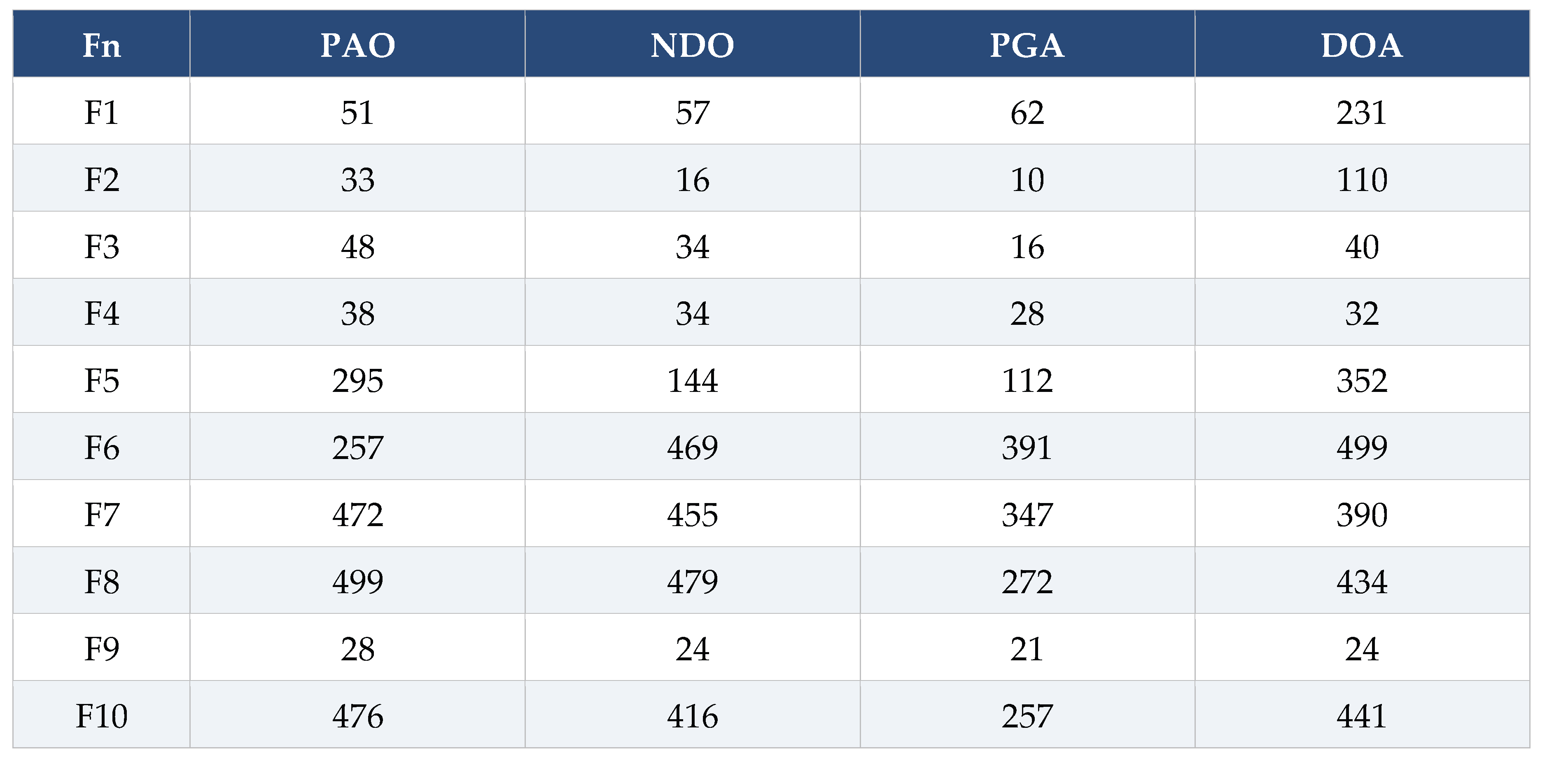 |
Table C6.
Runtime and global statistical-test summary for CEC-2019. Left: mean wall-clock time per run (averaged over the ten functions) and speed rank (1 = fastest of 43) for PAO and the leading optimizers. Right: omnibus and aggregate outcomes.
Table C6.
Runtime and global statistical-test summary for CEC-2019. Left: mean wall-clock time per run (averaged over the ten functions) and speed rank (1 = fastest of 43) for PAO and the leading optimizers. Right: omnibus and aggregate outcomes.
| Algorithm | Mean time / run (s) | Speed rank (of 43) |
| PAO | 2.2482 | 36 |
| NDO | 2.9266 | 40 |
| PGA | 4.0632 | 41 |
| DOA | 0.9896 | 12 |
| PSO | 0.9702 | 7 |
| GOA | 2.1007 | 34 |
Global statistical tests
| Test | Statistic | Outcome |
| Friedman omnibus (43 algorithms, 10 functions) | χ² = 228.86, df = 42 | p ≈ 1.5 × 10⁻²⁷ |
| Wilcoxon rank-sum, PAO vs all (aggregate) | 362 W / 31 T / 27 L | 86.2% win rate |
| PAO overall standing | mean rank 4.55 | 1st of 43 (NDO 2nd, 10.05) |
| Functions won by PAO | 3 of 10 ranked first | best rank 1, worst rank 11 (F6) |
Note. PAO’s first place on this suite is driven by broad consistency — top-six placement on eight of the ten functions — rather than by winning every function; it takes outright first place on F4, F5 and F9. Its limitations are localized to the Weierstrass function (F6) and the three specialized real-world problems (F1–F3).
Table C7.
Definition of the CEC-2019 “100-Digit Challenge” benchmark suite: for each of the ten functions, its name, dimension, search bounds and known global optimum. Functions CEC01–CEC03 carry their own dimensions (9, 16 and 18 variables respectively) and wide bounds; CEC04–CEC10 are all 10-dimensional on [−100, 100]. Every function has a global minimum value of 1, so results are reported as the gap above 1. Source:(Hamid et al., 2026; Price et al., 2018).
Table C7.
Definition of the CEC-2019 “100-Digit Challenge” benchmark suite: for each of the ten functions, its name, dimension, search bounds and known global optimum. Functions CEC01–CEC03 carry their own dimensions (9, 16 and 18 variables respectively) and wide bounds; CEC04–CEC10 are all 10-dimensional on [−100, 100]. Every function has a global minimum value of 1, so results are reported as the gap above 1. Source:(Hamid et al., 2026; Price et al., 2018).
| Function | Benchmark Function | Dimension | Lower/Upper Bound | Global Optimum (f(x^*)) |
| F1 | Storn’s Chebyshev Polynomial Fitting Problem | 9 | [-8192,8192] | 1 |
| F2 | Inverse Hilbert Matrix Problem | 16 | [-16384,16384] | 1 |
| F3 | Lennard-Jones Minimum Energy Cluster | 18 | [-4,4] | 1 |
| F4 | Rastrigin’s Function | 10 | [-100,100] | 1 |
| F5 | Griewank’s Function | 10 | [-100,100] | 1 |
| F6 | Weierstrass Function | 10 | [-100,100] | 1 |
| F7 | Modified Schwefel’s Function | 10 | [-100,100] | 1 |
| F8 | Expanded Schaffer’s F6 Function | 10 | [-100,100] | 1 |
| F9 | Happy Cat Function | 10 | [-100,100] | 1 |
| F10 | Ackley Function | 10 | [-100,100] | 1 |
Appendix D. Supporting Tables (CEC-2022)
All tables refer to the 43-algorithm comparison on the CEC-2022 suite at D = 10, 30 runs × 500 iterations, ranked on mean solution error f(x) − f*. Error values are reported in scientific E-notation.
Table D1.
Overall standing of all 43 algorithms on CEC-2022 (D = 10): mean rank over the twelve functions with overall position, and the number of functions on which each algorithm ranks first. PAO is first; GOA is a statistically level co-leader.
Table D1.
Overall standing of all 43 algorithms on CEC-2022 (D = 10): mean rank over the twelve functions with overall position, and the number of functions on which each algorithm ranks first. PAO is first; GOA is a statistically level co-leader.
| # | Algorithm | Mean rank | Functions won (rank 1) |
| 1 | PAO | 4.375 | 4 |
| 2 | GOA | 4.667 | 2 |
| 3 | APO | 5.833 | 2 |
| 4 | PGA | 8.708 | 0 |
| 5 | DOA | 9.083 | 2 |
| 6 | SFOA | 10.833 | 0 |
| 7 | NDO | 11.000 | 0 |
| 8 | EHO | 11.167 | 1 |
| 9 | SO | 12.500 | 0 |
| 10 | AOA | 13.083 | 0 |
| 11 | PSO | 13.417 | 0 |
| 12 | DHOLE | 13.583 | 0 |
| 13 | DE | 13.667 | 1 |
| 14 | CS | 13.833 | 0 |
| 15 | YDSE | 14.250 | 0 |
| 16 | HBA | 15.167 | 0 |
| 17 | SPIBA | 15.250 | 0 |
| 18 | FOA | 15.833 | 0 |
| 19 | WUTP | 17.083 | 0 |
| 20 | GWO | 20.250 | 0 |
| 21 | FPA | 20.917 | 0 |
| 22 | RFO | 21.333 | 0 |
| 23 | MSO | 21.833 | 0 |
| 24 | ZOA | 22.167 | 0 |
| 25 | AO | 23.333 | 0 |
| 26 | SHS | 23.500 | 0 |
| 27 | SOA | 24.417 | 0 |
| 28 | DSWO | 28.000 | 0 |
| 29 | WAA | 28.083 | 0 |
| 30 | MRSO | 28.167 | 0 |
| 31 | CPO | 29.250 | 0 |
| 32 | GOOSE | 30.833 | 0 |
| 33 | FOX | 31.083 | 0 |
| 34 | WSO | 31.583 | 0 |
| 35 | Chimp | 31.750 | 0 |
| 36 | TSO | 33.750 | 0 |
| 37 | HS | 33.917 | 0 |
| 38 | DRA | 36.917 | 0 |
| 39 | EMRA | 37.083 | 0 |
| 40 | SHO | 40.000 | 0 |
| 41 | MRA | 40.250 | 0 |
| 42 | CSA | 41.500 | 0 |
| 43 | DAOA | 42.750 | 0 |
Table D2.
PAO per-function performance on CEC-2022 (D = 10): mean, standard deviation and best solution error over 30 runs, with PAO’s rank among the 43 algorithms on that function. Function classes follow the suite definition.
Table D2.
PAO per-function performance on CEC-2022 (D = 10): mean, standard deviation and best solution error over 30 runs, with PAO’s rank among the 43 algorithms on that function. Function classes follow the suite definition.
| Fn | Benchmark function | Class | f* | PAO mean error | PAO std | PAO best | PAO rank |
| F1 | Shifted-Rotated Zakharov | Unimodal | 300 | 0.00 × 10⁰ | 1.06 × 10⁻¹⁴ | 0.00 × 10⁰ | 1 |
| F2 | Shifted-Rotated Rosenbrock | Basic multimodal | 400 | 6.81 × 10⁰ | 2.72 × 10⁰ | 0.00 × 10⁰ | 11 |
| F3 | Shifted-Rotated Expanded Schaffer F6 | Basic multimodal | 600 | 1.43 × 10⁻⁴ | 2.30 × 10⁻⁴ | 1.23 × 10⁻⁸ | 4 |
| F4 | Shifted-Rotated Non-Cont. Rastrigin | Basic multimodal | 800 | 2.69 × 10⁰ | 1.23 × 10⁰ | 0.00 × 10⁰ | 1 |
| F5 | Shifted-Rotated Levy | Basic multimodal | 900 | 0.00 × 10⁰ | 0.00 × 10⁰ | 0.00 × 10⁰ | 1 |
| F6 | Hybrid Function 1 | Hybrid | 1800 | 4.53 × 10⁻¹ | 2.70 × 10⁻¹ | 1.11 × 10⁻¹ | 1 |
| F7 | Hybrid Function 2 | Hybrid | 2000 | 9.84 × 10⁰ | 8.12 × 10⁰ | 2.02 × 10⁻⁸ | 3 |
| F8 | Hybrid Function 3 | Hybrid | 2200 | 1.33 × 10¹ | 7.53 × 10⁰ | 8.48 × 10⁻² | 2 |
| F9 | Composition Function 1 | Composition | 2300 | 2.29 × 10² | 0.00 × 10⁰ | 2.29 × 10² | 4.5 |
| F10 | Composition Function 2 | Composition | 2400 | 1.04 × 10² | 1.94 × 10¹ | 1.00 × 10² | 10 |
| F11 | Composition Function 3 | Composition | 2600 | 2.10 × 10² | 1.40 × 10² | 0.00 × 10⁰ | 9 |
| F12 | Composition Function 4 | Composition | 2700 | 1.62 × 10² | 1.23 × 10⁰ | 1.59 × 10² | 5 |
Table D3.
Mean solution error (standard deviation) over 30 runs for PAO and the five leading optimizers on CEC-2022 (D = 10), per function, with PAO’s per-function rank. Values in scientific E-notation.
Table D3.
Mean solution error (standard deviation) over 30 runs for PAO and the five leading optimizers on CEC-2022 (D = 10), per function, with PAO’s per-function rank. Values in scientific E-notation.
| Fn | PAO | GOA | APO | PGA | DOA | SFOA | PAO rank |
| F1 | 0.00 × 10⁰ (1.06 × 10⁻¹⁴) | 1.50 × 10⁻¹ (9.51 × 10⁻²) | 1.31 × 10⁻⁷ (1.29 × 10⁻⁷) | 1.08 × 10⁻² (4.95 × 10⁻²) | 3.15 × 10⁻² (1.56 × 10⁻¹) | 4.16 × 10⁻¹ (2.35 × 10⁻¹) | 1 |
| F2 | 6.81 × 10⁰ (2.72 × 10⁰) | 4.76 × 10⁻¹ (8.79 × 10⁻¹) | 3.99 × 10⁻¹ (1.22 × 10⁰) | 7.38 × 10⁰ (1.98 × 10⁰) | 1.37 × 10⁰ (2.42 × 10⁰) | 5.00 × 10⁰ (1.86 × 10⁰) | 11 |
| F3 | 1.43 × 10⁻⁴ (2.30 × 10⁻⁴) | 6.79 × 10⁻¹ (3.07 × 10⁻¹) | 1.42 × 10⁻³ (8.61 × 10⁻⁴) | 2.14 × 10⁻⁶ (9.01 × 10⁻⁶) | 5.11 × 10⁻³ (2.76 × 10⁻³) | 1.25 × 10⁰ (6.46 × 10⁻¹) | 4 |
| F4 | 2.69 × 10⁰ (1.23 × 10⁰) | 9.22 × 10⁰ (2.84 × 10⁰) | 2.19 × 10¹ (6.16 × 10⁰) | 1.45 × 10¹ (6.89 × 10⁰) | 1.84 × 10¹ (5.52 × 10⁰) | 3.26 × 10¹ (7.53 × 10⁰) | 1 |
| F5 | 0.00 × 10⁰ (0.00 × 10⁰) | 1.57 × 10⁻¹ (9.92 × 10⁻²) | 4.35 × 10⁻¹⁰ (7.60 × 10⁻¹⁰) | 3.20 × 10⁻⁹ (5.98 × 10⁻⁹) | 9.17 × 10⁰ (1.64 × 10¹) | 2.71 × 10⁰ (2.21 × 10⁰) | 1 |
| F6 | 4.53 × 10⁻¹ (2.70 × 10⁻¹) | 6.16 × 10⁰ (2.13 × 10⁰) | 5.46 × 10⁻¹ (2.51 × 10⁻¹) | 2.42 × 10³ (1.91 × 10³) | 2.72 × 10² (3.43 × 10²) | 2.73 × 10¹ (3.16 × 10¹) | 1 |
| F7 | 9.84 × 10⁰ (8.12 × 10⁰) | 1.22 × 10¹ (7.34 × 10⁰) | 1.22 × 10¹ (4.67 × 10⁰) | 1.87 × 10¹ (7.15 × 10⁰) | 6.39 × 10⁰ (9.03 × 10⁰) | 2.38 × 10¹ (3.10 × 10⁰) | 3 |
| F8 | 1.33 × 10¹ (7.53 × 10⁰) | 5.52 × 10⁰ (2.70 × 10⁰) | 1.57 × 10¹ (4.33 × 10⁰) | 2.08 × 10¹ (3.85 × 10⁰) | 1.59 × 10¹ (7.30 × 10⁰) | 2.13 × 10¹ (6.33 × 10⁰) | 2 |
| F9 | 2.29 × 10² (0.00 × 10⁰) | 2.25 × 10² (2.27 × 10¹) | 2.29 × 10² (2.88 × 10⁻⁵) | 2.29 × 10² (0.00 × 10⁰) | 2.29 × 10² (2.95 × 10⁻⁴) | 2.29 × 10² (2.11 × 10⁻⁹) | 4.5 |
| F10 | 1.04 × 10² (1.94 × 10¹) | 1.00 × 10² (4.26 × 10⁻²) | 1.00 × 10² (4.91 × 10⁻²) | 1.08 × 10² (2.95 × 10¹) | 5.15 × 10¹ (5.80 × 10¹) | 1.00 × 10² (8.77 × 10⁻²) | 10 |
| F11 | 2.10 × 10² (1.40 × 10²) | 1.34 × 10¹ (5.44 × 10¹) | 6.68 × 10⁻⁵ (3.24 × 10⁻⁵) | 7.17 × 10¹ (1.38 × 10²) | 2.51 × 10² (9.15 × 10¹) | 2.87 × 10¹ (7.18 × 10¹) | 9 |
| F12 | 1.62 × 10² (1.23 × 10⁰) | 1.60 × 10² (7.83 × 10⁻¹) | 1.64 × 10² (1.10 × 10⁰) | 1.64 × 10² (8.99 × 10⁻¹) | 1.65 × 10² (1.61 × 10⁰) | 1.60 × 10² (1.05 × 10⁰) | 5 |
Table D4.
PAO versus each competitor on CEC-2022 (12 functions, D = 10): Wilcoxon rank-sum wins (W), ties (T) and losses (L) for PAO, with net score (W−L). Sorted from PAO’s largest advantage. Aggregate: 445 W / 32 T / 27 L (88.3% win rate). Note the even split with GOA.
Table D4.
PAO versus each competitor on CEC-2022 (12 functions, D = 10): Wilcoxon rank-sum wins (W), ties (T) and losses (L) for PAO, with net score (W−L). Sorted from PAO’s largest advantage. Aggregate: 445 W / 32 T / 27 L (88.3% win rate). Note the even split with GOA.
| Competitor | W | T | L | Net | Competitor | W | T | L | Net | |
| AOA | 12 | 0 | 0 | +12 | FOX | 11 | 1 | 0 | +11 | |
| CPO | 12 | 0 | 0 | +12 | GOOSE | 11 | 1 | 0 | +11 | |
| CSA | 12 | 0 | 0 | +12 | MSO | 11 | 1 | 0 | +11 | |
| Chimp | 12 | 0 | 0 | +12 | PSO | 11 | 1 | 0 | +11 | |
| DAOA | 12 | 0 | 0 | +12 | RFO | 11 | 1 | 0 | +11 | |
| DRA | 12 | 0 | 0 | +12 | FPA | 11 | 0 | 1 | +10 | |
| DSWO | 12 | 0 | 0 | +12 | SO | 11 | 0 | 1 | +10 | |
| EMRA | 12 | 0 | 0 | +12 | SPIBA | 11 | 0 | 1 | +10 | |
| FOA | 12 | 0 | 0 | +12 | DHOLE | 10 | 2 | 0 | +10 | |
| GWO | 12 | 0 | 0 | +12 | HBA | 10 | 2 | 0 | +10 | |
| HS | 12 | 0 | 0 | +12 | WUTP | 10 | 2 | 0 | +10 | |
| MRA | 12 | 0 | 0 | +12 | NDO | 8 | 4 | 0 | +8 | |
| MRSO | 12 | 0 | 0 | +12 | DOA | 8 | 3 | 1 | +7 | |
| SHO | 12 | 0 | 0 | +12 | YDSE | 8 | 3 | 1 | +7 | |
| SHS | 12 | 0 | 0 | +12 | EHO | 9 | 0 | 3 | +6 | |
| SOA | 12 | 0 | 0 | +12 | CS | 8 | 1 | 3 | +5 | |
| TSO | 12 | 0 | 0 | +12 | PGA | 8 | 1 | 3 | +5 | |
| WAA | 12 | 0 | 0 | +12 | SFOA | 8 | 1 | 3 | +5 | |
| WSO | 12 | 0 | 0 | +12 | DE | 7 | 3 | 2 | +5 | |
| ZOA | 12 | 0 | 0 | +12 | APO | 7 | 2 | 3 | +4 | |
| AO | 11 | 1 | 0 | +11 | GOA | 5 | 2 | 5 | +0 |
Table D5.
Effective convergence iteration on CEC-2022 (the iteration at which the mean best-so-far error first reaches within 1% of its terminal value) for PAO and three leading optimizers, per function. Lower means faster stabilization.
Table D5.
Effective convergence iteration on CEC-2022 (the iteration at which the mean best-so-far error first reaches within 1% of its terminal value) for PAO and three leading optimizers, per function. Lower means faster stabilization.
| Fn | PAO | GOA | APO | PGA |
| F1 | 95 | 88 | 136 | 160 |
| F2 | 45 | 118 | 131 | 22 |
| F3 | 103 | 442 | 258 | 40 |
| F4 | 324 | 466 | 485 | 104 |
| F5 | 59 | 139 | 119 | 23 |
| F6 | 16 | 20 | 22 | 14 |
| F7 | 390 | 481 | 470 | 76 |
| F8 | 405 | 479 | 429 | 101 |
| F9 | 48 | 198 | 186 | 24 |
| F10 | 35 | 37 | 49 | 17 |
| F11 | 45 | 41 | 82 | 23 |
| F12 | 80 | 338 | 248 | 22 |
Table D6.
Runtime and global statistical-test summary for CEC-2022 (D = 10). Left: mean wall-clock time per run (averaged over the twelve functions) and speed rank (1 = fastest of 43) for PAO and the leading optimizers. Right: omnibus and aggregate outcomes.
Table D6.
Runtime and global statistical-test summary for CEC-2022 (D = 10). Left: mean wall-clock time per run (averaged over the twelve functions) and speed rank (1 = fastest of 43) for PAO and the leading optimizers. Right: omnibus and aggregate outcomes.
| Algorithm | Mean time / run (s) | Speed rank (of 43) |
| PAO | 1.8046 | 41 |
| GOA | 0.3932 | 30 |
| APO | 1.1197 | 38 |
| PGA | 0.8414 | 36 |
| DOA | 0.1291 | 9 |
| SFOA | 0.1152 | 4 |
Global statistical tests
| Test | Statistic | Outcome |
| Friedman omnibus (43 algorithms, 12 functions) | χ² = 378.08, df = 42 | p ≈ 1.2 × 10⁻⁵⁵ |
| Wilcoxon rank-sum, PAO vs all (aggregate) | 445 W / 32 T / 27 L | 88.3% win rate |
| PAO overall standing | mean rank 4.375 | 1st of 43 (GOA 2nd, 4.667) |
| PAO vs GOA (head-to-head) | 5 W / 2 T / 5 L | even — co-leaders |
| Functions won by PAO | 4 of 12 ranked first | best rank 1, worst rank 11 (F2) |
Note. These results are for D = 10; the suite is also defined at D = 20. PAO’s first place is genuine but narrow — GOA is a statistically level co-leader (even head-to-head record) — and is earned by solving the unimodal, basic-multimodal and hybrid functions to the optimum, several on every run. Its weaknesses are the Rosenbrock function (F2) and two composition functions (F10, F11).
Table D7.
Definition of the CEC-2022 benchmark suite: for each of the twelve functions, its class, name, dimension, search bounds and known global optimum. The suite comprises one unimodal, four basic multimodal, three hybrid and four composition functions on [−100, 100]^D, run here at D = 10 and D = 20. Source:(Salgotra et al., 2025).
Table D7.
Definition of the CEC-2022 benchmark suite: for each of the twelve functions, its class, name, dimension, search bounds and known global optimum. The suite comprises one unimodal, four basic multimodal, three hybrid and four composition functions on [−100, 100]^D, run here at D = 10 and D = 20. Source:(Salgotra et al., 2025).
| Function | Type | Benchmark Function | Dimension | Lower/Upper Bound | Global Optimum (f(x^*)) |
| F1 | Unimodal | Shifted & Rotated Zakharov | 10 | [-100,100] | 300 |
| F2 | Basic | Shifted & Rotated Rosenbrock | 10 | [-100,100] | 400 |
| F3 | Basic | Shifted & Rotated Expanded Schaffer’s F6 | 10 | [-100,100] | 600 |
| F4 | Basic | Shifted & Rotated Non-Continuous Rastrigin | 10 | [-100,100] | 800 |
| F5 | Basic | Shifted & Rotated Levy | 10 | [-100,100] | 900 |
| F6 | Hybrid | Hybrid Function 1 | 10 | [-100,100] | 1800 |
| F7 | Hybrid | Hybrid Function 2 | 10 | [-100,100] | 2000 |
| F8 | Hybrid | Hybrid Function 3 | 10 | [-100,100] | 2200 |
| F9 | Composite | Composition Function 1 | 10 | [-100,100] | 2300 |
| F10 | Composite | Composition Function 2 | 10 | [-100,100] | 2400 |
| F11 | Composite | Composition Function 3 | 10 | [-100,100] | 2600 |
| F12 | Composite | Composition Function 4 | 10 | [-100,100] | 2700 |
Appendix E. Qualitative Analysis — Full Per-Function Results
Five-panel qualitative composites for PAO on the remaining classical benchmark functions (two-dimensional form), followed by the per-function exploration/exploitation curves and a comparison of PAO’s exploration percentage against the 43-algorithm field. Each composite shows, left to right: the landscape, the search history of all agents, the trajectory of the first agent, the population-average fitness, and the convergence curve.
Figure E.1.
Qualitative analysis of PAO on F2 (2-D): landscape, search history, trajectory, population-average
fitness and convergence.
Figure E.1.
Qualitative analysis of PAO on F2 (2-D): landscape, search history, trajectory, population-average
fitness and convergence.
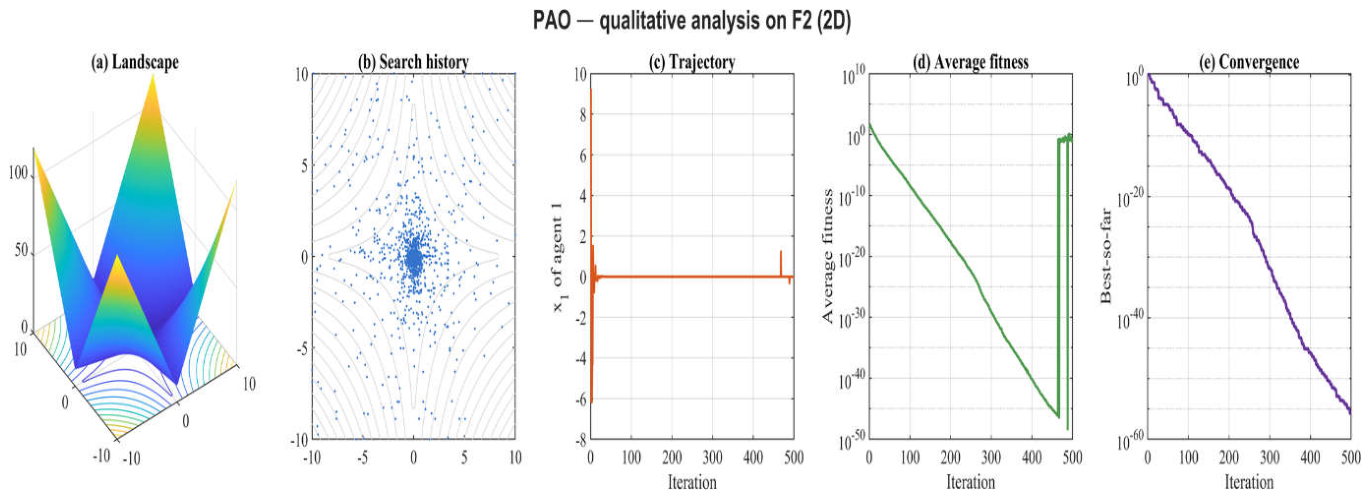
Figure E.2.
Qualitative analysis of PAO on F3 (2-D): landscape, search history, trajectory, population-average
fitness and convergence.
Figure E.2.
Qualitative analysis of PAO on F3 (2-D): landscape, search history, trajectory, population-average
fitness and convergence.
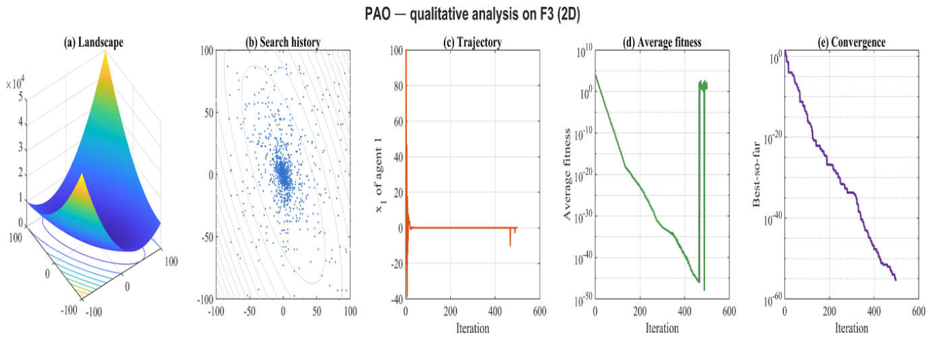
Figure E.3.
Qualitative analysis of PAO on F4 (2-D): landscape, search history, trajectory, population-average
fitness and convergence.
Figure E.3.
Qualitative analysis of PAO on F4 (2-D): landscape, search history, trajectory, population-average
fitness and convergence.
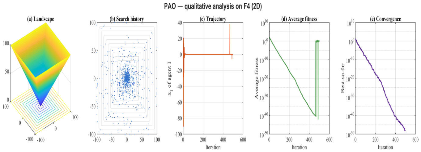
Figure E.4.
Qualitative analysis of PAO on F5 (2-D): landscape, search history, trajectory, population-average
fitness and convergence.
Figure E.4.
Qualitative analysis of PAO on F5 (2-D): landscape, search history, trajectory, population-average
fitness and convergence.
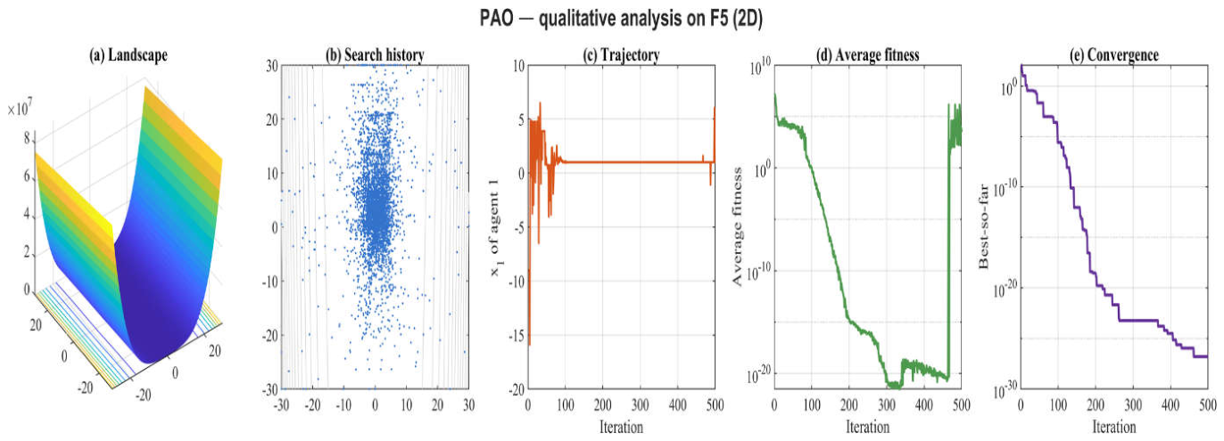
Figure E.5.
Qualitative analysis of PAO on F6 (2-D): landscape, search history, trajectory, population-average
fitness and convergence.
Figure E.5.
Qualitative analysis of PAO on F6 (2-D): landscape, search history, trajectory, population-average
fitness and convergence.
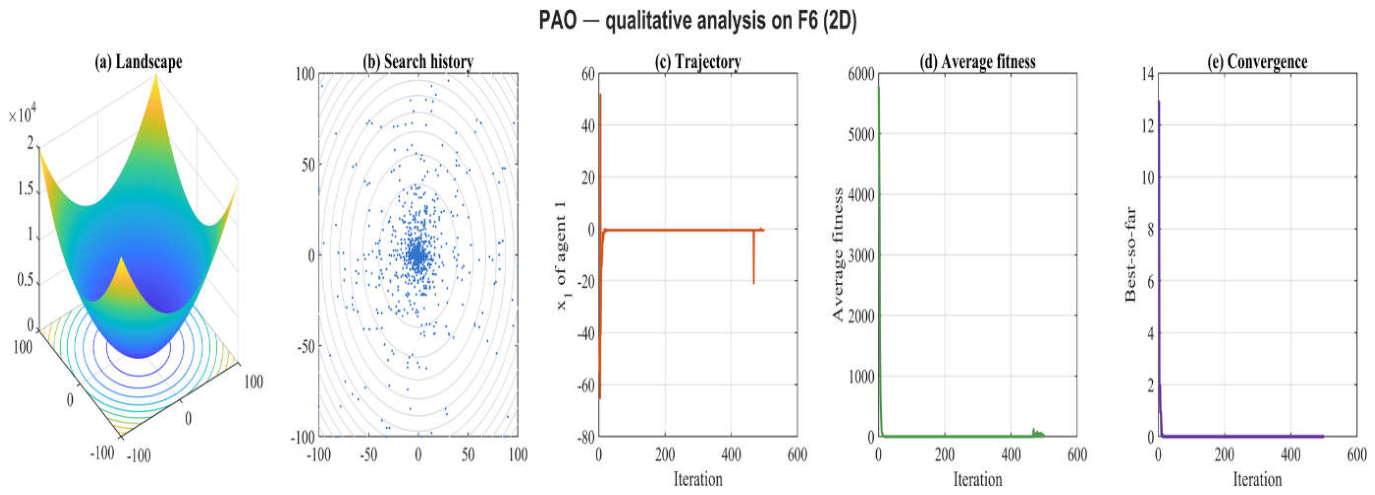
Figure E.6.
Qualitative analysis of PAO on F7 (2-D): landscape, search history, trajectory, population-average
fitness and convergence.
Figure E.6.
Qualitative analysis of PAO on F7 (2-D): landscape, search history, trajectory, population-average
fitness and convergence.
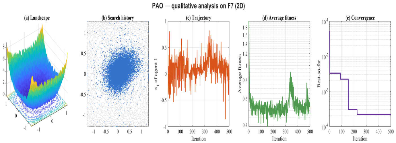
Figure E.7.
Qualitative analysis of PAO on F8 (2-D): landscape, search history, trajectory, population-average
fitness and convergence.
Figure E.7.
Qualitative analysis of PAO on F8 (2-D): landscape, search history, trajectory, population-average
fitness and convergence.
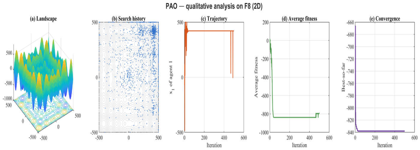
Figure E.8.
Qualitative analysis of PAO on F10 (2-D): landscape, search history, trajectory, population-average
fitness and convergence.
Figure E.8.
Qualitative analysis of PAO on F10 (2-D): landscape, search history, trajectory, population-average
fitness and convergence.
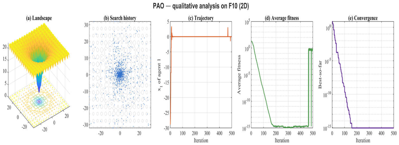
Figure E.9.
Qualitative analysis of PAO on F11 (2-D): landscape, search history, trajectory, population-average
fitness and convergence.
Figure E.9.
Qualitative analysis of PAO on F11 (2-D): landscape, search history, trajectory, population-average
fitness and convergence.
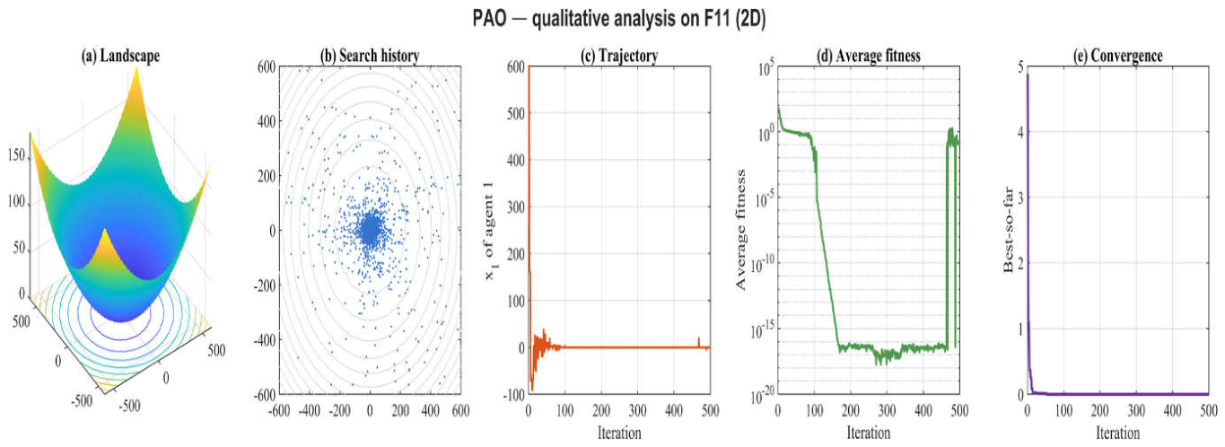
Figure E.10.
Qualitative analysis of PAO on F12 (2-D): landscape, search history, trajectory, population-average
fitness and convergence.
Figure E.10.
Qualitative analysis of PAO on F12 (2-D): landscape, search history, trajectory, population-average
fitness and convergence.
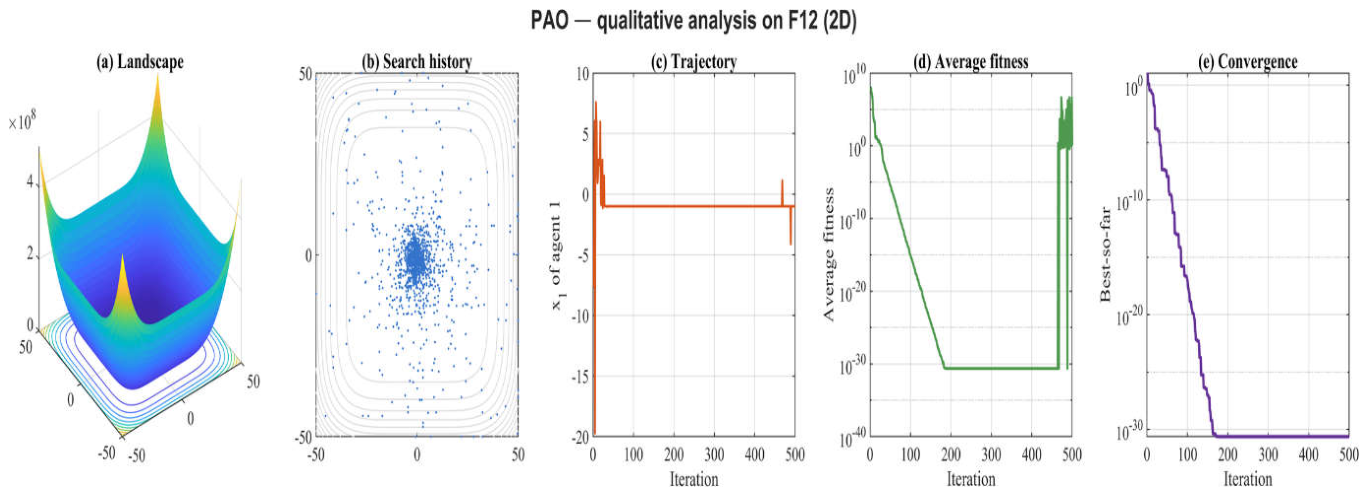
Figure E.11.
Qualitative analysis of PAO on F13 (2-D): landscape, search history, trajectory, population-average
fitness and convergence.
Figure E.11.
Qualitative analysis of PAO on F13 (2-D): landscape, search history, trajectory, population-average
fitness and convergence.
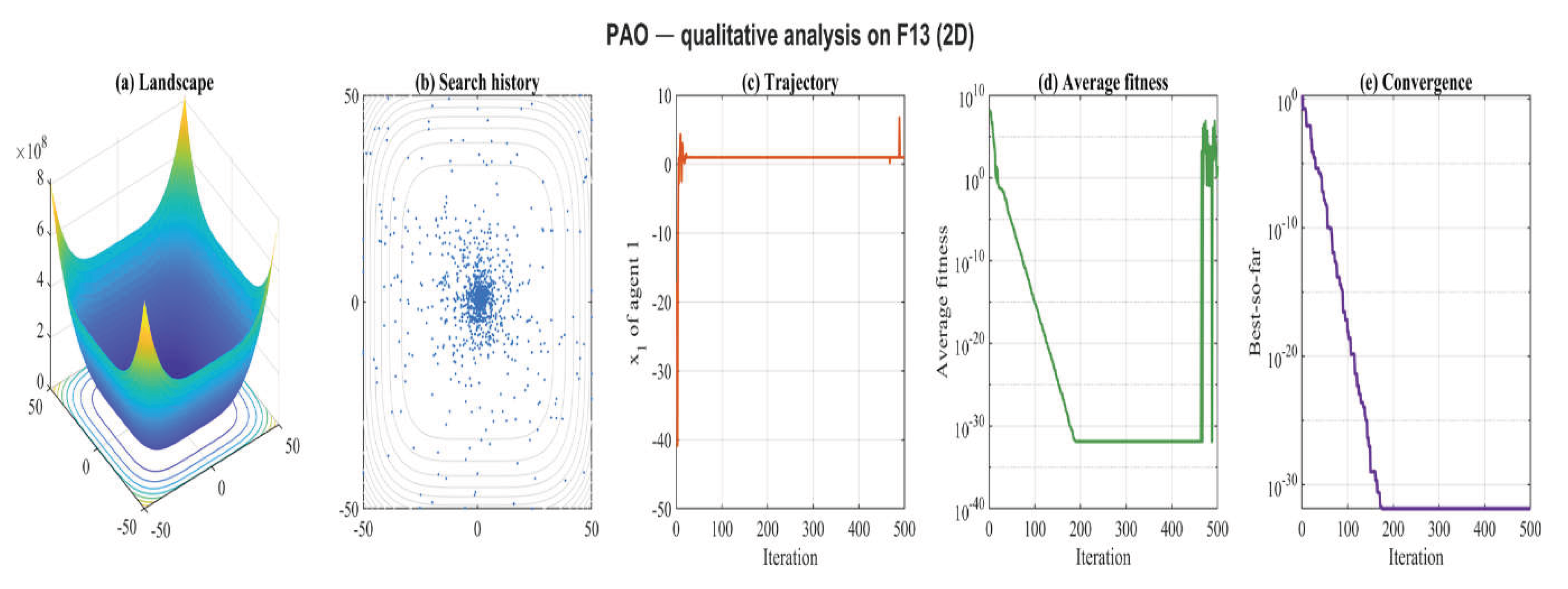
Figure E.12.
Qualitative analysis of PAO on F14 (2-D): landscape, search history, trajectory, population-average
fitness and convergence.
Figure E.12.
Qualitative analysis of PAO on F14 (2-D): landscape, search history, trajectory, population-average
fitness and convergence.
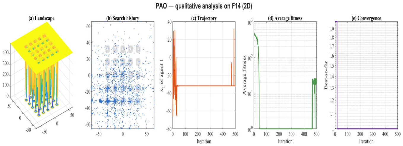
Figure E.13.
Qualitative analysis of PAO on F16 (2-D): landscape, search history, trajectory, population-average
fitness and convergence.
Figure E.13.
Qualitative analysis of PAO on F16 (2-D): landscape, search history, trajectory, population-average
fitness and convergence.
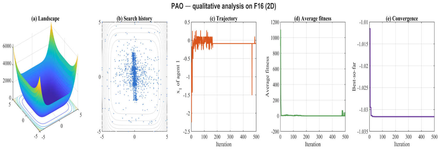
Figure E.14.
Qualitative analysis of PAO on F17 (2-D): landscape, search history, trajectory, population-average
fitness and convergence.
Figure E.14.
Qualitative analysis of PAO on F17 (2-D): landscape, search history, trajectory, population-average
fitness and convergence.
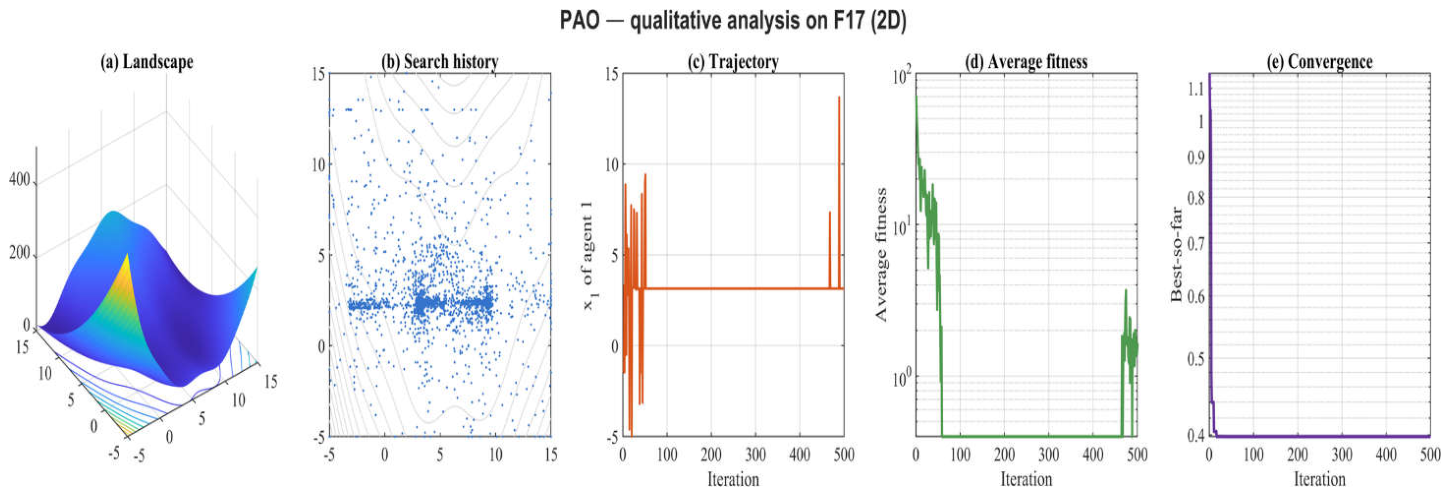
Figure E.15.
Qualitative analysis of PAO on F18 (2-D): landscape, search history, trajectory, population-average
fitness and convergence.
Figure E.15.
Qualitative analysis of PAO on F18 (2-D): landscape, search history, trajectory, population-average
fitness and convergence.
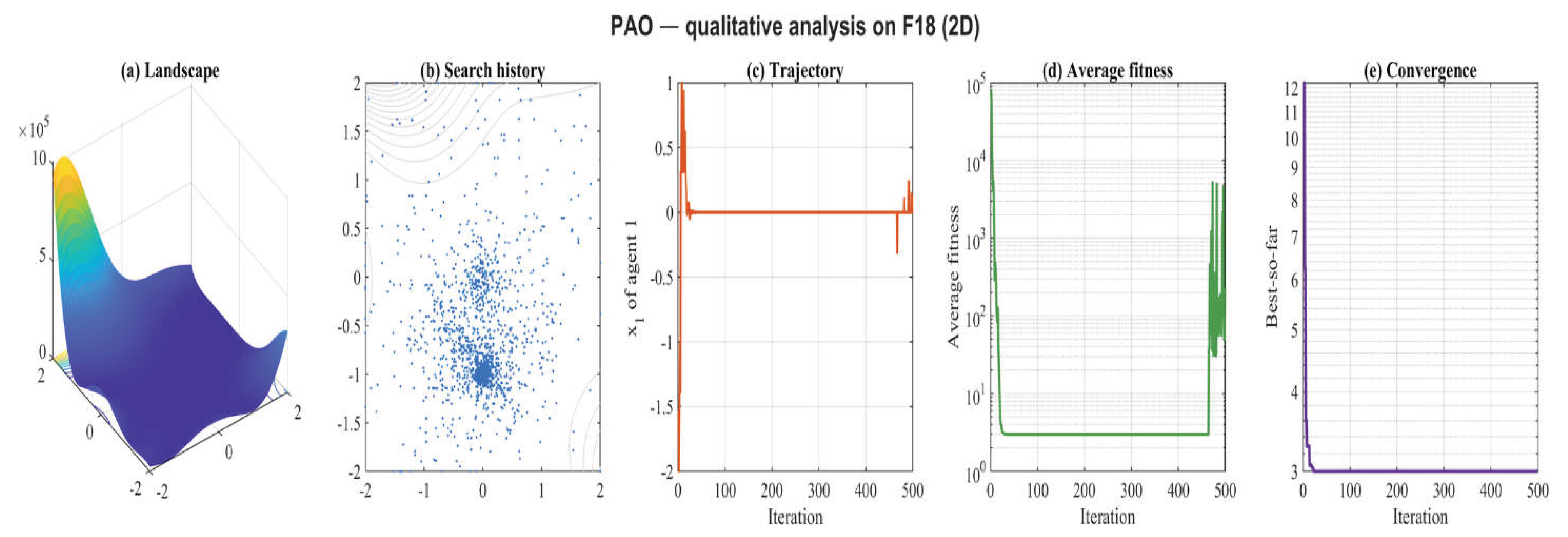
Exploration/exploitation curves. Per-iteration exploration (%) and exploitation (%) for PAO on the five functions of Table 10, derived from dimension-wise population diversity.
Figure E.16.
PAO per-iteration exploration/exploitation on F1 (Sphere (unimodal)).
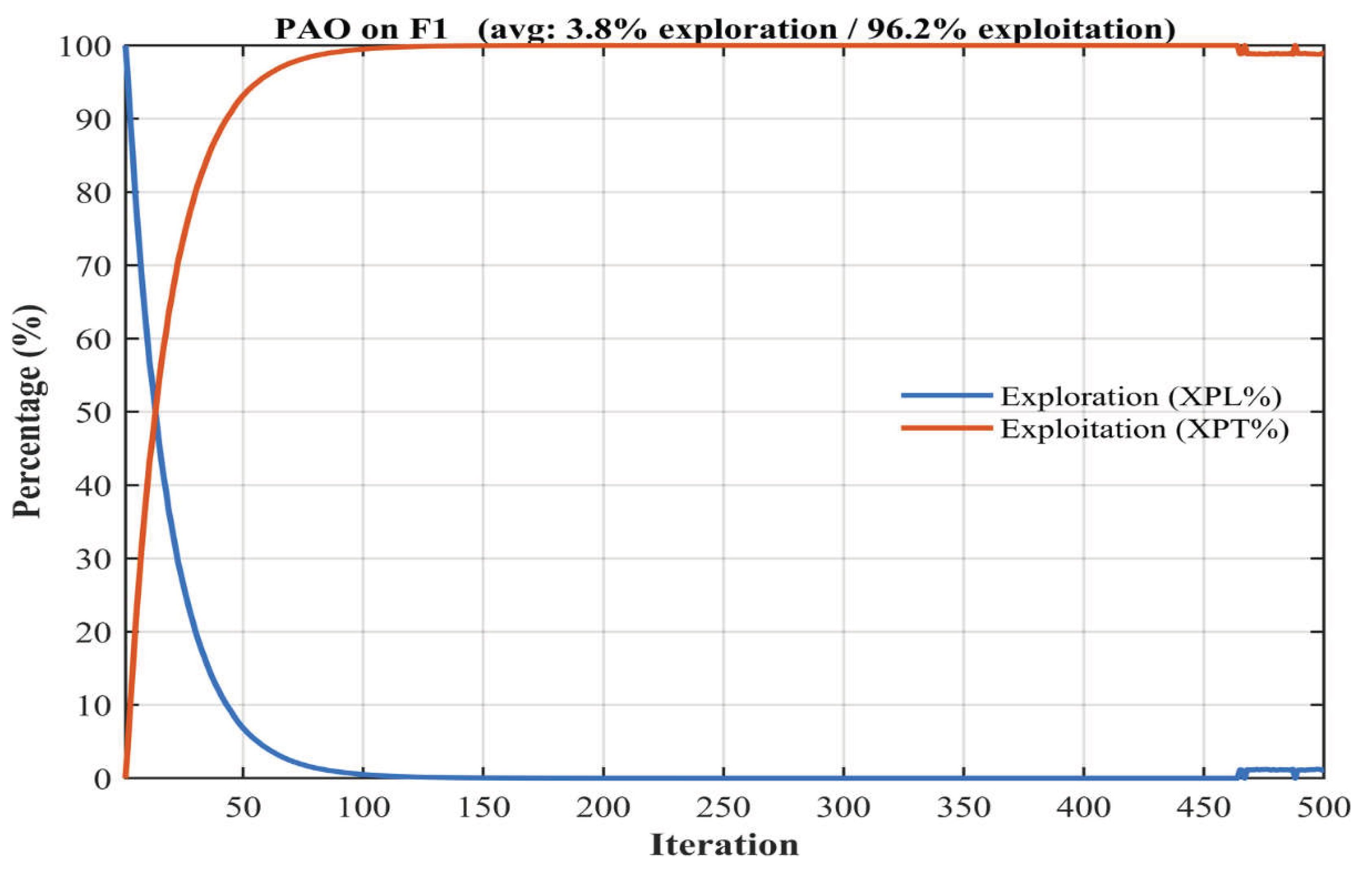
Figure E.17.
PAO per-iteration exploration/exploitation on F7 (Quartic + noise (unimodal)).
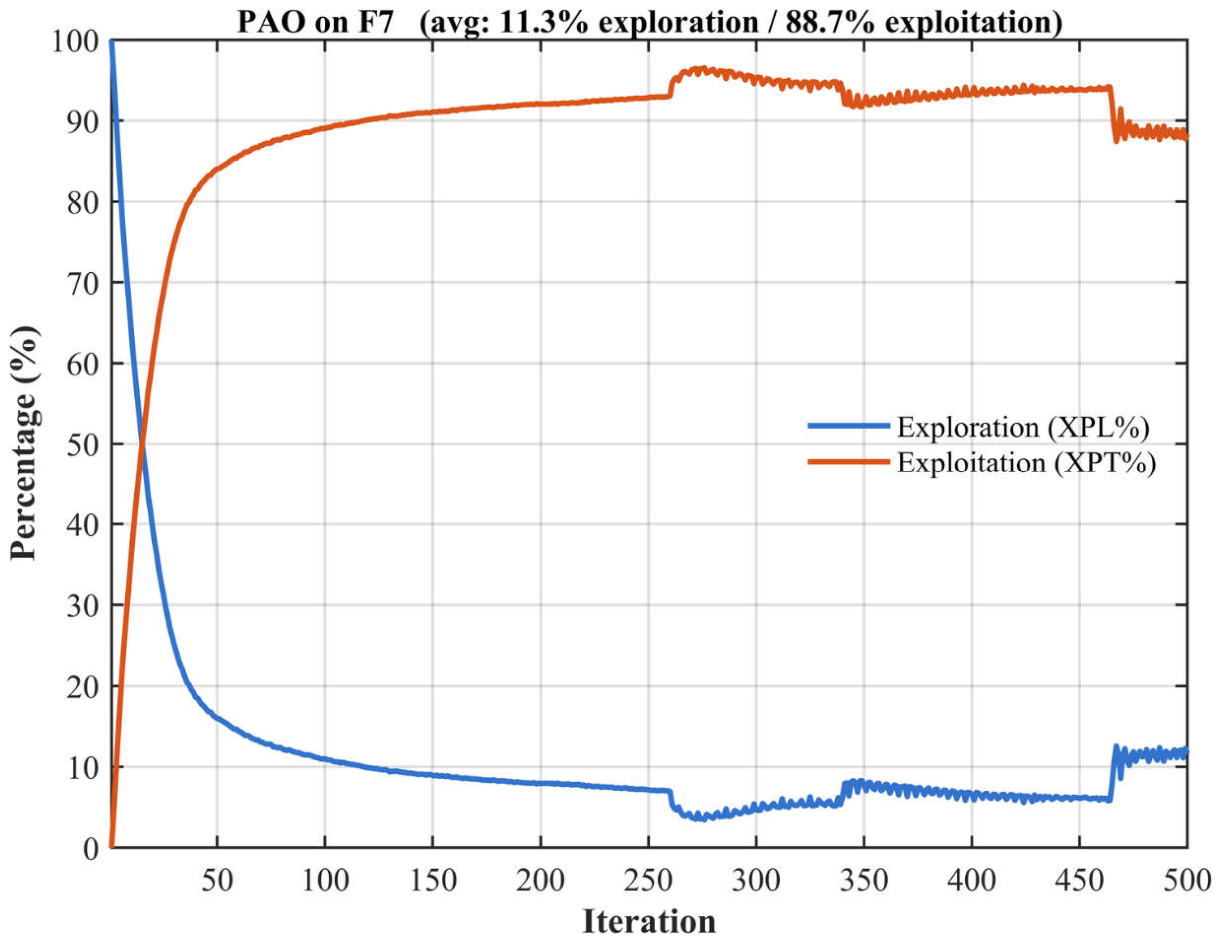
Figure E.18.
PAO per-iteration exploration/exploitation on F8 (Schwefel 2.26 (multimodal)).
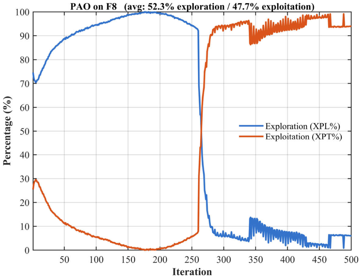
Figure E.19.
PAO per-iteration exploration/exploitation on F15 (Kowalik (fixed-dimension)).
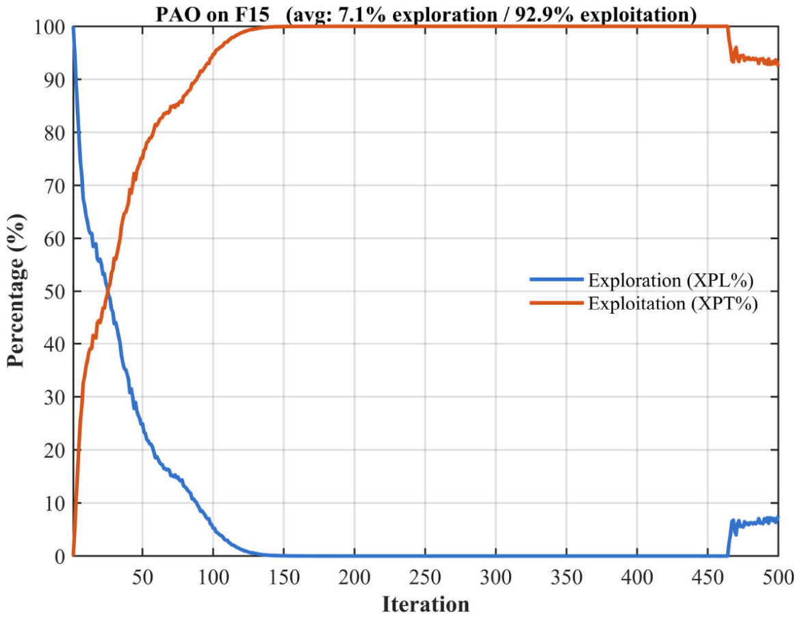
Figure E.20.
PAO per-iteration exploration/exploitation on F19 (Hartman 3 (fixed-dimension)).
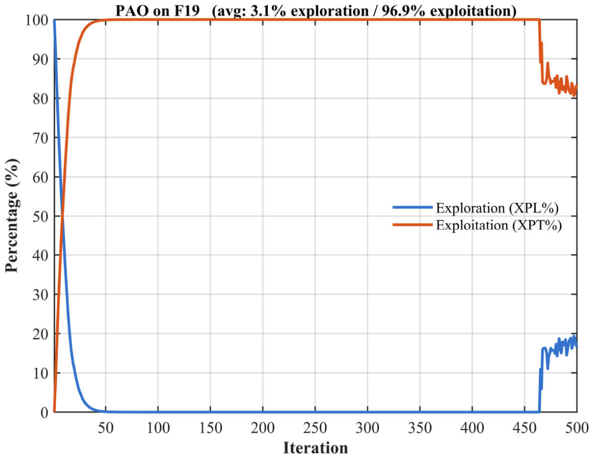
Table E1.
PAO run-averaged exploration percentage against the 43-algorithm field on the five functions. The field minimum and maximum show the full spread of search regimes among the compared algorithms; PAO sits near the exploitative (low-exploration) end except on the deceptive Schwefel function (F8).
Table E1.
PAO run-averaged exploration percentage against the 43-algorithm field on the five functions. The field minimum and maximum show the full spread of search regimes among the compared algorithms; PAO sits near the exploitative (low-exploration) end except on the deceptive Schwefel function (F8).
| Fn | Function | PAO exploration % | Field mean % | Field min % | Field max % |
| F1 | Sphere | 3.8 | 13.1 | 0.4 | 73.1 |
| F7 | Quartic+noise | 11.3 | 24.4 | 0.7 | 76.6 |
| F8 | Schwefel 2.26 | 52.3 | 47.0 | 0.7 | 98.9 |
| F15 | Kowalik | 7.1 | 28.4 | 1.3 | 89.6 |
| F19 | Hartman 3 | 3.1 | 32.9 | 0.9 | 80.1 |
Appendix F. Statistical Analysis — Detailed Results
Supporting detail for Section 5.8: the critical differences produced by the two standard post-hoc procedures, and the number of competitors PAO significantly outperforms under each.
Table F1.
Post-hoc critical differences on each suite. The Nemenyi CD applies to all pairwise comparisons; the Bonferroni–Dunn CD applies to comparisons against a single control (PAO) and is therefore tighter. “Not separated” counts the algorithms lying within the Bonferroni–Dunn CD of PAO — a consequence of correcting for 42 comparisons, not of comparable performance.
Table F1.
Post-hoc critical differences on each suite. The Nemenyi CD applies to all pairwise comparisons; the Bonferroni–Dunn CD applies to comparisons against a single control (PAO) and is therefore tighter. “Not separated” counts the algorithms lying within the Bonferroni–Dunn CD of PAO — a consequence of correcting for 42 comparisons, not of comparable performance.
| Suite | Nemenyi CD (α = 0.05) | Bonferroni–Dunn CD | Algorithms not separated from PAO | PAO significantly better (Holm) |
| Classical-23 | 14.52 | 12.00 | 29 of 42 | 13 of 42 |
| CEC-2017 | 12.71 | 10.51 | 9 of 42 | 34 of 42 |
| CEC-2019 | 22.02 | 18.20 | 24 of 42 | 19 of 42 |
| CEC-2022 | 20.10 | 16.61 | 20 of 42 | 24 of 42 |
Note. The Friedman and Wilcoxon results reported in Table 11 are reproduced from the per-suite analyses of Section 5.1, Section 5.2, Section 5.3 and Section 5.4, where they are derived and discussed in the context of each benchmark. The wide critical differences above are a property of the experimental design — 43 algorithms compared over between 10 and 30 functions — and should be interpreted as a conservative bound rather than as evidence of equivalence.
Appendix G. Scalability — Detailed Results
Table G1.
PAO mean solution error on the thirteen scalable classical functions at each dimension (30 runs, 500 iterations, N = 60). F8 is the Schwefel 2.26 function, whose optimum scales with D and which is therefore reported separately in Table G3.
Table G1.
PAO mean solution error on the thirteen scalable classical functions at each dimension (30 runs, 500 iterations, N = 60). F8 is the Schwefel 2.26 function, whose optimum scales with D and which is therefore reported separately in Table G3.
| Fn | D = 10 | D = 20 | D = 30 | D = 50 | D = 100 |
| F1 | 2.54 × 10⁻²⁶ | 1.09 × 10⁻¹⁸ | 4.22 × 10⁻¹² | 3.27 × 10⁻⁵ | 4.72 × 10⁰ |
| F2 | 6.41 × 10⁻¹⁸ | 1.52 × 10⁻¹⁰ | 2.10 × 10⁻⁷ | 1.70 × 10⁻³ | 9.10 × 10⁻¹ |
| F3 | 2.21 × 10⁻¹⁸ | 8.85 × 10⁻⁵ | 1.41 × 10⁰ | 2.72 × 10² | 5.37 × 10³ |
| F4 | 4.48 × 10⁻¹² | 5.22 × 10⁻² | 2.34 × 10⁰ | 1.07 × 10¹ | 1.77 × 10¹ |
| F5 | 3.00 × 10⁻⁶ | 9.86 × 10⁰ | 2.37 × 10¹ | 1.23 × 10² | 1.84 × 10³ |
| F6 | 2.08 × 10⁻²⁶ | 1.18 × 10⁻¹⁸ | 2.17 × 10⁻¹² | 3.82 × 10⁻⁵ | 5.00 × 10⁰ |
| F7 | 1.23 × 10⁻³ | 3.37 × 10⁻³ | 5.97 × 10⁻³ | 3.13 × 10⁻² | 3.52 × 10⁻¹ |
| F8 | -4.18 × 10³ | -8.24 × 10³ | -1.03 × 10⁴ | -1.34 × 10⁴ | -2.08 × 10⁴ |
| F9 | 0.00 × 10⁰ | 3.32 × 10⁻² | 8.95 × 10⁻¹ | 8.76 × 10⁰ | 5.91 × 10¹ |
| F10 | 4.44 × 10⁻¹⁵ | 1.10 × 10⁻¹⁰ | 4.45 × 10⁻⁷ | 1.24 × 10⁰ | 3.19 × 10⁰ |
| F11 | 2.55 × 10⁻³ | 4.11 × 10⁻⁴ | 2.05 × 10⁻³ | 8.57 × 10⁻³ | 9.49 × 10⁻¹ |
| F12 | 1.02 × 10⁻²⁶ | 1.28 × 10⁻¹⁸ | 3.46 × 10⁻³ | 3.23 × 10⁻² | 1.88 × 10⁰ |
| F13 | 2.57 × 10⁻²⁶ | 1.82 × 10⁻¹⁸ | 5.16 × 10⁻¹² | 1.48 × 10⁻¹ | 9.83 × 10¹ |
Table G2.
PAO mean solution error on the CEC-2022 suite at D = 10 and D = 20, with the ratio between them. Values are errors above the known optimum; a ratio below 1 indicates the higher dimension gave the lower error.
Table G2.
PAO mean solution error on the CEC-2022 suite at D = 10 and D = 20, with the ratio between them. Values are errors above the known optimum; a ratio below 1 indicates the higher dimension gave the lower error.
| Fn | Error at D = 10 | Error at D = 20 | Ratio D20 / D10 |
| F1 | 0.00 × 10⁰ | 1.63 × 10¹ | -- |
| F2 | 7.44 × 10⁰ | 4.89 × 10¹ | 6.58 |
| F3 | 1.92 × 10⁻⁴ | 3.73 × 10⁻³ | 19.40 |
| F4 | 3.02 × 10⁰ | 1.03 × 10¹ | 3.42 |
| F5 | 0.00 × 10⁰ | 1.79 × 10⁻² | -- |
| F6 | 4.31 × 10⁻¹ | 6.87 × 10¹ | 159.24 |
| F7 | 8.53 × 10⁰ | 3.96 × 10¹ | 4.64 |
| F8 | 1.42 × 10¹ | 2.52 × 10¹ | 1.78 |
| F9 | 2.29 × 10² | 1.81 × 10² | 0.79 |
| F10 | 1.07 × 10² | 1.02 × 10² | 0.95 |
| F11 | 2.60 × 10² | 3.00 × 10² | 1.15 |
| F12 | 1.61 × 10² | 2.37 × 10² | 1.47 |
Table G3.
Schwefel 2.26 (F8) across dimensions, expressed as the percentage of the dimension-dependent optimum f* = −418.98 D attained by PAO. This is the clearest case of dimensional degradation observed in the study.
Table G3.
Schwefel 2.26 (F8) across dimensions, expressed as the percentage of the dimension-dependent optimum f* = −418.98 D attained by PAO. This is the clearest case of dimensional degradation observed in the study.
| Dimension D | PAO mean | Optimum f* | Percentage of optimum attained |
| D = 10 | -4178.0 | -4189.8 | 99.7% |
| D = 20 | -8237.5 | -8379.7 | 98.3% |
| D = 30 | -10271.2 | -12569.5 | 81.7% |
| D = 50 | -13364.7 | -20949.1 | 63.8% |
| D = 100 | -20839.0 | -41898.3 | 49.7% |
Appendix H. Population-size Sensitivity — Detailed Results
Per-function results underlying the population-size study of Section 5.10. PAO was run at each N ∈ {10, 20, 30, 50, 60} on the CEC-2019 suite (ten functions, 30 runs, 500 iterations). Values are the solution error (f − 1, the objective gap above the optimum value of 1) in scientific E-notation. The best (lowest) entry in each row is highlighted.
Table H1.
Mean solution error of PAO over 30 runs at each population size N, per CEC-2019 function. Lowest error in each row highlighted; F2 and F3 are population-independent.
Table H1.
Mean solution error of PAO over 30 runs at each population size N, per CEC-2019 function. Lowest error in each row highlighted; F2 and F3 are population-independent.
| Fn | Benchmark function | N = 10 | N = 20 | N = 30 | N = 50 | N = 60 |
| F1 | Chebyshev (9D) | 1.09 × 10⁹ | 2.43 × 10⁷ | 8.12 × 10⁵ | 8.94 × 10⁴ | 3.14 × 10⁴ |
| F2 | Inverse Hilbert (16D) | 1.73 × 10¹ | 1.73 × 10¹ | 1.73 × 10¹ | 1.73 × 10¹ | 1.73 × 10¹ |
| F3 | Lennard-Jones (18D) | 1.27 × 10¹ | 1.27 × 10¹ | 1.27 × 10¹ | 1.27 × 10¹ | 1.27 × 10¹ |
| F4 | Rastrigin (10D) | 4.61 × 10¹ | 8.17 × 10⁰ | 4.38 × 10⁰ | 2.92 × 10⁰ | 1.99 × 10⁰ |
| F5 | Griewank (10D) | 1.10 × 10⁰ | 1.02 × 10⁰ | 1.01 × 10⁰ | 1.01 × 10⁰ | 1.00 × 10⁰ |
| F6 | Weierstrass (10D) | 8.59 × 10⁰ | 8.30 × 10⁰ | 8.24 × 10⁰ | 8.13 × 10⁰ | 8.05 × 10⁰ |
| F7 | Modified Schwefel (10D) | 2.05 × 10² | 1.29 × 10² | 1.19 × 10² | 7.05 × 10¹ | 6.89 × 10¹ |
| F8 | Exp. Schaffer F6 (10D) | 4.50 × 10⁰ | 4.03 × 10⁰ | 3.50 × 10⁰ | 3.08 × 10⁰ | 3.16 × 10⁰ |
| F9 | Happy Cat (10D) | 2.97 × 10⁰ | 2.44 × 10⁰ | 2.37 × 10⁰ | 2.34 × 10⁰ | 2.34 × 10⁰ |
| F10 | Ackley (10D) | 2.02 × 10¹ | 2.02 × 10¹ | 1.93 × 10¹ | 1.99 × 10¹ | 1.95 × 10¹ |
Table H2.
Standard deviation of PAO’s solution over 30 runs at each population size N, per CEC-2019 function. Lowest (most robust) in each row highlighted. Note the collapse of the F1 standard deviation at N = 60.
Table H2.
Standard deviation of PAO’s solution over 30 runs at each population size N, per CEC-2019 function. Lowest (most robust) in each row highlighted. Note the collapse of the F1 standard deviation at N = 60.
| Fn | Benchmark function | N = 10 | N = 20 | N = 30 | N = 50 | N = 60 |
| F1 | Chebyshev (9D) | 1.37 × 10⁹ | 4.01 × 10⁷ | 6.39 × 10⁵ | 1.70 × 10⁵ | 2.71 × 10⁻¹¹ |
| F2 | Inverse Hilbert (16D) | 1.07 × 10⁻¹³ | 6.92 × 10⁻¹⁵ | 6.82 × 10⁻¹⁵ | 7.23 × 10⁻¹⁵ | 7.23 × 10⁻¹⁵ |
| F3 | Lennard-Jones (18D) | 3.61 × 10⁻¹⁵ | 3.61 × 10⁻¹⁵ | 3.61 × 10⁻¹⁵ | 3.61 × 10⁻¹⁵ | 3.61 × 10⁻¹⁵ |
| F4 | Rastrigin (10D) | 3.87 × 10¹ | 5.25 × 10⁰ | 2.23 × 10⁰ | 2.44 × 10⁰ | 1.52 × 10⁰ |
| F5 | Griewank (10D) | 6.31 × 10⁻² | 1.45 × 10⁻² | 1.02 × 10⁻² | 7.30 × 10⁻³ | 5.74 × 10⁻³ |
| F6 | Weierstrass (10D) | 8.96 × 10⁻¹ | 6.55 × 10⁻¹ | 6.39 × 10⁻¹ | 6.00 × 10⁻¹ | 5.62 × 10⁻¹ |
| F7 | Modified Schwefel (10D) | 1.52 × 10² | 1.45 × 10² | 1.38 × 10² | 9.94 × 10¹ | 1.31 × 10² |
| F8 | Exp. Schaffer F6 (10D) | 9.01 × 10⁻¹ | 6.81 × 10⁻¹ | 8.05 × 10⁻¹ | 8.63 × 10⁻¹ | 5.60 × 10⁻¹ |
| F9 | Happy Cat (10D) | 4.14 × 10⁻¹ | 8.04 × 10⁻² | 2.56 × 10⁻² | 2.88 × 10⁻³ | 2.11 × 10⁻³ |
| F10 | Ackley (10D) | 6.11 × 10⁻² | 5.26 × 10⁻² | 3.62 × 10⁰ | 7.72 × 10⁻¹ | 3.68 × 10⁰ |
Figure H1.
Run-to-run variability (standard deviation over 30 runs) of PAO against population size N on the
CEC-2019 suite (log–log axes). Variability falls as N grows on the functions that respond to it, most dramatically
on the Chebyshev problem (F1); the two population-independent functions (F2, F3) appear as flat lines.
Figure H1.
Run-to-run variability (standard deviation over 30 runs) of PAO against population size N on the
CEC-2019 suite (log–log axes). Variability falls as N grows on the functions that respond to it, most dramatically
on the Chebyshev problem (F1); the two population-independent functions (F2, F3) appear as flat lines.
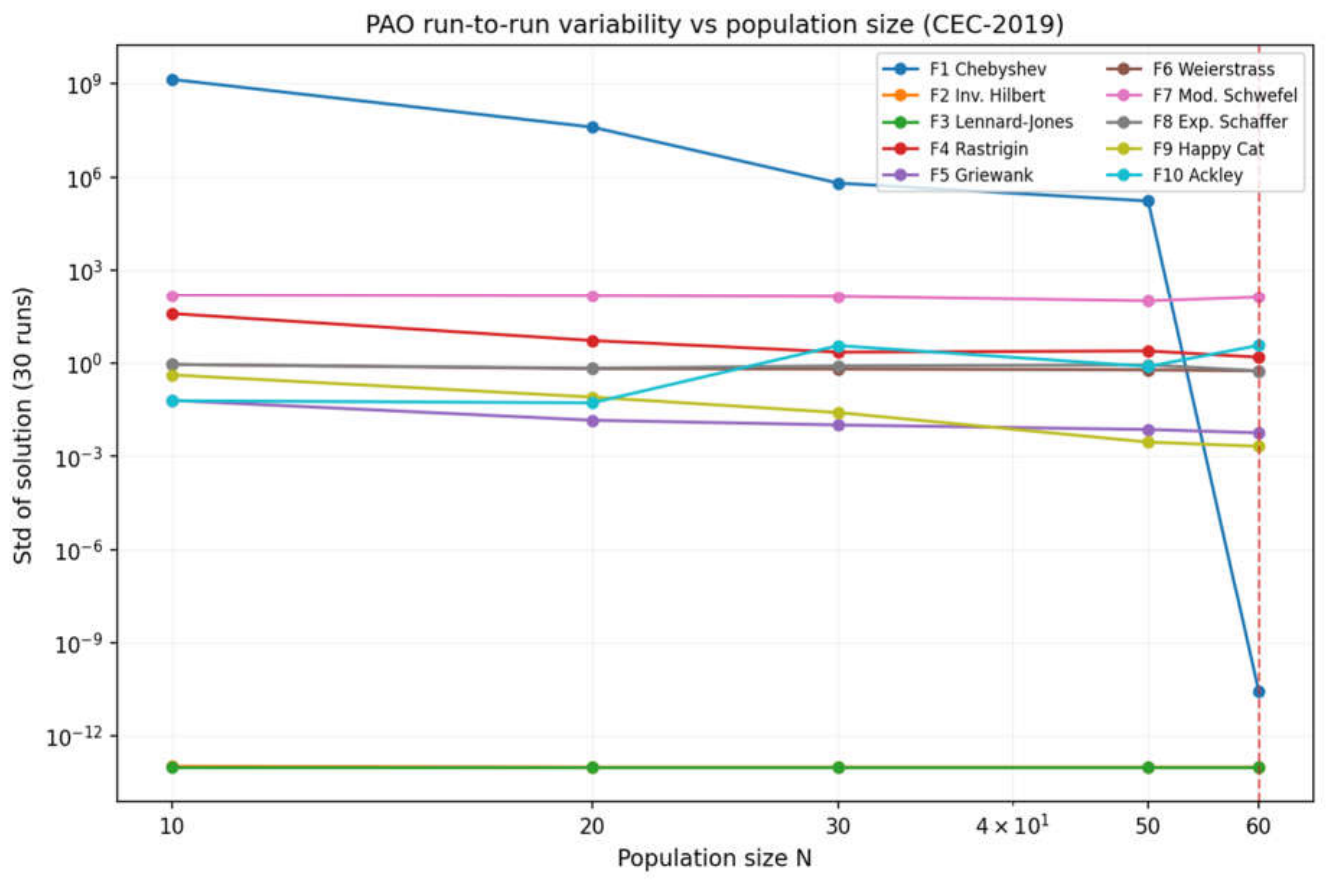
Appendix I. Runtime — Detailed Results
Table I1.
The six fastest algorithms on each suite with their mean runtime, speed rank and accuracy rank. The comparison shows that low computational cost in this pool is not associated with good solution quality: the two fastest methods (HS and DAOA) rank at or near the bottom of the accuracy ordering on every suite.
Table I1.
The six fastest algorithms on each suite with their mean runtime, speed rank and accuracy rank. The comparison shows that low computational cost in this pool is not associated with good solution quality: the two fastest methods (HS and DAOA) rank at or near the bottom of the accuracy ordering on every suite.
| Suite | Algorithm | Mean time / run (s) | Speed rank | Accuracy rank (of 43) |
| Classical-23 | HS | 0.0073 | 1 | 42 |
| Classical-23 | DAOA | 0.0135 | 2 | 43 |
| Classical-23 | CSA | 0.1096 | 3 | 6 |
| Classical-23 | MRSO | 0.1344 | 4 | 31 |
| Classical-23 | TSO | 0.1345 | 5 | 10 |
| Classical-23 | WSO | 0.1437 | 6 | 20 |
| CEC-2017 | HS | 0.0107 | 1 | 36 |
| CEC-2017 | DAOA | 0.0247 | 2 | 43 |
| CEC-2017 | CSA | 0.2176 | 3 | 42 |
| CEC-2017 | SFOA | 0.2380 | 4 | 17 |
| CEC-2017 | MRSO | 0.2437 | 5 | 34 |
| CEC-2017 | SHS | 0.2469 | 6 | 25 |
| CEC-2019 | HS | 0.0244 | 1 | 41 |
| CEC-2019 | DAOA | 0.0845 | 2 | 43 |
| CEC-2019 | MRSO | 0.8923 | 3 | 31 |
| CEC-2019 | SHS | 0.9175 | 4 | 19 |
| CEC-2019 | SFOA | 0.9210 | 5 | 18 |
| CEC-2019 | CSA | 0.9449 | 6 | 42 |
| CEC-2022 | HS | 0.0087 | 1 | 37 |
| CEC-2022 | DAOA | 0.0129 | 2 | 43 |
| CEC-2022 | CSA | 0.0975 | 3 | 42 |
| CEC-2022 | SFOA | 0.1152 | 4 | 6 |
| CEC-2022 | MRSO | 0.1181 | 5 | 30 |
| CEC-2022 | SHS | 0.1219 | 6 | 26 |
Table I2.
PAO mean runtime per run against dimension on the classical suite, showing the near-flat scaling discussed in Section 5.9 and Section 5.11.
Table I2.
PAO mean runtime per run against dimension on the classical suite, showing the near-flat scaling discussed in Section 5.9 and Section 5.11.
| Dimension D | Mean runtime / run (s) | Relative to D = 10 |
| D = 10 | 1.5222 | 1.000× |
| D = 20 | 1.5801 | 1.038× |
| D = 30 | 1.6553 | 1.087× |
| D = 50 | 1.7922 | 1.177× |
| D = 100 | 2.0225 | 1.329× |
Appendix J. Time Complexity — Detailed Results
Supporting detail for Section 5.12. The measured complexity is the dimensionless ratio (T₂ − T₁)/T₀ computed under the standard CEC protocol with T₀ = 0.011449 s, T₁ the objective-only time for the full budget, and T₂ the mean complete-algorithm time over five runs on each of the 23 classical functions.
Table J1.
Complete time-complexity ranking of all 43 algorithms. “Mean rank per function” is the average of the per-function complexity ranks and is shown because it is less sensitive to a single expensive function than the mean ratio. The final three algorithms produced no valid measurement on any function and cannot be ranked.
Table J1.
Complete time-complexity ranking of all 43 algorithms. “Mean rank per function” is the average of the per-function complexity ranks and is shown because it is less sensitive to a single expensive function than the mean ratio. The final three algorithms produced no valid measurement on any function and cannot be ranked.
| # | Algorithm | Mean measured complexity | Mean rank per function | Valid functions (of 23) |
| 1 | CSA | 1.55 | 1 | 7 |
| 2 | SHS | 9.58 | 3.53 | 17 |
| 3 | MRSO | 9.71 | 3.44 | 18 |
| 4 | TSO | 10.37 | 4.37 | 19 |
| 5 | WSO | 14.67 | 6.18 | 22 |
| 6 | PSO | 15.95 | 6.5 | 22 |
| 7 | AOA | 16.24 | 4.73 | 22 |
| 8 | SFOA | 16.51 | 6.94 | 16 |
| 9 | FOA | 17.31 | 6.57 | 23 |
| 10 | SO | 29.4 | 8.65 | 23 |
| 11 | YDSE | 30.3 | 10.09 | 23 |
| 12 | GWO | 33.76 | 8.64 | 22 |
| 13 | FOX | 35.96 | 11.52 | 23 |
| 14 | DSWO | 40.7 | 12.52 | 23 |
| 15 | GOOSE | 45.94 | 14.22 | 23 |
| 16 | DHOLE | 48.21 | 11.35 | 23 |
| 17 | CS | 56.96 | 15.78 | 23 |
| 18 | HBA | 67.9 | 17.61 | 23 |
| 19 | ZOA | 85.94 | 15.87 | 23 |
| 20 | FPA | 100.69 | 20.3 | 23 |
| 21 | SOA | 109.95 | 19.7 | 23 |
| 22 | DRA | 119.38 | 23.52 | 23 |
| 23 | RFO | 122.09 | 23.13 | 23 |
| 24 | WUTP | 129.85 | 19.57 | 23 |
| 25 | AO | 140.55 | 22.7 | 23 |
| 26 | EHO | 153.27 | 21.48 | 23 |
| 27 | GOA | 164.76 | 23.96 | 23 |
| 28 | NDO | 196.87 | 26.57 | 23 |
| 29 | SPIBA | 213.35 | 28.09 | 23 |
| 30 | MSO | 244.15 | 27.13 | 23 |
| 31 | DE | 287.2 | 30.52 | 23 |
| 32 | PGA | 417.4 | 32.09 | 23 |
| 33 | APO | 492.64 | 33.52 | 23 |
| 34 | PAO | 511.68 | 34.17 | 23 |
| 35 | CPO | 515.79 | 34.65 | 23 |
| 36 | WAA | 646.84 | 31.39 | 23 |
| 37 | SHO | 805.42 | 32.43 | 23 |
| 38 | Chimp | 942.13 | 32.78 | 23 |
| 39 | MRA | 1111.8 | 33.91 | 23 |
| 40 | EMRA | 1261.98 | 34.87 | 23 |
| -- | HS | -- | -- | 0 |
| -- | DAOA | -- | -- | 0 |
| -- | DOA | -- | -- | 0 |
Table J2.
PAO per-function measured complexity on the 23 classical benchmark functions, with PAO’s complexity rank on each function and the lightest measured complexity recorded on that function for reference. The narrow range (415.8–613.4) confirms that PAO’s overhead is stable across problem types.
Table J2.
PAO per-function measured complexity on the 23 classical benchmark functions, with PAO’s complexity rank on each function and the lightest measured complexity recorded on that function for reference. The narrow range (415.8–613.4) confirms that PAO’s overhead is stable across problem types.
| Function | PAO measured complexity | PAO complexity rank | Lightest on this function |
| F1 | 481.3 | 34 | 6.1 |
| F2 | 546.1 | 34 | 1.1 |
| F3 | 474.0 | 28 | 3.5 |
| F4 | 494.6 | 34 | 0.8 |
| F5 | 542.6 | 33 | 8.7 |
| F6 | 613.4 | 34 | 10.2 |
| F7 | 515.0 | 28 | 3.6 |
| F8 | 590.8 | 33 | 2.0 |
| F9 | 572.8 | 33 | 2.5 |
| F10 | 588.5 | 30 | 4.7 |
| F11 | 540.3 | 31 | 2.1 |
| F12 | 574.8 | 26 | 3.1 |
| F13 | 584.9 | 29 | 5.5 |
| F14 | 542.5 | 33 | 2.9 |
| F15 | 475.0 | 38 | 6.4 |
| F16 | 441.1 | 39 | 1.6 |
| F17 | 462.0 | 39 | 0.5 |
| F18 | 415.8 | 39 | 0.5 |
| F19 | 461.9 | 38 | 3.2 |
| F20 | 418.5 | 39 | 0.2 |
| F21 | 474.5 | 38 | 5.7 |
| F22 | 477.8 | 38 | 7.4 |
| F23 | 480.3 | 38 | 0.3 |
Note. Three algorithms (HS, DAOA and DOA) are omitted from the ranking because on every function either all timing runs failed or the complete-algorithm time fell below the objective-only time, indicating that the full evaluation budget was not consumed; the resulting ratio would be negative. A further group — CSA (valid on 7 functions), SFOA (16), SHS (17), MRSO (18) and TSO (19) — is ranked on partial measurements only, and their positions near the top of the ranking should be read with that in mind. PAO, together with 30 other algorithms, was measured successfully on all 23 functions.
Appendix K. Ablation Study — Detailed Results
Per-function results underlying Section 5.13. All values are mean solution error f(x) − f* over 30 runs on the CEC-2017 suite (29 functions; F2 omitted per the standard convention), reported in scientific E-notation.
Table K1.
Mean solution error for the full algorithm and each ablated variant on every CEC-2017 function. The no-Fajr column reproduces the full algorithm exactly on all functions except F20.
Table K1.
Mean solution error for the full algorithm and each ablated variant on every CEC-2017 function. The no-Fajr column reproduces the full algorithm exactly on all functions except F20.
| Fn | Full PAO | no-Fajr | no-Dhuhr | no-Asr | no-Maghrib | no-Isha | BaseEngineOnly | FixedSchedule | RandomSchedule |
| F1 | 1.058 × 10² | 1.058 × 10² | 8.490 × 10¹ | 1.318 × 10² | 1.004 × 10² | 9.142 × 10¹ | 2.312 × 10⁰ | 1.732 × 10³ | 8.885 × 10⁰ |
| F3 | 1.441 × 10³ | 1.441 × 10³ | 1.551 × 10³ | 1.832 × 10³ | 1.386 × 10³ | 1.360 × 10³ | 7.289 × 10³ | 3.596 × 10³ | 1.339 × 10² |
| F4 | 8.834 × 10¹ | 8.834 × 10¹ | 8.828 × 10¹ | 8.890 × 10¹ | 8.759 × 10¹ | 8.858 × 10¹ | 7.856 × 10¹ | 9.022 × 10¹ | 6.947 × 10¹ |
| F5 | 8.278 × 10¹ | 8.278 × 10¹ | 7.675 × 10¹ | 8.836 × 10¹ | 8.482 × 10¹ | 8.467 × 10¹ | 7.465 × 10¹ | 1.056 × 10¹ | 4.448 × 10¹ |
| F6 | 7.294 × 10⁻³ | 7.294 × 10⁻³ | 1.158 × 10⁻² | 9.847 × 10⁻³ | 6.873 × 10⁻³ | 7.174 × 10⁻³ | 9.134 × 10⁻⁴ | 1.287 × 10⁻¹ | 4.546 × 10⁻² |
| F7 | 1.247 × 10² | 1.247 × 10² | 1.089 × 10² | 1.268 × 10² | 1.230 × 10² | 1.237 × 10² | 1.074 × 10² | 4.491 × 10¹ | 8.756 × 10¹ |
| F8 | 8.777 × 10¹ | 8.777 × 10¹ | 7.812 × 10¹ | 9.250 × 10¹ | 8.691 × 10¹ | 8.797 × 10¹ | 7.801 × 10¹ | 1.208 × 10¹ | 4.516 × 10¹ |
| F9 | 8.103 × 10⁻² | 8.103 × 10⁻² | 4.112 × 10⁻¹ | 7.805 × 10⁻² | 8.103 × 10⁻² | 8.103 × 10⁻² | 5.104 × 10⁻¹ | 4.787 × 10⁰ | 8.615 × 10⁰ |
| F10 | 5.291 × 10³ | 5.291 × 10³ | 4.328 × 10³ | 5.233 × 10³ | 5.290 × 10³ | 5.261 × 10³ | 4.269 × 10³ | 4.061 × 10³ | 5.862 × 10³ |
| F11 | 5.194 × 10¹ | 5.194 × 10¹ | 5.883 × 10¹ | 5.358 × 10¹ | 5.303 × 10¹ | 5.204 × 10¹ | 6.645 × 10¹ | 5.069 × 10¹ | 8.805 × 10¹ |
| F12 | 2.565 × 10⁴ | 2.565 × 10⁴ | 2.436 × 10⁴ | 2.560 × 10⁴ | 2.455 × 10⁴ | 2.551 × 10⁴ | 1.744 × 10⁴ | 2.874 × 10⁴ | 1.642 × 10⁴ |
| F13 | 3.842 × 10² | 3.842 × 10² | 3.082 × 10² | 3.453 × 10² | 3.919 × 10² | 3.854 × 10² | 2.170 × 10² | 4.740 × 10² | 2.067 × 10² |
| F14 | 4.664 × 10¹ | 4.664 × 10¹ | 5.093 × 10¹ | 4.657 × 10¹ | 4.677 × 10¹ | 4.673 × 10¹ | 5.397 × 10¹ | 6.493 × 10¹ | 8.617 × 10¹ |
| F15 | 8.876 × 10¹ | 8.876 × 10¹ | 9.730 × 10¹ | 8.671 × 10¹ | 9.039 × 10¹ | 8.941 × 10¹ | 9.463 × 10¹ | 1.720 × 10² | 1.417 × 10² |
| F16 | 6.673 × 10² | 6.673 × 10² | 8.022 × 10² | 6.476 × 10² | 6.708 × 10² | 6.639 × 10² | 9.238 × 10² | 1.720 × 10² | 5.228 × 10² |
| F17 | 1.603 × 10² | 1.603 × 10² | 2.354 × 10² | 1.691 × 10² | 1.573 × 10² | 1.618 × 10² | 3.229 × 10² | 5.019 × 10¹ | 1.207 × 10² |
| F18 | 1.709 × 10² | 1.709 × 10² | 1.683 × 10² | 2.049 × 10² | 1.691 × 10² | 1.770 × 10² | 8.815 × 10³ | 7.258 × 10² | 1.796 × 10² |
| F19 | 4.919 × 10¹ | 4.919 × 10¹ | 4.678 × 10¹ | 4.915 × 10¹ | 4.924 × 10¹ | 4.910 × 10¹ | 5.128 × 10¹ | 6.750 × 10¹ | 8.631 × 10¹ |
| F20 | 1.914 × 10² | 1.895 × 10² | 3.101 × 10² | 1.834 × 10² | 1.924 × 10² | 1.887 × 10² | 3.664 × 10² | 9.907 × 10¹ | 1.870 × 10² |
| F21 | 2.768 × 10² | 2.768 × 10² | 2.771 × 10² | 2.774 × 10² | 2.780 × 10² | 2.775 × 10² | 2.749 × 10² | 2.125 × 10² | 2.294 × 10² |
| F22 | 2.840 × 10² | 2.840 × 10² | 5.309 × 10² | 2.599 × 10² | 2.889 × 10² | 2.892 × 10² | 5.226 × 10² | 2.387 × 10² | 1.003 × 10² |
| F23 | 4.297 × 10² | 4.297 × 10² | 4.294 × 10² | 4.347 × 10² | 4.298 × 10² | 4.313 × 10² | 4.286 × 10² | 3.702 × 10² | 3.878 × 10² |
| F24 | 4.931 × 10² | 4.931 × 10² | 4.968 × 10² | 4.834 × 10² | 4.993 × 10² | 4.950 × 10² | 4.948 × 10² | 4.421 × 10² | 4.457 × 10² |
| F25 | 3.872 × 10² | 3.872 × 10² | 3.872 × 10² | 3.872 × 10² | 3.872 × 10² | 3.872 × 10² | 3.873 × 10² | 3.878 × 10² | 3.872 × 10² |
| F26 | 1.681 × 10³ | 1.681 × 10³ | 1.760 × 10³ | 1.663 × 10³ | 1.720 × 10³ | 1.655 × 10³ | 1.735 × 10³ | 1.287 × 10³ | 1.354 × 10³ |
| F27 | 5.028 × 10² | 5.028 × 10² | 5.056 × 10² | 5.030 × 10² | 5.028 × 10² | 5.028 × 10² | 5.042 × 10² | 5.097 × 10² | 5.113 × 10² |
| F28 | 4.071 × 10² | 4.071 × 10² | 4.044 × 10² | 4.075 × 10² | 4.033 × 10² | 4.081 × 10² | 4.009 × 10² | 4.262 × 10² | 3.854 × 10² |
| F29 | 6.409 × 10² | 6.409 × 10² | 6.644 × 10² | 6.473 × 10² | 6.410 × 10² | 6.395 × 10² | 6.672 × 10² | 5.301 × 10² | 5.635 × 10² |
| F30 | 2.533 × 10³ | 2.533 × 10³ | 2.529 × 10³ | 2.526 × 10³ | 2.542 × 10³ | 2.548 × 10³ | 2.381 × 10³ | 2.700 × 10³ | 2.581 × 10³ |
Table K2.
The five functions on which each schedule ablation degrades most severely, expressed as the percentage increase in mean error relative to the full algorithm. These tail failures are what the astronomical schedule prevents and are the reason the full configuration is retained despite its neutral median behaviour.
Table K2.
The five functions on which each schedule ablation degrades most severely, expressed as the percentage increase in mean error relative to the full algorithm. These tail failures are what the astronomical schedule prevents and are the reason the full configuration is retained despite its neutral median behaviour.
| Variant | Function | Increase in mean error (%) |
| BaseEngineOnly | F18 | +5059 |
| BaseEngineOnly | F9 | +530 |
| BaseEngineOnly | F3 | +406 |
| BaseEngineOnly | F17 | +101 |
| BaseEngineOnly | F20 | +91 |
| FixedSchedule | F9 | +5807 |
| FixedSchedule | F6 | +1664 |
| FixedSchedule | F1 | +1537 |
| FixedSchedule | F18 | +325 |
| FixedSchedule | F3 | +149 |
| RandomSchedule | F9 | +10531 |
| RandomSchedule | F6 | +523 |
| RandomSchedule | F14 | +85 |
| RandomSchedule | F19 | +75 |
| RandomSchedule | F11 | +70 |
Figure K.1.
Average rank of the nine configurations across the 29 CEC-2017 functions (lower is better). The nine
configurations span a narrow band from 4.00 to 5.28, confirming that no single ablation changes the algorithm’s
standing dramatically on the averaged-rank metric.
Figure K.1.
Average rank of the nine configurations across the 29 CEC-2017 functions (lower is better). The nine
configurations span a narrow band from 4.00 to 5.28, confirming that no single ablation changes the algorithm’s
standing dramatically on the averaged-rank metric.
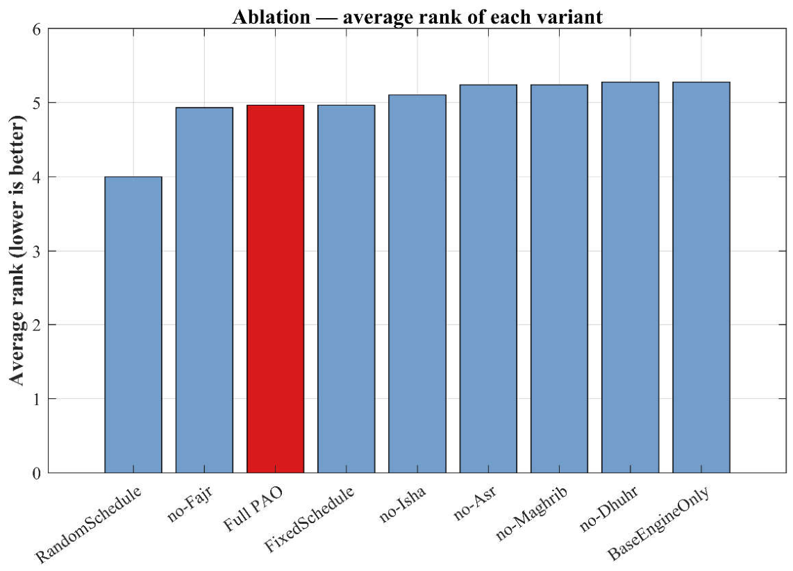
Appendix L. Real-World Engineering Problems — Detailed Results
L.1 Scope, Protocol and how to Read this Appendix
Supporting detail for Section 6. All results are over 30 independent runs of 500 iterations with a population of N = 60 on the twenty-two constrained design problems, with constraints handled by the shared static-penalty wrapper of Section 6.1.
This appendix serves two purposes that were previously separated. Section L.2 documents each of the twenty-two applications individually — its engineering goal, design variables, objective function, constraints and reference optimum, with a labelled diagram where the geometry is defined by a small number of dimensions. Section L.3 then reports the aggregate results across the whole suite, so that a reader can move from what each problem is to how the algorithms perform on it without leaving the appendix. Section L.4 lists the per-problem material held in the result archive rather than in the document.
All formulations are reproduced exactly as implemented in the code, so that every number reported in Section 6 can be traced to a specific objective and constraint set.
Constraint handling. Every application is an inequality-constrained minimization of the form subject to . Constraints are enforced by the static penalty method of the reference implementation,
A note on the reference optima. For P14, P17, P18, P20 and P21 the best-known values reported in the literature differ between sources. They are used here as comparison targets, not as verified global optima, and Section 6.5 discusses the consequences.
L.2 The Twenty-Two Applications
Each entry below states the engineering goal, the design variables with their physical meaning and bounds, the objective function, the constraint set, and the best-known objective value used as the reference optimum. The formulations are reproduced exactly as implemented in the code, so every number in Section 6 and in Section L.3 can be traced to a specific objective and constraint set. The applications are grouped by engineering domain; the identifiers PNN match the problem numbering used throughout Section 6 and in Tables L1–L3.
L.2.1 Structural Design Problems
P04: Three-bar truss
| Goal: | Minimize the volume (hence material cost) of a symmetric two-dimensional truss of three bars carrying a single vertical load, subject to stress limits in every member (see Figure L1). |
| Variables: | (). = cross-sectional area of the two inclined bars; = area of the vertical bar. Both are normalized areas in [0, 1]. |
| Objective: |
the total bar volume for a unit member length of 100 cm. |
| Constraints (3). | Stress limits at the loaded joint, each written so that the axial stress in a member does not exceed the allowable value; the third constraint governs the vertical bar under reversed loading. |
| Reference optimum: | 263.895843 |
| Source: | (Talatahari, Bayzidi, et al., 2021) |
Figure L1.
Three-bar truss: two inclined bars of area x₁ and one vertical bar of area x₂, pinned to a rigid support and loaded at the lower joint.
Figure L1.
Three-bar truss: two inclined bars of area x₁ and one vertical bar of area x₂, pinned to a rigid support and loaded at the lower joint.
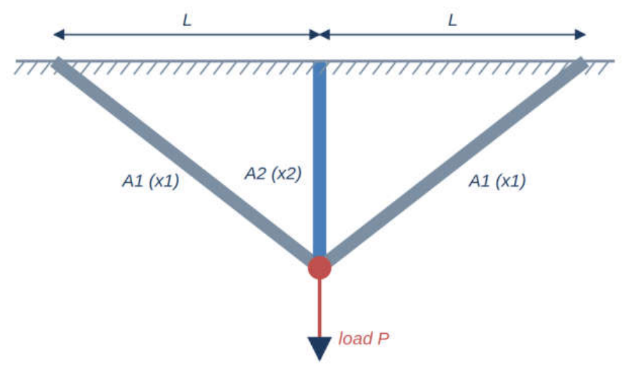
P06 — Cantilever beam
| Goal: | Minimize the weight of a stepped cantilever beam built from five hollow square elements of equal length, subject to a limit on tip deflection (see Figure L2). |
| Variables: | (). the cross-sectional height of the five successive elements, each in [0.01, 100]. |
| Objective: |
|
| Constraints (1). | A single deflection constraint, |
| Reference optimum: | 1.3399576 |
| Source: | (Abdulla et al., 2024) |
Figure L2.
Stepped cantilever beam: five elements of decreasing section, fixed at the left and loaded at the free end.
Figure L2.
Stepped cantilever beam: five elements of decreasing section, fixed at the left and loaded at the free end.
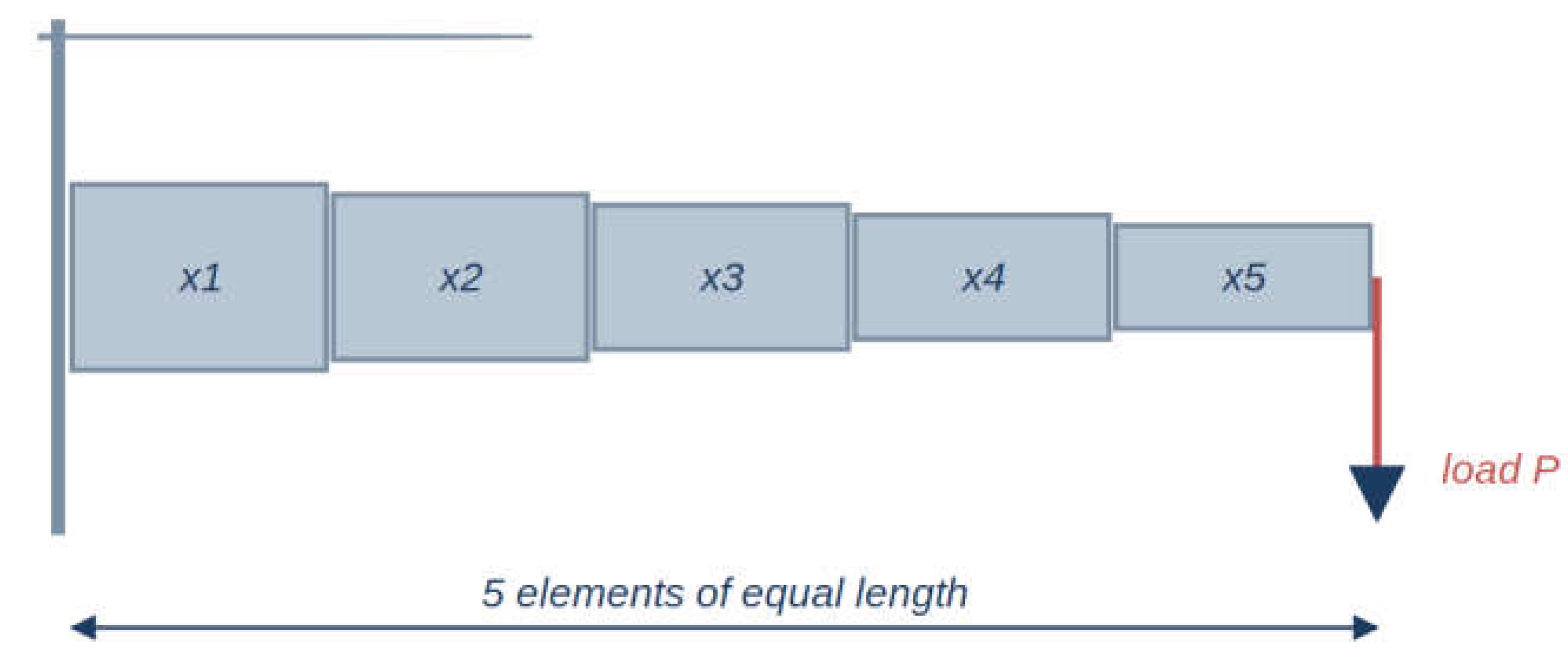
P07 — I-beam vertical deflection
| Goal: | Minimize the vertical deflection of a simply supported I-section beam under a central load, which is equivalent to maximizing its bending stiffness for a bounded cross-section (see Figure L3). |
| Variables: | (). x₁ = section height h ∈ [10,80]; x₂ = flange width b ∈ [10,50]; x₃ = web thickness = flange thickness all in cm. |
| Objective: |
where I is the second moment of area assembled from the web and the two flanges. |
| Constraints (2). | An upper limit on the cross-sectional area ) and a combined bending-stress constraint. |
| Reference optimum: | 1. 0130741 |
| Source: | (Houssein et al., 2025) |
Figure L3.
I-beam cross-section: overall height h, flange width b, web thickness and flange thickness .
Figure L3.
I-beam cross-section: overall height h, flange width b, web thickness and flange thickness .
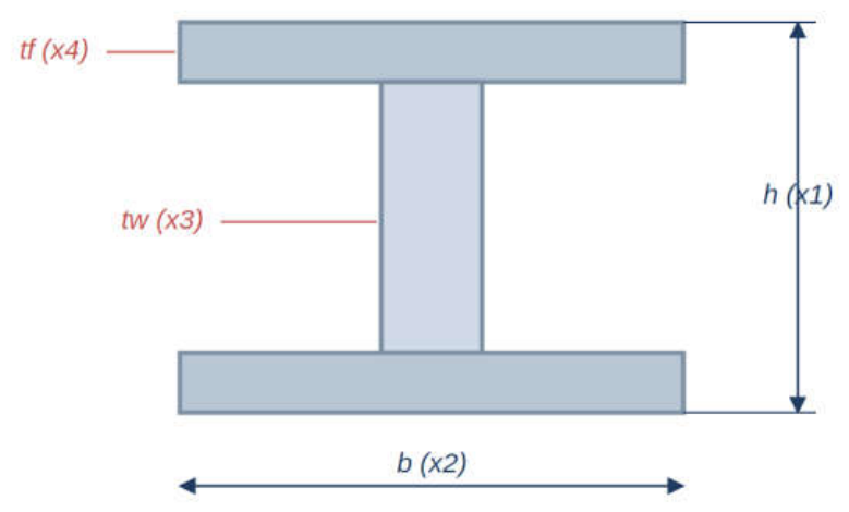
P08 — Tubular column
| Goal: | Minimize the cost of a hollow circular column carrying an axial compressive load, subject to yield and buckling limits (see Figure L4). |
| Variables: | (). x₁ = mean diameter d ∈ [2,14] cm; x₂ = wall thickness t ∈ [0.2, 0.8] cm |
| Objective: |
combining material and construction cost |
| Constraints (6). | Induced-stress limit, Euler buckling limit, and four geometric bounds on the diameter and the diameter-to-thickness ratio. |
| Reference optimum: | 26.486361473 |
| Source: | (Houssein et al., 2025) |
Figure L4.
Tubular column of mean diameter and wall thickness under an axial load.
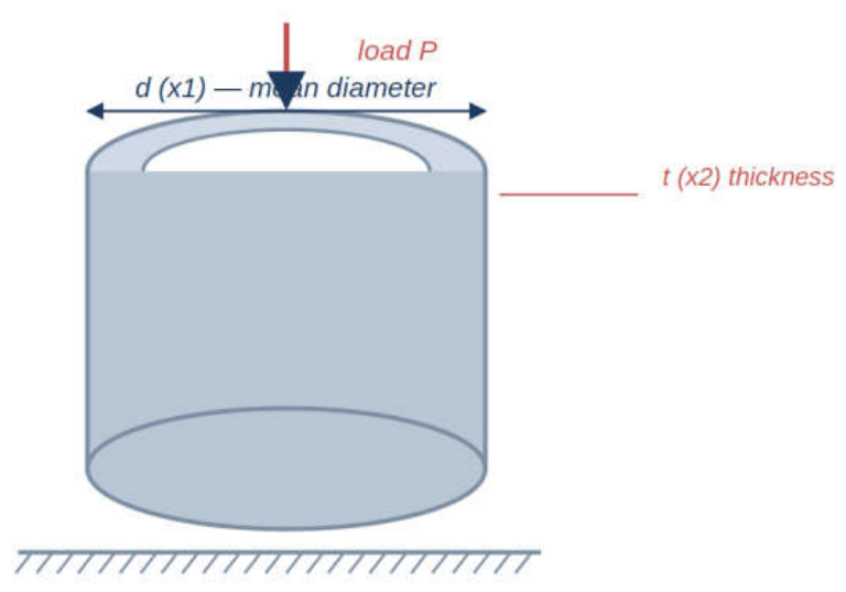
P12 — Welded beam
| Goal: | Minimize the fabrication cost of a beam welded to a rigid support and carrying a load at its free end, subject to limits on weld and beam stresses, deflection and buckling (see Figure L5). |
| Variables: | (). = weld thickness h ∈ [0.1, 2]; x₂ = weld/attachment length L ∈ [0.1, 10]; x₃ = beam depth t ∈ [0.1, 10]; x₄ = beam thickness b ∈ [0.1, 2], all in inches. |
| Objective: |
|
| Constraints (7). | Shear stress in the weld (), bending stress in the beam (), the geometric conditiona cost side-constraint, a minimum weld thickness, tip deflection (in) and the bar buckling load (). |
| Reference optimum: | 26.486361473 |
| Source: | (Houssein et al., 2025) |
Figure L5.
Welded beam: fillet welds of thickness and length L attach a bar of depth t and thickness b to a rigid support.
Figure L5.
Welded beam: fillet welds of thickness and length L attach a bar of depth t and thickness b to a rigid support.
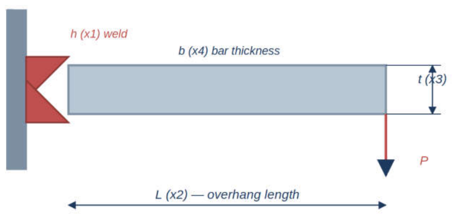
P13 — Reinforced concrete beam
| Goal: | Minimize the combined cost of steel reinforcement and concrete in a singly reinforced beam of rectangular section, subject to a flexural-strength requirement and a proportion limit (see Figure L6). |
| Variables: | (). of reinforcing steel As, selected from a discrete catalogue of eleven standard bar areas; x₂ = beam width b, selected from the integer set 28…40 cm; x₃ = beam depth h ∈ [5,10] cm. The two discrete variables are resolved inside the objective, so any continuous optimizer can be used. |
| Objective: |
|
| Constraints (2). | The depth-to-width ratio and a flexural-capacity requirement relating to |
| Reference optimum: | 359.2080 |
| Source: | (Kaveh & Sabzi, 2011) |
Figure L6.
Reinforced concrete beam section: width b, depth h and tensile steel area .
P22 — Ten-bar planar truss
| Goal: | Minimize the weight of the classical ten-bar cantilever truss, subject to stress limits in all ten members and displacement limits at all free nodes. This is the largest structural problem in the suite and the only one solved by an embedded finite-element analysis (see Figure L7). |
| Variables: | (). |
| Objective: |
|
| Constraints (18). | Ten stress constraints (|σᵢ| ≤ 25 000 psi) and eight nodal-displacement constraints (|u| ≤ 2 in).. |
| Reference optimum: | 5060.85 lb |
| Source: | (Ghaemifard & Ghannadiasl, 2024) |
Figure L7.
Ten-bar planar truss: six nodes, ten members, two 100-kip loads applied at the lower free nodes, with nodes 5 and 6 fixed.
Figure L7.
Ten-bar planar truss: six nodes, ten members, two 100-kip loads applied at the lower free nodes, with nodes 5 and 6 fixed.
L.2.2 Mechanical Design Problems
P01 — Speed reducer (gearbox)
| Goal: | Goal. Minimize the weight of a single-stage speed reducer, subject to limits on gear-tooth bending and surface stress, shaft deflection, and shaft stress. It is the highest-dimensional of the classical mechanical problems and the most heavily constrained (see Figure L8). |
| Variables: | (). |
| Objective: | A weight expression combining the gear body, the two shafts and the bearings |
| Constraints (11). | Bending and contact stress in the gear teeth, transverse deflection of both shafts, stresses in both shafts, and geometric conditions on the face-width-to-module ratio and the shaft dimensions. |
| Reference optimum: | 2994.4244658 |
| Source: | (Abdulla et al., 2024) |
Figure L8.
Speed reducer: gear pair of module m and z teeth on a face of width , carried on two shafts of lengths and diameters .
Figure L8.
Speed reducer: gear pair of module m and z teeth on a face of width , carried on two shafts of lengths and diameters .
P02 — Tension/compression spring
| Goal: | Minimize the mass of a helical spring subject to limits on shear stress, surge frequency and minimum deflection (see Figure L9). |
| Variables: | (). x₁ = wire diameter d ∈ [0.05, 2]; x₂ = mean coil diameter D ∈ [0.25, 1.3]; x₃ = number of active coils N ∈ [2,15]. |
| Objective: |
|
| Constraints (4). | Minimum deflection, shear stress, surge frequency, and a limit on the outside diameter. |
| Reference optimum: | 012665232788 |
| Source: | (Abdulla et al., 2024) |
Figure L9.
Helical tension/compression spring: wire diameter , mean coil diameter , and active coils.
Figure L9.
Helical tension/compression spring: wire diameter , mean coil diameter , and active coils.
P05 — Gear train
| Goal: | Choose four integer tooth counts so that the resulting gear ratio matches the required value ofas closely as possible. The problem is unconstrained but purely discrete, and its objective is extremely flat near the optimum (see Figure L10). |
| Variables: | (). tooth counts of the four gears, each an integer in [12,60]; the values are rounded inside the objective. |
| Objective: |
|
| Constraints | None beyond the variable bounds |
| Reference optimum: | 2.700857 × 10⁻¹² |
| Source: | (Hasan & Aladdin, 2025) |
Figure L10.
Gear train: four gears whose tooth counts determine the transmitted ratio.
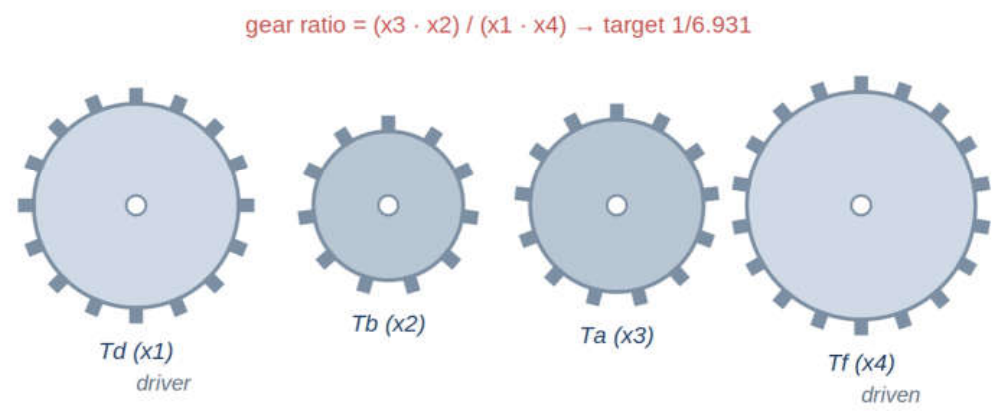
P03 — Pressure vessel
| Goal: | Minimize the total cost of a cylindrical pressure vessel with hemispherical heads, covering material, forming and welding, subject to code requirements on wall thickness and volume (see Figure L11). |
| Variables: | (). = shell thickness and = head thickness both discrete multiples of 0.0625 in, resolved by rounding inside the objective; = inner radius of the cylindrical section |
| Objective: | |
| Constraints (4) | Two minimum-thickness requirements (), a minimum volume requirement () and a limit on the cylindrical length (). |
| Reference optimum: | 6059.714335 |
| Source: | (Hasan & Aladdin, 2025) |
Figure L11.
Pressure vessel: cylindrical body of inner radius and length closed by hemispherical heads, with shell and head thicknesses and .
Figure L11.
Pressure vessel: cylindrical body of inner radius and length closed by hemispherical heads, with shell and head thicknesses and .
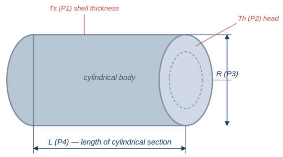
P14 — Multiple-disk clutch brake
| Goal: | Minimize the mass of a multiple-disk clutch brake, subject to limits on contact pressure, sliding velocity, actuating force, torque capacity and stopping time (see Figure L12). |
| Variables: | (). (integer, rounded inside the objective). |
| Objective: |
|
| Constraints (8) | Minimum radius difference, axial length, contact pressure, the pressure–velocity product, sliding velocity, stopping time, torque capacity, and a non-negativity condition on the stopping time. |
| Reference optimum: | 0.235242 |
| Source: | (Dhiman, 2021) |
Figure L12.
Multiple-disk clutch brake: annular friction discs of inner radius and outer radius .
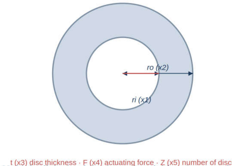
P16 — Belleville disc spring
| Goal: | Minimize the mass of a conical disc (Belleville) spring subject to limits on compressive stress, deflection, spring height and geometric proportion (see Figure L13). |
| Variables: | (). |
| Objective: |
the disc mass. |
| Constraints (7) | Compressive stress limit, deflection–load relationship, the height-to-thickness condition, overall height limit, maximum outer diameter, the requirement and a slope limit |
| Reference optimum: | 1.979675 |
| Source: | (Kumar et al., 2020) |
Figure L13.
Belleville disc spring: outer diameter , inner diameter , thickness and free height.
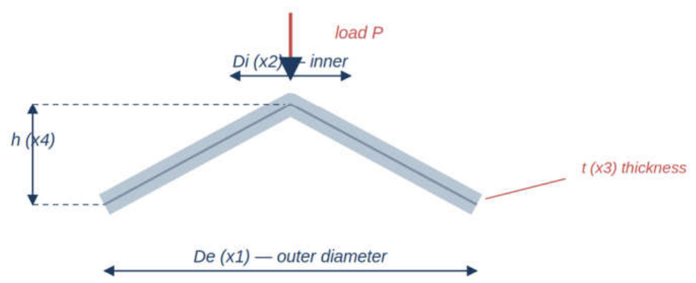
P09 — Piston lever
| Goal: | Position the pivot of a hydraulic piston lever so that the oil volume required to raise the lever through a specified angle is minimized, subject to force, moment and geometric constraints (see Figure L14). |
| Variables: | (). |
| Objective: |
|
| Constraints (4) | Moment equilibrium under the applied load, a maximum-moment limit, a stroke condition on the piston lengths, and the geometric condition |
| Reference optimum: | 8.41269832311 |
| Source: | (Kumar et al., 2020) |
Figure L14.
Piston lever. Pivot at the fixed support, hydraulic cylinder of piston diameter D, and the lever geometry that positions the pivot; the objective is the swept oil volume required to raise the lever through 45°.
Figure L14.
Piston lever. Pivot at the fixed support, hydraulic cylinder of piston diameter D, and the lever geometry that positions the pivot; the objective is the swept oil volume required to raise the lever through 45°.
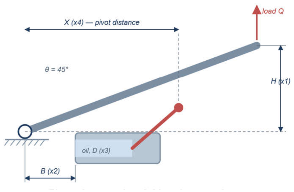
P15 — Rolling element bearing
| Goal: | Maximize the dynamic load-carrying capacity of a rolling-element bearing. Because the framework minimizes, the problem is exposed as minimization of the negative capacity, so its objective values are negative (see Figure L15). |
| Variables: | (). Pitch diameter ball diameter number of balls (integer), inner and outer raceway groove curvature coefficients and five design parameters that constrain the internal geometry |
| Objective: |
where is the dynamic capacity is computed from the standard bearing-life formula, with different expressions for ball diameters below and above 25.4 mm. |
| Constraints (9) | Assembly-angle feasibility bounds on the ball diameter relative to the bore, a width condition, bounds on the pitch diameter, a groove-clearance condition, and two curvature limits |
| Reference optimum: | −85,539, 85,539 |
| Source: | (Kumar et al., 2020) |
Figure L15.
Rolling element bearing. Radial section showing the bore d, Z balls of diameter on the pitch circle , and the raceway groove curvatures and . The dynamic capacity is maximised, so the objective is reported as −.
Figure L15.
Rolling element bearing. Radial section showing the bore d, Z balls of diameter on the pitch circle , and the raceway groove curvatures and . The dynamic capacity is maximised, so the objective is reported as −.
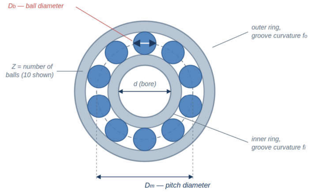
P17 — Hydrostatic thrust bearing
| Goal: | Minimize the total power loss of hydrostatic thrust bearing, comprising pumping power and friction power, subject to load capacity, pressure, temperature-rise, film-thickness and stress limits (see Figure L16). |
| Variables: | (). |
| Objective: |
|
| Constraints (7) | Minimum load capacity, maximum inlet pressure, maximum oil-temperature rise, minimum film thickness, the geometric condition an inlet-velocity condition and a maximum bearing pressure |
| Reference optimum: | 1625.44 (values from 1610 to 1640 are reported). |
| Source: | (Kumar et al., 2020) |
Figure L16.
Hydrostatic thrust bearing. Circular pad of radius with a central recess of radius , fed with oil of viscosity at flow rate , supporting a rotating shaft under load ; the objective is the sum of pumping and friction power loss.
Figure L16.
Hydrostatic thrust bearing. Circular pad of radius with a central recess of radius , fed with oil of viscosity at flow rate , supporting a rotating shaft under load ; the objective is the sum of pumping and friction power loss.
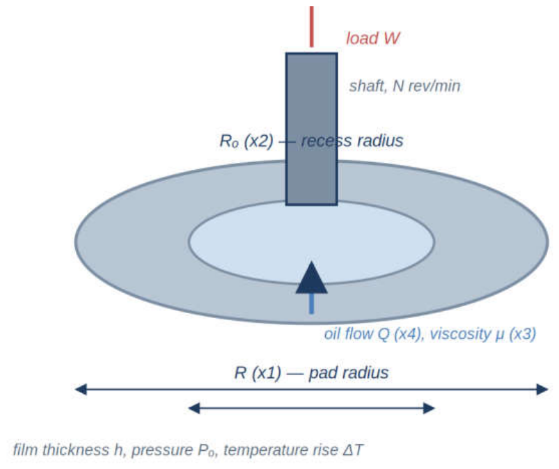
P18 — Robot gripper
| Goal: | Minimize the difference between the maximum and minimum gripping force generated over the full displacement range of a four-bar robot gripper mechanism, so that the grip force is as uniform as possible (see Figure L17). |
| Variables: | (). Link lengths the offset e, the dimension f, the actuator strokeand the angle rad. |
| Objective: |
|
| Constraints (7) | Bounds on the gripper opening at the two extremes of travel, and four geometric conditions ensuring the linkage assembles and does not lock. |
| Reference optimum: | 2.5287 (values from 2.5 to 4.2 are reported) |
| Source: | (Kumar et al., 2020) |
Figure L17.
Robot gripper. Four-bar linkage driven by an actuator through displacement z, with link lengths offset e and angle ; the objective is the difference between the maximum and minimum gripping force over the full range of travel.
Figure L17.
Robot gripper. Four-bar linkage driven by an actuator through displacement z, with link lengths offset e and angle ; the objective is the difference between the maximum and minimum gripping force over the full range of travel.
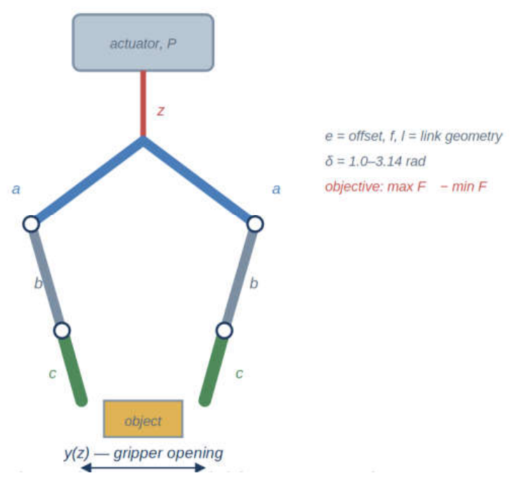
P20 — Stepped cone pulley
| Goal: | Minimize the mass of a four-step cone pulley that must transmit a specified power at four different speeds, subject to equal-belt-length, tension-ratio and power constraints (see Figure L18). |
| Variables: | (). the diameters of the four steps |
| Objective: |
|
| Constraints (11) | Three equal-belt-length conditions (equality constraints encoded as four tension-ratio conditions () and four transmitted-power conditions. |
| Reference optimum: | 16.63 (approximate) |
| Source: | (Kumar et al., 2020) |
Figure L18.
Stepped cone pulley. Four steps of diameters on a common shaft of width , driven by one belt at four output speeds; the objective is total pulley mass subject to equal belt length, tension ratio and transmitted power.
Figure L18.
Stepped cone pulley. Four steps of diameters on a common shaft of width , driven by one belt at four output speeds; the objective is total pulley mass subject to equal belt length, tension ratio and transmitted power.
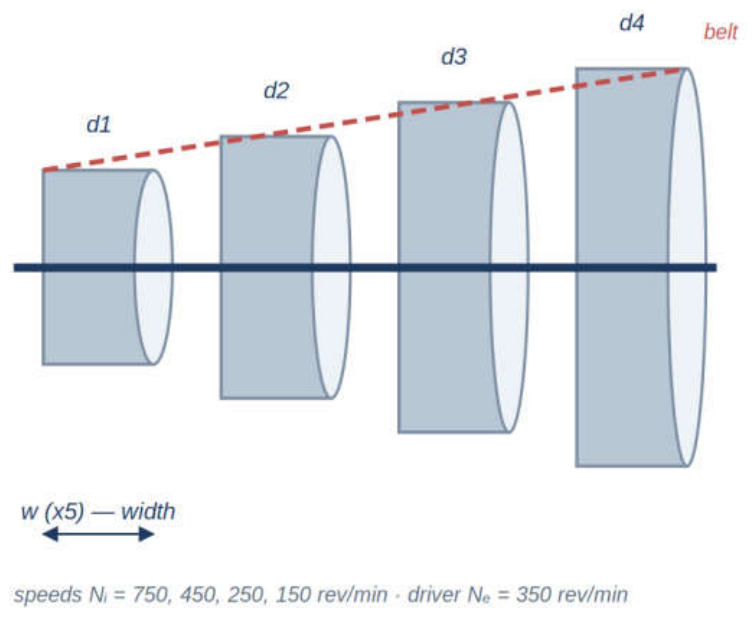
P21 — Planetary gear train (simplified)
| Goal: | Minimize the maximum gear-ratio error of a two-stage planetary gear train across three required operating ratios. The formulation implemented here is a simplified six-variable version using tooth counts only (see Figure L19). |
| Variables: | (). tooth counts of the six gears, integers within problem-specific bounds and rounded inside the objective. |
| Objective: |
|
| Constraints (4) | The meshing-compatibility condition (), a planet-fit condition, a stage-1 size condition and a size-proportion condition. |
| Reference optimum: | 0.525 (approximate). |
| Source: | simplified from (Kumar et al., 2020) Note: P21 is explicitly a simplified 6-variable version; the Kumar formulation has 9 variables. |
Figure L19.
Planetary gear train (simplified). Sun gear , three planets and ring gear , with the meshing condition ; the objective is the largest deviation from the three target ratios.
Figure L19.
Planetary gear train (simplified). Sun gear , three planets and ring gear , with the meshing condition ; the objective is the largest deviation from the three target ratios.
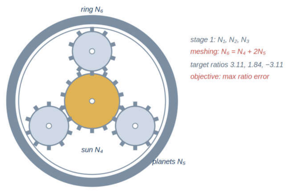
L.2.3 Process and Vehicle Design Problems
P11 — Car side impact
| Goal: | Minimize the weight of a vehicle side structure while satisfying the safety requirements of a side-impact test, expressed as limits on the deflections and velocities measured at the abdomen, ribs and pubic symphysis of a dummy occupant (see Figure L20). |
| Variables: | (). thicknesses of seven structural members two discrete material choices, each selected from two standard values; two barrier-position parameters |
| Objective: |
|
| Constraints (10) | Abdomen load, upper/middle/lower rib deflections, upper/middle/lower viscous criteria, pubic-symphysis force, B-pillar velocity and front-door velocity, each expressed as a response-surface polynomial fitted to crash simulations. |
| Reference optimum: | 22.84296954 |
| Source: | (Talatahari, Azizi, et al., 2021) |
Figure L20.
Car side impact. Side structure showing the , door beam and roof rail whose thicknesses form , with the impacting barrier and the dummy at which the safety responses are measured; the objective is structural weight.
Figure L20.
Car side impact. Side structure showing the , door beam and roof rail whose thicknesses form , with the impacting barrier and the dummy at which the safety responses are measured; the objective is structural weight.
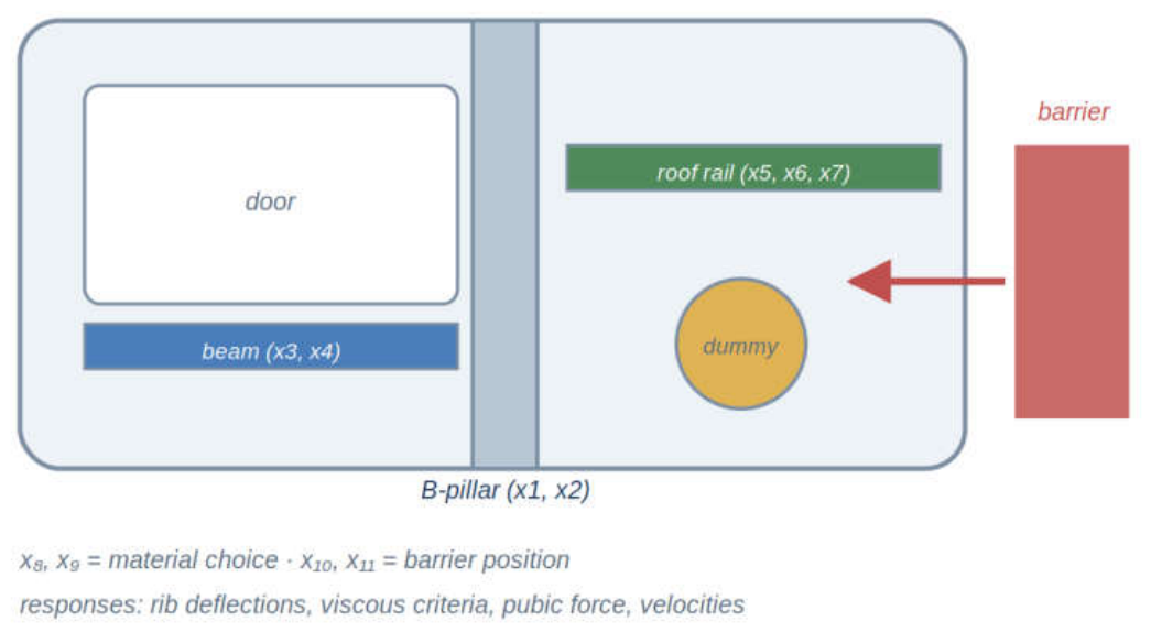
P19 — Gas transmission compressor
| Goal: | Minimize the total annual cost of a gas transmission network, comprising compressor capital cost, pipeline cost and operating cost (see Figure L21). |
| Variables: | (). representing pipeline length, compression ratio, pipe diameter and inlet-pressure parameters in the standard scaled form |
| Objective: | |
| Constraints (1) | A single operating condition linking and |
| Reference optimum: | 2.9649 × 10⁶ |
| Source: | (Kumar et al., 2020) |
Figure L21.
Gas transmission compressor. Pipeline with compressor stations, parameterized by segment length, compression ratio, pipe diameter and inlet pressure; the objective is total annual capital, pipeline and operating cost.
Figure L21.
Gas transmission compressor. Pipeline with compressor stations, parameterized by segment length, compression ratio, pipe diameter and inlet pressure; the objective is total annual capital, pipeline and operating cost.
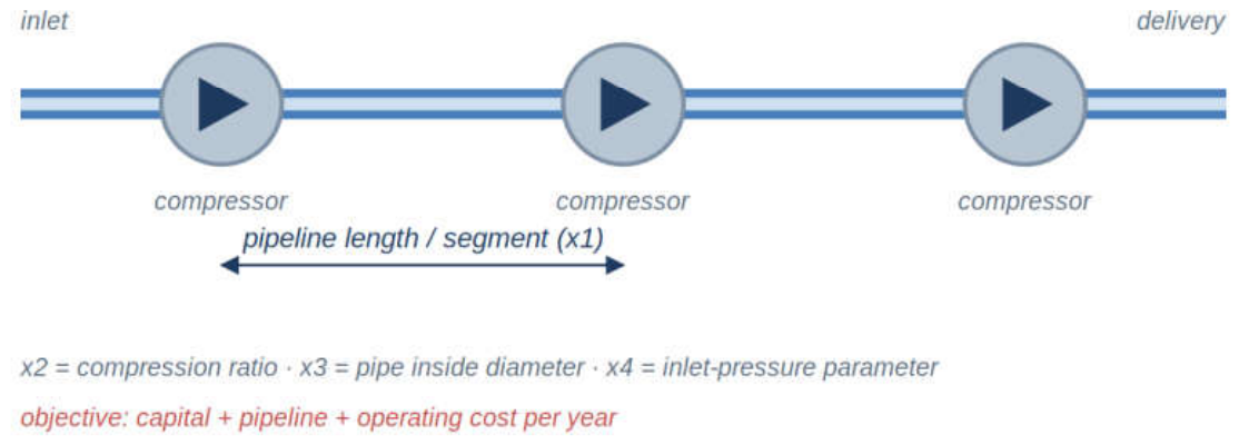
P23 — Heat exchanger design
| Goal: | Minimize the total heat-transfer area of a three-stage heat-exchanger network, the classical Himmelblau formulation (see Figure L22). |
| Variables: | (). = the three exchanger areas and = five intermediate stream temperatures |
| Objective: |
|
| Constraints (6) | Three linear temperature-approach conditions and three bilinear heat-balance conditions coupling areas and temperatures. |
| Reference optimum: | 7049.248 |
| Source: | (Kumar et al., 2020) |
Figure L22.
Heat exchanger design. Three-stage exchanger network with areas and intermediate stream temperatures ; the objective is the total heat-transfer area.
Figure L22.
Heat exchanger design. Three-stage exchanger network with areas and intermediate stream temperatures ; the objective is the total heat-transfer area.
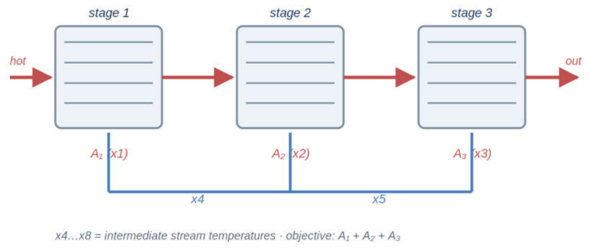
L.3 Aggregate Results Across the Suite
The three tables below summaries the performance of all 43 algorithms over the twenty-two applications documented in Section L.2. Table L1 gives the overall standing, Table L2 the per-problem means for the leading algorithms, and Table L3 the pairwise statistical record of PAO against each competitor.
Table L1.
Complete ranking of all 43 algorithms on the engineering suite: average rank across the twenty-two problems, number of problems won, and Wilcoxon record against PAO.
Table L1.
Complete ranking of all 43 algorithms on the engineering suite: average rank across the twenty-two problems, number of problems won, and Wilcoxon record against PAO.
| # | Algorithm | Average rank | Problems won | W | T | L |
| 1 | PAO | 2.955 | 6 | -- | -- | -- |
| 2 | APO | 4.455 | 4 | 12 | 1 | 9 |
| 3 | GOA | 6.841 | 0 | 19 | 1 | 2 |
| 4 | SFOA | 8.341 | 1 | 19 | 1 | 2 |
| 5 | PGA | 8.886 | 1 | 14 | 3 | 5 |
| 6 | DHOLE | 11.136 | 0 | 19 | 3 | 0 |
| 7 | RFO | 11.455 | 1 | 21 | 0 | 1 |
| 8 | NDO | 11.523 | 0 | 19 | 1 | 2 |
| 9 | YDSE | 12.068 | 0 | 20 | 1 | 1 |
| 10 | SO | 12.091 | 0 | 17 | 2 | 3 |
| 11 | DE | 13.045 | 0 | 16 | 1 | 5 |
| 12 | FOA | 13.568 | 0 | 19 | 3 | 0 |
| 13 | AOA | 13.727 | 0 | 17 | 3 | 2 |
| 14 | EHO | 14.250 | 0 | 16 | 1 | 5 |
| 15 | PSO | 14.523 | 0 | 17 | 3 | 2 |
| 16 | WUTP | 16.068 | 0 | 21 | 0 | 1 |
| 17 | HBA | 16.318 | 0 | 17 | 3 | 2 |
| 18 | SPIBA | 17.273 | 0 | 22 | 0 | 0 |
| 19 | CS | 17.318 | 0 | 21 | 1 | 0 |
| 20 | FPA | 17.455 | 0 | 21 | 0 | 1 |
| 21 | GWO | 20.273 | 0 | 22 | 0 | 0 |
| 22 | MSO | 20.614 | 0 | 20 | 1 | 1 |
| 23 | FOX | 20.636 | 0 | 21 | 1 | 0 |
| 24 | SHS | 20.818 | 0 | 17 | 3 | 2 |
| 25 | DSWO | 22.227 | 0 | 22 | 0 | 0 |
| 26 | GOOSE | 22.773 | 0 | 22 | 0 | 0 |
| 27 | SOA | 23.227 | 0 | 21 | 0 | 1 |
| 28 | ZOA | 23.455 | 0 | 21 | 1 | 0 |
| 29 | WAA | 27.545 | 0 | 22 | 0 | 0 |
| 30 | AO | 30.136 | 0 | 22 | 0 | 0 |
| 31 | WSO | 30.500 | 0 | 22 | 0 | 0 |
| 32 | Chimp | 32.000 | 0 | 22 | 0 | 0 |
| 33 | CPO | 32.045 | 0 | 22 | 0 | 0 |
| 34 | DOA | 33.318 | 0 | 22 | 0 | 0 |
| 35 | TSO | 33.909 | 0 | 22 | 0 | 0 |
| 36 | MRSO | 34.273 | 0 | 22 | 0 | 0 |
| 37 | HS | 36.636 | 0 | 22 | 0 | 0 |
| 38 | MRA | 37.091 | 0 | 22 | 0 | 0 |
| 39 | EMRA | 37.273 | 0 | 22 | 0 | 0 |
| 40 | DRA | 39.364 | 0 | 22 | 0 | 0 |
| 41 | SHO | 40.273 | 0 | 22 | 0 | 0 |
| 42 | CSA | 41.818 | 0 | 22 | 0 | 0 |
| 43 | DAOA | 42.500 | 0 | 22 | 0 | 0 |
Table L2.
Mean fitness (standard deviation) over 30 runs for PAO and the five leading algorithms on each engineering problem, with PAO’s per-problem rank. A feasible design has fitness equal to its objective value.
Table L2.
Mean fitness (standard deviation) over 30 runs for PAO and the five leading algorithms on each engineering problem, with PAO’s per-problem rank. A feasible design has fitness equal to its objective value.
| # | PAO | APO | GOA | SFOA | PGA | DHOLE | PAO rank |
| P01 | 2994.42 (2.3126 × 10⁻¹²) | 2994.42 (1.3953 × 10⁻⁶) | 2994.44 (0.0076595) | 2994.42 (7.3368 × 10⁻¹⁰) | 2994.42 (2.3126 × 10⁻¹²) | 2994.42 (1.2120 × 10⁻⁷) | 3 |
| P02 | 0.0126653 (3.4059 × 10⁻⁷) | 0.0126652 (6.2057 × 10⁻⁸) | 0.0126666 (8.1517 × 10⁻⁷) | 0.0126672 (9.7934 × 10⁻⁶) | 0.0127164 (2.6784 × 10⁻⁵) | 0.0127311 (4.0747 × 10⁻⁵) | 3 |
| P03 | 6059.71 (9.2504 × 10⁻¹³) | 6059.71 (9.2504 × 10⁻¹³) | 6059.75 (0.0370448) | 6061.06 (3.40385) | 6119.15 (233.345) | 6219.34 (272.153) | 1.5 |
| P04 | 263.896 (0) | 263.896 (0) | 263.896 (9.4288 × 10⁻¹³) | 263.896 (1.1051 × 10⁻¹¹) | 263.896 (3.3854 × 10⁻⁶) | 263.896 (5.4788 × 10⁻⁸) | 1.5 |
| P05 | 9.0149 × 10⁻¹¹ (2.4796 × 10⁻¹⁰) | 4.7386 × 10⁻¹² (6.2177 × 10⁻¹²) | 1.6286 × 10⁻¹¹ (9.7702 × 10⁻¹²) | 3.8684 × 10⁻¹⁰ (4.5588 × 10⁻¹⁰) | 6.4586 × 10⁻¹⁰ (6.0447 × 10⁻¹⁰) | 3.8333 × 10⁻¹⁰ (6.7455 × 10⁻¹⁰) | 5 |
| P06 | 1.33996 (2.4740 × 10⁻¹⁶) | 1.33996 (1.1276 × 10⁻¹⁰) | 1.33997 (7.0322 × 10⁻⁶) | 1.34016 (1.9027 × 10⁻⁴) | 1.33997 (1.5722 × 10⁻⁵) | 1.33996 (7.2084 × 10⁻⁶) | 1 |
| P07 | 0.0130741 (7.3809 × 10⁻¹⁸) | 0.0130741 (7.6871 × 10⁻¹¹) | 0.0130741 (5.4874 × 10⁻¹⁰) | 0.0130741 (6.3125 × 10⁻¹³) | 0.0130741 (8.8219 × 10⁻¹⁸) | 0.0130741 (6.1708 × 10⁻¹⁰) | 7 |
| P08 | 26.4864 (0) | 26.4864 (0) | 26.4864 (2.3615 × 10⁻⁸) | 26.4864 (1.8248 × 10⁻⁸) | 26.4864 (0) | 26.4864 (9.4624 × 10⁻¹²) | 6.5 |
| P09 | 29.6207 (54.9944) | 45.5268 (68.4249) | 8.41271 (8.1494 × 10⁻⁶) | 40.5011 (64.5891) | 8.4127 (8.4406 × 10⁻¹⁴) | 87.9427 (80.8896) | 8 |
| P11 | 22.843 (7.4969 × 10⁻¹²) | 22.845 (6.5101 × 10⁻⁴) | 22.8461 (0.00163252) | 22.9125 (0.138082) | 22.9085 (0.126325) | 23.154 (0.214132) | 1 |
| P12 | 1.72485 (1.1292 × 10⁻¹⁵) | 1.72485 (1.0013 × 10⁻¹²) | 1.72507 (1.1654 × 10⁻⁴) | 1.72541 (2.8752 × 10⁻⁴) | 1.72485 (2.5277 × 10⁻¹⁵) | 1.72485 (9.4294 × 10⁻⁸) | 1 |
| P13 | 359.208 (0) | 359.208 (0) | 359.208 (5.6541 × 10⁻¹¹) | 359.208 (1.3726 × 10⁻⁸) | 359.309 (0.555391) | 359.322 (0.625499) | 2 |
| P14 | 0.313657 (1.6938 × 10⁻¹⁶) | 0.313657 (2.0170 × 10⁻¹⁴) | 0.313657 (2.0690 × 10⁻⁹) | 0.313657 (4.6151 × 10⁻¹²) | 0.313657 (1.6938 × 10⁻¹⁶) | 0.313657 (2.5355 × 10⁻¹⁶) | 4 |
| P15 | -82842.2 (0) | -82842.2 (0.00102013) | -82842.2 (3.0090 × 10⁻⁴) | -82842.2 (0) | -82842.2 (0) | -82842.2 (1.1356 × 10⁻¹⁰) | 4 |
| P16 | 1.97967 (1.2815 × 10⁻¹⁵) | 1.97968 (2.4026 × 10⁻⁷) | 1.98843 (0.00573508) | 2.03094 (0.0518356) | 2.03722 (0.0404371) | 2.00939 (0.0354996) | 1 |
| P17 | 19733.1 (392.137) | 19506.4 (0.959108) | 21837.7 (659.581) | 22396 (1084.26) | 25929.8 (4606.67) | 29553.4 (4200.42) | 2 |
| P18 | 4.34957 (0.0105126) | 4.45012 (0.020842) | 4.40962 (0.0891989) | 4.31925 (0.151032) | 4.68554 (0.228226) | 4.67646 (0.345202) | 2 |
| P19 | 2.2927 × 10⁶ (2.4381 × 10⁻⁹) | 2.2927 × 10⁶ (6.0530 × 10⁻¹⁰) | 2.2927 × 10⁶ (1.3590 × 10⁻⁹) | 2.2927 × 10⁶ (2.2316 × 10⁻⁹) | 2.2927 × 10⁶ (1.4877 × 10⁻⁹) | 2.2927 × 10⁶ (3.5569 × 10⁻⁹) | 3.5 |
| P20 | 16.2083 (0.657597) | 16.1358 (0.227286) | 19.443 (2.51685) | 38.2395 (31.9779) | 85.8071 (30.5486) | 72.1981 (30.8721) | 2 |
| P21 | 0.525549 (0.00130009) | 0.524212 (0.0012202) | 0.524753 (0.00138943) | 0.525607 (0.00290457) | 0.53171 (0.00519991) | 0.529604 (0.00670522) | 4 |
| P22 | 5060.85 (2.9395 × 10⁻⁸) | 5061.33 (0.150049) | 5062.44 (0.996108) | 5061.57 (2.85851) | 5063.41 (5.59642) | 5066.55 (7.70656) | 1 |
| P23 | 7049.25 (0.00280736) | 7069.45 (9.15742) | 7414.93 (114.975) | 7503.61 (114.054) | 7785.67 (558.056) | 7542.2 (341.235) | 1 |
Table L3.
PAO versus each competitor on the engineering suite: Wilcoxon rank-sum wins (W), ties (T) and losses (L) for PAO across the twenty-two problems, with net score (W−L). Sorted from PAO’s largest advantage. PAO is net-positive against all 42 competitors, including APO (12–1–9).
Table L3.
PAO versus each competitor on the engineering suite: Wilcoxon rank-sum wins (W), ties (T) and losses (L) for PAO across the twenty-two problems, with net score (W−L). Sorted from PAO’s largest advantage. PAO is net-positive against all 42 competitors, including APO (12–1–9).
| Competitor | W | T | L | Net | Competitor | W | T | L | Net | |
| AO | 22 | 0 | 0 | +22 | ZOA | 21 | 1 | 0 | +21 | |
| CPO | 22 | 0 | 0 | +22 | FPA | 21 | 0 | 1 | +20 | |
| CSA | 22 | 0 | 0 | +22 | RFO | 21 | 0 | 1 | +20 | |
| Chimp | 22 | 0 | 0 | +22 | SOA | 21 | 0 | 1 | +20 | |
| DAOA | 22 | 0 | 0 | +22 | WUTP | 21 | 0 | 1 | +20 | |
| DOA | 22 | 0 | 0 | +22 | MSO | 20 | 1 | 1 | +19 | |
| DRA | 22 | 0 | 0 | +22 | YDSE | 20 | 1 | 1 | +19 | |
| DSWO | 22 | 0 | 0 | +22 | DHOLE | 19 | 3 | 0 | +19 | |
| EMRA | 22 | 0 | 0 | +22 | FOA | 19 | 3 | 0 | +19 | |
| GOOSE | 22 | 0 | 0 | +22 | GOA | 19 | 1 | 2 | +17 | |
| GWO | 22 | 0 | 0 | +22 | NDO | 19 | 1 | 2 | +17 | |
| HS | 22 | 0 | 0 | +22 | SFOA | 19 | 1 | 2 | +17 | |
| MRA | 22 | 0 | 0 | +22 | AOA | 17 | 3 | 2 | +15 | |
| MRSO | 22 | 0 | 0 | +22 | HBA | 17 | 3 | 2 | +15 | |
| SHO | 22 | 0 | 0 | +22 | PSO | 17 | 3 | 2 | +15 | |
| SPIBA | 22 | 0 | 0 | +22 | SHS | 17 | 3 | 2 | +15 | |
| TSO | 22 | 0 | 0 | +22 | SO | 17 | 2 | 3 | +14 | |
| WAA | 22 | 0 | 0 | +22 | DE | 16 | 1 | 5 | +11 | |
| WSO | 22 | 0 | 0 | +22 | EHO | 16 | 1 | 5 | +11 | |
| CS | 21 | 1 | 0 | +21 | PGA | 14 | 3 | 5 | +9 | |
| FOX | 21 | 1 | 0 | +21 | APO | 12 | 1 | 9 | +3 |
Note on reference values. The reference optima of Table 23 are best-known values from literature. For problems P15, P16, P18, P20 and P21 the source implementation states that reported values vary between publications and should be treated as targets rather than exact optima; for P21 the formulation is a simplified planetary model. On P05, P14, P17 and P18 no algorithm in the pool of 43 attains the tabulated value, which indicates a discrepancy between the coded formulation and the cited reference rather than a limitation of any individual optimizer. Comparisons between algorithms remain valid throughout, because every algorithm optimizes the same coded formulation under the same penalty wrapper.
L.4 Material Held in the Result Archive
The following per-problem material supports Section L.3 but is too extensive to reproduce in the document. It is distributed with the result archive, and the file and sheet holding each item is named so that any figure in Section 6 can be regenerated.
| Item | Content | Source |
| Full statistics | Mean, standard deviation, best, worst and median over 30 runs, all 43 algorithms × 22 applications | Statistics.xlsx, sheet Summary |
| Raw runs | Every individual run of every algorithm on every application | RawData.xlsx |
| Rank matrix | Per-problem ranks, average rank, overall position, Friedman ANOVA | Ranks.xlsx |
| Wilcoxon detail | p-values and win/tie/loss verdicts, PAO against each of the 42 competitors on every application | Pvalues.xlsx |
| Best designs | Best design-variable vectors per algorithm per application, mapped back to physical units | EngineeringOptima.xlsx, sheets Design_* |
| Runtime | Mean and total wall-clock time per algorithm per application, with the speed ranking | Time.xlsx |
| Convergence curves | Mean best-so-far curves over 500 iterations, all algorithms, one panel per application | Convergence Figures/ |
References
- Abdel-Basset, M., El-Shahat, D., Jameel, M., & Abouhawwash, M. (2023). Young’s double-slit experiment optimizer : A novel metaheuristic optimization algorithm for global and constraint optimization problems. Computer Methods in Applied Mechanics and Engineering, 403, 115652. [CrossRef]
- Abdulla, H. S., Ameen, A. A., Saeed, S. I., Mohammed, I. A., & Rashid, T. A. (2024). MRSO: Balancing Exploration and Exploitation through Modified Rat Swarm Optimization for Global Optimization. Algorithms, 17(9). [CrossRef]
- Abualigah, L., Sheikhan, A., M. Ikotun, A., Zitar, R. A., Alsoud, A. R., Al-Shourbaji, I., Hussien, A. G., & Jia, H. (2024). 1 - Particle swarm optimization algorithm: review and applications (L. B. T.-M. O. A. Abualigah, Ed.; pp. 1–14). Morgan Kaufmann. [CrossRef]
- Abualigah, L., Yousri, D., Abd Elaziz, M., Ewees, A. A., Al-qaness, M. A. A., & Gandomi, A. H. (2021). Aquila Optimizer: A novel meta-heuristic optimization algorithm. Computers & Industrial Engineering, 157, 107250. [CrossRef]
- Agrawal, P., Abutarboush, H. F., Ganesh, T., & Mohamed, A. W. (2021). Metaheuristic Algorithms on Feature Selection: A Survey of One Decade of Research (2009-2019). IEEE Access, 9, 26766–26791. [CrossRef]
- Agushaka, J. O., Ezugwu, A. E., & Abualigah, L. (2023). Gazelle optimization algorithm: a novel nature-inspired metaheuristic optimizer. Neural Computing and Applications, 35(5), 4099–4131. [CrossRef]
- Akbari, E., Rahimnejad, A., & Gadsden, S. A. (2025). Holistic swarm optimization: A novel metaphor-less algorithm guided by whole population information for addressing exploration-exploitation dilemma. Computer Methods in Applied Mechanics and Engineering, 445, 118208. [CrossRef]
- Al-Betar, M. A., Awadallah, M. A., Braik, M. S., Makhadmeh, S., & Doush, I. A. (2024). Elk herd optimizer: a novel nature-inspired metaheuristic algorithm. Artificial Intelligence Review, 57(3), 48.
- Al-Tashi, Q., Kadir, S. J. A., Rais, H. M., Mirjalili, S., & Alhussian, H. (2019). Binary Optimization Using Hybrid Grey Wolf Optimization for Feature Selection. IEEE Access, 7, 39496–39508. [CrossRef]
- Alba, E. (2005). Parallel metaheuristics: a new class of algorithms. John Wiley & Sons.
- Ali, S. K., & Ameen, A. A. (2025). A Performance-Driven Enhancement of the Mud Ring Algorithm for Global Optimization Challenges. Kurdistan Journal of Applied Research, 10(2), 178–211. [CrossRef]
- Ameen, A. A. (2024). Metaheuristic Optimazation Algorithms in Applied Science and Engineering Applications.pdf [Erbil Polytechnic University]. https://epu.edu.iq/2024/03/17/metaheuristic-optimization-algorithms-in-applied-science-and-engineering-applications-2/.
- Ameen, A. A., Rashid, T. A., & Askar, S. (2023). CDDO-HS: Child Drawing Development Optimization-Harmony Search Algorithm. In Applied Sciences (Vol. 13, Number 9). [CrossRef]
- Ameen, A. A., Rashid, T. A., & Askar1, S. (2023). A Tutorial on Child Drawing Development. Proceedings of the 1st International Conference on Innovation in Information Technology and Business (ICIITB 2022), 153.
- Aranha, C., Camacho Villalón, C. L., Campelo, F., Dorigo, M., Ruiz, R., Sevaux, M., Sörensen, K., & Stützle, T. (2022). Metaphor-based metaheuristics, a call for action: the elephant in the room. Swarm Intelligence, 16(1), 1–6. [CrossRef]
- Ayyarao, T. S. L. V, Ramakrishna, N. S. S., Elavarasan, R. M., Polumahanthi, N., Rambabu, M., Saini, G., Khan, B., & Alatas, B. (2022). War Strategy Optimization Algorithm: A New Effective Metaheuristic Algorithm for Global Optimization. IEEE Access, 10, 25073–25105. [CrossRef]
- Bahri, S. A., & Hasibuan, S. (2024). Muslim Prayer Times on Astronomy and Fuqaha. Al-Hisab: Journal of Islamic Astronomy, 1(4), 163–173.
- Blum, C., & Roli, A. (2003). Metaheuristics in Combinatorial Optimization: Overview and Conceptual Comparison. ACM Comput. Surv., 35(3), 268–308. [CrossRef]
- Bohat, V. K., Hashim, F. A., Batra, H., & Abd Elaziz, M. (2025). Phototropic growth algorithm: A novel metaheuristic inspired from phototropic growth of plants. Knowledge-Based Systems, 322, 113548. [CrossRef]
- Boussaïd, I., Lepagnot, J., & Siarry, P. (2013). A survey on optimization metaheuristics. Information Sciences, 237, 82–117. [CrossRef]
- Braik, M., & Al-Hiary, H. (2025a). A novel meta-heuristic optimization algorithm inspired by water uptake and transport in plants. Neural Computing and Applications, 37(19), 13643–13724. [CrossRef]
- Braik, M., & Al-Hiary, H. (2025b). Rüppell’s fox optimizer: A novel meta-heuristic approach for solving global optimization problems. Cluster Computing, 28(5), 292. [CrossRef]
- Burke, E. K., Gendreau, M., Hyde, M., Kendall, G., Ochoa, G., Özcan, E., & Qu, R. (2013). Hyper-heuristics: a survey of the state of the art. Journal of the Operational Research Society, 64(12), 1695–1724. [CrossRef]
- Chakraborty, S., Saha, A. K., Ezugwu, A. E., Agushaka, J. O., Zitar, R. A., & Abualigah, L. (2023). Differential Evolution and Its Applications in Image Processing Problems: A Comprehensive Review. Archives of Computational Methods in Engineering, 30(2), 985–1040. [CrossRef]
- Cheng, J., & De Waele, W. (2024). Weighted average algorithm: A novel meta-heuristic optimization algorithm based on the weighted average position concept. Knowledge-Based Systems, 305, 112564. [CrossRef]
- Coello, C. A. C., Pulido, G. T., & Lechuga, M. S. (2004). Handling multiple objectives with particle swarm optimization. IEEE Transactions on Evolutionary Computation, 8(3), 256–279. [CrossRef]
- Coello Coello, C. A. (2002). Theoretical and numerical constraint-handling techniques used with evolutionary algorithms: a survey of the state of the art. Computer Methods in Applied Mechanics and Engineering, 191(11), 1245–1287. [CrossRef]
- Cooper, P. I. (1969). The absorption of radiation in solar stills. Solar Energy, 12(3), 333–346. [CrossRef]
- Darvishpoor, S., Darvishpour, A., Escarcega, M., & Hassanalian, M. (2023). Nature-Inspired Algorithms from Oceans to Space: A Comprehensive Review of Heuristic and Meta-Heuristic Optimization Algorithms and Their Potential Applications in Drones. Drones, 7(7), 427.
- Deb, K., & Jain, H. (2014). An Evolutionary Many-Objective Optimization Algorithm Using Reference-Point-Based Nondominated Sorting Approach, Part I: Solving Problems With Box Constraints. IEEE Transactions on Evolutionary Computation, 18(4), 577–601. [CrossRef]
- Deb, K., Pratap, A., Agarwal, S., & Meyarivan, T. (2002). A fast and elitist multiobjective genetic algorithm: NSGA-II. IEEE Transactions on Evolutionary Computation, 6(2), 182–197. [CrossRef]
- Demšar, J. (2006). Statistical comparisons of classifiers over multiple data sets. Journal of Machine Learning Research, 7(Jan), 1–30.
- Derrac, J., García, S., Molina, D., & Herrera, F. (2011). A practical tutorial on the use of nonparametric statistical tests as a methodology for comparing evolutionary and swarm intelligence algorithms. Swarm and Evolutionary Computation, 1(1), 3–18. [CrossRef]
- Desuky, A. S., Cifci, M. A., Kausar, S., Hussain, S., & El Bakrawy, L. M. (2022). Mud Ring Algorithm: A new meta-heuristic optimization algorithm for solving mathematical and engineering challenges. IEEE Access, 10, 50448–50466.
- Dhiman, G. (2021). SSC: A hybrid nature-inspired meta-heuristic optimization algorithm for engineering applications. Knowledge-Based Systems, 222, 106926.
- Dhiman, G., & Kumar, V. (2017). Spotted hyena optimizer: A novel bio-inspired based metaheuristic technique for engineering applications. Advances in Engineering Software, 114, 48–70. [CrossRef]
- Dorigo, M. (2020). Grey Wolf, Firefly and Bat Algorithms: Three Widespread Algorithms that. Swarm Intelligence: 12th International Conference, ANTS 2020, Barcelona, Spain, October 26–28, 2020, Proceedings, 121.
- Duffie, J. A., & Beckman, W. A. (2013). Solar engineering of thermal processes. John Wiley & Sons.
- Eiben, A. E., Hinterding, R., & Michalewicz, Z. (1999). Parameter control in evolutionary algorithms. IEEE Transactions on Evolutionary Computation, 3(2), 124–141. [CrossRef]
- Esposito, J. L. (2011). What everyone needs to know about Islam. Oxford University Press.
- Faraj, A. K., Aladdin, A. M. M., & Ameen, A. A. A. (2025). EESB-FDO: enhancing the fitness-dependent optimizer through a modified boundary handling mechanism. Frontiers in Applied Mathematics and Statistics, Volume 11. https://www.frontiersin.org/journals/applied-mathematics-and-statistics/articles/10.3389/fams.2025.1640044.
- Fister, I., Yang, X.-S., Fister, I., Brest, J., & Fister, D. (2013). A Brief Review of Nature-Inspired Algorithms for Optimization. Elektrotehniski Vestnik/Electrotechnical Review.
- Ghaemifard, S., & Ghannadiasl, A. (2024). A Comparison of Metaheuristic Algorithms for Structural Optimization: Performance and Efficiency Analysis. Advances in Civil Engineering, 2024(1), 2054173. [CrossRef]
- Givi, H., & Hubalovska, M. (2023). Skill Optimization Algorithm: A New Human-Based Metaheuristic Technique. In Computers, Materials \& Continua (Vol. 74, Number 1). [CrossRef]
- Guo, Z., Liu, G., & Jiang, F. (2025). Chinese Pangolin Optimizer: a novel bio-inspired metaheuristic for solving optimization problems. The Journal of Supercomputing, 81(4), 517. [CrossRef]
- Gupta, S., & Deep, K. (2019). A novel Random Walk Grey Wolf Optimizer. Swarm and Evolutionary Computation, 44, 101–112. [CrossRef]
- Hamad, R. K., & Rashid, T. A. (2024). GOOSE algorithm: a powerful optimization tool for real-world engineering challenges and beyond. Evolving Systems, 15(4), 1249–1274. [CrossRef]
- Hamadneh, T., Batiha, B., Werner, F., Montazeri, Z., Dehghani, M., Bektemyssova, G., & Eguchi, K. (2024). Fossa Optimization Algorithm: A New Bio-Inspired Metaheuristic Algorithm for Engineering Applications. International Journal of Intelligent Engineering and Systems, 17(5), 1038–1047. [CrossRef]
- Hamajan, K. F. (2026). Journal of Studies in Science and Engineering Heart Disease Prediction Using Machine Learning with Greater Cane Rat Algorithm-Based Hyperparameter Tuning. 6(1), 365–394.
- Hamid, N. K., Ameen, A. A. A., & Aladdin, A. M. M. (2026). EMRSO: enhancing the modified rat swarm optimizer via hybrid memory strategies. Frontiers in Applied Mathematics and Statistics, Volume 12. https://www.frontiersin.org/journals/applied-mathematics-and-statistics/articles/10.3389/fams.2026.1838903.
- Hasan, D. O., & Aladdin, A. (2025). Real-world applications of metaheuristic algorithms: a comprehensive review of the state-of-the-art. Diyala Journal of Engineering Sciences, 1–27.
- Hashim, F. A., Houssein, E. H., Hussain, K., Mabrouk, M. S., & Al-Atabany, W. (2022). Honey Badger Algorithm: New metaheuristic algorithm for solving optimization problems. Mathematics and Computers in Simulation, 192, 84–110. [CrossRef]
- Hashim, F. A., Hussain, K., Houssein, E. H., Mabrouk, M. S., & Al-Atabany, W. (2021). Archimedes optimization algorithm: a new metaheuristic algorithm for solving optimization problems. Applied Intelligence, 51(3), 1531–1551. [CrossRef]
- Hashim, F. A., & Hussien, A. G. (2022). Snake Optimizer: A novel meta-heuristic optimization algorithm. Knowledge-Based Systems, 242, 108320. [CrossRef]
- He, J., Zhao, S., Ding, J., & Wang, Y. (2025). Mirage search optimization: Application to path planning and engineering design problems. Advances in Engineering Software, 203, 103883. [CrossRef]
- Hegazy, A. E., Makhlouf, M. A., & El-Tawel, G. S. (2020). Improved salp swarm algorithm for feature selection. Journal of King Saud University - Computer and Information Sciences, 32(3), 335–344. [CrossRef]
- Helmi, A. M., Al-qaness, M. A. A., Dahou, A., Damaševičius, R., Krilavičius, T., & Elaziz, M. A. (2021). A Novel Hybrid Gradient-Based Optimizer and Grey Wolf Optimizer Feature Selection Method for Human Activity Recognition Using Smartphone Sensors. In Entropy (Vol. 23, Number 8, p. 1065). [CrossRef]
- Himmelblau, D. M. (1972). A uniform evaluation of unconstrained optimization techniques. Academic Press.
- Houssein, E. H., Emam, M. M., & Ali, A. A. (2021). Improved manta ray foraging optimization for multi-level thresholding using COVID-19 CT images. Neural Computing and Applications, 33(24), 16899–16919. [CrossRef]
- Houssein, E. H., Hossam Abdel Gafar, M., Fawzy, N., & Sayed, A. Y. (2025). Recent metaheuristic algorithms for solving some civil engineering optimization problems. Scientific Reports, 15(1), 7929. [CrossRef]
- Jaddi, N. S., & Abdullah, S. (2020). Global search in single-solution-based metaheuristics. Data Technologies and Applications, 54(3), 275–296.
- Kaveh, A., & Sabzi, O. (2011). A comparative study of two meta-heuristic algorithms for optimum design of reinforced concrete frames.
- Kennedy, J., & Eberhart, R. (1995). Particle swarm optimization. Proceedings of ICNN’95 - International Conference on Neural Networks, 4, 1942–1948 vol.4. [CrossRef]
- Khishe, M., & Mosavi, M. R. (2020). Chimp optimization algorithm. Expert Systems with Applications, 149, 113338. [CrossRef]
- Khodadadi, N., Snasel, V., & Mirjalili, S. (2022). Dynamic Arithmetic Optimization Algorithm for Truss Optimization Under Natural Frequency Constraints. IEEE Access, 10, 16188–16208. [CrossRef]
- Khoshniat, N., Jamarani, A., Ahmadzadeh, A., Haghi Kashani, M., & Mahdipour, E. (2024). Nature-inspired metaheuristic methods in software testing. Soft Computing, 28(2), 1503–1544. [CrossRef]
- Kumar, A., Wu, G., Ali, M. Z., Mallipeddi, R., Suganthan, P. N., & Das, S. (2020). A test-suite of non-convex constrained optimization problems from the real-world and some baseline results. Swarm and Evolutionary Computation, 56, 100693. [CrossRef]
- Lang, Y., & Gao, Y. (2025). Dream Optimization Algorithm (DOA): A novel metaheuristic optimization algorithm inspired by human dreams and its applications to real-world engineering problems. Computer Methods in Applied Mechanics and Engineering, 436, 117718. [CrossRef]
- LaTorre, A., Molina, D., Osaba, E., Poyatos, J., Del Ser, J., & Herrera, F. (2021). A prescription of methodological guidelines for comparing bio-inspired optimization algorithms. Swarm and Evolutionary Computation, 67, 100973. [CrossRef]
- Li, G., Zhang, T., Tsai, C.-Y., Yao, L., Lu, Y., & Tang, J. (2024). Review of the metaheuristic algorithms in applications: Visual analysis based on bibliometrics. Expert Systems with Applications, 255, 124857. [CrossRef]
- Ma, C. C. Y., & Iqbal, M. (1983). Statistical comparison of models for estimating solar radiation on inclined surgaces. Solar Energy, 31(3), 313–317. [CrossRef]
- Mafarja, M. M., & Mirjalili, S. (2017). Hybrid Whale Optimization Algorithm with simulated annealing for feature selection. Neurocomputing, 260, 302–312. [CrossRef]
- Meeus, J. H. (1991). Astronomical algorithms. Willmann-Bell, Incorporated.
- Mirjalili, S. (2016). SCA: A Sine Cosine Algorithm for solving optimization problems. Knowledge-Based Systems, 96, 120–133. [CrossRef]
- Mirjalili, S., & Lewis, A. (2013). S-shaped versus V-shaped transfer functions for binary Particle Swarm Optimization. Swarm and Evolutionary Computation, 9, 1–14. [CrossRef]
- Mirjalili, S., Mirjalili, S. M., & Lewis, A. (2014). Grey wolf optimizer. Advances in Engineering Software, 69, 46–61.
- Mirjalili, S., Saremi, S., Mirjalili, S. M., & Coelho, L. dos S. (2016). Multi-objective grey wolf optimizer: A novel algorithm for multi-criterion optimization. Expert Systems with Applications, 47, 106–119. [CrossRef]
- Mohammed, B. O., Aghdasi, H. S., & Salehpour, P. (2025). Dhole optimization algorithm: a new metaheuristic algorithm for solving optimization problems. Cluster Computing, 28(7), 430. [CrossRef]
- Mohammed, H., & Rashid, T. (2023). FOX: a FOX-inspired optimization algorithm. Applied Intelligence, 53(1), 1030–1050. [CrossRef]
- Molina, D., Poyatos, J., Ser, J. Del, García, S., Hussain, A., & Herrera, F. (2020). Comprehensive Taxonomies of Nature- and Bio-inspired Optimization: Inspiration Versus Algorithmic Behavior, Critical Analysis Recommendations. Cognitive Computation, 12(5), 897–939. [CrossRef]
- Mozhdehi, A. T., Khodadadi, N., Aboutalebi, M., El-kenawy, E.-S. M., Hussien, A. G., Zhao, W., Nadimi-Shahraki, M. H., & Mirjalili, S. (2025). Divine Religions Algorithm: a novel social-inspired metaheuristic algorithm for engineering and continuous optimization problems. Cluster Computing, 28(4), 253. [CrossRef]
- Nemati, S., Basiri, M. E., Ghasem-Aghaee, N., & Aghdam, M. H. (2009). A novel ACO–GA hybrid algorithm for feature selection in protein function prediction. Expert Systems with Applications, 36(10), 12086–12094. [CrossRef]
- Omeka, M. E., Ezugwu, A. L., Agbasi, J. C., Egbueri, J. C., Abugu, H. O., Aralu, C. C., & Ucheana, I. A. (2024). A review of the status, challenges, trends, and prospects of groundwater quality assessment in Nigeria: an evidence-based meta-analysis approach. Environmental Science and Pollution Research, 31(15), 22284–22307. [CrossRef]
- Pan, J.-S., Hu, P., Snášel, V., & Chu, S.-C. (2023). A survey on binary metaheuristic algorithms and their engineering applications. Artificial Intelligence Review, 56(7), 6101–6167. [CrossRef]
- Pardo, X. C., González, P., Banga, J. R., Doallo, R., Ayyarao, T. S. L. V, Ramakrishna, N. S. S., Elavarasan, R. M., Polumahanthi, N., Rambabu, M., Saini, G., Khan, B., & Alatas, B. (2024). Population based metaheuristics in Spark: Towards a general framework using PSO as a case study. Swarm and Evolutionary Computation, 10, 101483. [CrossRef]
- Payerle, G., Team, R. C., Payerle, G., D, S., Dolnicar, S., Chapple, A., Pastuszak, A. W., Wang, R., Bi, J., Wang, Z., Yuan, H., Zhang, J., & Zhou, M. (2023). Self-adaptive teaching-learning-based optimizer with improved RBF and sparse autoencoder for high-dimensional problems. Information Sciences, 630(4), 463–481. [CrossRef]
- Pham, V. H. S., Nguyen Dang, N. T., & Nguyen, V. N. (2023). Hybrid Sine Cosine Algorithm with Integrated Roulette Wheel Selection and Opposition-Based Learning for Engineering Optimization Problems. International Journal of Computational Intelligence Systems, 16(1), 171. [CrossRef]
- Price, K. V. (2013). Differential Evolution BT - Handbook of Optimization: From Classical to Modern Approach (I. Zelinka, V. Snášel, & A. Abraham, Eds.; pp. 187–214). Springer Berlin Heidelberg. [CrossRef]
- Price, K. V, Awad, N. H., Ali, M. Z., & Suganthan, P. N. (2018). Problem definitions and evaluation criteria for the 100-digit challenge special session and competition on single objective numerical optimization. In Technical report. Nanyang Technological University Singapore.
- Qais, M. H., Hasanien, H. M., & Alghuwainem, S. (2020). Transient search optimization: a new meta-heuristic optimization algorithm. Applied Intelligence, 50(11), 3926–3941. [CrossRef]
- Qais, M. H., Hasanien, H. M., Turky, R. A., Alghuwainem, S., Tostado-Véliz, M., & Jurado, F. (2022). Circle search algorithm: A geometry-based metaheuristic optimization algorithm. Mathematics, 10(10), 1626.
- Raidl, G. R. (2006). A Unified View on Hybrid Metaheuristics BT - Hybrid Metaheuristics (F. Almeida, M. J. Blesa Aguilera, C. Blum, J. M. Moreno Vega, M. Pérez Pérez, A. Roli, & M. Sampels, Eds.; pp. 1–12). Springer Berlin Heidelberg.
- Rajwar, K., Deep, K., & Das, S. (2023). An exhaustive review of the metaheuristic algorithms for search and optimization: taxonomy, applications, and open challenges. Artificial Intelligence Review. [CrossRef]
- Rojak, E. A., & Fawzi, R. (2024). The Normative Basis of Islamic Astronomy For The Transformation of Prayer Schedules To Digital And Its Accuracy. El-Usrah: Jurnal Hukum Keluarga, 7(2), 602–622.
- S. S., V. C., & H. S., A. (2022). Nature inspired meta heuristic algorithms for optimization problems. Computing, 104(2), 251–269. [CrossRef]
- Safiri, S., & Nikoofard, A. (2023). Ladybug Beetle Optimization algorithm: application for real-world problems. The Journal of Supercomputing, 79(3), 3511–3560. [CrossRef]
- Salgotra, R., Sharma, P., Kundu, K., Raju, S., & Gandomi, A. H. (2025). Enhancing differential evolution algorithm for CEC 2014, CEC 2017, CEC 2021, and CEC 2022 test suites. Neural Computing and Applications, 37(33), 27593–27630. [CrossRef]
- Sayed, G. I., Tharwat, A., & Hassanien, A. E. (2019). Chaotic dragonfly algorithm: an improved metaheuristic algorithm for feature selection. Applied Intelligence, 49(1), 188–205. [CrossRef]
- Şenel, F. A., Gökçe, F., Yüksel, A. S., & Yiğit, T. (2019). A novel hybrid PSO–GWO algorithm for optimization problems. Engineering with Computers, 35(4), 1359–1373. [CrossRef]
- Shaikh, M. S., Raj, S., Zheng, G., Xie, S., Wang, C., Dong, X., Lin, Y., Wang, C., & Junejo, N. U. R. (2025). Applications, classifications, and challenges: a comprehensive evaluation of recently developed metaheuristics for search and analysis. Artificial Intelligence Review, 58(12), 390. [CrossRef]
- Siddique, N., & Adeli, H. (2015). Nature Inspired Computing: An Overview and Some Future Directions. Cognitive Computation, 7(6), 706–714. [CrossRef]
- Singh, A., Mousavi, S. M. H., & Gaurav, K. (2024). SHS: Scorpion Hunting Strategy Swarm Algorithm. ArXiv Preprint ArXiv:2407.14202.
- Sloss, A. N., & Gustafson, S. (2020). 2019 Evolutionary Algorithms Review BT - Genetic Programming Theory and Practice XVII (W. Banzhaf, E. Goodman, L. Sheneman, L. Trujillo, & B. Worzel, Eds.; pp. 307–344). Springer International Publishing. [CrossRef]
- Sörensen, K. (2015). Metaheuristics—the metaphor exposed. International Transactions in Operational Research, 22(1), 3–18. [CrossRef]
- Sörensen, K., & Glover, F. (2013). Metaheuristics. Encyclopedia of Operations Research and Management Science, 62(1), 960–970.
- Sörensen, K., Sevaux, M., & Glover, F. (2025). A History of Metaheuristics. In R. Martí, P. M. Pardalos, & M. G. C. Resende (Eds.), Handbook of Heuristics (pp. 991–1010). Springer Nature Switzerland. [CrossRef]
- Steer, K. C. B., Wirth, A., & Halgamuge, S. K. (2009). The Rationale Behind Seeking Inspiration from Nature BT - Nature-Inspired Algorithms for Optimisation (R. Chiong, Ed.; pp. 51–76). Springer Berlin Heidelberg. [CrossRef]
- Storn, R., & Price, K. (1997). Differential Evolution – A Simple and Efficient Heuristic for global Optimization over Continuous Spaces. Journal of Global Optimization, 11(4), 341–359. [CrossRef]
- Talatahari, S., Azizi, M., Tolouei, M., Talatahari, B., & Sareh, P. (2021). Crystal Structure Algorithm (CryStAl): A Metaheuristic Optimization Method. IEEE Access, 9, 71244–71261. [CrossRef]
- Talatahari, S., Bayzidi, H., & Saraee, M. (2021). Social Network Search for Global Optimization. IEEE Access, 9, 92815–92863. [CrossRef]
- Talbi, E.-G. (2009a). Common Concepts for Metaheuristics. In Metaheuristics (pp. 1–86). [CrossRef]
- Talbi, E.-G. (2009b). Metaheuristics: from design to implementation. John Wiley & Sons.
- Tanabe, R., & Fukunaga, A. S. (2014). Improving the search performance of SHADE using linear population size reduction. 2014 IEEE Congress on Evolutionary Computation (CEC), 1658–1665. [CrossRef]
- Trojovská, E., Dehghani, M., & Trojovský, P. (2022). Zebra Optimization Algorithm: A New Bio-Inspired Optimization Algorithm for Solving Optimization Algorithm. IEEE Access, 10, 49445–49473. [CrossRef]
- Tu, S., ur Rehman, S., Waqas, M., Rehman, O. ur, Yang, Z., Ahmad, B., Halim, Z., & Zhao, W. (2020). Optimisation-based training of evolutionary convolution neural network for visual classification applications. IET Computer Vision, 14(5), 259–267. [CrossRef]
- Velasco, L., Guerrero, H., & Hospitaler, A. (2024). A Literature Review and Critical Analysis of Metaheuristics Recently Developed. Archives of Computational Methods in Engineering, 31(1), 125–146. [CrossRef]
- Wang, W., Tian, W., Xu, D., & Zang, H. (2024). Arctic puffin optimization: A bio-inspired metaheuristic algorithm for solving engineering design optimization. Advances in Engineering Software, 195, 103694. [CrossRef]
- Wolpert, D. H., & Macready, W. G. (1997). No free lunch theorems for optimization. IEEE Transactions on Evolutionary Computation, 1(1), 67–82. [CrossRef]
- Xiao, W., Lian, J. J., Ouyang, K., Gu, S., Ke, Z., Wei, D., Sha, X., Wang, J., Fu, S., Qiu, M., & Xu, C. (2026). Newton downhill optimizer with application to engineering optimization and breast cancer feature selection. Biomedical Signal Processing and Control, 117, 109184. [CrossRef]
- Yang, X.-S. (2012). Flower Pollination Algorithm for Global Optimization BT - Unconventional Computation and Natural Computation (J. Durand-Lose & N. Jonoska, Eds.; pp. 240–249). Springer Berlin Heidelberg.
- Yang, X.-S. (2020). Nature-inspired optimization algorithms: Challenges and open problems. Journal of Computational Science, 46, 101104.
- Yang, X.-S., & Deb, S. (2009). Cuckoo search via Lévy flights. 2009 World Congress on Nature & Biologically Inspired Computing (NaBIC), 210–214.
- Yao, X., Liu, Y., & Lin, G. (1999). Evolutionary programming made faster. IEEE Transactions on Evolutionary Computation, 3(2), 82–102. [CrossRef]
- Yasear, S. A., & Ku-Mahamud, K. R. (2019). Taxonomy of memory usage in swarm intelligence-based metaheuristics. Baghdad Science Journal, 16(2), 445–452. [CrossRef]
- Zhang, J. (2026). Pygmy Sperm Whale Optimization Algorithm. 1–11.
- Zhang, Q., & Li, H. (2007). MOEA/D: A multiobjective evolutionary algorithm based on decomposition. IEEE Transactions on Evolutionary Computation, 11(6), 712–731.
- Zhong, C., Li, G., Meng, Z., Li, H., Yildiz, A. R., & Mirjalili, S. (2025). Starfish optimization algorithm (SFOA): a bio-inspired metaheuristic algorithm for global optimization compared with 100 optimizers. Neural Computing and Applications, 37(5), 3641–3683. [CrossRef]
- Zong Woo Geem, Joong Hoon Kim, & Loganathan, G.V. (2001). A New Heuristic Optimization Algorithm: Harmony Search. SIMULATION, 76(2), 60–68. [CrossRef]
Figure 9.
Distribution of final errors over 30 independent runs on the CEC-2017 suite (D = 30). Conventions as in Figure 8. F2 is omitted per the standard convention.
Figure 9.
Distribution of final errors over 30 independent runs on the CEC-2017 suite (D = 30). Conventions as in Figure 8. F2 is omitted per the standard convention.
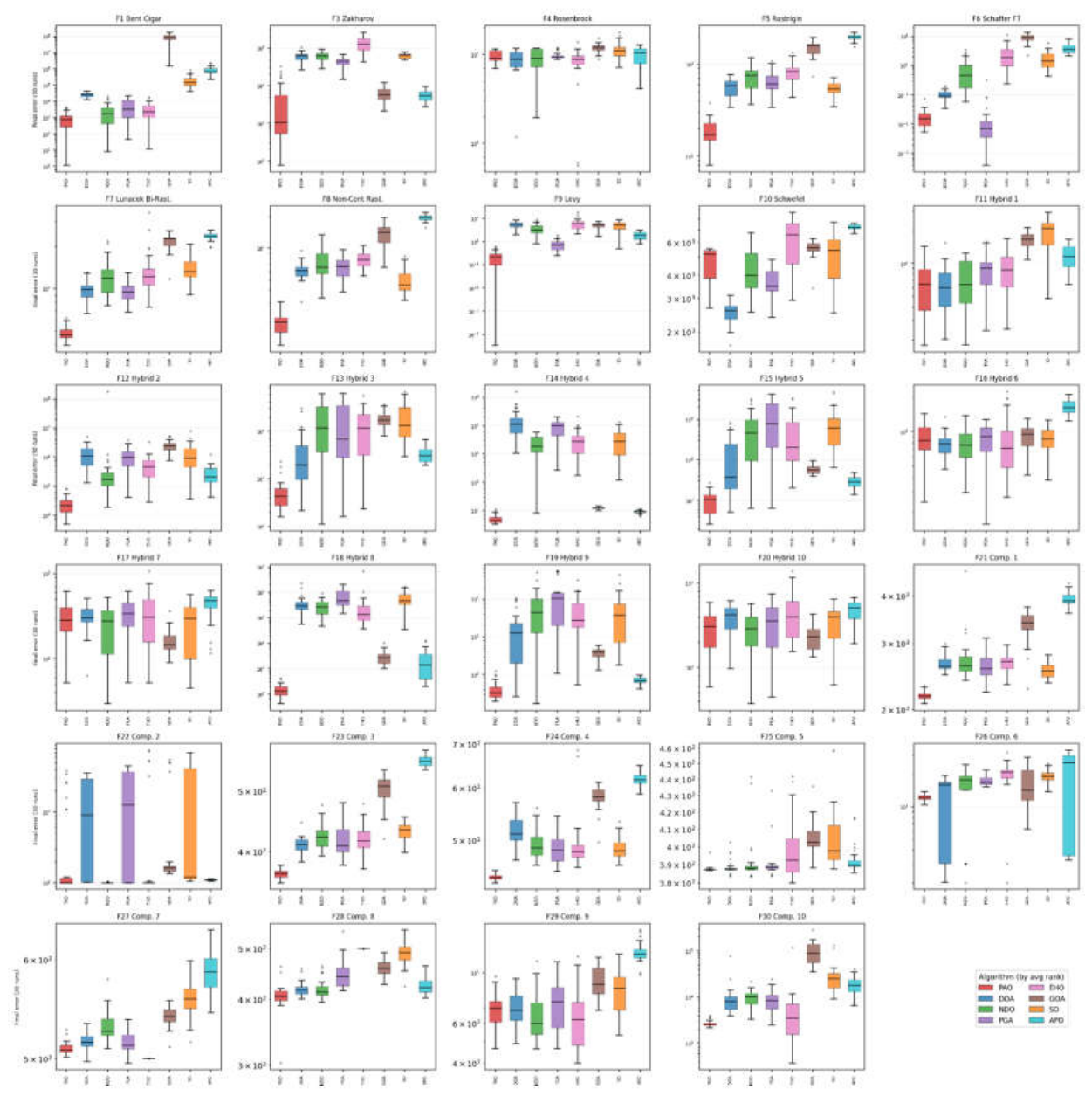
Figure 10.
Convergence behavior on the CEC-2019 “100-Digit Challenge” suite . Colors as in Figure 6.
Figure 10.
Convergence behavior on the CEC-2019 “100-Digit Challenge” suite . Colors as in Figure 6.
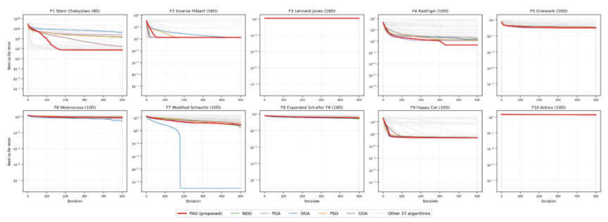
Figure 11.
Distribution of final errors on the CEC-2019 suite. PAO versus the eight leading optimizers by mean rank; lower is better and the axis is logarithmic (symmetric-log where values are non-positive).
Figure 11.
Distribution of final errors on the CEC-2019 suite. PAO versus the eight leading optimizers by mean rank; lower is better and the axis is logarithmic (symmetric-log where values are non-positive).
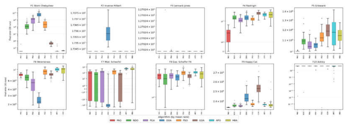
Figure 12.
Convergence behavior on the CEC-2022 benchmark suite (D = 10). Colors as in Figure 6.
Figure 12.
Convergence behavior on the CEC-2022 benchmark suite (D = 10). Colors as in Figure 6.
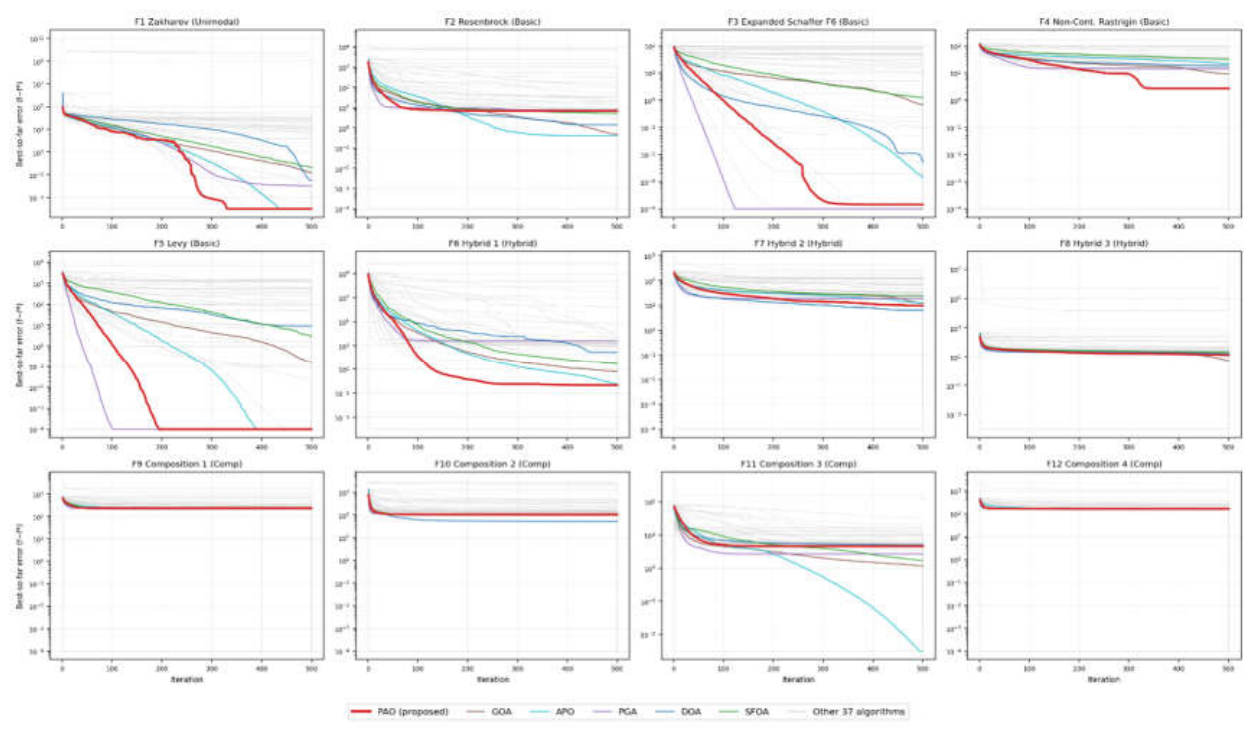
Figure 13.
Distribution of final errors on the CEC-2022 suite (D = 10). Conventions as in Figure 7.
Figure 13.
Distribution of final errors on the CEC-2022 suite (D = 10). Conventions as in Figure 7.
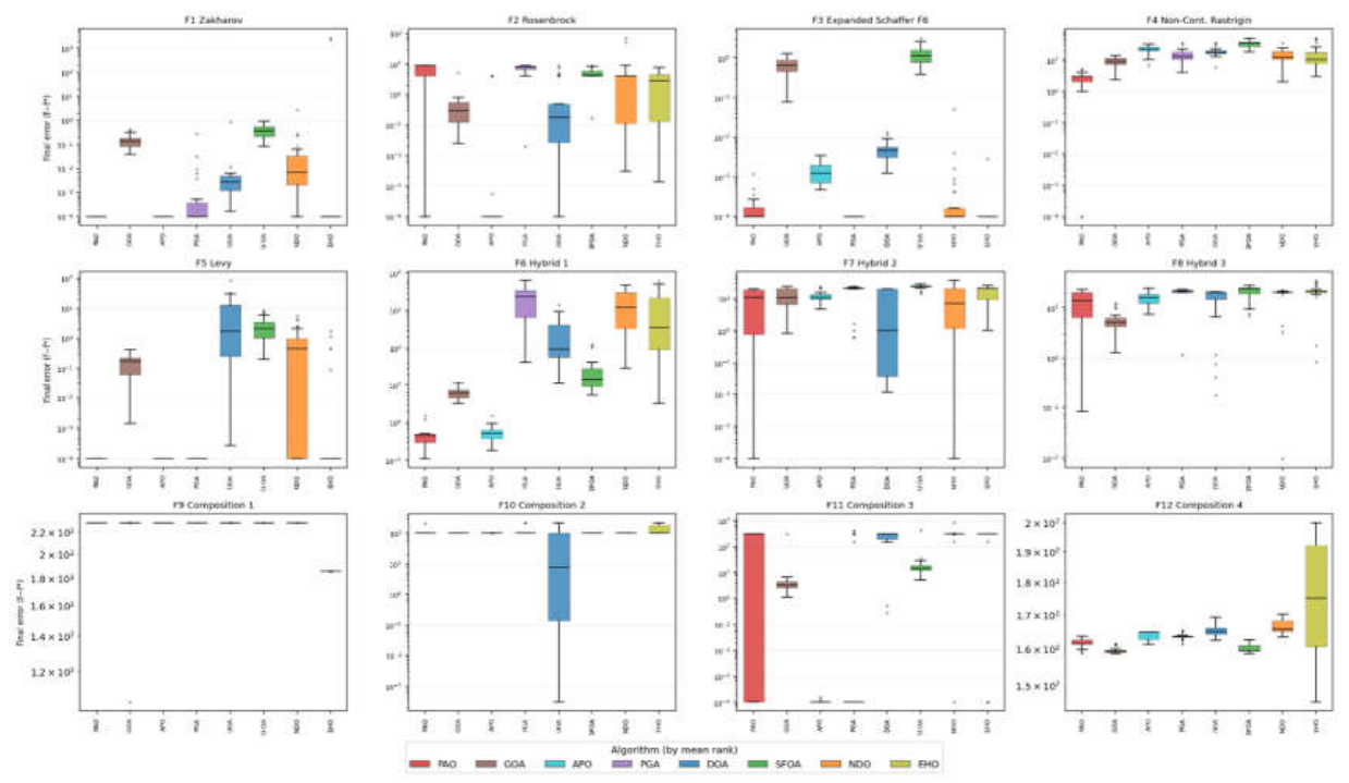
Figure 14.
Five-panel qualitative analysis of PAO on the unimodal function F1 (Sphere, 2-D): (a) landscape, (b) search history of all agents, (c) trajectory of the first agent’s first coordinate, (d) population-average fitness, (e) convergence. The visited points concentrate near the optimum and the trajectory damps quickly — the signature of exploitation-dominated search.
Figure 14.
Five-panel qualitative analysis of PAO on the unimodal function F1 (Sphere, 2-D): (a) landscape, (b) search history of all agents, (c) trajectory of the first agent’s first coordinate, (d) population-average fitness, (e) convergence. The visited points concentrate near the optimum and the trajectory damps quickly — the signature of exploitation-dominated search.
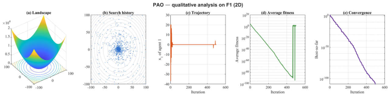
Figure 15.
Five-panel qualitative analysis of PAO on a multimodal function (F9, 2-D). Compared with the unimodal case, the search history samples several basins before contracting, and the trajectory sustains larger excursions for longer before settling — evidence of the additional exploration the landscape demands.
Figure 15.
Five-panel qualitative analysis of PAO on a multimodal function (F9, 2-D). Compared with the unimodal case, the search history samples several basins before contracting, and the trajectory sustains larger excursions for longer before settling — evidence of the additional exploration the landscape demands.
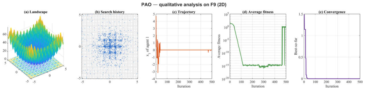
Figure 16.
Exploration versus exploitation for PAO on five classical benchmark functions. Bars show PAO’s run-averaged exploration (blue) and exploitation (red) percentages; black diamonds mark the mean exploration across all 43 algorithms on each function. PAO is exploitation-heavy on the unimodal and fixed-dimension functions but shifts to a balanced, exploration-heavy regime on the deceptive Schwefel function (F8).
Figure 16.
Exploration versus exploitation for PAO on five classical benchmark functions. Bars show PAO’s run-averaged exploration (blue) and exploitation (red) percentages; black diamonds mark the mean exploration across all 43 algorithms on each function. PAO is exploitation-heavy on the unimodal and fixed-dimension functions but shifts to a balanced, exploration-heavy regime on the deceptive Schwefel function (F8).
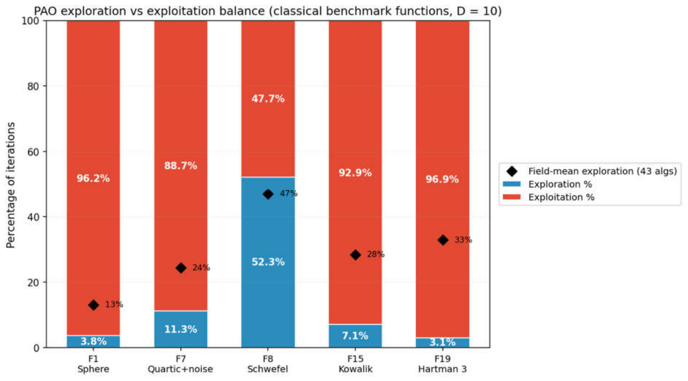
Figure 17.
Critical-difference diagrams for the four benchmark suites (Bonferroni–Dunn post-hoc, PAO as control, α = 0.05). PAO and the eleven next-best algorithms are placed on the average-rank axis; the red bar has length CD anchored at PAO, and algorithms lying beyond it are significantly worse. The wide CD values reflect the conservatism of a 43-way comparison.
Figure 17.
Critical-difference diagrams for the four benchmark suites (Bonferroni–Dunn post-hoc, PAO as control, α = 0.05). PAO and the eleven next-best algorithms are placed on the average-rank axis; the red bar has length CD anchored at PAO, and algorithms lying beyond it are significantly worse. The wide CD values reflect the conservatism of a 43-way comparison.
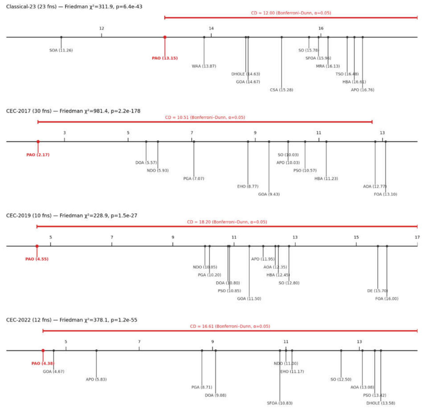
Figure 18.
Scalability of PAO across dimensions on the classical suite. (a) Mean solution error against D for F1–F13 (F8 omitted because its optimum scales with D); precision is progressively lost but the absolute errors stay moderate. (b) Mean runtime per run against D, with a linear-in-D reference: PAO’s cost grows only 1.33-fold from D = 10 to D = 100.
Figure 18.
Scalability of PAO across dimensions on the classical suite. (a) Mean solution error against D for F1–F13 (F8 omitted because its optimum scales with D); precision is progressively lost but the absolute errors stay moderate. (b) Mean runtime per run against D, with a linear-in-D reference: PAO’s cost grows only 1.33-fold from D = 10 to D = 100.
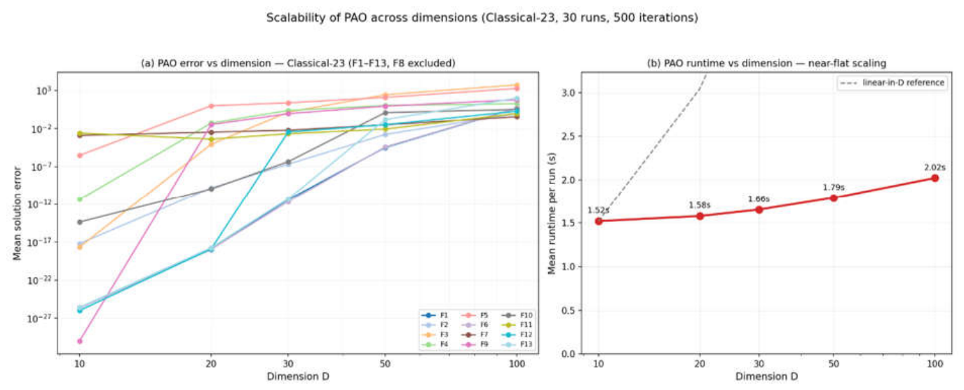
Figure 19.
Population-size sensitivity of PAO on the CEC-2019 suite. (a) Mean solution error against N for each of the ten functions (log–log axes); the error falls as N grows, most steeply on the hardest functions. (b) Average rank across the ten functions against N (lower is better) — the ordering is strictly monotone and N = 60 is best.
Figure 19.
Population-size sensitivity of PAO on the CEC-2019 suite. (a) Mean solution error against N for each of the ten functions (log–log axes); the error falls as N grows, most steeply on the hardest functions. (b) Average rank across the ten functions against N (lower is better) — the ordering is strictly monotone and N = 60 is best.
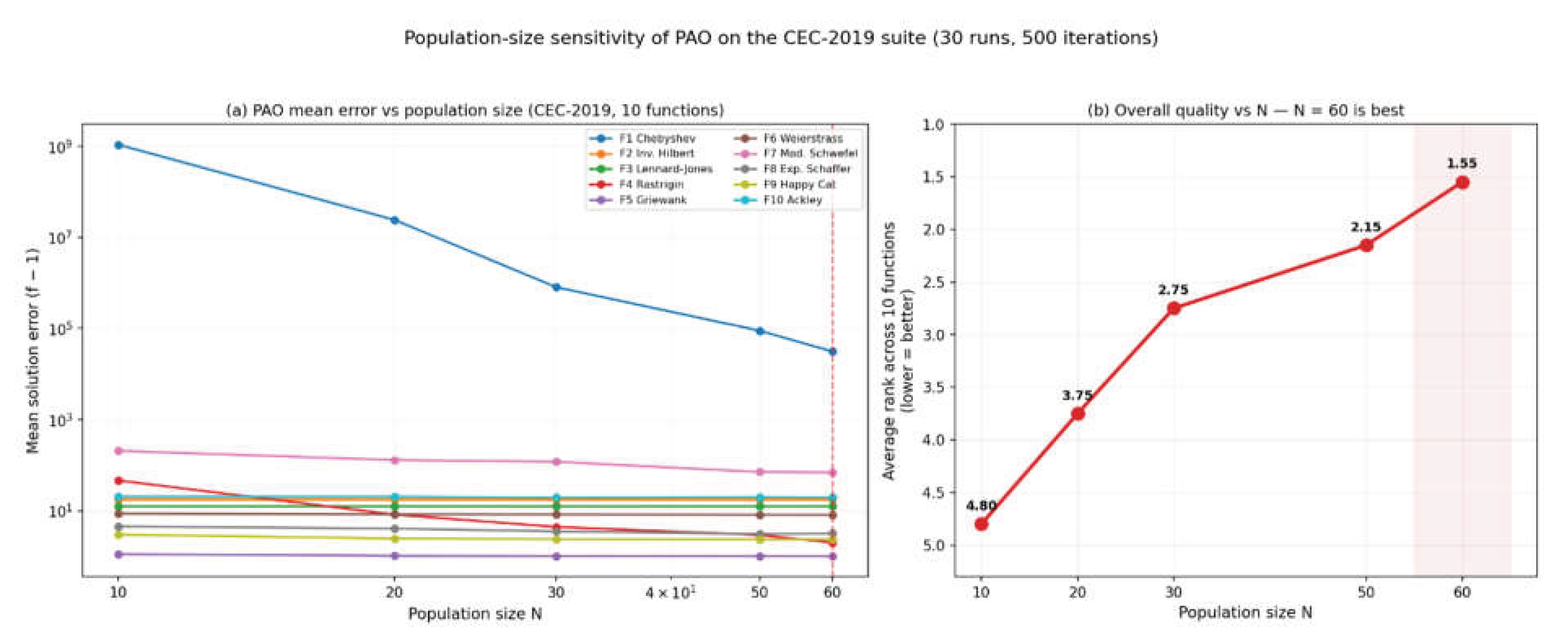
Figure 20.
Runtime analysis. (a) PAO’s mean runtime per run against the field median on each suite, annotated with its speed rank. (b) Speed rank versus accuracy rank on CEC-2017 for all 43 algorithms: the fastest methods (HS, DAOA, CSA) occupy the low-accuracy region while PAO attains the best accuracy at a high time cost.
Figure 20.
Runtime analysis. (a) PAO’s mean runtime per run against the field median on each suite, annotated with its speed rank. (b) Speed rank versus accuracy rank on CEC-2017 for all 43 algorithms: the fastest methods (HS, DAOA, CSA) occupy the low-accuracy region while PAO attains the best accuracy at a high time cost.
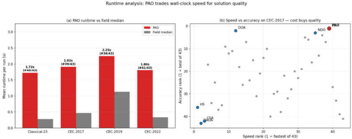
Figure 21.
Mean measured time complexity (T₂ − T₁)/T₀ over the 23 classical benchmark functions for all algorithms with a valid measurement, sorted from lightest to heaviest. PAO (red) ranks 34th of 40, between APO and CPO.
Figure 21.
Mean measured time complexity (T₂ − T₁)/T₀ over the 23 classical benchmark functions for all algorithms with a valid measurement, sorted from lightest to heaviest. PAO (red) ranks 34th of 40, between APO and CPO.
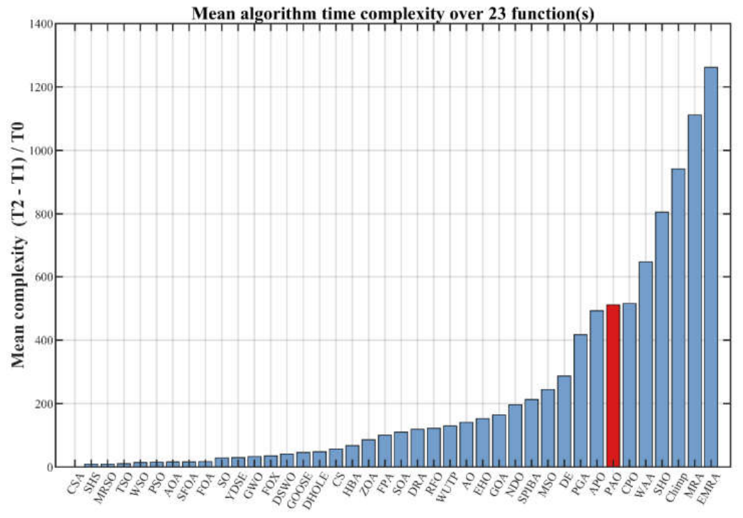
Figure 22.
(a) Measured complexity against the number of functions on which the full evaluation budget was consumed. Algorithms to the left of the dashed line, including the nominally lightest method CSA, are ranked on incomplete measurements; PAO is measured on all 23. (b) Asymptotic per-iteration work against population size: the log N term unique to PAO is an additive overhead of about 19% at N = 60 and shrinks in relative terms as the dimension grows.
Figure 22.
(a) Measured complexity against the number of functions on which the full evaluation budget was consumed. Algorithms to the left of the dashed line, including the nominally lightest method CSA, are ranked on incomplete measurements; PAO is measured on all 23. (b) Asymptotic per-iteration work against population size: the log N term unique to PAO is an additive overhead of about 19% at N = 60 and shrinks in relative terms as the dimension grows.
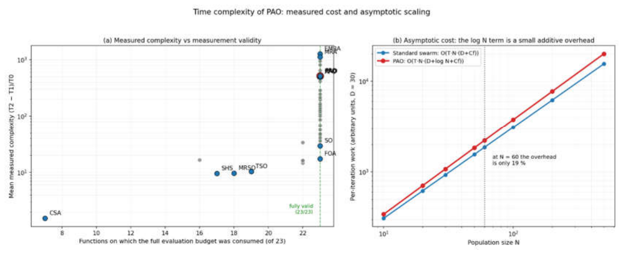
Figure 23.
Ablation of PAO on CEC-2017 (29 functions, 30 runs). (a) Wilcoxon outcome for each variant against the full algorithm: the five prayer-time operators (shaded) produce almost only ties, whereas the schedule ablations produce genuine disagreement in both directions. (b) Median versus mean change in error: the near-zero medians alongside large positive means show that the schedule ablations are typically harmless but occasionally catastrophic.
Figure 23.
Ablation of PAO on CEC-2017 (29 functions, 30 runs). (a) Wilcoxon outcome for each variant against the full algorithm: the five prayer-time operators (shaded) produce almost only ties, whereas the schedule ablations produce genuine disagreement in both directions. (b) Median versus mean change in error: the near-zero medians alongside large positive means show that the schedule ablations are typically harmless but occasionally catastrophic.
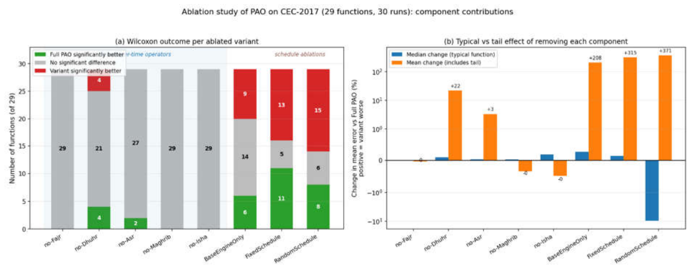
Figure 24.
Mean percentage degradation caused by removing each component (positive = removing it hurts). Only the schedule-level ablations register a substantial effect; the five prayer-time operators sit at or below zero, and randomizing the schedule improves the mean-percentage measure because that statistic is dominated by the typical case rather than the tail.
Figure 24.
Mean percentage degradation caused by removing each component (positive = removing it hurts). Only the schedule-level ablations register a substantial effect; the five prayer-time operators sit at or below zero, and randomizing the schedule improves the mean-percentage measure because that statistic is dominated by the typical case rather than the tail.
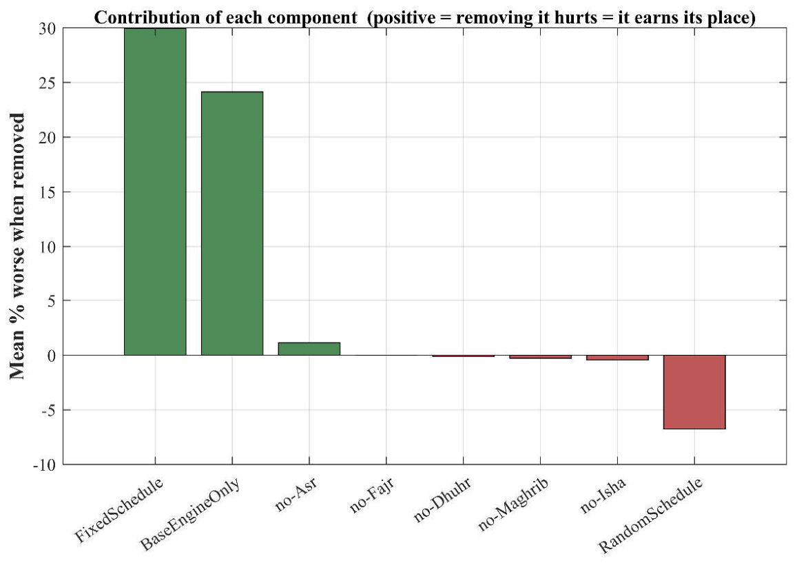
Table 2.
Metaheuristic algorithms reviewed in this study. For each algorithm the table gives its abbreviation, full name, year of introduction, number of citations reported by Google Scholar, and the original reference.
Table 2.
Metaheuristic algorithms reviewed in this study. For each algorithm the table gives its abbreviation, full name, year of introduction, number of citations reported by Google Scholar, and the original reference.
| No. | Algorithm | Algorithm full Name | Year |
No. of citation (Google Scholar) |
Reference |
|
PSO | Particle swarm optimization | 1995 | 97107 | (Kennedy & Eberhart, 1995) |
|
CS | Cuckoo search | 2009 | 9909 | (Yang & Deb, 2009) |
|
HS | Harmony Search | 2001 | 831 | (Zong Woo Geem et al., 2001) |
|
FPA | Flower Pollination Algorithm | 2012 | 3339 | (Yang, 2012) |
|
DE | Differential Evolution | 2013 | 1754 | (Price, 2013) |
|
GWO | Grey wolf optimizer | 2014 | 23733 | (Mirjalili et al., 2014) |
|
SHO | Spotted hyena optimizer | 2017 | 1187 | (Dhiman & Kumar, 2017) |
|
Chimp | Chimp optimization algorithm | 2020 | 1474 | (Khishe & Mosavi, 2020) |
|
TSO | Transient search optimization | 2020 | 243 | (Qais et al., 2020) |
|
AO | Aquila Optimizer | 2021 | 2685 | (Abualigah et al., 2021) |
|
AOA | Archimedes optimization algorithm | 2021 | 1428 | (Hashim et al., 2021) |
|
HBA | Honey Badger Algorithm | 2022 | 1510 | (Hashim et al., 2022) |
|
SO | Snake Optimizer | 2022 | 1383 | (Hashim & Hussien, 2022) |
|
ZOA | Zebra Optimization Algorithm | 2022 | 746 | (Trojovská et al., 2022) |
|
WSO | War Strategy Optimization | 2022 | 529 | (Ayyarao et al., 2022) |
|
DAOA | Dynamic Arithmetic Optimization Algorithm | 2022 | 165 | (Khodadadi et al., 2022) |
|
CSA | Circle Search Algorithm | 2022 | 127 | (Qais et al., 2022) |
|
MRA | Mud Ring Algorithm | 2022 | 78 | (Desuky et al., 2022) |
|
GOA | Gazelle optimization algorithm | 2023 | 621 | (Agushaka et al., 2023) |
|
FOX | FOX | 2023 | 329 | (H. Mohammed & Rashid, 2023) |
|
YDSE | Young’s double-slit experiment | 2023 | 209 | (Abdel-Basset et al., 2023) |
|
SOA | Skill Optimization Algorithm | 2023 | 142 | (Givi & Hubalovska, 2023) |
|
SFOA | Starfish optimization algorithm | 2025 | 401 | (Zhong et al., 2025) |
|
APO | Arctic puffin optimization | 2024 | 263 | (Wang et al., 2024) |
|
GOOSE | GOOSE | 2024 | 225 | (Hamad & Rashid, 2024) |
|
EHO | Elk herd optimizer | 2024 | 221 | (Al-Betar et al., 2024) |
|
FOA | Fossa Optimization Algorithm | 2024 | 93 | (Hamadneh et al., 2024) |
|
WAA | Weighted average algorithm | 2024 | 85 | (Cheng & De Waele, 2024) |
|
MRSO | Modified Rat Swarm Optimization | 2024 | 10 | (Abdulla et al., 2024) |
|
SHS | Scorpion Hunting Strategy | 2024 | 4 | (Singh et al., 2024) |
|
SPIBA | social psychology interaction behavior algorithm | 2024 | 2 | (Ameen, 2024) |
|
DOA | Dream Optimization Algorithm | 2025 | 201 | (Lang & Gao, 2025) |
|
CPO | Chinese Pangolin Optimizer | 2025 | 83 | (Guo et al., 2025) |
|
MSO | Mirage search optimization | 2025 | 60 | (He et al., 2025) |
|
DRA | Divine Religions Algorithm | 2025 | 54 | (Mozhdehi et al., 2025) |
|
PGA | Phototropic growth algorithm | 2025 | 49 | (Bohat et al., 2025) |
|
RFO | Rüppell’s fox optimizer | 2025 | 49 | (Braik & Al-Hiary, 2025b) |
|
DHOLE | Dhole optimization algorithm | 2025 | 46 | (B. O. Mohammed et al., 2025) |
|
WUTP | water uptake and transport in plants | 2025 | 28 | (Braik & Al-Hiary, 2025a) |
|
EMRA | Enhancement of the Mud Ring Algorithm | 2025 | 1 | (Ali & Ameen, 2025) |
|
NDO | Newton downhill optimizer | 2026 | 9 | (Xiao et al., 2026) |
|
DSWO | Dwarf Sperm Whale Optimization | 2026 | 0 | (J. Zhang, 2026) |
Table 3.
The five prayer times and the geometric condition that defines each. The depression angles used for Fajr and Isha vary slightly between calculation conventions; −18° and −17° are used throughout this study.
Table 3.
The five prayer times and the geometric condition that defines each. The depression angles used for Fajr and Isha vary slightly between calculation conventions; −18° and −17° are used throughout this study.
| Prayer | Geometric condition | Altitude used | Character of the interval |
| Fajr | first light; Sun a fixed depression below the horizon before sunrise | α = −18° | low Sun, long shadows, wide steps |
| Dhuhr | just after the Sun crosses the meridian | ω = 0 (plus a short offset) | highest Sun, shortest shadows |
| Asr | shadow has grown by k object-heights past its noon length | from Eq. (10) | shadows lengthening steadily |
| Maghrib | upper limb of the Sun touches the horizon | α = −0.833° | boundary event, short interval |
| Isha | twilight has disappeared after sunset | α = −17° | no Sun, longest interval |
Table 4.
The five phase windows in day angle, with the fraction of a run each occupies. The shares are properties of the windows alone and do not depend on latitude, season, or the number of iterations.
Table 4.
The five phase windows in day angle, with the fraction of a run each occupies. The shares are properties of the windows alone and do not depend on latitude, season, or the number of iterations.
| Phase | θ window | Share of the run | Operator applied | Primary role |
| Fajr | 340° – 360° | 5.1% | opposition re-seeding | exploration |
| (none) | 0° – 95° | 29.7% | base engine only | neutral |
| Dhuhr | 95° – 135° | 12.1% | median pull | balancing |
| Asr | 136° – 180° | 13.3% | Local Gaussian fine-tuning | exploitation |
| Maghrib | 181° – 200° | 4.8% | greedy attraction to best | exploitation |
| Isha | 201° – 339° | 35.1% | Lévy restart | exploration / recovery |
Table 5.
Validation of the day-angle windows against exact astronomical calculation for φ = 35°N on day 105, for which Eq. (1)–(7) give a declination of 9.41°, sunrise at 05:29 and sunset at 18:31. These are within a minute of the values hard-coded in the reference implementation, which confirms that its default clock corresponds to a real mid-latitude spring day.
Table 5.
Validation of the day-angle windows against exact astronomical calculation for φ = 35°N on day 105, for which Eq. (1)–(7) give a declination of 9.41°, sunrise at 05:29 and sunset at 18:31. These are within a minute of the values hard-coded in the reference implementation, which confirms that its default clock corresponds to a real mid-latitude spring day.
| Phase | window starts at θ | time from Eq. (8)–(9) | exact time from Eq. (6) | difference |
| Fajr | 340° | 04:16 | 04:00 | +16 min |
| Dhuhr | 95° | 12:22 | 12:03 | +19 min |
| Asr | 136° | 15:20 | 15:39 | −19 min |
| Maghrib | 181° | 18:34 | 18:31 | +4 min |
| Isha | 201° | 19:48 | 19:54 | −7 min |
Table 6.
Mapping from astronomy to algorithms. Each row pairs an astronomical quantity with the algorithmic quantity it determines and states the property the pairing contributes to the search — periodicity, unequal phase shares, or non-monotone ordering.
Table 6.
Mapping from astronomy to algorithms. Each row pairs an astronomical quantity with the algorithmic quantity it determines and states the property the pairing contributes to the search — periodicity, unequal phase shares, or non-monotone ordering.
| Astronomical quantity | Behavior over one day | Role inside PAO |
| solar altitude α, Eq. (3) | rises, peaks at noon, falls; not monotone | signal that orders the phases from exploration to exploitation and back |
| shadow ratio cot α, Eq. (5) | very large near sunrise and sunset, minimum at noon | natural profile for a search radius that recovers instead of decaying |
| sunrise and sunset, Eq. (7) | boundaries between day and night | anchors that fix θ = 0° and θ = 180° |
| latitude φ and day n, Eq. (1) | set the length of day and night | the only inputs to the schedule; a whole family of schedules at no tuning cost |
| the five prayer conditions, Table 3 | partition the cycle into five intervals of distinct geometry | the five operators of Section 3.6, Section 3.7, Section 3.8, Section 3.9 and Section 3.10 |
Table 7.
Nomenclature.
| Symbol | Meaning | Value or source |
| population size | user | |
| iteration budget | user | |
| d | problem dimension | problem |
| lb, ub | lower and upper bounds | problem |
| position of individual | — | |
| best solution found so far | — | |
| φ, n | latitude and day of year | schedule inputs |
| t, θ | clock time in minutes; day angle | Eq. (12), (8)–(9) |
| w | decay weight within the cycle | Eq. (13) |
| , | phase multipliers on the engine | Table 4 |
| MF, MCR | success-history memories, length | Eq. (22)–(23) |
| 𝒜 | external archive of replaced parents | capacity N |
| p | fraction of the population forming the set | 0.2 |
| Stagnation (no-improvement) counter of individual | reset on success |
Table 8.
Phase settings. multiplies the sampled scale factor and is added to the sampled crossover rate of the base engine (see section3.4).
Table 8.
Phase settings. multiplies the sampled scale factor and is added to the sampled crossover rate of the base engine (see section3.4).
| Phase | Extra operator | Strength coefficient | ||
| Fajr | 1.10 | −0.05 | opposition re-seeding of the worst 10% | none |
| Dhuhr | 0.95 | +0.05 | median pull on a random 30% | = 0.15 w |
| Asr | 0.90 | +0.05 | Local Gaussian refinement of a random 35% | = 0.25 w + 0.05 |
| Maghrib | 1.00 | +0.10 | greedy attraction of a random 30% | = 0.35 (1 − w) + 0.05 |
| Isha | 1.05 | −0.05 | Lévy restart of stagnated individuals | fixed scale 0.05 |
| (none) | 1.00 | 0.00 | none | — |
Table 9.
Role of each phase operator. The evaluation cost is additional to the N evaluations the base engine consumes every iteration.
Table 9.
Role of each phase operator. The evaluation cost is additional to the N evaluations the base engine consumes every iteration.
| Phase | Role | What it changes | Effect on diversity | Cost, evaluations |
| Fajr | exploration | mirrors the worst 10% through the box centre | increases | ⌈0.10N⌉ |
| (none) | neutral | nothing beyond the base engine | unchanged | 0 |
| Dhuhr | balancing | contracts 30% toward the population median | decreases mildly | ⌈0.30N⌉ |
| Asr | exploitation | Gaussian steps scaled by distance to x* | decreases | ⌈0.35N⌉ |
| Maghrib | exploitation | moves 30% toward x* | decreases strongly | ⌈0.30N⌉ |
| Isha | exploration | heavy-tailed jumps for stagnated individuals | increases | |S| ≥ ⌈0.05N⌉ |
Table 10.
Control parameters of PAO.
| Parameter | Default | Group | Role | Expected sensitivity |
| N, | user | universal | population and budget | high, as for any method |
| H | 10 | engine | memory length | low |
| p | 0.2 | engine | size of the set | moderate |
| |𝒜| | N | engine | archive capacity | low |
| 0.90–1.10 | PAO | phase multiplier on | moderate | |
| −0.05…+0.10 | PAO | phase offset on | moderate | |
| subset fractions (shares) | 0.10, 0.30, 0.35, 0.30 | PAO | how much of the population each operator touches | moderate |
| ηD, ηA, ηM | Table 8 | PAO | operator strength | high — the most sensitive group |
| β | 1.5 | PAO | Lévy index | low |
| Lévy scale | 0.05 | PAO | restart step size | moderate |
| max(15, 0.1·) | PAO | stagnation threshold | moderate | |
| φ, n | 35°N, day 105 | PAO | the schedule itself | to be measured — this is the novel axis |
Table 11.
PAO against four representative metaheuristics on the axes that define its contribution. Only PAO has a non-monotone control profile, a phase-structured multi-operator search, and a schedule that carries no fitted constant.
Table 11.
PAO against four representative metaheuristics on the axes that define its contribution. Only PAO has a non-monotone control profile, a phase-structured multi-operator search, and a schedule that carries no fitted constant.
| Algorithm | Control of the exploration–exploitation balance | Monotone? | Update structure | Schedule constant to tune? |
| PSO (Kennedy & Eberhart, 1995) | inertia weight driven down over the run | yes | one velocity rule applied to all particles | yes — inertia schedule, c₁, c₂ |
| DE (Storn & Price, 1997) | scale factor and crossover rate, optionally reduced over the run | yes (size) | one mutation-and-crossover rule throughout | search history, plus any size schedule |
| GWO (Mirjalili et al., 2014) | coefficient a decreased linearly from 2 to 0 | yes | one leader-following rule every iteration | yes — linear a |
| SCA (Mirjalili, 2016) | amplitude r₁ decreased linearly to 0 | yes | one sine–cosine rule applied throughout | yes — r₁ range and a |
| PAO (this work) | solar altitude and shadow ratio over one day | no | five phase operators plus a neutral gap, over an adaptive base engine | none in the schedule — fixed by φ and n |
Table 12.
Run-averaged exploration and exploitation percentages for PAO on five classical benchmark functions, with the mean exploration across all 43 algorithms for context. PAO explores far less than the field where exploitation is rewarded (F1, F7, F15, F19) yet matches or exceeds the field on the deceptive Schwefel function (F8).
Table 12.
Run-averaged exploration and exploitation percentages for PAO on five classical benchmark functions, with the mean exploration across all 43 algorithms for context. PAO explores far less than the field where exploitation is rewarded (F1, F7, F15, F19) yet matches or exceeds the field on the deceptive Schwefel function (F8).
| Fn | Function | PAO exploration % | PAO exploitation % | Field-mean exploration % |
| F1 | Sphere (unimodal) | 3.8 | 96.2 | 13.1 |
| F7 | Quartic + noise (unimodal) | 11.3 | 88.7 | 24.4 |
| F8 | Schwefel 2.26 (multimodal) | 52.3 | 47.7 | 47.0 |
| F15 | Kowalik (fixed-dimension) | 7.1 | 92.9 | 28.4 |
| F19 | Hartman 3 (fixed-dimension) | 3.1 | 96.9 | 32.9 |
Table 13.
Statistical summary across the four benchmark suites. Friedman overall statistics, PAO’s average rank and overall position, the aggregated Wilcoxon record for PAO against all 42 competitors, the Bonferroni–Dunn critical difference with PAO as control, and the number of algorithms PAO significantly outperforms under the Holm procedure.
Table 13.
Statistical summary across the four benchmark suites. Friedman overall statistics, PAO’s average rank and overall position, the aggregated Wilcoxon record for PAO against all 42 competitors, the Bonferroni–Dunn critical difference with PAO as control, and the number of algorithms PAO significantly outperforms under the Holm procedure.
| Suite | Fns | χ² | p-value | PAO avg rank | PAO position | Wilcoxon W/T/L | Win % | CD (BD) | Holm: PAO better than |
| Classical-23 | 23 | 311.91 | 6.35e-43 | 13.152 | 2 of 43 | 641/42/283 | 66.4 | 12.00 | 13 of 42 |
| CEC-2017 | 30 | 981.42 | 2.17e-178 | 2.167 | 1 of 43 | 1150/56/12 | 94.4 | 10.51 | 34 of 42 |
| CEC-2019 | 10 | 228.86 | 1.48e-27 | 4.550 | 1 of 43 | 362/31/27 | 86.2 | 18.20 | 19 of 42 |
| CEC-2022 | 12 | 378.08 | 1.24e-55 | 4.375 | 1 of 43 | 445/32/27 | 88.3 | 16.61 | 24 of 42 |
Table 14.
Scalability summary for PAO. Left: number of classical functions solved to a mean error below 10⁻⁸ at each dimension, and the mean runtime per run. Right: the same runtime expressed relative to D = 10.
Table 14.
Scalability summary for PAO. Left: number of classical functions solved to a mean error below 10⁻⁸ at each dimension, and the mean runtime per run. Right: the same runtime expressed relative to D = 10.
| Dimension D | Functions solved to < 10⁻⁸ | Mean runtime / run (s) | Runtime relative to D = 10 |
| D = 10 | 9 of 12 | 1.5222 | 1.00× |
| D = 20 | 6 of 12 | 1.5801 | 1.04× |
| D = 30 | 3 of 12 | 1.6553 | 1.09× |
| D = 50 | 0 of 12 | 1.7922 | 1.18× |
| D = 100 | 0 of 12 | 2.0225 | 1.33× |
Table 15.
Population-size sensitivity summary for PAO on CEC-2019. For each N: the average accuracy rank across the ten functions (1 = best), the number of functions on which that N gives the lowest mean error, and the average robustness (standard-deviation) rank. N = 60 is best on every criterion. Full per-function values are in Appendix H.
Table 15.
Population-size sensitivity summary for PAO on CEC-2019. For each N: the average accuracy rank across the ten functions (1 = best), the number of functions on which that N gives the lowest mean error, and the average robustness (standard-deviation) rank. N = 60 is best on every criterion. Full per-function values are in Appendix H.
| Population N | Avg accuracy rank | Functions with lowest error | Avg robustness rank |
| 10 | 4.80 | 1 of 10 | 4.50 |
| 20 | 3.75 | 1 of 10 | 3.20 |
| 30 | 2.75 | 1 of 10 | 2.80 |
| 50 | 2.15 | 1 of 10 | 2.55 |
| 60 | 1.55 | 6 of 10 | 1.95 |
Table 16.
Runtime summary for PAO across the four suites: mean wall-clock time per run, speed rank among the 43 algorithms (1 = fastest), the field median time, the fastest and slowest algorithms with their times, PAO’s accuracy position, and PAO’s cost per function evaluation.
Table 16.
Runtime summary for PAO across the four suites: mean wall-clock time per run, speed rank among the 43 algorithms (1 = fastest), the field median time, the fastest and slowest algorithms with their times, PAO’s accuracy position, and PAO’s cost per function evaluation.
| Suite | PAO time (s) | Speed rank | Field median (s) | Fastest algorithm (s) | Slowest algorithm (s) | PAO accuracy rank | µs / evaluation |
| Classical-23 | 1.7182 | 40 of 43 | 0.2799 | HS (0.0073) | EMRA (2.5176) | 2 of 43 | 57.3 |
| CEC-2017 | 1.9184 | 39 of 43 | 0.4688 | HS (0.0107) | MRA (6.5015) | 1 of 43 | 63.9 |
| CEC-2019 | 2.2482 | 36 of 43 | 1.1288 | HS (0.0244) | ZOA (42.8672) | 1 of 43 | 74.9 |
| CEC-2022 | 1.8046 | 41 of 43 | 0.3339 | HS (0.0087) | HBA (2.4435) | 1 of 43 | 60.2 |
Table 17.
Time complexity of PAO and representative competitors: theoretical complexity class, mean measured complexity (T₂ − T₁)/T₀ over the classical suite, the resulting rank among the 40 algorithms with valid measurements, and the number of functions on which the measurement was valid. PAO is the only algorithm whose theoretical class carries a log N term.
Table 17.
Time complexity of PAO and representative competitors: theoretical complexity class, mean measured complexity (T₂ − T₁)/T₀ over the classical suite, the resulting rank among the 40 algorithms with valid measurements, and the number of functions on which the measurement was valid. PAO is the only algorithm whose theoretical class carries a log N term.
| Rank | Algorithm | Theoretical complexity | Mean measured complexity | Valid functions (of 23) |
| 1 | CSA | O(T × N × (D + Cf)) | 1.55 | 7 |
| 6 | PSO | O(T × N × (D + Cf)) | 15.95 | 22 |
| 9 | FOA | O(T × N × (D + Cf)) | 17.31 | 23 |
| 10 | SO | O(T × N × (D + Cf)) | 29.40 | 23 |
| 12 | GWO | O(T × N × (D + Cf)) | 33.76 | 22 |
| 31 | DE | O(T × N × (D + Cf)) | 287.20 | 23 |
| 32 | PGA | O(T × N × (D + Cf)) | 417.40 | 23 |
| 33 | APO | O(T × N × (D + Cf)) | 492.64 | 23 |
| 34 | PAO | O(T × N × (D + log N + Cf)) | 511.68 | 23 |
| 35 | CPO | O(T × N × (D + Cf)) | 515.79 | 23 |
| 39 | MRA | O(T × N × (D + Cf)) | 1111.80 | 23 |
| 40 | EMRA | O(T × N × (D + Cf)) | 1261.98 | 23 |
Table 18.
Ablation summary on CEC-2017. For each variant: the component disabled, the Wilcoxon record against the full algorithm (W = full PAO significantly better, T = no significant difference, L = variant significantly better), the median and mean change in error relative to the full algorithm (positive = variant worse), and the resulting average rank and position among the nine configurations.
Table 18.
Ablation summary on CEC-2017. For each variant: the component disabled, the Wilcoxon record against the full algorithm (W = full PAO significantly better, T = no significant difference, L = variant significantly better), the median and mean change in error relative to the full algorithm (positive = variant worse), and the resulting average rank and position among the nine configurations.
| Variant | Component removed | W | T | L | Median Δ (%) | Mean Δ (%) | Avg rank | Position |
| Full PAO | nothing (baseline) | -- | -- | -- | 0.000 | 0.0 | 4.966 | 3.5 |
| no-Fajr | Fajr operator (Eq. 16) | 0 | 29 | 0 | 0.000 | 0.0 | 4.931 | 2 |
| no-Dhuhr | Dhuhr operator (Eq. 17) | 4 | 21 | 4 | +0.097 | +21.7 | 5.276 | 8.5 |
| no-Asr | Asr operator (Eq. 18) | 2 | 27 | 0 | +0.037 | +3.3 | 5.241 | 6.5 |
| no-Maghrib | Maghrib operator (Eq. 19) | 0 | 29 | 0 | +0.025 | -0.3 | 5.241 | 6.5 |
| no-Isha | Isha operator (Eq. 20) | 0 | 29 | 0 | +0.183 | -0.5 | 5.103 | 5 |
| BaseEngineOnly | All five operators + schedule | 6 | 14 | 9 | +0.266 | +208.2 | 5.276 | 8.5 |
| FixedSchedule | Solar schedule → fixed | 11 | 5 | 13 | +0.146 | +315.3 | 4.966 | 3.5 |
| RandomSchedule | Solar schedule → random | 8 | 6 | 15 | -9.738 | +371.2 | 4.000 | 1 |
Table 19.
The twenty-two constrained engineering design problems: dimension, number of inequality constraints, domain, the reference optimum from the literature, the best design found by PAO over 30 runs at N = 60, and PAO’s rank among the 43 algorithms. “Field best” indicates that no algorithm in the pool found a better design. The corrugated bulkhead problem (P10) of the original collection is excluded.
Table 19.
The twenty-two constrained engineering design problems: dimension, number of inequality constraints, domain, the reference optimum from the literature, the best design found by PAO over 30 runs at N = 60, and PAO’s rank among the 43 algorithms. “Field best” indicates that no algorithm in the pool found a better design. The corrugated bulkhead problem (P10) of the original collection is excluded.
| # | Problem | d | g | Domain | Reference optimum | PAO best found | Field best | PAO rank |
| P01 | Speed reducer (gearbox) | 7 | 11 | Mechanical | 2994.42 | 2994.42 | ✓ | 3 |
| P02 | Tension/compression spring | 3 | 4 | Mechanical | 0.0126652 | 0.0126652 | ✓ | 3 |
| P03 | Pressure vessel | 4 | 4 | Structural | 6059.71 | 6059.71 | ✓ | 1.5 |
| P04 | Three-bar truss | 2 | 3 | Structural | 263.896 | 263.896 | ✓ | 1.5 |
| P05 | Gear train ratio | 4 | 0 | Mechanical | -1.0000 × 10⁻⁴ | 2.7009 × 10⁻¹² | ✓ | 5 |
| P06 | Cantilever beam | 5 | 1 | Structural | 1.33996 | 1.33996 | ✓ | 1 |
| P07 | I-beam deflection | 4 | 2 | Structural | 0.0130741 | 0.0130741 | ✓ | 7 |
| P08 | Tubular column | 2 | 6 | Structural | 26.4864 | 26.4864 | ✓ | 6.5 |
| P09 | Piston lever | 4 | 4 | Mechanical | 8.4127 | 8.4127 | ✓ | 8 |
| P11 | Car side impact | 11 | 10 | Automotive | 22.843 | 22.843 | ✓ | 1 |
| P12 | Welded beam | 4 | 7 | Structural | 1.72485 | 1.72485 | ✓ | 1 |
| P13 | Reinforced concrete beam | 3 | 2 | Civil | 359.208 | 359.208 | ✓ | 2 |
| P14 | Multi-disk clutch brake | 5 | 8 | Mechanical | 0.235242 | 0.313657 | ✓ | 4 |
| P15 | Rolling element bearing | 10 | 9 | Mechanical | -81859 | -82842.2 | ✓ | 4 |
| P16 | Belleville disc spring | 4 | 7 | Mechanical | 1.97968 | 1.97967 | ✓ | 1 |
| P17 | Hydrostatic thrust bearing | 4 | 7 | Mechanical | 1625.44 | 19505.3 | ✓ | 2 |
| P18 | Robot gripper | 7 | 7 | Robotics | 2.5287 | 4.32372 | – | 2 |
| P19 | Gas transmission compressor | 4 | 1 | Process | 2.9649 × 10⁶ | 2.2927 × 10⁶ | ✓ | 3.5 |
| P20 | Stepped cone pulley | 5 | 11 | Mechanical | 16.63 | 16.0882 | ✓ | 2 |
| P21 | Planetary gear train | 6 | 4 | Mechanical | 0.525 | 0.52325 | – | 4 |
| P22 | 10-bar planar truss (FEM) | 10 | 18 | Structural | 5060.85 | 5060.85 | ✓ | 1 |
| P23 | Heat exchanger (Himmelblau) | 8 | 6 | Process | 7049.25 | 7049.25 | ✓ | 1 |
Table 20.
Overall standing of the ten leading algorithms on the engineering suite: average rank across twenty-two problems, number of problems on which the algorithm attains rank 1, and its Wilcoxon record against PAO (W = PAO significantly better, T = no significant difference, L = competitor significantly better). Aggregate for PAO: 843 W / 34 T / 47 L (91.2%).
Table 20.
Overall standing of the ten leading algorithms on the engineering suite: average rank across twenty-two problems, number of problems on which the algorithm attains rank 1, and its Wilcoxon record against PAO (W = PAO significantly better, T = no significant difference, L = competitor significantly better). Aggregate for PAO: 843 W / 34 T / 47 L (91.2%).
| # | Algorithm | Average rank | Problems won | W | T | L |
| 1 | PAO | 2.955 | 6 | -- | -- | -- |
| 2 | APO | 4.455 | 4 | 12 | 1 | 9 |
| 3 | GOA | 6.841 | 0 | 19 | 1 | 2 |
| 4 | SFOA | 8.341 | 1 | 19 | 1 | 2 |
| 5 | PGA | 8.886 | 1 | 14 | 3 | 5 |
| 6 | DHOLE | 11.136 | 0 | 19 | 3 | 0 |
| 7 | RFO | 11.455 | 1 | 21 | 0 | 1 |
| 8 | NDO | 11.523 | 0 | 19 | 1 | 2 |
| 9 | YDSE | 12.068 | 0 | 20 | 1 | 1 |
| 10 | SO | 12.091 | 0 | 17 | 2 | 3 |
Table 21.
Summary of PAO’s performance across the five test collections. Mean rank is over the functions or problems of that collection; the Wilcoxon record is aggregated over all 42 competitors.
Table 21.
Summary of PAO’s performance across the five test collections. Mean rank is over the functions or problems of that collection; the Wilcoxon record is aggregated over all 42 competitors.
| Collection | Functions | PAO mean rank | Position | Friedman p | Wilcoxon W/T/L | Win % |
| Classical 23 | 23 | 13.152 | 2 of 43 | 6.4 × 10⁻⁴³ | 641 / 42 / 283 | 66.4 |
| CEC-2017 | 29 | 2.167 | 1 of 43 | 8.2 × 10⁻¹⁷² | 1150 / 56 / 12 | 94.4 |
| CEC-2019 | 10 | 4.550 | 1 of 43 | 1.5 × 10⁻²⁷ | 362 / 31 / 27 | 86.2 |
| CEC-2022 | 12 | 4.375 | 1 of 43 | 1.2 × 10⁻⁵⁵ | 445 / 32 / 27 | 88.3 |
| Engineering | 22 | 2.955 | 1 of 43 | 2.1 × 10⁻¹²⁵ | 843 / 34 / 47 | 91.2 |
Disclaimer/Publisher’s Note: The statements, opinions and data contained in all publications are solely those of the individual author(s) and contributor(s) and not of MDPI and/or the editor(s). MDPI and/or the editor(s) disclaim responsibility for any injury to people or property resulting from any ideas, methods, instructions or products referred to in the content. |
© 2026 by the authors. Licensee MDPI, Basel, Switzerland. This article is an open access article distributed under the terms and conditions of the Creative Commons Attribution (CC BY) license (http://creativecommons.org/licenses/by/4.0/).
Copyright: This open access article is published under a Creative Commons CC BY 4.0 license, which permit the free download, distribution, and reuse, provided that the author and preprint are cited in any reuse.