
Submitted:
01 September 2026
Posted:
02 September 2026
You are already at the latest version
Abstract
Seasonal crop classification is essential for agricultural monitoring in regions affected by flooding, cloud cover, and shifting planting calendars [1,2]. Recent crop-mapping studies show that spatial context and temporal phenology jointly improve deep learning classification [3,4], but the comparative behavior of 1D, 2D, and 3D convolutional neural network (CNN) architectures remains underexplored in tropical seasonal systems [5]. This study evaluates 1D, 2D, and 3D CNN models for seasonal land-cover and crop classification in Thailand’s Tha Chin River Basin using multi-temporal Sentinel-1 and Sentinel-2 data. Optical vegetation indices and radar backscatter features were aggregated into seasonal datacubes for cool, hot, and wet seasons, with temporal interpolation and smoothing applied to reduce cloud-related gaps. The models were compared across seasons, and incremental experiments assessed the influence of input timesteps and feature bands on classification performance. Results show architecture-dependent seasonal behavior rather than a single universally dominant model: 1D CNNs depend strongly on sufficient temporal-spectral information, 2D CNNs benefit from spatially coherent crop patterns, and 3D CNNs provide a more complete spatio-temporal representation across seasonal conditions. A modified 3D CNN with Day-of-Year growth-stage features further explores phenological normalization, although label reliability and planting-date uncertainty remain limiting factors. The findings position CNN dimensionality as a key design choice for seasonal crop mapping and provide a baseline for future hybrid CNN-RNN and transformer-based approaches in climate-impacted agricultural regions.
Keywords:
remote sensing
; convolutional neural network
; in-season crop classification
; feature extractors
; transfer learning
; feature extraction
; domain shift
1. Introduction
Climate change has increased the frequency and severity of agricultural disruptions, including floods, droughts, and irregular seasonal conditions [6,7,8]. These disruptions affect crop growth, planting schedules, and food-security planning, particularly in river-basin agricultural systems where farmers depend on seasonal climate regularity. Timely land-cover and crop-type information is therefore essential for agricultural monitoring, disaster response, yield estimation, and policy support.
Satellite Earth observation has become a central tool for crop monitoring because it provides repeated, spatially explicit observations over large agricultural areas. Sentinel-2 provides optical multispectral observations that are useful for vegetation monitoring, while Sentinel-1 synthetic aperture radar (SAR) offers complementary information that is less affected by cloud cover [7,9]. Combining optical and radar observations is especially relevant in tropical and monsoon-influenced environments, where optical data gaps can limit wet-season crop mapping.
Despite this potential, seasonal crop classification remains difficult. Many crop-mapping workflows rely on annual or complete-season observations, which limit their usefulness for in-season decision-making [10,11]. Crop calendars can also shift because of flooding, market conditions, delayed planting, and other climate-related disturbances. These shifts create a domain mismatch between expected crop phenology and the actual spectral-temporal signal observed by satellites. Models trained on fixed temporal profiles may therefore misclassify crops when planting or growth stages occur earlier or later than expected.[9,12,13,14,15]
Deep learning methods have been increasingly used to address the spatial, spectral, and temporal complexity of crop classification. One-dimensional CNNs can learn temporal-spectral patterns from sequential reflectance or index profiles. Two-dimensional CNNs can capture spatial structure, field texture, and local neighborhood patterns. Three-dimensional CNNs can process spatial and temporal dimensions jointly, making them suitable for multi-temporal image datacubes. Recent hybrid CNN-LSTM studies have also shown that combining spatial feature extraction with recurrent temporal modeling can produce highly accurate crop maps. For example, a recent Sentinel-2 crop-mapping study reported strong performance from 2D CNN-GRU architectures, reinforcing the importance of spatial context and temporal phenology in crop discrimination.
However, before introducing recurrent or transformer modules, it is important to understand how the dimensionality of CNN architectures itself affects seasonal crop classification. This is particularly important in Thailand’s agricultural systems, where seasonal cloud cover, heterogeneous crop patterns, and planting-date uncertainty complicate model design. A controlled comparison of 1D, 2D, and 3D CNNs under the same Sentinel-1/Sentinel-2 preprocessing pipeline can clarify when temporal-spectral, spatial-spectral, and spatio-temporal representations are most useful. This study evaluates 1D, 2D, and 3D CNN architectures for seasonal land-cover and crop classification in Thailand’s Tha Chin River Basin. The objectives are:
- To compare 1D, 2D, and 3D CNN architectures for seasonal crop and land-cover classification across cool, hot, and wet seasons.
- To evaluate how input timesteps and feature bands affect classification performance and early-season mapping potential.
- To assess a modified 3D CNN with Day-of-Year (DoY) growth-stage features as an experimental approach for phenological normalization.
- To examine the role of CNN feature extraction relative to classical machine-learning classification.
- The contribution of this paper is a seasonal CNN architecture benchmark for Thailand that isolates the effect of CNN input dimensionality under a shared multi-source satellite workflow
2. Materials and Methods
2.1. Study Area
The study area is the Tha Chin River Basin in central Thailand. The basin extends approximately from 13 degrees 21 minutes N to 15 degrees 26 minutes N and covers about 13,492 square kilometers. It includes agricultural areas across Uthai Thani, Chainat, Suphan Buri, Ang Thong, Kanchanaburi, Nakhon Pathom, and Samut Sakhon. The basin is a distributary system connected to the Chao Phraya River and contains diverse agricultural land uses, including paddy, cassava, maize, and sugarcane.
This region is suitable for seasonal crop-classification research because agricultural activity is strongly structured by seasonal water availability and climate conditions. Flooding, rainfall variability, and delayed planting can shift crop phenology and complicate fixed-calendar crop mapping. The study evaluates three seasonal windows: cool season, hot season, and wet season.
Figure 1.
Geographic Location of Area of Interest.
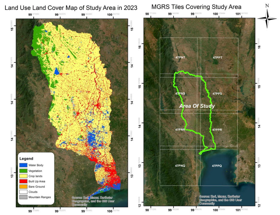
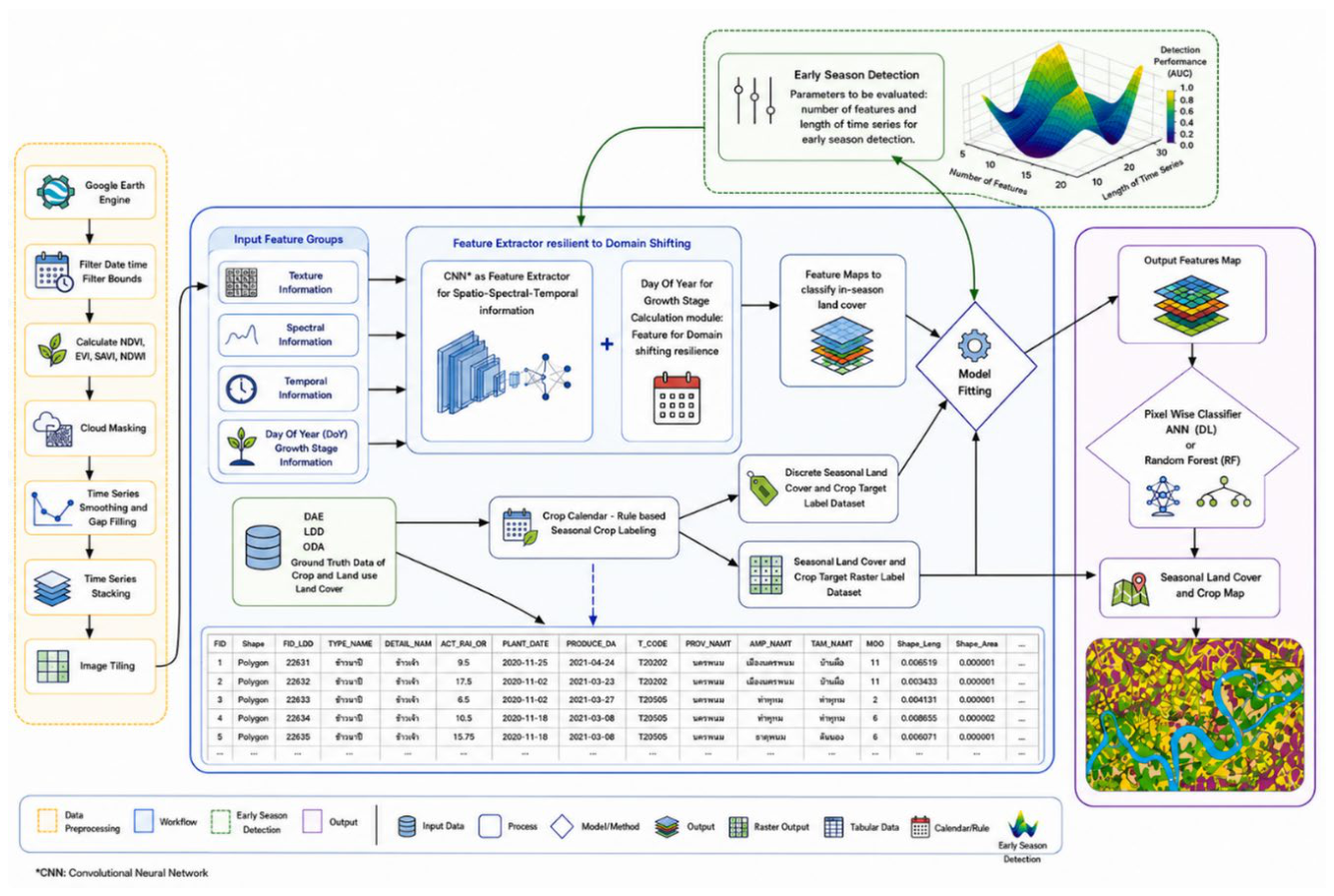
Figure 2.
Methodological workflow of this study.
2.2. Data Acquisition and Sources
This study used multi-source Earth observation and reference data to support seasonal crop classification in the Tha Chin River Basin, Thailand. The satellite data were acquired primarily from the European Space Agency Copernicus programme through the ESA Data Space/Catalog API. Sentinel-2 multispectral imagery was used to capture optical and vegetation-sensitive information, while Sentinel-1 Synthetic Aperture Radar imagery was used to provide complementary microwave backscatter observations that are less affected by cloud cover. The Sentinel-2 dataset included imagery from the relevant MGRS tiles covering the study area, with Level-1C and Level-2A products processed as needed for surface reflectance analysis. Sentinel-1 Ground Range Detected products were used in VV and VH polarizations, providing C-band radar observations across the seasonal windows.
The temporal design followed the agricultural seasonality of central Thailand. The research organized the analysis around cool, hot, and wet growing seasons, allowing crop separability to be evaluated under different phenological and environmental conditions. Optical and radar scenes were collected for each seasonal window, then organized into weekly time-series stacks. When multiple images were available within the same week, one representative scene was selected to maintain a regular temporal structure. This produced season-specific data cubes with shorter temporal depth for the hot season and longer temporal coverage for the cool and wet seasons.
Ground reference data were compiled from Thai agricultural and land-related agencies, including crop vector data with crop attributes and planting-date information. These reference data were combined with ancillary land-cover information to represent both agricultural and non-agricultural classes. The final classification scheme included major crop classes such as cassava, maize, paddy rice, and sugarcane, together with water, trees, built-up areas, and other or unknown crop areas. This design allowed the models to be evaluated not only on crop discrimination, but also on their ability to separate crops from spectrally or spatially competing land-cover classes.

Table 2.1.
Sentinel 2 Detail Information.
| Satellite Information | Sentinel-2 |
|---|---|
| Satellite name | Sentinel-2A / Sentinel-2B |
| Sensor Type | Optical multispectral sensor |
| Sensor Name | MSI — MultiSpectral Instrument |
| Temporal Resolution | 5 days |
| Spatial Resolution | 10 m, 20 m, and 60 m depending on spectral band |
Table 2.2.
Sentinel 1 Detail Information.
| Satellite Information | Sentinel-1 |
|---|---|
| Satellite name | Sentinel-1A / Sentinel-1C |
| Sensor Type | Active microwave radar sensor |
| Sensor Name | C-band Synthetic Aperture Radar |
| Temporal Resolution | 6 days with the constellation; 12 days per satellite |
| Spatial Resolution | 10 m GRD |
Ground-truth labels were derived from Thai agricultural and land-cover data sources, including crop-type data and land-cover classes. The target classification scheme includes seven classes:
Table 2.3.
Data Dictionary of Land cover and Crop Class.
| Value | Land Use and Land Cover Type |
|---|---|
| 1 | ‘Cassava’ |
| 2 | ‘Corn’ |
| 3 | ‘Paddy’ |
| 4 | ‘Sugarcane’ |
| 5 | ‘Water’ |
| 6 | ‘Trees’ |
| 11 | ‘Built Area’ |
The seasonal label preparation follows recorded planting-date information where available. Because some planting-date records are based on surveys or interviews, label timing may not always align with actual crop phenology. This is treated as an important limitation rather than hidden as noise.
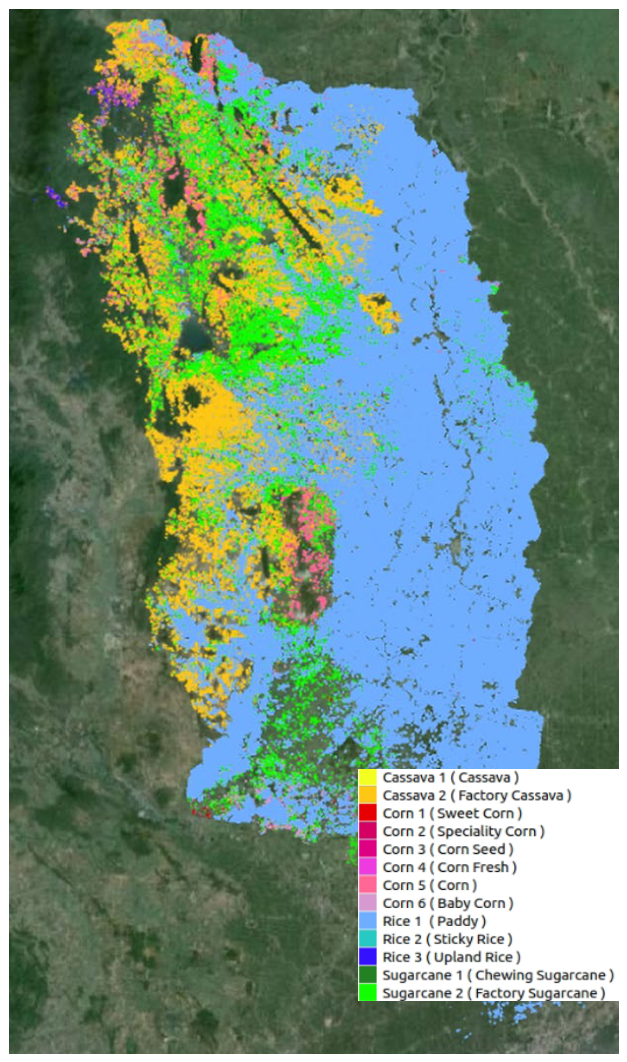
Figure 3.
Geographic Location of study area with Label data.
2.3. Feature Engineering and Label Preparation
Feature engineering was designed to combine spectral, radar, temporal, and phenological information in a common spatial framework. Sentinel-2 imagery was used to derive vegetation and water-sensitive indices, including NDVI, EVI, SAVI, and NDWI. Sentinel-1 imagery contributed VV and VH backscatter features, which were included to improve robustness under cloudy conditions and to capture structural differences among crop canopies. The optical vegetation-index time series were cloud masked, temporally interpolated where observations were missing, and smoothed using a Butterworth filter so that seasonal crop-growth patterns could be represented more consistently across the study area.
Four vegetation indices were calculated: NDVI, EVI, SAVI, and NDWI. These were combined with Sentinel-1 VV and VH bands to form spatio-temporal datacubes. Label data were split into three seasonal subsets based on government-recorded planting dates: Cool (Oct 14–Feb 14), Hot (Feb 14–May 14), and Wet (May 14–Oct 14). Two distinct training label datasets tailored to different modeling needs. The first dataset is designed for 1D Convolutional Neural Network (1DCNN) models, where the number of labels must match the number of labeled instances. This is achieved by directly tiling the dataset without any additional aggregation, ensuring a one-to-one correspondence between labels and data points.
Figure 4.
Seasonal Calendar Definition.

Figure 5.
Landcover and Crop label data preparation.
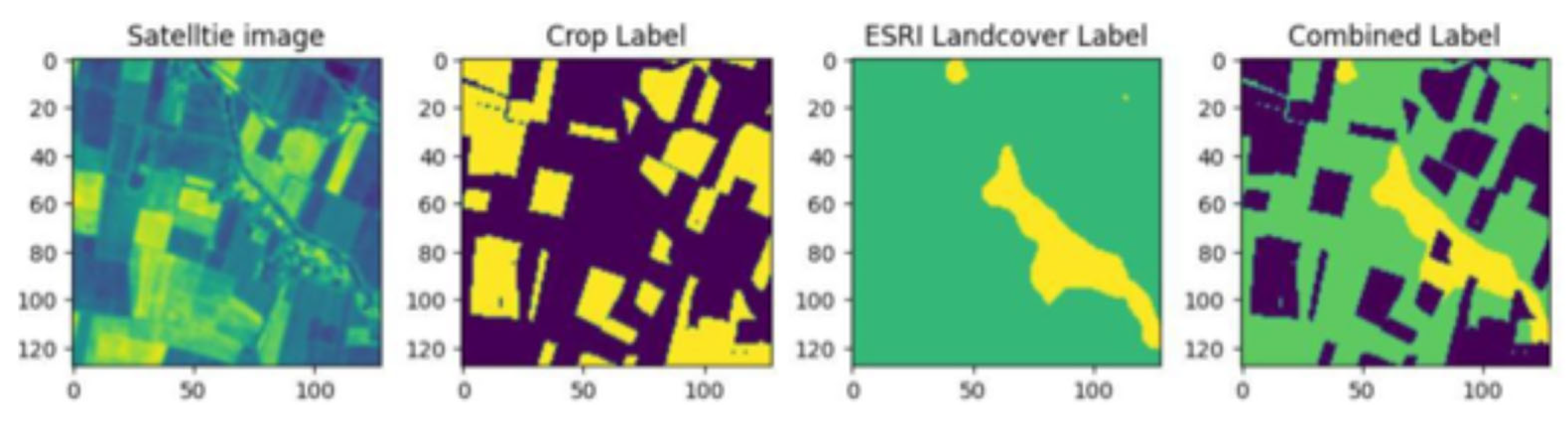
The second dataset is generated by transforming raster data into scalar values through majority-pixel value extraction within 8x8 raster tiles, employing a stride value of 1. Using a stride of 1 ensures that tiles overlap, maximizing the extraction of spatial information and increasing the number of representative samples available for classification. This method condenses the spatial data into a single scalar label for each tile, making it particularly well-suited for image-to-scalar value classification tasks where the goal is to associate each tile with a dominant land cover type.
Figure 6.
Label Data Preparation with Major Value for target label.
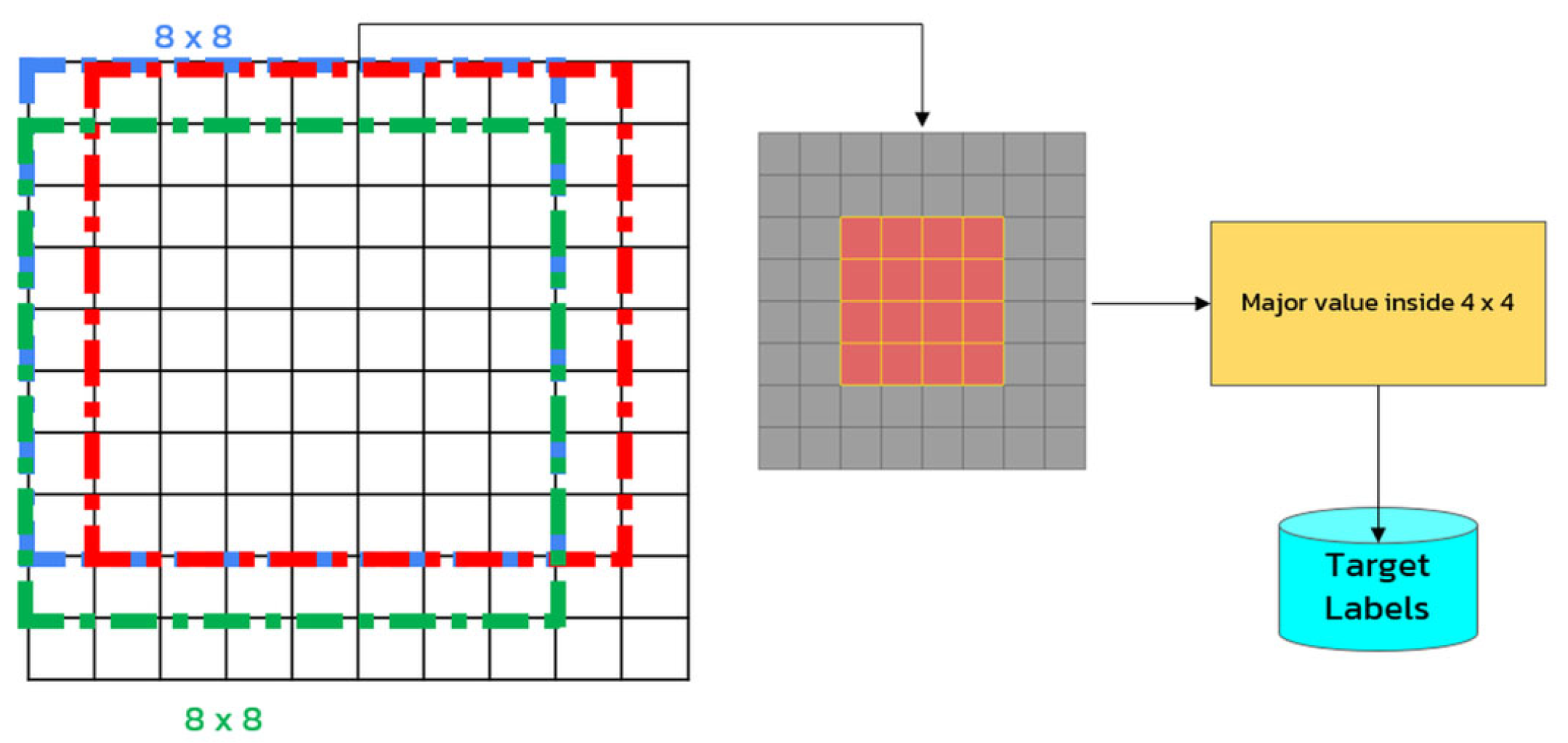
Table 2.4.
Description and calculating formulas for vegetational indices from Sentinel 2.
| Index | Abbreviation | Formula |
|---|---|---|
| NDVI | Normalized Difference Vegetation Index | |
| EVI | Enhanced Vegetation Index | |
| SAVI | Soil Adjusted Vegetation Index | |
| NDWI | Normalized Difference Water Index |
Table 2.5.
Description of Covariates from Sentinel 1.
| Index | Abbreviation | Formula |
|---|---|---|
| VV | Vertical-Vertical Polarization | |
| VH | Vertical-Horizontal Polarzation | |
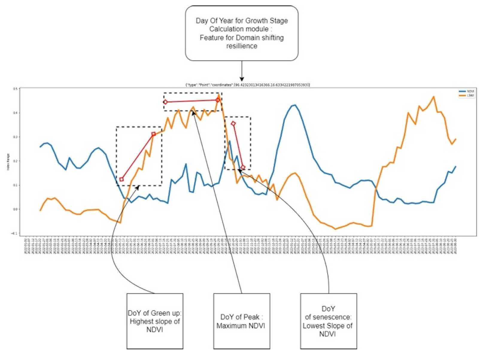
In addition to the main spectral and radar features, the study introduced day-of-year phenological descriptors derived from NDVI trajectories. These descriptors estimated key growth-stage timings, including green-up, peak growth, and senescence. The purpose of these variables was to provide the model with explicit seasonal timing information, helping distinguish crops that may appear similar in individual images but differ in their growth calendars. This phenological feature design was especially important for reframing the work as a seasonal crop-classification study rather than a static landcover classification task.
Figure 7.
Day of Year Calculation from NDVI time series.
2.4. Model Architectures and Training Protocol
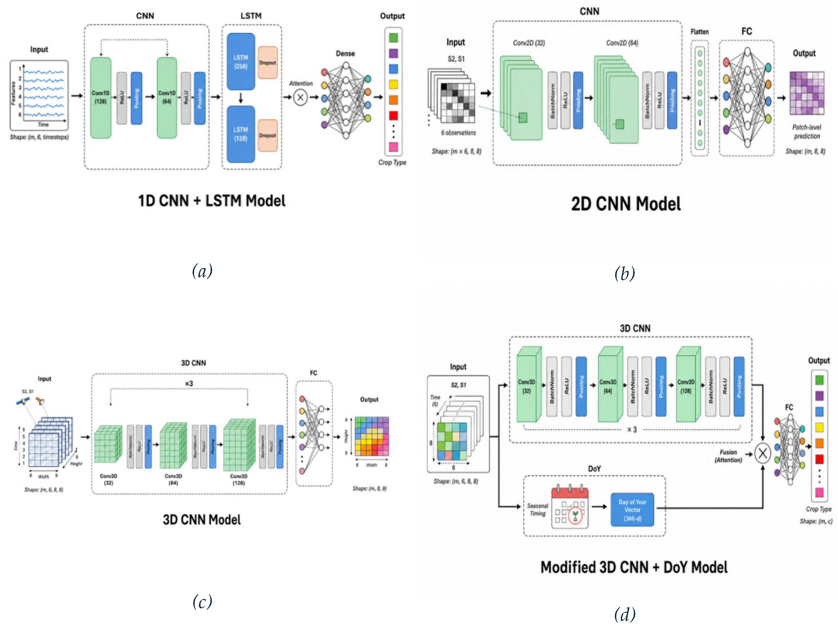
The research evaluated convolutional neural network architectures that differ in how they represent spectral, spatial, and temporal information. The one-dimensional CNN-based model served as a temporal-spectral baseline, focusing on feature variation through time while using a simplified spatial representation. The two-dimensional CNN treated stacked seasonal observations as multi-channel images, allowing the model to learn local spatial patterns while representing temporal information through the channel dimension. The three-dimensional CNN preserved time, feature, and spatial dimensions more explicitly, enabling convolutional filters to learn joint spatio-temporal patterns across the seasonal data cube. Four CNN-based architectures were developed using Python 3.10 and the PyTorch framework:
- 1DCNN-LSTM: Focused on temporal/spectral patterns from flattened spatial samples.
- 2DCNN: Leveraged spatial patterns within spectral bands across a flattened temporal dimension.
- 3DCNN: Simultaneously processed spatial, spectral, and temporal dimensions.
- Modified 3DCNN + DoY: Incorporated a Day of Year (DoY) module that calculated growth stages (greenup, peak, senescence) by analyzing NDVI slopes. These DoY vectors were concatenated with 3DCNN features before final classification
Figure 8.
Proposed four main architectures for seasonal crop classification: (a) 1D CNN approach (integrated with LST) that processes sequential feature vectors, and (b) 2DCNN approach designed for spatiotemporal patches (c) 3DCNN approach designed for Spatiotemporal Data cubes (d) 3DCNN +DoY modules designed for Spatiotemporal Data and Day of Year Vectors for each crop stages concatenated along with extracted features.
Figure 8.
Proposed four main architectures for seasonal crop classification: (a) 1D CNN approach (integrated with LST) that processes sequential feature vectors, and (b) 2DCNN approach designed for spatiotemporal patches (c) 3DCNN approach designed for Spatiotemporal Data cubes (d) 3DCNN +DoY modules designed for Spatiotemporal Data and Day of Year Vectors for each crop stages concatenated along with extracted features.
All models were implemented in Python using PyTorch. The preprocessing and data handling workflow used geospatial and scientific Python libraries including GDAL, Rasterio, NumPy, Pandas, GeoPandas, Shapely, scikit-learn, and matplotlib. The datasets were split into training and testing subsets using a 70:30 split. Models were trained with cross-entropy loss and the Adam optimizer, and softmax outputs were used for multiclass prediction. Training was conducted over multiple epochs, with the number of epochs adjusted according to model behavior and seasonal dataset performance.
Table 2.6.
Main hyperparameters and architectural components of proposed models emphasizing their differences.
Table 2.6.
Main hyperparameters and architectural components of proposed models emphasizing their differences.
| Component | 1D CNN-LSTM | 2D CNN | 3D CNN | 3D CNN+DoY |
|---|---|---|---|---|
| Input | 6 spectral-temporal features over 10 timesteps | Multi-channel 8 × 8 image patch | 6-channel image sequence over seasonal timesteps with 8 × 8 patches | 6-channel image sequence over seasonal timesteps with 8 × 8 patches |
| Convolution Layers | Conv1D: 16 , 32 | Conv2D: 32 , 32 , 64 | Conv3D: 32, 32, 64 | Conv3D: 32, 32, 64 |
| Kernel Size | 3 | 3 × 3 | 3 × 3 × 3 | 3 × 3 × 3 |
| Pooling | MaxPool1D | MaxPool2D (2, 2) | MaxPool3D (1, 2, 2) | MaxPool3D (1, 2, 2) |
| Normalization | Not Used | BatchNorm2D after each convolution | BatchNorm3D after each convolution | BatchNorm3D after each convolution |
| Dropout | Not Used | 0.1 after each convolution block | 0.1 after each convolution block | 0.1 after each convolution block |
| Temporal Modeling | LSTM with 128 units | Not used | Temporal dimension learned through 3D convolution | Temporal dimension learned through 3D convolution |
| Additional Features | None | None | None | Green-up, peak, and senescence features |
| Fully Connected Layers | 64 → 32 → Output | 64 → Output | 64 → Output | 64 → Output |
| Output Activation | Softmax | Softmax | Softmax | Softmax |
Model evaluation used standard classification metrics, including overall accuracy, precision, recall, F1-score, confusion matrices, and learning curves. Because the crop-reference data were imbalanced and some classes were represented by fewer samples, class-wise metrics were emphasized alongside overall accuracy. This was necessary because a model could achieve acceptable overall performance while still performing poorly on minority classes such as maize or on classes with strong spectral overlap such as cassava and sugarcane.
Models were trained with a 70/30 train-test split using the Adam optimizer and Cross Entropy loss. Incremental analysis was performed by systematically varying the number of input bands (1 to 6) and timesteps (seasonal lengths) to evaluate early-season mapping feasibility.
Model performance was evaluated using confusion matrices, classification reports, learning curves, and incremental input analysis. Because the classification task included multiple crop and land-cover classes with imbalanced sample distributions, overall accuracy was interpreted together with class-wise precision, recall, and F1-score. Confusion matrices were used to identify systematic misclassification between similar classes, particularly cassava and sugarcane, maize and other crop types, and built-up areas with mixed agricultural or vegetated pixels. Classification reports provided class-wise precision, recall, F1-score, and support, enabling the evaluation to distinguish between strong performance on dominant classes and balanced performance across all target categories.
Training and validation learning curves were used to assess convergence behavior, overfitting, and generalization across epochs. Decreasing training loss indicated successful model learning, while fluctuations in validation loss and validation accuracy were interpreted as evidence of possible overfitting, seasonal noise, or reduced generalization. Incremental analysis was additionally conducted by varying the number of input timesteps and feature bands. This analysis evaluated the sensitivity of each CNN architecture to seasonal data availability and assessed whether reliable classification could be achieved before the full seasonal time series was available. Together, these evaluation methods provided a comprehensive basis for comparing 1D, 2D, 3D, and modified 3D CNN architectures for seasonal crop classification.
Figure 9.
Confusion matrix for model evaluation.
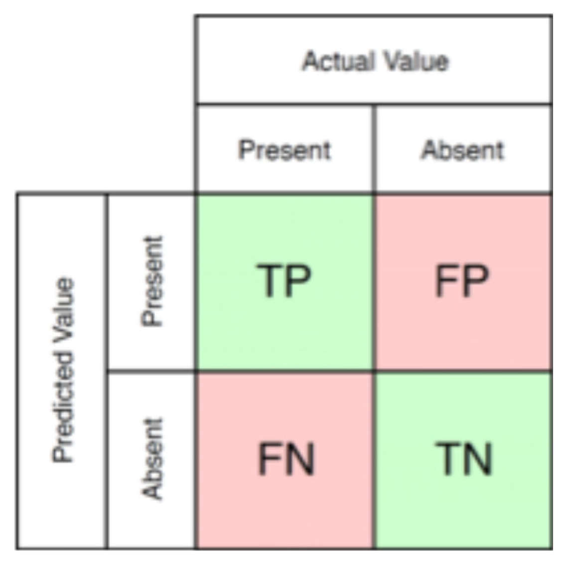
The metrics used for this multiclass classification model are accuracy, precision, recall and F1-Score. Multi class classification is a machine learning task that assigns the objects in the input data to one of several predefined categories. Therefore, the metrics used for these studies are accuracy, precision, recall and F1-Score. All the metrics being used in this study depend on true positive, true negative, false positive and false negative which are all used in classification tasks and help us understand how accurate our model is.
True positive is when the actual condition is present, and the model correctly identifies it as a present. True negative is when the actual condition is absent, and the model also correctly identifies it as an absent. False positive is when the actual condition is absent, and the model incorrectly identifies it as present. False negative is when the actual condition is present, and the model identifies it as absent.
The accuracy equation is the division of the sum of true positive and true negative by all the samples being predicted. It is one of the mainly used metrics yet the accuracy can be misleading when looking at single class at some point as it is also taking account on true negative, in other words, despite model poor performance in model identifying true positive, if a model able to identify the true negative, the accuracy will be likely to be higher than expected.
Precision is the division of true positive by the sum of true positive and false positive. Therefore, it is the measure of how often the model can make the correct predictions. The precision values range from 0 to 1 or as a percentage. The higher the precision, the better the model is.Recall is a metric that measures how often a model can correctly identify positive instances from all the actual positive samples in the dataset. Recall is the division of true positive by the addition of true positive and false negative. Recall values also range from 0 to 1 with 1 being the best.
Recall is a metric that measures how often a model can correctly identify positive instances from all the actual positive samples in the dataset. Recall is the division of true positive by the addition of true positive and false negative. Recall values also range from 0 to 1 with 1 being the best.
F1 score is the combination of recall and precision and therefore considers true positive, false positive and false negative and thus is a balanced idea of how good our model can perform. F1 Score ranges from 0 to 1 with 1 being the best.
3. Results
3.1. Overall Classification Performance Across Models and Seasons
Table 3.1.
Comparative overall accuracy (OA) of CNN Models.
| Model | Metric | Cool Season | Hot Season | Wet Season |
|---|---|---|---|---|
| 1D CNN | OA | 0.66 | 0.56 | 0.63 |
| 2D CNN | OA | 0.84 | 0.78 | 0.72 |
| 3D CNN | OA | 0.73 | 0.47 | 0.72 |
| 3D CNN + DoY | OA | 0.85 | 0.57 | 0.69 |
| Random forest | OA | 0.85 | 0.80 | 0.79 |
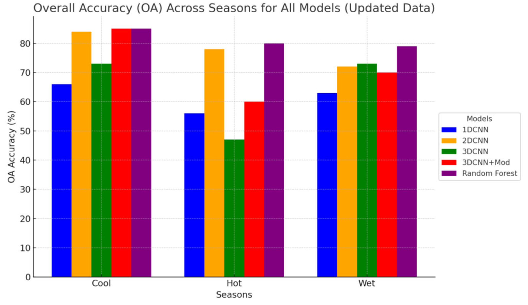
Table summarizes the overall classification performance of the evaluated models across the cool, hot, and wet seasons. The results demonstrate that model performance varied substantially across both architecture and season, indicating that no single CNN configuration was uniformly dominant under all seasonal conditions. The strongest CNN-based result was obtained by the modified 3D CNN with Day-of-Year (DoY) phenological features in the cool season, where it achieved an overall accuracy of 85% This performance was comparable to the Random Forest baseline in the same season, suggesting that explicit phenological descriptors can improve the separability of crop classes when seasonal growth signals are well expressed.
The 2D CNN showed the most consistent performance among the pure CNN models, achieving 84%, 78%, and 72% overall accuracy in the cool, hot, and wet seasons, respectively. This pattern suggests that spatial context from 8 x 8 image patches contributed substantially to crop and land-cover discrimination. The performance advantage of the 2D CNN over the 1D CNN is consistent with the interpretation that field structure, local texture, and neighborhood context are important for crop classification in heterogeneous agricultural landscapes.
The 1D CNN-LSTM model performed as a useful temporal-spectral baseline but showed lower overall accuracy than the 2D CNN in all seasons. Its performance reached 66% in the cool season, 56% in the hot season, and 63% in the wet season. These results indicate that temporal-spectral patterns alone were insufficient for robust classification across the study area, particularly where crop classes shared similar seasonal trajectories or where spatial context was needed to distinguish agricultural fields from built-up or tree-covered areas.
The standard 3D CNN achieved 73% accuracy in the cool season and 72% in the wet season, but dropped to 47% in the hot season. This result indicates that preserving the spatial-temporal structure of the datacube can be beneficial, but that 3D convolutional learning remains sensitive to seasonal data quality, label reliability, and crop separability. The hot-season result was the weakest among the main CNN outputs, suggesting that the shorter seasonal sequence and reduced phenological separation limited the ability of the 3D CNN to generalize.
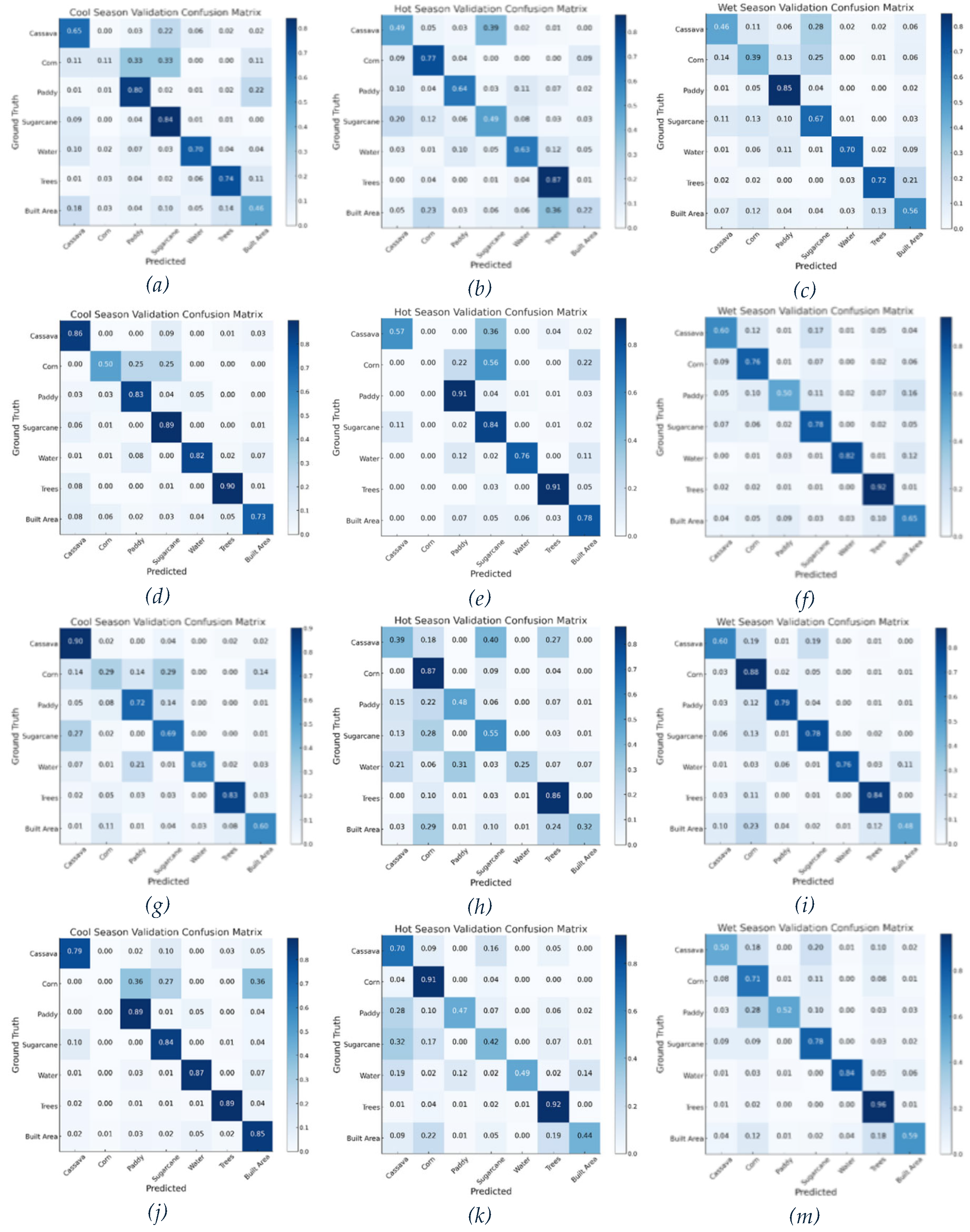
3.2. Class-Wise Accuracy Assessment and Confusion Matrix
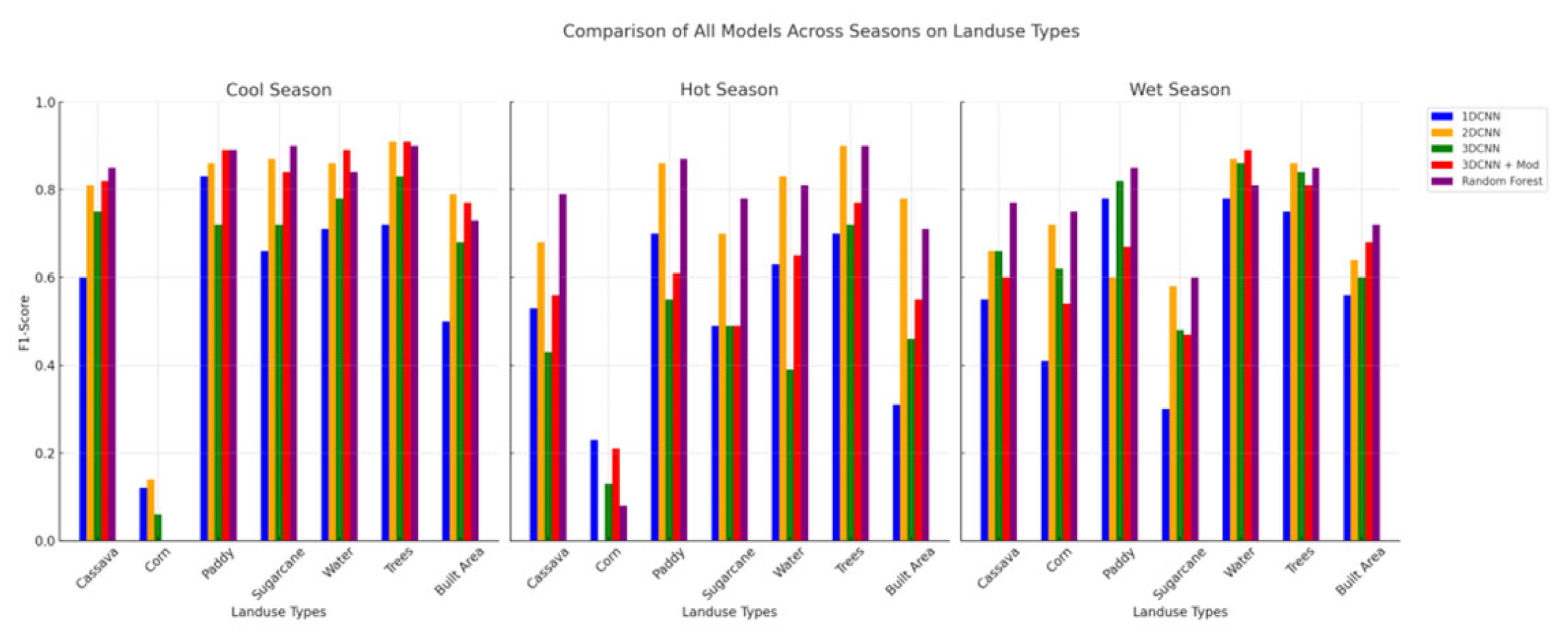
Class-wise evaluation shows that performance was uneven across crop and land-cover categories. Stable land-cover classes such as water and trees were generally classified more reliably than several crop classes. This pattern is expected because water and tree cover often exhibit more distinct spectral, radar, and spatial characteristics than seasonal crops. Paddy rice also achieved strong performance in several experiments, particularly where water-related and vegetation-growth signals made it separable from other crops.
The 2D CNN cool-season result showed strong class-level performance, with high F1-scores for trees, sugarcane, paddy rice, and water. The model achieved an overall accuracy of 84% and a weighted F1-score of 0.85, indicating balanced performance across the dominant classes. However, maize remained difficult because of limited representation and class confusion, with low precision despite moderate recall. Built-up areas also showed some confusion with trees and water, likely reflecting mixed pixels and heterogeneous peri-urban landscapes.
In the hot season, the 2D CNN achieved 78% overall accuracy and a weighted F1-score of 0.78. Trees, water, and paddy rice were classified strongly, while cassava and sugarcane showed higher confusion. Cassava reached moderate recall but was frequently misclassified as sugarcane, reflecting overlapping spectral or structural characteristics during this period. Maize remained one of the weakest classes, indicating that limited samples and seasonal ambiguity reduced class reliability.
For the wet season, the 2D CNN achieved 72% overall accuracy and a weighted F1-score of 0.72. Water and trees remained strong, while cassava and maize showed moderate improvement. Paddy and sugarcane were more difficult, partly because wet-season flooding and high moisture conditions can alter spectral and radar responses. These results show that wet-season classification is not only affected by cloud cover but also by changes in crop-water interactions and field conditions.
The 3D CNN class-wise results showed mixed behavior. In the cool season, cassava achieved high recall but lower precision, indicating that the model detected many cassava samples but also confused other classes as cassava. Paddy and sugarcane achieved moderate F1-scores, while maize remained weak. In the wet season, the 3D CNN improved substantially for paddy rice, trees, and water, with an overall accuracy of 72% and weighted F1-score of 0.73. However, sugarcane and built-up areas continued to show lower F1-scores, suggesting persistent class overlap.
The modified 3D CNN + DoY model produced its strongest class-wise behavior in the cool season. Paddy, trees, water, sugarcane, and cassava achieved strong F1-scores, while built-up areas showed moderate performance. Maize remained problematic, with very weak precision and recall. In the hot season, the modified model improved over the standard 3D CNN but still achieved only 57% overall accuracy, with maize showing high recall but very low precision. This indicates that the model frequently over-predicted maize, a pattern that should be discussed as a class-imbalance and label-reliability issue rather than as a successful maize result.
Overall, the confusion-matrix evidence indicates that classification errors were concentrated in crop classes with similar phenology, limited training representation, or mixed spatial context. Cassava-sugarcane confusion, maize instability, and built-up/vegetation mixing are the main recurring error patterns. This class-wise behavior is central to the paper’s findings because it shows that aggregate accuracy alone does not fully explain model performance.
Figure 10.
Confusion matrices for all four models at seasons (a) 1D CNN-LSTM Cool Season (b) 1D CNN-LSTM Hot Season (c) 1D CNN-LSTM Wet Season (d) 2D CNN Cool Season, (e) 2DCNN Hot Season (f) 2DCNN Wet Season (g) 3DCNN Cool Season (h) 3DCNN Hot Season (i) 3DCNN Wet Season (j) 3DCNN+DOY Cool Season (k) 3DCNN+DOY Hot Season (m) 3DCNN+DOY Wet Season.
Figure 10.
Confusion matrices for all four models at seasons (a) 1D CNN-LSTM Cool Season (b) 1D CNN-LSTM Hot Season (c) 1D CNN-LSTM Wet Season (d) 2D CNN Cool Season, (e) 2DCNN Hot Season (f) 2DCNN Wet Season (g) 3DCNN Cool Season (h) 3DCNN Hot Season (i) 3DCNN Wet Season (j) 3DCNN+DOY Cool Season (k) 3DCNN+DOY Hot Season (m) 3DCNN+DOY Wet Season.
3.3. Learning Curves and Convergence Behavior
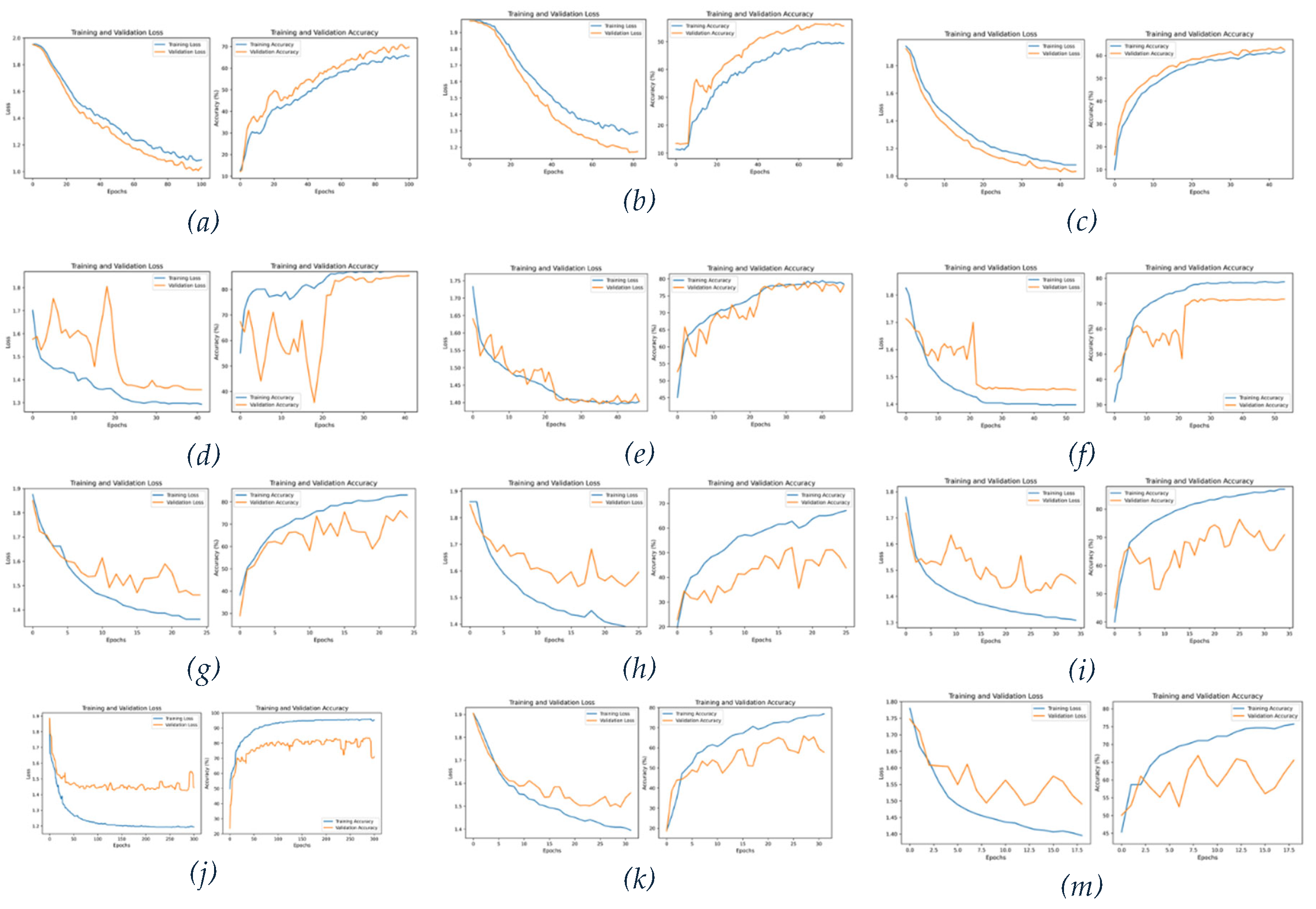
The learning curves provide additional insight into model generalization across seasons. For the 2D CNN, training loss decreased steadily across the seasonal experiments, indicating that the model learned useful representations from the input features. Validation accuracy stabilized near the final reported accuracy levels, particularly in the hot and wet seasons. However, fluctuations in validation loss were observed, suggesting that the model remained sensitive to seasonal variation, class imbalance, and validation-set composition.
The standard 3D CNN exhibited stronger seasonal dependence. In the cool season, training accuracy increased consistently and training loss decreased, while validation accuracy improved with some fluctuations. This indicates that the model learned spatial-temporal patterns but did not generalize perfectly to unseen validation samples. In the hot season, validation loss fluctuated more strongly and validation accuracy was less stable. This behavior aligns with the lower hot-season accuracy and suggests that the shorter temporal sequence and weaker phenological separability made the hot-season dataset harder for 3D convolutional learning.
The wet-season 3D CNN showed more stable learning than the hot-season case. Training loss decreased consistently, validation loss stabilized after early fluctuations, and training-validation divergence was limited. This suggests that, despite cloud and moisture-related challenges, the wet-season datacube contained stronger temporal structure for some classes, especially paddy, water, and trees.
The modified 3D CNN + DoY model showed the most stable convergence in the cool season. Training loss declined steadily, validation loss remained comparatively stable, and validation accuracy followed the training trend without severe divergence. This supports the interpretation that explicit phenological timing features can improve model learning when crop-growth calendars are reliable. In the hot and wet seasons, however, the modified model did not produce uniformly stronger performance, indicating that DoY features are sensitive to label timing, planting-date uncertainty, and seasonal noise.
Figure 11.
Training and Validation curves (a) training and validation accuracy curves 1D CNN-LSTM Cool Season (b) training and validation accuracy curves 1D CNN-LSTM Hot Season (c) training and validation accuracy curves 1D CNN-LSTM Wet Season (e) training and validation accuracy curves 2D CNN Cool Season (f) training and validation accuracy curves 2D CNN Hot Season (g) training and validation accuracy curves 2D CNN Wet Season (h) training and validation accuracy curves 3D CNN Cool Season (i) training and validation accuracy curves 3D CNN Hot Season (j) training and validation accuracy curves 3D CNN Wet Season (k) training and validation accuracy curves 3D CNN+DoY Cool Season (l) training and validation accuracy curves 3D CNN+DoY Hot Season (m) training and validation accuracy curves 3D CNN+DoY Wet Season.
Figure 11.
Training and Validation curves (a) training and validation accuracy curves 1D CNN-LSTM Cool Season (b) training and validation accuracy curves 1D CNN-LSTM Hot Season (c) training and validation accuracy curves 1D CNN-LSTM Wet Season (e) training and validation accuracy curves 2D CNN Cool Season (f) training and validation accuracy curves 2D CNN Hot Season (g) training and validation accuracy curves 2D CNN Wet Season (h) training and validation accuracy curves 3D CNN Cool Season (i) training and validation accuracy curves 3D CNN Hot Season (j) training and validation accuracy curves 3D CNN Wet Season (k) training and validation accuracy curves 3D CNN+DoY Cool Season (l) training and validation accuracy curves 3D CNN+DoY Hot Season (m) training and validation accuracy curves 3D CNN+DoY Wet Season.
3.4. Incremental Analysis of Timesteps and Features
The incremental analysis evaluated how classification accuracy changed as the number of input timesteps and feature bands increased. This analysis is important because operational crop mapping often requires early-season predictions before the full seasonal time series is available. It also helps identify whether performance gains arise from additional temporal observations, additional feature channels, or the model’s ability to exploit spatial-temporal structure.
Figure 12.
(a) Incremental Analysis of Timesteps and bands accuracy surface 1D CNN-LSTM Cool Season (b) Incremental Analysis of Timesteps and bands accuracy surface 1D CNN-LSTM Hot Season (c) Incremental Analysis of Timesteps and bands accuracy surface 1D CNN-LSTM Wet Season (e) Incremental Analysis of Timesteps and bands accuracy surface 2D CNN Cool Season (f) Incremental Analysis of Timesteps and bands accuracy surface 2D CNN Hot Season (g) Incremental Analysis of Timesteps and bands accuracy surface 2D CNN Wet Season (h) Incremental Analysis of Timesteps and bands accuracy surface 3D CNN Cool Season (i) Incremental Analysis of Timesteps and bands accuracy surface 3D CNN Hot Season (j) Incremental Analysis of Timesteps and bands accuracy surface 3D CNN Wet Season (k) Incremental Analysis of Timesteps and bands accuracy surface 3D CNN+DoY Cool Season (l) Incremental Analysis of Timesteps and bands accuracy surface 3D CNN+DoY Hot Season (m) Incremental Analysis of Timesteps and bands accuracy surface 3D CNN+DoY Wet Season.
Figure 12.
(a) Incremental Analysis of Timesteps and bands accuracy surface 1D CNN-LSTM Cool Season (b) Incremental Analysis of Timesteps and bands accuracy surface 1D CNN-LSTM Hot Season (c) Incremental Analysis of Timesteps and bands accuracy surface 1D CNN-LSTM Wet Season (e) Incremental Analysis of Timesteps and bands accuracy surface 2D CNN Cool Season (f) Incremental Analysis of Timesteps and bands accuracy surface 2D CNN Hot Season (g) Incremental Analysis of Timesteps and bands accuracy surface 2D CNN Wet Season (h) Incremental Analysis of Timesteps and bands accuracy surface 3D CNN Cool Season (i) Incremental Analysis of Timesteps and bands accuracy surface 3D CNN Hot Season (j) Incremental Analysis of Timesteps and bands accuracy surface 3D CNN Wet Season (k) Incremental Analysis of Timesteps and bands accuracy surface 3D CNN+DoY Cool Season (l) Incremental Analysis of Timesteps and bands accuracy surface 3D CNN+DoY Hot Season (m) Incremental Analysis of Timesteps and bands accuracy surface 3D CNN+DoY Wet Season.
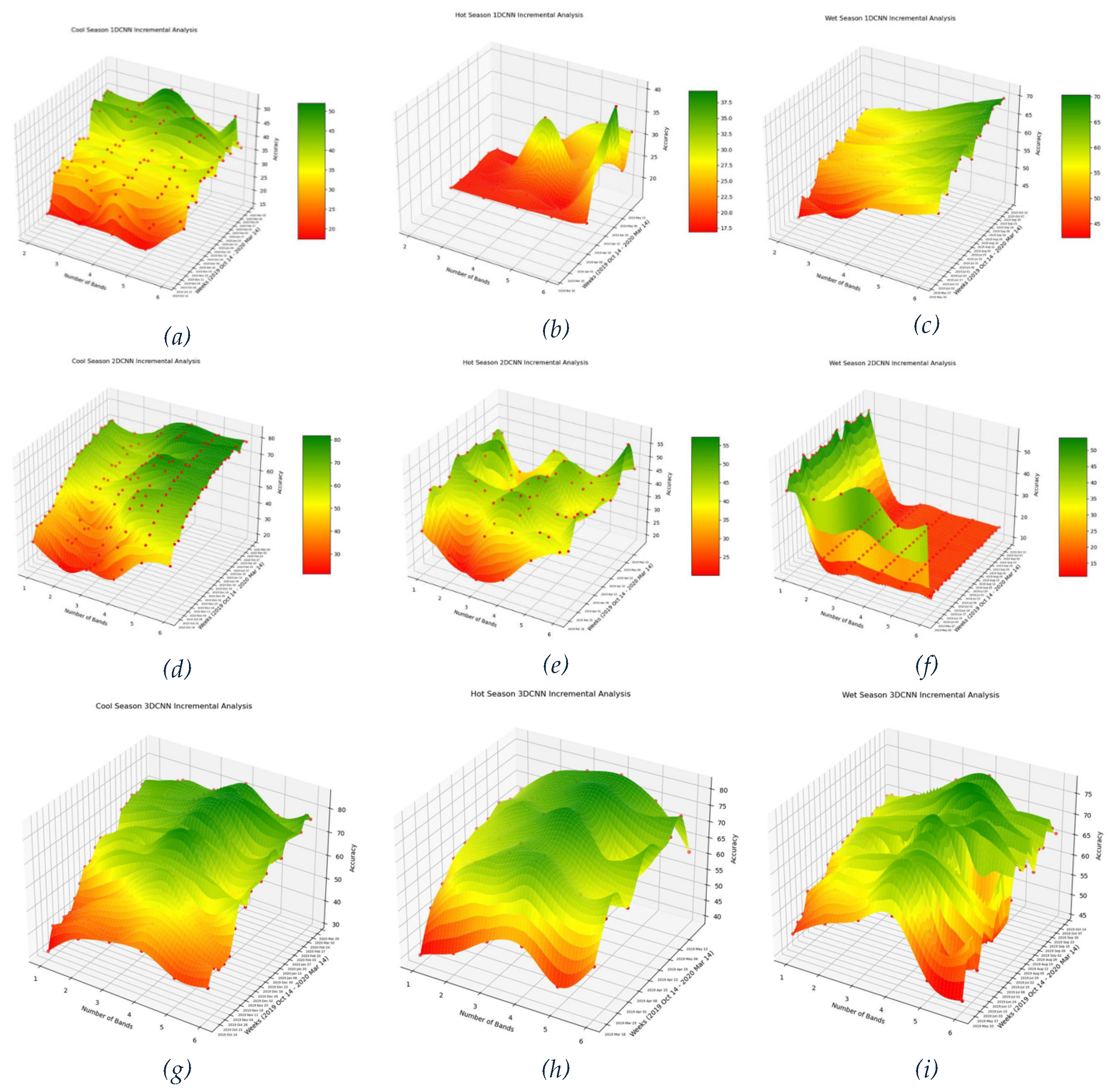
For the 1D CNN-LSTM model, accuracy generally improved as more timesteps and feature bands were added. However, the improvement was gradual and less stable than for the spatial CNN models. This indicates that temporal-spectral profiles alone can support classification but require sufficient seasonal information to become discriminative. In the hot season, where only 10 timesteps were available, the 1D model remained comparatively weak, suggesting that short temporal sequences were not enough to separate several crop classes.
The 2D CNN showed stronger performance under reduced-input settings because it could exploit local spatial patterns in addition to stacked spectral-temporal channels. In the cool season, the 2D CNN reached approximately 70% accuracy around timestep 10, suggesting that spatial context helped compensate for incomplete temporal information. In the hot season, performance varied more strongly, with the study noting a peak of 57.87% using six bands at timestep 9 during the incremental experiment. This indicates that the hot-season performance was sensitive to the specific combination of bands and timesteps.
The 3D CNN showed the clearest advantage in the incremental analysis because it preserved spectral, spatial, and temporal dimensions jointly. In the cool season, the 3D CNN reached an estimated accuracy of approximately 81% around timestep 9, outperforming the corresponding 1D and 2D configurations. In the wet season, the 3D CNN improved with additional timesteps and higher feature-band availability, showing that the model benefited from temporal development patterns when those patterns were sufficiently captured.
Overall, the incremental analysis supports the conclusion that the value of additional input data depends on both season and architecture. More timesteps and bands can improve accuracy, but gains are not always linear. In some cases, additional radar or spectral inputs may introduce noise or limited marginal improvement. The strongest practical implication is that 3D CNNs may support reduced-input seasonal classification when the retained observations capture key crop-growth stages, while 2D CNNs provide a strong operational baseline when spatial structure is more reliable than temporal progression.
3.5. Visual Comparison of Seasonal Classification Maps
The results show that classification performance varied substantially by season and architecture. In general, the two-dimensional and three-dimensional CNN configurations performed better than the one-dimensional baseline because they retained more spatial context. The one-dimensional configuration captured useful temporal and spectral signals, but it was less effective for classes requiring spatial texture, field-structure information, or joint spatio-temporal interpretation. The 2D CNN performed strongly in several seasonal settings, particularly where spatial patterns and stacked multi-temporal channels were sufficient to separate classes. The 3D CNN and the modified 3D CNN were most relevant because they directly tested the value of preserving temporal structure in the model architecture.
Figure 13.
Comparison of zoomed-in areas of predictions across different CNN architecture.
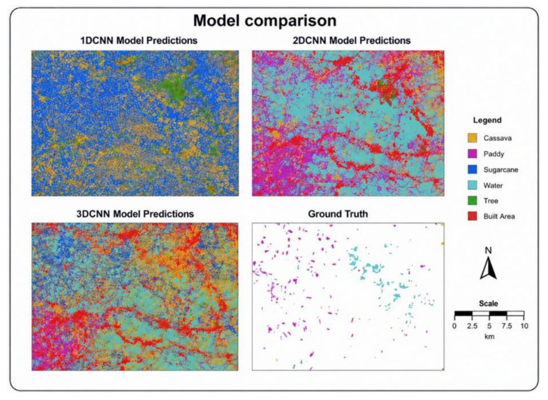
Across the study experiments, the cool season generally produced the strongest classification results, while the hot season was more difficult. The wet season produced intermediate to strong results depending on architecture and class. These seasonal differences are consistent with the agricultural calendar and the quality of observable crop phenology in each period. The hot season appeared more challenging because some classes had weaker separability, fewer reliable temporal cues, or greater confusion with other crop and land-cover types. The wet and cool seasons benefited from clearer vegetation development patterns and, in some cases, stronger class-specific temporal signatures.
Figure 14.
Comparison of seasonal predictions against label data using 3DCNN+DoY model.
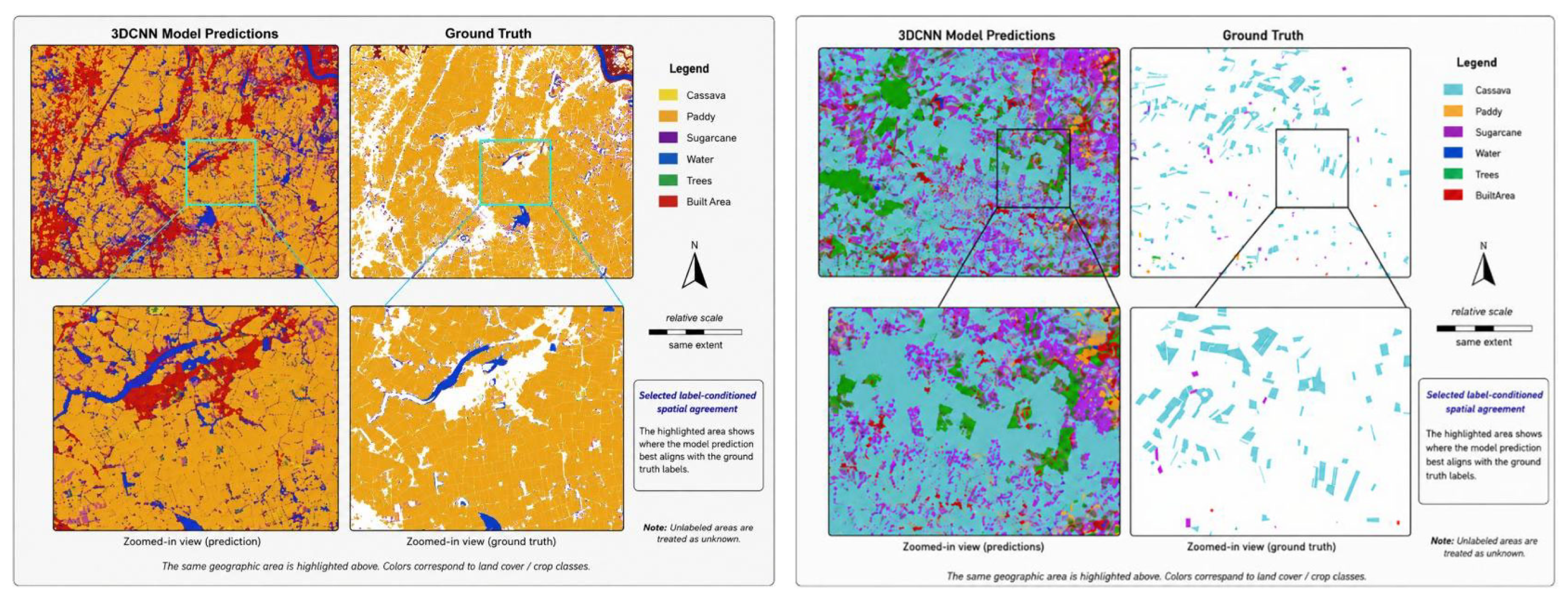
Figure 15.
Comparison of seasonal predictions against label data using 3DCNN+DoY model.
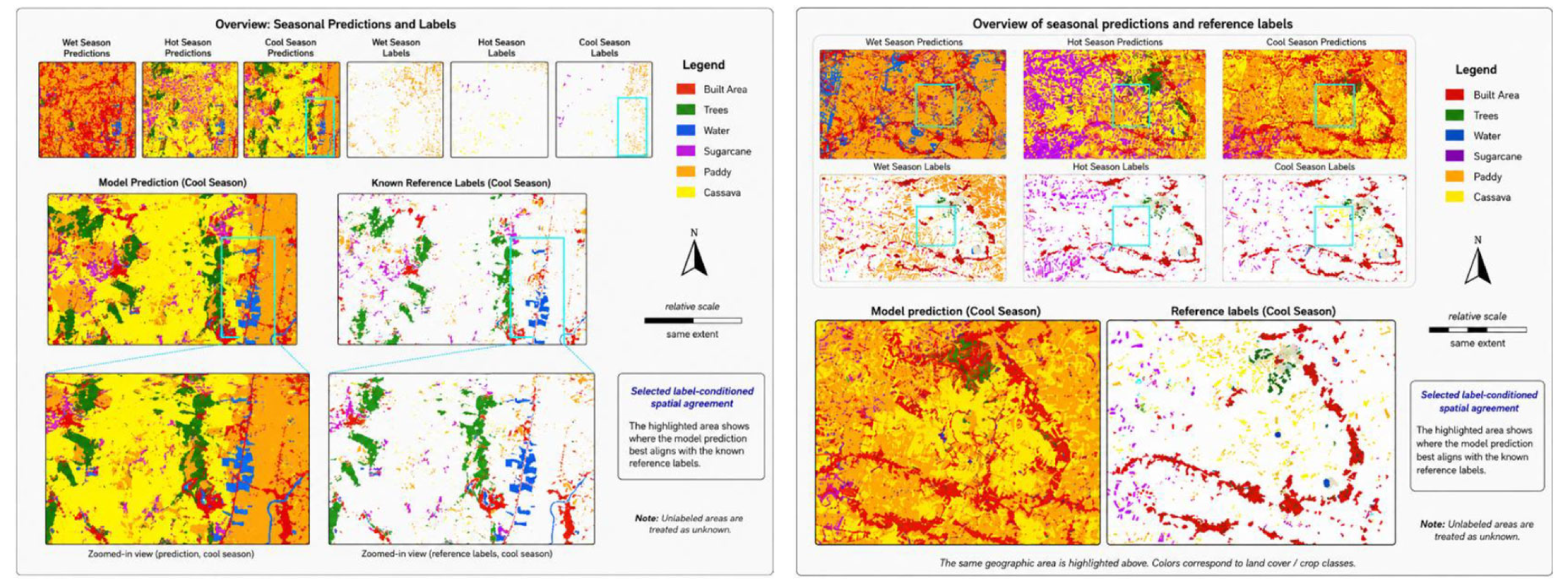
The modified 3D CNN with day-of-year phenological features provided an important research direction for publication. Its strongest result was in the cool season, where it achieved approximately 85% overall accuracy and a weighted F1-score of about 0.85. This suggests that combining spatio-temporal CNN features with explicit growth-stage timing can improve seasonal crop classification when phenological structure is reliable. However, the modified architecture did not uniformly improve every season, indicating that phenological features are useful but not automatically sufficient; their value depends on data quality, crop calendar consistency, and the separability of the target classes in each season.
3.3. Feature Extractor and Transferability
The study also examined the use of CNN-derived features with a Random Forest classifier. This analysis is important because it separates feature learning from the final classification mechanism. The results suggest that CNNs, particularly 3D CNNs, can serve as useful spatial-temporal feature extractors even when a classical classifier performs strongly on the final classification task.
Figure 16.
Transfer learning of pretest-trained CNN layers.
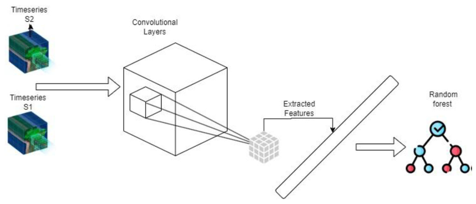
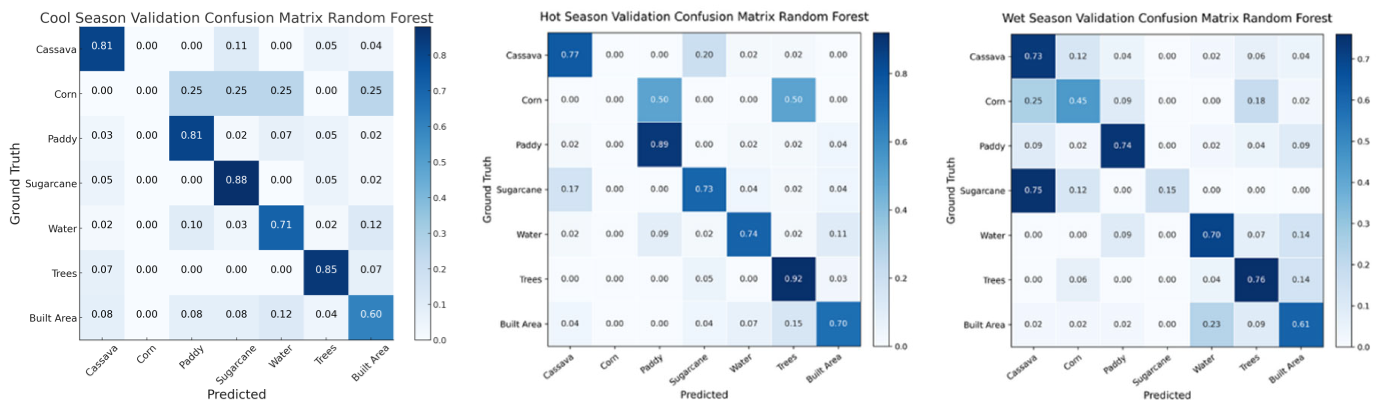
Random Forest achieved strong seasonal performance, with 85% accuracy in the cool season, 80% in the hot season, and 79% in the wet season. These results show that classical classifiers remain competitive when supplied with well-prepared seasonal features. Therefore, the most defensible finding is not that CNNs universally outperform Random Forest, but that CNN representations and classical classifiers may provide complementary strengths.
Figure 17.
Confusion matrix of pretrained CNN layers with Random Forest.
4. Discussion
The results demonstrate that CNN dimensionality substantially influences seasonal crop-classification performance in the Tha Chin River Basin. The 1D CNN-LSTM model provided a useful temporal-spectral baseline, but its lower overall accuracy across seasons indicates that temporal profiles alone were not sufficient to distinguish all crop and land-cover classes. This limitation was most visible in classes requiring spatial context or field-level structure, such as cassava, sugarcane, maize, and built-up areas. In contrast, the 2D CNN achieved more consistent performance across seasons by incorporating local spatial information from image patches. This suggests that field texture, neighborhood structure, and spatial continuity are important for crop discrimination in heterogeneous agricultural landscapes.
The comparison between 2D and 3D CNN architectures shows that preserving temporal structure can be beneficial, but only when the seasonal signal is reliable. The 3D CNN was designed to learn spatial and temporal features jointly, which makes it conceptually well suited for multi-temporal crop classification. However, its performance varied strongly by season, with weaker results in the hot season. This indicates that higher-dimensional CNNs do not automatically improve performance when temporal coverage is short, crop separability is weak, or validation samples contain noisy or imbalanced class distributions. The result is important because it prevents an overgeneralized interpretation that 3D CNNs are always superior for seasonal remote-sensing classification.
The modified 3D CNN with Day-of-Year (DoY) phenological features produced the strongest CNN-based result in the cool season, reaching approximately 85% overall accuracy and a weighted F1-score of 0.85. This suggests that explicit phenological timing information can improve classification when crop-growth stages are clearly represented in the time series. The DoY features helped the model incorporate green-up, peak growth, and senescence timing, which can be useful for separating crops with similar spectral signatures but different growth calendars. However, the weaker hot- and wet-season performance shows that phenological descriptors are sensitive to planting-date uncertainty, cloud-related gaps, weekly aggregation, and label reliability. Therefore, DoY integration should be interpreted as a promising direction rather than a fully solved solution.
Figure 18.
Comparative Overview of Model Performance across Seasons.
Class-wise results further show that model performance was not uniform across crop and land-cover categories. Water and trees were generally more stable because they have more distinct spectral, radar, and spatial characteristics. Paddy rice also performed well in several experiments, especially where water-related and vegetation-growth signals were visible. By contrast, maize remained unstable, often showing weak precision or inconsistent recall. Cassava and sugarcane were frequently confused, especially in seasons where their canopy structure or vegetation-index trajectories overlapped. Built-up areas also showed variable performance, likely because mixed pixels and fragmented settlement-agriculture boundaries complicated classification. These patterns show that class-wise precision, recall, and F1-score are necessary for interpreting model behavior; overall accuracy alone would hide important weaknesses in minority or ambiguous classes.
Figure 19.
Comparative Overview of model comparisons at respective landcover types.
The learning curves support these findings by showing that model convergence depended on both architecture and season. The 2D CNN generally showed steady learning and stable validation accuracy, although validation-loss fluctuations indicated some sensitivity to seasonal noise and class composition. The 3D CNN showed more variable convergence, particularly in the hot season, where unstable validation behavior aligned with weaker overall accuracy. The modified 3D CNN showed the clearest convergence in the cool season, supporting the value of phenological timing under favorable seasonal conditions. These learning patterns indicate that architecture evaluation should consider not only final accuracy, but also training stability and generalization behavior.
The incremental analysis provides an operational interpretation of the results. Accuracy generally improved as more timesteps and feature bands were added, but the gain was not linear and depended on season and architecture. The 1D CNN relied strongly on sufficient temporal-spectral information, while the 2D CNN could partially compensate through spatial features. The 3D CNN showed the strongest potential for reduced-input seasonal mapping when key phenological stages were captured. This finding is important for early-season crop monitoring because operational decisions often need to be made before a full seasonal time series is available.
The strong Random Forest results also shape the interpretation of the CNN experiments. Random Forest achieved competitive performance across seasons, including approximately 85%, 80%, and 79% overall accuracy in the cool, hot, and wet seasons, respectively. This indicates that classical machine-learning approaches remain robust when feature engineering is strong. The contribution of the CNN models should therefore be framed around representation learning and architecture behavior rather than a simple claim that deep learning outperforms traditional methods. A more defensible interpretation is that CNNs, especially 3D CNNs, can provide useful spatio-temporal feature representations, while Random Forest remains a strong baseline or downstream classifier.
These findings are consistent with recent remote-sensing crop-classification studies showing that spatial context and temporal phenology are both important for crop mapping. The ingested Remote Sensing 2025 study reported that 2D CNN-GRU outperformed 1D CNN-RNN models because 2D spatial feature extraction improved crop-map coherence while recurrent layers modeled temporal dependencies. The present study reaches a complementary conclusion under a different architecture design: 2D CNNs improve performance by adding spatial context, while 3D CNNs offer a direct convolutional approach to learning spatial-temporal datacubes. However, the Thailand case also shows lower and more variable accuracies than the northern Italy study, likely due to differences in label quality, crop classes, seasonal cloud conditions, radar-optical fusion, planting-date uncertainty, and landscape heterogeneity.
Several limitations should be noted. First, label quality is a major constraint because seasonal crop labels depend partly on recorded planting dates, which may not always match actual field phenology. Second, weekly aggregation and temporal interpolation simplify data preparation but may remove short-term phenological detail. Third, wet-season cloud cover and moisture variability can alter optical and radar signals even after preprocessing. Fourth, class imbalance affects model training and evaluation, especially for maize and other underrepresented categories. Finally, the study compares CNN dimensionality but does not directly test CNN-RNN or transformer-based architectures under the same Thailand dataset. Future work should therefore validate the CNN results using repeated random-seed experiments, test hybrid 2D CNN-GRU and transformer baselines, improve field-label reliability, and incorporate ancillary crop-calendar, weather, soil, and irrigation information.
Figure 20.
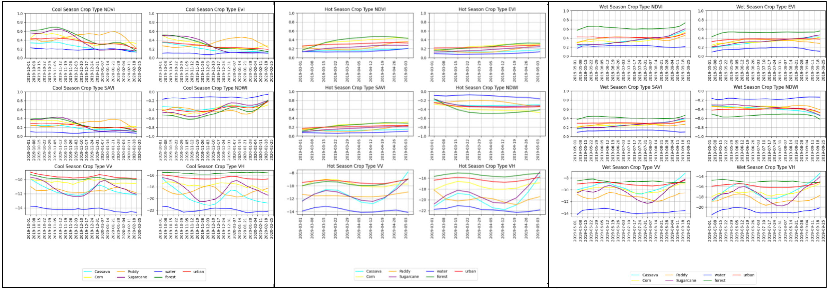
Seasonal Timeseries Profile of Land cover and Crops.
5. Conclusions
This study evaluated 1D CNN-LSTM, 2D CNN, 3D CNN, and modified 3D CNN + DoY architectures for seasonal crop and land-cover classification in Thailand’s Tha Chin River Basin using multi-temporal Sentinel-1 and Sentinel-2 data. The results show that CNN dimensionality affects classification performance because each architecture represents spectral, spatial, and temporal information differently.
The 1D CNN-LSTM model captured temporal-spectral patterns but was limited by the absence of explicit spatial context. The 2D CNN provided the most consistent pure-CNN performance across seasons, demonstrating the value of local spatial structure for crop and land-cover discrimination. The 3D CNN offered a stronger spatial-temporal representation, particularly for reduced-input seasonal analysis, but its performance was sensitive to seasonal data quality and crop separability. The modified 3D CNN + DoY model achieved the strongest CNN-based result in the cool season, suggesting that phenological timing features can improve classification when crop-growth stages are reliable and well aligned with the satellite time series.
Class-wise evaluation showed that water, trees, and paddy rice were generally classified more reliably than maize, cassava, sugarcane, and built-up areas. The main sources of error were crop-class confusion, mixed pixels, class imbalance, and planting-date uncertainty. These findings confirm that overall accuracy must be interpreted together with precision, recall, F1-score, confusion matrices, and learning-curve behavior.
The study also shows that Random Forest remains a strong baseline when applied to well-engineered seasonal features. Therefore, the main contribution is not a claim that CNNs universally outperform classical machine-learning models, but rather an analysis of how CNN input dimensionality changes seasonal crop-classification behavior. The findings support the use of spatial and spatial-temporal CNN architectures for crop mapping while establishing a baseline for future hybrid CNN-RNN, transformer-based, and feature-extractor approaches in climate-affected agricultural regions.
Author Contributions
Conceptualization, Z.T.H. and S.N.; methodology, Z.T.H., S.N., C.M, S.C; software, Z.T.H.; validation, Z.T.H., S.N. and C.N.; formal analysis, Z.T.H.; investigation, Z.T.H., S.N., C.M.; resources, Z.T.H, S.N.; data curation, Z.T.H.; writing—original draft preparation, Z.T.H.; writing—review and editing, Z.T.H., C.M.; visualization, Z.T.H.; supervision, S.N., C.M.; project administration, S.N., T.K; funding acquisition, S.N. All authors have read and agreed to the published version of the manuscript.
Funding
This research was funded and conducted as part of the first author’s master thesis and was supported by Loom Nam Khong Pijai scholarship provided by the Royal Thai Government through the Asian Institute of Technology.
Data Availability Statement
Data will be made available on request.
Acknowledgments
The authors used ChatGPT ( Open AI, ChatGPT-4, 2024 version ) for grammar correction and improve English writings. After using such tool, the authors reviewed, revised and verified all the content and take full responsibility of the content of the publication. The authors gratefully acknowledge the Department of Agricultural Extension (DOAE), Thailand, for providing the crop-label dataset used in this study and for facilitating and supporting the associated field surveys. The authors also gratefully acknowledge the Hydro-Informatics Institute (HII), Thailand, for providing the supporting dataset used in this research.
Conflicts of Interest
S.N. is a Guest Editor of the Special Issue in which this manuscript is submitted and has been recused from its editorial handling. The authors declare no other conflicts of interest.
Abbreviations
The following abbreviations are used in this manuscript:
| MDPI | Multidisciplinary Digital Publishing Institute |
| DOAJ | Directory of open access journals |
| TLA | Three letter acronym |
| LD | Linear dichroism |
| CNN | Convolutional Neural Networks |
| DoY | Day of year |
| NDVI | Normalized Difference Vegetation Index |
| EVI | Enhanced Vegetation Index |
| NDWI | Normalized difference Water Index |
| SAVI | Soil Adjusted Vegetation Index |
References
- Sinha, P.; Kumar, L.; Reid, N. SEASONAL LAND USE / LAND COVER MAPPING: ACCURACY COMPARISON OF VARIOUS BAND COMBINATIONS. [PubMed]
- Kerner, H.; Sahajpal, R.; Skakun, S.; Becker-Reshef, I.; Barker, B.; Hosseini, M.; Puricelli, E.; Gray, P. Resilient In-Season Crop Type Classification in Multispectral Satellite Observations using Growth Stage Normalization. 2020. [Google Scholar] [CrossRef]
- Kiptala, J. K.; Mohamed, Y.; Mul, M. L.; Cheema, M. J. M.; Van Der Zaag, P. Land use and land cover classification using phenological variability from MODIS vegetation in the Upper Pangani River Basin, Eastern Africa. Phys. Chem. Earth 2013, 66, 112–122. [Google Scholar] [CrossRef]
- Zhong, L.; Hawkins, T.; Biging, G.; Gong, P. A phenology-based approach to map crop types in the San Joaquin Valley, California. Int. J. Remote Sens. 2011, 32, 7777–7804. [Google Scholar] [CrossRef]
- Mao, M.; Zhao, H.; Tang, G.; Ren, J. In-Season Crop Type Detection by Combing Sentinel-1A and Sentinel-2 Imagery Based on the CNN Model. Agronomy 2023, 13. [Google Scholar] [CrossRef]
- Belgiu, M.; Csillik, O. Sentinel-2 cropland mapping using pixel-based and object-based time-weighted dynamic time warping analysis. Remote Sens. Environ. 2018, 204, 509–523. [Google Scholar] [CrossRef]
- Stournaras, S.; Loukatos, D.; Arvanitis, K. G.; Kalatzis, N. Crop Identification by Machine Learning Algorithm and Sentinel-2 Data; MDPI AG, 2022; p. 20. [Google Scholar]
- Wu, J.; Jin, S.; Zhu, G.; Guo, J. Monitoring of Cropland Abandonment Based on Long Time Series Remote Sensing Data: A Case Study of Fujian Province, China. Agronomy 2023, 13. [Google Scholar] [CrossRef]
- Zhou, X.; Wang, J.; Shan, B.; He, Y. Early-Season Crop Classification Based on Local Window Attention Transformer with Time-Series RCM and Sentinel-1. In Remote Sens. (Basel).; 2024; p. 16. [Google Scholar]
- Belgiu, M.; Zhou, Y.; Marshall, M.; Stein, A. Dynamic time warping for crops mapping. In International Archives of the Photogrammetry, Remote Sensing and Spatial Information Sciences—ISPRS Archives; International Society for Photogrammetry and Remote Sensing, 2020; Vol. 43, pp. 947–951. [Google Scholar]
- Peng, D.; Huete, A. R.; Huang, J.; Wang, F.; Sun, H. Detection and estimation of mixed paddy rice cropping patterns with MODIS data. Int. J. Appl. Earth Obs. Geoinf. 2011, 13, 13–23. [Google Scholar] [CrossRef]
- Hao, P.; Di, L.; Zhang, C.; Guo, L. Transfer Learning for Crop classification with Cropland Data Layer data (CDL) as training samples. Sci. Total Environ. 2020, 733. [Google Scholar] [CrossRef] [PubMed]
- Wang, Q.; Yang, B.; Li, L.; Liang, H.; Zhu, X.; Cao, R. Within-Season Crop Identification by the Fusion of Spectral Time-Series Data and Historical Crop Planting Data. Remote Sens. . 2023, 15. [Google Scholar] [CrossRef]
- Azar, R.; Villa, P.; Stroppiana, D.; Crema, A.; Boschetti, M.; Brivio, P. A. Assessing in-season crop classification performance using satellite data: A test case in Northern Italy. Eur. J. Remote Sens. 2016, 49, 361–380. [Google Scholar] [CrossRef]
- Gallo, I.; Ranghetti, L.; Landro, N.; La Grassa, R.; Boschetti, M. In-season and dynamic crop mapping using 3D convolution neural networks and sentinel-2 time series. ISPRS J. Photogramm. Remote Sens. 2023, 195, 335–352. [Google Scholar] [CrossRef]
Disclaimer/Publisher’s Note: The statements, opinions and data contained in all publications are solely those of the individual author(s) and contributor(s) and not of MDPI and/or the editor(s). MDPI and/or the editor(s) disclaim responsibility for any injury to people or property resulting from any ideas, methods, instructions or products referred to in the content. |
© 2026 by the authors. Licensee MDPI, Basel, Switzerland. This article is an open access article distributed under the terms and conditions of the Creative Commons Attribution (CC BY) license (http://creativecommons.org/licenses/by/4.0/).
Copyright: This open access article is published under a Creative Commons CC BY 4.0 license, which permit the free download, distribution, and reuse, provided that the author and preprint are cited in any reuse.