Spiking Neural Networks from Signals to Silicon:An End-to-End Survey of Dynamics, Learning,Architectures, Toolchains, Neuromorphic Hardware,and Deployment

1. Scope, Review Method, and the Event Contract

An SNN is not deployable merely because its activations are called spikes. A deployed system must preserve the meaning of an event while crossing a sensor interface, a numerical simulator, a trained graph, a compiler, a routing fabric, and an output decoder. We call the shared specification across those layers the event contract. Its fields are event semantics, time base, retained state, numerical precision, locality, adaptation, and measurement boundary. This choice separates SNNs from the broader neuromorphic category. Analog in-memory accelerators, continuous-time dynamical systems, and sparse ANNs can be neuromorphic without exchanging discrete spikes; conversely, an SNN simulated as dense tensors can be spiking at the model level without event-driven execution.

Figure 1. The survey’s organizing unit is a cross-layer event contract. A change at any boundary can densify activity, alter temporal meaning, introduce unsupported state, or move cost outside the measured accelerator.

Figure 1. The survey’s organizing unit is a cross-layer event contract. A change at any boundary can densify activity, alter temporal meaning, introduce unsupported state, or move cost outside the measured accelerator.

The evidence collection began with foundational neuron and plasticity papers, expanded through learning and conversion families, and then followed executable paths through software, intermediate representations, chips, sensors, benchmarks, and applications. Publisher records, institutional pages, primary papers, and official project documentation were checked before a source entered the bibliography. Surveys and roadmaps identify coverage gaps and terminology, not numerical ground truth. Vendor specifications are treated as platform descriptions. They are not ranked beside independently measured systems unless workload and boundary match. This distinction matters because neuromorphic systems differ in whether reported power includes memory, host, sensor, I/O, and idle energy [1,2].

Our synthesis asks four questions at every layer. What information does an event carry? Which state must persist between events? Which resources scale with network size, event count, and duration? Which measurement demonstrates the claimed advantage? This produces an end-to-end account rather than a chronology of named models.

Table 1. The event contract and typical contract violations.

Field	Required declaration	Frequent violation
Semantics	polarity, address, magnitude, payload	graded values counted as binary spikes
Time	continuous, ticked, binned, windowed	latency compared at different windows
State	membrane, trace, delay, adaptation	hidden host-side state omitted
Precision	weights, state, threshold, accumulator	floating model mapped to low-bit core
Locality	fan-in/out, multicast, memory scope	synaptic operations ignore routing cost
Adaptation	offline, chip-local, global update	on-chip learning claimed for off-chip loop
Boundary	core, board, host, sensor-to-action	accelerator power called system energy

Table 1. The event contract and typical contract violations.

Field	Required declaration	Frequent violation
Semantics	polarity, address, magnitude, payload	graded values counted as binary spikes
Time	continuous, ticked, binned, windowed	latency compared at different windows
State	membrane, trace, delay, adaptation	hidden host-side state omitted
Precision	weights, state, threshold, accumulator	floating model mapped to low-bit core
Locality	fan-in/out, multicast, memory scope	synaptic operations ignore routing cost
Adaptation	offline, chip-local, global update	on-chip learning claimed for off-chip loop
Boundary	core, board, host, sensor-to-action	accelerator power called system energy

2. Why Spikes Can Help, and Why They Often Do Not

For layer ℓ over duration T, a first-order event workload is

$$N_{\mathrm{synop}}^{(\ell )}={\displaystyle \sum _{t=1}^T}\sum _i{s}_i^{(\ell -1)}\left[t\right]d_i^{(\ell )},$$

(1)

where $d_i$ is the number of delivered outgoing synapses after mapping. Energy is better approximated by

$$E_{\mathrm{sys}}=E_{\mathrm{sense}}+E_{\mathrm{encode}}+E_{\mathrm{route}}+E_{\mathrm{syn}}+E_{\mathrm{state}}+E_{\mathrm{io}}+E_{\mathrm{host}}+E_{\mathrm{idle}}T.$$

(2)

A sparse neuron trace reduces only some terms. Long windows increase state updates and idle cost; multicast replication increases routing; frame conversion can dominate encoding; and an unsupported operator can return execution to a dense host. TrueNorth demonstrated that co-locating state and event communication can produce low-power inference [3], but that result is an architectural example, not a theorem that applies to every SNN.

3. Mathematical Foundations: Spikes, State, and Codes

3.1. Spike Trains and Synaptic Dynamics

A spike train is a point process $s_i\left(t\right)={\sum }_k\delta (t-t_i^k)$. A causal synapse filters events, following the standard point-process treatment of neuronal dynamics [4],

$${\tau }_s{\dot{I}}_i\left(t\right)=-I_i\left(t\right)+\sum _j{w}_{ij}{s}_j(t-d_{ij}),$$

(3)

where $d_{ij}$ exposes a deployment constraint: many accelerators support only integer or bounded delays. The current-based leaky integrate-and-fire (LIF) neuron is

$${\tau }_m{\dot{u}}_i=-(u_i-u_{\mathrm{rest}})+R{I}_i\left(t\right),s_i\left(t\right)=\Theta (u_i-\vartheta ),$$

(4)

followed by subtractive or hard reset and an optional refractory interval. With zero-order hold and step $\Delta t$,

$$\begin{array}{cc}\hfill u_i[t+1]& =\beta u_i\left[t\right]+\sum _j{w}_{ij}{s}_j\left[t\right]-\vartheta s_i\left[t\right],\hfill \end{array}$$

(5)

$$\begin{array}{cc}\hfill s_i\left[t\right]& =H(u_i\left[t\right]-\vartheta ),\beta =e^{-\Delta t/{\tau }_m}.\hfill \end{array}$$

(6)

Thus changing $\Delta t$ without transforming $\beta$, delays, and input scale changes the model. NIR addresses this portability problem by defining continuous-time primitives and explicit transformations [5].

Figure 2. A spiking neuron is a state machine. Hardware must implement the update, threshold, reset, and any adaptation with compatible time and precision.

Figure 2. A spiking neuron is a state machine. Hardware must implement the update, threshold, reset, and any adaptation with compatible time and precision.

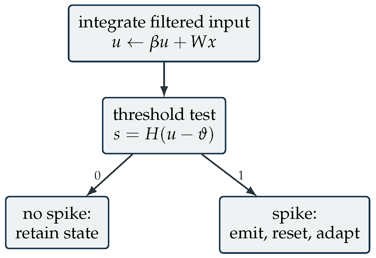
Biophysical Hodgkin–Huxley dynamics model voltage-dependent ionic conductances and serve as a reference for neural excitability [6]. LIF removes channel state for efficiency. Izhikevich adds a recovery variable and reset to reproduce diverse firing patterns, while AdEx adds an exponential threshold current and adaptation [7,8]. The appropriate model is therefore determined by task-relevant dynamics and target primitives, not biological detail alone.

3.2. Coding and Decoding

Rate coding estimates $r_i=N_i/T$ and trades decision latency for variance. Time-to-first-spike (TTFS) maps magnitude to latency, often as $t_i=t_0-\kappa log(x_i+ϵ)$, and can stop after one event per neuron. Phase, rank-order, burst, population, and delta-modulation codes make different assumptions about clocks and downstream decoders. No code is intrinsically sparse: Poisson rate encoding of static pixels can create more traffic than a compact fixed-point tensor.

For output, spike count, first-spike class, maximum membrane, filtered readout, and population vector are not interchangeable. A decision rule $\widehat{y}=arg{max}_c{\sum }_t{s}_c\left[t\right]$ cannot claim TTFS latency. Early exit requires a confidence process and must report the stopping distribution, not only a maximum window.

3.3. Plasticity

Pair-based STDP is often written

$$\Delta w_{ij}=\left\{\begin{array}{cc}{A}_{+}{e}^{-\Delta t/{\tau }_{+}},\hfill & \Delta t=t_{\mathrm{post}}-t_{\mathrm{pre}}>0,\hfill \\ -A_{-}{e}^{\Delta t/{\tau }_{-}},\hfill & \Delta t<0.\hfill \end{array}\right.$$

(7)

Bi and Poo established timing-dependent potentiation and depression under specific experimental conditions [9]. Supervised temporal rules such as the Tempotron use spike timing for task-level decisions [10]. Practical learning rules also depend on weight, rate, voltage, neuromodulation, and homeostasis. Treating the pair rule as a complete task-level optimizer confuses a local synaptic observation with global credit assignment.

Table 2. Neuron models as mathematical and deployment contracts.

Model	State equation or mechanism	Dynamic state	Strength	Deployment cost	Typical mismatch
IF	$u[t+1]=u\left[t\right]+I\left[t\right]-\vartheta s\left[t\right]$	voltage	cheapest temporal accumulator	add, compare, reset	no leak; window-dependent rate
LIF	Eq. (5)	voltage	useful accuracy/cost balance	decay multiply or shift	time constant discretization
ALIF	LIF plus adaptive threshold trace	voltage, adaptation	longer temporal memory	extra state and decay	unsupported adaptive threshold
AdEx	exponential current plus adaptation	voltage, adaptation	rich excitability	nonlinear function or approximation	analog/digital parameter mismatch
Izhikevich	quadratic voltage and recovery	two variables	many firing regimes	multiplies, branch/reset	limited native core support
Conductance	reversal-potential synaptic current	voltage, conductances	closer synaptic physics	several states per neuron	expensive tensor training
Multi-compartment	coupled dendritic compartments	vector state	spatial and nonlinear dendrites	routing plus compartment state	graph expansion during lowering
Stochastic	probabilistic threshold/escape	state plus RNG	sampling and uncertainty	random source and distribution	simulator/hardware RNG mismatch

Table 2. Neuron models as mathematical and deployment contracts.

Model	State equation or mechanism	Dynamic state	Strength	Deployment cost	Typical mismatch
IF	$u[t+1]=u\left[t\right]+I\left[t\right]-\vartheta s\left[t\right]$	voltage	cheapest temporal accumulator	add, compare, reset	no leak; window-dependent rate
LIF	Eq. (5)	voltage	useful accuracy/cost balance	decay multiply or shift	time constant discretization
ALIF	LIF plus adaptive threshold trace	voltage, adaptation	longer temporal memory	extra state and decay	unsupported adaptive threshold
AdEx	exponential current plus adaptation	voltage, adaptation	rich excitability	nonlinear function or approximation	analog/digital parameter mismatch
Izhikevich	quadratic voltage and recovery	two variables	many firing regimes	multiplies, branch/reset	limited native core support
Conductance	reversal-potential synaptic current	voltage, conductances	closer synaptic physics	several states per neuron	expensive tensor training
Multi-compartment	coupled dendritic compartments	vector state	spatial and nonlinear dendrites	routing plus compartment state	graph expansion during lowering
Stochastic	probabilistic threshold/escape	state plus RNG	sampling and uncertainty	random source and distribution	simulator/hardware RNG mismatch

4. Learning and Conversion

The derivative of $H(u-\vartheta )$ vanishes almost everywhere and is undefined at threshold. Surrogate-gradient training keeps the hard spike in the forward pass and substitutes a smooth derivative in the backward pass,

$${\displaystyle \frac{\partial s}{\partial u}}\approx {\sigma }_{\alpha }^{\prime }(u-\vartheta ),{\sigma }_{\alpha }^{\prime }\left(z\right)\in \left\{{\displaystyle \frac{\alpha }{{(1+\alpha |z\left|\right)}^2}},\alpha max(0,1-|\alpha z\left|\right)\right\}.$$

(8)

This produces a biased estimator but makes deep SNN optimization practical [11,12,13]. Unrolling Eq. (5) gives

$${\displaystyle \frac{\partial \mathcal{L}}{\partial w_{ij}}}=\sum _t{\displaystyle \frac{\partial \mathcal{L}}{\partial s_i\left[t\right]}}{\sigma }_{\alpha }^{\prime }(u_i\left[t\right]-\vartheta ){\displaystyle \frac{\partial u_i\left[t\right]}{\partial w_{ij}}},$$

(9)

and requires neuron state, surrogate choice, reset gradient, loss timing, and truncation policy. Memory grows roughly as $O\left(T{\sum }_l{N}_l\right)$ before checkpointing. Long horizons therefore threaten training memory even when inference events are sparse.

Figure 3. Three learning paths expose different deployment contracts. Conversion inherits ANN operators and latency error; direct gradient training consumes temporal-state memory; local and online rules restrict the credit signal but can adapt without storing the full trajectory.

Figure 3. Three learning paths expose different deployment contracts. Conversion inherits ANN operators and latency error; direct gradient training consumes temporal-state memory; local and online rules restrict the credit signal but can adapt without storing the full trajectory.

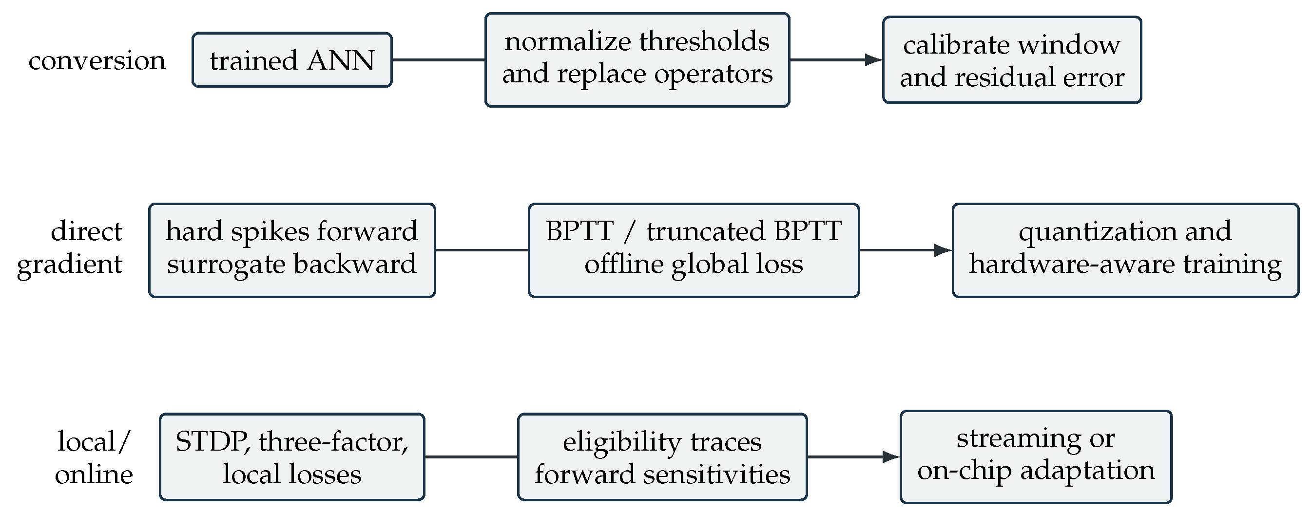
ANN-to-SNN conversion interprets a rectified activation as a firing rate [14,15,16]. For an IF neuron driven by constant z, the finite-window approximation obeys an error of the form

$$\left|z-\vartheta {\displaystyle \frac{N\left(T\right)}{T}}\right|\le {\displaystyle \frac{\vartheta +\left|u\right(T)-u(0\left)\right|}{T}},$$

(10)

before clipping, quantization, max-pooling, normalization folding, and residual-path errors. Larger T reduces rate error but increases latency and state activity. Threshold balancing and residual membrane treatments improve this trade-off, yet converted graphs remain constrained by target operator support.

Exact event-based gradients differentiate continuous trajectories and apply jump conditions at spike times [17]. They remove the surrogate at the cost of assumptions about event ordering, differentiability between events, and spike creation or deletion. Eligibility and forward-mode methods retain causal traces or sensitivities for online updates [18,19]. Eligibility methods factor a gradient into a local trace and a learning signal, $\Delta w_{ij}\propto {\sum }_t{L}_i\left[t\right]e_{ij}\left[t\right]$. Their central benefit is causal, streaming state; their limitation is approximate global credit or an additional learning channel.

Hardware-aware training inserts weight/state quantization, fan-in limits, delay grids, noisy parameters, and measured transfer functions into the forward model. Mixed-signal studies show that training against the realized substrate can recover performance lost to mismatch, but the resulting parameters may be device-specific. That is a fleet-management issue, not merely a training trick.

5. Network Architectures and Temporal Computation

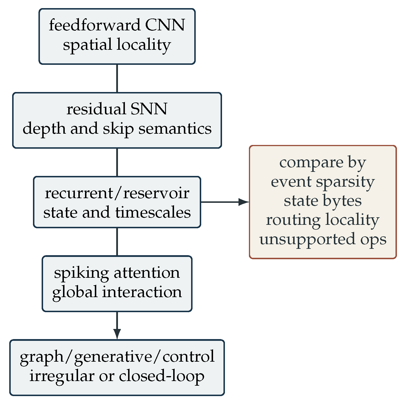
The architectural question is not whether a convolution, recurrence, or attention block can contain spiking neurons. It is whether its complete data path preserves event-driven operations. Batch normalization folded into weights is cheap at inference, while LayerNorm, softmax, dense residual additions, and attention score products can reintroduce floating-point work. This distinction separates spike-valued interfaces from spike-driven execution.

Convolutional SNNs share weights spatially and map well when event addresses index kernels. Their cost depends on active input events and delivered kernel fan-out, not the dense multiply-accumulate count alone. Residual SNNs improve depth optimization but require careful placement of the spike function: an analog-valued skip path can dominate arithmetic and violate a binary event interface. Recurrent SNNs expose their strongest inductive bias on streaming tasks, because membrane, synaptic, and adaptation state provide multiple timescales. Reservoirs train only a readout but spend neurons and routing on a fixed recurrent projection [20].

Spiking attention replaces some dense attention operations with spike-form queries, keys, and values [21,22]. A generic causal block can be written

$$\begin{array}{cc}\hfill S_Q\left[t\right]& =H(W_{Q}S\left[t\right]-{\vartheta }_Q),S_K\left[t\right]=H(W_{K}S\left[t\right]-{\vartheta }_K),\hfill \end{array}$$

(11)

$$\begin{array}{cc}\hfill A\left[t\right]& =\mathcal{N}\left(S_Q\left[t\right]S_K{\left[t\right]}^{\top }\right),Y\left[t\right]=H(A\left[t\right]S_V\left[t\right]-{\vartheta }_Y),\hfill \end{array}$$

(12)

where $\mathcal{N}$ may be scaling, normalization, or a learned spiking operator. Binary operands do not guarantee cheap attention: the all-pairs token interaction remains dense unless the implementation exploits token or channel sparsity. Reported operation-based energy estimates must therefore be separated from measured neuromorphic execution.

Figure 4. Architecture families should be compared by executable event, state, and communication paths, not by neuron labels alone.

Figure 4. Architecture families should be compared by executable event, state, and communication paths, not by neuron labels alone.

Architecture search adds neuron type, time steps, firing rate, precision, and target mapping to conventional depth/width choices. A useful objective is multi-criteria,

$$\underset{a,w}{min}{\mathcal{L}}_{\mathrm{task}}+{\lambda }_E\widehat{E}(a,w)+{\lambda }_L\widehat{L}(a,w)+{\lambda }_M\widehat{M}(a,w),$$

(13)

subject to fan-in, fan-out, supported-state, and routing constraints. Proxy terms must be calibrated on the target; otherwise search optimizes an imagined accelerator.

6. Data, Tasks, and Benchmark Validity

Static frames, converted event streams, native event sensors, and synthetic spike trains test different propositions. Converting MNIST or CIFAR through camera motion supplies timestamps but preserves the source dataset’s static object bias [23,24]. Native DVS gestures test motion and illumination-change sensing, while SHD/SSC represent auditory waveforms as cochlear events [25]. A benchmark suite should therefore cross two axes: provenance (native, converted, simulated) and task output (classification, detection, regression, generation, control).

Accuracy must be paired with window length, time step, firing statistics, state precision, and preprocessing. NeuroBench separates algorithm and system tracks so functional metrics can coexist with latency, throughput, power, and energy [1]. For early-exit systems report $P(T_{\mathrm{decision}}\le t)$ and tail latency, not only mean accuracy.

7. Software and Simulation

Equation-oriented simulators prioritize arbitrary dynamics [26]; neuroscience engines prioritize large networks and distributed simulation; deep-learning libraries prioritize automatic differentiation and GPUs [27]; vendor stacks prioritize executable subsets. Portable APIs and hybrid modeling systems address different parts of this fragmentation [28,29]. These goals create semantic gaps. A framework can train ALIF with floating state but a target may offer LIF with integer decay. Export succeeds syntactically only if the transformation preserves dynamics.

Table 3. Coding schemes and their system consequences.

Code	Information carrier	Event budget	Main advantage	Main loss	Hardware demand	Suitable input
Rate	count in T	medium–high	noise averaging	latency and energy scale with T	counters/windows	stationary intensity
Poisson rate	stochastic count	high	convenient training augmentation	sampling variance	RNG or offline encoder	static frames
TTFS	first event time	at most one/unit	low event count, early exit	timing sensitivity	fine timestamps/delays	normalized features
Rank order	event ordering	one/few	invariant to global time scale	loses amplitude gaps	ordered queue	saliency sequences
Phase	phase relative to oscillation	sparse	multiplexed temporal reference	global clock/phase needed	phase state	rhythmic signals
Burst	intra-burst count/timing	adaptive	high dynamic range	local event explosion	burst-capable neuron	transient strength
Population	distributed receptive fields	configurable	robustness and precision	more neurons/events	parallel fan-out	low-dimensional sensors
Delta/sigma-delta	change since last event	signal-dependent	native streaming sparsity	drift and threshold tuning	stateful encoder	audio, motion, control
Direct current	analog value each step	no input spikes	accurate and simple training	input layer not event-driven	multiply each tick	frame benchmarks

Table 3. Coding schemes and their system consequences.

Code	Information carrier	Event budget	Main advantage	Main loss	Hardware demand	Suitable input
Rate	count in T	medium–high	noise averaging	latency and energy scale with T	counters/windows	stationary intensity
Poisson rate	stochastic count	high	convenient training augmentation	sampling variance	RNG or offline encoder	static frames
TTFS	first event time	at most one/unit	low event count, early exit	timing sensitivity	fine timestamps/delays	normalized features
Rank order	event ordering	one/few	invariant to global time scale	loses amplitude gaps	ordered queue	saliency sequences
Phase	phase relative to oscillation	sparse	multiplexed temporal reference	global clock/phase needed	phase state	rhythmic signals
Burst	intra-burst count/timing	adaptive	high dynamic range	local event explosion	burst-capable neuron	transient strength
Population	distributed receptive fields	configurable	robustness and precision	more neurons/events	parallel fan-out	low-dimensional sensors
Delta/sigma-delta	change since last event	signal-dependent	native streaming sparsity	drift and threshold tuning	stateful encoder	audio, motion, control
Direct current	analog value each step	no input spikes	accurate and simple training	input layer not event-driven	multiply each tick	frame benchmarks

Table 4. Learning families across accuracy, state, locality, and deployment.

Family	Credit signal	Training state	Local/online	Strength	Limitation	Deployment consequence
ANN conversion	ANN gradient before conversion	ANN activations	no/no	mature ANN optimization	finite-window and operator mismatch	calibration; latency selection
Surrogate BPTT	global loss through time	full/truncated trace	no/no	strongest general baseline	memory and gradient instability	offline GPU training; export required
Exact event gradient	adjoint/jump conditions	event trajectory	no/no	faithful continuous-time derivative	restrictive event assumptions	event simulator integration
Forward-mode	propagated sensitivities	eligibility/sensitivity state	partial/yes	streaming updates	state scales with parameters or approximations	online-capable processor
E-prop/three-factor	broadcast learning signal × eligibility	local trace	yes/yes	causal and hardware-aligned	approximate credit	learning engine and trace memory
Local losses	layer-wise classifiers/errors	layer state	yes/yes	bounded memory and pipeline potential	objective mismatch	distributed training cores
STDP family	pre/post timing and modulators	local traces	yes/yes	simple event-local plasticity	weak task-level credit alone	compact plastic synapses
Hardware-in-loop	measured substrate plus optimizer	device observations	mixed	compensates mismatch	access and calibration cost	device-specific model artifact

Table 4. Learning families across accuracy, state, locality, and deployment.

Family	Credit signal	Training state	Local/online	Strength	Limitation	Deployment consequence
ANN conversion	ANN gradient before conversion	ANN activations	no/no	mature ANN optimization	finite-window and operator mismatch	calibration; latency selection
Surrogate BPTT	global loss through time	full/truncated trace	no/no	strongest general baseline	memory and gradient instability	offline GPU training; export required
Exact event gradient	adjoint/jump conditions	event trajectory	no/no	faithful continuous-time derivative	restrictive event assumptions	event simulator integration
Forward-mode	propagated sensitivities	eligibility/sensitivity state	partial/yes	streaming updates	state scales with parameters or approximations	online-capable processor
E-prop/three-factor	broadcast learning signal × eligibility	local trace	yes/yes	causal and hardware-aligned	approximate credit	learning engine and trace memory
Local losses	layer-wise classifiers/errors	layer state	yes/yes	bounded memory and pipeline potential	objective mismatch	distributed training cores
STDP family	pre/post timing and modulators	local traces	yes/yes	simple event-local plasticity	weak task-level credit alone	compact plastic synapses
Hardware-in-loop	measured substrate plus optimizer	device observations	mixed	compensates mismatch	access and calibration cost	device-specific model artifact

Table 5. Architecture families and their dominant deployment bottlenecks.

Family	Temporal mechanism	Event-friendly part	Dense or irregular part	Mapping pressure	Best evidence	Open issue
Convolutional	membrane over frames/events	address-indexed kernels	early dense encoding	multicast fan-out	vision/audio classification	event-native normalization
Residual	neuron plus skip state	spike-after-add variants	analog skip/normalization	buffer alignment	deep image models	fully spike-driven identity path
Recurrent	recurrent and adaptive state	event-triggered state update	dense recurrent fan-in	cycles and state locality	speech/control/time series	stable long credit assignment
Reservoir	fixed nonlinear dynamics	sparse recurrent events	oversized random projection	routing and neuron count	low-data temporal tasks	resource-efficient reservoirs
Transformer	temporal neurons and attention	binary Q/K/V variants	token interaction, normalization	global communication	large vision backbones	measured hardware benefit
Graph SNN	event/message timing	sparse graph activation	irregular aggregation	load balance and routing	dynamic relational data	portable graph operators
Generative	autoregressive spiking state	binary recurrent activation	embedding and output heads	parameter memory	language proof-of-concept	end-to-end chip deployment
Control/RL	closed-loop state and reward	streaming sensor/action events	training critic/simulator	deadline and I/O jitter	robotics and navigation	safety and adaptation guarantees

Table 5. Architecture families and their dominant deployment bottlenecks.

Family	Temporal mechanism	Event-friendly part	Dense or irregular part	Mapping pressure	Best evidence	Open issue
Convolutional	membrane over frames/events	address-indexed kernels	early dense encoding	multicast fan-out	vision/audio classification	event-native normalization
Residual	neuron plus skip state	spike-after-add variants	analog skip/normalization	buffer alignment	deep image models	fully spike-driven identity path
Recurrent	recurrent and adaptive state	event-triggered state update	dense recurrent fan-in	cycles and state locality	speech/control/time series	stable long credit assignment
Reservoir	fixed nonlinear dynamics	sparse recurrent events	oversized random projection	routing and neuron count	low-data temporal tasks	resource-efficient reservoirs
Transformer	temporal neurons and attention	binary Q/K/V variants	token interaction, normalization	global communication	large vision backbones	measured hardware benefit
Graph SNN	event/message timing	sparse graph activation	irregular aggregation	load balance and routing	dynamic relational data	portable graph operators
Generative	autoregressive spiking state	binary recurrent activation	embedding and output heads	parameter memory	language proof-of-concept	end-to-end chip deployment
Control/RL	closed-loop state and reward	streaming sensor/action events	training critic/simulator	deadline and I/O jitter	robotics and navigation	safety and adaptation guarantees

Table 6. Dataset families and what they can establish.

Family	Source	Representation	Tests	Does not test	Split risk	System relevance
Static images	frame camera	repeated/direct/rate input	deep optimization	event sensing	ANN augmentation leakage	GPU training baseline
Converted vision	frames viewed with motion	$(x,y,t,p)$ events	event ingestion	natural scene event statistics	source identity leakage	pipeline prototyping
Native event vision	DVS/DAVIS	polarity events	motion and low latency	static texture alone	subject/scene leakage	sensor-to-chip path
Neuromorphic audio	silicon/cochlea model	channel-time events	temporal frequency patterns	microphone front-end cost if excluded	speaker leakage	always-on audio
Time series	sampled biomedical/industrial	delta/population events	state and early decision	native event transduction	patient/device leakage	streaming edge
Synthetic spikes	generator/simulator	exact spike trains	temporal credit and precision	real noise and I/O	parameter overlap	algorithm diagnosis
Closed-loop	robot/environment	events, state, reward	deadlines and adaptation	static accuracy ranking	simulator-to-real gap	deployment evidence

Table 6. Dataset families and what they can establish.

Family	Source	Representation	Tests	Does not test	Split risk	System relevance
Static images	frame camera	repeated/direct/rate input	deep optimization	event sensing	ANN augmentation leakage	GPU training baseline
Converted vision	frames viewed with motion	$(x,y,t,p)$ events	event ingestion	natural scene event statistics	source identity leakage	pipeline prototyping
Native event vision	DVS/DAVIS	polarity events	motion and low latency	static texture alone	subject/scene leakage	sensor-to-chip path
Neuromorphic audio	silicon/cochlea model	channel-time events	temporal frequency patterns	microphone front-end cost if excluded	speaker leakage	always-on audio
Time series	sampled biomedical/industrial	delta/population events	state and early decision	native event transduction	patient/device leakage	streaming edge
Synthetic spikes	generator/simulator	exact spike trains	temporal credit and precision	real noise and I/O	parameter overlap	algorithm diagnosis
Closed-loop	robot/environment	events, state, reward	deadlines and adaptation	static accuracy ranking	simulator-to-real gap	deployment evidence

Table 7. Software layers in an SNN workflow.

Class	Examples	Primary abstraction	Strength	Limitation	Deployment role
Equation simulator	Brian2	differential equations	custom dynamics	not a chip compiler	reference semantics
Large-scale simulator	NEST, NEURON	populations and connectivity	distributed neuroscience	gradient workflow varies	scale validation
Portable simulator API	PyNN	common model vocabulary	backend portability	lowest-common-denominator effects	cross-simulator tests
DL-native	snnTorch, Norse, SpikingJelly	tensor modules/autograd	rapid direct training	dense time unrolling	model development
Functional modeling	Nengo/NengoDL	dynamical systems and ensembles	composed cognitive models	distinct programming model	multi-backend deployment
Hardware-aware	Rockpool, Sinabs	device-compatible graphs	quantization/mismatch models	platform specialization	export and calibration
Vendor/runtime	Lava and device SDKs	processes, resources, cores	target execution	hardware access/version coupling	mapping and runtime
Interchange	NIR	continuous-time operator graph	framework decoupling	not a complete optimizing compiler	semantic handoff

Table 7. Software layers in an SNN workflow.

Class	Examples	Primary abstraction	Strength	Limitation	Deployment role
Equation simulator	Brian2	differential equations	custom dynamics	not a chip compiler	reference semantics
Large-scale simulator	NEST, NEURON	populations and connectivity	distributed neuroscience	gradient workflow varies	scale validation
Portable simulator API	PyNN	common model vocabulary	backend portability	lowest-common-denominator effects	cross-simulator tests
DL-native	snnTorch, Norse, SpikingJelly	tensor modules/autograd	rapid direct training	dense time unrolling	model development
Functional modeling	Nengo/NengoDL	dynamical systems and ensembles	composed cognitive models	distinct programming model	multi-backend deployment
Hardware-aware	Rockpool, Sinabs	device-compatible graphs	quantization/mismatch models	platform specialization	export and calibration
Vendor/runtime	Lava and device SDKs	processes, resources, cores	target execution	hardware access/version coupling	mapping and runtime
Interchange	NIR	continuous-time operator graph	framework decoupling	not a complete optimizing compiler	semantic handoff

Figure 5. Deployment lowering must preserve dynamics before optimizing resources. NIR supplies a model-centric interchange layer, while target compilers still perform discretization and physical mapping [5].

Figure 5. Deployment lowering must preserve dynamics before optimizing resources. NIR supplies a model-centric interchange layer, while target compilers still perform discretization and physical mapping [5].

Reproducibility requires framework version, integration method, reset convention, batch/time layout, random seeds, precision, and whether sparse kernels were actually used. Dense GPU speed is useful for training, but it is not evidence of event-driven inference.

8. Compilation, Lowering, and Mapping

Let $G=(V,E)$ be the neuron/synapse graph and C hardware cores. Mapping variables $x_{vc}\in \{0,1\}$ satisfy ${\sum }_c{x}_{vc}=1$ and capacity constraints. A useful objective is

$$\underset{x}{min}\sum _{(i,j)\in E}{\lambda }_{ij}d(c_i,c_j)+\eta \underset{c}{max}{L}_c+\rho N_{\mathrm{replicas}},$$

(14)

where ${\lambda }_{ij}$ is measured event rate, d routing distance, and $L_c$ core load. Graph cuts alone are insufficient because multicast, congestion, and temporal bursts matter. Compilation also folds normalization, rewrites unsupported pooling and residual operations, allocates delay buffers, selects fixed-point scales, and inserts host fallbacks. Every fallback must appear in latency and energy accounting.

Table 8. Lowering passes and failure modes.

Pass	Preserved quantity	Failure to test
Discretize	time constants/delays	altered dynamics
Fold operators	inference function	overflow/rounding
Quantize	task tolerance	state saturation
Partition	connectivity	excess relay neurons
Place/route	delivery/order	congestion/drop
Schedule	deadlines	host synchronization
Calibrate	device response	per-device drift

Table 8. Lowering passes and failure modes.

Pass	Preserved quantity	Failure to test
Discretize	time constants/delays	altered dynamics
Fold operators	inference function	overflow/rounding
Quantize	task tolerance	state saturation
Partition	connectivity	excess relay neurons
Place/route	delivery/order	congestion/drop
Schedule	deadlines	host synchronization
Calibrate	device response	per-device drift

9. Hardware Taxonomy: Where Time and State Live

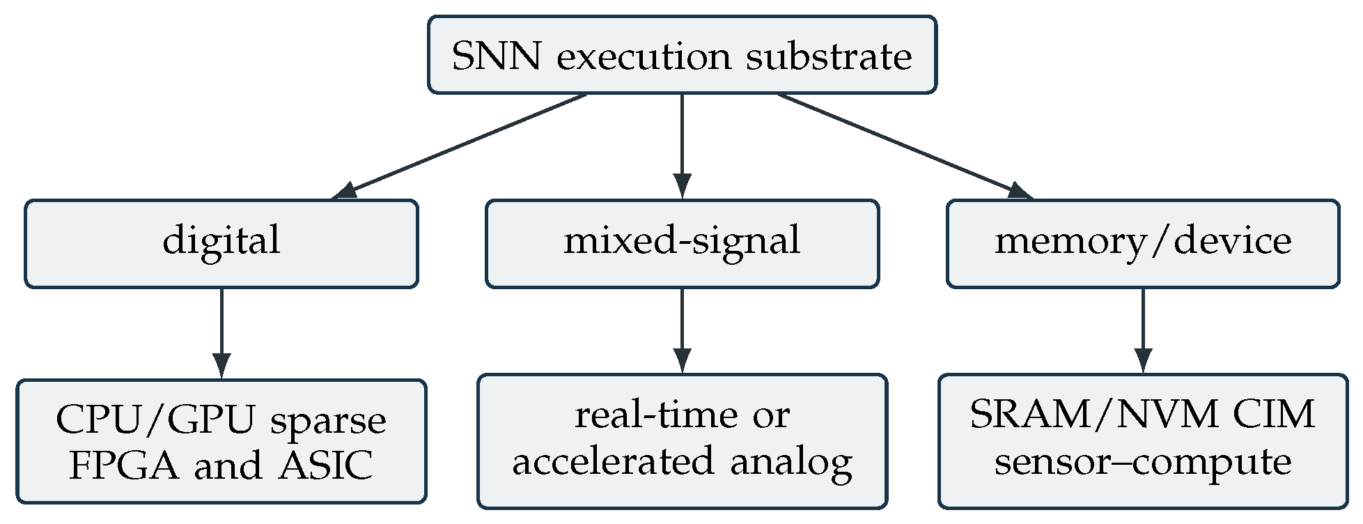
Hardware differs along computation (digital, analog, mixed signal), temporal execution (clocked ticks, globally asynchronous events, accelerated analog time), memory placement, communication, and learning [30,31]. FPGA designs offer inspectable pipelines and custom precision but pay programmable-logic overhead. Digital ASICs give deterministic deployment and scalable routing. Mixed-signal systems realize dynamics physically but require calibration. Compute-in-memory collapses weight storage and accumulation, yet device variability, writes, ADC/DAC, and peripheral circuits can dominate.

Figure 6. Hardware taxonomy. The decisive question is how event communication, state retention, weight access, and time evolution are physically realized.

Figure 6. Hardware taxonomy. The decisive question is how event communication, state retention, weight access, and time evolution are physically realized.

For an event core, $E_{\mathrm{event}}=E_{\mathrm{router}}+k(E_{\mathrm{weight}}+E_{\mathrm{accumulate}})+E_{\mathrm{neuron}}$, where k is delivered fan-out. This equation explains why neuron-update energy alone is not a portable figure of merit.

10. Neuromorphic Chips and Systems

System scale does not follow neuron count alone. Synaptic capacity, reachable fan-in/out, delay storage, weight sharing, link bandwidth, host interface, and real-time deadline determine the largest useful model. On-chip learning further consumes trace memory, update bandwidth, and verification effort. Cross-platform application studies and roadmaps emphasize that software, mapping, and workload fit are system-level constraints [32,33]. Commercial adoption therefore depends as much on stable APIs and ordinary interfaces as on core efficiency [2].

Table 9. Representative platforms, compared by architectural contract rather than a single energy number.

Platform	Compute/time	State and memory	Communication	Learning	Main strength	Main constraint	Evidence
TrueNorth	digital, ticked	distributed core SRAM	event multicast mesh	offline	large deterministic inference fabric	restricted neuron/weights	silicon and application power [3]
Loihi/2 [32,34]	digital, asynchronous/ticked processes	core-local synaptic/neuron state	packet NoC	programmable local learning	flexible dynamics and adaptation	research access and target-specific mapping	chip/system studies
SpiNNaker/2 [35]	programmable many-core	local/external memory	multicast packets	software/accelerators	flexible real-time models at scale	instruction and memory traffic	system studies
BrainScaleS-2 [36]	accelerated mixed signal	analog state plus digital control	event network	hybrid plasticity processors	fast physical dynamics	calibration and finite analog resources	measured hardware [37]
DYNAP family [38]	subthreshold mixed signal	local analog neuron/synapse state	asynchronous AER	local plasticity variants	always-on real-time dynamics	mismatch and capacity	chip papers
Tianjic [39]	digital hybrid ANN/SNN	core-local resources	reconfigurable fabric	mainly offline	hybrid model execution	distinct programming semantics	chip and robot demo
Darwin3	digital ISA-based	compressed connections	mesh routing	programmable on-chip	neuron/learning flexibility and connectivity compression	emerging ecosystem	silicon paper [40]
Speck	asynchronous sensor-compute	on-chip convolution/neuron state	event pipeline	offline deployment	integrated event vision path	application-specific capacity	sensor-chip paper [41]
Akida/Xylo/Innatera	commercial edge families	platform-specific	event/local fabrics	offline plus selected adaptation	product integration and low-power niches	disclosure and cross-platform comparability	datasheet plus task papers
FPGA SNNs	configurable digital	BRAM/URAM/external DRAM	custom NoC/pipeline	usually offline	precision and architecture exploration	lower density/efficiency than ASIC	board measurements

Table 9. Representative platforms, compared by architectural contract rather than a single energy number.

Platform	Compute/time	State and memory	Communication	Learning	Main strength	Main constraint	Evidence
TrueNorth	digital, ticked	distributed core SRAM	event multicast mesh	offline	large deterministic inference fabric	restricted neuron/weights	silicon and application power [3]
Loihi/2 [32,34]	digital, asynchronous/ticked processes	core-local synaptic/neuron state	packet NoC	programmable local learning	flexible dynamics and adaptation	research access and target-specific mapping	chip/system studies
SpiNNaker/2 [35]	programmable many-core	local/external memory	multicast packets	software/accelerators	flexible real-time models at scale	instruction and memory traffic	system studies
BrainScaleS-2 [36]	accelerated mixed signal	analog state plus digital control	event network	hybrid plasticity processors	fast physical dynamics	calibration and finite analog resources	measured hardware [37]
DYNAP family [38]	subthreshold mixed signal	local analog neuron/synapse state	asynchronous AER	local plasticity variants	always-on real-time dynamics	mismatch and capacity	chip papers
Tianjic [39]	digital hybrid ANN/SNN	core-local resources	reconfigurable fabric	mainly offline	hybrid model execution	distinct programming semantics	chip and robot demo
Darwin3	digital ISA-based	compressed connections	mesh routing	programmable on-chip	neuron/learning flexibility and connectivity compression	emerging ecosystem	silicon paper [40]
Speck	asynchronous sensor-compute	on-chip convolution/neuron state	event pipeline	offline deployment	integrated event vision path	application-specific capacity	sensor-chip paper [41]
Akida/Xylo/Innatera	commercial edge families	platform-specific	event/local fabrics	offline plus selected adaptation	product integration and low-power niches	disclosure and cross-platform comparability	datasheet plus task papers
FPGA SNNs	configurable digital	BRAM/URAM/external DRAM	custom NoC/pipeline	usually offline	precision and architecture exploration	lower density/efficiency than ASIC	board measurements

11. Event Sensors and In-Sensor Intelligence

An event camera emits $e_k=(x_k,y_k,t_k,p_k)$ when log intensity changes beyond a polarity-dependent threshold [42]. This suppresses static redundancy and reduces sensing latency, but introduces background activity, threshold mismatch, timestamp bandwidth, and motion-dependent observability. Event cochleae and delta-modulating biomedical front ends offer analogous change-driven streams.

Figure 7. A sensor-to-action loop. Sensor bias, event filtering, I/O arbitration, inference, and feedback belong to the deployed system and its energy/latency boundary.

Figure 7. A sensor-to-action loop. Sensor bias, event filtering, I/O arbitration, inference, and feedback belong to the deployed system and its energy/latency boundary.

In-sensor computing reduces I/O when early features or decisions are formed near pixels or channels. It also couples model updates to sensor calibration and makes privacy/security failures physical: flicker, electromagnetic interference, and crafted motion can perturb event timing. The strongest SNN use case is therefore not merely low average power, but sparse streaming input, persistent temporal state, a hard response deadline, and limited communication to a host.

12. An End-to-End Deployment Pipeline

Deployment proceeds through requirements, representation, training, lowering, mapping, calibration, integration, and monitoring. Requirements fix deadline, duty cycle, accuracy metric, adaptation policy, sensor interface, memory, and energy boundary before model selection. The trained artifact must record neuron equations, time constants, reset, decoder, and preprocessing. Quantization should include weights, membrane, traces, thresholds, and accumulators. Mapping then checks fan-in/out, SRAM, delays, multicast, route congestion, and host fallbacks.

Table 10. Deployment gates and acceptance evidence.

Gate	Artifact	Required test	Reject when	Recovery
Task contract	workload and deadline	representative streams	benchmark omits operating regime	recollect/re-split data
Model contract	equations and decoder	float reference replay	ambiguous reset/time base	canonicalize model
Training	checkpoint and logs	accuracy, firing, early-exit distribution	dense or unstable activity	sparsity/state regularization
Lowering	quantized IR	layer-wise equivalence	unsupported op or overflow	rewrite/retrain
Mapping	placement/routes	capacity and congestion simulation	relay/routing explosion	repartition/architecture change
Hardware	configuration/calibration	trace replay and drift sweep	unacceptable mismatch	hardware-aware fine-tune
Integration	sensor-host-board system	signal-to-decision latency/energy	hidden host bottleneck	move preprocessing/decoder
Operation	telemetry policy	temperature, drift, fault and update tests	unbounded degradation	recalibrate/rollback

Table 10. Deployment gates and acceptance evidence.

Gate	Artifact	Required test	Reject when	Recovery
Task contract	workload and deadline	representative streams	benchmark omits operating regime	recollect/re-split data
Model contract	equations and decoder	float reference replay	ambiguous reset/time base	canonicalize model
Training	checkpoint and logs	accuracy, firing, early-exit distribution	dense or unstable activity	sparsity/state regularization
Lowering	quantized IR	layer-wise equivalence	unsupported op or overflow	rewrite/retrain
Mapping	placement/routes	capacity and congestion simulation	relay/routing explosion	repartition/architecture change
Hardware	configuration/calibration	trace replay and drift sweep	unacceptable mismatch	hardware-aware fine-tune
Integration	sensor-host-board system	signal-to-decision latency/energy	hidden host bottleneck	move preprocessing/decoder
Operation	telemetry policy	temperature, drift, fault and update tests	unbounded degradation	recalibrate/rollback

Simulation-to-hardware equivalence should be checked progressively: spike raster distance, membrane trace error, layer output divergence, final task metric, then closed-loop behavior. Hardware-aware and hardware-in-the-loop training can compensate mixed-signal mismatch [37,43,44,45], but per-device calibration cost must be reported.

13. Evaluation: Accuracy Is One Coordinate

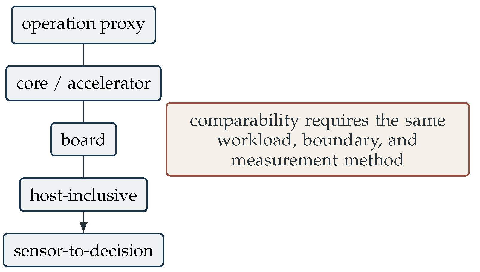
Five evidence boundaries prevent false comparisons: operation proxy, core/accelerator, board, host-inclusive, and sensor-to-decision [1,46]. Let a measurement interval process N samples with baseline power $P_0$ and trace $P\left(t\right)$. Then

$$E_{\mathrm{sample}}={\displaystyle \frac{1}{N}}{\int }_0^{T_m}[P\left(t\right)-P_{\mathrm{excluded}}]dt,$$

(15)

where every excluded component must be named. Report latency distribution, throughput at a stated concurrency, energy per decision, memory footprint, event rate per layer, synaptic deliveries, utilization, temperature, and accuracy. Energy-delay product is useful only after the same system boundary is established.

Figure 8. Evidence ladder. Moving downward includes more real cost but also more platform-specific integration. Operation estimates and measured system energy must not share one ranking column.

Figure 8. Evidence ladder. Moving downward includes more real cost but also more platform-specific integration. Operation estimates and measured system energy must not share one ranking column.

NeuroBench supplies a shared algorithm/system methodology [1]; it does not remove the need to disclose idle subtraction, host work, batching, preprocessing, and timestamp handling. A Pareto set over error, energy, deadline misses, memory, and adaptation cost is more honest than a single score.

14. Applications and Fit Conditions

Neuromorphic SLAM illustrates a good fit because sensing and state estimation are temporal and closed loop [47]. Biomedical spike processing can reduce continuous radio or host traffic [48], but clinical utility, patient shift, and sensor front-end energy matter more than isolated classifier accuracy. Large language SNNs demonstrate optimization scale [49]; without a compatible memory system and measured execution, they do not yet establish an energy advantage.

Table 11. Application fit is determined by input sparsity, state, deadline, and deployment boundary.

Domain	Native event opportunity	Useful SNN state	Deployment value	Main competitor	Missing evidence
Event vision	polarity events	motion/time surfaces	low-latency sparse perception	event ANN on GPU/NPU	full camera-to-output energy
Always-on audio	cochlear/delta events	multiscale filters	sub-mW wake/keyword detection	DSP/TinyML CNN	common front end and noise tests
Robotics	vision, tactile, proprioceptive events	recurrence/control memory	deadline and online adaptation	MCU/GPU controllers	long closed-loop field trials
Biomedical	ECG/EEG/neural events	patient temporal patterns	wearable implant power	DSP and compact RNN	prospective robustness/privacy
Industrial IoT	vibration/change events	anomaly history	communication avoidance	TinyML anomaly models	drift and maintenance cost
Optimization	internally generated events	constraint dynamics	asynchronous search	CPU/GPU solvers	solution quality at equal wall time
Language/generation	token stream	recurrent state	possible binary activation	efficient Transformer/RNN	target hardware and total memory
Scientific simulation	neural spikes	biological dynamics	real-time/accelerated emulation	HPC simulators	model fidelity per energy

Table 11. Application fit is determined by input sparsity, state, deadline, and deployment boundary.

Domain	Native event opportunity	Useful SNN state	Deployment value	Main competitor	Missing evidence
Event vision	polarity events	motion/time surfaces	low-latency sparse perception	event ANN on GPU/NPU	full camera-to-output energy
Always-on audio	cochlear/delta events	multiscale filters	sub-mW wake/keyword detection	DSP/TinyML CNN	common front end and noise tests
Robotics	vision, tactile, proprioceptive events	recurrence/control memory	deadline and online adaptation	MCU/GPU controllers	long closed-loop field trials
Biomedical	ECG/EEG/neural events	patient temporal patterns	wearable implant power	DSP and compact RNN	prospective robustness/privacy
Industrial IoT	vibration/change events	anomaly history	communication avoidance	TinyML anomaly models	drift and maintenance cost
Optimization	internally generated events	constraint dynamics	asynchronous search	CPU/GPU solvers	solution quality at equal wall time
Language/generation	token stream	recurrent state	possible binary activation	efficient Transformer/RNN	target hardware and total memory
Scientific simulation	neural spikes	biological dynamics	real-time/accelerated emulation	HPC simulators	model fidelity per energy

15. Trustworthiness, Reliability, and Lifecycle Risk

SNN failure propagates through timing as well as value. Sensor background activity can cause event floods; dropped packets and timestamp jitter change temporal codes; quantization shifts thresholds; analog mismatch alters time constants; permanent faults remove neurons or links; adversarial perturbations exploit spatial, polarity, and timing channels. Online learning adds poisoning and catastrophic drift.

Table 12. Threats and cross-layer controls.

Threat	Observable	Control
Event flood/spoof	rate/polarity shift	refractory filters, quotas
Timing jitter/drop	latency/raster divergence	sequence numbers, robust code
Weight/state fault	firing imbalance	ECC, redundancy, health tests
Analog drift	parameter/accuracy drift	calibration, noise-aware training
Adversarial events	confidence with sparse edits	temporal augmentation, detection
Learning poisoning	update/trace anomaly	bounded updates, rollback
Side channel	event-dependent power/timing	traffic shaping, isolation
Compiler mismatch	reference-target divergence	differential trace testing

Table 12. Threats and cross-layer controls.

Threat	Observable	Control
Event flood/spoof	rate/polarity shift	refractory filters, quotas
Timing jitter/drop	latency/raster divergence	sequence numbers, robust code
Weight/state fault	firing imbalance	ECC, redundancy, health tests
Analog drift	parameter/accuracy drift	calibration, noise-aware training
Adversarial events	confidence with sparse edits	temporal augmentation, detection
Learning poisoning	update/trace anomaly	bounded updates, rollback
Side channel	event-dependent power/timing	traffic shaping, isolation
Compiler mismatch	reference-target divergence	differential trace testing

Safety cases need operating envelopes for event rate, temperature, supply, missing sensors, and deadline misses. A robust average accuracy does not bound closed-loop hazard. The deployment artifact should therefore include calibration provenance, compiler version, fault tests, monitored statistics, and a rollback path.

16. Cross-Layer Research Agenda

Semantic portability. Continuous-time model definitions need verified discretizations, reset semantics, delay transformations, and precision contracts. NIR is a concrete foundation [5]; conformance suites should compare traces and task outputs across backends.

Sparse training. Current GPU training often unrolls dense time tensors. Event-sparse automatic differentiation, reversible state, checkpointing, and forward/local credit should be evaluated by total training energy as well as inference quality.

Compiler and architecture co-design. Architecture search must ingest measured routing, state, and I/O models. Compilers need traffic-aware partitioning, multicast scheduling, verified fallbacks, and debuggable intermediate states.

Benchmark maturity. Each result should publish event statistics, window policy, precision, mapping, host work, power trace method, idle treatment, and uncertainty. Native event tasks and closed-loop workloads should complement converted image datasets.

Deployment and maintenance. Mixed-signal calibration, per-device variation, secure online learning, telemetry, rollback, and end-of-life updates remain underdeveloped. Neuromorphic roadmaps identify software, benchmarking, and scale as connected adoption problems [2,31].

Application selection. SNNs should compete where temporal state and sparse streaming are intrinsic. On dense offline workloads, efficient ANNs, state-space models, and conventional accelerators remain necessary baselines.

Figure 9. The next bottleneck is not a single neuron or chip. Progress requires semantic, compiler, measurement, and lifecycle maturity to advance together.

Figure 9. The next bottleneck is not a single neuron or chip. Progress requires semantic, compiler, measurement, and lifecycle maturity to advance together.

17. Conclusion

SNNs are best understood as stateful event systems. Their value does not reside in the spike symbol itself, but in whether a complete implementation avoids unnecessary sensing, movement, arithmetic, and synchronization while retaining the temporal information needed by the task. The event contract developed in this survey makes that requirement explicit across semantics, time, state, precision, locality, adaptation, and evidence boundary.

This perspective changes how models and hardware should be judged. A high-accuracy SNN with dense input, long unrolling, analog residual paths, and host-side operators may offer little deployment advantage. A smaller recurrent network paired with an event sensor and local state can be more compelling even when its benchmark accuracy is unremarkable. Likewise, neuron count and synaptic operations do not characterize a chip without routing, memory, supported dynamics, learning, I/O, and software.

The field now has strong ingredients: practical gradient training, local and exact alternatives, deep temporal architectures, interoperable representations, diverse neuromorphic substrates, integrated sensors, and community benchmarking. The unresolved work lies between them. Verified lowering, traffic-aware mapping, comparable system measurement, robust calibration, and lifecycle engineering will decide whether temporal sparsity survives from signal to silicon.

References

- Yik, J.; Ahmed, S.H.; Ahmed, Z.; et al. The NeuroBench Framework for Benchmarking Neuromorphic Computing Algorithms and Systems. Nat. Commun. 2025, 16, 1545. [Google Scholar] [CrossRef] [PubMed]
- Muir, D.R.; Sheik, S. The Road to Commercial Success for Neuromorphic Technologies. Nat. Commun. 2025, 16, 3586. [Google Scholar] [CrossRef] [PubMed]
- Merolla, P.A.; Arthur, J.V.; Alvarez-Icaza, R.; et al. A Million Spiking-Neuron Integrated Circuit with a Scalable Communication Network and Interface. Science 2014, 345, 668–673. [Google Scholar] [CrossRef] [PubMed]
- Gerstner, W.; Kistler, W.M.; Naud, R.; Paninski, L. Neuronal Dynamics; Cambridge University Press, 2014. [Google Scholar] [CrossRef]
- Pedersen, J.E.; Abreu, S.; Jobst, M.; et al. Neuromorphic Intermediate Representation: A Unified Instruction Set for Interoperable Brain-Inspired Computing. Nat. Commun. 2024, 15, 8122. [Google Scholar] [CrossRef] [PubMed]
- Hodgkin, A.L.; Huxley, A.F. A Quantitative Description of Membrane Current and Its Application to Conduction and Excitation in Nerve. J. Physiol. 1952, 117, 500–544. [Google Scholar] [CrossRef] [PubMed]
- Izhikevich, E.M. Simple Model of Spiking Neurons. IEEE Trans. Neural Netw. 2003, 14, 1569–1572. [Google Scholar] [CrossRef] [PubMed]
- Brette, R.; Gerstner, W. Adaptive Exponential Integrate-and-Fire Model as an Effective Description of Neuronal Activity. J. Neurophysiol. 2005, 94, 3637–3642. [Google Scholar] [CrossRef] [PubMed]
- qiang Bi, G.; ming Poo, M. Synaptic Modifications in Cultured Hippocampal Neurons: Dependence on Spike Timing, Synaptic Strength, and Postsynaptic Cell Type. J. Neurosci. 1998, 18, 10464–10472. [Google Scholar] [CrossRef] [PubMed]
- Guetig, R.; Sompolinsky, H. The Tempotron: A Neuron That Learns Spike Timing-Based Decisions. Nat. Neurosci. 2006, 9, 420–428. [Google Scholar] [CrossRef] [PubMed]
- Lee, J.H.; Delbruck, T.; Pfeiffer, M. Training Deep Spiking Neural Networks Using Backpropagation. Front. Neurosci. 2016, 10, 508. [Google Scholar] [CrossRef] [PubMed]
- Zenke, F.; Ganguli, S. SuperSpike: Supervised Learning in Multilayer Spiking Neural Networks. Neural Comput. 2018, 30, 1514–1541. [Google Scholar] [CrossRef] [PubMed]
- Neftci, E.O.; Mostafa, H.; Zenke, F. Surrogate Gradient Learning in Spiking Neural Networks. IEEE Signal Process. Mag. 2019, 36, 51–63. [Google Scholar] [CrossRef]
- Diehl, P.U.; Neil, D.; Binas, J.; Cook, M.; Liu, S.C.; Pfeiffer, M. Fast-Classifying, High-Accuracy Spiking Deep Networks Through Weight and Threshold Balancing. In Proceedings of the International Joint Conference on Neural Networks, 2015. [Google Scholar] [CrossRef]
- Rueckauer, B.; Lungu, I.A.; Hu, Y.; Pfeiffer, M.; Liu, S.C. Conversion of Continuous-Valued Deep Networks to Efficient Event-Driven Networks for Image Classification. Front. Neurosci. 2017, 11, 682. [Google Scholar] [CrossRef] [PubMed]
- Sengupta, A.; Ye, Y.; Wang, R.; Liu, C.; Roy, K. Going Deeper in Spiking Neural Networks: VGG and Residual Architectures. Front. Neurosci. 2019, 13, 95. [Google Scholar] [CrossRef] [PubMed]
- Wunderlich, T.C.; Pehle, C. Event-Based Backpropagation Can Compute Exact Gradients for Spiking Neural Networks. Sci. Rep. 2021, 11, 12829. [Google Scholar] [CrossRef] [PubMed]
- Bellec, G.; Scherr, F.; Hajek, E.; Salaj, D.; Legenstein, R.; Maass, W. A Solution to the Learning Dilemma for Recurrent Networks of Spiking Neurons. Nat. Commun. 2020, 11, 3625. [Google Scholar] [CrossRef] [PubMed]
- Yin, B.; Corradi, F.; Bohte, S.M. Accurate Online Training of Dynamical Spiking Neural Networks through Forward Propagation Through Time. Nat. Mach. Intell. 2023, 5, 518–527. [Google Scholar] [CrossRef]
- Maass, W.; Natschlaeger, T.; Markram, H. Real-Time Computing Without Stable States: A New Framework for Neural Computation Based on Perturbations. Neural Comput. 2002, 14, 2531–2560. [Google Scholar] [CrossRef] [PubMed]
- Zhou, Z.; Zhu, Y.; He, C.; Wang, Y.; Yan, S.; Tian, Y.; Yuan, L. Spikformer: When Spiking Neural Network Meets Transformer. 2023, 2209.15425. [Google Scholar]
- Yao, M.; Hu, J.; Hu, T.; Xu, Y.; Zhou, Z.; Tian, Y.; Xu, B.; Li, G. Spike-Driven Transformer V2: Meta Spiking Neural Network Architecture Inspiring the Design of Next-Generation Neuromorphic Chips. In Proceedings of the International Conference on Learning Representations, 2024. [Google Scholar]
- Orchard, G.; Jayawant, A.; Cohen, G.K.; Thakor, N. Converting Static Image Datasets to Spiking Neuromorphic Datasets Using Saccades. Front. Neurosci. 2015, 9, 437. [Google Scholar] [CrossRef] [PubMed]
- Li, H.; Liu, H.; Ji, X.; Li, G.; Shi, L. CIFAR10-DVS: An Event-Stream Dataset for Object Classification. Front. Neurosci. 2017, 11, 309. [Google Scholar] [CrossRef] [PubMed]
- Cramer, B.; Stradmann, Y.; Schemmel, J.; Zenke, F. The Heidelberg Spiking Data Sets for the Systematic Evaluation of Spiking Neural Networks. IEEE Trans. Neural Netw. Learn. Syst. 2022, 33, 2744–2757. [Google Scholar] [CrossRef] [PubMed]
- Stimberg, M.; Brette, R.; Goodman, D.F.M. Brian 2, an Intuitive and Efficient Neural Simulator. eLife 2019, 8, e47314. [Google Scholar] [CrossRef] [PubMed]
- Eshraghian, J.K.; Ward, M.; Neftci, E.; et al. Training Spiking Neural Networks Using Lessons From Deep Learning. Proc. IEEE 2023, 111, 1016–1054. [Google Scholar] [CrossRef]
- Davison, A.P.; Brüderle, D.; et al. PyNN: A Common Interface for Neuronal Network Simulators. Front. Neuroinformatics 2009, 2, 11. [Google Scholar] [CrossRef] [PubMed]
- Rasmussen, D. NengoDL: Combining Deep Learning and Neuromorphic Modelling Methods. Neuroinformatics 2019, 17, 611–628. [Google Scholar] [CrossRef] [PubMed]
- Roy, K.; Jaiswal, A.; Panda, P. Towards Spike-Based Machine Intelligence with Neuromorphic Computing. Nature 2019, 575, 607–617. [Google Scholar] [CrossRef] [PubMed]
- Christensen, D.V.; Dittmann, R.; Linares-Barranco, B.; et al. 2022 Roadmap on Neuromorphic Computing and Engineering. Neuromorphic Comput. Eng. 2022, 2, 022501. [Google Scholar] [CrossRef]
- Davies, M.; Wild, A.; Orchard, G.; et al. Advancing Neuromorphic Computing With Loihi: A Survey of Results and Outlook. Proc. IEEE 2021, 109, 911–934. [Google Scholar] [CrossRef]
- Schuman, C.D.; Kulkarni, S.R.; Parsa, M.; et al. Opportunities for Neuromorphic Computing Algorithms and Applications. Nat. Comput. Sci. 2022, 2, 10–19. [Google Scholar] [CrossRef] [PubMed]
- Davies, M.; Srinivasa, N.; Lin, T.H.; et al. Loihi: A Neuromorphic Manycore Processor with On-Chip Learning. IEEE Micro 2018, 38, 82–99. [Google Scholar] [CrossRef]
- Furber, S.B.; Galluppi, F.; Temple, S.; Plana, L.A. The SpiNNaker Project. Proc. IEEE 2014, 102, 652–665. [Google Scholar] [CrossRef]
- Pehle, C.; Billaudelle, S.; Cramer, B.; et al. The BrainScaleS-2 Accelerated Neuromorphic System With Hybrid Plasticity. Front. Neurosci. 2022, 16, 795876. [Google Scholar] [CrossRef] [PubMed]
- Gruebl, A.; Billaudelle, S.; Cramer, B.; Karasenko, V.; Schemmel, J. Verification and Design Methods for the BrainScaleS Neuromorphic Hardware System. J. Signal Process. Syst. 2020, 92, 1277–1292. [Google Scholar] [CrossRef]
- Moradi, S.; Qiao, N.; Stefanini, F.; Indiveri, G. A Scalable Multicore Architecture With Heterogeneous Memory Structures for Dynamic Neuromorphic Asynchronous Processors. IEEE Trans. Biomed. Circuits Syst. 2018, 12, 106–122. [Google Scholar] [CrossRef] [PubMed]
- Pei, J.; Deng, L.; Song, S.; et al. Towards Artificial General Intelligence with Hybrid Tianjic Chip Architecture. Nature 2019, 572, 106–111. [Google Scholar] [CrossRef] [PubMed]
- Liu, Y.; et al. Darwin3: A Large-Scale Neuromorphic Chip with a Novel ISA and On-Chip Learning. Sci. Adv. 2024, 10. [Google Scholar] [CrossRef]
- Yousefzadeh, A.; et al. Spike-Based Dynamic Computing with Asynchronous Sensing-Computing Neuromorphic Chip. Nat. Commun. 2024, 15. [Google Scholar] [CrossRef] [PubMed]
- Lichtsteiner, P.; Posch, C.; Delbruck, T. A 128x128 120 dB 15 us Latency Asynchronous Temporal Contrast Vision Sensor. IEEE J. Solid-State Circuits 2008, 43, 566–576. [Google Scholar] [CrossRef]
- Buechel, J.; Zendrikov, D.; Solinas, S.; Indiveri, G.; Muir, D.R. Supervised Training of Spiking Neural Networks for Robust Deployment on Mixed-Signal Neuromorphic Processors. Sci. Rep. 2021, 11. [Google Scholar] [CrossRef] [PubMed]
- Cramer, B.; Billaudelle, S.; Kanya, S.; et al. Surrogate Gradients for Analog Neuromorphic Computing. Proc. Natl. Acad. Sci. 2022, 119, e2109194119. [Google Scholar] [CrossRef] [PubMed]
- Cakal, U.; Wu, C.; Ulusoy, I.; Muir, D.R. Gradient-Descent Hardware-Aware Training and Deployment for Mixed-Signal Neuromorphic Processors. Neuromorphic Comput. Eng. 2024, 4, 014011. [Google Scholar] [CrossRef]
- Ostrau, C.; Klarhorst, C.; Thies, M.; Rueckert, U. Benchmarking Neuromorphic Hardware and Its Energy Expenditure. Front. Neurosci. 2022, 16, 873935. [Google Scholar] [CrossRef] [PubMed]
- Kreiser, R.; Renner, A.; Sandamirskaya, Y.; Pienroj, P. Pose Estimation and Map Formation with Spiking Neural Networks: Towards Neuromorphic SLAM. In Proceedings of the IEEE/RSJ International Conference on Intelligent Robots and Systems, 2018; pp. 2159–2166. [Google Scholar] [CrossRef]
- Burelo, K.; Ramantani, G.; Indiveri, G.; Sarnthein, J. A Neuromorphic Spiking Neural Network Detects Epileptic High Frequency Oscillations in the Scalp EEG. Sci. Rep. 2022, 12, 1798. [Google Scholar] [CrossRef] [PubMed]
- Zhu, R.J.; Zhao, Q.; Li, G.; Eshraghian, J.K. SpikeGPT: Generative Pre-trained Language Model with Spiking Neural Networks. Transactions on Machine Learning Research, 2024. [Google Scholar]
Disclaimer/Publisher’s Note: The statements, opinions and data contained in all publications are solely those of the individual author(s) and contributor(s) and not of MDPI and/or the editor(s). MDPI and/or the editor(s) disclaim responsibility for any injury to people or property resulting from any ideas, methods, instructions or products referred to in the content. |
© 2026 by the authors. Licensee MDPI, Basel, Switzerland. This article is an open access article distributed under the terms and conditions of the Creative Commons Attribution (CC BY) license (http://creativecommons.org/licenses/by/4.0/).
Copyright: This open access article is published under a Creative Commons CC BY 4.0 license, which permit the free download, distribution, and reuse, provided that the author and preprint are cited in any reuse.