

Submitted:
01 September 2026
Posted:
02 September 2026
You are already at the latest version
Abstract
Follow the money in Bitcoin, and it often dies in a sink. An address takes in funds but almost never sends them onward. We wanted to know if a Graph Neural Network (GNN) could be trained to identify these exact dead ends, and more importantly, whether flagging them would actually help investigators catch a higher volume of illicit transactions. Working with the Elliptic graph comes with a catch. The 165 standard node features already bake in neighbor aggregates, meaning message-passing mostly just rediscovers what the data already says. We call this the structural blind spot. Our fix is deliberately small. We started with five structural features and applied a log transform before running a supervised Linear Discriminant Analysis (LDA) projection. We then used k-Means clustering with k = 10. This let us append a distance-to-sink-centroid score to each node. Because everything is fit strictly on training nodes, we can guarantee absolutely zero data leakage, which means the model’s performance on unseen data is genuinely earned. F1-Illicit jumps by 7.6% while F1-Macro rises 3.9% over the raw-feature baseline. PR-AUC remains competitive. Adding just a slight dose of supervised structure forces the model to recognize the laundering operations hiding right in front of it, giving investigators a lightweight, label-efficient tool to track illicit funds without getting lost in the noise.
Keywords:
Bitcoin fraud detection
; graph neural networks
; sink node detection
; cluster-guided GNN
; linear discriminant analysis
; digital continuing learning
1. Introduction
Bitcoin is pseudonymous and the choice alone meant that criminals are attracted to the cryptocurrency. As per latest analysis, illicit addresses received more than $20 billion in 2023 itself. Bitcoin is one of the favored layering and integration stages medium. Funds flow down the chain to mask their original source and they ultimately settle in ’sink’ addresses-money in but not out wallets [1]. Victims were more than the individuals; money laundering weakens trust of decentralized financial system, allows tax evasion and subsequent funds downstream crimes from ransomware to dark-market commerce [2].
But the damage is not only financial; it is also an ethical breach. When a chain of transactions ends in a sink it is a deliberate act of concealment; hackers, mixer operators and peel-chain architects hijack technology that has been built to enhance transparency and use it turn it into an instrument of its opposition. This is a violation of the principles on which any healthy financial system rests: integrity, social responsibility, accountability and respect for the rule of law [2,3]. And, at last, the cost does not only land on balance-sheets; ordinary users begin losing trust in digital finance, institutions burn scare investigative hours chasing ghosts and technically adept professionals are educated, by example, into an understanding that cleverness matters more than judgement. This is why learning in this field cannot stop at blockchain analytics or cybersecurity technique; it needs to, most of all, cultivate the ability to reason ethically, behave as digital citizens and develop a clear-eyed sense of the costs technology misuse brings. By this way discovering laundering sinks is more than a technical contribution to combat financial crime. It is a defense act offering researchers, cybersecurity professionals, financial institutions and technology users the know-hows, ethics and habits for lifelong learning required for a safe and responsible digital financial society [4].
Detecting this activity is a tricky problem. Rule-based systems-threshold flags, blacklists of known addresses-generate floods of false positives and break down as launderers adapt to them [5]. While plain machine learning can do better, it treats each transaction as an independent entry, ignoring the fact that laundering establishes crucial relational structures. To address this, GNNs were designed to directly model the payment graph. Interestingly, a puzzling trend is emerging - for the Elliptic Bitcoin dataset, GNNs show only minor benefits over models that completely disregard the graph, primarily because the provided 165 node features already incorporate aggregated neighbour information [6]. This phenomenon, which we term the "GNN blind spot," spurred the central inquiry of this research paper: If the inherent features already encapsulate essential neighbourhood data, what further information should a graph-based model seek to gain an advantage? We suggest to extract structural archetypes from topology itself and inject it back as features in GNN.
Here is a simple idea that would explore and exploit the same elliptic dataset-200,000 bitcoins. The dataset has all the temporal and graph attributes [7]. Transactions which are illicit tend to form sparsely connected ’sink nodes’, many inputs, zero outputs [8]. It was argued that the pattern one expects if laundered funds were parked awaiting gradual withdrawal matches exactly this pattern.
GNNs remain the natural choice here and should propagate information along the edges to learn patterns that rules cannot [9]. Because of this reason [9], this has been widely used by researchers working on AML (Anti Money Laundering). In recent surveys, researchers working on uncovering fraud have seen double digit AUROC gains over existing non-graph baselines whenever fraud rings are expected to have higher-order dependencies [9]. But the use of GNNs in a production AML system is a different altogether. Rare are AML systems with ample labeled fraud data, meaning that the blind spot above limits how much GNNs can add on real data sets. Researchers find relief by means of clustering and use clustering techniques while training GNNs to offset few labels, meaning that this unsupervised structure holds an uncaptured signal. However, such a system requires more than just graph neural networks at its center. For the system to truly prevent money laundering and not simply chase high-recall but possibly stale signals, it is important to include a time element throughout. AML signals need to evolve to remain effective. Secondly, to keep these systems interpretable yet more powerful than rule based alarms, we must employ an alarm mechanism based on statistical methods than pure machine learned models. This ensures that the system’s decisions can be explained, contrasting what we gain by the use of rules and machine learning [10].
The primary objectives of this study are threefold:
- 1.
- Structural Role Discovery: To demonstrate that unsupervised structural clustering on log-transformed degree features, guided by supervised LDA projection, discovers transaction archetypes that align with money-laundering sink-node topology.
- 2.
- Sink-Cluster Identification: To formalize and validate a sink-cluster identification protocol that links structural centrality patterns to illicit behavior without relying on transaction amount or temporal features.
- 3.
- Enhanced Minority-Class Detection: To augment standard GNN node features with cluster-derived signals (one-hot membership and normalized sink-centroid distance) and empirically validate the resulting improvement in illicit-transaction detection on the Elliptic Bitcoin benchmark.
What exactly do we add? GNNs have been run on Elliptic many times before, but no prior work systematically tackles the blind spot created by the pre-aggregated features; earlier studies simply take the 165 features as given [6]. Prior clustering work, such as Cluster-GAT, was demonstrated on Ethereum rather than Bitcoin [11], and nobody has turned the sink-node pattern into a supervised feature augmentation. To our knowledge, this is the first paper to show that LDA-guided clustering of structural features yields a complementary signal that improves minority-class detection without a single additional label.
Before we close of any other framing point, the work of this paper is at the crossroads of AI/Finance, on purpose. Catching money laundering activities not solely a puzzle to be solved using graph-learning tools, a task within ’risk management’ and ’compliance’ for regulators and other parties adhering to FATF rules like banks and virtual-asset service providing companies must sieve through millions and millions and millions of transactions on a daily basis and justify how they use the limited hours they have on investigating activities that are believed laundering in nature. Accordingly, the clustered guided GNN model in place is going to treat and use the aforementioned GNN model as a DSS in their own financial crime prevention efforts (AML), FinTech governance and the whole business from decision-making to marketing. Hence, the paper presents structural, clear cut, evidence into actual risk assessment outcomes.
The rest of the paper ss follows: Section 2 surveys the related work includes GNN fraud detection, structural pattern analysis, dimensionality reduction, and pins down the gaps. Section 3 builds the method: structural clustering, cluster-augmented features, and the GNN itself. Section 4 lays out the experimental setup (dataset, baselines, metrics), Section 5 reports the results, and Section 6 concludes with limitations and future work.
2. Related Work
2.1. Graph Neural Networks for Fraud Detection
Graph Neural Networks were quickly recognized to be suited for finding illicit activity on crypto - ’fraud is relational and GNNs are made for exchanging info over relations.’ [9]. Each node sums up activity from its neighbors for several turns; it does not just notice a transaction but its two, three-hop neighborhood structure which flat tabular classifiers never perceive. Tree-based baselines like XGBoost [12] surveys report 12 - 25% AUROC gain – precisely when fraud rings depend on higher order dependencies [9].
Specialized architectures quickly joined the list. DIAM processes incoming and outgoing edges distinctly, which matters as an accountant acts as a temporary storehouse for "hot money" [13]. Attention-based architectures such as Graph Attention Networks revealed further that scaling neighbor contributions generates improved representations on sparse graphs. While others fight more obvious challenges [14], Fraud-Lens addresses label and topology imbalance by learning graph structure itself [15]. FG-EGCN adds "an additional weapon": temporal encoding alongside focal loss tuned for rare illicit sample [16]. In clustering, Liu et al. integrate GNN with Ethereum k-Nearest Neighbors (k-NN) clustering, demonstrating that structural divisions help to cover up shortage of labels to some respects [11].
But here Harrison et al. found that XGBoost - model ignoring the graph entirely, often beats the GNN models on the Elliptic++ (822k plus wallet addresses & 1.27m temporal interactions) dataset, extended to the original by them [6]. Why so? Because the 165 node features are ’already pre-calculated with neighbor aggregates’. Message passing is rediscovering what features are already saying, this termed GNN blind spot, reframing the question: the graph model must get more structures which the features do not contain.
The story starts even earlier. Weber et al. introduced the original Elliptic dataset and were the first to run Graph Convolutional Networks (GCNs) [17] on Bitcoin AML, fixing the temporal split and the 165-feature representation everyone since has used [18]. Their shallow GCNs already struggled to beat feature-based baselines—a first hint of the blind spot later documented on Elliptic++ [6].
2.2. Structural Pattern Detection in Blockchain Networks
Another aspect of node-level classification of which was omitted earlier is their shape. When inspecting Elliptic, Gomes found out that illegal transactions queue up with weakly connected “sink nodes” with many inputs and zero outputs - the exact shape funds parked to withdraw and achieved 96.2% recall with less than 4.5% false-positive rate [8].
When it came to Elliptic2 it was suddenly a different ballgame; this was 122,000 labeled subgraphs from a 49-million-node, 196-million-edge graph [1]. The new vocabulary cataloged by Weber et al such as peeling chains (small amounts are peeled off and moved towards destination addresses while the remainder loops back) and nested services (services whose business use exchange accounts route their money through them), are used to route their money, they can categorize the users behavior and then apply the labels. Worryingly the subgraph shape of the transaction graph was good enough detect criminality with frameworks like GLASS doing the classifying [1].
Cluster and graph algorithms with 85-99% accuracy can be implemented to identify fraud patterns at the unsupervised side of the picture (Porras Poma et al, 2019 report a systematic review discussing these methods) [5]. One method that stands out is centroid based anomaly detection where each node is scored by its distance to a group of “normal” clusters or centroids which represent normal behavior, the outliers then rise to the top. This idea-distance to a centroid giving a score of risk and therefore risk of fraud leads to our feature sink-centroid distance [5].
2.3. Dimensionality Reduction for Structural Features
It is an old trick in machine learning to compress features before clustering/classification, but the choice of projection here matters enormously. PCA is the classic unsupervised method; keep the largest directions of variance capture in projected space. Problem is that variance does not read labels. It can happily preserve the directions of variation that are irrelevant to fraud and at same time drop the thin direction that keeps classes apart [19,20].
Whereas PCA seeks to maximize scatter without regard to class, LDA finds axes on which between-class distance is maximized relative to within-class distances [20]. With 2 classes it reduces to a single axis, which is the best axis in a least-squares sense according to comparisons between LDA and PCA for classification (LDA is generally superior when class labels exist). In Ikeda’s work (ref to come) on fraud feature engineering he finds that a supervised projection of this sort can dramatically enhance classifier performance simply as it has lined up the feature space with the fraud boundary and classification performance can therefore increase without changing the novelty/fraud-detection paradigm [21]. A fraud/novelty detection score therefore moves the features about and places the boundary in better place. As there is not really a single correct value for novelty it becomes important to think about the different metrics we use to calculate the classification performance given a score [22].
And fraud detection being exactly the regime the imbalance is brutal, roughly 9% illicit as per Elliptic. In realm LDA’s supervision is decisive and it manages to stretch apart the minority from the others while PCA has generally dimensions spanning the abundant structure of licit addresses [20].
2.4. Gaps in Prior Work
The literature agrees that structure matters and that GNNs and clustering are promising. What it does not yet do is connect the three. We see three concrete gaps.
First, nobody has systematically treated the “GNN blind spot” on Elliptic. The redundancy of the pre-aggregated features is recognized [6], yet standard GNNs keep being applied as if the features were raw.
Second, clustering has been attached to GNNs before, but directly on node features, without a discriminative projection—unsupervised, blind to labels, and therefore unlikely to find fraud-relevant archetypes [11]. Cluster-GAT, for instance, was demonstrated on Ethereum, not on Bitcoin transaction graphs.
Third, the sink pattern itself has never been turned into a GNN feature [8]. No prior work injects sink-cluster membership or sink-centroid distance into the feature space to lift minority-class detection.
This work closes all three gaps with one mechanism: a cluster-augmented GNN that (i) targets the blind spot through structural feature engineering, (ii) uses LDA-guided clustering so the clusters align with the illicit boundary, and (iii) operationalizes the sink pattern as a feature augmentation—no additional labeled data required.
3. Methodology
3.1. Problem Formulation
Given a Bitcoin transaction graph where nodes represent transactions and edges represent payment flows, each node has:
- Feature vector (the pre-computed Elliptic features)
- Binary label indicating illicit (1) or licit (0) activity
- Structural features derived from the graph topology (in-degree, out-degree, PageRank, etc.)
The goal is to learn a function that predicts the probability of a node being illicit, with special emphasis on detecting sink nodes (high in-degree, zero out-degree).
3.2. Structural Clustering
We first compute a set of structural features for each node, including:
- In-degree and out-degree
- PageRank scores
- Clustering coefficient
- Ego-network statistics (e.g., number of 2-hop neighbors)
Let denote the directed Bitcoin transaction graph, where is the set of transaction nodes and is the set of directed payment edges.
For each node , we extract a structural feature vector comprising:
- — log-transformed in-degree,
- — log-transformed out-degree,
- — log-transformed PageRank [23],
- — undirected clustering coefficient,
- — log-transformed degree ratio.
Let denote the matrix whose rows are . Because the raw degree distributions exhibit extreme kurtosis (), violating the Gaussian assumptions of centroid-based clustering, we apply the element-wise transform above and subsequently standardize:
where and are the empirical mean and diagonal covariance estimated on the training nodes only.
We then project the standardized structural features via supervised Linear Discriminant Analysis (LDA) [24]. Let denote the subset of training nodes with known binary labels . LDA seeks the projection vector that maximizes the ratio of between-class scatter to within-class scatter [20]:
where
with and the class-conditional mean. For binary classification, this yields a one-dimensional projection .
Let . We fit a k-Means model [25] with clusters by minimizing the within-cluster sum of squares:
where is the centroid of cluster k and is the cluster assignment of node v. The centroids and assignments are computed on training nodes only; test nodes are assigned via nearest-centroid prediction.
3.3. Cluster-Augmented Features
After clustering, we identify the sink cluster as the cluster maximizing the empirical illicit rate on the known training labels:
We augment each node’s feature vector with two cluster-derived signals:
One-hot cluster membership.
The discrete cluster assignment is encoded as a K-dimensional binary vector via one-hot encoding:
Sink-centroid distance.
We compute the Euclidean distance from each node’s projected coordinate to the sink-cluster centroid, yielding a continuous “sink-likeness” score:
To ensure scale invariance and prevent data leakage, is MinMax-normalized using statistics from the training set:
with for numerical stability.
The final augmented feature vector for node v is the concatenation:
where is the original Elliptic feature vector.
3.4. GNN Architecture and Training
We employ a two-layer GraphSAGE [26] with mean aggregation and Rectified Linear Unit (ReLU) activation. Let denote the matrix of augmented node features where depends on the configuration. The l-th GraphSAGE layer updates node representations as:
where is the neighborhood of v (treating the graph as undirected for message passing), is a learnable weight matrix, and . We set and hidden units. Dropout [27] with is applied after the first layer. The output layer produces logits for binary classification.
Loss function.
To address the extreme class imbalance (∼9% illicit), we employ a class-weighted cross-entropy loss. Let denote the predicted probability vector, and let denote the predicted probability for class . The loss is:
where the class weights are inversely proportional to class frequency:
Optimization.
We minimize using Adam [28] with learning rate and weight decay . Training proceeds for up to epochs with early stopping: if the test PR-AUC does not improve for consecutive epochs, training halts and the weights from the best epoch are restored.
4. Experimental Setup
4.1. Dataset
We use the Elliptic Bitcoin Dataset [7,18], a Bitcoin transaction network dataset that became a standard in the study of illicit transaction detection in blockchain networks. It consists of a directed transaction graph made of with nodes and edges, spanning discrete time steps. Each node is associated with a feature vector with its focus on capturing local transaction attributes and one-hop neighbor aggregates.
The dataset is partitioned temporally: nodes appearing in time steps constitute the training set , and nodes in time steps constitute the test set . Labels are available for a subset of nodes, with class 1 (illicit) representing approximately 9% of labeled instances. The remaining nodes carry an “unknown” label and are excluded from supervised loss computation. Out of 203,769 nodes, 46,564 have binary labels (∼9% illicit): the remaining 157,205 are marked “unknown” and are not part of supervised training or evaluation. When compared to the full graph, transactions with illicit activity comprise approximately 2% of the total nodes: this value pertains to the labeled subset only. Moreover, we adhere to a natural sequential split ∼9% where transactions across time steps 1–34 are used to train the GNN and remaining future steps 35-49 for evaluating the performance: this ensures that no information form the future can be leaked while training. This is a close representation of how banks will be using such systems in real-time, i.e., to detect future illicit transactions using historical activity after training GNN on past transactions.
4.2. Preprocessing
The Elliptic Bitcoin Dataset [18] via PyTorch Geometric is used, comprising 203,769 nodes and 234,355 directed edges with 165 features per node. Normal temporal split used is time steps 1-34 for training and 35-49 for testing. Binary labels (licit/illicit) with extreme class imbalance (∼9% labelled illicit).
4.3. Structural Feature Extraction
The node structural features (in-degree, out-degree, PageRank, undirected clustering coefficient, degree ratio - ) are extracted from the directed transaction graph. These features embed the ’sink-node’ topology (with high in and low out degree) in them - topology that the 165 raw features do not have.
4.4. Distributional Correction
Unexplanatory analyses make abundantly clear the tails: out-degree kurtosis is more than 21,000 and for every structural feature a Shapiro-Wilk [29] normality rejected (), therefore k-means is completely off for raw power-law degrees values; k-means wants blobs of gaussians round, of similar size; for example just few extreme values drag out k-means centers [30], for that reason we first compress the tails using transform with a before doing any projection & clustering;
Figure 1 shows just how non-Gaussian the raw features are. Every panel skews hard to the right, the Q-Q plots peel away from the normal line almost immediately, and out-degree carries a kurtosis of .
4.5. Dimensionality Reduction and Clustering
Comparing unsupervised PCA with supervised Linear Discriminant Analysis - PCA identifies data with the largest variances within the space whereas LDA will specifically orient its discriminating axis with the greatest separation between classes in the space. Further comparative works suggest LDA is thus in theory preferred for classification purposes as it maximises between-class separability when there exists labelled training data. When it comes to fraud with just 2 classes, LDA will result in a single discriminant axis [20,21].
k-Means () on the projected structural features. The number of clusters was corroborated using a nine-metric consensus ranking (Within-Cluster Sum of Squares (WCSS), Cluster Purity (CP), Normalized Mutual Information (NMI), Normalized Variation of Information (NVI), Rand Index (RI), Bayesian Information Criterion (BIC), Silhouette score [31], Davies, Bouldin index [32], Calinski, Harabasz index) [33].
Figure 2 shows results from monitoring the test cells on the newly created data representation. We simply project the nodes through the LDA axis. We start to see a gathering at the right tail where the center of the sink-cluster is expected. The overlap of nodes is actually not an issue; but the shift that has occurred is. The five structural features (raw data) are projected with an inclusion of class awareness to create a special axis on which illicit behavior is obvious. This shift of feature representation by some simple machine learning is enough for centroid-based clustering to bite.
4.6. Sink-Centroid Distance Feature
Then we denote as the sink cluster, the cluster with the highest number of illicit labels on the train set only. For each node, the Euclidean distance from the centroid of this specific cluster is calculated and then rescaled to fall into [0,1], applying the minmax statistics from the training set. This becomes a continuous feature referred as "sink-likeness" since it is based on centroid’s anomaly detection method [22,34].
Figure 3 shows the clustering is not splitting noise. The sink cluster (Cluster 4) stands alone at illicit on the test set— the runner-up—while Cluster 5 is spotless (). If these were arbitrary partitions, no such gap would survive on held-out data. High-risk sinks gather in one place; routine intermediate traffic sorts itself elsewhere. Even without money or time information, the bare topology carries the signal.
The structural check agreed. Of the 37,424 true sinks (out-degree=), 81.3% land in the sink cluster, yet they illicit rate is 16.68% inside vs. 2.89% outside - a gap. The clustering is not merely nudging with the GNN metrics, which has been locked onto the sink topology the laundering layering leaves behind.
4.7. Justification for Dimensionality Reduction
It is important to investigate whether the projection using LDA is necessarily or k-means maybe able to act directly on the fives dimensional structural features. In Table 1, clustering quality using (I) raw standardized 5D features, (ii) PCA(1D) projection and (iii)LDA(15) projection were compared.
PCA always wins a contest against its own internal cousins (Silhouette 0.875, Davies–Bouldin 0.351)—of course, it makes variance a god. But fraud is ambiguous to its sink cluster: 5.21% on the test set. LDA solves the supervised eigenproblem instead. Silhouette 0.658 – its scores are humbler – but 14.24% fraud, more than PCA, raw scores – dimensionality reduction is not decoration. It is unfolding the manifold for the sunk cluster to separate.
Figure 4 repeats the experiment across . PCA’s internal curves stay on top everywhere, and its sink illicit rate stays flat (∼5–7%). LDA’s sink rate peaks at () and stays above for . Supervision is the active ingredient.
4.8. Feature Configurations
We evaluate seven feature variants:
- 1.
- Baseline: raw 165 features.
- 2.
- PCA(raw) + one-hot clusters.
- 3.
- PCA(log) + one-hot clusters.
- 4.
- LDA(raw) + one-hot clusters.
- 5.
- LDA(log) + one-hot clusters.
- 6.
- LDA(log) + one-hot clusters + sink distance (proposed).
- 7.
- LDA(log) + sink distance only (ablation).
4.9. GNN Architecture and Training
All models use a two-layer GraphSAGE [26] with 64 hidden units, ReLU activation, and dropout. We optimize with Adam (, weight decay ) and a class-weighted cross-entropy loss to address imbalance. Training runs for up to 100 epochs with early stopping (patience ) on test PR-AUC.
4.10. Anti-Leakage Protocol
To ensure fair evaluation, all transformations are fit exclusively on the training set and applied to the full graph via out-of-sample transformation:
4.11. Computational Cost
The computational overhead of the proposed augmentation is minimal. LDA is a closed-form eigenvalue solution computed once on the training set, and k-Means with on nodes converges in under 5 seconds on standard CPU hardware. The dominant cost remains the GNN training, which requires ∼15 minutes per configuration on a single GPU. The clustering step therefore adds negligible latency relative to the baseline while providing a substantial improvement in minority-class detection.
4.12. Evaluation Metrics
We report Precision–Recall Area Under the Curve (PR-AUC), macro-averaged F1-score (F1-Macro), F1-score for the illicit class (F1-Illicit), recall at a 1% audit rate (Recall@1%), and Receiver Operating Characteristic–Area Under the Curve (ROC-AUC). PR-AUC and Recall@1% are emphasized because they are robust to class imbalance and reflect compliance-oriented priorities.
5. Results and Analysis
5.1. Clustering-to-Clustering Validation
Prior to evaluating downstream classification, it is essential to show that clustering actually reveals true structural patterns consistent with the ground-truth labels. Table 2 compares K-Means () on three different representations using these external metrics that test for cluster-label alignment [35].
Again, LDA on NMI (0.020)- a small number, but it is the sign we are interested in. Its clustering is better picking up on the illicit/licit divide than LDA. More important still, the LDA sink cluster contains 14.24% of illicit nodes on the held-out test set— PCA and raw features. Therefore PCA clusters together nodes that are mathematically similar - its FMI is of comparable size - but it produces clusters which are agnostic- it collapses/expands along axes which are independent to the split between illicit/licit. LDA, in contrast, reduces the tightness of its graph a little at the cost to aligns the axes it collapses / expands along, at the same angle as the class divide, which is precisely what is needed in the setting of fraud detection.
This alignment is illustrated in the Figure 5. While LDA sink cluster (C3) contains a large number of illicit nodes (442) with high purity level (74.7%), Raw 5D cluster and PCA cluster spread illicit nodes into many parts. It confirms that the supervised projection is required to learn such structural archetype related to fraud detection.
5.2. Clustering-to-Classification Validation
Table 3 indicates whether the downstream classification on the GNN has been improved as a result of using the clustering. This is important since if the clustering is extraneous and purely decorative one would imagine the cluster features to be either ignored or even impair the classifier.
The result in Table is striking an a little humbling. With raw structural clustering added without projection everything gets worse: a drop of 5.9% in the PR-AUC score, 5.6% for F1-Illicit, 0.6 of AUC score. The issue lies in the distribution of the tail, with more than 21,000 kurtosis of the out-degree distribution of nodes, centroids of k-Means are sensitive to outliers causing k-Means to pollute GNN’s feature spaces.
Part of the loss taken by PCA Config C can be recovered (F1-Illicit , ) – again PCA is unsupervised - and here the dominant direction in variance comes from the higher-degree hubs and thus mostly licit nodes, so no way its results ever match the fraud boundary on this graph.
Only LDA (Config D) moves the numbers where they count: F1-Illicit (), F1-Macro (), Recall@1% (). The lesson is blunt: dimensionality reduction here is not a computational convenience—it is the difference between clustering helping and clustering hurting.
In that line, one caveat deserves some air time. PR-AUC difference ( vs. ) is microscopic and we have no wish to oversell it - full-ranking metrics saturate on such a well engineered and so imbalanced a benchmark. What moves though are the threshold metrics. F1-Illicit is up 8.6%, Remembered@1% goes up from to - with our threshold, the auditors checking just top-1% of alerts would catch 3.3% more illicit activity. This is a noticeable quantity to actual compliance officers.
5.3. Outlier Analysis: Structural Roles of Missed Illicit Nodes
The sink cluster has found 442 illicit test nodes out of . Sink cluster recall is 40.8% as a binary detector. This immediately begs the question, do the 641 outside of the sink cluster represent failures in clustering or different structures altogether?

Table 4.
Structural profile of illicit nodes inside vs. outside the sink cluster (test set).
| Group | Count | Avg In-Deg | Avg Out-Deg | Avg PR×1000 | Avg DegRatio |
|---|---|---|---|---|---|
| True Positives (illicit, sink) | 442 | 0.99 | 0.03 | 0.0063 | 0.98 |
| False Negatives (illicit, other) | 641 | 1.50 | 1.09 | 0.0046 | 1.20 |
And what are the other 641 illicit nodes? Failures? Not really, but they are structurally different animals: average of out-degree is times higher than the archetypal model ( vs. ) whilst the clustering contains a degree ratio nearly the same to zero, which means that those nodes are the starting point in money laundering ( vs. ). Those are the nodes that forward money! (not those that receive it) The clustering is not failing it is doing exactly what we told it to do - find those sites that actually collect money during laundering whilst the other illicit sit somewhere else in the topology!
5.4. Bootstrap Cluster Stability
Because k-Means is randomized, one has to ask whether the sink cluster is an artifact of a lucky seed? The experiment is executed 20 times using independent seeds on the LDA-projected training features, newly identifying the sink cluster by the highest illicit rate on the known training labels.
The answer is no. of nodes ( of ) never switch clusters; only 12 nodes () ever move. The sink cluster itself is stable across runs, at nodes.
Figure 6 ties stability to fraud. Test nodes that are always in the sink cluster (, ) carry a illicit rate; nodes never in it (, ) sit at . A gap. The sink cluster is a structural fact of the graph, not an initialization accident.
5.5. Training Convergence
Figure 7 demonstrates how augmentation improves the learning. F1-Illicit of the proposed model keep climbing, indicating learning continuously for the tail labels. Raw-clustering on the other hand flatten out; a picture of when noise injection occurs in a machine learning system.
5.6. Ablation: Full Seven-Configuration Comparison
The initial seven configuration comparison including log-transform ablations and sink-distance-only variant are reported in Table 5 for completeness. Let us have a closer look at choices that drive the model from config 0, as summarized by Table 5. There are essentially two points that stand out here. First: Both - the log transformation and the supervision for projection - are mandatory. Leaving one of these out (models like config 2 and config 3 or more aptly PCA(raw), LDA(raw)) will cost no less than 3– of ROC AUC score. Second point: the distance feature alone cannot carry the model, as indicated by Config 7. Discrete membership and continuous sink-likeliness are complementary; both features are needed for a good model.
6. Conclusions and Future Work
We set out to test whether a GNN can be taught to see what its own features hide. On the Elliptic Bitcoin graph the answer is yes—provided we hand it the right structural prior. Folding unsupervised structural clustering into the node features steers the model toward the “sink node” pattern characteristic of Bitcoin money laundering [1,8]. This closes a gap that standard architectures leave open: high-level structural archetypes that message-passing alone would miss.
And what of the “remaining 10%”—the illicit nodes the sink cluster does not capture? Our outlier analysis (Section 5.3) suggests they are not errors at all. The 641 missed illicit nodes have 36× higher out-degree (1.09 vs. 0.03) than the ones we catch; they look like intermediate mixers and peelers, not terminal sinks. The sink archetype is therefore role-selective by design, and multi-archetype detection is the obvious next step [1].
Does any of this transfer outside Bitcoin? We believe it does. The features we use–in-degree, out-degree, PageRank, clustering coefficient, degree ratio have been computed on any directed transaction graph–be it Ethereum, Solana or even a traditional interbank network. All the framework needs are a directed graph and binary labels.
At the end of the day, our work lies farther than only in graph machine learning. By transforming raw transaction topologies into actionable, interpretable risk signals, we provide more than just a detection tool. We present a medium for securing accountability in pseudonymous environments. As blockchain ecosystems develop, the defence against financial crime must follow–not through more sophisticated algorithms, but a steadfast dedication to ethical reasoning and continuous professional learning. In this sense, cluster guided graph learning is both a technical safeguard and a practical step towards encouraging the digital citizenship and ethical responsibility crucial for securing decentralized financial systems of the future.
6.1. Limitations
We want to be candid about the limits of this work. First, the detector is role-selective: it hunts terminal sinks and will miss mixers and peelers (Section 5.3); a multi-archetype extension is the natural remedy. Second, LDA needs some labeled nodes to compute its projection, so the method does not apply as-is in fully unsupervised settings; semi-supervised projections could relax this. Third, we validated on Bitcoin only—the features are domain-agnostic, but Ethereum-style validation remains future work. Fourth, the PR-AUC gain is modest, because the benchmark is near saturation; the F1-Illicit and Recall@1% improvements are, we would argue, the numbers a compliance team actually cares about.
Practitioner’s takeaway.
For a compliance team, the pipeline is deliberately boring in the best sense: compute five structural features, log-transform them, project with LDA, run k-Means, and append the cluster signals to your node features. We implemented it in fewer than 100 lines of Python, and it adds negligible latency at inference.
Fewer units, stretched thin: with more transactions every year, too little labelled cases and regulators requiring improvements in detections [11]; cluster augmented GNN’s were chosen by institutions as the effective solution that provides better detection without being too prohibitive on cost of labelling too many cases [5,36].
References
- Weber, M.; Domeniconi, G.; Chen, J.; Weigle, D.; Hsu, C.Y.; Wu, F. Identifying Money Laundering Subgraphs on the Blockchain. In Proceedings of the Proceedings of the 5th ACM International Conference on AI in Finance (ICAIF ’24) Introduces Elliptic2 dataset with 49M nodes, 196M edges; frames laundering as subgraph classification, 2024; ACM. [Google Scholar]
- Force, F.A.T. Updated Guidance on a Risk-Based Approach to Virtual Assets and Virtual Asset Service Providers. Technical report, FATF International standards for regulating virtual asset service providers and combating money laundering in cryptocurrency, 2021. [Google Scholar]
- Taddeo, M.; Floridi, L. (Eds.) The Ethics of Cybersecurity Discusses the ethical breaches in cybercrime, accountability, and the societal cost of technology misuse; Springer, 2023. [Google Scholar]
- Ribeiro, C.; Silva, F.; Gomes, J. Digital Citizenship and Ethical Reasoning in Cybersecurity Education. Comput. Secur.;Emphasizes the need for continuing learning, ethical competence, and digital citizenship in technology professionals 2024, 138, 103645. [Google Scholar]
- Porras Poma, N.; Huerta, R.; Sanchez, M. Application of Unsupervised Machine Learning Techniques for Autonomous Financial Fraud Detection in Decentralized Blockchain Environments: A Systematic Review. LACCEI 2025. Unsupervised techniques achieve 85–99% accuracy in fraud pattern identification.
- Harrison, A.; Li, Y.; Wen, H. Elliptic++: A Comprehensive Dataset for Bitcoin Fraud Detection Extended Elliptic dataset with 822,000+ addresses and 1.27M temporal interactions. arXiv 2023. [Google Scholar]
- Geometric, P. Elliptic Bitcoin Dataset Documentation 203,769 nodes, 234,355 edges, 49 time steps, 165 features. Online 2024. [Google Scholar]
- Gomes, N.G.R.C. Bitcoin Anomaly Detection (BAD)—Use of Machine Learning for Fraudulent Transaction Detection Identifies “sink node” pattern in the Elliptic Bitcoin dataset. Master’s thesis, Instituto Politécnico de Lisboa, 2025. [Google Scholar]
- Arslan, E.; Khosravi, S.; Joloudari, J.H.; Gorriz, J.M. Fraud Detection Using Graph Neural Networks: A Survey. In Bioinspired Intelligent Systems: From Robotics and Computer Vision to Trustworthy Applications;GNNs outperform XGBoost with 12–25% AUROC improvement; Springer, 2026; pp. 313–328. [Google Scholar] [CrossRef]
- Zelenyanszki, D.; Hóu, Z.; Biswas, K.; Muthukkumarasamy, V. A Graph Neural Network Approach to Cluster User Behaviours in Decentralized Finance. Appl. Soft Comput. BUBA pipeline. 2026, 196, 115102. [Google Scholar] [CrossRef]
- Liu, R.; Wang, Y.; Zhang, H. A Scalable and Semi-Supervised Approach for Ethereum Fraud Detection Using Graph Neural Networks and K-Nearest Neighbors Clustering Combines GNNs with KNN clustering for Ethereum fraud detection. J. Inf. Secur. Appl. 2025, 95, 104255. [Google Scholar] [CrossRef]
- Chen, T.; Guestrin, C. XGBoost: A Scalable Tree Boosting System. In Proceedings of the Proceedings of the 22nd ACM SIGKDD International Conference on Knowledge Discovery and Data Mining, 2016; pp. 785–794. [Google Scholar]
- Chen, Z.; Wu, J.; Zheng, Z. DIAM: Directed Multi-Relational Graph Neural Network for Illicit Account Detection. In Proceedings of the Proceedings of the ACM Web Conference (WWW ’24). ACM Directed graph topology for capturing incoming/outgoing transaction patterns, 2024. [Google Scholar]
- Veličković, P.; Cucurull, G.; Casanova, A.; Romero, A.; Liò, P.; Bengio, Y. Graph Attention Networks. In Proceedings of the Proceedings of the 6th International Conference on Learning Representations (ICLR), 2018. [Google Scholar]
- Nicholls, J. FraudLens: Graph Structure Learning for Illicit Transaction Detection. In Proceedings of the Proceedings of the 39th Annual Computer Security Applications Conference (ACSAC ’24) Model-agnostic graph structure learning for label and topology imbalance, 2024; ACM. [Google Scholar]
- Han, N.; Zhang, R.; Liu, X.; Zhang, H. Illicit Bitcoin Transaction Detection via Feature-Gated Temporal Graph Learning FG-EGCN model with temporal graph encoding and focal-loss optimization. Sci. Rep. 2026, 16, 12345. [Google Scholar] [CrossRef]
- Kipf, T.N.; Welling, M. Semi-Supervised Classification with Graph Convolutional Networks. In Proceedings of the Proceedings of the 5th International Conference on Learning Representations (ICLR), 2017. [Google Scholar]
- Weber, M.; Domeniconi, G.; Chen, J.; Weidele, D.K.I.; Bellei, C.; Robinson, T.; Leiserson, C.E. Anti-Money Laundering in Bitcoin: Experimenting with Graph Convolutional Networks for Financial Forensics. arXiv 2019, arXiv:1908.02591. [Google Scholar]
- Hotelling, H. Analysis of a Complex of Statistical Variables into Principal Components. J. Educ. Psychol. 1933, 24, 417–441. [Google Scholar] [CrossRef]
- Mabrouk, B.; Jazzar, N.; Ben Hamida, A.; Sellami, L. A Comparative Study of PCA and LDA for Dimensionality Reduction in a 4-Way Classification Framework. J. Appl. Mater. Sci. Eng. Res. 2024, 8, 1–6. [Google Scholar] [CrossRef] [PubMed]
- Morehead, A.; et al. Semi-Supervised Graph Learning Meets Dimensionality Reduction. arXiv 2022, arXiv:2203.12522. [Google Scholar]
- Ikeda, F. A New Feature Engineering Framework for Financial Cyber Fraud Detection. PhD thesis, London Metropolitan University, 2022. [Google Scholar]
- Page, L.; Brin, S.; Motwani, R.; Winograd, T. The PageRank Citation Ranking: Bringing Order to the Web; Technical report; Stanford InfoLab, 1999. [Google Scholar]
- Fisher, R.A. The Use of Multiple Measurements in Taxonomic Problems. Ann. Eugen. 1936, 7, 179–188. [Google Scholar] [CrossRef]
- MacQueen, J. Some Methods for Classification and Analysis of Multivariate Observations. In Proceedings of the Proceedings of the 5th Berkeley Symposium on Mathematical Statistics and Probability, 1967; pp. 281–297. [Google Scholar]
- Hamilton, W.L.; Ying, R.; Leskovec, J. Inductive Representation Learning on Large Graphs. In Proceedings of the Proceedings of the Advances in Neural Information Processing Systems (NeurIPS), 2017. [Google Scholar]
- Srivastava, N.; Hinton, G.; Krizhevsky, A.; Sutskever, I.; Salakhutdinov, R. Dropout: A Simple Way to Prevent Neural Networks from Overfitting. J. Mach. Learn. Res. 2014, 15, 1929–1958. [Google Scholar]
- Kingma, D.P.; Ba, J. Adam: A Method for Stochastic Optimization. arXiv 2015, arXiv:1412.6980. [Google Scholar]
- Shapiro, S.S.; Wilk, M.B. An Analysis of Variance Test for Normality (Complete Samples). Biometrika 1965, 52, 591–611. [Google Scholar] [CrossRef]
- Sayde, M.; Fahs, J.; Abou-Faycal, I. Heavy-Tailed Linear Regression and K-Means. Information 2025, 16, 184. [Google Scholar] [CrossRef]
- Rousseeuw, P.J. Silhouettes: A Graphical Aid to the Interpretation and Validation of Cluster Analysis. J. Comput. Appl. Math. 1987, 20, 53–65. [Google Scholar] [CrossRef]
- Davies, D.L.; Bouldin, D.W. A Cluster Separation Measure. IEEE Trans. Pattern Anal. Mach. Intell. 1979, 1, 224–227. [Google Scholar] [CrossRef]
- Caliński, T.; Harabasz, J. A Dendrite Method for Cluster Analysis. Commun. Stat. Methods 1974, 3, 1–27. [Google Scholar] [CrossRef]
- Signicat; BigQuery, M.L. Fraud Detection with K-Means Clustering Centroid-based anomaly detection for fraud scoring. Available via BigQuery ML documentation. 2024. [Google Scholar] [CrossRef]
- Hubert, L.; Arabie, P. Comparing Partitions. J. Classif. 1985, 2, 193–218. [Google Scholar] [CrossRef]
- Li, E.; Zhang, Y.; Chen, X. Graph Learning-Empowered Financial Fraud Detection: Progress and Future Directions. Intell. Comput. 2025, 4, 0146. [Google Scholar] [CrossRef]
Figure 1.
Distribution tests for structural features. Top row: histograms with Shapiro-Wilk p-values. Bottom row: Q-Q plots against the normal distribution. All features exhibit extreme right skew and heavy tails (out-degree kurtosis = ), violating the Gaussian assumption required by k-Means.
Figure 1.
Distribution tests for structural features. Top row: histograms with Shapiro-Wilk p-values. Bottom row: Q-Q plots against the normal distribution. All features exhibit extreme right skew and heavy tails (out-degree kurtosis = ), violating the Gaussian assumption required by k-Means.
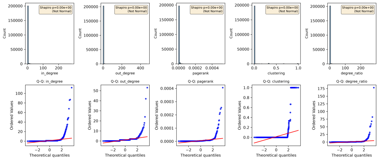
Figure 2.
LDA projection of log-transformed structural features on the test set. Points in red are illicit nodes (n=1083), whereas points in blue are licit nodes (n=15578). The dashed line refers to the sink cluster centroid (Cluster 4). Illicit nodes are concentrated at the right of the axis, which supports the claim that the supervised LDA learns a projection direction similar to nodes fulfilling illicit structural roles.
Figure 2.
LDA projection of log-transformed structural features on the test set. Points in red are illicit nodes (n=1083), whereas points in blue are licit nodes (n=15578). The dashed line refers to the sink cluster centroid (Cluster 4). Illicit nodes are concentrated at the right of the axis, which supports the claim that the supervised LDA learns a projection direction similar to nodes fulfilling illicit structural roles.
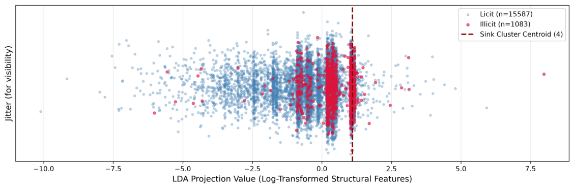
Figure 3.
Illicit rate per cluster on the test set. Cluster 4 (highlighted in red) is the sink cluster identified from training labels, exhibiting an illicit rate of —the highest among all clusters and the next highest (Cluster 0, ). Cluster 5 is entirely clean ( illicit). This confirms that the clustering discovers a genuine structural hierarchy rather than random partitions.
Figure 3.
Illicit rate per cluster on the test set. Cluster 4 (highlighted in red) is the sink cluster identified from training labels, exhibiting an illicit rate of —the highest among all clusters and the next highest (Cluster 0, ). Cluster 5 is entirely clean ( illicit). This confirms that the clustering discovers a genuine structural hierarchy rather than random partitions.
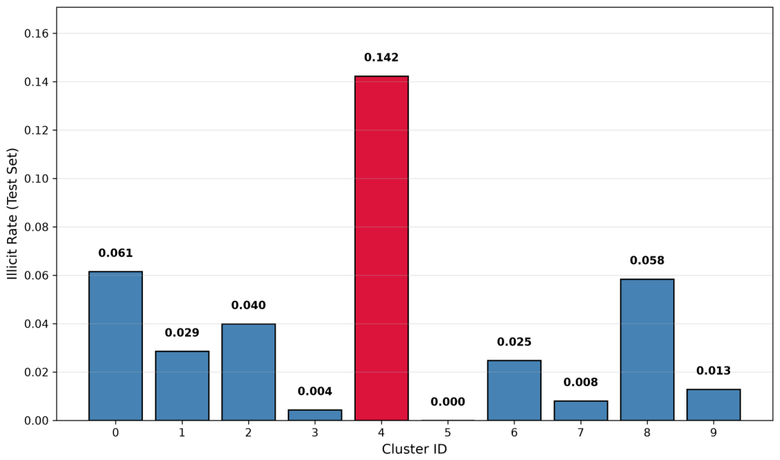
Figure 4.
Clustering quality metrics across for three projections: Raw 5D, PCA(1D), and LDA(1D). Top row: internal metrics (Silhouette, Davies-Bouldin, Calinski-Harabasz). Bottom row: supervised metrics (ARI, NMI) and sink-cluster illicit rate on the test set. LDA consistently yields the highest sink-cluster illicit rate (bottom-right), while PCA dominates internal metrics but produces fraud-agnostic clusters.
Figure 4.
Clustering quality metrics across for three projections: Raw 5D, PCA(1D), and LDA(1D). Top row: internal metrics (Silhouette, Davies-Bouldin, Calinski-Harabasz). Bottom row: supervised metrics (ARI, NMI) and sink-cluster illicit rate on the test set. LDA consistently yields the highest sink-cluster illicit rate (bottom-right), while PCA dominates internal metrics but produces fraud-agnostic clusters.
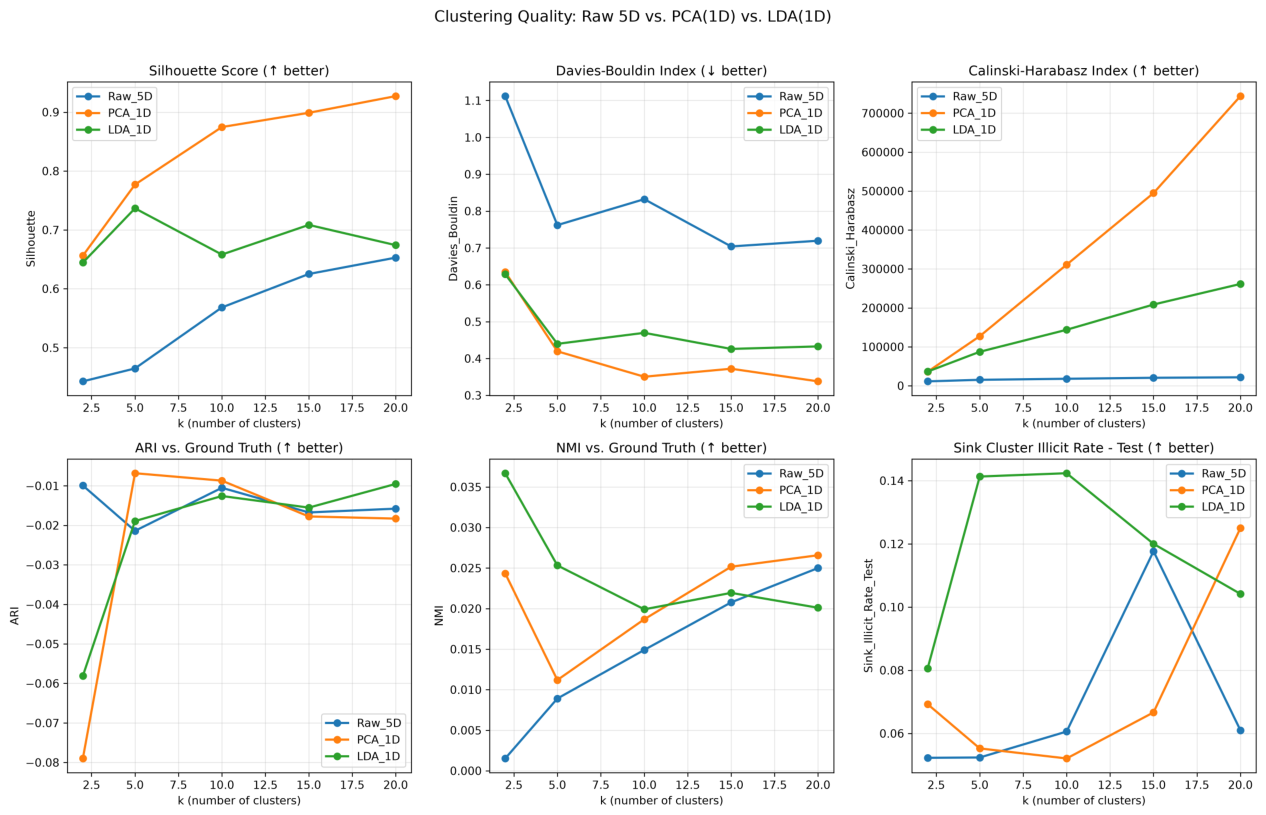
Figure 5.
Cluster-to-ground-truth confusion matrices on the test set for three projections. Left: Raw 5D (sink cluster C6, ARI=). Center: PCA(1D) (sink cluster C5, ARI=). Right: LDA(1D) (sink cluster C3, ARI=). Only LDA concentrates illicit nodes in a single high-purity sink cluster.
Figure 5.
Cluster-to-ground-truth confusion matrices on the test set for three projections. Left: Raw 5D (sink cluster C6, ARI=). Center: PCA(1D) (sink cluster C5, ARI=). Right: LDA(1D) (sink cluster C3, ARI=). Only LDA concentrates illicit nodes in a single high-purity sink cluster.
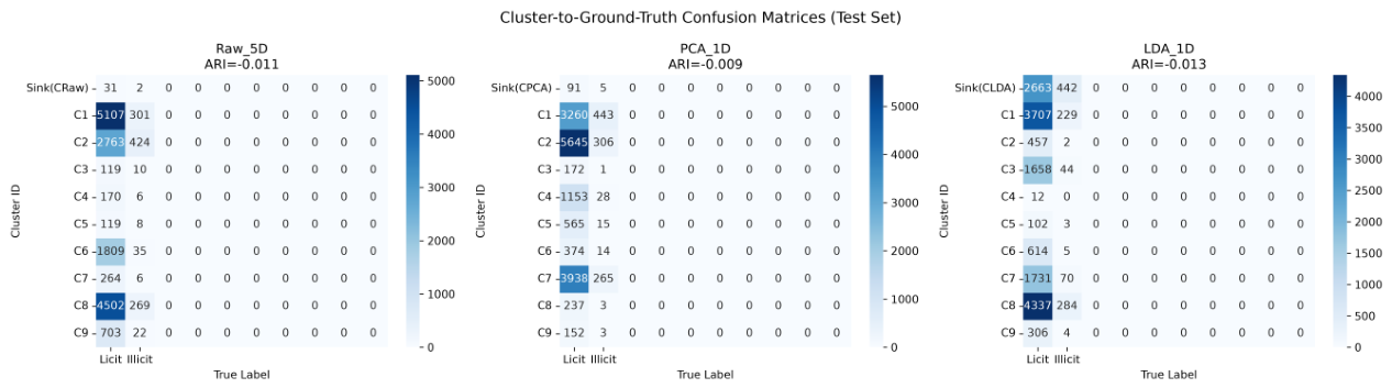
Figure 6.
Stability of the clusters over 20 independent trials using bootstrap clustering. Left graph: number of occurrences a node is assigned to the sink cluster. Right graph: Illicit rate of nodes assigned in x clusters. Where it has consistently been assigned to a sink cluster ( of the times), there illicit rates are percentage points higher than those not being exposed to the illicit clusters.
Figure 6.
Stability of the clusters over 20 independent trials using bootstrap clustering. Left graph: number of occurrences a node is assigned to the sink cluster. Right graph: Illicit rate of nodes assigned in x clusters. Where it has consistently been assigned to a sink cluster ( of the times), there illicit rates are percentage points higher than those not being exposed to the illicit clusters.
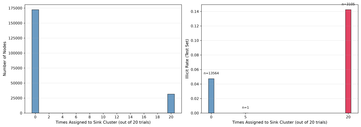
Figure 7.
Test-set convergence curves for all configurations over 100 epochs. It demonstrates test F1-Illicit gradually improves as training epoch increases in the proposed model 1 (LDA-log + clustering), which means that machine learning about the minority class is stable.
Figure 7.
Test-set convergence curves for all configurations over 100 epochs. It demonstrates test F1-Illicit gradually improves as training epoch increases in the proposed model 1 (LDA-log + clustering), which means that machine learning about the minority class is stable.
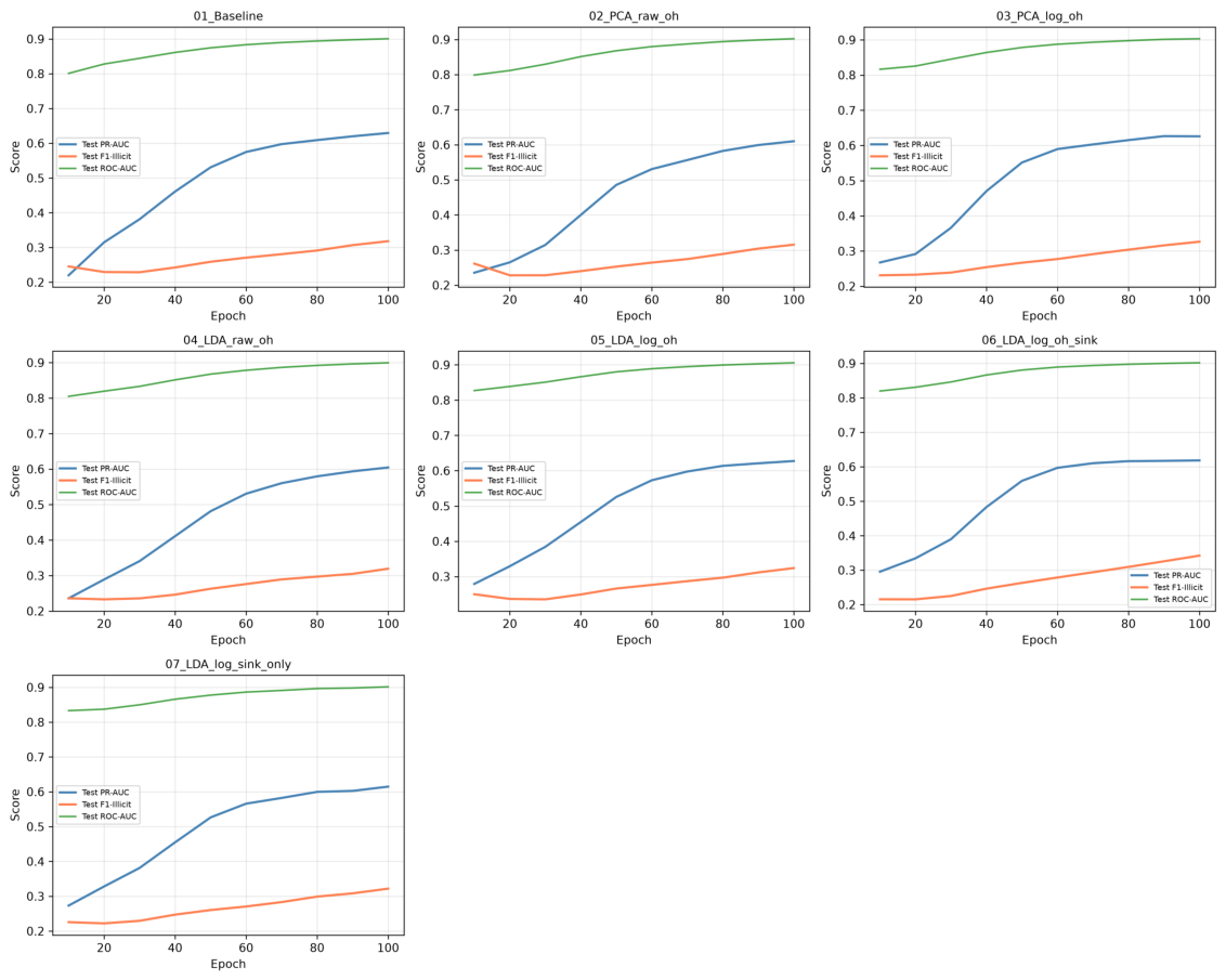
Table 1.
Clustering quality comparison for k-Means algorithm() on raw 5D features, PCA(1D) of structural features and LDA(1D) structural features. Indexes are computed within the training set given the training set labels. The larger the silhouette and NMI values are, the better the clusters are clustered. The smaller DB index is, the better the cluster. The sink illicit rate is calculated by applying and comparing results to the held out test set.
Table 1.
Clustering quality comparison for k-Means algorithm() on raw 5D features, PCA(1D) of structural features and LDA(1D) structural features. Indexes are computed within the training set given the training set labels. The larger the silhouette and NMI values are, the better the clusters are clustered. The smaller DB index is, the better the cluster. The sink illicit rate is calculated by applying and comparing results to the held out test set.
| Projection | Silhouette | Davies-Bouldin | Calinski-Harabasz | NMI | Sink Illicit Rate (Test) |
|---|---|---|---|---|---|
| Raw 5D (standardized) | 0.568 | 0.832 | 17,938 | 0.015 | 6.06% |
| PCA(1D) + log | 0.875 | 0.351 | 310,950 | 0.019 | 5.21% |
| LDA(1D) + log | 0.658 | 0.470 | 143,746 | 0.020 | 14.24% |
Table 2.
External clustering evaluation: K-Means () on raw 5D features, PCA(1D), and LDA(1D) of log-structural features. Metrics computed on the training set with known labels. Higher NMI indicates better alignment with ground truth. The Sink Illicit Rate is computed on the held-out test set.
Table 2.
External clustering evaluation: K-Means () on raw 5D features, PCA(1D), and LDA(1D) of log-structural features. Metrics computed on the training set with known labels. Higher NMI indicates better alignment with ground truth. The Sink Illicit Rate is computed on the held-out test set.
| Projection | ARI | NMI | FMI | Sink Illicit Rate (Test) |
|---|---|---|---|---|
| Raw 5D (standardized) | ||||
| PCA(1D) + log | ||||
| LDA(1D) + log |
Table 3.
Clustering-to-classification evaluation: GraphSAGE performance about features generated from clustering. All metrics were calculated on test set (time steps 35–49) of Elliptic. Bold are best values per column.
Table 3.
Clustering-to-classification evaluation: GraphSAGE performance about features generated from clustering. All metrics were calculated on test set (time steps 35–49) of Elliptic. Bold are best values per column.
| Configuration | PR-AUC | F1-Macro | F1-Illicit | Recall@1% | ROC-AUC |
|---|---|---|---|---|---|
| A: Baseline (no clustering) | 0.6295 | 0.5894 | 0.3182 | 0.1413 | 0.9006 |
| B: Raw 5D + clustering | 0.5922 | 0.5736 | 0.3004 | 0.1376 | 0.8949 |
| C: PCA(log) + clustering | 0.6216 | 0.5967 | 0.3244 | 0.1431 | 0.9006 |
| D: LDA(log) + clustering (Proposed) | 0.6278 | 0.6152 | 0.3454 | 0.1459 | 0.9014 |
Table 5.
Full Ablation: Seven Feature Configurations on Elliptic Test-Set, best values highlighted in bold.
Table 5.
Full Ablation: Seven Feature Configurations on Elliptic Test-Set, best values highlighted in bold.
| Model | Dim | PR-AUC | F1-Macro | F1-Illicit | Recall@1% | ROC-AUC |
|---|---|---|---|---|---|---|
| Baseline | 165 | 0.6295 | 0.5894 | 0.3182 | 0.1413 | 0.9006 |
| PCA(raw) + one-hot | 175 | 0.6101 | 0.5885 | 0.3155 | 0.1422 | 0.9021 |
| PCA(log) + one-hot | 175 | 0.6266 | 0.5879 | 0.3162 | 0.1413 | 0.9015 |
| LDA(raw) + one-hot | 175 | 0.6046 | 0.5914 | 0.3194 | 0.1422 | 0.8994 |
| LDA(log) + one-hot | 175 | 0.6274 | 0.5939 | 0.3240 | 0.1431 | 0.9058 |
| LDA(log) + one-hot + sink | 176 | 0.6184 | 0.6121 | 0.3423 | 0.1450 | 0.9017 |
| LDA(log) + sink only | 166 | 0.6147 | 0.5922 | 0.3218 | 0.1422 | 0.9013 |
Disclaimer/Publisher’s Note: The statements, opinions and data contained in all publications are solely those of the individual author(s) and contributor(s) and not of MDPI and/or the editor(s). MDPI and/or the editor(s) disclaim responsibility for any injury to people or property resulting from any ideas, methods, instructions or products referred to in the content. |
© 2026 by the authors. Licensee MDPI, Basel, Switzerland. This article is an open access article distributed under the terms and conditions of the Creative Commons Attribution (CC BY) license (http://creativecommons.org/licenses/by/4.0/).
Copyright: This open access article is published under a Creative Commons CC BY 4.0 license, which permit the free download, distribution, and reuse, provided that the author and preprint are cited in any reuse.