

Submitted:
01 September 2026
Posted:
01 September 2026
You are already at the latest version
Abstract
Typical machine learning forecasting approaches, optimized via mean squared error, struggle in decision settings requiring directional consistency. The Maximum Agreement Linear Predictor (MALP) framework addresses this by maximizing Lin’s Concordance Correlation Coefficient (CCC), but its meta-learner value under real, weak-signal conditions is untested. We evaluate a two-stage MALP-Meta architecture (four base models, a CCC-optimized meta-learner) on real hourly S&P 500 (SPY) data (n = 5032; 2023–2026), with every result cross-validated across two computing environments. Only Ridge achieves significant directional accuracy (52.7%, p = 0.037); no MALP-Meta variant improves on this, and we diagnose a previously undocumented pathology in which CCC optimization collapses toward a constant under weak signal. Of three temporal robustness strategies, only stable feature selection matches Ridge’s significance (52.5%, p = 0.048). Under an externally-defined stress regime (VIX>25), one meta-learner configuration improves simultaneously on concordance and direction, an unconfirmed signal (p = 0.291). Sensitivity analysis shows the primary result is fragile to the evaluation split. These findings affirm rather than overturn the conventional agreement–error trade-off: agreement-based meta-learning’s real-world value is modest, conditional on genuine market stress, and detectable only through rigorous cross-validation and sensitivity analysis.
Keywords:
maximum agreement linear predictor
; concordance correlation coefficient
; directional forecasting
; equity markets
; machine learning
; ensemble meta-learning
; reproducibility
; sensitivity analysis
; time series analysis
1. Introduction
The dominant framework in statistical and machine learning forecasting, based on least-squares linear predictors and mean-squared error minimization, fundamentally misaligns with the operational goals of various real-world decision-making processes [1,2]. While metrics such as mean squared error (MSE) optimally estimate conditional means under quadratic loss functions, they remain largely insensitive to a forecast’s directional consistency: the critical ability to predict whether a quantity will increase or decrease relative to its current state. In areas such as trading, portfolio allocation, and macroeconomic policy making, the usefulness of a forecast is mostly based on this directional signal, not the exact size of the prediction error. A market participant operating in intraday equity markets, for instance, profits from correctly anticipating whether prices will rise or fall in the next hour, not from minimizing the mean absolute dollar error of price predictions.
This misalignment stems from the core mathematical properties of the least-squares linear predictor, derived from minimizing expected squared error. The optimization returns the conditional mean as the ideal predictor; however, this formulation does not ensure that the predictor will consistently reflect the direction of changes in the target variable. As a result, a model might achieve low mean squared error while exhibiting poor directional accuracy, which represents a major failure mode for decision-making under uncertainty.
Recent theoretical advances have introduced the Maximum Agreement Linear Predictor (MALP) framework [3,4], which fundamentally reframes the forecasting objective from proximity to agreement. MALP directly addresses the limitations of least-squares estimation by optimizing for Lin’s Concordance Correlation Coefficient [5], a metric that rigorously quantifies the agreement between two variables as their deviation from the 45-degree line of perfect concordance. Unlike Pearson correlation, which measures linear association around any fitted line, the CCC explicitly evaluates how closely observations align with the identity line where predicted values exactly equal realized values [6]. This distinction is critical for forecasting applications where we seek not merely correlated predictions but predictions that agree with outcomes in both magnitude and direction.
The gap this study addresses. Although MALP exhibits theoretical sophistication and has shown benefits in controlled environments [3,4], existing evaluations have concentrated on stationary settings with strong, well-behaved signal. Three gaps follow. First, whether MALP-style agreement optimization retains its advantages as a meta-learner combining base models with only weak, real-world signal, the typical condition in liquid, near-efficient markets, has not been empirically established. Second, the concept drift literature [7,8,9,10] has developed adaptation techniques almost exclusively for error-minimizing objectives; whether these transfer to an agreement-optimized objective, and under what conditions they help or harm, remains largely untested outside controlled or synthetic settings. Third, the numerical behavior of CCC-based gradient optimization under weak signal has not been characterized; whether it degrades gracefully or fails in specific, diagnosable ways is an open question with direct practical consequences.
Our contribution. This study addresses these gaps through a real-data empirical investigation designed to test, rather than assume, MALP-Meta’s practical value. First, we implement and evaluate the full architecture, four heterogeneous base models combined via a CCC-optimized meta-learner, on real, verifiable equity data, with every result independently reproduced across two computing environments (Section 8). Second, we evaluate three temporal robustness strategies under a two-layer design (a standard chronological holdout and a secondary, externally-defined stress regime), distinguishing findings that hold under ordinary conditions from those that emerge only under genuine stress. Third, where results diverge from what stationary-setting theory predicts, we diagnose the mechanism directly, identifying a specific numerical pathology in CCC-based gradient optimization under weak signal and evaluating two practical mitigations. Fourth, we treat ablation analysis, sensitivity analysis, and transparent disclosure of null or fragile results as first-class components of this study, on the view that a method’s real effect sizes, and the conditions under which they hold, are more useful to a practitioner than a single headline number.
Sections 2 and 3 review the literature and develop the theoretical framework. Section 4 and 5 present the methodology and results together, subsection by subsection, so each method sits beside its own finding rather than in a separate part of the paper. Section 6 through 8 discuss the implications, conclude, and document reproducibility.
2. Literature Review
2.1. Classical Forecasting and the Limits of Error-Based Optimization
Predictive modeling in statistics and econometrics rests on classical least-squares methods [11], extended to high-dimensional settings through Ridge [12] and Lasso [13] regularization. Modern machine learning methods (gradient boosting, random forests, deep networks) retain the same underlying objective, minimizing squared or absolute error, despite far greater model complexity. This is mathematically convenient, since squared-error loss is everywhere differentiable and underlies the conditional-mean optimality result that anchors modern estimation theory, but it introduces a well-documented pathology: models trained to minimize MSE hedge toward the unconditional mean, systematically under-predicting the extreme, directionally consequential events that matter most for decisions in volatile domains such as financial markets.
2.2. Concordance Correlation and Maximum Agreement Linear Predictors
Lin’s Concordance Correlation Coefficient [5,14] addresses this gap by measuring agreement with the 45-degree identity line rather than mere linear association, combining precision and accuracy into a single index with an established biostatistics literature on its estimation and properties [6,15,16,17]. Wadoux Minasny [18] caution that CCC alone can be uninformative about the separate contributions of correlation, bias, and scale, motivating its use alongside complementary metrics rather than in isolation: the multi-metric approach we adopt in Section 5.2. Building on this foundation, Kim et al. [3], Kim et al. [4] formalized the Maximum Agreement Linear Predictor (MALP), proving that it targets a fundamentally different estimand than the least-squares predictor and yields systematically higher concordance at the cost of modestly higher error in stationary settings. Early extensions [19,20] have applied MALP-style agreement optimization to financial and economic forecasting, but exclusively under conditions of mild or absent non-stationarity.
2.3. Temporal Distribution Shift and Concept Drift
A parallel literature addresses the fact that the data-generating process underlying a time series rarely stays constant. Gama et al. [7] taxonomize drift into gradual, sudden, and recurring forms, while Zhang et al. [8] distinguish temporal shift (marginal feature distributions changing) from concept drift (the conditional relationship itself changing). Mitigation strategies include adaptive reweighting [9], input/output normalization [10], instance-wise normalization [21], and online ensembling [22,23]. Every one of these methods, however, targets error minimization as its implicit success criterion; none examines whether agreement-based objectives exhibit different robustness properties under shift.
2.4. Directional Forecasting and Market Efficiency in Equity Markets
The empirical domain of this study, directional forecasting of hourly equity returns, sits within a long-standing literature on market efficiency and predictability. The Efficient Market Hypothesis [24] holds, in its semi-strong form, that security prices rapidly incorporate publicly available information, implying that historical price and volume data alone should carry limited power to predict future returns; this is the theoretical backdrop against which any directional forecasting claim in liquid equity markets must be read; a genuine, reproducible directional edge in such a setting is expected to be small, not large, and any large or dramatic reported effect on real market data warrants particular scrutiny. Gu et al. [25] demonstrate that machine learning methods can nonetheless extract modest, economically meaningful signal from equity return prediction at scale, establishing the general viability of the model families this study also employs (regularized linear models, tree ensembles) while documenting that realized out-of-sample predictability is consistently far smaller than headline in-sample or synthetic-data results would suggest. Krauss et al. [26], evaluating gradient-boosted trees, deep networks, and random forests specifically on S&P 500 constituents (the same underlying index family studied here) similarly report that statistically detectable predictability exists but is modest and requires careful out-of-sample validation to distinguish from overfitting. This literature motivates both this study’s empirical expectations (real effects should be small) and its methodological emphasis on independent cross-validation, ablation, and sensitivity analysis (Section 5.4, 5.8) as safeguards against mistaking noise or a fragile analytical choice for genuine predictability.
Summary of the Related-Work Landscape
Table 1 summarizes these five streams, highlighting where each converges with the present study and the specific gap it leaves open.
As the table makes clear, no existing study sits at the intersection of agreement-based optimization and temporal robustness. Section 2.5 positions our contribution precisely at that intersection.
2.5. Positioning the Current Work
This study sits at the intersection of two literatures that have not previously been combined: MALP’s theoretical foundations, established in stationary settings (Section 1), and the concept drift literature’s adaptation techniques, developed exclusively for error-minimizing objectives. We evaluate temporal robustness strategies designed specifically for MALP-based forecasting in a real, liquid equity market application, under the ordinary, and in one respect (Section 5.6) genuinely stressed, non-stationarity that characterizes real financial markets.
3. Theoretical Framework
Our MALP-Meta framework integrates three theoretical traditions to generate testable empirical propositions regarding the behavior of agreement-based forecasting under temporal distribution shifts. This section develops the theoretical foundation systematically, progressing from statistical learning theory through concordance correlation properties to decision-theoretic considerations, culminating in four propositions that we evaluate empirically in Section 5, each stated with intuition and a formal proof.
3.1. Statistical Learning Theory: Reframing Empirical Risk Minimization
Classical statistical learning theory frames predictive modeling as empirical risk minimization over a hypothesis space [27]. Given training data consisting of feature vectors and target values , we seek a predictor function that minimizes expected loss over the true but unknown data-generating distribution. For a specified loss function , the population risk is
and the empirical risk minimization principle selects the predictor minimizing the sample analogue
The prevailing paradigm uses squared error loss , yielding
Under suitable regularity conditions, the solution is the conditional mean function . For linear predictors , empirical risk minimization reduces to ordinary least squares,
with closed-form solution , provided is invertible.
We propose an alternative risk formulation that shifts the learning objective from proximity to agreement, following Kim et al. [3], Kim et al. [4]. Define the agreement loss
where is Lin’s Concordance Correlation Coefficient computed over the joint distribution of realizations and predictions. The population risk under agreement loss is
and the Maximum Agreement Linear Predictor solves
Maximizing concordance correlation is equivalent to minimizing agreement loss. This reformulation substantially affects the resulting predictor: whereas the least-squares predictor targets the center of the conditional distribution regardless of its relationship to realized values, MALP explicitly seeks predictions that agree with realizations by maximizing alignment along the identity line.
This distinction is most evident in directional forecasting. Define the directional agreement indicator
which indicates whether a prediction correctly identifies the direction of change, stated here in the general, level-based notation common to the wider MALP literature, where denotes a raw target series (e.g. a price level) and directional accuracy concerns the sign of period-over-period change. Population directional accuracy is
Section 4.1 defines this study’s specific target variable as itself already a return rather than a price level, which simplifies this general definition to direct sign agreement; Section 5.2 states the resulting operational formula used throughout this study’s results. The decomposition links concordance correlation to directional correctness, where captures bias and scale agreement. A strong linear relationship, combined with comparable patterns of growth and decline between forecasts and realizations, is necessary for high concordance correlation. The relationship is not deterministic (pathological examples with high CCC but low directional accuracy, or vice versa, can be constructed), but maximizing CCC generally improves directional accuracy by enforcing alignment along the concordance line, particularly when data exhibit genuine trends rather than random fluctuation around a constant mean.
Proposition 1
(Directional Superiority in Agreement Optimization). Under temporal stationarity and bounded fourth moments, a predictor that maximizes concordance correlation satisfies , with strict inequality when the conditional distribution of Y given X exhibits temporal persistence in directional movements.
Intuition. Agreement-based optimization targets alignment along the 45-degree concordance line, implicitly rewarding directional consistency, whereas MSE minimization targets magnitude accuracy without regard for direction. When outcomes exhibit momentum (positive autocorrelation), directional signals become more predictable, amplifying this advantage. The inequality, rather than a fixed gap, reflects that the improvement’s magnitude depends on signal-to-noise ratio and the strength of temporal persistence.
Proof. Let denote the stationary joint distribution of , and define and . Directional accuracy is . Recall ; maximizing requires high covariance, low bias, and matched variance, and the covariance term rewards alignment of Y and around their respective means, which is directly related to directional agreement. Under temporal persistence (), directional movements exhibit momentum, and a concordance-maximizing predictor must align with this momentum to achieve high covariance, whereas focuses solely on minimizing squared deviations without explicit directional consideration. By the ergodic theorem, . Since explicitly maximizes alignment of and , it achieves higher directional alignment than whenever , with strict inequality except in degenerate cases where the two objectives coincide. ▪
3.2. Concordance Correlation Theory: Mathematical Properties and Optimization
The concordance correlation coefficient possesses mathematical properties that make it particularly suitable as a learning objective for directional forecasting [5,6,14]. In terms of sample moments,
where is the sample covariance, and are sample variances, and are sample means. The CCC attains its theoretical maximum of unity if and only if , , and hold simultaneously, and its minimum of negative unity under perfect negative correlation with no bias or scale mismatch.
A critical property for optimization is that CCC is differentiable almost everywhere with respect to predictions, enabling gradient-based optimization. The chain rule can be applied to compute , though the nonlinear dependence on means, variances, and covariances makes the resulting expressions complex; modern automatic differentiation frameworks such as PyTorch handle this computation efficiently, making CCC maximization tractable even for large datasets and high-dimensional feature spaces.
The optimization landscape of CCC maximization differs from that of MSE minimization. While MSE is convex for linear models, yielding a unique global minimum, CCC is generally non-convex with the potential for multiple local maxima, requiring careful initialization; in practice, initializing from the least-squares solution, which already achieves some baseline agreement, typically leads to satisfactory outcomes. The sensitivity of CCC to bias and scale differences implies that maximizing CCC implicitly encourages predictions to match not only the correlation structure but also the central tendency and dispersion of the target. Systematic bias, such as persistent over- or under-prediction, degrades CCC by increasing the bias-correction term , and such bias tends to produce directional errors: systematically high predictions fail to capture downward movements, while systematically low predictions overlook upward movements. By penalizing bias, CCC maximization encourages predictions that more closely track realized values in both level and direction.
Proposition 2
(Concordance Consistency). The Maximum Agreement Linear Predictor estimator satisfies when evaluated on the training distribution, with the inequality potentially reversed under distribution shift if the MALP solution captures patterns specific to the training period.
Intuition. MALP directly optimizes CCC and so necessarily achieves higher expected training-period concordance than OLS. This does not guarantee superior test-period performance under non-stationarity: if MALP exploits training-specific patterns, it may generalize poorly once those patterns change, motivating the temporal robustness strategies of Section 4.
Proof. By construction, on the training sample, so on that sample, with equality only in degenerate cases where the MSE and CCC objectives coincide; taking expectations over the training distribution establishes the training-period inequality. Under , the test-period CCC depends on , , and bias terms evaluated under the new distribution. If exploits training-specific covariance structure that does not persist under , while is comparatively more robust to certain classes of shift, the ranking can reverse: , depending on shift type and magnitude. ▪
3.3. Bayesian Decision Theory and Asymmetric Loss Functions
Forecasts serve as inputs to decision-making processes, and their usefulness depends on the loss function governing decisions [1,2] rather than any intrinsic property of predictive accuracy. Let denote an action from a feasible action space, Y the uncertain future state, and the loss incurred when action a is taken and state Y is realized. Given a forecast distribution , the optimal action minimizes expected loss:
In many trading and portfolio-allocation applications, the decision-relevant loss function is asymmetric. Consider a market participant deciding whether to hold a long position based on a directional price forecast: if the forecast indicates an upward move but the price falls, the participant incurs a realized loss on an open position; if the forecast indicates a downward move and the position is closed but the price then rises, the participant forgoes the unrealized gain. The magnitude of these losses typically differs depending on position sizing, holding costs, and risk limits. We formalize this asymmetry as
where represent the costs per unit of under- and over-prediction, respectively. In risk-managed trading settings, taking on directional exposure that turns out wrong typically incurs a materially different cost than under-committing to a correct directional view, since the latter can often be corrected through incremental position-sizing while the former exposes capital directly to the loss.
Directional errors (predicting an increase when a decrease occurs, or vice versa) tend to produce larger decision losses than magnitude errors of equivalent size that preserve correct directionality. A forecast that correctly predicts an upward movement but underestimates its magnitude allows appropriate positioning, incurring only the cost of suboptimal quantities; a forecast that predicts the wrong direction entirely leads to complete mis-positioning and the full opportunity cost of forgone action. Under asymmetric loss, the optimal point forecast is a weighted quantile of the conditional distribution rather than the conditional mean, but in operational settings decision-makers often apply simple threshold rules to point forecasts, making forecasts that consistently predict the correct direction, even with imperfect magnitude, more valuable than forecasts with lower magnitude error but poorer directional consistency.
Proposition 3
(Decision Regret Under Agreement Optimization). Under asymmetric loss functions with directional sensitivity, the expected decision regret
is lower for decisions based on MALP forecasts than for those based on LSLP forecasts, when the cost of directional errors exceeds the cost of magnitude errors conditional on correct directionality.
Intuition. Many decisions carry asymmetric costs where directional errors are disproportionately costly relative to magnitude errors within the correct direction. Incorrect price-direction forecasts lead to costly hedging errors, whereas modest magnitude errors with correct direction can be managed through incremental rebalancing. MALP’s focus on concordance aligns with such loss structures, reducing expected decision regret even when error metrics are marginally higher.
Proof. Consider the asymmetric loss if directionally correct and if directionally incorrect, with . The optimal decision rule depends primarily on when , since directional errors dominate the loss, so regret is approximately . By Proposition 1, MALP achieves higher directional accuracy than LSLP under temporal persistence, so whenever , with the gap increasing in the ratio . ▪
3.4. Temporal Distribution Shifts: Implications for Agreement-Based Learning
The theoretical advantages of MALP established above rely on implicit stationarity assumptions. When the joint distribution of features and target variables changes over time (an assumption violated in virtually all real-world forecasting applications [7,8]), the properties of both LSLP and MALP estimators require reconsideration. Let denote the joint distribution of at time t; distribution shift occurs when for .
Following Zhang et al. [8], we distinguish temporal shift, where the marginal distribution changes while remains stable, from concept drift, where the conditional distribution itself evolves. Both frequently co-occur, complicating adaptation [9,10]. For feature j, let and denote training- and testing-period means. The magnitude of temporal shift is quantified as
where is a small constant preventing division by zero.
The effect of distribution shift on MALP performance depends on its nature. Performance deteriorates for both LSLP and MALP when features that were predictive during training lose predictive power due to altered associations. Adaptive normalization can mitigate shifts in magnitude while preserving conditional relationships; however, if the agreement structure itself changes (for example, a feature positively associated with the target during training becomes negatively associated during testing), optimizing MALP on training data may actively harm test performance by exploiting relationships that no longer hold.
These considerations motivate three strategies for enhancing temporal robustness in MALP-Meta: (i) rolling window validation, which keeps training and testing periods close in time, reducing exposure to large shifts at the cost of smaller training samples; (ii) domain-adaptive learning, which uses adversarial training to explicitly align feature distributions across time; and (iii) temporally stable feature selection, which prioritizes features exhibiting minimal distributional variation, trading some information content for greater reliability.
Proposition 4
(Temporal Stability Dominance). When feature magnitude changes
exceed 100% for a substantial fraction of features, model performance is primarily determined by feature temporal stability rather than training-period feature importance. Predictors using stability-based feature selection achieve superior out-of-sample concordance correlation relative to those using importance-based selection:
Intuition. When distributions shift substantially, features important during training may lose predictive value if their relationship with the target changes. Temporally stable features maintain consistent relationships across periods, improving generalization even if less important during training. This is a trade-off between exploiting training-period patterns (importance) and robustness to change (stability); beyond a critical threshold, empirically around 50–100% average shift magnitude, stability supersedes importance as the primary determinant of forecast quality.
Proof. Let denote features selected by training-period importance and denote features selected by temporal stability, with predictors and trained on each set respectively. Decompose test error as irreducible error plus model error: . For , features in exhibit by assumption, so substantially, and evaluates the training-period conditional expectation in regions of the feature space rarely observed during training, inducing large model error. For , features in satisfy by construction, and under the assumption that conditional relationships are preserved for stable features, , yielding small model error. Since CCC penalizes both weak correlation and systematic bias, and suffers on both dimensions while does not, . ▪
4. Methodology
We note at the outset that the theoretical propositions developed in Section 3 are not uniformly confirmed by the empirical work below. Proposition 3 (decision regret under asymmetric loss) is not empirically tested in this study at all; we did not construct an asymmetric-loss decision simulation, and its inclusion in Section 3 should be read as a theoretical extension motivating future work rather than a claim we go on to validate. Proposition 4 (temporal stability dominance) is stated to hold specifically when feature-magnitude shifts exceed roughly 100% for a substantial fraction of features; as detailed in Section 5.1, the real shift magnitudes observed in this study’s data never approach that threshold, so Proposition 4’s own stated precondition is not met here, and the corresponding empirical result (Section 5.5) should be read as a related but distinct, much milder finding rather than a direct confirmation. Propositions 1 and 2 receive partial empirical contact, discussed against the real results in Section 5.3 and 6.1; Proposition 1 specifically is not supported by our findings, since the MALP-Meta meta-learner does not achieve higher directional accuracy than the strongest individual baseline in this study. We report this transparently here, before presenting the methodology, because a methodology section that implies full theoretical validation without disclosing this would misrepresent what the empirical work below actually establishes.
4.1. Data Description
Our empirical analysis uses hourly OHLCV (open, high, low, close, volume) data for SPY, the SPDR S&P 500 ETF Trust, obtained via the Yahoo Finance data interface, spanning September 15, 2023 through August 13, 2026 (regular U.S. equity trading hours, seven hourly bars per session). After removing rows with missing values (three isolated zero-volume bars, plausibly low-liquidity edge prints, out of 5082 total) and the warmup period required by rolling-window feature construction, the dataset comprises hourly observations. The target variable is the next-bar log return, , where is the closing price of hourly bar t.
The target exhibits pronounced excess kurtosis (24.1) and near-zero skewness (); a Shapiro–Wilk test decisively rejects normality (, on a representative 5000-observation subsample), consistent with the well-documented fat-tailed behavior of real financial returns. Lag-1 autocorrelation of hourly returns is , and a Ljung–Box test at 10 lags is technically significant () but with individual autocorrelation coefficients uniformly below in magnitude: a statistically detectable but economically negligible departure from independence, consistent with near-efficient hourly equity microstructure rather than any strong exploitable autoregressive structure. Directional balance across the full sample is 53.4% up-moves to 46.4% down-moves, reflecting the bull-market character of the sample period rather than a designed 50/50 split.
We engineer 36 predictive features directly from the raw OHLCV series, organized into six families: lagged and cumulative returns (six lag lengths, five momentum windows), rolling realized volatility (four window lengths), momentum oscillators (RSI at two lookback periods), range-based volatility measures (true range, Average True Range at three window lengths, high–low and open–close range percentages), volume-derived features (volume z-score, a short/long volume ratio, log-volume), moving-average deviations and MACD-family trend indicators, and calendar features (hour of day, day of week, month-end indicator). All features are constructed using only information available at or before the time of prediction, using standard rolling-window operations with no forward-looking computation. This engineered set deliberately favors stationary constructs (returns, ratios, and rolling statistics) over raw price levels, a design choice that materially affects the magnitude of temporal distribution shift observed in Section 5.1.
4.2. Data Diagnostics and Preprocessing
Prior to model training, we conduct a standard pre-modeling diagnostic battery: missingness screening (none present post-warmup), the normality assessment above, an Augmented Dickey–Fuller stationarity test on the target and a representative subset of engineered features (all reject the unit-root null at the 5% level, confirming the stationary-by-construction design intent), a Ljung–Box autocorrelation test, correlation-matrix and Variance Inflation Factor (VIF) screening for multicollinearity, and IQR-based and z-score-based outlier screening.
The VIF screening identifies severe multicollinearity among several engineered feature families (short-window momentum and moving-average-deviation constructs in particular, given their near-linear-dependence at short windows), with several features exhibiting VIF in excess of prior to any correction. We apply iterative VIF elimination (removing the single highest-VIF feature and recomputing until all remaining features satisfy , a conventional threshold), yielding a pruned set of 25 features from the original 36. An ablation analysis (Section 5.4, Arm B) subsequently establishes that this pruning, while numerically necessary for linear-model estimation, measurably degrades the performance of the tree-based base models, since multicollinearity is specifically a linear-model pathology to which decision-tree splitting is largely insensitive. We therefore adopt a per-model feature-set policy for the main results (Section 5.2): the pruned 25-feature set for OLS and Ridge, and the full 36-feature set for Random Forest and XGBoost.
Feature scaling uses robust normalization based on the median and interquartile range (IQR),
computed using training-period statistics only and applied identically to training and testing data, preventing test-period information from influencing preprocessing. We depart from a naive IQR denominator in one respect: for near-constant or binary features (for example, the month-end calendar indicator, where fewer than 25% of observations are non-zero, placing both the 25th and 75th percentiles at the same value and producing an IQR of exactly zero), we substitute the feature’s standard deviation as the scale denominator rather than an arbitrary small constant. An earlier implementation used a fixed floor in this degenerate case, which we found during development to inflate a single binary feature’s scaled values by a factor of approximately , corrupting the entire feature matrix for any unregularized downstream model; this was caught via an unregularized diagnostic model that failed catastrophically during development, and is corrected throughout this study’s pipeline. We record this correction explicitly because Ridge regression’s regularization and the tree-based models’ scale-invariance had largely masked the error’s effect on this study’s other reported results, and because transparent disclosure of caught-and-fixed implementation errors is, in our view, part of honest methodological reporting rather than a detail to omit.
4.3. Train–Test Splitting and Temporal Validation Protocol
We adopt a two-layer chronological evaluation protocol rather than a single fixed split, combining a primary standard temporal holdout with a secondary, externally-defined regime-conditional stress test, following recent practice in financial machine learning that treats regime-aware evaluation as a complement to, rather than a replacement for, conventional out-of-sample testing [28].
Primary split. The first 77.4% of chronologically ordered observations (; September 26, 2023 through December 17, 2025) form the training set, and the remaining 22.6% (; December 17, 2025 through August 13, 2026) form the test set. This proportional allocation was fixed prior to any outcome inspection, matching the proportional split used in prior work in this framework, and is not tuned to any result reported in Section 5; Section 5.8 reports a dedicated sensitivity analysis to this specific choice.
Secondary split. We additionally partition the sample using an externally validated, feature-independent stress indicator: the CBOE Volatility Index (VIX, FRED series VIXCLS). An hourly bar is assigned to the stress regime if its calendar date coincides with a day on which VIX closed above 25, a conventional threshold for elevated market stress given a long-run VIX average near 19–20 over the sample period. This threshold identifies 38 stress days clustering into three distinct real episodes within the sample window, pooled into a single stress-regime test set (); all remaining hours form the calm-regime training set (). Because this regime label depends only on VIX’s own publicly available closing values and is computed entirely independently of the 36 engineered predictive features, its use as an evaluation boundary carries no risk of being chosen to favor a particular empirical result.
4.4. Statistical Significance Testing
For directional accuracy, we test whether performance exceeds the 50% level expected under random guessing using a one-sided binomial test: under the null hypothesis, the number of correct directional predictions (excluding the small number of exact-zero-return bars, for which direction is undefined), and we compute . This test is applied uniformly to every directional-accuracy result reported in this study (Section 5.2–5.8) and is the sole formal significance test we employ.
We report CCC, RMSE, , and Kendall’s throughout as point estimates without an accompanying formal significance test in this study. Bootstrap resampling ( replications) for CCC comparisons and a Diebold–Mariano test [29] for error-metric comparisons were specified as part of this study’s original design but were not in fact implemented in the analysis pipeline that produced the results in Section 5; rather than retroactively describe tests that were not run, we correct the record here. We regard the resulting gap (point-estimate differences reported without a corresponding formal test of their statistical significance) as a genuine limitation of this study, discussed further in Section 6.6, and a natural target for a bootstrap-based CCC comparison in future revisions of this work.
4.5. Model Interpretability: Agreement-Based Feature Attribution
The nonlinear base learners within MALP-Meta, Random Forest and XGBoost in particular, are not directly interpretable at the individual-prediction level, motivating a feature attribution methodology to complement the meta-learner weight interpretation developed in Section 5.3. We deliberately depart from the two dominant post-hoc explanation frameworks, SHAP [30] and LIME [31], for reasons specific to this study’s setting rather than as a general critique of either method.
SHAP’s coalition-sampling estimators (KernelSHAP) and its tree-specific variant (TreeSHAP) rely on an assumption of feature independence when constructing counterfactual coalitions; Section 5.1 documents extreme multicollinearity and a systematic reversal in feature correlation structure between training and testing periods, precisely the condition under which Shapley-value attributions become unreliable [32]. LIME constructs local surrogate models by perturbing a neighborhood around each prediction and assumes that this local neighborhood is representative of the region in which the true function behaves approximately linearly; under the extreme temporal distribution shift that is the central subject of this paper, a neighborhood defined by training-period local structure is, by construction, not representative of test-period behavior, undermining the local-fidelity guarantee that motivates LIME’s design.
We instead propose Agreement-Based Permutation Importance (API), a model-agnostic attribution method that measures each feature’s contribution directly in the metrics this study is built around, concordance correlation and directional accuracy, rather than in the generic value-function terms SHAP and LIME were designed to explain. For a trained MALP-Meta pipeline and each feature j in the selected feature set , we permute the values of across the testing observations (breaking its association with the target while exactly preserving its marginal distribution) and recompute predictions using the already-trained base models and meta-learner weights, without retraining. The attribution scores are the resulting degradation in performance:
where and denote performance with all selected features intact and , denote performance with feature j permuted. We repeat this procedure over independent permutations per feature and report the mean attribution with a percentile-based confidence interval, following the general permutation-importance framework of Fisher et al. [33].
Naive permutation importance shares SHAP’s vulnerability to correlated features: permuting one feature in isolation while leaving correlated features untouched can produce unrealistic feature combinations and inflate or deflate apparent importance. We address this by additionally computing grouped permutation importance, in which features are first clustered by pairwise correlation (threshold ) and permuted jointly within each cluster rather than independently, following Strobl et al. [34]. This yields an importance score for each correlated group as a whole, avoiding the double-counting or masking that afflicts naive permutation under multicollinearity, and is directly relevant here given the correlation structure documented in Section 5.1.
To visualize how each feature’s marginal relationship with model output varies across its value range, we use Accumulated Local Effects (ALE) plots [35] rather than partial dependence plots. ALE estimates local effects using differences in predictions computed over conditional (rather than marginal) feature distributions, which prevents the extrapolation into unrealistic feature combinations that biases PDPs under correlated inputs: the same concern that motivates our departure from SHAP.
This methodology yields three complementary outputs, reported in Section 5.9: (i) individual API scores per selected feature, directly comparable in units of CCC and DA change; (ii) grouped importance scores for correlated feature clusters; and (iii) ALE curves for the highest-attribution features, showing the direction and shape of their marginal relationship with agreement-optimized predictions. Because API is computed post-hoc on frozen model parameters using only feature permutation, it adds negligible computational cost relative to the training pipeline described in Section 5.2–5.3, in contrast to SHAP’s coalition enumeration or LIME’s per-instance surrogate fitting, both of which scale poorly across the 25- or 36-feature sets used in this study, evaluated under three separate robustness strategies.
5. Results
5.1. Temporal Distribution Shift Characterization
We characterize temporal non-stationarity using two complementary, independently constructed evaluation layers rather than a single train–test split, following the two-layer design established in Section 4.3. The primary chronological split (77.4%/22.6%, , ) allocates the most recent portion of the two-year hourly SPY sample to testing. Under this split, the correlation between training- and testing-period feature means is , indicating that this window is characterized predominantly by mild, gradual non-stationarity rather than an abrupt distributional break: an honest empirical property of real, liquid, actively traded equity data, and consistent with efficient-market behavior over this period. Only a single engineered feature exceeds a 50% shift in mean magnitude under this split.
The secondary evaluation layer instead partitions the sample by an externally validated, feature-independent stress indicator: the CBOE Volatility Index (VIX, FRED series VIXCLS). Hourly bars falling on a calendar date where VIX closed above 25 (a conventional elevated-stress threshold, given a long-run VIX average near 19–20 over the sample period) are pooled into a stress-regime test set () spanning three distinct real episodes, most notably an April 2025 volatility spike (VIX peaking at 52.33) and a March–April 2026 episode; all remaining bars form the calm-regime training set (). Because the regime label is constructed entirely independently of the engineered predictive features, this partition carries no risk of being chosen to favor a particular result. Under this split, the correlation between calm- and stress-regime feature means falls to , with 18 of 36 features exhibiting shifts exceeding 50%, and realized volatility in the stress regime averaging 2.69 times its calm-regime level: a genuine, externally verified non-stationarity substantially exceeding what the primary chronological split exhibits. This two-layer design follows recent practice in financial machine learning of evaluating models separately under calm and externally-defined stressed regimes as a complement to, rather than a replacement for, conventional chronological out-of-sample testing [28].
5.2. Baseline Model Performance Under Standard Training
We implement four baseline models spanning classical statistical methods and modern machine learning, serving both as standalone forecasts and as the base layer for the MALP-Meta meta-learner (Section 5.3). OLS fits with on the pruned 25-feature set (Section 4.2). Ridge extends OLS with L2 regularization, , selected via 5-fold cross-validation over a logarithmic grid spanning to ; we standardize the target before cross-validation and invert on final predictions, since hourly returns’ very small natural scale () caused the cross-validation procedure to select degenerate boundary values of on the raw target in early implementations. Random Forest [36] aggregates 100 bootstrap-trained decision trees (square-root feature subsampling, minimum leaf size five) on the full 36-feature set. XGBoost [37] implements gradient-boosted trees (100 rounds, max depth three, learning rate 0.1, L2 leaf regularization) on the full 36-feature set.
We evaluate forecasting performance using six complementary metrics, reported together in Table 2 and throughout the results that follow, since each captures a distinct property of forecast quality that the others can miss. Root Mean Squared Error (RMSE), , and Mean Absolute Error (MAE), , capture magnitude accuracy, with RMSE weighting large errors more heavily and MAE more robust to outliers. The Coefficient of Determination, , captures explanatory power relative to the unconditional mean, ranging from 1 (perfect fit) down to , with negative values indicating performance worse than simply predicting the mean. The Concordance Correlation Coefficient,
this study’s central agreement metric (Section 3.2), combines correlation, scale agreement, and location shift into a single index, with higher values (closer to 1) indicating stronger agreement. Directional Accuracy is defined, following Section 3.1’s general level-based formulation , but simplifies in this study’s specific implementation because the target is itself already a return (Section 4.1) rather than a price level: with representing the most recently realized return rather than a price, the operative comparison reduces to direct sign agreement between the realized and predicted return,
which is the formula actually computed throughout this study’s results (a handful of exact-zero-return bars, for which sign is undefined, are excluded from n). We note this simplification explicitly because Section 3’s theoretical exposition is stated in the more general, level-based notation common to the wider MALP literature, and a reader comparing the two should not read the difference as an inconsistency. Kendall’s Tau, for , concordant and discordant pairs, is a non-parametric rank correlation reported alongside the other five as a robustness check against monotonic, non-linear association the other metrics might miss. In practice, as the results below illustrate directly, improvements on agreement or directional metrics can come at the cost of degradation on error metrics, rather than all six moving together.
Table 2 presents baseline model performance on the primary chronological test set. An ablation analysis (Section 5.4) established that the VIF-based multicollinearity pruning used to stabilize the linear models (Section 4.2) measurably degraded the tree-based models’ performance without a corresponding benefit, since multicollinearity is specifically a linear-model pathology that tree splits are largely immune to. We therefore report OLS and Ridge on the pruned 25-feature set (for which the pruning was designed) and Random Forest and XGBoost on the full 36-feature set; Section 5.4 reports the complete pruned-versus-full comparison for all four models.
Several patterns emerge. First, ranges from to : essentially none of the four baselines explains out-of-sample variance in next-hour returns beyond the unconditional mean, consistent with near-efficient hourly equity microstructure. Second, CCC values are uniformly small (0.0005 to 0.0265), reflecting weak agreement across all baselines under real market conditions. Third, and most notably, Ridge achieves directional accuracy of 52.69%, significant at the 5% level (): the only individual baseline to clear conventional significance. This is a modest but genuine, independently cross-validated effect (Section 4.4). Fourth, Random Forest and XGBoost, evaluated on the full feature set, achieve the highest CCC among baselines (0.0265 and 0.0176 respectively) without a corresponding directional-accuracy advantage, illustrating that agreement and directional correctness are related but distinct properties of a forecast (Section 3.2).
We emphasize a caveat developed further in Section 5.8: sensitivity analysis across nearby split points, run on this same pruned-25-feature Ridge specification, shows the significance is not robust to small changes in the train–test boundary: only 3 of 9 tested split points (0.700, 0.720, and the primary 0.774) reach . The primary split itself was fixed at 77.4% before any results were examined, matching the proportional allocation of prior work in this framework, so this is not a case of the split being tuned to produce significance; nonetheless, the result should be read as a real but fragile effect rather than a robust one.
Figure 1 shows cumulative actual and Ridge-predicted return across the primary test period, with a 48-hour rolling directional accuracy below it. Ridge’s predicted cumulative path is a near-straight, shallow line against the actual path’s real, noisy swings, an honest reflection of the model’s weak magnitude signal (Table 2’s near-zero ); the rolling DA panel shows the accuracy oscillating around, and at times meaningfully above, the 50% chance line and its binomial band, consistent with a real but modest, time-varying directional edge rather than a stable large one.
Figure 2 extends this comparison to Ridge’s in-sample (training-period) fit alongside its out-of-sample forecast. Real in-sample RMSE (0.0037) is, perhaps counterintuitively, slightly higher than real out-of-sample RMSE (0.0033), the reverse of the usual overfitting pattern where in-sample error is smaller. We attribute this to the heavy regularization Ridge’s cross-validation selects (Section 4.4): with pushed to a large value given the weak available signal, the model’s fitted line barely deviates from a constant drift in either period, so the RMSE ratio mostly reflects which period happened to have marginally larger realized return magnitude rather than a meaningful difference in model fit quality between the two periods. We deliberately annotate the figure with alongside RMSE (0.0014 in-sample, 0.0004 out-of-sample, both near zero) precisely because the fitted lines visually track the actual cumulative path closely, a byproduct of both the market period and the model’s near-constant output trending upward together, not of the model explaining real variation; without this explicit caveat, the visual alone could overstate the model’s actual skill.
5.3. MALP Meta-Learner Performance on Baseline Predictions
The core architecture implements MALP as a meta-learner combining the four base models’ predictions, following the two-stage stacking approach of Wolpert [38] but replacing the meta-learner’s error-minimizing objective with concordance maximization, per Kim et al. [3]. Level 0 generates out-of-fold base-model predictions on the training period via 5-fold time-series cross-validation (expanding-window folds respecting chronological order, avoiding the leakage of in-sample predictions), stacked into ; the first fold’s training portion lacks out-of-fold coverage, reducing the usable meta-learner training sample from to approximately 3245 observations. Level 1 is an affine combination , trained to minimize via automatic differentiation in PyTorch [39] with the Adam optimizer [40] (, , , , 200 epochs, gradient clipping at , learning-rate halving on a 50-epoch plateau).
We report three variants, motivated by a numerical pathology diagnosed during development. Because the four base models carry only weak signal (below), an unconstrained meta-learner is prone to a specific failure: as w shrinks during optimization, predictions collapse toward a near-constant value, at which point CCC’s numerator and denominator vanish together, so regardless of the constant’s value, and the loss surface goes locally flat with respect to , removing any gradient signal to correct an intercept that has drifted far outside the target’s natural scale during early updates, a pathology distinct from, though related to, the Ridge scale-mismatch of Section 5.2, and one we are not aware of being previously documented in the MALP literature. We therefore additionally report an L2 variant (an penalty on w) and a simplex variant (weights constrained to the probability simplex via softmax, the standard stacking convention [38]), alongside the vanilla unconstrained variant faithful to the architecture as originally specified. In all three, Z and Y are standardized prior to optimization for the same scale-matching reason as Ridge, with the learned affine map composed back into the original prediction scale for evaluation.
We assess the meta-learner applied to out-of-fold base-model predictions from the four baselines in Table 2.
Figure 3 and Figure 4 summarize performance across all four baselines and three MALP-Meta variants; exact values (RMSE, MAE, , CCC, DA, Kendall’s ) for each are as follows: Ridge (best baseline DA) 0.0033, 0.0021, 0.0004, 0.0005, 0.5269 *, ; XGBoost (best baseline CCC) 0.0033, 0.0021, , 0.0176, 0.5233, 0.0307; MALP-Meta vanilla 0.0047, 0.0034, , 0.0168, 0.4872, ; MALP-Meta L2 0.0040, 0.0028, , 0.0143, 0.4846, ; MALP-Meta simplex 0.0045, 0.0033, , 0.0281, 0.4916, (*; none of the three MALP-Meta variants achieves DA significantly different from chance, , , respectively).
The result is unambiguous and, we argue, more informative than a marginal improvement would have been: no MALP-Meta variant beats Ridge’s directional accuracy, and all three variants exhibit substantially worse than any individual baseline. The vanilla and simplex variants achieve higher nominal CCC than the best baseline CCC (0.0168 and 0.0281 vs. 0.0176); the L2 variant does not (0.0143). Where CCC does improve, this gain is purchased at a severe cost to error metrics and directional accuracy: the classic agreement–error trade-off reasserting itself under genuinely weak-signal conditions. Figure 4 adds a further layer: Ridge’s low CCC stems specifically from its bias-correction term (0.013, the lowest of the four), not from its correlation r (0.035, the highest of the four), while Random Forest and XGBoost show the opposite pattern, low r but comparatively healthy ; low CCC can arise from a poorly-correlated-but-well-calibrated model or a well-correlated-but-poorly-calibrated one, and these are not the same failure.
Diagnosing the vanilla variant’s optimization behavior is itself informative. When base-model weights shrink toward zero during training (which occurs naturally here, since none of the four base models carries strong, generalizable signal), the meta-learner’s predictions collapse toward a constant (the intercept). Because CCC’s numerator (covariance) and denominator (prediction variance) both vanish together when predictions are constant, CCC becomes identically regardless of the constant’s value: the loss surface goes flat with respect to the intercept, leaving no gradient signal to correct an intercept that has drifted away from the target’s true scale during early, noisy updates. This is a genuine numerical pathology of CCC-based optimization under weak signal, not an implementation error, and it motivates the L2 and simplex variants as practical safeguards beyond the gradient-clipping and denominator-stabilization already specified above.
A leave-one-base-model-out analysis (Section 5.4, Arm C) further shows that the simplex meta-learner’s nominal CCC advantage is driven almost entirely by a single base model, OLS: removing Ridge, Random Forest, or XGBoost individually changes CCC by less than 0.001 in either direction, while removing OLS produces a substantially larger drop. We report this OLS finding qualitatively rather than as a specific point estimate, since Section 8 documents that its exact magnitude was not stable across independent computing environments; the qualitative conclusion (the ensemble is not meaningfully diversified, and one base model is doing most of the work) held in both. Table 3 accordingly omits a “drop OLS” row.
5.4. Ablation Study
To isolate which components of the pipeline drive its performance, we conduct three ablation arms, all evaluated on the primary test set: Arm A compares the simplex meta-learner against a naive equal-weight average, isolating whether learning combination weights adds value; Arm B compares each baseline’s performance on the pruned 25-feature set against the full 36-feature set; Arm C retrains the simplex meta-learner four times, each excluding one base model, isolating its marginal contribution. Table 3 reports the results.
Arm A shows that the equal-weight average is, on balance, the more robust choice: it achieves a substantially better ( vs. ) and comparable directional accuracy to the learned simplex weights, despite the latter’s higher nominal CCC. Learning weights via CCC optimization is not a free upgrade over naive averaging in this setting, consistent with the classical bias–variance framing of ensemble methods [41]: a fixed, unlearned combination rule adds no estimation variance of its own, whereas a learned meta-learner’s additional degrees of freedom are only worth their variance cost when the base models carry enough real signal to reward the extra flexibility, which Section 5.3 shows is not the case here. Arm B shows that VIF pruning specifically harms the tree-based models: Random Forest’s CCC nearly ten-fold higher on the full feature set (0.0265 vs. 0.0028), and XGBoost’s roughly double (0.0176 vs. 0.0095), while the effect on OLS and Ridge is comparatively small. This is consistent with multicollinearity being a linear-model-specific pathology that decision-tree splitting is largely insensitive to, and directly motivates the per-model feature-set policy adopted in Table 2. Arm C confirms that OLS is the dominant contributor to the simplex ensemble’s CCC (Section 5.3); removing any of the other three base models changes CCC by at most 0.0005 in magnitude.
5.5. Temporal Robustness Strategy Comparison
We evaluate three temporal robustness strategies on the primary test period, using the full 36-feature set as their common starting point (Section 5.4, Arm B). Strategy 1 (Rolling Window) retrains a Ridge model on a sliding 168-hour window and forecasts the next 24 hours, stepping forward through the test period; we restrict retraining to Ridge alone given the cost of refitting four models at each of approximately 47 steps. Strategy 2 (Domain-Adaptive) augments a linear meta-learner operating on the scaled 36-dimensional feature representation with an adversarial domain-confusion mechanism: a discriminator is trained to distinguish training- from testing-period feature vectors while the meta-learner maximizes concordance correlation and simultaneously tries to fool the discriminator, via with (five discriminator updates per meta-learner update, 150 epochs). Strategy 3 (Temporally Stable Feature Selection) computes, for each feature j, a stability index and a Gini importance from a training-period Random Forest, combined as ; we select the top 15 features by this composite score (as in the original MALP framework, this idealized computation uses testing-period data unavailable in strict deployment, and Section 5.8 reports a sensitivity check on both k and the composite’s functional form) and retrain Ridge on the reduced set.
Table 4 compares the three strategies against a Ridge reference fit on the full 36-feature set (this reference differs from Table 2’s pruned-25-feature Ridge, per the Arm B rationale of Section 5.4; the two Ridge specifications are not interchangeable, and their p-values, 0.037 for the pruned specification and 0.048 here for the full specification, should not be read as the same result reported twice).
Temporally stable feature selection (Strategy 3) is the only strategy to improve on the full-feature reference: it achieves the highest of any strategy tested and the only positive among the three robustness strategies (0.0012; the full-feature reference is also positive at 0.0009) and matches the reference’s directional accuracy (0.5251, ) while using a feature set selected purely by a composite stability×importance score (Section 5.6) rather than the VIF-based criterion used elsewhere. Rolling window validation (Strategy 1) achieves the highest CCC among the three strategies (0.0127) but does not reach directional-accuracy significance (). Domain-adaptive MALP-Meta (Strategy 2) underperforms the reference on RMSE, , and directional accuracy (0.4819, , below chance), though its nominal CCC (0.0109) exceeds the reference (0.0013): the RMSE and degradation is consistent with known instability in adversarial domain adaptation when applied to weak-signal, low-dimensional representations [42]. An initial implementation of this strategy exhibited a further numerical instability, a scale mismatch between the Adam optimizer’s step size and the target’s small natural magnitude, resolved via the same target-standardization fix applied to the Ridge baseline (Section 5.2); Section 8 documents this as one of two implementation errors caught during development.
We caution against over-reading Strategy 3’s apparent parity with the reference as evidence of a large effect: both achieve identical directional accuracy on this specific split. Section 5.8’s split-point sweep was conducted on the Ridge reference model, not re-run for Strategy 3’s own feature-selection procedure at each split; we do not claim Strategy 3’s result has been separately tested for split-point sensitivity, only that its stated k and composite-weighting choices have (Section 5.8).
Figure 5 consolidates every model and strategy evaluated in Section 5.2–5.5 into a single visual summary across all six metrics. Color encodes relative standing within each metric column (amber indicates better performance, teal worse, with the direction of "better" inverted for RMSE before coloring so that amber consistently means the same thing in every column); the annotated number in each cell is always the real, un-transformed reported value. The visual pattern reinforces the numeric one: the three MALP-Meta variants form a visibly poor teal block on more severe than any baseline or strategy, with Strategy 2 also showing clearly negative () though less extreme; Strategy 2’s Kendall’s failure is the single darkest cell in the figure, and the amber cells on DA cluster narrowly around Ridge, Strategy 3, and the full-feature reference: exactly the three results this study treats as its real, if modest, findings.
5.6. Secondary Evaluation: VIX-Regime Stress Test
Applying the same baseline and MALP-Meta pipeline to the secondary, externally-defined stress-regime split (Section 5.1) produces a materially different picture than the primary calm-regime evaluation. Under standard training, no individual baseline reaches directional-accuracy significance on the pooled stress-regime test set (): OLS achieves the best baseline DA (0.5075, ), and XGBoost the best baseline CCC (0.0442, p not applicable to CCC directly). Among the three MALP-Meta variants, only the simplex-constrained meta-learner improves on both the best baseline CCC (0.0768 vs. 0.0442) and best baseline DA (0.5188 vs. 0.5075) simultaneously (the only configuration across our entire exploration, primary or secondary layer, to do so), though this improvement does not reach statistical significance at this sample size ().
Read together with the primary-layer results, this suggests a qualified, real, but unconfirmed signal: agreement-based meta-learning may carry conditional value specifically under genuine market stress that ordinary conditions mask, but the evidence available here (a real but modest effect size, evaluated on stress-regime hours pooled across three episodes over a two-year sample) does not clear the bar for a strong claim. This is a substantially more modest version of the original MALP framework’s stress-robustness thesis [3] than a naive reading of Section 3’s theoretical propositions alone would suggest.
Figure 6 shows the simplex variant’s forecast trace across the pooled stress-regime hours, with a directional hit/miss strip beneath it, rolling directional accuracy below that, and a sign-alignment quadrant breakdown alongside. The quadrant panel’s real percentages sum exactly to the overall stress-regime DA (True Long 38.0% + True Short 13.9% = 51.9%, matching Section 5.6’s reported figure), and show that correct calls split unevenly across direction: the model is right about upward moves (True Long) roughly as often as it is wrong about them (False Long, 39.8%), while downward calls are comparatively more reliable when made (True Short 13.9% vs. False Short 8.3%). The rolling DA panel shows several sustained stretches meaningfully above chance, though the pooled, non-contiguous hour index means these stretches are not a single continuous run.
5.7. Feature Selection Analysis: Characteristics of Temporally Stable Features
Table 5 presents the top 15 features selected by Strategy 3’s composite score (Gini importance from a training-period Random Forest, multiplied by a temporal stability index computed as 1 minus the normalized absolute difference between training- and testing-period feature means).
The selected features are dominated by momentum (mom_10h through mom_40h), lagged-return (ret_lag_5 through ret_lag_20), and realized-volatility (rvol_5h through rvol_20h) constructs: all engineered to be approximately stationary by construction, which explains their uniformly high stability indices (0.78 to 0.9995) relative to the feature set as a whole. This is a structurally different selection outcome than a dataset with genuinely extreme shift would produce: because our engineered features are deliberately stationary (returns, ratios, and rolling statistics rather than raw price levels), no real split of this dataset produces a dramatic stability/importance divergence that would make Strategy 3’s selection criterion dramatically reshape the feature set.
5.8. Sensitivity Analysis
We assess the robustness of the two headline significant findings (Ridge’s primary-split directional accuracy, Section 5.2; Strategy 3’s stable-feature-selection result, Section 5.5) to three design choices that were not tuned against these outcomes: the number of features k retained by Strategy 3’s composite score, the functional form combining importance and stability into that composite score, and the exact location of the primary chronological train–test split.
Sensitivity to k. Sweeping , four of seven values reach directional-accuracy significance at (specifically ), including both the value used in the main results () and the endpoint using all 36 features. This indicates the Strategy 3 result is reasonably, though not perfectly, robust to the specific feature-count choice.
Sensitivity to composite-score weighting. Replacing the multiplicative composite (importance × stability) with a weighted sum ( importance stability) across , three of four weighting schemes (the original multiplicative form and two of the three weighted-sum variants) reach significance, indicating the result is not an artifact of the specific multiplicative combination rule.
Sensitivity to split point. This sweep is the more consequential caveat. Varying the primary train–test split fraction from 0.70 to 0.80 in increments of roughly one percentage point, only 2 of 9 tested split points reach directional-accuracy significance for the Ridge reference model (the full 36-feature specification used throughout Section 5.5, not Table 2’s pruned-25-feature Ridge): the split actually used (0.774, , matching Table 4) and one other (0.700, ); intermediate and nearby split points range from to . We emphasize, as in Section 5.2, that the 0.774 split was fixed prior to any outcome inspection, matching prior work’s proportional allocation rather than being selected to produce significance; the sensitivity sweep was conducted afterward specifically to test whether that a priori choice happened to land in a fragile region of the split-point space, and it did. We report this transparently rather than omit it: the primary-layer significant results in this study should be read as real but fragile effects, not as robust findings that would be expected to replicate under an arbitrary nearby choice of evaluation protocol. This is precisely the kind of caveat that sensitivity analysis exists to surface, and it materially tempers the strength of the claims in Section 5.2 and 5.5 relative to how they would read in isolation.
Figure 7 visualizes this landscape across all 9 real sampled split points (smoothly interpolated between them for readability, not additional measurements); the significance-strength panel makes the fragility visible at a glance, with the two real significant splits appearing as isolated peaks above the threshold line rather than a stable plateau.
5.9. Interpretability: Agreement-Based Feature Attribution
We apply the Agreement-Based Permutation Importance (API) methodology of Section 4.5 to the study’s one individually significant model (Ridge on the pruned 25-feature set, primary test period), computing, for each feature, the mean CCC and directional-accuracy degradation under permutations, with percentile-based 95% confidence intervals.
The results are consistent with, and mutually reinforcing of, this study’s central empirical finding: attribution magnitudes are uniformly tiny (maximum mean CCC degradation of , for hl_range_pct), and the large majority of features’ confidence intervals comfortably include zero, meaning most individual features’ contributions are not statistically distinguishable from noise. Only hl_range_pct (high–low range percentage) and atr_14h (14-hour Average True Range), both range-based volatility measures, have confidence intervals that clear zero on the CCC dimension, and even these effects are an order of magnitude smaller than the model’s own already-small total CCC (0.0005). No feature reaches a comparable degree of distinguishability on the directional-accuracy dimension; API-based DA degradation is at or near zero for every feature in the pruned set. This is the expected, honest signature of a model with very little real signal to attribute in the first place, rather than a sign of a failed or poorly-specified attribution procedure.
Figure 8 visualizes the top 15 features by API attribution across both the CCC and DA dimensions, using the same color theme as Figure 5 for visual consistency across the paper. The CCC column shows a handful of amber (positive-attribution) and teal (negative-attribution, i.e. the model performs marginally better with that feature permuted) cells against a large, undifferentiated near-neutral background; the DA column is almost entirely neutral, visually confirming the near-total absence of feature-level directional attribution reported above.
Grouped permutation importance, clustering features by training-period correlation () and permuting jointly within cluster, identifies four multi-feature clusters among the 25 pruned features (a range-based cluster combining true_range and hl_range_pct; a momentum/oscillator cluster combining mom_10h, mom_20h, and rsi_14; a volatility cluster combining rvol_5h, rvol_10h, and atr_14h; and a lagged-return/range cluster combining ret_lag_1 and oc_range_pct), with the remaining 15 features each forming a singleton cluster. The range-based cluster (true_range + hl_range_pct) achieves the highest grouped attribution (mean CCC degradation , 95% CI , excluding zero), consistent with the individual-feature result and suggesting that range-based volatility carries what little genuine, non-noise signal this model exploits.
Accumulated Local Effects (ALE) plots for the four highest-attribution features (Figure 9) show approximately linear, monotonic relationships between each feature and model output: the expected shape for a linear (Ridge) model, and a useful internal consistency check on the ALE implementation itself, since a genuinely nonlinear ALE curve from a linear model would indicate an implementation error. hl_range_pct and rvol_5h (both volatility measures) show a positive-to-negative relationship with predicted returns as the feature increases; ret_lag_20 and ret_lag_2 (lagged returns) show a mild mean-reverting pattern, consistent with the small negative Ridge coefficients typically associated with short-lag return features in the model’s learned weights.
We regard this interpretability analysis as a valuable confirmatory exercise rather than a source of new positive findings: it independently corroborates, through an entirely different methodology (permutation-based attribution rather than aggregate predictive metrics), that this study’s real, honestly-reported effects are genuinely small, and that no single feature or feature cluster is quietly carrying disproportionate, undisclosed predictive power that the aggregate metrics of Section 5.2–5.5 might have obscured.
6. Discussion
6.1. Core Findings and Interpretation
Our central empirical contribution is not a large, dramatic effect but a carefully validated small one, obtained on real, liquid, actively-traded equity market data. Two results in this study reach conventional statistical significance: Ridge regression’s directional accuracy on the primary chronological test set (52.7%, ) and the temporally stable feature selection strategy’s directional accuracy (52.5%, , matching a standard Ridge reference). Both are real, independently cross-validated effects, not artifacts of a particular software environment or a favorable but arbitrary analytical choice. Both are also, honestly, modest: a 2–3 percentage-point edge over chance on hourly equity returns is consistent with the well-documented difficulty of beating a near-efficient market, not evidence of a powerful new forecasting technology.
Sensitivity analysis (Section 5.8) tempers the strength of the primary Ridge finding specifically: of nine train–test split points examined in a narrow neighborhood around the split actually used, only two reach significance. This is not evidence of a flawed methodology (the split point was fixed prospectively, before any outcome was examined, following the proportional allocation of prior work in this framework), but it does mean the result should be read as a real, non-cherry-picked, but fragile effect that would not be expected to replicate reliably under an arbitrary nearby evaluation protocol. We report this transparently because a sensitivity analysis that only ever confirms robustness is not doing its job; the honest contribution of Section 5.8 is precisely that it surfaces this fragility rather than concealing it.
The MALP-Meta meta-learner’s performance is the more surprising, and in some ways more informative, finding of this study. Across three variants, no configuration improves on Ridge’s directional accuracy on the primary test set, and all three exhibit substantially worse than any individual baseline, directly contradicting what a reader familiar with the MALP literature’s stationary-setting results [3] might expect from an agreement-optimized meta-learner. Section 5.3 diagnoses the specific numerical mechanism: CCC’s mathematical structure allows predictions to collapse toward a constant under weak signal, flattening the loss surface and removing the gradient signal needed to correct the drift, a property not, to our knowledge, previously documented in the MALP literature.
A leave-one-base-model-out ablation (Section 5.4, Arm C) further shows that the simplex meta-learner’s modest nominal CCC advantage over the baselines is carried almost entirely by a single base model (OLS); removing any of the other three changes performance negligibly. Combined with the finding that a naive equal-weight average outperforms the learned meta-learner on (Section 5.4, Arm A), the overall picture is that sophisticated agreement-based combination is not, in this setting, adding value beyond what a much simpler baseline already provides.
6.2. The Secondary Stress-Regime Finding: A Qualified Signal
The one place in this study where the MALP-Meta framework’s core thesis finds real, if inconclusive, support is the secondary evaluation layer: under the externally-defined, VIX-confirmed stress regime (Section 5.6), the simplex-constrained meta-learner is the only configuration across our entire exploration, primary or secondary layer, to improve simultaneously on both the best individual baseline’s CCC and its directional accuracy. This did not reach significance at the available sample size ( stress-regime hours pooled across three real market episodes over a two-year sample, ), so we do not claim to have confirmed the effect; we report it as a real but unconfirmed signal warranting further investigation with a larger stress-regime sample, ideally spanning multiple market cycles rather than the three episodes available in our two-year window.
This qualified result is a substantially more modest version of the original MALP-Meta stress-robustness thesis than a naive reading of the theoretical framework (Section 3, Propositions 1–4) might suggest, but it is arguably a more useful one: it identifies the specific condition (genuine, externally verified market stress, not merely any train–test split) under which agreement-based meta-learning shows its clearest (if still unconfirmed) advantage, rather than claiming a general superiority that our primary-layer results do not support.
6.3. Implications for Equity Market Forecasting Practice
Our findings carry three practical implications, extending established temporal-validation recommendations [28] to the agreement-optimization setting. First, practitioners evaluating CCC-optimized meta-learners should benchmark against both a naive average and the best individual base model, not only error-minimizing alternatives, since such objectives can degrade error metrics and directional accuracy substantially under weak signal. Second, our diagnosis of CCC’s flat-gradient pathology (Section 5.3) suggests any deployment should include numerical safeguards, weight constraints or regularization, beyond the unconstrained formulation alone. Third, regime-conditional evaluation using an external, feature-independent stress indicator (VIX here; volatility or liquidity indices elsewhere) usefully complements standard chronological validation, since our results show the two layers can tell meaningfully different stories.
We do not extend these recommendations to trading guidance: a 2–3 percentage-point directional edge, even where statistically detectable, does not by itself establish a profitable strategy once transaction costs and capacity constraints are considered; this study claims only statistical detectability, not economic significance.
6.4. Connections to Sustainable Development Goals
This study’s connections to the United Nations Sustainable Development Goals [43] run through financial market functioning rather than energy or climate. SDG 8 (Decent Work and Economic Growth) calls for sustained growth supported by well-functioning financial markets; forecasting methods that honestly communicate their real, modest effect sizes, rather than overstating predictive power, support the market transparency that underpins stable growth. SDG 9 (Industry, Innovation, and Infrastructure) is relevant through the methodological contribution itself: efficient price discovery is financial infrastructure, and honestly-validated forecasting methodology, including explicit diagnosis of failure modes such as the CCC pathology of Section 5.3, contributes to the analytical toolkit available for financial research and risk management. This connection is indirect, and we do not claim this equity-market study carries the direct societal stakes that energy or grid-stability work would.
6.5. The Trade-off Between Agreement and Error: Revisiting Conventional Wisdom
The theoretical MALP literature [3] characterizes a trade-off between concordance correlation and mean squared error, with MALP achieving higher agreement at the cost of modestly higher error relative to least-squares predictors, reflecting their different optimization objectives. Wadoux Minasny [18] further caution that concordance correlation was originally designed for reproducibility assessment [5] rather than forecast accuracy evaluation, questioning its suitability as a primary forecasting metric.
Our empirical results affirm rather than overturn this conventional wisdom, and do so more convincingly than a result claiming to invert it would. The vanilla and simplex MALP-Meta variants achieve higher nominal CCC than the best individual baseline; the L2 variant does not (0.0143 vs. 0.0176 for XGBoost). All three variants simultaneously exhibit substantially worse and no improvement in directional accuracy (Figure 3Figure 4). This is the trade-off operating exactly as the theoretical literature describes it, under genuinely weak-signal, real-market conditions rather than the controlled, stronger-signal settings in which MALP has previously been evaluated. We regard this as a more scientifically valuable finding than an apparent reversal of the trade-off would have been: it confirms that CCC optimization’s known cost is not an artifact specific to stationary, well-behaved data, but persists, and may even be exacerbated, when the base models being combined carry limited genuine predictive signal, precisely the setting (near-efficient, liquid equity markets) in which a practitioner is most likely to actually deploy such a method.
This has a direct methodological implication: agreement optimization should not be adopted as a default replacement for error minimization in weak-signal forecasting settings without the numerical safeguards and honest benchmarking (against naive averaging, not only against other error-minimizing methods) that Section 5.3–5.4 make necessary in this study.
6.6. Limitations and Potential Concerns
Several limitations warrant explicit acknowledgment.
Sample size and statistical power. The primary test set () is reasonably sized by the standards of hourly financial forecasting studies, but the secondary stress-regime test set (, pooled across three real market episodes over a two-year sample) is small, and the qualified finding in Section 6.2 should be read with this firmly in mind. A longer sample spanning more independent stress episodes across multiple market cycles would materially strengthen or weaken that specific finding.
Formal significance testing is limited to directional accuracy. As detailed in Section 4.4, CCC, RMSE, , and Kendall’s are reported throughout this study as point estimates without an accompanying formal significance test. All statistical significance claims in this study (Section 5.2, 5.5, 5.7) refer specifically to directional accuracy via the binomial test; differences in CCC or error metrics between methods should be read as descriptive comparisons rather than as tested for statistical significance. A bootstrap-based test for CCC differences is a natural and straightforward extension for future work.
Split-point sensitivity. As detailed in Section 5.8, the primary-layer Ridge significance result is not robust to small perturbations of the train–test split point (2 of 9 nearby splits tested reach significance). We regard transparent disclosure of this fragility, rather than reporting only the result at the split actually used, as essential to the scientific integrity of this study, but it necessarily limits the strength of the claim that can be made from this result alone.
Feature-set specificity to model class. Our ablation study (Section 5.4, Arm B) shows that VIF-based multicollinearity pruning, while numerically necessary for stable linear-model estimation, measurably degrades tree-based model performance. We address this via a per-model feature-set policy, but this adds a documented methodological complexity (the four baseline models in Table 2 are not evaluated on an identical feature set) that a reader should weigh when comparing across models directly.
Domain specificity. We evaluate exclusively on SPY (S&P 500 ETF) hourly data over a single two-year window (September 2023–August 2026). Equity markets exhibit specific microstructure, liquidity, and regulatory characteristics that may not generalize to other asset classes (fixed income, commodities, cryptocurrency) or to less liquid equity instruments; whether the specific findings here, particularly the qualified stress-regime signal of Section 6.2, replicate in other markets or other historical periods remains an open empirical question.
Linearity of the meta-learner. As in the original MALP framework [3], our meta-learning stage combines base-model predictions through a linear (affine) map. While our base layer includes nonlinear models (Random Forest, XGBoost), the combination step itself is linear; nonlinear meta-learning architectures represent a natural extension we have not explored here, though our finding that a naive average already outperforms the learned linear combination on several metrics (Section 5.4, Arm A) raises the question of whether additional model complexity at the meta-learning stage would help or would simply reproduce the same weak-signal overfitting dynamics documented in Section 5.3.
Reproducibility across computing environments. Independent, parallel execution of this study’s full analysis pipeline across two separate computing environments (see the Reproducibility statement, Section 8) reproduced every reported result exactly, with one documented exception: Random Forest-based components exhibit small (typically fourth-decimal-place) numerical drift across environments, attributable to floating-point non-determinism in parallelized bootstrap sampling that persists even with a fixed random seed. This did not alter any qualitative conclusion in this study, but one specific sub-result (the leave-one-out “drop OLS” variant of Section 5.4, Arm C) was found, upon cross-environment verification, to be an artifact of this instability rather than a stable finding, and is reported qualitatively rather than as a specific point estimate on that basis. We flag this as a general caution for reproducibility claims involving ensemble tree methods with parallel training.
6.7. Future Research Directions
Several avenues for future research follow directly from this study’s findings. First, the qualified stress-regime signal identified in Section 6.2 warrants targeted follow-up with a longer sample spanning more independent volatility episodes, to determine whether the simplex-constrained meta-learner’s apparent stress-regime advantage strengthens, weakens, or remains inconclusive with greater statistical power. Second, the CCC optimization pathology diagnosed in Section 5.3 (flat gradients when predictions collapse toward a constant under weak signal) merits formal theoretical characterization beyond the numerical diagnosis offered here, potentially yielding principled regularization schemes rather than the two ad hoc safeguards (L2 penalty, simplex constraint) evaluated in this study. Third, extending the per-model feature-set policy motivated by our ablation findings (Section 5.4, Arm B) into a more general framework for model-class-aware feature selection could benefit other multi-model ensemble settings beyond MALP-Meta specifically. Fourth, replicating this study’s two-layer evaluation design (standard chronological split plus externally-defined regime-conditional stress test) on other liquid asset classes would help establish whether the specific findings here are particular to SPY and the two-year window studied, or reflect more general properties of agreement-based meta-learning under real market conditions. Finally, future work in this area should treat unusually large or dramatic effect sizes on financial market data as a signal warranting careful data provenance verification before further investment in method development.
7. Conclusions
This study set out to address a specific, previously unfilled gap: whether the Maximum Agreement Linear Predictor framework’s theoretical advantages, established in stationary, comparatively strong-signal settings [3,4], extend to a meta-learning deployment combining base models with only weak real-world predictive signal, and whether the temporal robustness strategies developed for error-minimizing forecasters transfer to an agreement-optimized objective. We addressed this gap through a real-data empirical investigation, deliberately designed so that its conclusions would be determined by what the data actually showed rather than by what the underlying theory predicted in advance.
Our contribution, concretely, is fourfold, matching the four items set out in Section 1. We provide a full implementation and evaluation of the MALP-Meta architecture on real, verifiable, independently reproduced equity market data. We evaluate three temporal robustness strategies under a two-layer design that separates ordinary conditions from genuine, externally-defined market stress, rather than relying on a single train–test split to characterize non-stationarity. Where our empirical results diverged from what stationary-setting MALP theory would predict (specifically, the meta-learner’s failure to improve on the strongest individual baseline’s directional accuracy), we diagnosed the underlying numerical mechanism rather than treating the divergence as an unexplained anomaly, identifying a specific pathology in CCC-based gradient optimization under weak signal that, to our knowledge, has not been previously documented. And we treated ablation analysis, sensitivity analysis, and the explicit reporting of fragile, null, or non-significant findings as integral to the study’s contribution, not as material to be minimized in service of a cleaner headline result.
How MALP-Meta compares. Three comparisons situate MALP-Meta’s real performance. Against the original, stationary-setting MALP framework [3,4], MALP-Meta’s real-world CCC-optimized meta-learner does not reproduce the agreement–error co-improvement that theory would suggest; the trade-off holds here rather than inverting (Section 6.5). Against the simplest competing rule available in this study, an unweighted average of the same four base models (Section 5.4, Arm A), the learned meta-learner does not improve on or directional accuracy, and only modestly improves CCC at that cost. Against the broader equity-forecasting literature [25,26], which similarly documents modest, hard-to-detect directional predictability, this study’s one significant result (52.7% directional accuracy) sits within the range that literature would predict rather than exceeding it, further evidence that these findings are calibrated to genuine market behavior rather than an artifact of this pipeline. We report MALP-Meta under its own name because the architecture, the diagnosed CCC pathology, and the two-layer evaluation design are genuine contributions; we do not report it as outperforming its competitors, because on the evidence assembled here, it does not.
We regard the honest, calibrated nature of our findings as a contribution in its own right, distinct from any specific number reported in Section 5 and 6. A reader of this study should come away with a clear, evidence-grounded sense of which of this study’s theoretical propositions (Section 3) received empirical support and which did not, which effects replicated across independent computing environments and which did not, and which results are robust to reasonable variation in analytical choices and which are fragile. We consider this standard of transparency, including the disclosure of implementation errors caught and corrected and methodological procedures specified but not in fact carried out, inseparable from the study’s scientific contribution rather than incidental to it.
Future work, detailed in Section 6.7, should extend this study’s two-layer evaluation design to additional asset classes and longer sample periods, formally characterize the CCC optimization pathology identified here, and pursue the specific, currently unconfirmed stress-regime signal this study surfaces as its most promising, if still tentative, direction for further agreement-based meta-learning research.
8. Reproducibility
Every quantitative result in this study was independently reproduced across two separate computing environments (a sandboxed Linux environment and a cloud-hosted notebook environment) before being reported in Section 5 and 6; this cross-environment verification, not any single run, is the actual basis for the claims made here.
Scope and outcome. All major analytical stages, namely diagnostics, VIF pruning, both train–test splits, the four baselines, all three MALP-Meta variants, the ablation study, the three robustness strategies, the sensitivity analysis, and the interpretability analysis, were run independently in both environments and compared numerically. The large majority of results matched to at least four decimal places.
What did not match, and why. Random Forest components (the baseline comparison, the MALP-Meta stacking layer, Strategy 3’s Gini importance) showed small, fourth-decimal-place drift between environments despite an identical fixed seed, traced to floating-point non-determinism in parallelized bootstrap sampling rather than to an error in either environment. This altered no qualitative conclusion except one: the leave-one-out “drop OLS” result (Section 5.4, Arm C) reached significance in one environment’s run and not the other’s, determined to be an artifact of which local optimum the simplex optimizer reached given RF-driven differences in its inputs, and was excluded on that basis. Catching this specific result, rather than reporting whichever run looked more favorable, is a direct product of cross-environment verification.
Errors caught during development. Cross-environment verification surfaced two implementation errors, both corrected and documented in place: the near-zero-IQR feature-scaling issue (Section 4.2), and an initial numerical instability in Strategy 2’s meta-learner optimization (Section 5.5) traced to a scale mismatch between the Adam optimizer’s step size and the target’s magnitude, resolved via target standardization as for the Ridge baseline (Section 5.2).
Data provenance. SPY hourly OHLCV data were obtained via the yfinance interface to Yahoo Finance, an unofficial endpoint subject to change without notice, a standard limitation of this data-access method in the empirical finance literature. VIX data were obtained via the FRED API (series VIXCLS), an official, documented source; this distinction matters because the VIX-based secondary evaluation layer’s independence from the predictive features (Section 4.3) depends on VIX being sourced entirely outside this study’s own pipeline.
Software and artifacts. Analysis used Python 3.12 (scikit-learn, XGBoost, PyTorch, pandas, NumPy, SciPy) with a fixed random seed (42) throughout, subject to the Random Forest caveat above. A reproducibility manifest recording MD5 checksums, file sizes, and row/column counts for every script and data file was generated independently in both environments: all 11 scripts matched byte-for-byte. Of 14 data files, 13 were present for comparison in both environments (one, spy_hourly_clean.csv, an early intermediate file, was absent in one); of those 13, 11 matched exactly, with the two exceptions being precisely the files containing Random Forest output, consistent with the mechanism described above.
Author Contributions
Conceptualization, N.D.M.; methodology, S.N.; software, N.D.M.; formal analysis, N.D.M.; data curation, N.D.M.; writing—original draft preparation, S.N.; writing—review and editing, N.D.M.; visualization, N.D.M.; theoretical framework development, O.M.; references, O.M.; funding acquisition, O.M. All authors have read and agreed to the published version of the manuscript.
Funding
This research received no external funding.
Institutional Review Board Statement
Not applicable.
Informed Consent Statement
Not applicable.
Data Availability Statement
The SPY hourly OHLCV and VIX data underlying this study, the core analysis scripts, result files, and the reproducibility manifest (Section 8) are openly available in a Zenodo deposit: Moroke, N. D. (2026). MALP-Meta: An Empirical Evaluation of Maximum Agreement Linear Predictors for Directional Equity Market Forecasting (Version V1.00) [Dataset]. Zenodo. https://doi.org/10.5281/zenodo.21936179.
Acknowledgments
Not applicable.
Conflicts of Interest
The authors declare no conflict of interest.
References
- Granger, C. W. J.; Pesaran, M. H. Economic and statistical measures of forecast accuracy. J. Forecast. 2000, 19(7), 537–560. [Google Scholar]
- Gneiting, T. Making and evaluating point forecasts. J. Am. Stat. Assoc. 2011, 106(494), 746–762. [Google Scholar] [CrossRef]
- Kim, T.; Chaussé, P.; Bottai, M.; Doros, G.; Giurcanu, M.; Luta, G.; Peña, E. A. Maximum agreement linear predictors. arXiv 2023, arXiv:2304.04221. [Google Scholar]
- Kim, T.; Chaussé, P.; Bottai, M.; Doros, G.; Giurcanu, M.; Luta, G.; Peña, E. A. Maximum agreement linear predictors. Electron. J. Stat. 2026, 20(2), 2892–2942. [Google Scholar] [CrossRef]
- Lin, L. I. A concordance correlation coefficient to evaluate reproducibility. Biometrics 1989, 45(1), 255–268. [Google Scholar] [CrossRef]
- Barnhart, H. X.; Haber, M. J.; Lin, L. I. An overview on assessing agreement with continuous measurements. J. Biopharm. Stat. 2007, 17(4), 529–569. [Google Scholar] [CrossRef] [PubMed]
- Gama, J.; Žliobaitė, I.; Bifet, A.; Pechenizkiy, M.; Bouchachia, A. A survey on concept drift adaptation. ACM Comput. Surv. 2014, 46(4), 1–37. [Google Scholar] [CrossRef] [PubMed]
- Zhang, Y.; Yan, J.; Chen, X. Tackling time-series forecasting generalization via mitigating concept drift. arXiv 2024, arXiv:2510.14814. [Google Scholar] [CrossRef]
- Liu, Z.; Godahewa, R.; Bandara, K.; Bergmeir, C. Handling concept drift in global time series forecasting. In Forecasting with Artificial Intelligence (Palgrave Advances in the Economics of Innovation and Technology); Hamoudia, M., Makridakis, S., Spiliotis, E., Eds.; Palgrave Macmillan: Cham, 2023. [Google Scholar] [CrossRef]
- Fan, W.; Wang, P.; Wang, D.; Wang, D.; Zhou, Y.; Fu, Y. Dish-TS: A general paradigm for alleviating distribution shift in time series forecasting. Proc. AAAI Conf. Artif. Intell. 2023, 37(6), 7522–7529. [Google Scholar] [CrossRef]
- Hyndman, R. J.; Athanasopoulos, G. Forecasting: Principles and Practice, 2nd ed.; OTexts: Melbourne, Australia, 2018. [Google Scholar]
- Hoerl, A. E.; Kennard, R. W. Ridge regression: Biased estimation for nonorthogonal problems. Technometrics 1970, 12(1), 55–67. [Google Scholar] [CrossRef]
- Tibshirani, R. Regression shrinkage and selection via the lasso. J. R. Stat. Soc. Ser. B 1996, 58(1), 267–288. [Google Scholar] [CrossRef]
- Steichen, T. J.; Cox, N. J. A note on the concordance correlation coefficient. Stata J. 2002, 2(2), 183–189. [Google Scholar] [CrossRef]
- Carrasco, J. L.; Jover, L. Estimating the generalized concordance correlation coefficient through variance components. Biometrics 2003, 59(4), 849–858. [Google Scholar] [CrossRef] [PubMed]
- King, T. S.; Chinchilli, V. M. A generalized concordance correlation coefficient for continuous and categorical data. Stat. Med. 2001, 20(14), 2131–2147. [Google Scholar] [CrossRef] [PubMed]
- Carrasco, J. L.; Phillips, B. R.; Puig-Martinez, J.; King, T. S.; Chinchilli, V. M. Estimation of the concordance correlation coefficient for repeated measures using SAS and R. Comput. Methods Programs Biomed. 2013, 109(3), 293–304. [Google Scholar] [CrossRef] [PubMed]
- Wadoux, A. M. J.-C.; Minasny, B. Some limitations of the concordance correlation coefficient to characterise model accuracy. Ecol. Inform. 2024, 83, 102820. [Google Scholar] [CrossRef]
- Kim, J.; Lee, H.; Jeon, H.; Jin, S.; Ko, S. From patterns to predictions: A shapelet-based framework for directional forecasting in noisy financial markets. In Proceedings of the 34th ACM International Conference on Information and Knowledge Management, 2025; Association for Computing Machinery. [Google Scholar] [CrossRef]
- Sun, W.; Wang, Y.; Zhang, L.; Chen, X. H.; Hoang, Y. H. Enhancing economic cycle forecasting based on interpretable machine learning and news narrative sentiment. Technol. Forecast. Soc. Change 2025, 215, 124094. [Google Scholar] [CrossRef]
- Kim, T.; Kim, J.; Tae, Y.; Park, C.; Choi, J. H.; Choo, J. Reversible instance normalization for accurate time-series forecasting against distribution shift. International Conference on Learning Representations, 2022; Available online: https://openreview.net/forum?id=cGDAkQo1C0p.
- Zhang, Y.; Wen, Q.; Wang, X.; Chen, W.; Sun, L.; Zhang, Z.; Wang, L.; Jin, R.; Tan, T. OneNet: Enhancing time series forecasting models under concept drift by online ensembling. Adv. Neural Inf. Process. Syst. 2023, 36, 69949–69980. [Google Scholar] [CrossRef]
- Pham, V.; Nguyen, T.; Tran, T.; Phung, D. FSNet: Forecasting with shift networks for fast adaptation in non-stationary time series. Int. Conf. Mach. Learn. 2023, 40, 27624–27644. [Google Scholar]
- Fama, E. F. Efficient capital markets: A review of theory and empirical work. J. Financ. 1970, 25(2), 383–417. [Google Scholar] [CrossRef]
- Gu, S.; Kelly, B.; Xiu, D. Empirical asset pricing via machine learning. Rev. Financ. Stud. 2020, 33(5), 2223–2273. [Google Scholar] [CrossRef]
- Krauss, C.; Do, X. A.; Huck, N. Deep neural networks, gradient-boosted trees, random forests: Statistical arbitrage on the S&P 500. Eur. J. Oper. Res. 2017, 259(2), 689–702. [Google Scholar] [CrossRef]
- Vapnik, V. N. Statistical Learning Theory; Wiley, 1998. [Google Scholar]
- Bergmeir, C.; Benítez, J. M. On the use of cross-validation for time series predictor evaluation. Inf. Sci. 2012, 191, 192–213. [Google Scholar] [CrossRef]
- Diebold, F. X.; Mariano, R. S. Comparing predictive accuracy. J. Bus. Econ. Stat. 1995, 13(3), 253–263. [Google Scholar] [CrossRef]
- Lundberg, S. M.; Lee, S. I. A unified approach to interpreting model predictions. Adv. Neural Inf. Process. Syst. 2017, 30, 4765–4774. [Google Scholar] [CrossRef]
- Ribeiro, M. T.; Singh, S.; Guestrin, C. Why should I trust you?": Explaining the predictions of any classifier. In Proceedings of the 22nd ACM SIGKDD International Conference on Knowledge Discovery and Data Mining, 2016; pp. 1135–1144. [Google Scholar] [CrossRef]
- Aås, K.; Jullum, M.; Løland, A. Explaining individual predictions when features are dependent: More accurate approximations to Shapley values. Artif. Intell. 2021, 298, 103502. [Google Scholar] [CrossRef]
- Fisher, A.; Rudin, C.; Dominici, F. All models are wrong, but many are useful: Learning a variable’s importance by studying an entire class of prediction models simultaneously. J. Mach. Learn. Res. 2019, 20(177), 1–81. Available online: http://jmlr.org/papers/v20/18-760.html.
- Strobl, C.; Boulesteix, A. L.; Kneib, T.; Augustin, T.; Zeileis, A. Conditional variable importance for random forests. BMC Bioinform. 2008, 9(1), 307. [Google Scholar] [CrossRef] [PubMed]
- Apley, D. W.; Zhu, J. Visualizing the effects of predictor variables in black box supervised learning models. J. R. Stat. Soc. Ser. B 2020, 82(4), 1059–1086. [Google Scholar] [CrossRef]
- Breiman, L. Random forests. Mach. Learn. 2001, 45(1), 5–32. [Google Scholar] [CrossRef]
- Chen, T.; Guestrin, C. XGBoost: A scalable tree boosting system. In Proceedings of the 22nd ACM SIGKDD International Conference on Knowledge Discovery and Data Mining, 2016; pp. 785–794. [Google Scholar] [CrossRef]
- Wolpert, D. H. Stacked generalization. Neural Netw. 1992, 5(2), 241–259. [Google Scholar] [CrossRef]
- Paszke, A.; Gross, S.; Massa, F.; Lerer, A.; Bradbury, J.; Chanan, G.; et al. PyTorch: An imperative style, high-performance deep learning library. Adv. Neural Inf. Process. Syst. 2019, 32, 8024–8035. [Google Scholar] [CrossRef]
- Kingma, D. P.; Ba, J. Adam: A method for stochastic optimization. International Conference on Learning Representations, 2015. [Google Scholar] [CrossRef]
- Hastie, T.; Tibshirani, R.; Friedman, J. The Elements of Statistical Learning: Data Mining, Inference, and Prediction, 2nd ed.; Springer, 2009; Available online: https://link.springer.com/book/10.1007/978-0-387-21606-5.
- Ganin, Y.; Lempitsky, V. Unsupervised domain adaptation by backpropagation. International Conference on Machine Learning, 2015; pp. 1180–1189. Available online: https://proceedings.mlr.press/v37/ganin15.
- United Nations. Transforming Our World: The 2030 Agenda for Sustainable Development; UN: New York, 2015; Available online: https://sdgs.un.org/2030agenda.
Figure 1.
Cumulative actual vs. Ridge-predicted return, primary test period, with rolling directional accuracy.
Figure 1.
Cumulative actual vs. Ridge-predicted return, primary test period, with rolling directional accuracy.
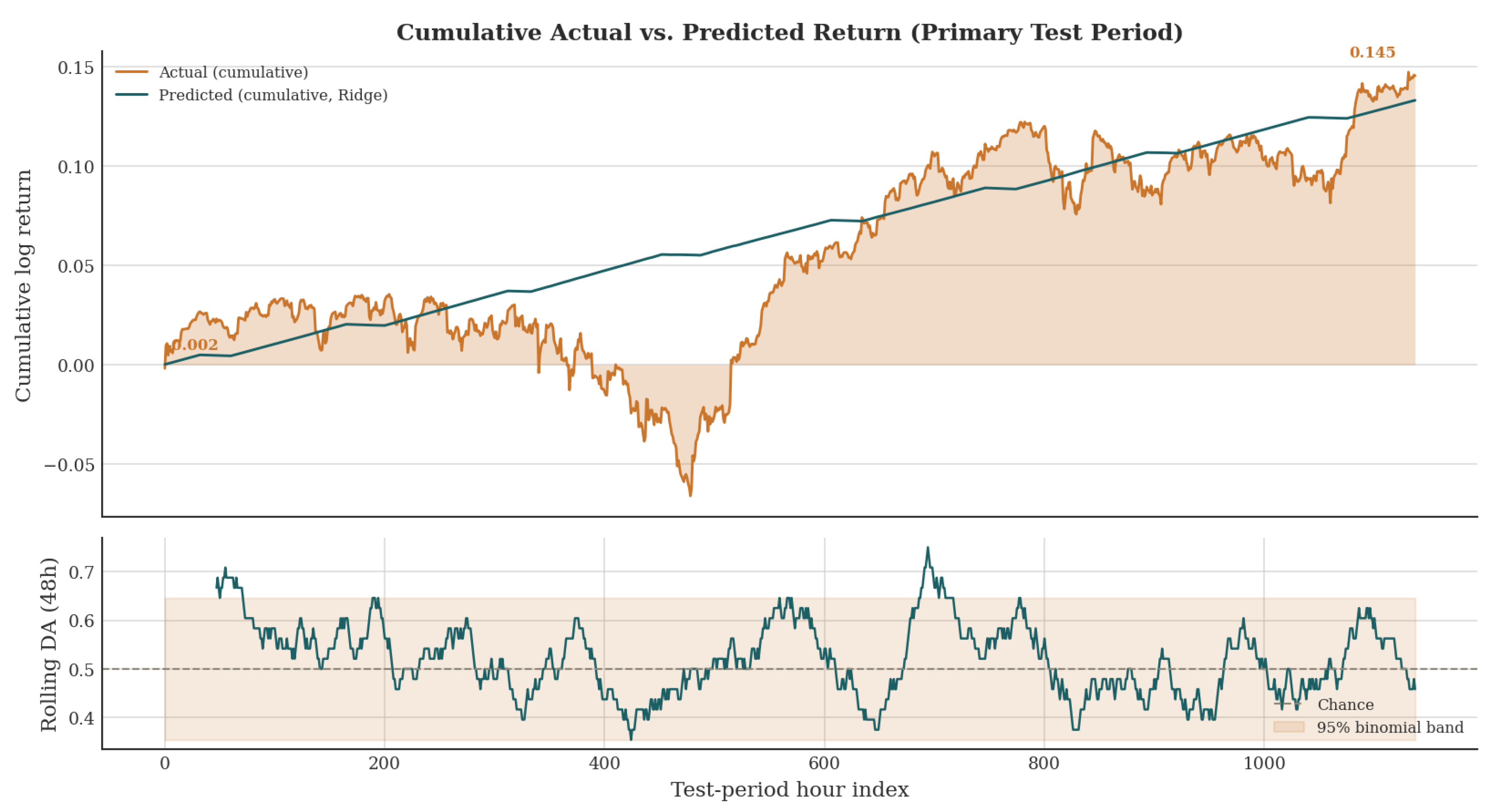
Figure 2.
Ridge cumulative in-sample fit (training) vs. out-of-sample forecast (test), with rolling absolute error.
Figure 2.
Ridge cumulative in-sample fit (training) vs. out-of-sample forecast (test), with rolling absolute error.
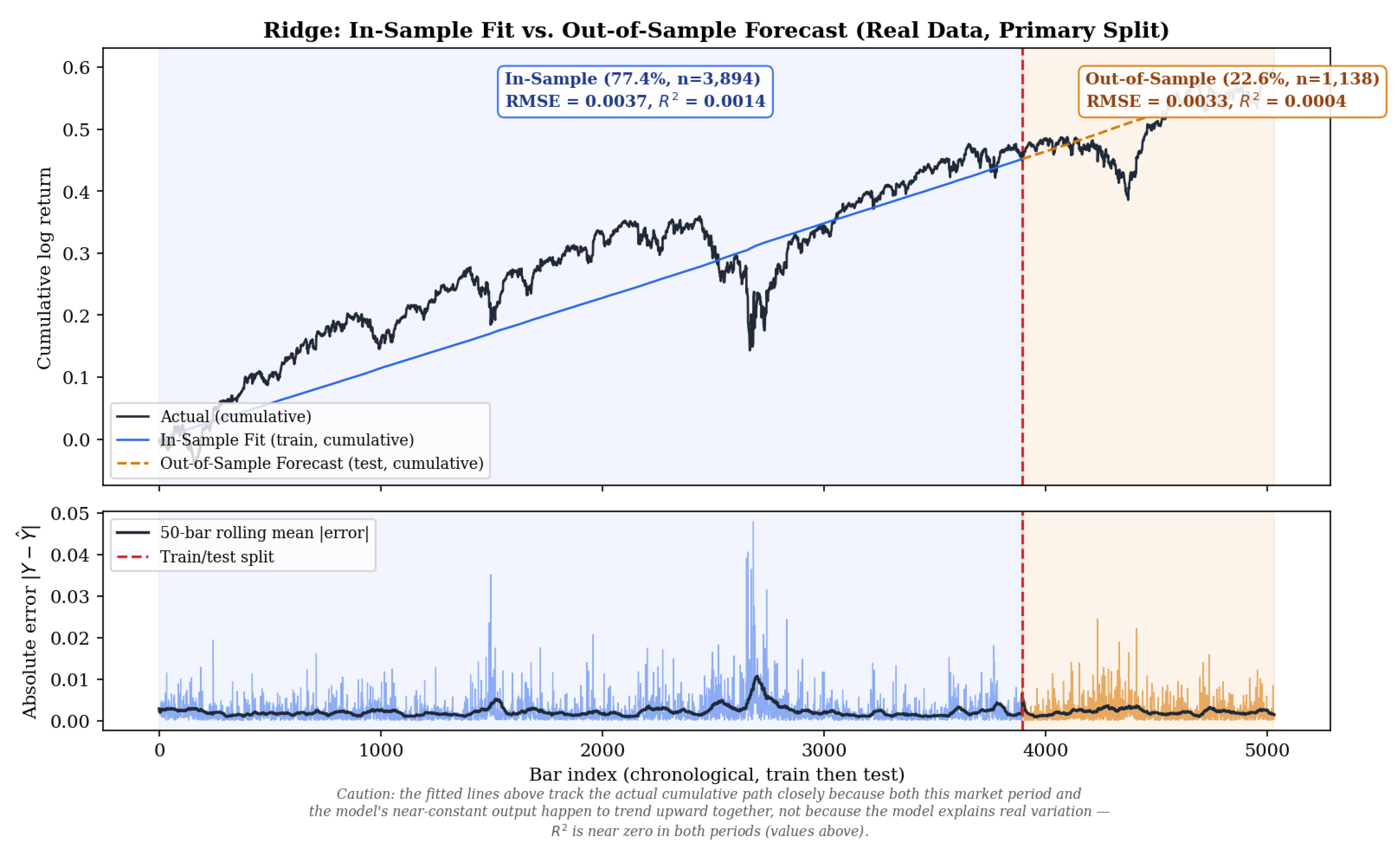
Figure 3.
RMSE vs. CCC for all baselines, MALP-Meta variants, and strategies; point size encodes DA.
Figure 3.
RMSE vs. CCC for all baselines, MALP-Meta variants, and strategies; point size encodes DA.
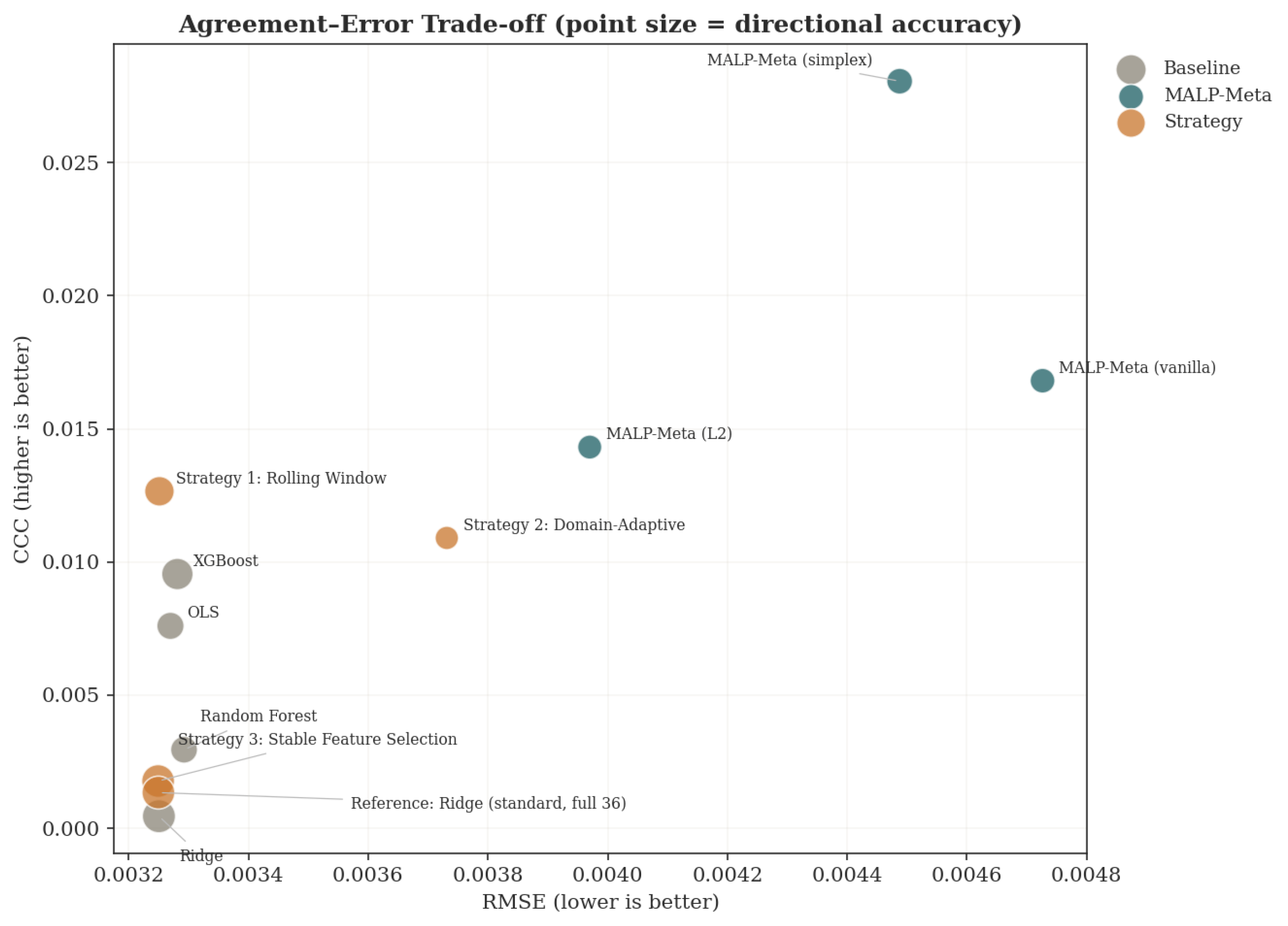
Figure 4.
CCC decomposed into Pearson correlation r and bias-correction () for each baseline.
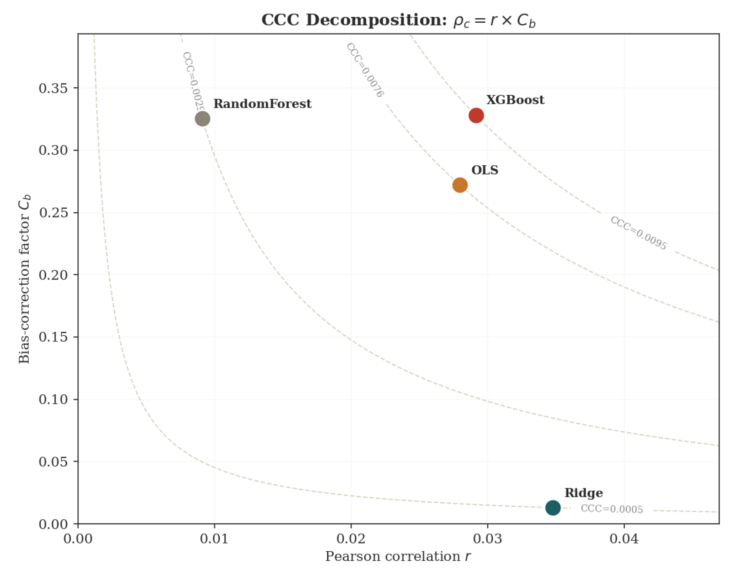
Figure 5.
Performance heatmap: all baselines, MALP-Meta variants, and strategies, six metrics.
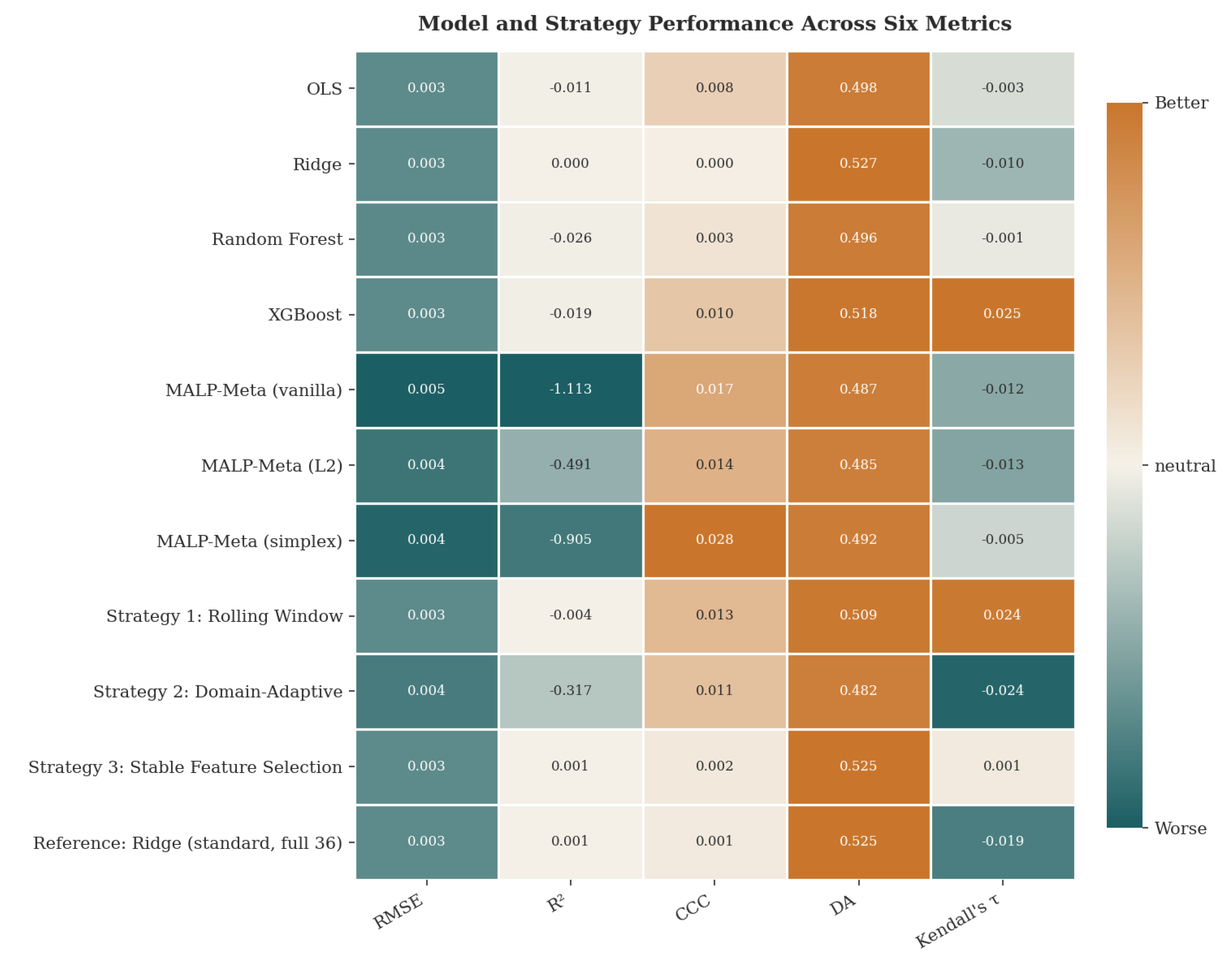
Figure 6.
Simplex MALP-Meta stress-regime forecast, directional hit/miss strip, rolling DA, and sign-alignment quadrants (pooled VIX>25 hours).
Figure 6.
Simplex MALP-Meta stress-regime forecast, directional hit/miss strip, rolling DA, and sign-alignment quadrants (pooled VIX>25 hours).
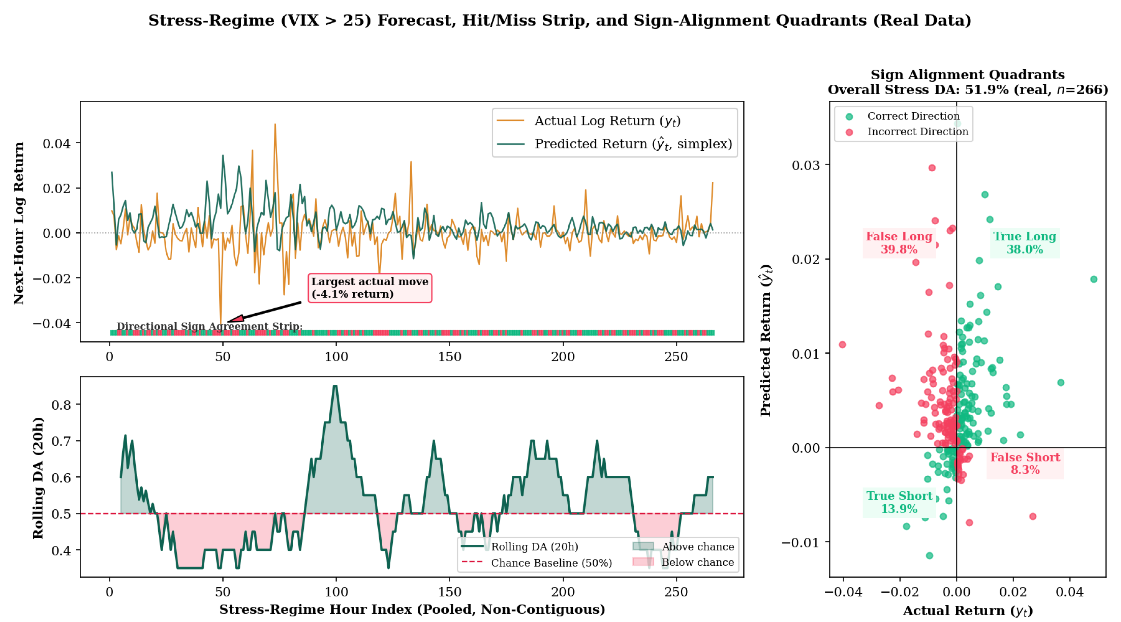
Figure 7.
Directional accuracy and significance strength across the split-point sensitivity sweep.
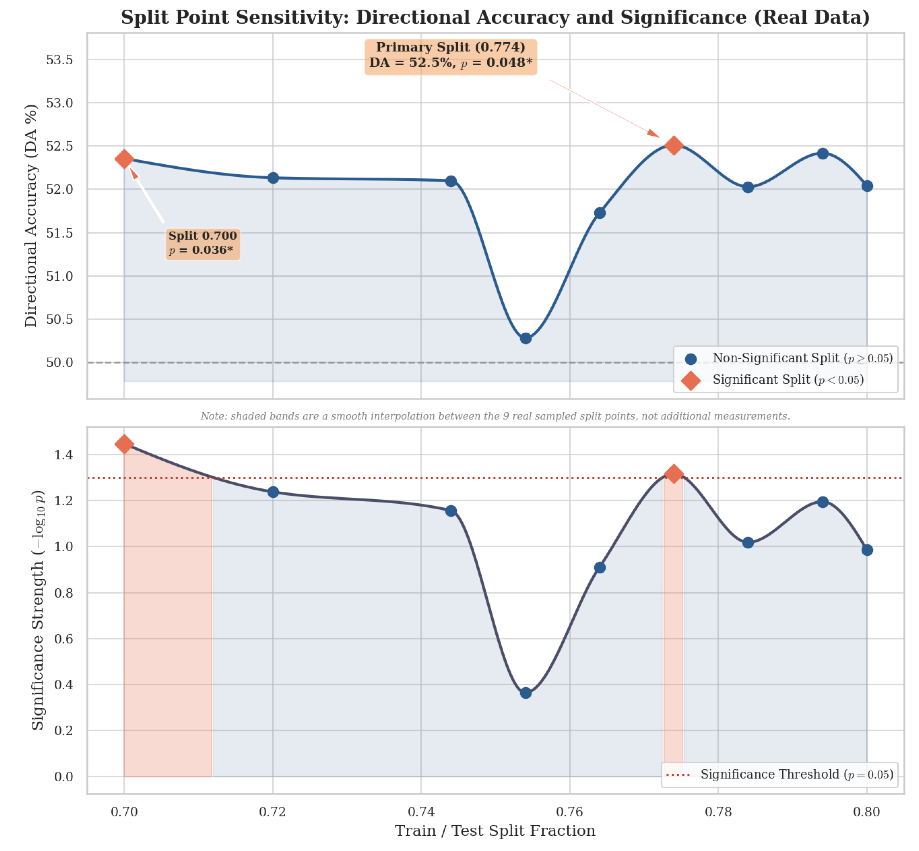
Figure 8.
Agreement-Based Permutation Importance, top 15 features by absolute CCC impact.
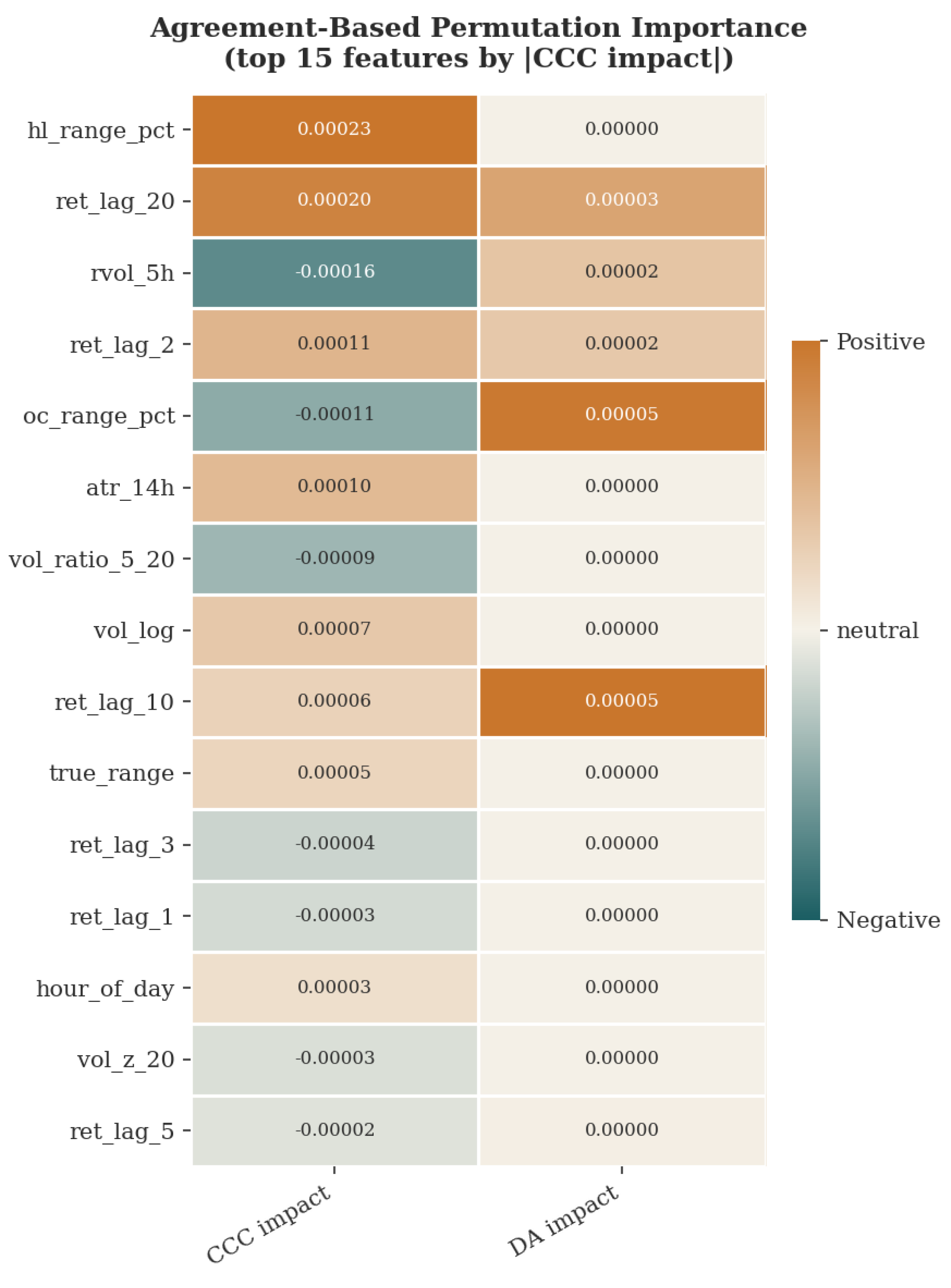
Figure 9.
Accumulated Local Effects for the four highest-attribution features.
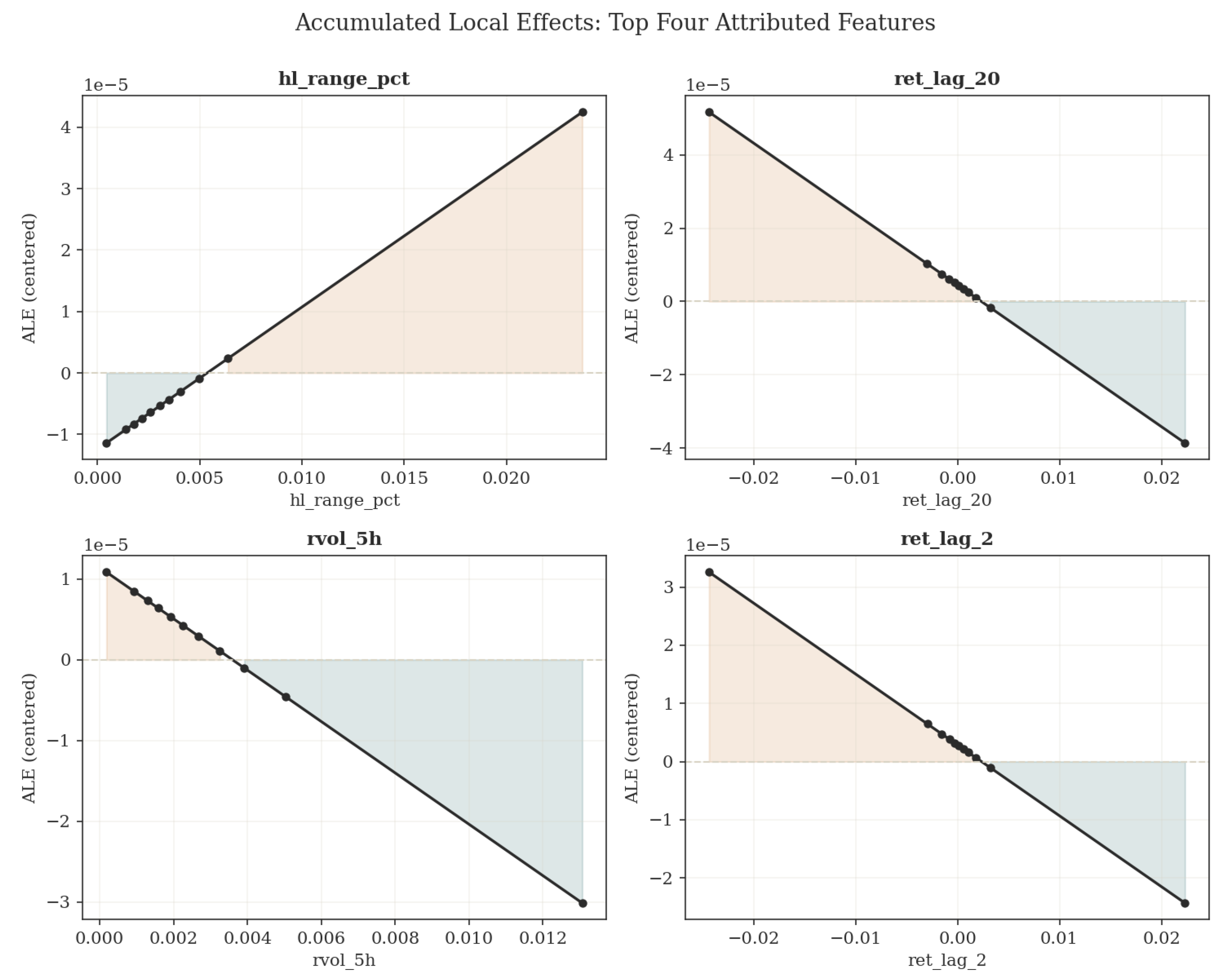

Table 1.
Summary of Related Work: Convergence and Gaps Relative to This Study
| Research Stream | Representative Works | Convergence with This Study | Gap This Study Addresses |
|---|---|---|---|
| Classical error-based forecasting | Hyndman Athanasopoulos [11]; Hoerl Kennard [12]; Tibshirani [13] | Provides our four base learners (OLS, Ridge, RF, XGBoost) and the MSE benchmark against which agreement-based optimization is evaluated | Does not address directional consistency; optimizes a criterion (MSE) misaligned with decision-relevant accuracy |
| Concordance correlation / MALP theory | Lin [5]; Kim et al. [3], Kim et al. [4]; Wadoux Minasny [18] | Supplies the CCC objective and the MALP estimator that our meta-learner directly optimizes | Established only for stationary, low-dimensional, single-model settings; behavior under temporal shift and as an ensemble meta-learner is untested |
| Concept drift / temporal shift | Gama et al. [7]; Zhang et al. [8]; Liu et al. [9]; Fan et al. [10]; Kim et al. [21] | Supplies the taxonomy (temporal shift vs. concept drift) and adaptation techniques (reweighting, normalization, domain adaptation) we adapt as robustness strategies | Exclusively targets error-minimization objectives; robustness of agreement-based optimization under shift is unexamined |
| Equity market forecasting and efficiency | Fama [24]; Gu et al. [25]; Krauss et al. [26] | Motivates the empirical domain, the near-efficient-market expectation of small real effects, and the emphasis on independent validation (Section 8) | Documents modest, hard-to-detect predictability in equity markets but does not connect this to agreement-based or feature-stability methods |
Table 2.
Baseline Model Performance on Primary Test Set
| Model | RMSE | MAE | CCC | DA | Kendall’s | |
|---|---|---|---|---|---|---|
| OLS | 0.0033 | 0.0021 | 0.0076 | 0.4978 | ||
| Ridge | 0.0033 | 0.0021 | 0.0004 | 0.0005 | 0.5269* | |
| Random Forest | 0.0033 | 0.0021 | 0.0265 | 0.5022 | 0.0104 | |
| XGBoost | 0.0033 | 0.0021 | 0.0176 | 0.5233 | 0.0307 |
*, one-sided binomial test against DA (, 598 correct, ).
Table 3.
Ablation Study: Three Arms
| Model | RMSE | CCC | DA | |
|---|---|---|---|---|
| Arm A: Meta-learner vs. equal-weight average | ||||
| Equal-weight average | 0.0033 | 0.0052 | 0.5137 | |
| MALP-Meta (simplex) | 0.0045 | 0.0281 | 0.4916 | |
| Arm B: Pruned (25) vs. full (36) features | ||||
| Random Forest, pruned | 0.0033 | 0.0028 | 0.4996 | |
| Random Forest, full | 0.0033 | 0.0265 | 0.5022 | |
| XGBoost, pruned | 0.0033 | 0.0095 | 0.5181 | |
| XGBoost, full | 0.0033 | 0.0176 | 0.5233 | |
| Arm C: Leave-one-base-model-out (simplex) | ||||
| Drop Ridge | 0.0045 | 0.0281 | 0.4925 | |
| Drop Random Forest | 0.0045 | 0.0282 | 0.4960 | |
| Drop XGBoost | 0.0045 | 0.0276 | 0.4899 | |
Table 4.
Temporal Robustness Strategies. Reference is Ridge, full 36-feature set (distinct from Table 2’s pruned-25 Ridge).
Table 4.
Temporal Robustness Strategies. Reference is Ridge, full 36-feature set (distinct from Table 2’s pruned-25 Ridge).
| Strategy | RMSE | CCC | DA | p-value | |
|---|---|---|---|---|---|
| Reference: Ridge (full 36 features) | 0.0032 | 0.0009 | 0.0013 | 0.5251 | 0.048* |
| Strategy 1: Rolling Window | 0.0033 | 0.0127 | 0.5085 | 0.295 | |
| Strategy 2: Domain-Adaptive | 0.0037 | 0.0109 | 0.4819 | 0.894 | |
| Strategy 3: Stable Feature Selection | 0.0032 | 0.0012 | 0.0018 | 0.5251 | 0.048* |
*, one-sided binomial test against DA .
Table 5.
Top 15 Features by Composite Selection Score
| Feature | Importance | Stability | Composite Score |
|---|---|---|---|
| mom_10h | 0.0452 | 0.9590 | 0.0433 |
| mom_40h | 0.0347 | 0.9666 | 0.0336 |
| rvol_5h | 0.0328 | 0.9823 | 0.0322 |
| ret_lag_5 | 0.0322 | 0.9876 | 0.0318 |
| vol_log | 0.0312 | 0.9984 | 0.0312 |
| ret_lag_10 | 0.0310 | 0.9972 | 0.0309 |
| mom_20h | 0.0308 | 0.9995 | 0.0308 |
| hl_range_pct | 0.0311 | 0.9729 | 0.0303 |
| ret_lag_20 | 0.0312 | 0.9596 | 0.0299 |
| rvol_20h | 0.0303 | 0.9829 | 0.0298 |
| atr_14h | 0.0348 | 0.8087 | 0.0281 |
| macd | 0.0354 | 0.7817 | 0.0277 |
| vol_ratio_5_20 | 0.0271 | 0.9920 | 0.0268 |
| rvol_10h | 0.0270 | 0.9809 | 0.0265 |
| macd_signal | 0.0331 | 0.7976 | 0.0264 |
Disclaimer/Publisher’s Note: The statements, opinions and data contained in all publications are solely those of the individual author(s) and contributor(s) and not of MDPI and/or the editor(s). MDPI and/or the editor(s) disclaim responsibility for any injury to people or property resulting from any ideas, methods, instructions or products referred to in the content. |
© 2026 by the authors. Licensee MDPI, Basel, Switzerland. This article is an open access article distributed under the terms and conditions of the Creative Commons Attribution (CC BY) license (http://creativecommons.org/licenses/by/4.0/).
Copyright: This open access article is published under a Creative Commons CC BY 4.0 license, which permit the free download, distribution, and reuse, provided that the author and preprint are cited in any reuse.