

Submitted:
29 August 2026
Posted:
01 September 2026
You are already at the latest version
Abstract
Comprehensive wealth accounting defines net investment in natural capital as the change in the stock, yet country-level ESG research has concentrated on flow measures of environmental pressure and left this outcome unexamined. Drawing on the World Bank Sovereign ESG Data Portal, this paper takes the annual change in renewable natural capital per capita, from the Changing Wealth of Nations accounts, as its dependent variable, for 149 to 151 countries between 1995 and 2020. It is explained three times, through parallel equations differing only in the ESG pillar of origin of their regressors, so that the three sets of determinants are estimated as distinct and comparable effects rather than compressed into a composite index. Each equation is developed through panel econometrics across six estimators, a comparison of six clustering algorithms ranked on eleven internal validity indices, and six supervised learners used to validate the specification rather than to predict. Median renewable natural capital per capita falls by 29.7 per cent and its share of comprehensive wealth halves, yet the aggregate stock is roughly constant: the coefficient on population growth is −0.913, indistinguishable from the value implied by the accounting identity, and becomes insignificant on the total stock. The decline is therefore demographic arithmetic. Climatic stress is the most robust environmental determinant, and its coefficient more than doubles when agricultural land is excluded from the dependent variable. Institutional trajectory dominates institutional level, a distinction recovered independently by the clustering. Relationships differ systematically between the two panel dimensions, and the renewable energy share reverses sign across them.
Keywords:
renewable natural capital
; comprehensive wealth accounting
; environmental investment
; ESG
; Sovereign ESG Data Portal
; weak sustainability
; panel data econometrics
; clustering
; machine learning validation
1. Introduction
Comprehensive wealth accounting defines an economy as sustainable when the value of its total capital stock, produced, human and natural, is not declining per head, and the change in that stock is therefore the operational measure of whether a country is investing in or liquidating its future (Dasgupta, 2009; Polasky et al., 2015). Three decades of measurement work have made the concept operational: wealth accounts have been compiled, extended to omitted assets and adapted to technological progress and ageing populations (Ahmad et al., 2018; Yamaguchi, 2014; Biasi et al., 2019). The picture is consistent: natural capital per capita is falling across most of the world.
What this literature has not produced is an account of why. The change in the natural asset base is treated as an accounting outcome, obtained by subtracting depletion from investment within a savings identity, rather than as a phenomenon with determinants to be estimated (Boos, 2015; Engelbrecht, 2016). A quarter of a century of estimates therefore exists without an explanation of the variation it contains.
A second literature applies environmental, social and governance frameworks at country rather than firm level, and has grown rapidly around the World Bank Sovereign ESG Data Portal. Its dependent variables, however, are almost invariably flows: emissions, energy consumption, the ecological footprint (Ibrahim & Ajide, 2022; Jahanger et al., 2023; Kılıçaslan et al., 2025). These measure the rate at which damage is done rather than the stock it draws down, and the distinction matters, since a country can reduce emissions while converting forest to cropland. That literature also aggregates the three pillars into composite scores with conventional weights, a practice whose interpretive difficulties are documented but persistent (Cook & Davíðsdóttir, 2021; Hoekstra, 2020).
The two literatures therefore speak past one another. One measures environmental wealth without explaining it; the other explains environmental pressure without measuring wealth. This paper occupies the gap between them and asks a single question: which environmental, social and governance conditions are associated with a country adding to, rather than drawing down, its stock of natural assets?
The originality of the answer lies as much in the architecture as in the variable. The dependent variable is the annual change in renewable natural capital per capita, drawn from the Changing Wealth of Nations accounts within the Sovereign ESG portal, for 149 to 151 countries between 1995 and 2020. It is explained three times, through three parallel equations differing only in the pillar of origin of their regressors, so that environmental, social and governance determinants are estimated as distinct and directly comparable effects rather than compressed into an index with arbitrary weights. Each equation is then developed along three routes: panel econometrics across six estimators, with the Mundlak test separating the between and within dimensions that applied work routinely conflates; a competition among six clustering algorithms ranked on eleven internal validity indices, since these criteria disagree systematically by algorithm family (Zhao et al., 2023); and six supervised learners deployed not to predict but to validate the specification through permutation importance, Shapley values and partial dependence. The design yields nine analytical modules on one outcome, entirely reproducible from public data, and speaks directly to the monitoring of sustainability criteria for which the change in natural capital per capita is the operational indicator.
The paper is organised as follows. Section 2 locates the study between two literatures that have developed in parallel, comprehensive wealth accounting and country-level ESG analysis, and identifies the gap between them. Section 3 describes the data and the three analytical routes. Section 4 to 12 form the empirical core: for each ESG pillar in turn — environmental, social and governance — a panel analysis across six estimators, a comparison of six clustering algorithms on eleven internal validity indices, and a machine learning module used to validate the econometric specification rather than to predict. Section 13 draws the nine modules together, Section 14 sets out the limitations, Section 15 the policy implications and Section 16 concludes. Appendices A to I report, in the same order, the full diagnostics, robustness and instrumental variable results for each of the nine modules, and Appendix J lists every variable, acronym and source code used.
2. Literature Review
The question this paper asks — which environmental, social and governance conditions are associated with a country adding to rather than drawing down its stock of natural assets — sits between two research programmes developed in parallel.
The first is comprehensive wealth accounting, built on the proposition that an economy is sustainable if its total capital stock, produced, human and natural, is not declining per head (Dasgupta, 2009; Dasgupta, 2010; Hanley et al., 2015). Its empirical branch has documented the composition of national wealth and how often countries fail that criterion (Ahmad et al., 2018; Yamaguchi, 2014; Managi et al., 2024), extended the accounts to water and soil depletion (Biasi et al., 2019), tested sensitivity to discount rates and technological progress (Yamaguchi & Managi, 2019), and applied the framework to individual economies (Agarwal & Sawhney, 2021; Kumar & Mizunoya, 2022). Since boundary extensions proceed asset by asset and are not always comparable (Halkos et al., 2018; Polasky et al., 2015; Roman & Thiry, 2016), the measured base excludes the atmosphere, groundwater and several unpriced ecosystem functions. What this literature does not do is estimate the determinants of what it measures: the change in the asset base is treated as an accounting outcome of a savings identity rather than as a phenomenon with causes to be identified.
The second programme applies ESG frameworks at country level, but its dependent variables are almost invariably flows — emissions, energy consumption, the ecological footprint (Kwilinski et al., 2026; Saba et al., 2024; Wen et al., 2024). These measure the rate at which damage is done rather than the stock it draws down: a country can cut emissions while converting forest to cropland. That literature also aggregates the three pillars into composites with conventional weights, despite an established critique of arbitrary weighting (Ciacci et al., 2020; Cook & Davíðsdóttir, 2021; Hoekstra, 2020). The two also treat time asymmetrically: wealth accounting is longitudinal in principle but often cross-sectional in application, while ESG work estimates panel relationships without asking whether the identifying variation is temporal or cross-sectional — a distinction that matters, since a fixed-effects coefficient on a variable with two per cent within-country variation does not measure what its interpretation claims.
What is known about the determinants. Within each pillar there is evidence, though directed at other outcomes. Land use change has been studied ecologically, through valuations pricing ecosystem services and tracking their loss under conversion (Pacheco et al., 2018; Souliotis & Voulvoulis, 2025; Zank et al., 2016); these are confined to single countries or biomes and unconnected to national accounts. Climatic variables enter as drivers of ecological change rather than as exogenous instruments, so the identification that meteorological exogeneity offers is unexploited. The resource curse literature relates institutions to extraction, rents, emissions and the ecological footprint (Abou Houran & Mehmood, 2023; Jahanger et al., 2023; Sun et al., 2023; Zhang et al., 2023), but its outcomes are again flows, and it treats institutional quality as a level without separating it from its trajectory. The measurement critique of the Worldwide Governance Indicators is relevant: the six are too correlated to be distinct dimensions (Langbein & Knack, 2010; Muno, 2012; Kaufmann et al., 2010). Social evidence is thinnest: population enters as a control, its role in the denominator of per capita wealth never isolated from behaviour. Two strands supply mechanisms tested below. A high renewable share signals traditional biomass dependence rather than energy transition (Alsaleh & Abdul-Rahim, 2023; Naimoğlu & Shahbaz, 2025), and Gulf migration produces population growth unattainable through fertility. Neither has been brought to bear on natural capital accumulation.
Method. Three methodological literatures inform the design. The first concerns the two dimensions of a panel. The correlated random effects formulation makes the between-country and within-country relationships separate objects and tests their equality, yet applied practice reports a single preferred estimator and treats the rest as robustness, concealing rather than examining the divergence. The recent literature on shift-share instruments is also relevant, having clarified when such instruments identify a causal effect and when they do not (Goldsmith-Pinkham et al., 2020; Borusyak et al., 2022; Borusyak et al., 2025). The second concerns supervised learning, which has entered cross-country environmental research rapidly and is used predominantly for prediction and feature ranking (Chang et al., 2024; Espoir et al., 2026; Saba & Ngepah, 2022). A smaller strand uses Shapley values and partial dependence for interpretation, though to describe a fitted model rather than to test an econometric one; using a flexible learner to validate a linear specification remains uncommon. Cluster analysis lies between the two. Algorithms are usually chosen by convention, with k-means adopted by default and k selected on one index, although internal validity criteria disagree systematically by algorithm family (Deist et al., 2018; Zhao et al., 2023). Comparing several algorithms across the full set of criteria is the practice followed here. See Table 1.
3. Data and Methodology
Every variable is drawn from a single source, the Sovereign ESG Data Portal of the World Bank, which assembles country-level indicators under the three pillars of the ESG framework. No proprietary data are used, so the estimates can be reproduced in full from a public download.
The dependent variable is taken from the Changing Wealth of Nations accounts distributed within that portal. Renewable natural capital per capita is measured in real chained 2019 US dollars and comprises eight components: agricultural land, timber, non-timber forest services, forest recreation and protection, hydropower, fisheries and mangroves. Each is valued as the discounted present value of the rents it is expected to generate, and the basis for treating the total as an element of national wealth is set out in the comprehensive wealth literature (Dasgupta, 2009; Polasky et al., 2015). The accounts exclude the atmosphere, groundwater and ecosystem functions for which no defensible shadow price exists (Biasi et al., 2019; Hoekstra, 2020), so the dependent variable describes the measured base against which sustainability is officially assessed.
The dependent variable is the annual first difference of the natural logarithm of that series, in percentage points. In wealth accounting this quantity is the net investment of a nation in its renewable natural asset base, positive when the base grows faster than population and negative when it is being liquidated per head (Hanley et al., 2015; Ahmad et al., 2018). A specification in levels was rejected because the first-order autocorrelation of the level is 0.999.
The three regressor blocks correspond to the three pillars, each with seven indicators. The environmental block covers land allocation, extraction intensity, climatic stress and the energy mix: 3,611 country-year observations, 149 countries, 1996–2020. The social block covers demographic and labour market conditions: 3,293 observations, 151 countries, 1997–2020. The governance block gives 2,629 observations on 151 countries over 2003–2020, the later start reflecting the biennial publication of the Worldwide Governance Indicators before 2002. Because those six indicators correlate between 0.73 and 0.95 and cannot be treated as distinct dimensions (Langbein & Knack, 2010; Muno, 2012), they are replaced by their first two principal components, accounting for 87.7 and 5.3 per cent of their joint variance. All three panels are close to balanced.
Each pillar equation is developed along three converging routes, applied identically so that differences between pillars are attributable to the variables rather than the treatment.
The first is panel econometrics. Six estimators are reported for every equation: pooled OLS, weighted least squares, random effects, two-way fixed effects, between and correlated random effects in the Mundlak formulation. Reporting all six is a requirement of identification rather than a ritual of robustness, since the regressors differ sharply in the share of their variation that is temporal, and the Mundlak test on the group means establishes whether the between and within relationships coincide. Standard errors are clustered by country and inference on the leading coefficients is re-assessed by a wild cluster bootstrap-t with Rademacher weights and the null imposed over 1,999 replications. Shift-share instruments are constructed where simultaneity is plausible, following recent guidance on that design (Goldsmith-Pinkham et al., 2020; Borusyak et al., 2025), and dynamic specifications are estimated by least squares with dummy variables and by the Anderson–Hsiao procedure.
The second is unsupervised classification, conducted on country averages. Six algorithms — k-means, hierarchical clustering with Ward linkage, a Gaussian mixture, fuzzy c-means, density-based clustering and an unsupervised random forest built on a permuted synthetic contrast — are compared on eleven internal validity indices and ranked by their mean rank across all eleven, since these criteria disagree systematically according to the family of algorithm being evaluated (Zhao et al., 2023).
The third is supervised learning used for validation rather than prediction. Six learners are compared out of sample on the same variation the panel estimator uses, with folds grouped by country, and the best nonlinear model is then interrogated through permutation importance, Shapley additive explanations and partial dependence, to establish whether an algorithm with no knowledge of the estimated coefficients recovers the same ordering and the same directions (Deist et al., 2018). See Figure 1.
4. Panel Analysis: The E–Environment Component
The dependent variable is the annual rate of change of renewable natural capital per capita, computed as the first difference of its logarithm and expressed in percentage points. The series is taken from the Changing Wealth of Nations accounts within the World Bank Sovereign ESG Data Portal and measured in real chained 2019 US dollars. In wealth accounting it is by construction a nation’s net investment in its renewable natural asset base. Levels were rejected: their first-order autocorrelation is 0.999.
Seven environmental regressors come from the same source: annual changes in forest area and agricultural land, net forest and total resource depletion as shares of gross national income, the drought index, log population density and the renewable share of final energy. The sample covers 149 countries over 1996–2020, 3,611 observations. See Figure 2.
The median country holds renewable natural capital worth roughly 7,100 chained 2019 dollars per inhabitant in 1995 and 4,993 in 2020, a contraction of 29.7 per cent, while its share of comprehensive wealth halves from 23.3 to 12.4 per cent. The mean annual rate of change is −1.40 per cent, 77.1 per cent of observations are negative, and 131 of 149 economies record a negative average. Disinvestment from the natural asset base is therefore the modal condition of the world economy, coexisting with the accumulation of produced and human capital — precisely the configuration the weak sustainability criterion is designed to detect. The variance structure determines what each estimator can learn. The dependent variable carries 86.0 per cent of its variation within countries, so fixed-effects estimates are identified on genuine annual adjustment. The regressors divide sharply: the changes in agricultural land and forest area and the drought index vary mostly over time, while the depletion measures, the renewable energy share and population density vary mostly across countries, the last at 0.011. Reporting six estimators is a requirement of identification, not a ritual of robustness. See Table 2.
Three coefficients survive a wild cluster bootstrap-t with the null imposed and a Bonferroni correction, and the discussion is confined to those. The largest, the change in agricultural land, is close to 1.34 in every estimator exploiting within variation, but requires qualification: agricultural land is itself 62.1 per cent of renewable natural capital, so cultivated expansion mechanically raises the valuation. Excluding that component cuts the coefficient to 0.229, still significant at five per cent — five sixths accounting, one sixth a genuine spillover. The drought index is the more informative result, being the only regressor with a strong claim to exogeneity. Positive and significant at one per cent in all six estimators, it more than doubles under the same redefinition, from 0.457 to 1.113, implying that aggregates dominated by cultivated land understate the erosion of natural wealth under drought. The third result is a sign reversal that motivates the design of the whole study. See Figure 3.
Across countries the relationship is negative, at −0.010; within countries it is positive, at +0.027, both significant at one per cent. The two dimensions measure different things. A high renewable share across 149 countries is predominantly a marker of traditional biomass use in low-income economies, which also have the fastest population growth and the most intense pressure on forests and soils, so the between coefficient captures development and demography. Within a country a rising renewable share reflects substitution of modern generation for fossil and biomass inputs, relieving pressure on the land. The Mundlak test on the group means confirms this at 71.00, and the income split shows the within effect is driven by the poorer half. The lesson is a caution against composite scores aggregating such variables with fixed weights, since a pooled coefficient would average two opposite mechanisms into a number describing neither.
The remaining four coefficients do not survive the bootstrap. The specification tests support the strategy: country effects are jointly significant, Hausman and Mundlak favour correlated random effects, serial correlation is absent, and the cross-sectional dependence detected by the Pesaran test does not disturb the surviving coefficients under Driscoll–Kraay errors. The dynamic coefficient is negative and insignificant, so accumulation carries no inertia and the static estimates can be read as complete. Appendices A.3 to A.6 report the diagnostics, the instrumental variable estimates and eight alternative specifications.
The block explains 19.1 per cent of the within-country and 34.3 per cent of the between-country variation — modest, appropriately so, since the annual change in a valuation driven by commodity prices and discount rates is not a quantity a few environmental indicators can explain in large part. It establishes that climatic conditions matter most for the non-agricultural components of natural wealth, that land conversion operates predominantly as an accounting channel whose magnitude can be quantified, and that the energy mix relates to accumulation in opposite directions across and within countries.
5. Clustering Analysis: The E–Environment Component
The panel estimates describe average relationships across a sample in which countries differ enormously in how they use their natural assets. The clustering asks whether that heterogeneity is continuous or whether countries fall into a small number of recognisable environmental configurations. Each of the 149 economies is described by its 1996–2020 average of the dependent variable and the seven environmental regressors, all standardised so that no variable dominates the distance metric. The exercise makes no use of the estimated coefficients, so any agreement with the econometrics is informative rather than mechanical, and averaging over twenty-five years removes the temporal dimension, so the classification describes permanent configurations rather than trajectories. Six algorithms are compared: k-means, hierarchical clustering with Ward linkage, a Gaussian mixture, fuzzy c-means, DBSCAN, and an unsupervised random forest whose leaf co-occurrence proximities are converted into distances. They are evaluated on eleven internal validity indices covering explained variance, the information criteria, silhouette width, cluster diameter and separation, the point-biserial correlation, Dunn, entropy, Herfindahl and Calinski–Harabasz. The number of clusters is fixed beforehand so that all six face the same problem, and the choice is not unambiguous. The silhouette peaks at k = 2, but that solution merely separates rich from poor economies. From k = 3 it is essentially flat, between 0.236 and 0.253, while the marginal reduction in within-cluster deviance falls only slightly from k = 3 to k = 4, by 116 against 119, before dropping to 82 at k = 5. Four clusters are retained on the elbow criterion and on interpretability, with the silhouette accepting rather than driving the decision. See Table 3.
The first panel covers the indices that reward compact and well-explained partitions, and on all five of them the ordering is the same: k-means first, hierarchical second, random forest last. The second panel covers the indices that evaluate the geometry of the solution and the balance of the size distribution, and there the ordering changes substantially. See Table 4.
Panel B: indices of separation and of the size distribution. Higher values are preferred for minimum separation, the Dunn index and the entropy, lower values for the maximum diameter, the Herfindahl–Hirschman index and the point-biserial correlation.
No algorithm dominates on every index, which is why the comparison rests on a mean rank. K-means is first on six of eleven, including explained variance, the silhouette and both information criteria, and its mean rank of 2.50 places it ahead of hierarchical clustering at 2.77; the two agree on most memberships. Density-based clustering shows the characteristic profile of its family, leading on separation and Dunn because it isolates a dense core and treats the periphery as noise, at the cost of nineteen unassigned countries and an explained variance of 0.192. The unsupervised random forest ranks last, with a silhouette of 0.034: its proximity metric detects dependence structures rather than compact groups. The disagreement between indices is systematic rather than random, following the algorithm family — partitional methods score on compactness, density-based on separation — and the information criteria here duplicate the explained variance rather than complementing it, so their agreement is not independent confirmation. K-means is retained. The four groups that emerge are readily interpretable and the differences between them are large. See Figure 4.
The largest group, with 77 members, contains the European economies, Japan and the middle-income countries of the former Soviet bloc and the Caribbean. It is the only group in which forest area is expanding and agricultural land contracting, with resource rents at 1.06 per cent of national income and the lowest renewable energy share at 21.6 per cent. It loses renewable natural capital per capita at 0.65 per cent a year, less than half the sample mean: these stabilising economies have completed the land-use transition.
The second, with 45 members, comprises the agricultural frontier economies of sub-Saharan Africa, South-East Asia and Central America, where cultivated land is expanding, forest contracting and the renewable share high at 60.7 per cent, reflecting traditional biomass. It loses 1.95 per cent a year. The third is small and extreme: twelve forest-rent economies — the Congo basin, Liberia, Ethiopia, Gabon, Angola — with total depletion at 19.9 per cent of national income, losing 2.49 per cent. The fourth, with fifteen members, is defined by aridity rather than extraction: its drought index is 1.69 standard deviations below the mean, the largest deviation of any cluster on any variable, and it contains the Gulf states, Iraq, Iran, Egypt and Kazakhstan, recording the fastest loss at 2.85 per cent.
This connects the classification to the econometrics. The panel estimates identified the drought index as the coefficient with the strongest claim to exogeneity; the clustering, uninformed by those estimates, isolates aridity as the sharpest discriminant in the sample and identifies that group as the one losing natural wealth fastest. Two methods sharing no assumptions converge on the same variable. The ordering, from −0.65 to −2.85 per cent, spans a range wider than any single coefficient can generate, suggesting configurations matter more than marginal effects. The partition is moderate — average silhouette 0.253, eight negative widths — so the groups are real but their boundaries gradual. Details are in Appendix B.
6. Machine Learning Validation: The E–Environment Component
The third module applies supervised learning to the environmental equation, and its purpose requires stating explicitly, because it is not the one for which these algorithms are ordinarily used. The objective is not to predict the growth of renewable natural capital per capita. Prediction would be of limited interest, since the wealth accounts are published with a lag and their future values are not a policy target. The objective is validation: to establish whether the linear fixed-effects specification of Section 4 has left structure in the data unexploited, and whether a flexible learner allowed to search freely for that structure attributes explanatory weight to the same variables, and in the same direction, as the econometric model.
The exercise is conducted on exactly the variation the fixed-effects estimator uses. The dependent variable and the seven regressors are first residualised on country and year effects by iterated demeaning, so that the learners face the same within-country, within-year information as the panel estimator and any difference in performance is attributable to functional form rather than to the treatment of heterogeneity. Six algorithms are compared: linear regression, a linear support vector machine, k-nearest neighbours with twenty-five neighbours and distance weighting, a decision tree of depth six, a random forest of six hundred trees, and gradient boosting with six hundred stages and a learning rate of 0.03. Validation uses ten-fold cross-validation with folds constructed by country, so that all observations of a given economy fall in the same fold and no learner can exploit the persistence of a country’s characteristics to predict its own future observations. The grouping is a precaution rather than a necessity in this sample, since repeating the comparison with conventional random folds leaves the ordering of the models unchanged, but it is the conservative choice and it is what makes the comparison a genuine test of generalisation to economies the learner has never seen.

Table 5.
Comparison of six supervised learners on the residualised environmental equation, 3,611 observations, ten-fold cross-validation grouped by country.
Table 5.
Comparison of six supervised learners on the residualised environmental equation, 3,611 observations, ten-fold cross-validation grouped by country.
| Model | Cross-validated R2 | RMSE | MAE | Correlation | In-sample R2 | Overfitting gap |
| Linear regression | 0.1842 | 2.851 | 1.457 | 0.429 | 0.191 | 0.007 |
| Linear SVM | 0.1791 | 2.860 | 1.422 | 0.424 | 0.181 | 0.002 |
| Random forest | 0.1399 | 2.927 | 1.519 | 0.376 | 0.493 | 0.353 |
| K-nearest neighbours | 0.1226 | 2.957 | 1.579 | 0.350 | 1.000 | 0.877 |
| Boosting | 0.1144 | 2.970 | 1.562 | 0.363 | 0.538 | 0.423 |
| Decision tree | 0.0936 | 3.005 | 1.575 | 0.323 | 0.185 | 0.092 |
Note. The overfitting gap is the difference between the in-sample and the cross-validated coefficient of determination.
The ordering is unambiguous and is the opposite of what a prediction-oriented exercise would hope for. Linear regression achieves the highest cross-validated coefficient of determination at 0.1842, followed closely by the linear support vector machine at 0.1791. The random forest reaches 0.1399, k-nearest neighbours 0.1226, boosting 0.1144 and the single tree 0.0936. The final two columns explain why. The flexible learners fit the training data far better than the linear model, with in-sample coefficients of 0.493 for the random forest and 0.538 for boosting against 0.191 for the linear specification, and k-nearest neighbours with distance weighting interpolates the training data exactly, but none of this additional fit generalises to countries not seen during training. The gap between in-sample and out-of-sample performance is 0.007 for linear regression and between 0.35 and 0.88 for the flexible learners.
The conclusion is a validation result of the strongest kind available in this design. When six learners of very different inductive bias are given the same information, the linear specification is not merely competitive but best, which means the econometric model of Section 4 is not discarding systematic structure that a more flexible functional form could recover. Two direct tests confirm the reading. Adding all twenty-one pairwise interactions to the linear model reduces cross-validated performance from 0.1842 to 0.1794, and adding the seven squared terms leaves it essentially unchanged at 0.1843; including both together reduces it further to 0.1758. Neither non-linearity nor interaction is present in a form that survives out-of-sample validation.
Establishing that flexibility does not help is only half of the validation. The second half asks whether a flexible learner, when allowed to allocate explanatory weight freely, allocates it to the same variables as the panel estimator. The random forest is used for this purpose, being the best performing of the non-linear learners, and its attribution is computed through permutation importance and through Shapley additive explanations. Figure 5.
The agreement is close. The three regressors that survived the bootstrap in Section 4 are those to which the random forest assigns most weight, in the same order: the change in agricultural land takes 45.2 per cent of the total mean absolute SHAP value, the drought index 23.2 per cent and the renewable energy share 8.1 per cent, together 76.5 per cent of the attributed explanation. The four that failed the bootstrap receive between 4.7 and 7.1 per cent each, close to what an uninformative variable receives among seven. The Spearman correlation between the SHAP ranking and the ranking by absolute standardised coefficient is 0.750, and 0.857 for permutation importance. Direction agrees where the econometric model makes a claim. For the three significant regressors the correlation between a variable and its SHAP contribution is positive throughout, at 0.951, 0.847 and 0.511, matching the fixed-effects signs. Three of the four insignificant regressors disagree in direction, which is uninformative rather than contradictory, since a coefficient indistinguishable from zero has no sign to match. Partial dependence gives the same answer differently. The curve for agricultural land is almost a straight line, a linear fit accounting for 96.7 per cent of its variation with a slope of 1.50 against a coefficient of 1.34; the drought index yields 0.914 and a slope of 0.385 against 0.457. Only the renewable energy share shows appreciable curvature, at 0.540: flat over the lower range and rising thereafter, consistent with a threshold below which substitution of modern generation has little effect on land pressure. This is the one respect in which the module refines rather than confirms the specification. Three limitations follow from what the exercise is. Attribution is not identification: a SHAP value measures how a variable moves a fitted prediction, not the outcome under intervention. The learners receive the same seven regressors, so no omitted variable can be revealed. And residualisation removes the cross-country variation, so the sign reversal on the renewable energy share is invisible here by construction. Remaining diagnostics are in Appendix C.
7. Panel Analysis: The S–Social Component
The second equation retains the dependent variable of Section 4, the annual rate of change of renewable natural capital per capita, and replaces the environmental regressors with the social block of the Sovereign ESG framework. Seven indicators are used: the rate of population growth, the total fertility rate, the annual change in life expectancy at birth, the labour force participation rate, the ratio of female to male participation, the annual change in the share of the population with access to electricity, and the share of parliamentary seats held by women. The estimation sample covers 151 countries between 1997 and 2020, for 3,293 country-year observations. Collinearity is low, with variance inflation factors between 1.01 and 1.92; the correlation of 0.59 between fertility and population growth is the highest in the block and is well within tolerance.
One feature of this equation requires treatment before any coefficient is interpreted, and it is the social analogue of the accounting problem addressed in Section 4.6. The dependent variable is a per capita magnitude, so population growth enters it through the denominator by construction: the growth of renewable natural capital per capita is identically the growth of the total stock minus the rate of population growth. A coefficient of −1 on population growth is therefore what the accounting identity predicts before any behavioural mechanism is considered. Population growth nonetheless belongs to the social pillar in the World Bank classification and cannot simply be omitted, so the strategy adopted here is to include it, to test whether its estimated coefficient departs from the identity value, and to re-estimate the entire equation with the growth of the total stock as the dependent variable, in which specification population growth has no mechanical role at all. See Table 6.
The coefficient on population growth is the most stable estimate in this study. It ranges from −0.818 to −0.995 across the six estimators and is significant at the one per cent level in every one of them, and in four of the six the confidence interval contains −1. This is precisely the identity value, and it is the first indication that the relationship is arithmetic rather than behavioural. The between estimator, at −0.994 with a standard error of 0.054, is indistinguishable from the identity to two decimal places.
The decisive test is the change of dependent variable, and its result is unambiguous. See Figure 6.
Over the estimation sample the mean growth of renewable natural capital per capita is −1.37 per cent a year, that of the total stock +0.07 per cent, and mean population growth 1.43 per cent. The per capita decline is therefore demographic: the world’s renewable asset base has been approximately constant in aggregate, and 89 of the 151 countries record a non-negative average change in the total stock against only 20 in per capita terms. Re-estimating on total growth moves the coefficient on population growth from −0.913 to +0.087 (p = 0.306), and in the cross-section the slope reverses outright, from −0.877 to +0.123. Countries with faster population growth are not depleting their asset base more rapidly; they are dividing a roughly constant base among more people. The decline documented in Section 4 is thus not primarily a story of environmental mismanagement but of demography operating on a stock that is not growing. Two qualifications apply: the valuation is a discounted rent, so a constant total may conceal offsetting movements in quantities and prices, and the accounts omit the atmosphere and subsoil water.
One social variable survives the change of dependent variable. The fertility coefficient is 0.537 on both definitions (p = 0.008), so it is not an artefact of the denominator, and decomposing by component locates the mechanism: 0.975 on agricultural land (p = 0.0003) and −0.033, insignificant, on everything else. Higher fertility is associated with the expansion of cultivated land and nothing else, a Boserupian pattern in which the accounts register the conversion of one natural asset into another as an increase. The remaining five regressors are weak.
The diagnostics differ sharply from the environmental block. Country effects are jointly insignificant (F = 0.709, p = 0.997), the Hausman test does not reject random effects, and the Mundlak test is borderline at 0.058, because population growth absorbs the heterogeneity the country effects would otherwise capture. The between estimator explains 82.0 per cent of the cross-country variation against 34.3 per cent for the environmental block, and only 5.5 per cent within. The dynamic coefficient, −0.201, indicates mean reversion. Instrumentation is informative here because fertility is a candidate for simultaneity: a shift-share instrument with a first-stage F of 155.6 returns 0.540 against 0.537, with a Wu–Hausman p-value of 0.991. Applied to population growth the same design is weak (F = 6.2) and would instrument an identity; it is reported in Appendix D.
8. Clustering Analysis: The S–Social Component
The social equation of Section 7 reached a conclusion that is arithmetic in nature: the decline of renewable natural capital per capita is almost entirely the effect of population growth operating on a stock that is roughly constant in aggregate. That conclusion holds on average, and the natural follow-up question is whether the demographic configurations producing it are homogeneous across the world or whether distinct national types can be identified. This is the question the clustering module addresses. As in Section 5 the unit of analysis is the country, described by the average over 1997–2020 of the dependent variable and of the seven social regressors, all standardised before clustering; and as in Section 5 the exercise makes no use of the estimated coefficients, so any agreement with the econometric results is informative rather than mechanical.
Before the results are read, one restriction of the design should be recalled from Section 5. Averaging over twenty-four years removes the temporal dimension, so the classification describes permanent national configurations rather than trajectories. In the social block this restriction is more consequential than in the environmental one, because several of the variables are moving systematically over the period: fertility falls in most developing economies, life expectancy rises almost everywhere, and access to electricity expands. A country is therefore placed according to its average position along a transition that it is traversing, not according to where it now stands. The classification should be read as a typology of demographic regimes over the last quarter of a century, and the groups identified below would be drawn differently on data from 2020 alone.
The same six algorithms are compared on the same eleven internal validity indices. The number of clusters is fixed at four, and here the criteria agree rather than conflict. The average silhouette width attains its maximum over the whole range from two to ten precisely at k = 4, at 0.344, and falls sharply thereafter, to 0.220 at k = 6. Explained variance reaches 0.515 and the marginal reduction in within-cluster deviance, having fallen from 178.5 at k = 3 to 76.5 at k = 4, declines only gradually afterwards. The absence of the tension that characterised the environmental block is itself a result: the social variables partition the world more cleanly than the environmental ones, and the average silhouette of the retained solution, at 0.344, exceeds the 0.253. See Table 7.
K-means is again the preferred algorithm, and by a wider margin than in the environmental block: its mean rank of 2.18 rests on first place in eight of the eleven indices, including explained variance, the silhouette, both information criteria, the maximum diameter and the point-biserial correlation. Hierarchical clustering follows at 2.45 and produces a broadly similar partition. Two differences from Section 5 deserve note. The unsupervised random forest performs considerably better here, moving from last place with a silhouette of 0.034 to fourth with 0.272, which suggests that the social variables contain the kind of dependence structure its proximity metric is designed to detect. Model-based clustering performs considerably worse, falling to fifth with a silhouette of 0.128, because the Gaussian mixture with unrestricted covariance fits elongated overlapping components to what are in fact compact groups of unequal size. The second panel of indices, reported in Appendix E, confirms that density-based clustering again buys separation at the price of coverage, leaving 42 countries unassigned. See Table 8.
The four groups are more sharply differentiated than their environmental counterparts, and the ordering of their rates of natural capital accumulation is far wider. See Figure 7.
The largest group, with 79 members, comprises Europe, North America, China, the former Soviet republics and the Southern Cone. Fertility averages 1.84 births per woman and population growth 0.54 per cent, and these economies lose renewable natural capital per capita at 0.62 per cent a year, the slowest rate in the classification: demographically settled. The second group, with 40 members, is sub-Saharan Africa almost in its entirety — fertility 4.94, population growth 2.51 per cent, the highest female participation of the four — and loses 2.07 per cent a year. The third, with 26 members, spans North Africa, the Middle East, South Asia and parts of Central America, and is defined not by fertility but by the exclusion of women from the labour market, with participation 1.50 standard deviations below the sample mean. It loses 1.95 per cent a year, almost identical to the African group: two very different social configurations produce the same environmental outcome. The fourth group has six members — Bahrain, the United Arab Emirates, Qatar, Kuwait, Oman and the Maldives — and is the most extreme observation in the paper. Population growth averages 4.69 per cent a year while fertility, at 2.27, is below the sample average, a combination possible only through immigration, and natural capital per capita falls at 5.08 per cent a year. Were the decline driven by environmental behaviour, the most extreme group should be distinguished by extraction or land conversion; instead it is distinguished by migration. The clustering, given no information about the accounting identity of Section 7, recovers it as the defining feature of the extreme case. The ordering, from −0.62 to −5.08 per cent, spans a range four times wider than the environmental classification, and almost all of it is demographic. A reader treating the ranking as a league table of environmental performance would be reading population growth rates — the sense in which composite ESG scores can invert the meaning of what they aggregate. The average silhouette is 0.344, with four negative widths. Details are in Appendix E.
9. Machine Learning Validation: The S–Social Component
The validation module is applied to the social equation in the same form as in Section 6 and with the same purpose, which is not prediction but the assessment of whether the linear panel specification has exhausted the information in the data and whether a flexible learner independently attributes explanatory weight to the same variables. The dependent variable and the seven social regressors are residualised on country and year effects before estimation, so that the learners face exactly the variation the fixed-effects estimator uses, and cross-validation is performed on ten folds constructed by country. The same six algorithms are compared.
The social equation, however, poses a question the environmental one did not, and the module is organised around it. Section 7 established that the coefficient on population growth is an accounting identity and that the substantive content of the block reduces to the fertility rate. The exercise is therefore run twice, once with the growth of renewable natural capital per capita as the dependent variable and once with the growth of the total stock, in which the identity is absent. Comparing the two runs isolates how much of the apparent explanatory power of the social block is arithmetic. See Table 9.
The pattern of Section 6 recurs and is if anything sharper. The two linear models occupy the first two places, separated by 0.0004 and effectively tied, while the three tree-based learners and the nearest-neighbour method fall behind. Gradient boosting achieves a negative cross-validated coefficient of determination, which means that predicting the sample mean for every observation would have been more accurate than the model it fitted. The overfitting gaps are large: 0.395 for the random forest and 0.485 for boosting, against 0.002 and 0.004 for the two linear specifications. Extending the linear model does not help either, and here it actively harms: adding the twenty-one pairwise interactions reduces cross-validated performance from 0.0516 to 0.0130 and adding the seven squared terms reduces it to 0.0360. Flexibility of any kind is penalised.
The absolute level of these figures should be read against the panel results rather than against Section 6. The two-way fixed-effects estimator reported a within-country coefficient of determination of 0.055 for the social block, and the best learner recovers 0.052 out of sample. The econometric model was therefore already extracting essentially all the systematic within-country signal available, and there is none left for a flexible functional form to find. That is the validation result, and it holds even though the amount of signal is small.
The attribution exercise, conducted with the random forest as the best performing non-linear learner, is where the two runs diverge instructively. See Figure 8.
With the per capita dependent variable, population growth receives 38.3 per cent of the total mean absolute SHAP value, three times any other regressor, while the remaining six divide the residual almost equally, between 9.1 and 12.8 per cent. The learner has recovered the accounting identity: given seven variables and no prior information, it concentrates the explanation on the one entering the dependent variable by construction. Fertility, the only substantive survivor of the econometric analysis, receives 9.9 per cent, indistinguishable from variables the panel found insignificant.
With the total dependent variable population growth falls to 15.6 per cent, close to the 14.3 per cent equal division would imply, and fertility rises to first at 18.6 per cent. The ordering now matches the econometric one but is close to uninformative: every regressor lies between 10.9 and 18.6 per cent, and the model explains almost nothing, with a cross-validated coefficient of 0.0006 for the linear specification and −0.020 for the random forest.
This qualifies the fertility result of Section 7. That coefficient remains significant, robust to the bootstrap and unchanged under instrumentation, but carries almost no predictive content: knowing a country’s fertility rate and six other social indicators does not predict whether its asset base will grow next year. Significance and out-of-sample relevance are separate properties, and the explanatory power of the per capita equation, at 0.052, is mostly arithmetic.
Three restrictions bound this negative conclusion. Residualisation removes the cross-country dimension, where the block was strongest (between R2 0.820 against 0.055 within); the specification is contemporaneous, whereas demographic pressure on land operates with long lags; and the dependent variable is an annual change in a discounted valuation dominated by prices no social indicator could anticipate. Where Section 6 confirmed and refined, this module confirms the specification but subtracts from the interpretation — which is what a validation exercise capable of more than one answer should do. Details are in Appendix F.
10. Panel Analysis: The G–Governance Component
The third equation retains the dependent variable of Section 4 and Section 7 and replaces the regressors with the governance block. The construction of that block requires a decision that the previous two did not, because the governance pillar of the Sovereign ESG framework is dominated by the six Worldwide Governance Indicators, and those six are not distinct measures in any statistical sense. Their pairwise correlations in this sample range from 0.73 to 0.95 with a mean of 0.85, and entering them together produces variance inflation factors up to 23.1, at which point the individual coefficients are not identified and their signs are arbitrary. See Figure 9.
The first principal component of the six accounts for 87.7 per cent of their joint variance and loads almost uniformly on all of them, between 0.374 and 0.428, so it is a general index of institutional quality rather than a contrast among its dimensions. The second component accounts for a further 5.3 per cent and is dominated by political stability, on which it loads at 0.900, against negative loadings on government effectiveness and regulatory quality; it therefore measures the extent to which a country’s stability exceeds its administrative capacity. The remaining four components together account for 7.0 per cent and are not interpretable.
The governance block is built accordingly, with seven regressors. Institutional quality is the first principal component, centred at the sample mean, and its square is included to allow the relationship to be non-monotonic, following a long-standing conjecture that environmental outcomes improve with institutions only beyond a threshold. The annual change in institutional quality is included separately, because a reform episode is a different object from a level of institutional development and, as the variance decomposition shows, it is the only governance variable with substantial year-to-year movement. The second principal component enters as the stability–effectiveness contrast. The remaining three regressors are the growth rate of GDP, the annual change in internet penetration and agriculture value added as a share of GDP. Variance inflation factors in this specification lie between 1.03 and 2.33. The sample covers 151 countries from 2003 to 2020, for 2,629 observations; the later start reflects the biennial publication of the WGI before 2002. See Table 10.
The first thing to record is the weakness of the equation in the temporal dimension. The two-way fixed-effects specification explains 0.47 per cent of the within-country variation in the accumulation of renewable natural capital per capita, against 19.1 per cent for the environmental block and 5.5 per cent for the social one. No coefficient survives the wild cluster bootstrap with the Bonferroni correction: the closest is the squared institutional quality term at a bootstrap p-value of 0.009 against a threshold of 0.00714, and the change in internet penetration at 0.028. Governance, measured annually and read within countries, does not explain the year-to-year accumulation of natural wealth. This is a negative result and it is reported as such rather than rescued by selective emphasis.
The between dimension tells a different story, and the difference is systematic rather than accidental. The between estimator explains 21.6 per cent of the cross-country variation, and two of its coefficients are significant at the one and five per cent levels respectively. Institutional quality carries 0.167, so an improvement of one standard deviation of the index, equal to 2.26 points, is associated with a rate of accumulation higher by 0.38 percentage points a year. The change in institutional quality carries 9.096, by far the largest coefficient in this study, but its magnitude reflects units: the variable is an annual change whose standard deviation across country means is 0.037, so a one standard deviation difference corresponds to 0.34 percentage points a year, and a country in the top decile of institutional improvement accumulates natural capital roughly 0.8 percentage points a year faster than one in the bottom decile. See Figure 10.
The contrast between the two panels is the substantive content of this section. Across countries the cumulative institutional trajectory over eighteen years is positively associated with the accumulation of natural wealth, with a slope of 0.231 percentage points per unit of improvement; within countries the same variable measured annually carries a slope indistinguishable from zero. The Mundlak test rejects equality of the two dimensions at 43.37, and the group-mean term on the change in institutional quality is 9.620 (p < 0.001) against a within counterpart of −0.434.
The natural reading is that institutions operate over horizons far longer than a year: improving the rule of law in a given year does not preserve more forest that year, while two decades of steady improvement leave a materially different rate of accumulation. The data cannot distinguish this from the alternative in which institutional quality marks something else, since the between dimension offers no protection against omitted permanent characteristics. The section therefore reports an association across countries and a null within them, and claims no mechanism. The squared term changes sign between dimensions, implying concavity across countries and convexity within, but it is fragile and no weight is placed on it.
The three blocks can now be compared on the same dependent variable. The environmental equation explains 19.1 per cent of the within-country variation and 34.3 per cent of the between; the social equation 5.5 and 82.0; the governance equation 0.5 and 21.6. A composite averaging the three with fixed weights would combine a variable identifying annual variation, one identifying an accounting identity and one identifying neither.
Instrumenting institutional quality returns −1.292 with a standard error of 1.342 and a Wu–Hausman p-value of 0.361: the instrument reaches only the annual component that the fixed-effects results show to be uninformative, a limitation of the design rather than a finding. Country effects are jointly significant, the Hausman and Mundlak tests reject, serial correlation is marginal, and the dynamic coefficients are negative and insignificant, so the absence of persistence found elsewhere holds here too. Details are in Appendix G.
11. Clustering Analysis: The G–Governance Component
The governance equation of Section 10 produced a result that the clustering module is well placed to examine further. Within countries, annual movements in governance explain essentially nothing about the accumulation of renewable natural capital, with a fixed-effects coefficient of determination of 0.005; across countries, the institutional trajectory over the period is associated with the rate of accumulation, and the Mundlak test rejects the equality of the two relationships decisively. Since clustering operates entirely on the cross-sectional dimension, it works precisely where the governance block has content, and the question it answers is whether the association identified econometrically corresponds to identifiable national types.
The design follows Section 5 and Section 8. Each of the 151 countries is described by the average over 2003–2020 of the dependent variable and of six governance variables: institutional quality as the first principal component of the six Worldwide Governance Indicators, its annual change, the stability–effectiveness contrast, the growth rate of GDP, the annual change in internet penetration and agriculture value added as a share of GDP. The squared institutional term used in the panel specification is omitted here, since a monotone transformation of a variable already present adds nothing to a distance metric. All variables are standardised, and the exercise makes no use of the estimated coefficients.
The number of clusters is again fixed at four, and the tension observed in the environmental block reappears in the same form. The average silhouette attains its maximum at k = 2, at 0.256, where the partition simply separates high-income from low-income economies; it then falls to 0.202 at k = 3 and recovers to 0.217 at k = 4 and 0.219 at k = 5, remaining essentially flat thereafter. The marginal reduction in within-cluster deviance falls from 119.7 at k = 3 to 81.3 at k = 4 and 57.3 at k = 5, placing the elbow at four. Explained variance at that solution is 0.453. As in Section 5 the choice rests on the elbow and on interpretability rather than on the silhouette, and the tension is recorded rather than concealed. See Table 11.
K-means obtains its clearest victory of the three blocks, with a mean rank of 1.91 built on first place in seven of the eleven indices, including explained variance, the silhouette, both information criteria, the maximum diameter and the Calinski–Harabasz statistic. Density-based clustering fails here in a way it did not in the other two blocks: its silhouette of 0.029 indicates a partition barely distinguishable from an arbitrary one, and it leaves 49 of the 151 countries unassigned, or 32.5 per cent. The reason is visible in the data rather than in the algorithm. Governance variables are close to continuously distributed across countries, with no dense regions separated by empty ones, so a method that defines clusters as regions of high density has little to find. This is itself informative about the object being classified: institutional quality is a gradient, not a set of discrete regimes. See Table 12.
The four groups are of comparable size, with a Herfindahl index of 0.266 and an entropy of 1.353, both the most balanced of the three blocks, and they divide the world along two axes rather than one. Figure 11.
The first group, with 34 members, comprises the advanced economies of Western Europe, North America, Australasia and Japan: institutional quality 1.27 standard deviations above the sample mean, agriculture at 2.3 per cent of value added. These high-capacity economies lose renewable natural capital per capita at 0.80 per cent a year. The second, with 47 members, is the mirror image — institutional quality 1.99 points below the mean, agriculture at 23.5 per cent — covering most of low-income sub-Saharan Africa with parts of Central Asia and Melanesia, and losing 2.10 per cent a year.
The remaining two are the interesting ones, because they sit at almost the same institutional level and differ sharply in outcome. The third, with 46 members, has institutional quality of 0.11 and is distinguished by improvement, with a cumulative change of +0.72 index points; it contains the Central and Eastern European accession states, the Balkans, the Caucasus, Vietnam and much of Andean South America, and loses only 0.27 per cent a year, the best outcome in the classification. The fourth, with 24 members, has institutional quality of −0.26, indistinguishable from the third, but a cumulative change of −0.28, and contains the Gulf states, Iran, Gabon, Jordan, Bolivia and Guatemala. It loses 3.11 per cent a year.
Two groups at the same institutional level, differing only in the direction of institutional travel, therefore differ in accumulation by 2.84 percentage points a year. The clustering recovers, from the cross-sectional structure alone and without any coefficient, the distinction Section 10 identified between level and change — as a property of the joint distribution rather than an average partial effect, which is weaker causally and stronger descriptively.
Two qualifications restrain this. All six migration-driven Gulf economies of Section 8 fall in the fourth cluster and constitute a quarter of its members; excluding them raises its mean from −3.11 to −2.42, so the demographic and institutional explanations overlap without either being redundant. And the partition is the weakest of the three blocks, with an average silhouette of 0.217 and the fourth group the least cohesive of all twelve clusters at 0.105. The advanced economies also record the only negative institutional trajectory among the three non-drifting groups, at −0.55, reflecting the decline registered for several Western democracies; whether that is an artefact of perception-based indices this study cannot settle. Details are in Appendix H.
12. Machine Learning Validation: The G–Governance Component
The validation module is applied to the governance equation with the same six algorithms, the same grouped cross-validation and the same purpose as in Section 6 and Section 9. The governance block, however, differs from the other two in a way that dictates the design of this section. Section 10 established that the equation has almost no temporal content, explaining 0.47 per cent of the within-country variation, and that what content it has lies in the cross-section, where the between estimator reaches 21.6 per cent and the Mundlak test rejects the equality of the two dimensions with a p-value below 0.001. Running the learners only on the residualised data would therefore test the specification exactly where the econometrics has already reported nothing. The module is consequently run twice: once on the within-transformed observations, as in the previous two blocks, and once on the 151 country means, which is the cross-sectional counterpart of the between estimator.
The asymmetry between the two runs is worth stating before the results, because it is what makes this block instructive rather than merely weak. In the environmental equation the informative dimension was temporal and the module could be run in the standard way; in the social equation the informative dimension was also temporal, though most of what it contained was an accounting identity; here it is cross-sectional. A validation exercise that applied the same residualisation to all three blocks without asking where the information lies would have concluded that the governance block is empty, when in fact it is empty only in the dimension that residualisation preserves. This is a general point about applying supervised learning to panel data: the transformation that makes the comparison fair with respect to unobserved heterogeneity also determines which of the two dimensions the learner is allowed to see, and that choice should follow the econometrics rather than convention. See Table 13.
The within columns confirm what Section 10 reported and add nothing to it. Five of the six learners return a negative cross-validated coefficient of determination, meaning that predicting the sample mean would have been more accurate than the fitted model, and the best performance, achieved by linear regression, is 0.0013. There is no signal in the annual movement of governance indicators to be recovered by any functional form, and the sharply positive overfitting gaps of the flexible learners, at 0.42 for the random forest and 0.56 for boosting, show them fitting noise. The conclusion is the same as the econometric one, reached by an independent route: governance measured annually does not explain the year-to-year accumulation of natural wealth.
The between columns produce the one exception to a pattern that has otherwise held throughout this study. See Figure 12.
In the cross-section the random forest attains a cross-validated coefficient of 0.2172 and boosting 0.2039, against 0.1291 for the linear support vector machine and 0.1090 for linear regression. This is the first and only occasion in the paper on which flexible learners outperform the linear specification out of sample, and the margin is substantial: the random forest doubles the explanatory power of the linear model. The result is not an artefact of a favourable fold assignment. Repeating the comparison across ten random partitions returns a mean of 0.288 for the random forest, with a standard deviation of 0.015, against 0.107 for the linear model with a standard deviation of 0.018, and the random forest is ahead in ten splits out of ten.
Two cautions apply before this is interpreted. The cross-section contains 151 observations, so cross-validated estimates are considerably noisier than those computed on thousands of country-year observations, and the in-sample gaps remain large, at 0.41 for the random forest and 0.79 for boosting. And the nonlinearity being exploited is not of the kind an econometrician would ordinarily add to a specification: extending the linear model with all twenty-one pairwise interactions reduces cross-validated performance from 0.109 to 0.017, and adding the seven squared terms reduces it to 0.027. Whatever structure the forest is finding, it is neither multiplicative interaction nor quadratic curvature, and the natural candidates are thresholds and local effects confined to subsets of countries — which is consistent with the taxonomy of Section 11, where four groups with distinct institutional profiles were identified and two of them differed in outcome by nearly three percentage points at almost identical institutional levels.
The attribution exercise then asks whether the forest, given the country means and no information about the econometric estimates, allocates explanatory weight in a way that matches the between coefficients. See Figure 13.
Directional agreement in the between dimension is close to complete: six of seven regressors have a SHAP direction matching the sign of the corresponding between coefficient. The three strongest correlations belong to the three variables the between estimator identified — the change in institutional quality at +0.887, its level at +0.857 and GDP growth at −0.737. The one disagreement concerns agriculture value added, whose between coefficient is zero to three decimals, so there is no sign to match.
The distribution of importance is nonetheless flat. The five leading regressors receive between 17.1 and 19.2 per cent of the total mean absolute SHAP value, close to the 14.3 per cent equal division would imply, and the rank correlation with the ordering by standardised between coefficient is accordingly low at 0.214. The learner agrees about direction and disagrees about hierarchy, which is what happens when correlated variables carry overlapping information: the forest distributes credit among them, the regression assigns it to whichever enters the linear projection most strongly. The within-dimension attribution is reported for symmetry and is uninformative, deriving from a model with negative cross-validated performance.
Partial dependence confirms the linear reading of the relationships that matter, with linear fits of 0.964 for the change in institutional quality, 0.815 for its level and 0.808 for GDP growth. The individual relationships are approximately linear, which sharpens the puzzle: the advantage of the random forest comes not from curvature in any single dimension but from the joint structure.
Three applications of the same procedure have now produced three verdicts. In the environmental equation the linear specification won and the module added a refinement; in the social equation it won and the module subtracted from the interpretation; here it loses in the dimension that matters, suggesting the econometric model is missing something. The governance block is the only one where flexibility helps, pointing to a configurational rather than marginal relationship, consistent with Section 11 and offered as interpretation rather than finding. Details are in Appendix I.
13. Discussion
The nine modules answer the same question about the same dependent variable and disagree in ways that are informative rather than contradictory. Table 14 summarises what each has established.
Read across the rows, the table shows that the three pillars occupy different positions on the same map. The environmental block is the only one that explains annual movement to any appreciable degree, because drought and land conversion are events rather than characteristics. The social block explains the cross-country ranking almost completely, at 82.0 per cent, but does so mainly through an accounting identity. The governance block explains a fifth of the ranking and none of the movement. A composite ESG score that averaged the three with fixed weights would combine a variable identifying annual variation, one identifying an identity and one identifying neither, and would report the average as a single measure of environmental performance.
Read down the columns, the methods do different work in each block, which is the strongest evidence that the design is not triangulating a foregone conclusion. Clustering converges with the econometrics twice and independently: aridity in the environmental block and the level-versus-trajectory distinction in the governance block are recovered from the cross-sectional structure alone. The machine learning module returns three different verdicts — confirming and refining, confirming and subtracting, signalling an omission — where a ratifying exercise would have returned three of the first kind.
The table also carries a lesson about where each method applies. The three do not see the same information: the panel estimators exploit both dimensions, which is why six are reported; the clustering sees only country averages; the learners see whichever dimension is preserved by the transformation. The governance block makes the consequence explicit. Residualising on country and year effects, the standard way to make a learning comparison fair with respect to unobserved heterogeneity, would have shown that block to be empty, while the same comparison on country means reveals a relationship that six learners recover and a flexible one recovers better. The choice of transformation is a decision about which question is asked, and should follow the variance decomposition rather than convention.
Two substantive conclusions follow. The first is that the global decline in natural wealth per capita is predominantly demographic rather than environmental: the aggregate stock is roughly constant over twenty-five years, and the per capita fall is arithmetic. This does not make the decline benign, since a stock that cannot grow while population does is a stock whose contribution to per capita wealth must fall, but it relocates the policy problem from environmental management to the question of whether the natural asset base can be made to grow at all.
The second is that institutional trajectory matters more than institutional level, a result that emerges independently from the between estimator, from the clustering and from the attribution exercise, and that the fixed-effects estimator cannot see. Whether the relationship is causal remains open: the between dimension offers no protection against omitted permanent characteristics, the shift-share instruments reach only the annual component, and the governance cluster losing wealth fastest overlaps by a quarter with the demographic outlier group of Section 8. What can be said is that the association is robust to three methods that share no assumptions.
Three limitations bound all of this. The estimates are associations, not causal effects: only the drought index has a strong claim to exogeneity, and the instrumental variable exercises confirm the fixed-effects results rather than establishing identification. The dependent variable is a discounted valuation, so a constant total may conceal offsetting movements in physical quantities and in prices, and the accounts omit the atmosphere, groundwater and several ecosystem functions. And the classifications average over twenty-five years, so they describe permanent national configurations rather than trajectories, a restriction that bears most heavily on the social block, where fertility and life expectancy move systematically across the period.
14. Limitations
Four sets of limitations bound what the preceding sections establish, set out in order of their consequence for interpretation.
The first concerns identification. The estimates are structural associations, not causal effects. Of the twenty-one regressors used across the three equations, only the drought index has a strong claim to exogeneity, being constructed from precipitation and evapotranspiration and not plausibly influenced by national wealth accounts. The shift-share instruments have first-stage F statistics between 6.2 and 155.6, but relevance is not sufficient, and the identifying assumptions of this design must be defended on the exposure shares rather than on the shocks (Goldsmith-Pinkham et al., 2020; Borusyak et al., 2025). In the governance block the instrument reaches only the annual component of institutional quality, which the results show to be uninformative, so it cannot speak to the cross-country association actually reported. Where a coefficient is significant, the claim is that it is a robust feature of the conditional expectation, not that intervening would move the outcome.
The second concerns the dependent variable. Renewable natural capital is a discounted valuation of expected rents, so a constant aggregate may conceal offsetting movements in quantities and prices, and the sensitivity of wealth-based measures to discount rates and to technological progress is a known weakness (Boos, 2015; Pearson et al., 2013; Engelbrecht, 2016). The accounts exclude the atmosphere, groundwater and ecosystem functions lacking a defensible shadow price, a boundary problem only partly addressed by asset-by-asset extensions (Biasi et al., 2019; Hoekstra, 2020). Agricultural land carries 62.1 per cent of the total, so the aggregate is dominated by an asset responding to agricultural support as well as to ecological condition (Ghauri et al., 2022), and Section 4.6 shows five sixths of the land-use effect to be accounting rather than economics.
The third concerns the classification and validation modules. The clustering averages over the period and describes permanent configurations rather than trajectories, a restriction bearing most heavily on the social block, where fertility, life expectancy and electricity access move systematically. Internal validity indices disagree by algorithm family, so the choice of k-means rests on a mean rank, and a different weighting of the eleven could favour another algorithm (Zhao et al., 2023). Hyperparameters were fixed rather than tuned within the cross-validation loop, so the finding that linear specifications win out of sample is defended in its weaker form: on conventional settings, flexibility does not help. The between-dimension comparison in the governance block rests on 151 observations, where cross-validated estimates are considerably noisier.
The fourth concerns coverage and measurement. The governance equation begins in 2003 because the Worldwide Governance Indicators were published biennially before 2002, and those indicators are contested as measures of distinct dimensions, being built largely from perception surveys whose correlations are too high to separate (Langbein & Knack, 2010; Kaufmann et al., 2010; Huque & Jongruck, 2018). The block therefore measures general institutional development rather than any named component. The income-based splits are descriptive rather than tests of heterogeneity, and the study covers 149 to 151 countries, excluding economies for which the wealth accounts are not compiled (Li, 2024).
15. Policy Implications
The results carry implications for three audiences, and separating them matters because the same finding points in different directions depending on the instrument available.
For the design of sovereign sustainability metrics, the implication is that composite ESG scores should not rank countries on environmental wealth. The three pillars explain very different parts of the same variation: 19.1 per cent of the within-country variation for the environmental block, 5.5 per cent but 82.0 per cent of the cross-country variation for the social block, and 0.5 and 21.6 per cent for the governance block. A fixed-weight average would combine an indicator of annual environmental events, an accounting identity and a slow-moving institutional characteristic, and report their mean as a measure of performance; the difficulty of interpreting composites built from heterogeneous series is well documented (Cook & Davíðsdóttir, 2021; Halkos et al., 2018). The sign reversal on the renewable energy share makes the point concretely: a high renewable share indicates traditional biomass dependence across countries and modern substitution within them, so a composite treating it as favourable inverts its meaning for the poorest economies (Olaniyi & Odhiambo, 2025; Naimoğlu & Shahbaz, 2025). Metrics guiding sovereign capital allocation should report the pillars separately and distinguish an indicator’s level from its trajectory.
For environmental and land policy the most robust finding is climatic. The drought index is the only regressor with a credible claim to exogeneity, is positive and significant in all six estimators, and more than doubles when agricultural land is excluded, rising from 0.457 to 1.113. The erosion of natural wealth under water stress is therefore understated by aggregates dominated by cultivated land, whose valuation is partly insulated by agricultural support. Monitoring frameworks tracking natural capital in aggregate will register drought effects late and incompletely, and disaggregated reporting by asset class is a low-cost correction, consistent with the case for spatially explicit accounting (Ahmed & Jahan, 2026; Maher et al., 2020). The land-use results point the same way: agricultural expansion raises measured natural capital while converting forest and wetland assets, so a rising aggregate may conceal a change in composition that a sustainability criterion should register.
For development policy the implication is more uncomfortable and should be stated carefully. The global decline in natural wealth per capita is almost entirely demographic: the aggregate stock is roughly constant while population grows, and the coefficient on population growth is indistinguishable from the value implied by the accounting identity. This is not an argument for population policy, and nothing here supports one; the role of population growth in wealth-based criteria is a recognised property of the accounting framework rather than a behavioural finding (Ferreira et al., 2008; Yamaguchi, 2014). It is an argument about arithmetic. If per capita natural wealth is the benchmark and the stock cannot be made to grow, the criterion will be failed by any country whose population is rising, regardless of its environmental management. Either the asset base must grow, through restoration, protection and extension of the accounting boundary to unpriced assets, or the criterion should be supplemented by measures separating stewardship from demography. The governance results suggest where effort might go: countries whose institutions improved accumulated natural capital 2.84 percentage points a year faster than countries at the same institutional level whose institutions deteriorated, and the direction of institutional change proved more informative than its level in all three methods, consistent with evidence that institutions condition the environmental consequences of resource dependence (Jahanger et al., 2023; Ameer & Ahmad, 2024).
16. Conclusions
This paper has taken the annual change in renewable natural capital per capita, which comprehensive wealth accounting defines as the net environmental investment of a nation, and estimated its determinants within an environmental, social and governance framework. The dependent variable and every regressor are drawn from the Sovereign ESG Data Portal of the World Bank, and the analysis covers 149 to 151 countries between 1995 and 2020. Three equations sharing that dependent variable and differing only in the pillar of origin of their regressors were each developed along three routes — panel econometrics across six estimators, a comparison of six clustering algorithms on eleven internal validity indices, and a comparison of six supervised learners used for specification validation rather than prediction — producing nine analytical modules on a single outcome.
Four findings emerge. The first is descriptive and reframes the others: median renewable natural capital per capita fell by 29.7 per cent over the period and its share of comprehensive wealth halved, yet the aggregate stock was roughly constant, so the per capita decline is demographic arithmetic rather than a record of environmental mismanagement. The second is that climatic conditions are the most robust environmental determinant, that the drought coefficient more than doubles when agricultural land is removed from the dependent variable, and that aridity independently defines the group of countries losing natural wealth fastest in the environmental classification. The third is that the direction of institutional change matters more than the institutional level: the between coefficient on the annual change in institutional quality is large and significant while its within counterpart is indistinguishable from zero, and the clustering recovers the same distinction from the cross-sectional structure alone. The fourth is methodological: relationships in this field differ systematically between the two dimensions of a panel, the Mundlak test rejects their equality in all three blocks, and the renewable energy share carries opposite signs across and within countries.
The design is the paper’s second contribution. Estimating the three pillars as separate and directly comparable equations, rather than aggregating them into a composite index with fixed weights, revealed that they explain different parts of the same variation, and applying the same three methods to each revealed that the methods do different work in each block. The machine learning module confirmed and refined the environmental specification, confirmed but qualified the social one by showing that its surviving coefficient carries little predictive content, and signalled an omission in the governance one by outperforming the linear model across countries. A validation procedure that could only ratify would have returned three identical verdicts.
Three directions follow. The threshold structure suggested by the renewable energy relationship and by the superior cross-sectional performance of the random forest in the governance block invites a formal threshold or finite mixture specification, which a larger cross-section could support. Extending the accounting boundary to groundwater and atmospheric assets would test whether the flat aggregate survives a fuller measure. And applying the same design to subnational wealth accounts, where the demographic denominator behaves differently, would separate stewardship from demography more cleanly than a cross-country panel allows.
Appendix A. The E–Environment Equation
The table below reports the moments of the dependent variable and of the seven environmental regressors over the estimation sample, together with the decomposition of total variation into between-country and within-country components.
Table A1.
Descriptive statistics and variance decomposition, 149 countries, 1996–2020, N = 3,611.
| Variable | Mean | SD | Min | Median | Max | SD between | SD within | Within share |
| Growth of renewable natural capital per capita (%) | −1.402 | 3.422 | −33.822 | −1.429 | 35.455 | 1.282 | 3.172 | 0.860 |
| Δ Forest area (pp) | −0.056 | 0.280 | −6.378 | −0.005 | 5.436 | 0.200 | 0.195 | 0.488 |
| Δ Agricultural land (pp) | 0.019 | 1.031 | −21.552 | 0.000 | 6.917 | 0.296 | 0.988 | 0.918 |
| Net forest depletion (% of GNI) | 1.689 | 4.396 | 0.000 | 0.000 | 42.955 | 4.087 | 1.618 | 0.136 |
| Natural resources depletion (% of GNI) | 4.420 | 7.159 | 0.000 | 1.126 | 65.208 | 6.560 | 2.866 | 0.160 |
| Drought index, SPEI | −0.225 | 1.013 | −2.995 | −0.269 | 2.890 | 0.361 | 0.946 | 0.873 |
| Population density (log) | 4.133 | 1.382 | 0.379 | 4.280 | 8.983 | 1.374 | 0.145 | 0.011 |
| Renewable energy share (%) | 36.679 | 30.108 | 0.000 | 29.000 | 98.300 | 29.688 | 5.010 | 0.028 |
Collinearity is not a concern in this block: variance inflation factors range from 1.03 for the drought index to 2.17 for net forest depletion, and the only pairwise correlation of note is the 0.60 between the two depletion measures, which is expected since forest depletion is a component of total resource depletion wherever timber rents are large. The asymmetry in the within shares is displayed graphically below.
Figure A1.
Within-country share of total variation, dependent variable and environmental regressors. The dashed line marks the threshold of 0.3 below which fixed-effects coefficients are estimated on very little information.
Figure A1.
Within-country share of total variation, dependent variable and environmental regressors. The dashed line marks the threshold of 0.3 below which fixed-effects coefficients are estimated on very little information.
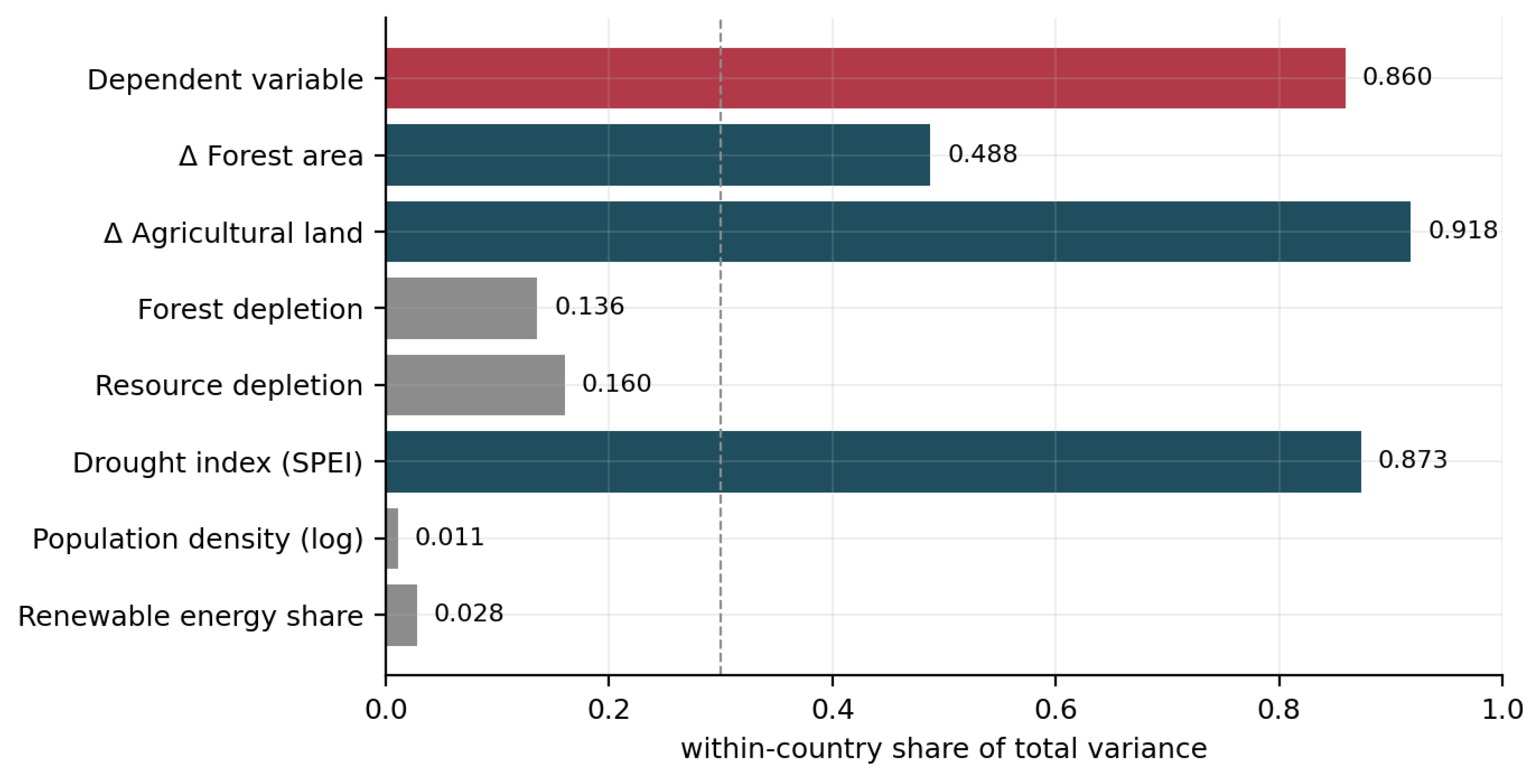
The stability of each coefficient across the six estimators is summarised in the following figure, which partitions the block into three groups: coefficients whose confidence intervals exclude zero in every specification, coefficients whose significance depends on the dimension of variance exploited, and the single coefficient whose interval lies on opposite sides of zero in the two dimensions.
Figure A2.
Point estimates and 95 per cent confidence intervals by estimator. Dark markers denote significance at the 5 per cent level.
Figure A2.
Point estimates and 95 per cent confidence intervals by estimator. Dark markers denote significance at the 5 per cent level.
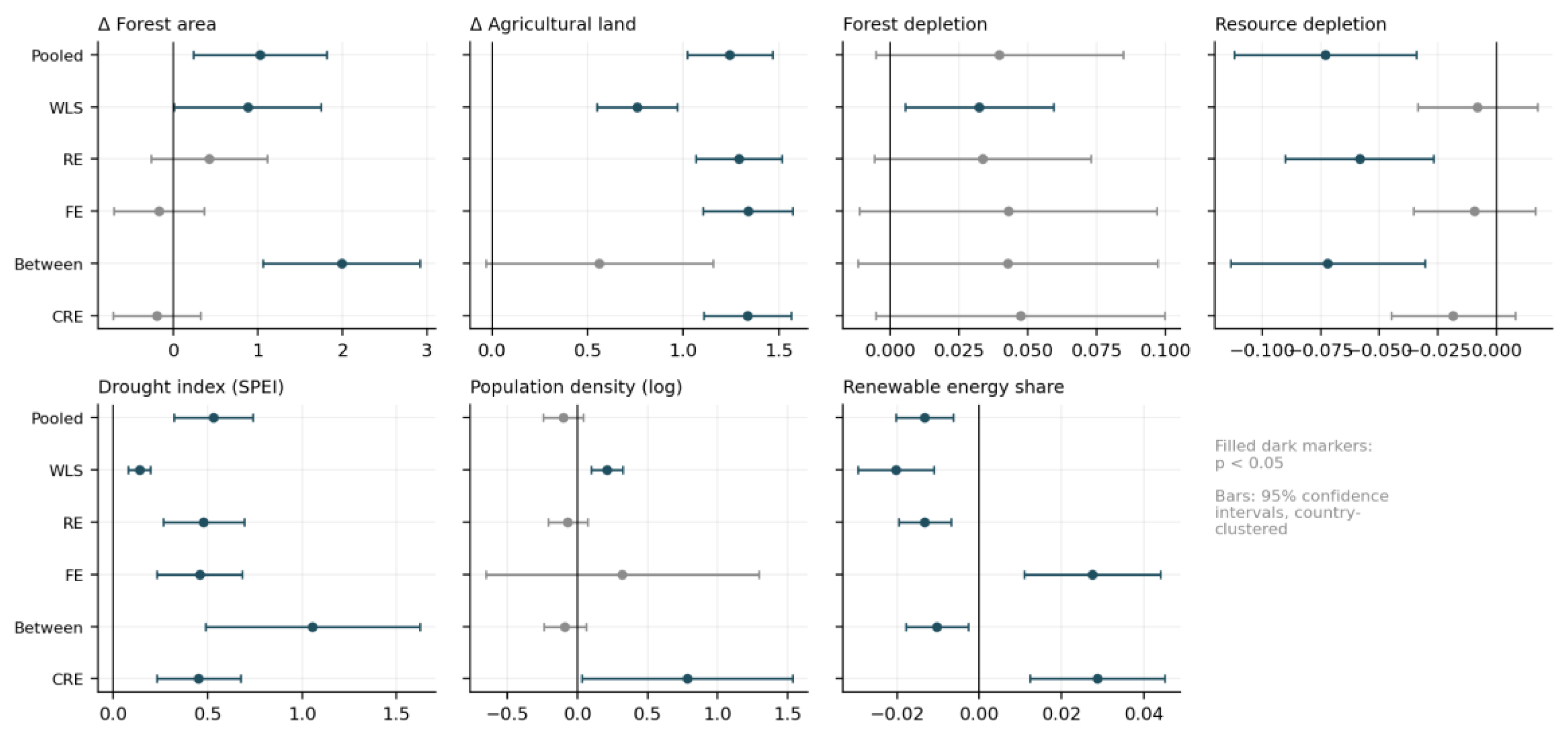
The concern that the land-use coefficients reflect the construction of the accounts rather than an economic relationship is addressed by decomposing the dependent variable into its components and re-estimating on subsets of them.
Figure A3.
Left panel: mean composition of renewable natural capital by component. Right panel: fixed-effects coefficients estimated on total renewable natural capital and on the same aggregate excluding agricultural land, with 95 per cent confidence intervals.
Figure A3.
Left panel: mean composition of renewable natural capital by component. Right panel: fixed-effects coefficients estimated on total renewable natural capital and on the same aggregate excluding agricultural land, with 95 per cent confidence intervals.
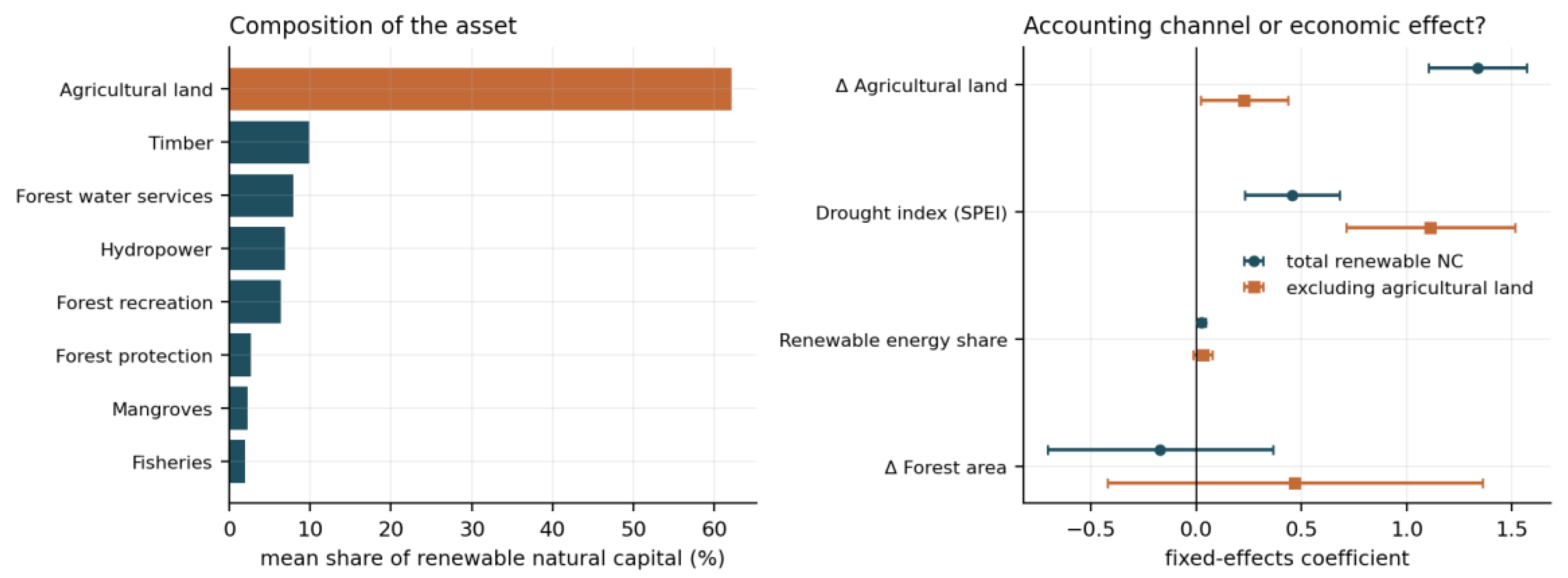
Agricultural land accounts for 62.1 per cent of renewable natural capital on average, followed by timber at 9.9 per cent, forest water services at 7.9 per cent, hydropower at 6.9 per cent and forest recreation at 6.4 per cent, with protective forest services, mangroves and fisheries together contributing less than seven per cent. Excluding agricultural land from the dependent variable reduces the coefficient on the change in agricultural land from 1.338 to 0.229 and raises the drought coefficient from 0.457 to 1.113. Restricting the dependent variable to the four forest components instead returns a coefficient on the change in forest area of 1.109, significant at the five per cent level, against a coefficient indistinguishable from zero on the total aggregate. Each land-use variable therefore acts principally on the component of the asset to which it belongs, as the accounting interpretation predicts, while the drought index acts on the components least insulated by agricultural support policies.
Section 4 rests on the comparison between the within coefficients and the group-mean terms of the Mundlak specification, reported in full below. A group-mean term differing significantly from zero indicates that the between and within relationships are not the same relationship.
Table A2.
Mundlak correlated random effects specification.
| Variable | Within term | Group-mean term | p-value on the group mean |
| Δ Forest area | −0.1985 | 2.2016 | 0.0001 |
| Δ Agricultural land | 1.3371 | −0.7933 | 0.0145 |
| Net forest depletion | 0.0473 | −0.0064 | 0.8587 |
| Natural resources depletion | −0.0186 | −0.0538 | 0.0211 |
| Drought index (SPEI) | 0.4524 | 0.6204 | 0.0370 |
| Population density (log) | 0.7827 | −0.8777 | 0.0260 |
| Renewable energy share | 0.0287 | −0.0385 | 0.0000 |
Note. Joint Wald test on the seven group means: 70.998, p < 0.001.
Five of the seven group-mean terms are significant at the five per cent level, which is a strong statement about the design of the study: for most of the environmental block the cross-country and the year-to-year relationships differ. The renewable energy share is the clearest case, with terms of opposite sign; the change in forest area is the second, with a between term of 2.20 against a within term indistinguishable from zero. The remaining specification tests are collected in the following table.
Table A3.
Specification and diagnostic tests, two-way fixed-effects specification, N = 3,611.
| Test | Statistic | p-value | Implication |
| F test on country effects | 3.814 | < 0.001 | Country effects jointly significant; pooling rejected |
| Hausman, FE against RE | 76.409 | < 0.001 | Effects correlated with regressors; FE preferred |
| Breusch–Pagan LM | 334.139 | < 0.001 | Unobserved heterogeneity present; pooled OLS inefficient |
| Mundlak joint test | 70.998 | < 0.001 | CRE preferred to conventional RE |
| Wooldridge test for AR(1) | −0.169 | 0.091 | No serial correlation at the 5 per cent level |
| Pesaran CD | 3.155 | 0.002 | Cross-sectional dependence, mean absolute correlation 0.181 |
Two of these require a response. The negative and insignificant Wooldridge statistic is consistent with the absence of persistence documented in A.4 and means no correction for serial correlation is required. The Pesaran test rejects cross-sectional independence, although the mean absolute residual correlation of 0.181 is moderate and the year effects already absorb the common component; re-estimating with Driscoll–Kraay standard errors leaves the change in agricultural land, the drought index and the renewable energy share significant at the five per cent level, the last of the three moving from a p-value of 0.001 to 0.040.
Estimating the equation with the lagged dependent variable, by least squares with dummy variables and both sets of effects retained, returns an autoregressive coefficient of −0.154 with a standard error of 0.088. The Anderson–Hsiao instrumental variable estimator applied to the first-differenced equation, using the second lag of the dependent variable as instrument, returns −0.099 with a standard error of 0.071 and a first-stage F statistic of 168.3. Both are negative rather than positive, and the least squares dummy variable estimate is biased downward by an amount of order 1/T in a panel of twenty-five periods, so the true value is likely closer to zero than to −0.15.
The substantive conclusion is that the growth of renewable natural capital per capita carries no inertia: the raw first-order autocorrelation of the dependent variable is 0.01. A country that lost natural capital rapidly last year is not thereby more likely to lose it rapidly this year, once permanent characteristics and the common year effect are removed. There is consequently no meaningful distinction between short-run and long-run multipliers, which is why the coefficients in the dynamic specification are almost identical to their static counterparts, at 1.339 for the change in agricultural land, 0.472 for the drought index and 0.023 for the renewable energy share.
None of the results is presented as causal. The drought index is the identification anchor of the equation, being constructed from precipitation and evapotranspiration and not plausibly influenced by national wealth accounts. At the opposite extreme, the change in agricultural land is not a candidate for instrumentation, since the difficulty there is an accounting relationship rather than simultaneity and an instrument would deliver a precisely estimated coefficient on an identity; population density is equally unsuitable, its within variation being roughly one per cent of the total.
Two regressors raise a genuine simultaneity concern and were tested. The renewable energy share may respond to the abundance of hydropower and biomass, themselves components of the dependent variable, and resource depletion responds to world commodity prices which also move the valuation of the asset. For each, a shift-share instrument was constructed by interacting initial country exposure, measured in the first observed year, with an annual global shock computed as the leave-one-out mean across all other countries and normalised by the country mean; the equation was then re-estimated by two-stage least squares after removing country and year effects, so that the identifying variation is the differential response of countries with different initial exposure to a common annual movement.
Table A4.
Shift-share instrumental variable estimates.
| Endogenous regressor | First stage | First-stage F | FE estimate | 2SLS estimate | Wu–Hausman p |
| Renewable energy share | 1.2938 (0.2458) | 27.72 | 0.0274 (0.0083) | 0.0388 (0.0389) | 0.757 |
| Natural resources depletion | 0.4634 (0.1099) | 17.79 | −0.0095 (0.0130) | −0.0999 (0.0867) | 0.094 |
Note. Country-clustered standard errors in parentheses. Each row instruments one regressor while retaining the remaining six as exogenous controls.
Instrumentation neither rescues nor overturns any finding. For the renewable energy share the instrumented coefficient has the same sign and a comparable magnitude to the fixed-effects estimate, with a standard error almost five times wider that leaves it short of significance, and the Wu–Hausman test does not reject exogeneity; this matters because that coefficient carries the argument about the two dimensions of variation. For resource depletion the instrumented coefficient remains insignificant. Both first stages clear the conventional relevance threshold of ten without reaching the more demanding thresholds now recommended for weak-instrument-robust inference, which is why these estimates are reported as a check rather than as a preferred specification. The exclusion restriction is stronger for the renewable energy share than for resource depletion, since a commodity price movement interacted with initial resource exposure may affect the valuation of agricultural land directly and not only through the extraction channel.
Significance was re-assessed by a wild cluster bootstrap-t with Rademacher weights and the null imposed, resampling at the country level over 1,999 replications, with the restricted model re-estimated separately for each coefficient tested.
Table A5.
Wild cluster bootstrap-t p-values, 1,999 replications.
| Variable | FE coefficient | Cluster-robust p | Bootstrap p | Survives Bonferroni |
| Δ Agricultural land | 1.3377 | 0.0000 | 0.0005 | Yes |
| Drought index (SPEI) | 0.4571 | 0.0001 | 0.0005 | Yes |
| Renewable energy share | 0.0274 | 0.0012 | 0.0010 | Yes |
| Net forest depletion | 0.0429 | 0.1198 | 0.1300 | No |
| Natural resources depletion | −0.0095 | 0.4741 | 0.4490 | No |
| Population density (log) | 0.3195 | 0.5208 | 0.5320 | No |
| Δ Forest area | −0.1706 | 0.5314 | 0.7570 | No |
Note. The Bonferroni threshold over seven coefficients is 0.00714.
The bootstrap p-values track the cluster-robust ones closely, as expected with 149 clusters, and the ordering of coefficients by strength of evidence is unchanged. Eight further specifications were then estimated, each modifying one element of the baseline while leaving the rest unchanged; only the three coefficients that survived the bootstrap are reported, the remaining four being insignificant throughout.
Table A6.
Alternative specifications.
| Specification | Δ Agricultural land | Drought index | Renewable energy share | N |
| Baseline, two-way FE | 1.3377*** | 0.4571*** | 0.0274*** | 3,611 |
| Adding log GDP per capita | 1.3379*** | 0.4567*** | 0.0288*** | 3,611 |
| Excluding agricultural land from the dependent variable | 0.2286** | 1.1129*** | 0.0317 | 3,611 |
| Dependent variable winsorised at 1/99 | 1.0223*** | 0.3834*** | 0.0232*** | 3,611 |
| Excluding 2020 | 1.3720*** | 0.4323*** | 0.0302*** | 3,464 |
| Driscoll–Kraay standard errors | 1.3377*** | 0.4571*** | 0.0274** | 3,611 |
| One-way FE, no year effects | 1.3371*** | 0.4524*** | 0.0287*** | 3,611 |
| High-income half of the sample | 1.5538*** | 0.6650*** | −0.0109 | 1,750 |
| Low-income half of the sample | 1.0777*** | 0.2473*** | 0.0255** | 1,861 |
Note. Significance: *** p<0.01; ** p<0.05; * p<0.10. Country-clustered standard errors except where indicated.
Adding income leaves the three coefficients unchanged and returns an income coefficient of 0.090 with a p-value of 0.706, so the results are not a restatement of development. Winsorising confirms that the estimates are not driven by the tails, and excluding 2020 that the pandemic year is not responsible for them. Dropping the year effects raises the population density coefficient to 0.783 with a p-value of 0.041, which is precisely the spurious significance that the variance decomposition anticipates and which disappears once common shocks are absorbed. The income split is the most informative of the eight: the drought coefficient is substantially larger in the richer half, at 0.665 against 0.247, while the renewable energy coefficient is positive and significant only in the poorer half, as the traditional biomass interpretation predicts.
Appendix B. The E–Environment Clustering
The three criteria used to fix k are displayed below over the range from two to ten, all computed on the k-means solution so that the comparison is internally consistent.
Figure A4.
Selection of the number of clusters. Left: average silhouette width. Centre: explained variance. Right: marginal reduction in within-cluster deviance. The dashed line and the highlighted bar mark the retained solution.
Figure A4.
Selection of the number of clusters. Left: average silhouette width. Centre: explained variance. Right: marginal reduction in within-cluster deviance. The dashed line and the highlighted bar mark the retained solution.
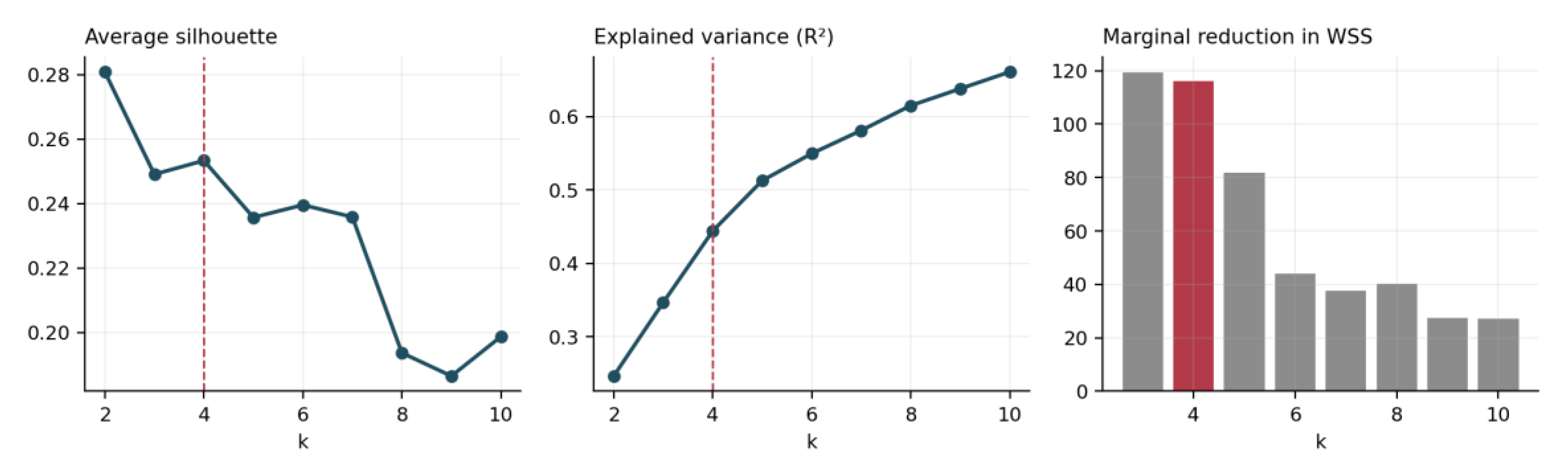
Table A7.
Selection statistics for the k-means solution, k from 2 to 10, 149 countries.
| k | R2 | Silhouette | Calinski–Harabasz | AIC | BIC | Within deviance | Marginal reduction |
| 2 | 0.247 | 0.281 | 48.12 | −301.5 | −247.5 | 898.0 | — |
| 3 | 0.347 | 0.249 | 38.73 | −453.4 | −372.3 | 778.8 | 119.3 |
| 4 | 0.444 | 0.253 | 38.62 | −628.0 | −519.9 | 662.6 | 116.2 |
| 5 | 0.513 | 0.236 | 37.89 | −767.2 | −632.0 | 580.7 | 81.8 |
| 6 | 0.550 | 0.240 | 34.91 | −842.9 | −680.7 | 536.8 | 43.9 |
| 7 | 0.581 | 0.236 | 32.84 | −911.4 | −722.1 | 499.3 | 37.6 |
| 8 | 0.615 | 0.194 | 32.17 | −993.7 | −777.4 | 459.0 | 40.3 |
| 9 | 0.638 | 0.186 | 30.84 | −1049.1 | −805.8 | 431.5 | 27.4 |
| 10 | 0.661 | 0.199 | 30.09 | −1108.9 | −838.5 | 404.3 | 27.3 |
The information criteria decline monotonically over the whole range and therefore provide no interior optimum, which is the expected behaviour when the likelihood is approximated from the within-cluster deviance and the penalty grows only linearly in k. They are reported for completeness and were not used to select the solution. The Calinski–Harabasz statistic falls monotonically from k = 2 and likewise offers no interior maximum. The decision therefore rests on the elbow in the marginal reduction of deviance, which is sharp between k = 4 and k = 5, and on the local maximum of the silhouette at k = 4.
The mean rank reported in the body of the section conceals substantial variation across indices, and the two panels below show both the aggregate and its components.
Figure A5.
Left: mean rank across the eleven internal validity indices, lower being better. Right: four selected indices, min–max normalised across the six algorithms.
Figure A5.
Left: mean rank across the eleven internal validity indices, lower being better. Right: four selected indices, min–max normalised across the six algorithms.
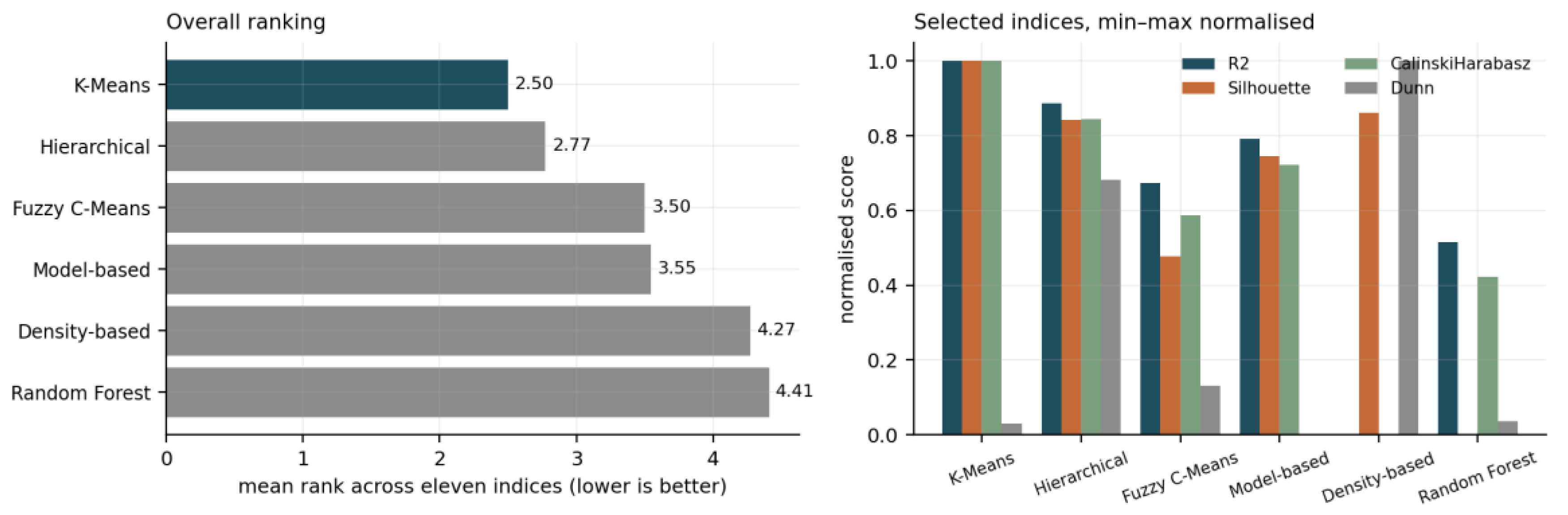
Density-based clustering was tuned by searching the neighbourhood radius over the interval from 0.9 to 3.5 in steps of 0.05, retaining the value maximising the silhouette subject to producing at least three clusters and leaving no more than 35 per cent of observations unassigned. The retained configuration has a radius of 2.15 and a minimum neighbourhood size of four, yields four clusters and classifies nineteen countries as noise. The indices reported for this algorithm are computed on the 130 assigned observations, which is why its explained variance is not directly comparable with the others and why its ranking should be read with that qualification.
The fuzzy c-means solution was estimated with a fuzzifier of two and three hundred iterations, and the reported partition assigns each country to the cluster of maximum membership. Its distinguishing feature in the comparison is the most balanced size distribution, with the highest entropy at 1.309 and the lowest Herfindahl index at 0.289, which is a consequence of the soft assignment rule rather than of a better recovery of structure; on the indices that measure compactness and separation it ranks below both k-means and hierarchical clustering.
Projecting the standardised data onto the first two principal components, which together account for 52.2 per cent of the total variance, gives a visual account of what separates the four groups.
Figure A6.
The four clusters in the plane of the first two principal components, with the loadings of the eight variables shown as arrows.
Figure A6.
The four clusters in the plane of the first two principal components, with the loadings of the eight variables shown as arrows.
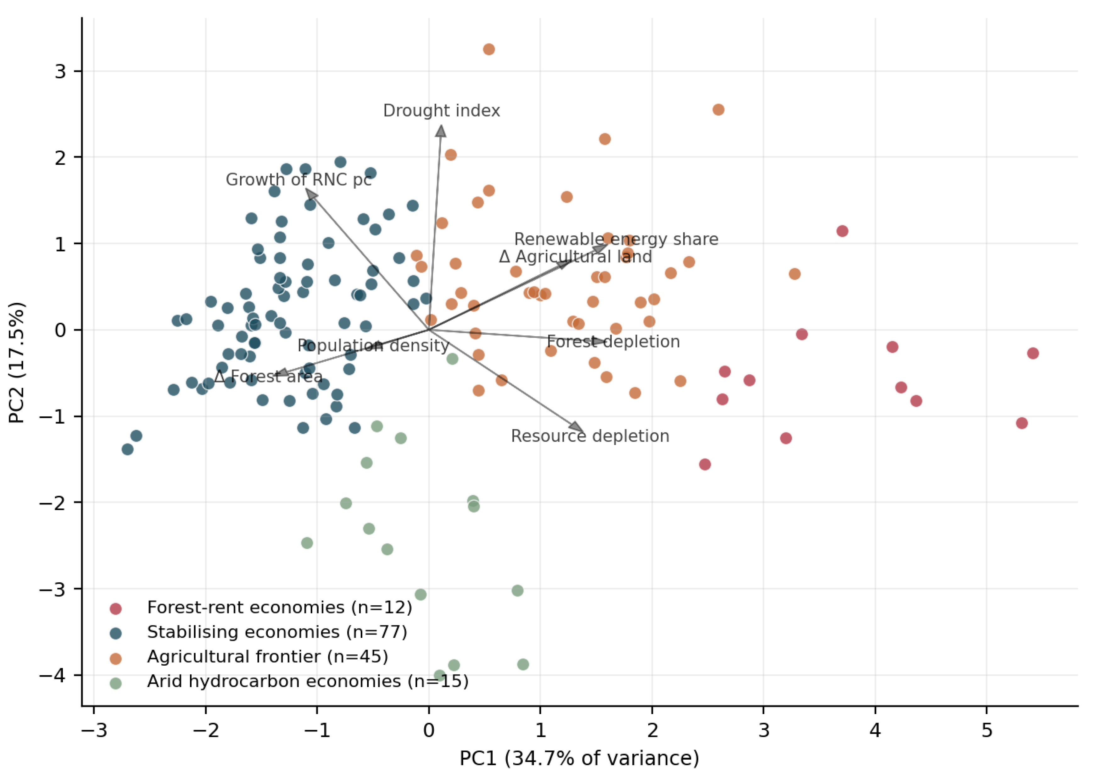
The first component, at 34.7 per cent of variance, is an axis of extraction: it loads positively on the renewable energy share, at 0.466, on forest depletion, at 0.457, on resource depletion, at 0.400, and on the expansion of agricultural land, at 0.365, and negatively on the growth of renewable natural capital, at −0.321, and on the change in forest area, at −0.398. Movement to the right along this axis is movement from stabilised land use towards active depletion, and it orders three of the four clusters. The second component, at 17.5 per cent, is dominated by the drought index, at 0.700, and by the growth of the dependent variable, at 0.478. It is what separates the arid hydrocarbon economies, which sit low on this axis while occupying the same region of the first axis as the stabilising economies, from every other group. The classification is therefore genuinely two-dimensional: a single index of environmental pressure would collapse the fourth cluster into the first.
Figure A7.
Left: distribution of silhouette widths within each cluster. Right: mean growth of renewable natural capital per capita by cluster, with standard errors.
Figure A7.
Left: distribution of silhouette widths within each cluster. Right: mean growth of renewable natural capital per capita by cluster, with standard errors.
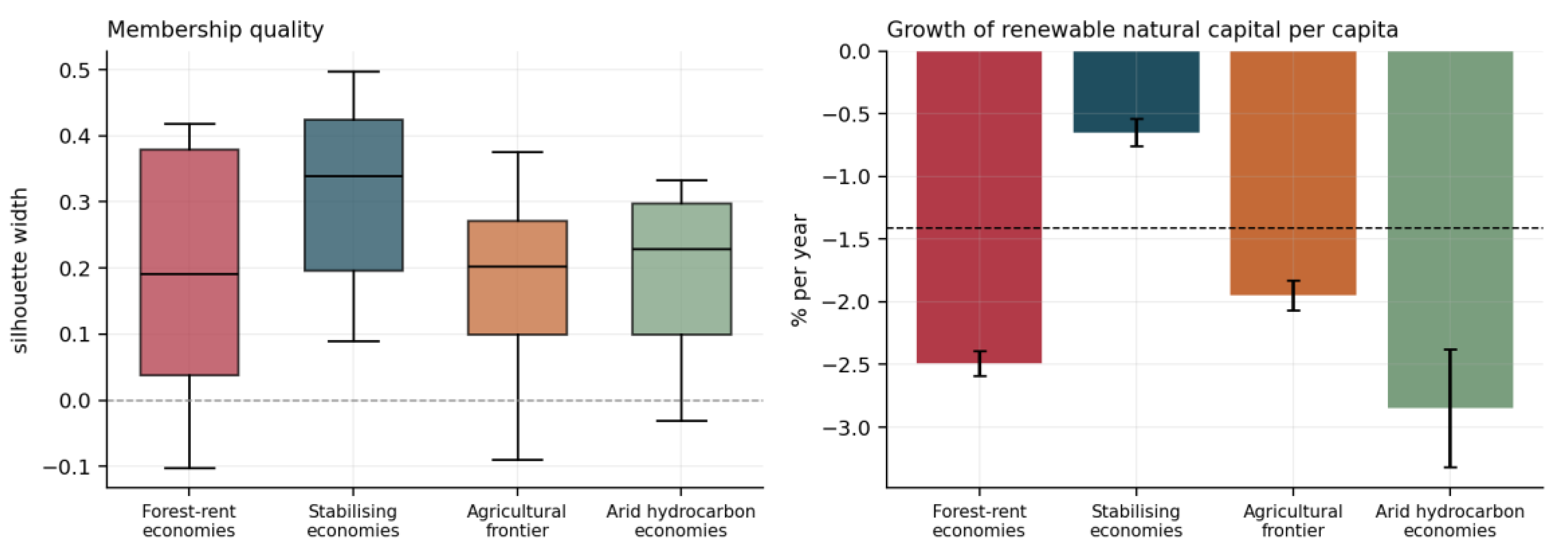
The stabilising economies form the most cohesive group, with a mean silhouette of 0.317, while the other three lie between 0.180 and 0.199. Eight countries in total have a negative silhouette width, indicating that they are closer on average to a neighbouring group than to their own; all eight lie on the boundary between the stabilising and the agricultural frontier clusters, which is where the classification is least sharp.
Table A8.
Cluster profiles in the original units of measurement.
| Cluster | n | Growth of RNC pc (%) | Resource depletion | Forest depletion | Renewable energy | Drought index | Representative members |
| Stabilising economies | 77 | −0.65 | 1.06 | 0.13 | 21.6 | −0.17 | France, Germany, Japan, Poland, Romania, Türkiye |
| Agricultural frontier | 45 | −1.95 | 3.85 | 2.01 | 60.7 | −0.11 | Tanzania, Mozambique, Côte d’Ivoire, Cambodia, Nicaragua, Nigeria |
| Forest-rent economies | 12 | −2.49 | 19.89 | 12.19 | 83.9 | −0.20 | DR Congo, Liberia, Ethiopia, Gabon, Angola, Chad |
| Arid hydrocarbon economies | 15 | −2.85 | 10.41 | 0.11 | 5.1 | −0.84 | Saudi Arabia, UAE, Kuwait, Iraq, Egypt, Kazakhstan |
Note. Depletion variables are percentages of gross national income, the renewable energy share a percentage of final consumption, the drought index a standardised score.
The table makes the internal logic of the taxonomy explicit. The three groups losing natural capital fastest do so for different reasons: the forest-rent economies through the extraction of timber and minerals, at a combined 32 per cent of national income; the agricultural frontier economies through the conversion of forest into cropland; and the arid hydrocarbon economies through a combination of subsoil extraction and a biophysical environment in which the renewable asset base is thin to begin with. Only the first group is losing natural capital in a way that a resource-rent taxation policy could plausibly address, which is the principal policy implication of the classification and the reason a single composite ranking of environmental performance would be misleading here.
Appendix C. The E–Environment Machine Learning Validation
The right-hand panel is the substantive one. The ordering of the models by in-sample fit is almost the reverse of their ordering by out-of-sample fit, which is the signature of overfitting in a panel with strong unobserved heterogeneity: the flexible learners memorise features of the training observations that do not generalise. Grouping the folds by country was adopted as a precaution against a second and more subtle version of the same problem, in which a learner recognises an individual economy from the joint distribution of its residualised regressors and reproduces its average outcome. As a check, the comparison was repeated with conventional random folds, which returns 0.1865 for the linear model, 0.1442 for the random forest and 0.1177 for boosting. The ordering is unchanged and the margin in favour of the linear specification is marginally wider, so the conclusion of this module does not depend on the folding strategy. The grouped design is retained because it is the more conservative of the two, and because in panels with fewer periods the distinction would matter considerably more than it does here.
Figure A8.
Left: cross-validated coefficient of determination by model, folds grouped by country. Right: in-sample against cross-validated performance for the same six models.
Figure A8.
Left: cross-validated coefficient of determination by model, folds grouped by country. Right: in-sample against cross-validated performance for the same six models.
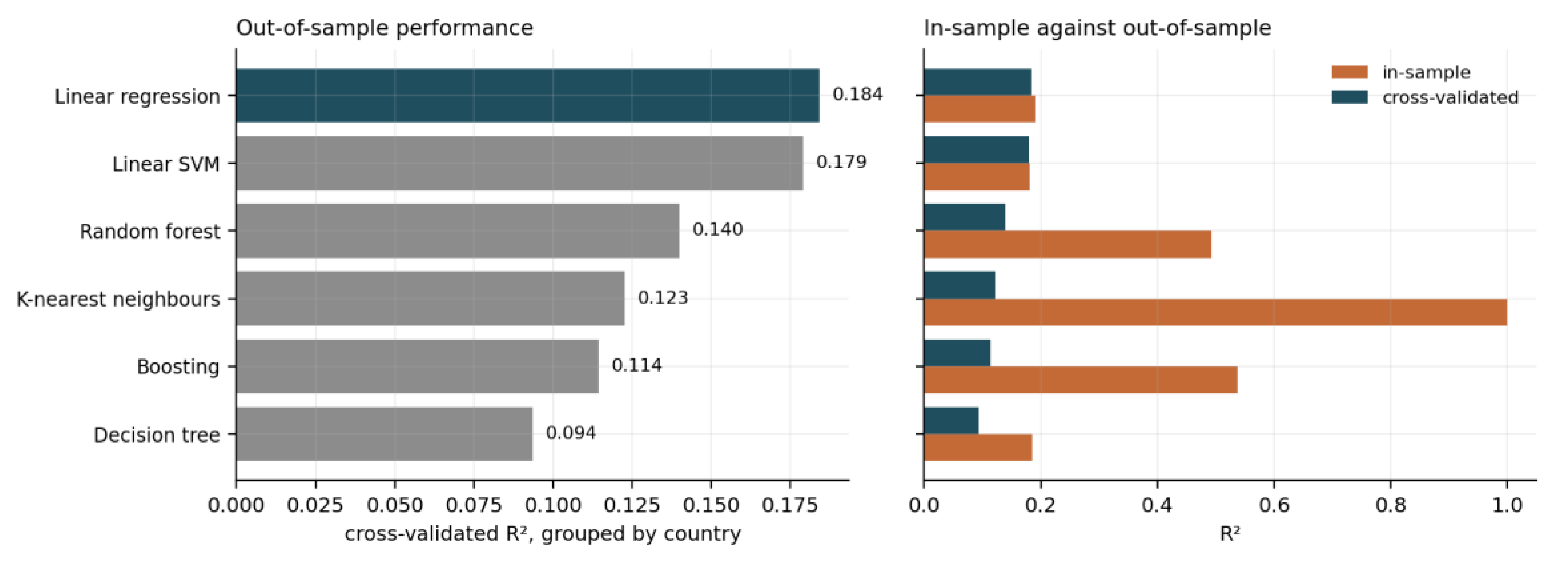
The hyperparameters were fixed rather than tuned, at values conventional for samples of this size: twenty-five neighbours for k-nearest neighbours, depth six and a minimum leaf size of thirty for the single tree, six hundred trees with a minimum leaf size of five and sixty per cent of features sampled at each split for the random forest, and six hundred stages with a learning rate of 0.03 and eighty per cent subsampling for boosting. Tuning within the cross-validation loop was not attempted, and this is a limitation that should be stated plainly: a systematically optimised ensemble might narrow the gap reported in Table 7. It is unlikely to close it, since the source of the linear model’s advantage is visible in the partial dependence functions, which are close to straight lines over the region where the data are dense, and no amount of tuning makes a flexible learner match a linear one on a relationship that is in fact linear. The claim defended here is the weaker and safer one: on conventional settings, flexibility does not help.
Table A9.
Random forest attribution against the fixed-effects estimates.
| Regressor | Permutation share | Mean abs. SHAP | SHAP share | SHAP direction | FE coefficient | Bootstrap p | Signs agree |
| Δ Agricultural land | 0.445 | 0.647 | 0.452 | +0.951 | 1.3377 | 0.0005 | Yes |
| Drought index (SPEI) | 0.193 | 0.332 | 0.232 | +0.847 | 0.4571 | 0.0005 | Yes |
| Renewable energy share | 0.096 | 0.115 | 0.081 | +0.511 | 0.0274 | 0.0010 | Yes |
| Δ Forest area | 0.074 | 0.102 | 0.071 | +0.391 | −0.1706 | 0.7570 | No |
| Population density (log) | 0.075 | 0.096 | 0.067 | −0.031 | 0.3195 | 0.5320 | No |
| Net forest depletion | 0.059 | 0.072 | 0.051 | +0.112 | 0.0429 | 0.1300 | Yes |
| Natural resources depletion | 0.059 | 0.068 | 0.047 | +0.131 | −0.0095 | 0.4490 | No |
Note. Permutation importance uses twenty repetitions and the mean squared error as the scoring function. SHAP direction is the correlation between the value of the regressor and its SHAP contribution. Bootstrap p-values are those of Table A5.
The two attribution methods agree closely with each other, which is not automatic: permutation importance measures the loss in accuracy when a variable is randomised, and is therefore sensitive to correlation among regressors, while SHAP values decompose each individual prediction and are additive by construction. Their agreement here follows from the low collinearity documented in Appendix A.1. The population density row is the only one where the two diverge in interpretation: permutation importance assigns it 7.5 per cent, more than forest or resource depletion receive, while its SHAP direction is essentially zero at −0.031, indicating that the forest uses the variable to make local adjustments without any systematic directional effect. This is consistent with the econometric finding that the variable has almost no within-country variation to speak of.
Figure A9.
SHAP contributions of the three regressors significant in the econometric model, plotted against the value of the regressor. Each point is one country-year observation.
Figure A9.
SHAP contributions of the three regressors significant in the econometric model, plotted against the value of the regressor. Each point is one country-year observation.
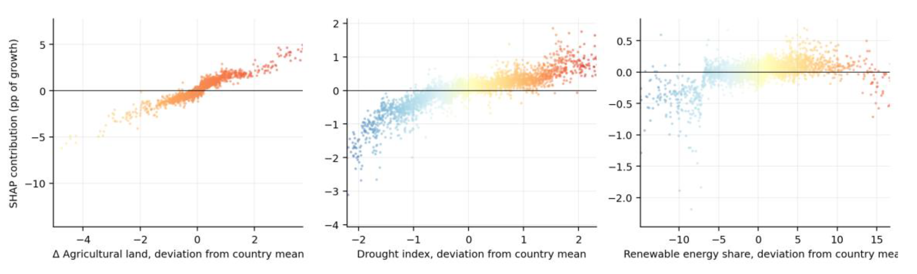
The three panels display the near-linear relationship between a regressor and its contribution that the partial dependence functions summarise. The dispersion around the central relationship measures the extent to which the contribution of a variable depends on the values of the others, and it is visibly narrow for the change in agricultural land, wider for the drought index and widest for the renewable energy share, which is the same ordering as the linearity of the partial dependence curves.
Figure A10.
Partial dependence functions from the random forest, with the least-squares line through each curve shown as a dashed line.
Figure A10.
Partial dependence functions from the random forest, with the least-squares line through each curve shown as a dashed line.
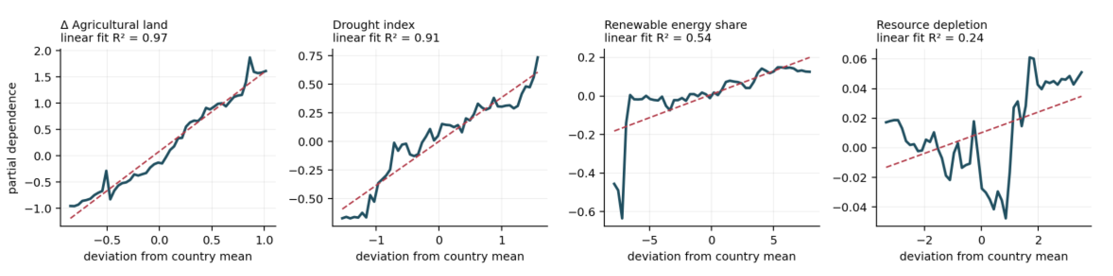
Table A10.
Out-of-sample performance of extended linear specifications, ten-fold cross-validation grouped by country.
Table A10.
Out-of-sample performance of extended linear specifications, ten-fold cross-validation grouped by country.
| Specification | Cross-validated R2 | Change from baseline |
| Linear, seven regressors | 0.1842 | — |
| Adding twenty-one interactions | 0.1794 | −0.0048 |
| Adding seven squared terms | 0.1843 | +0.0001 |
| Adding both | 0.1758 | −0.0084 |
The table is the formal counterpart of the partial dependence curves. Interactions reduce performance, which is what happens when twenty-one additional parameters are estimated on variation that does not support them, and squared terms leave it unchanged to four decimal places. The apparent curvature of the renewable energy function, with a linear fit of 0.540, is therefore not strong enough to improve prediction when imposed as a quadratic; a threshold specification, in which the effect is zero below a cutoff and constant above it, would be the natural way to test it, and is left for future work since it would require a data-driven choice of cutoff that this sample is not large enough to estimate reliably. The honest statement is that the linear form is adequate for the three relationships the paper claims, and that one of them may be a threshold rather than a slope.
Appendix D. The S–Social Equation
The final column records the practical consequence of the variance decomposition. Three of the seven regressors carry less than five per cent of their variation within countries, so their fixed-effects coefficients are estimated on very little information and their cross-sectional estimates should be given interpretive priority; two carry almost all of their variation within countries and are identified by the fixed-effects estimator alone. Only population growth and the share of women in parliament contribute meaningfully in both dimensions. The fertility rate is the awkward case: it is between-identified by this criterion, at 4.5 per cent, yet the coefficient that survives every test in this section is its fixed-effects estimate, which is more than three times the pooled estimate. The explanation is that the within variation, though small as a share, is large in absolute terms over twenty-four years, since fertility declines substantially in most developing economies across the period.
Table A11.
Descriptive statistics and variance decomposition, 151 countries, 1997–2020, N = 3,293.
| Variable | Mean | SD | Within share | Role in the equation |
| Growth of renewable NC per capita (%) | −1.366 | 3.511 | 0.861 | Dependent variable |
| Growth of total renewable NC (%) | 0.066 | 3.236 | 0.962 | Alternative dependent variable |
| Population growth (%) | 1.432 | 1.571 | 0.286 | Enters the dependent variable by identity |
| Fertility rate (births per woman) | 2.895 | 1.559 | 0.045 | Between-identified |
| Δ Life expectancy (years) | 0.273 | 1.173 | 0.975 | Within-identified |
| Labour force participation (%) | 66.989 | 11.026 | 0.049 | Between-identified |
| Female–male LFP ratio (%) | 71.365 | 18.476 | 0.042 | Between-identified |
| Δ Electricity access (pp) | 0.645 | 2.211 | 0.863 | Within-identified |
| Women in parliament (%) | 18.264 | 11.446 | 0.282 | Mixed |
Figure A11.
Point estimates and 95 per cent confidence intervals by estimator, social block. Dark markers denote significance at the 5 per cent level.
Figure A11.
Point estimates and 95 per cent confidence intervals by estimator, social block. Dark markers denote significance at the 5 per cent level.
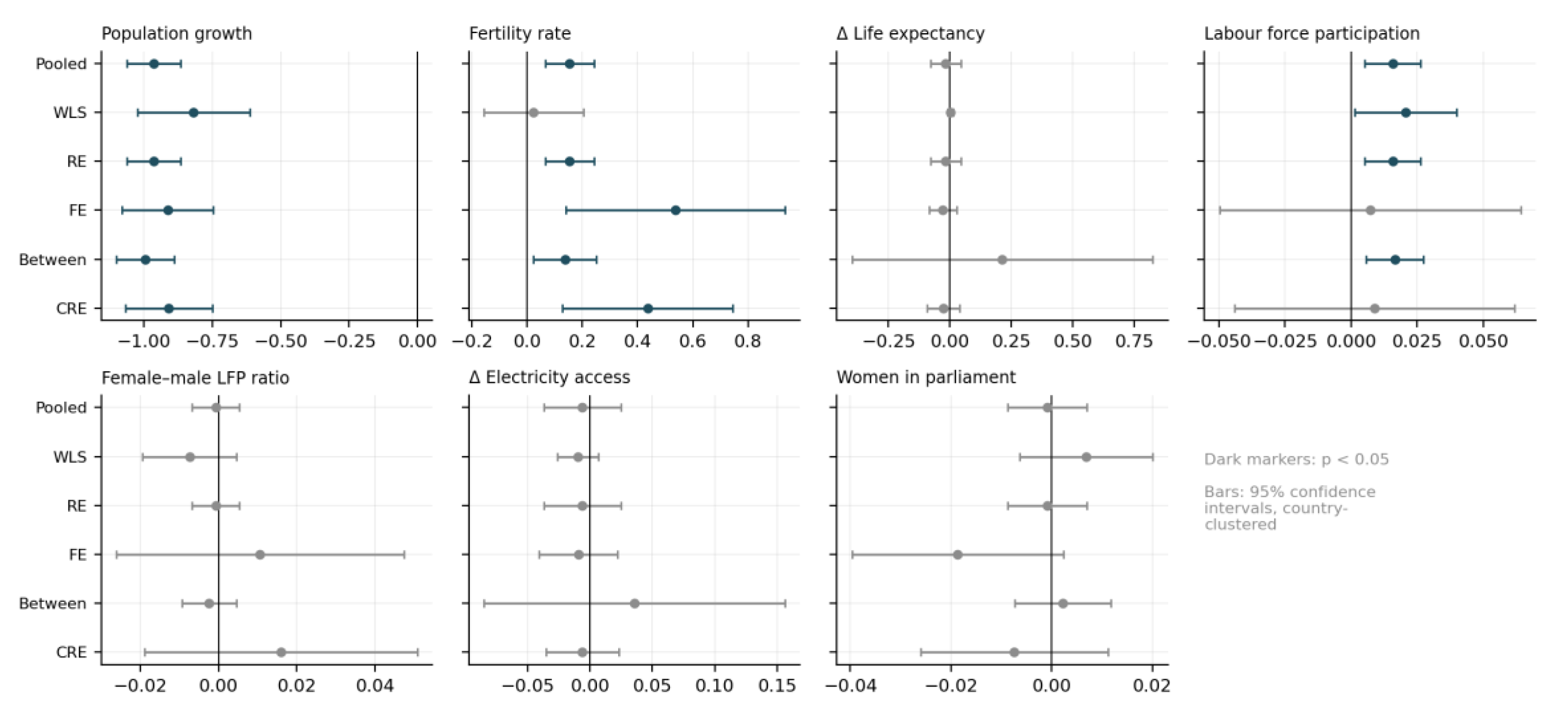
Figure A12.
Left: fixed-effects coefficients estimated on per capita and on total growth of renewable natural capital; the dotted line marks the value implied by the accounting identity. Right: the coefficient on the fertility rate estimated on the total stock and on its two parts.
Figure A12.
Left: fixed-effects coefficients estimated on per capita and on total growth of renewable natural capital; the dotted line marks the value implied by the accounting identity. Right: the coefficient on the fertility rate estimated on the total stock and on its two parts.
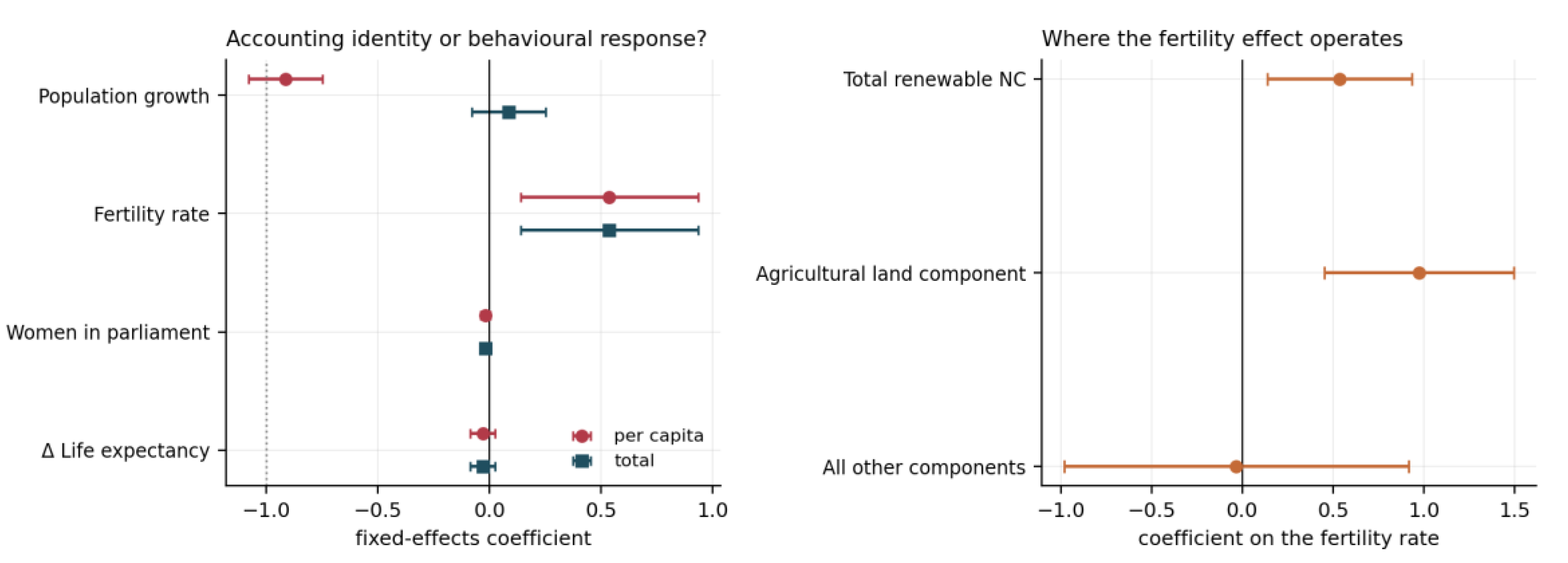
The left panel shows that only population growth moves between the two specifications, and that it moves from a coefficient statistically indistinguishable from the identity value to one indistinguishable from zero. The right panel shows the decomposition of the fertility effect, with a coefficient of 0.975 on the agricultural land component, 0.537 on the total, and −0.033 on the remaining components. Since agricultural land accounts for 62.1 per cent of renewable natural capital on average, the total coefficient is close to what the agricultural coefficient alone implies, and the fertility effect can be described as operating entirely through cultivated land.
Table A12.
The two surviving coefficients under alternative definitions of the dependent variable, two-way fixed effects with country-clustered standard errors.
Table A12.
The two surviving coefficients under alternative definitions of the dependent variable, two-way fixed effects with country-clustered standard errors.
| Dependent variable | Population growth | Fertility rate | N |
| Renewable NC per capita | −0.9132*** | 0.5368*** | 3,293 |
| Total renewable NC | 0.0868 | 0.5368*** | 3,293 |
| Agricultural land component, total | 0.1476 | 0.9747*** | 3,293 |
| All other components, total | −0.1513 | −0.0328 | 3,289 |
| Renewable NC excluding agricultural land, per capita | −1.1513*** | −0.0328 | 3,289 |
The final row is worth noting because it appears to contradict the argument. When agricultural land is removed from the dependent variable but the per capita denominator is retained, population growth returns with a coefficient of −1.151, larger in absolute value than in the baseline. This is not a behavioural effect either: the non-agricultural components are a smaller and more slowly growing base, so the same demographic denominator produces a proportionally larger effect. The row is reported to make explicit that the identity operates on every definition of the dependent variable that is expressed per capita, and that only the change to total quantities removes it.
Table A13.
Specification tests, social block, N = 3,293.
| Test | Statistic | p-value | Comparison with the E block |
| F test on country effects | 0.709 | 0.997 | E block rejects pooling; S block does not |
| Hausman, FE against RE | 6.089 | 0.530 | E block strongly favours FE |
| Breusch–Pagan LM | 8.090 | 0.005 | Significant in both |
| Mundlak joint test | 13.648 | 0.058 | Decisive in E, borderline in S |
| Wooldridge test for AR(1) | −0.214 | 0.004 | Absent in E, present in S |
| Pesaran CD | 4.386 | < 0.001 | Present in both, mean absolute ρ 0.185 |
The contrast with the environmental equation in the final column is the most informative content of this table. The social block leaves so little unexplained cross-country heterogeneity that country effects are jointly insignificant, which is a direct consequence of including a variable that enters the dependent variable by construction. It also introduces serial correlation, which the environmental block did not display, and the negative autoregressive coefficient of the dynamic specification, at −0.201 by least squares with dummy variables and −0.120 by the Anderson–Hsiao estimator with a first-stage F of 101.3, indicates mean reversion in the residual rather than persistence.
Table A14.
Wild cluster bootstrap-t p-values, Rademacher weights with the null imposed, 1,999 replications.
Table A14.
Wild cluster bootstrap-t p-values, Rademacher weights with the null imposed, 1,999 replications.
| Variable | FE coefficient | Cluster-robust p | Bootstrap p | Survives Bonferroni |
| Population growth | −0.9132 | 0.0000 | 0.0005 | Yes |
| Fertility rate | 0.5368 | 0.0081 | 0.0050 | Yes |
| Women in parliament | −0.0187 | 0.0817 | 0.0825 | No |
| Δ Life expectancy | −0.0283 | 0.3195 | 0.1905 | No |
| Δ Electricity access | −0.0092 | 0.5684 | 0.5650 | No |
| Female–male LFP ratio | 0.0106 | 0.5713 | 0.5520 | No |
| Labour force participation | 0.0072 | 0.8051 | 0.8080 | No |
Note. The Bonferroni threshold over seven coefficients is 0.00714.
Two coefficients survive, and one of them is an identity, so the substantive content of the social block reduces to the fertility result. The instrumental variable estimates below were computed on the three regressors for which simultaneity is a plausible concern, using the shift-share design described in Appendix A.5.
Table A15.
Shift-share instrumental variable estimates, social block.
| Endogenous regressor | First-stage F | FE estimate | 2SLS estimate | Wu–Hausman p |
| Fertility rate | 155.61 | 0.5368 (0.2033) | 0.5398 (0.2714) | 0.991 |
| Female–male LFP ratio | 34.99 | 0.0106 (0.0188) | 0.0733 (0.0474) | 0.205 |
| Population growth | 6.16 | −0.9132 (0.0850) | −1.7346 (0.4088) | 0.001 |
Note. Standard errors clustered by country in parentheses.
The first row is the useful one. The instrument is strong by any threshold, the instrumented and uninstrumented estimates are almost identical, and the endogeneity test is as far from rejection as it is possible to be, so the fertility coefficient is not driven by reverse causation from land abundance to fertility. The third row should not be read as evidence of anything: the first-stage F of 6.2 is below the conventional relevance threshold, and the divergence between the two estimates reflects instrument weakness rather than bias in the fixed-effects estimate, which in any case measures an accounting relationship whose value is known a priori.
Appendix E. The S–Social Clustering
Figure A13.
Selection of the number of clusters, social block. Left: average silhouette width. Centre: explained variance. Right: marginal reduction in within-cluster deviance.
Figure A13.
Selection of the number of clusters, social block. Left: average silhouette width. Centre: explained variance. Right: marginal reduction in within-cluster deviance.
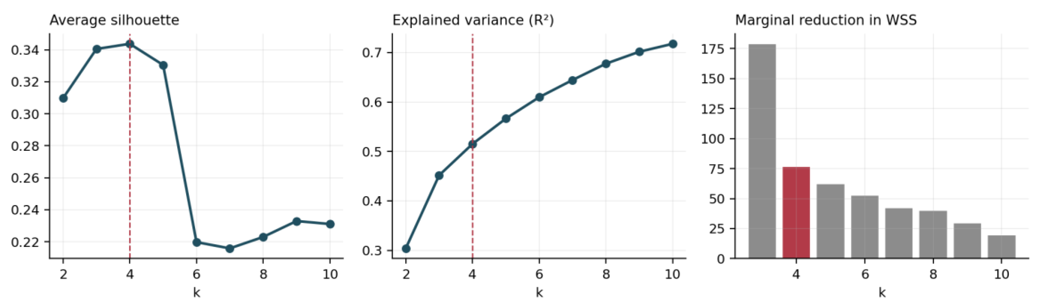
Table A16.
Selection statistics for the k-means solution on the social block, k from 2 to 10, 151 countries.
Table A16.
Selection statistics for the k-means solution on the social block, k from 2 to 10, 151 countries.
| k | R2 | Silhouette | Calinski–Harabasz | AIC | BIC | Within deviance | Marginal reduction |
| 2 | 0.304 | 0.310 | 65.05 | −401.6 | −347.3 | 840.9 | — |
| 3 | 0.452 | 0.340 | 60.95 | −671.8 | −590.4 | 662.4 | 178.5 |
| 4 | 0.515 | 0.344 | 52.04 | −802.2 | −693.6 | 585.8 | 76.5 |
| 5 | 0.566 | 0.330 | 47.66 | −919.2 | −783.4 | 523.9 | 61.9 |
| 6 | 0.610 | 0.220 | 45.28 | −1028.1 | −865.2 | 471.6 | 52.3 |
| 7 | 0.644 | 0.216 | 43.47 | −1122.7 | −932.6 | 429.7 | 42.0 |
| 8 | 0.677 | 0.223 | 42.89 | −1222.5 | −1005.2 | 389.8 | 39.9 |
| 9 | 0.701 | 0.233 | 41.71 | −1298.3 | −1053.9 | 360.6 | 29.1 |
| 10 | 0.718 | 0.231 | 39.79 | −1347.0 | −1075.5 | 341.2 | 19.4 |
The silhouette maximum at k = 4 is genuine rather than marginal, since the fall to k = 6 is from 0.344 to 0.220. As in the environmental block the information criteria decline monotonically and offer no interior optimum, and the Calinski–Harabasz statistic falls from k = 2; neither was used in the decision, which rests on the silhouette and is corroborated by the deviance elbow.
Figure A14.
Left: mean rank across the eleven internal validity indices, social block. Right: four selected indices, min–max normalised.
Figure A14.
Left: mean rank across the eleven internal validity indices, social block. Right: four selected indices, min–max normalised.
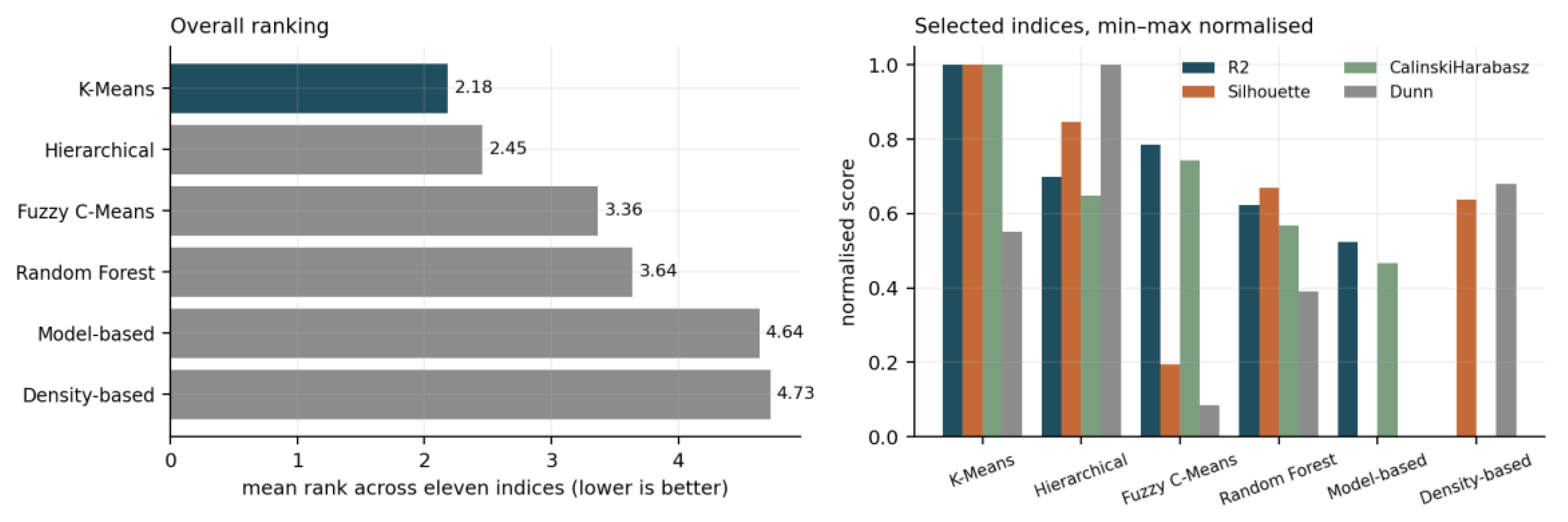
Density-based clustering was tuned over the same grid as in Appendix B.2 and retained a neighbourhood radius of 1.55 with a minimum neighbourhood size of four, yielding four clusters and leaving 42 of the 151 countries unassigned, or 27.8 per cent of the sample. Its indices are computed on the 109 assigned countries and are not directly comparable with those of the other algorithms. The comparison of the two blocks is instructive: the same algorithm classified 130 of 149 countries in the environmental space and only 109 of 151 here, which indicates that the social data contain a denser core and a more dispersed periphery, consistent with the small and extreme fourth cluster.
Figure A15.
The four clusters in the plane of the first two principal components, social block, with variable loadings shown as arrows.
Figure A15.
The four clusters in the plane of the first two principal components, social block, with variable loadings shown as arrows.
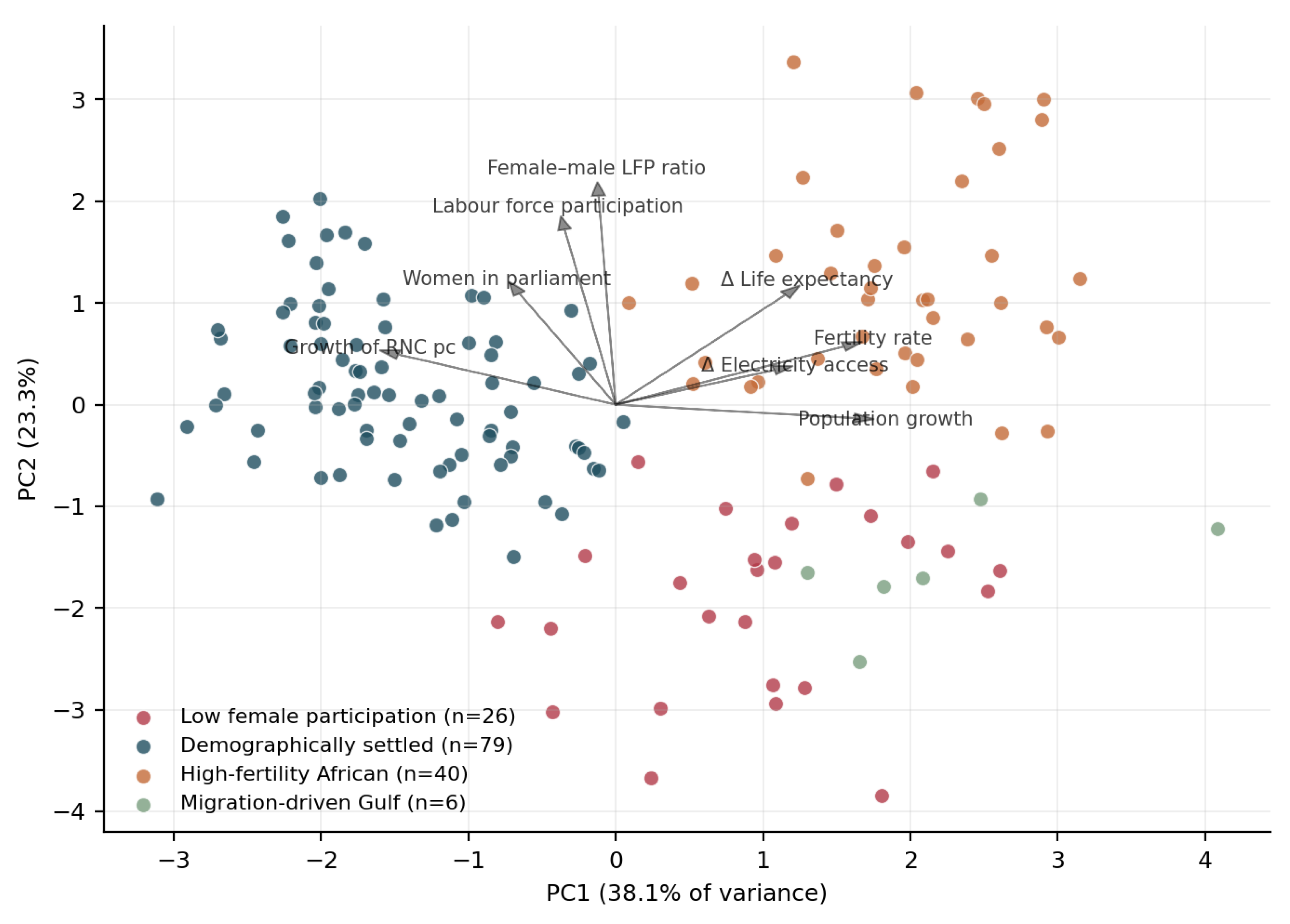
The first component, accounting for 38.1 per cent of the variance, is a demographic transition axis: it loads positively on population growth at 0.506, on fertility at 0.484, on the change in life expectancy at 0.360 and on the change in electricity access at 0.336, and negatively on the growth of renewable natural capital per capita at −0.461. It orders the settled economies, the low-participation group and the African group from left to right. The second component, at 23.3 per cent, is a female participation axis, loading on the female-to-male ratio at 0.642, on overall participation at 0.538 and on women in parliament at 0.341. It is what separates the low-participation group, which sits low on this axis, from the African group, which sits high on it despite occupying a similar position on the first. The Gulf cluster is distinguished by extreme values on the first axis combined with low values on the second.
Figure A16.
Left: distribution of silhouette widths within each cluster, social block. Right: mean growth of renewable natural capital per capita by cluster, with standard errors.
Figure A16.
Left: distribution of silhouette widths within each cluster, social block. Right: mean growth of renewable natural capital per capita by cluster, with standard errors.
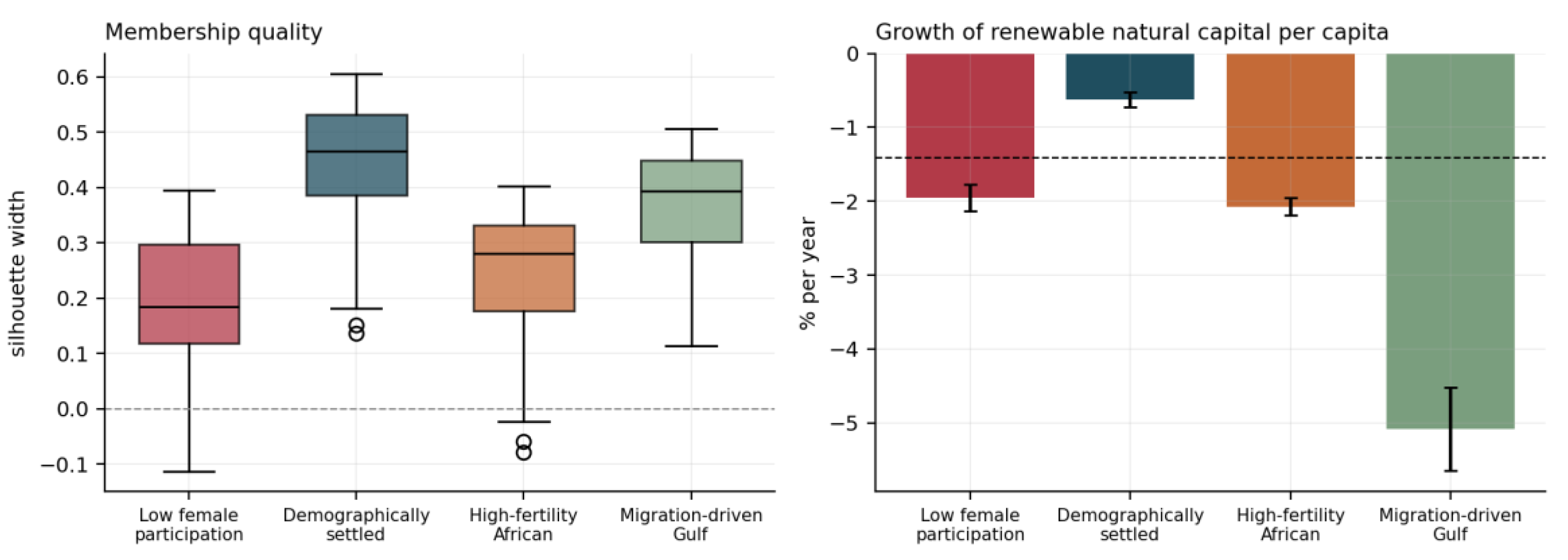
Table A17.
Cluster profiles in the original units of measurement, social block.
| Cluster | n | Growth of RNC pc (%) | Population growth | Fertility | Female–male LFP | Women in parliament | Representative members |
| Demographically settled | 79 | −0.62 | 0.54 | 1.84 | 74.0 | 21.7 | France, Germany, China, United States, Poland, Uruguay |
| Low female participation | 26 | −1.95 | 2.01 | 3.40 | 42.8 | 13.9 | India, Pakistan, Egypt, Morocco, Iran, Honduras |
| High-fertility African | 40 | −2.07 | 2.51 | 4.94 | 86.7 | 15.5 | Ethiopia, Tanzania, Uganda, Mali, Kenya, Ghana |
| Migration-driven Gulf | 6 | −5.08 | 4.69 | 2.27 | 49.2 | 5.8 | UAE, Qatar, Kuwait, Bahrain, Oman, Maldives |
Note. Population growth and fertility are annual rates and births per woman; participation ratios and parliamentary shares are percentages.
The demographically settled group is the most cohesive, with a mean silhouette of 0.443, followed by the Gulf group at 0.358, the African group at 0.239 and the low-participation group at 0.201. That the smallest cluster is also among the most cohesive confirms that it is a genuine type rather than a residual category. Only four countries have a negative silhouette width, all of them on the boundary between the settled and low-participation groups. Comparing the table row by row makes the substantive point of the section: the two middle groups differ by 44 percentage points in the female-to-male participation ratio and by 1.5 births per woman, yet their rates of natural capital accumulation differ by 0.12 percentage points, while the Gulf group, whose fertility is lower than either, loses natural capital two and a half times faster than both.
Appendix F. The S–Social Machine Learning Validation
Figure A17.
Left: cross-validated coefficient of determination by model, social block, folds grouped by country. Right: in-sample against cross-validated performance.
Figure A17.
Left: cross-validated coefficient of determination by model, social block, folds grouped by country. Right: in-sample against cross-validated performance.
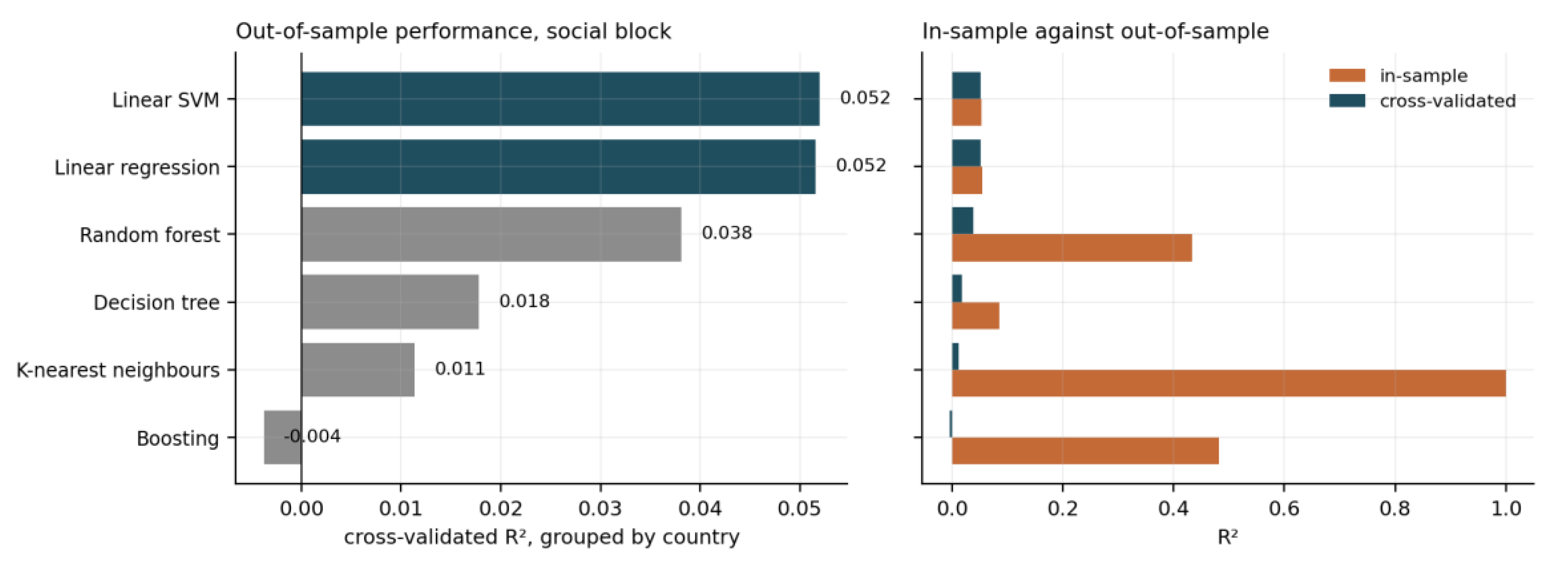
Hyperparameters are those of Appendix C.1, fixed rather than tuned, so that the two blocks are compared on identical settings. The negative cross-validated coefficient obtained by gradient boosting deserves a word, since it is unusual enough to invite the suspicion of an implementation error. It arises because the algorithm fits six hundred additive stages to a residualised series whose systematic component is roughly five per cent of its variance; each stage reduces the training loss and the accumulated adjustments do not transfer to countries held out of the training folds. Reducing the number of stages confirms the diagnosis: fifty stages return 0.0446 and one hundred return 0.0436, both positive but still below the linear model, and two hundred return 0.0296, so performance declines monotonically as the ensemble grows. This is the expected behaviour when the true conditional expectation is close to linear and weakly identified, and it means the negative figure in Table 11 reflects the fixed configuration rather than a defect of the algorithm.
Table A18.
Random forest attribution, social block.
| Regressor | Perm. share, pc | SHAP share, pc | SHAP share, total | Direction | FE coefficient | Bootstrap p |
| Population growth | 0.317 | 0.383 | 0.156 | −0.891 | −0.9132 | 0.0005 |
| Labour force participation | 0.142 | 0.128 | 0.146 | +0.381 | 0.0072 | 0.8080 |
| Δ Life expectancy | 0.117 | 0.107 | 0.145 | −0.256 | −0.0283 | 0.1905 |
| Fertility rate | 0.100 | 0.099 | 0.186 | +0.538 | 0.5368 | 0.0050 |
| Women in parliament | 0.117 | 0.099 | 0.132 | −0.266 | −0.0187 | 0.0825 |
| Female–male LFP ratio | 0.112 | 0.093 | 0.109 | +0.300 | 0.0106 | 0.5520 |
| Δ Electricity access | 0.096 | 0.091 | 0.127 | −0.110 | −0.0092 | 0.5650 |
Note. Shares are of the total mean absolute SHAP value; permutation importance uses twenty repetitions. The direction column refers to the per capita specification.
The permutation and SHAP rankings agree with each other on both definitions, as they did in the environmental block, and the correlation between the value of each regressor and its SHAP contribution has the same sign as the corresponding fixed-effects coefficient in every row. The magnitudes of those correlations are nonetheless informative: they are large for population growth at −0.891 and fertility at +0.538, the two coefficients that survived the bootstrap, and lie between 0.110 and 0.381 for the remaining five. The learner is using those five variables locally without any consistent directional effect, which is the algorithmic counterpart of an insignificant coefficient.
Figure A18.
Left: cross-validated performance of the linear model and the random forest under the two definitions of the dependent variable. Right: cross-validated performance of extended linear specifications on the per capita equation.
Figure A18.
Left: cross-validated performance of the linear model and the random forest under the two definitions of the dependent variable. Right: cross-validated performance of extended linear specifications on the per capita equation.
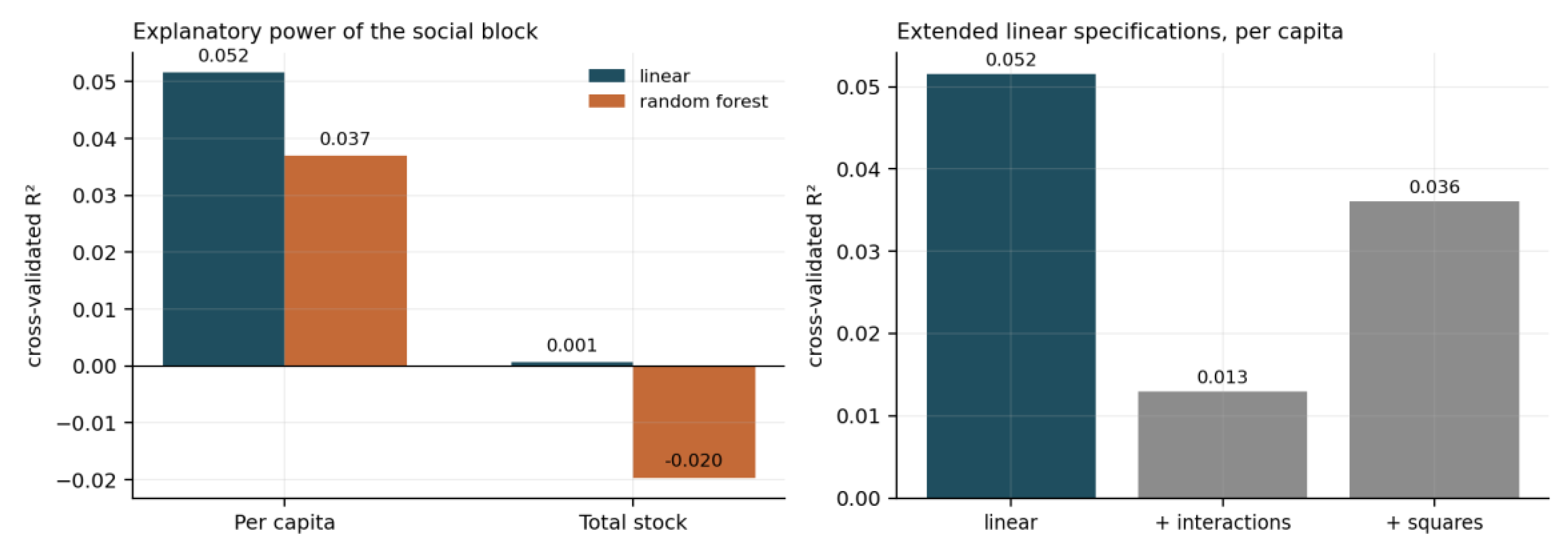
The left panel is the compact statement of the section. Moving from the per capita to the total definition of the dependent variable removes almost all explanatory power from the social block, for both the linear model and the flexible one, and the random forest becomes worse than the sample mean. The right panel shows that the loss cannot be recovered by enriching the functional form.
Table A19.
Partial dependence functions from the random forest, dependent variable in total.
| Regressor | Slope of the curve | Linear fit of the curve | Range of the curve |
| Fertility rate | +0.410 | 0.465 | 0.665 |
| Population growth | +0.060 | 0.089 | 0.391 |
| Women in parliament | −0.009 | 0.095 | 0.792 |
| Δ Electricity access | −0.012 | 0.169 | 0.202 |
Note. The linear fit is the coefficient of determination of a straight line through the partial dependence curve.
The fertility curve has a slope of 0.410, close to the fixed-effects coefficient of 0.537, but a linear fit of only 0.465, so it is visibly irregular. In the environmental block a comparable irregularity, on the renewable energy share, was interpreted as possible evidence of a threshold. That interpretation is not available here, because the model generating these curves has no out-of-sample validity: with a cross-validated coefficient of −0.020 the shape of its partial dependence functions is not evidence about the world. The curves are reported for completeness and for symmetry with Appendix C.3, and the correct reading is that they are uninformative.
Appendix G. The G–Governance Equation
The table explains why the fixed-effects column of Table 12 is nearly empty. Institutional quality carries 2.1 per cent of its variation within countries and its square 4.3 per cent, and agriculture value added 5.3 per cent; these are structural characteristics that barely move on an annual basis, and no estimator that discards the cross-section can say anything about them. Only three regressors are genuinely within-identified: the annual change in institutional quality at 92.9 per cent, GDP growth at 84.5 per cent and the change in internet penetration at 86.8 per cent. Reporting the fixed-effects and between estimators side by side is therefore not a robustness exercise in this block but the only way to read the results, and the appropriate summary is that the equation has a cross-sectional content and almost no temporal one.
Table A20.
Descriptive statistics, variance decomposition and variance inflation factors, 151 countries, 2003–2020, N = 2,629.
Table A20.
Descriptive statistics, variance decomposition and variance inflation factors, 151 countries, 2003–2020, N = 2,629.
| Variable | Mean | SD | Within share | VIF |
| Growth of renewable NC per capita (%) | −1.400 | 3.526 | 0.842 | — |
| Institutional quality (PC1, centred) | 0.067 | 2.256 | 0.021 | 2.33 |
| Institutional quality squared | 5.092 | 6.177 | 0.043 | 1.60 |
| Δ Institutional quality | 0.011 | 0.186 | 0.929 | 1.03 |
| Stability–effectiveness contrast (PC2) | −0.020 | 0.548 | 0.202 | 1.12 |
| GDP growth (%) | 3.492 | 4.710 | 0.845 | 1.05 |
| Δ Internet penetration (pp) | 2.772 | 3.379 | 0.868 | 1.09 |
| Agriculture value added (% of GDP) | 11.012 | 10.606 | 0.053 | 1.86 |
Figure A19.
Point estimates and 95 per cent confidence intervals by estimator, governance block.
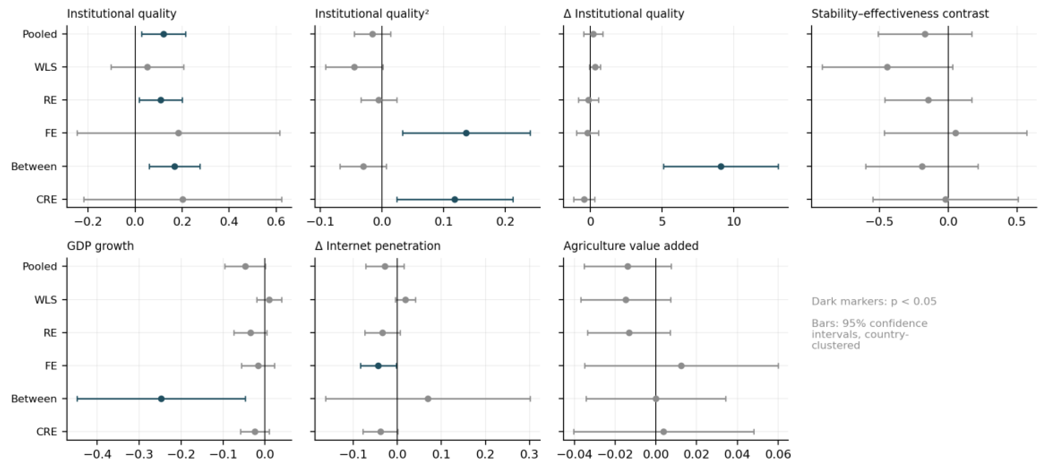
Table A21.
Mundlak specification and wild cluster bootstrap-t p-values, 1,999 replications with Rademacher weights and the null imposed.
Table A21.
Mundlak specification and wild cluster bootstrap-t p-values, 1,999 replications with Rademacher weights and the null imposed.
| Variable | Within term | Group-mean term | p on the group mean | FE coefficient | Bootstrap p |
| Institutional quality | 0.2025 | −0.0477 | 0.8411 | 0.1841 | 0.4300 |
| Institutional quality squared | 0.1178 | −0.1439 | 0.0038 | 0.1364 | 0.0090 |
| Δ Institutional quality | −0.4336 | 9.6202 | 0.0000 | −0.1984 | 0.6235 |
| Stability–effectiveness | −0.0192 | −0.1937 | 0.5485 | 0.0517 | 0.8485 |
| GDP growth | −0.0245 | −0.2315 | 0.0147 | −0.0166 | 0.4150 |
| Δ Internet penetration | −0.0386 | 0.1197 | 0.2923 | −0.0434 | 0.0275 |
| Agriculture value added | 0.0038 | −0.0027 | 0.9141 | 0.0125 | 0.5964 |
Note. Joint Wald test on the seven group means: 43.366, p < 0.001.
Three group-mean terms are significant and the joint test rejects decisively, so the between and within relationships differ for this block as they did for the environmental one. The pattern is nonetheless different in kind. In the environmental block the divergence concerned the renewable energy share, where the two dimensions carried opposite signs and both were significant; here the divergence is between a dimension that carries information and one that does not. No fixed-effects coefficient clears the Bonferroni threshold of 0.00714, and the two that come closest, the squared institutional term at 0.009 and the change in internet penetration at 0.028, are the ones for which no theoretical prior was specified in advance.
The negative coefficient on GDP growth in the between dimension, at −0.248 with a p-value of 0.017, is worth a comment because it is easily over-interpreted. Countries that grew faster over 2003–2020 accumulated renewable natural capital per capita more slowly, by 1.2 percentage points a year for a one standard deviation difference in average growth. This is consistent with the standard reading of the environmental Kuznets literature at the early stages of development, but it is equally consistent with the demographic mechanism of Section 7, since fast-growing economies in this sample are disproportionately those with high population growth. The specification cannot separate the two.
Table A22.
The institutional coefficients under alternative definitions of the dependent variable, two-way fixed effects with country-clustered standard errors.
Table A22.
The institutional coefficients under alternative definitions of the dependent variable, two-way fixed effects with country-clustered standard errors.
| Dependent variable | Institutional quality | Δ Institutional quality | Institutional quality2 | N |
| Renewable NC per capita | 0.1841 | −0.1984 | 0.1364*** | 2,629 |
| Total renewable NC | 0.2489 | −0.1304 | 0.1316*** | 2,629 |
| Excluding agricultural land, per capita | 0.0779 | −0.4871 | 0.2052 | 2,625 |
Unlike the social block, the governance coefficients are essentially unchanged when the per capita denominator is removed, which confirms that no accounting identity is operating here. The squared institutional term is 0.136 on the per capita measure and 0.132 on the total, and the level term moves from 0.184 to 0.249 while remaining insignificant in both. Restricting the dependent variable to the components other than agricultural land leaves all three coefficients insignificant with wider standard errors, as expected given the smaller and noisier base.
Table A23.
Specification tests, governance block, N = 2,629.
| Test | Statistic | p-value | Comparison across the three blocks |
| F test on country effects | 2.867 | < 0.001 | Significant in E and G, not in S |
| Hausman, FE against RE | 45.653 | < 0.001 | Rejects in E and G, not in S |
| Breusch–Pagan LM | 193.988 | < 0.001 | Significant in all three |
| Mundlak joint test | 43.366 | < 0.001 | Decisive in E and G, borderline in S |
| Wooldridge test for AR(1) | −0.192 | 0.040 | Absent in E, present in S and G |
| Pesaran CD | 3.062 | 0.002 | Present in all three, mean absolute ρ 0.206 |
Table A24.
Shift-share instrumental variable estimates, governance block.
| Endogenous regressor | First-stage F | FE estimate | 2SLS estimate | Wu–Hausman p |
| Institutional quality | 21.14 | 0.1841 (0.2200) | −1.2923 (1.3419) | 0.361 |
| Δ Internet penetration | 45.50 | −0.0434 (0.0207) | −0.1347 (0.0810) | 0.247 |
| Agriculture value added | 28.22 | 0.0125 (0.0243) | 0.1252 (0.0734) | 0.088 |
Note. Standard errors clustered by country in parentheses.
All three instruments are relevant by the conventional threshold and none of the three second-stage estimates is significant at the five per cent level. The Wu–Hausman tests do not reject exogeneity for institutional quality or internet penetration and reject only marginally for agriculture value added. The honest summary is that instrumentation confirms the null results of the fixed-effects specification without adding information, which is unsurprising given that the equation’s explanatory content lies in a dimension the instruments do not reach. The exercise is reported because a governance equation that did not address the endogeneity of institutions would be incomplete, not because it changes any conclusion.
Appendix H. The G–Governance Clustering
Appendix H.1
. Selection of the Number of Clusters
Figure A20.
Selection of the number of clusters, governance block. Left: average silhouette width. Centre: explained variance. Right: marginal reduction in within-cluster deviance.
Figure A20.
Selection of the number of clusters, governance block. Left: average silhouette width. Centre: explained variance. Right: marginal reduction in within-cluster deviance.
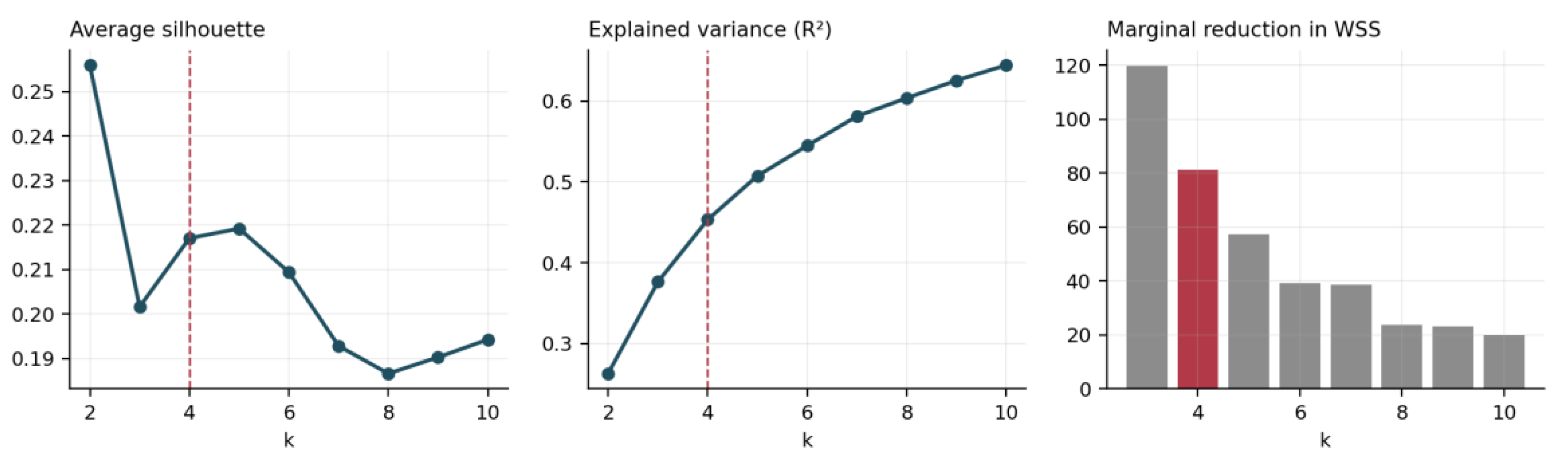
Table A25.
Selection statistics for the k-means solution on the governance block, k from 2 to 10, 151 countries.
Table A25.
Selection statistics for the k-means solution on the governance block, k from 2 to 10, 151 countries.
| k | R2 | Silhouette | Calinski–Harabasz | AIC | BIC | Within deviance | Marginal reduction |
| 2 | 0.263 | 0.256 | 53.15 | −290.4 | −242.2 | 779.1 | — |
| 3 | 0.376 | 0.202 | 44.63 | −450.8 | −378.4 | 659.4 | 119.7 |
| 4 | 0.453 | 0.217 | 40.59 | −573.9 | −477.3 | 578.1 | 81.3 |
| 5 | 0.507 | 0.219 | 37.59 | −668.3 | −547.6 | 520.8 | 57.3 |
| 6 | 0.545 | 0.209 | 34.67 | −735.3 | −590.4 | 481.4 | 39.3 |
| 7 | 0.581 | 0.193 | 33.28 | −807.4 | −638.5 | 442.9 | 38.5 |
| 8 | 0.603 | 0.187 | 31.08 | −849.6 | −656.5 | 419.2 | 23.7 |
| 9 | 0.625 | 0.190 | 29.61 | −893.4 | −676.2 | 396.1 | 23.1 |
| 10 | 0.644 | 0.194 | 28.35 | −931.9 | −690.5 | 376.2 | 19.9 |
The silhouette profile of this block is the least decisive of the three: the range from k = 3 to k = 10 spans only 0.187 to 0.219, so the criterion cannot discriminate among solutions, and the value at k = 5 marginally exceeds that at k = 4. The five-cluster solution was inspected and splits the third group into two subgroups distinguished by GDP growth rather than by anything institutional, adding no interpretable content; four clusters were retained on that basis together with the deviance elbow.
Figure A21.
Left: mean rank across the eleven internal validity indices, governance block. Right: four selected indices, min–max normalised.
Figure A21.
Left: mean rank across the eleven internal validity indices, governance block. Right: four selected indices, min–max normalised.
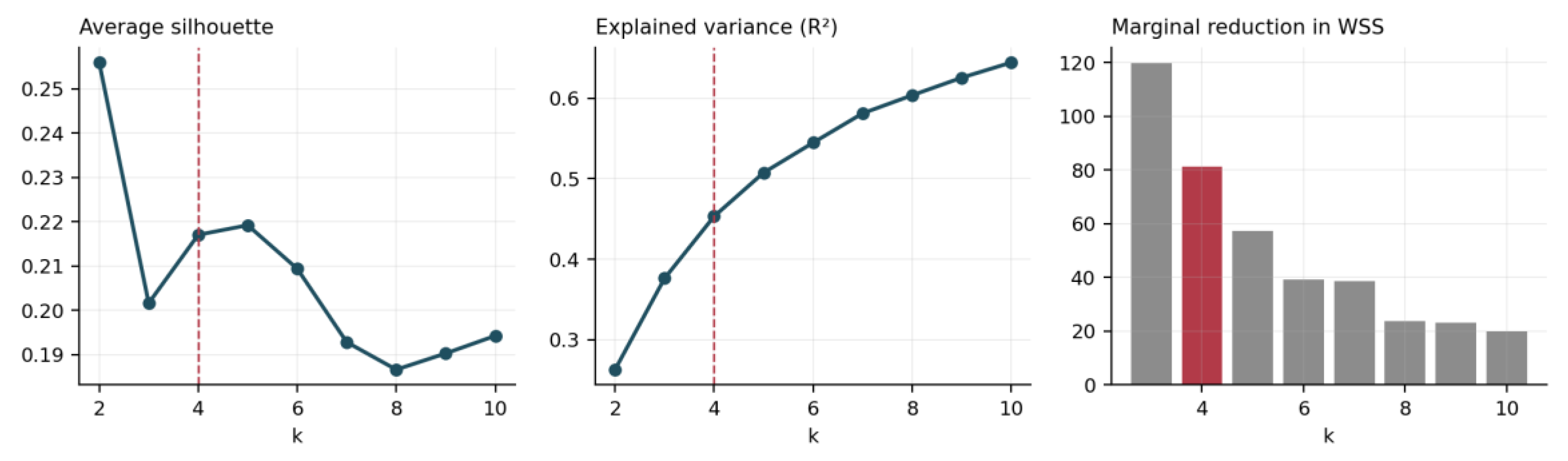
The tuning of the density-based method followed Appendices B.2 and E.2 and retained a neighbourhood radius of 1.40 with a minimum neighbourhood size of four, producing four clusters and leaving 49 countries unassigned. Comparing the three blocks on this single algorithm is instructive: it classified 130 of 149 countries in the environmental space, 109 of 151 in the social space and 102 of 151 here, with silhouette values of 0.223, 0.266 and 0.029 respectively. The monotone deterioration tracks the extent to which each block of variables is continuously rather than discretely distributed across countries, and the governance block is the most continuous of the three.
Figure A22.
The four clusters in the plane of the first two principal components, governance block, with variable loadings shown as arrows.
Figure A22.
The four clusters in the plane of the first two principal components, governance block, with variable loadings shown as arrows.
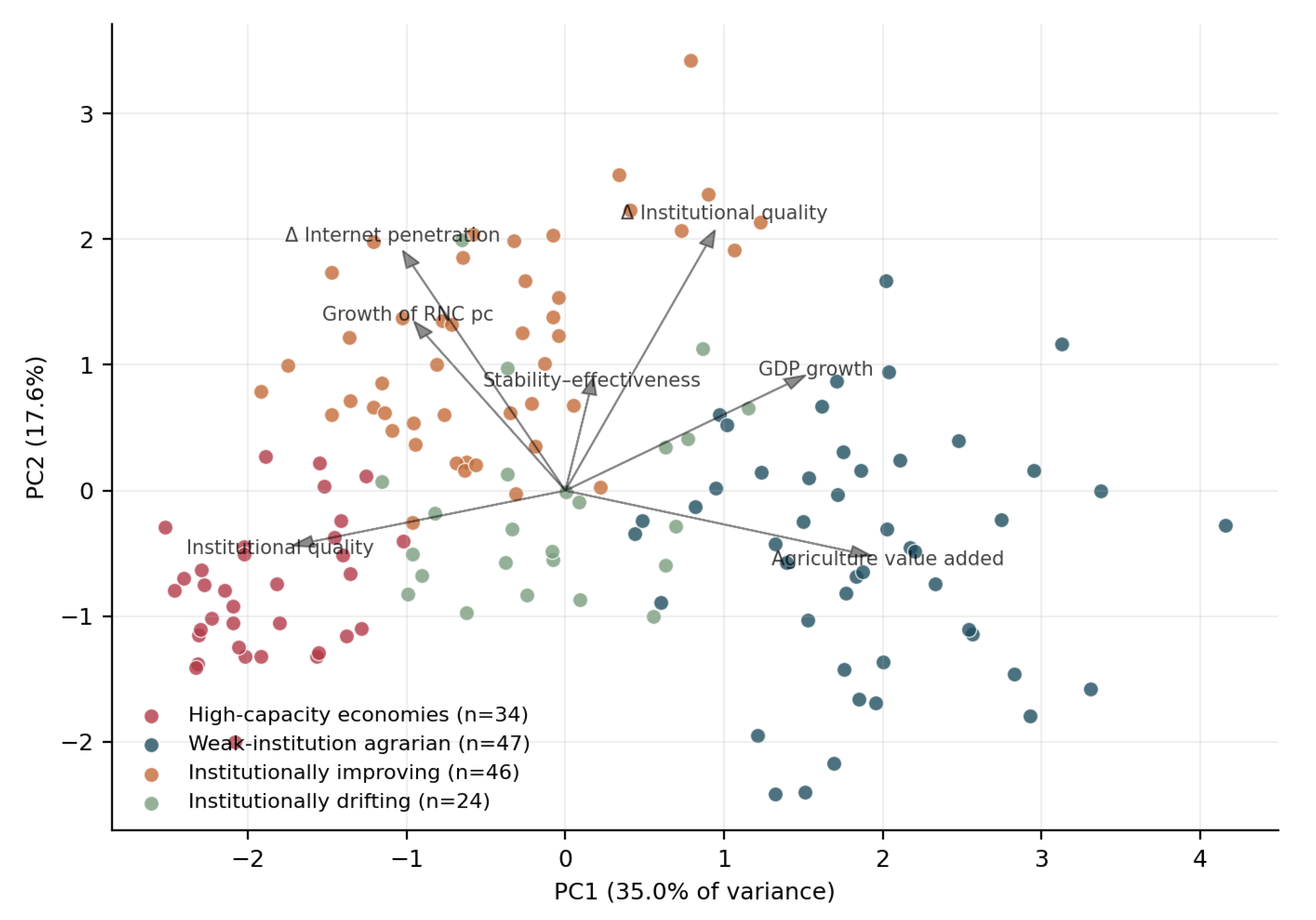
The first component, at 35.0 per cent of the variance, is a development axis: it loads positively on agriculture value added at 0.563 and GDP growth at 0.437, and negatively on institutional quality at −0.498, the change in internet penetration at −0.301 and the growth of renewable natural capital at −0.274. It separates the high-capacity economies from the weak-institution agrarian ones. The second component, at 17.6 per cent, is a trajectory axis: it loads on the change in institutional quality at 0.609, the change in internet penetration at 0.559 and the growth of the dependent variable at 0.386. It is what distinguishes the institutionally improving group from the institutionally drifting one, which occupy the same region of the first axis. The classification is genuinely two-dimensional, and a ranking of countries by institutional level alone would place the third and fourth groups together.
Figure A23.
Left: distribution of silhouette widths within each cluster, governance block. Right: mean growth of renewable natural capital per capita by cluster, with standard errors.
Figure A23.
Left: distribution of silhouette widths within each cluster, governance block. Right: mean growth of renewable natural capital per capita by cluster, with standard errors.
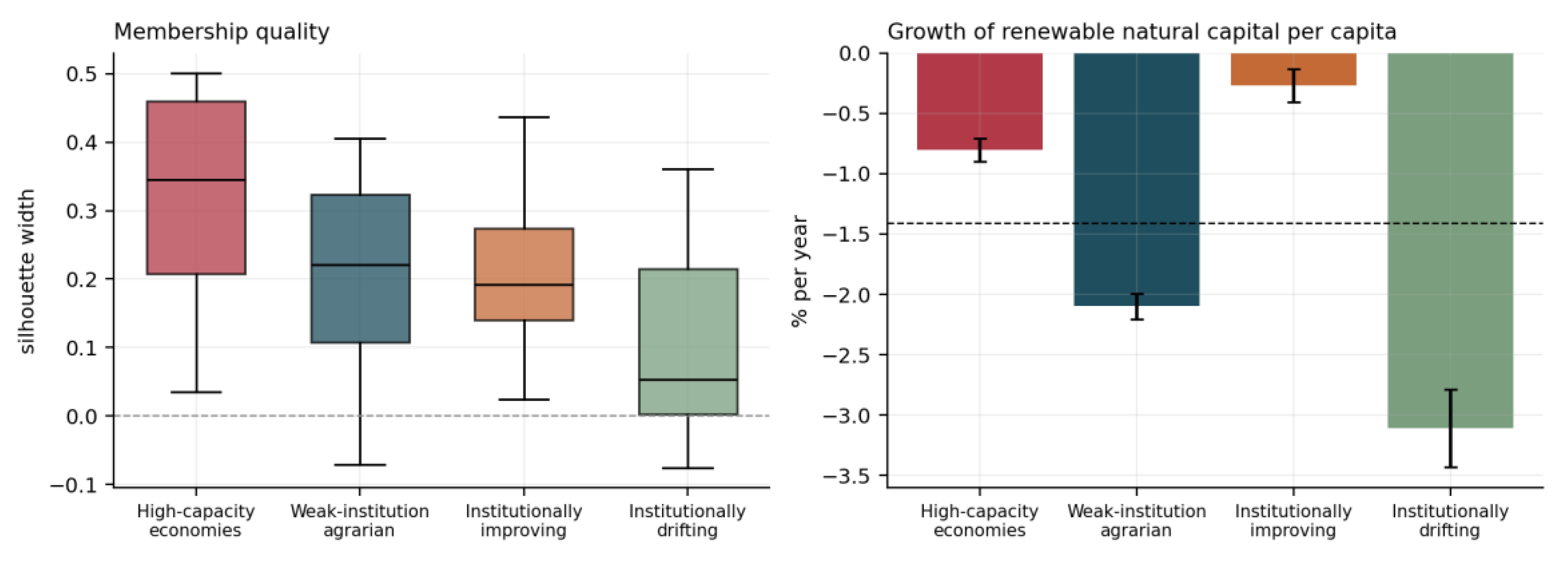
Table A26.
Cluster profiles in the original units of measurement, governance block, ordered by rate of accumulation.
Table A26.
Cluster profiles in the original units of measurement, governance block, ordered by rate of accumulation.
| Cluster | n | Growth of RNC pc (%) | Institutional quality | Cumulative Δ institutional quality | Agriculture (% GDP) | Representative members |
| High-capacity economies | 34 | −0.80 | 2.87 | −0.55 | 2.3 | Germany, Canada, Japan, Sweden, Australia, France |
| Institutionally improving | 46 | −0.27 | 0.11 | +0.72 | 7.1 | Romania, Lithuania, Armenia, Viet Nam, Peru, Serbia |
| Weak-institution agrarian | 47 | −2.10 | −1.99 | +0.47 | 23.5 | Niger, Uganda, Tanzania, Kenya, Nigeria, Ethiopia |
| Institutionally drifting | 24 | −3.11 | −0.26 | −0.28 | 6.9 | Kuwait, UAE, Iran, Gabon, Bolivia, Guatemala |
Note. The cumulative change in institutional quality is the mean annual change multiplied by the eighteen years of the sample.
Ordering the table by outcome rather than by institutional level makes the pattern visible. The two groups at the extremes of institutional quality, at 2.87 and −1.99, occupy the second and third positions in the ranking by natural capital accumulation, while the first and last positions are taken by two groups whose institutional levels differ by 0.37 index points and whose institutional trajectories differ by a full index point over the period. Whatever the direction of causation, the level of institutional quality is not what orders these countries; the direction of institutional change is closer to doing so, though the confounding with the demographic mechanism of Section 8 is not resolved.
The mean silhouette by cluster is 0.322 for the high-capacity economies, 0.212 for the institutionally improving group, 0.203 for the weak-institution agrarian group and 0.105 for the institutionally drifting group. The last value is low enough that the fourth group should be treated as a loose collection of countries sharing a negative institutional trajectory rather than as a tightly defined type, which is consistent with its heterogeneous membership, spanning Gulf hydrocarbon exporters, Andean middle-income economies and Central American ones.
Appendix I. The G–Governance Machine Learning Validation
The within run reproduces the design of Appendices C.1 and F.1 exactly: the dependent variable and the seven regressors are residualised on country and year effects by iterated demeaning, cross-validation uses ten folds constructed by country, and hyperparameters are fixed at the values used in the other two blocks so that the three are comparable.
The between run operates on the 151 country means of the same variables. Two details of its construction should be recorded. The squared institutional term is computed as the square of the country mean rather than as the mean of the squares, since the object being modelled is the cross-sectional relationship and the two differ by the within-country variance of the index. Cross-validation uses ten random folds rather than grouped folds, since each observation is already a distinct country and there is no grouping structure left to respect. The neighbourhood size for k-nearest neighbours was reduced from twenty-five to ten and the tree depth from six to four, because the original settings are inappropriate for a sample of 151; no other hyperparameter was altered.
Table A27.
Cross-validated performance over ten random ten-fold partitions of the 151 country means.
Table A27.
Cross-validated performance over ten random ten-fold partitions of the 151 country means.
| Model | Mean CV R2 | SD across splits | Minimum | Maximum |
| Random forest | 0.2877 | 0.0154 | 0.2655 | 0.3128 |
| Linear regression | 0.1073 | 0.0179 | 0.0775 | 0.1320 |
Note. The random forest is ahead of the linear model in ten partitions out of ten.
The single-split figures reported in Table 15 are conservative relative to this distribution, since the seed used there returns 0.2172 for the random forest against a mean of 0.2877 across ten seeds. The ordering is invariant, and the gap between the two models, at 0.18 on average, is an order of magnitude larger than its variability across partitions. The claim that flexibility helps in the between dimension is therefore robust to the partition, though it remains subject to the small sample.
Table A28.
Random forest attribution on the 151 country means.
| Regressor | Perm. share | SHAP share | SHAP direction | Between coefficient | FE coefficient | Signs agree |
| GDP growth | 0.187 | 0.192 | −0.737 | −0.2475 | −0.0166 | Yes |
| Agriculture value added | 0.240 | 0.192 | −0.167 | 0.0000 | 0.0125 | No sign |
| Δ Institutional quality | 0.164 | 0.185 | +0.887 | 9.0956 | −0.1984 | Yes |
| Δ Internet penetration | 0.185 | 0.183 | +0.458 | 0.0688 | −0.0434 | Yes |
| Institutional quality | 0.143 | 0.171 | +0.857 | 0.1666 | 0.1841 | Yes |
| Stability–effectiveness | 0.047 | 0.048 | −0.392 | −0.1916 | 0.0517 | Yes |
| Institutional quality2 | 0.034 | 0.031 | −0.025 | −0.0308 | 0.1364 | Yes |
Note. Permutation importance uses fifty repetitions and the mean squared error as scoring function. The direction is the correlation between the value of the regressor and its SHAP contribution.
Permutation importance and SHAP agree on the ordering except for agriculture value added, which ranks first on permutation importance at 24.0 per cent and second on SHAP at 19.2 per cent. The discrepancy is informative: permutation importance measures the accuracy lost when a variable is scrambled and is therefore sensitive to a variable that the model uses locally in many places, while SHAP measures the average magnitude of its contribution. Agriculture value added is used by the forest to separate the low-income group of countries from the rest, a role that costs accuracy when removed but does not produce a large average directional contribution — its SHAP direction is only −0.167.
The two variables with the smallest attributed importance, the stability–effectiveness contrast at 4.8 per cent and the squared institutional term at 3.1 per cent, are also the two that the between estimator leaves insignificant, so the algorithm and the econometrics agree on what does not matter as well as on what does.
Figure A24.
Partial dependence functions from the random forest estimated on country means, with the least-squares line through each curve shown as a dashed line.
Figure A24.
Partial dependence functions from the random forest estimated on country means, with the least-squares line through each curve shown as a dashed line.
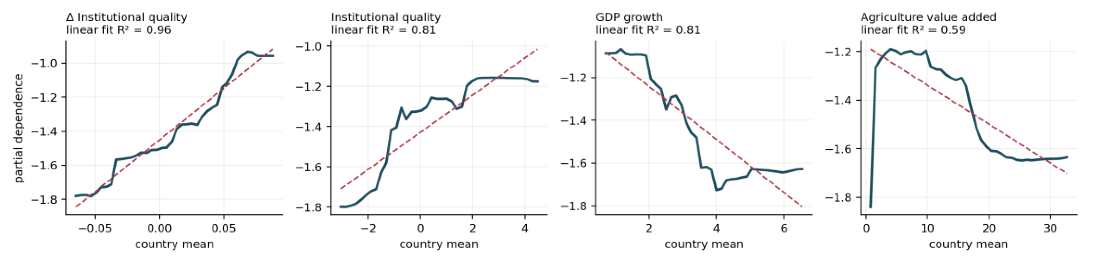
Table A29.
Out-of-sample performance of extended linear specifications and of the random forest on the 151 country means.
Table A29.
Out-of-sample performance of extended linear specifications and of the random forest on the 151 country means.
| Specification | Cross-validated R2 | Change from baseline |
| Linear, seven regressors | 0.1090 | — |
| Adding twenty-one interactions | 0.0167 | −0.0923 |
| Adding seven squared terms | 0.0265 | −0.0825 |
| Random forest | 0.2172 | +0.1082 |
The table isolates the puzzle discussed in the body of the section. Both parametric extensions of the linear model reduce performance sharply, which is the expected consequence of estimating twenty-one or seven additional parameters on 151 observations, while the nonparametric alternative doubles it. The partial dependence curves show that the marginal relationships are close to linear individually, with linear fits of 0.964 for the change in institutional quality, 0.815 for its level and 0.808 for GDP growth, and only agriculture value added displays appreciable irregularity at 0.586.
The most plausible reconciliation is that the forest is exploiting local structure rather than global curvature: it partitions the sample into groups of countries within which different variables matter, which is a form of flexibility that adding polynomial terms to a single global equation cannot represent and that a small sample cannot support if it is imposed parametrically. This is precisely the structure the clustering of Section 11 describes, and the two results should be read together. A formal test would require estimating a threshold or a finite mixture model on the cross-section, which 151 observations do not comfortably support, and is left for future work.
Appendix J. Variables, Acronyms and Source Codes
Every variable used in this study is drawn from the Sovereign ESG Data Portal of the World Bank. The tables below give, for each variable, the acronym used throughout the paper, the source code under which the series is published, the official indicator name, the transformation applied, and a one-line description. The final column reports the within-country share of total variation over the relevant estimation sample, which determines whether a coefficient on that variable is identified mainly by the fixed-effects or by the between estimator.
Table A30.
The dependent variable and the components of the renewable natural capital account.
| Code | Series | Indicator and transformation | Description | Within |
| gRNC | NW.NCA.TOTL.PC | Renewable natural capital per capita, total — 100 × δln | Dependent variable throughout. Net investment of a nation in its renewable natural asset base, in percentage points per year | 0.860 |
| gRNCtot | NW.NCA.TOTL.PC + SP.POP.GROW | As above, plus population growth — 100 × δln + population growth | Growth of the total rather than the per capita stock, used in Section 7 to remove the accounting identity | 0.962 |
| — | NW.NCA.AGRI.PC | Renewable natural capital, agricultural land | Largest component, 62.1 per cent of the aggregate on average; used in the decomposition of Section 4.6 and Section 7 | — |
| — | NW.NCA.FTIM.PC | Renewable natural capital, timber | Second component, 9.9 per cent | — |
| — | NW.NCA.FSTW.PC | Forest water ecosystem services | 7.9 per cent | — |
| — | NW.NCA.HYDR.PC | Hydropower energy | 6.9 per cent | — |
| — | NW.NCA.FSTC.PC | Forest recreation, hunting and fishing services | 6.4 per cent | — |
| — | NW.NCA.FSTP.PC | Nonwood forest protection ecosystem services | 2.7 per cent | — |
| — | NW.NCA.MANG.PC | Mangroves | 2.2 per cent | — |
| — | NW.NCA.FISH.PC | Fisheries | Smallest component, 2.0 per cent | — |
| — | NW.TOW.PC | National comprehensive wealth per capita | Denominator of the wealth-share statistics reported in Section 4 | — |
Note. All series are drawn from the Changing Wealth of Nations accounts within the World Bank Sovereign ESG Data Portal and measured in real chained 2019 US dollars. Component shares are averages over the sample period and sum to the aggregate. The final column reports the within-country share of total variation, computed on the environmental estimation sample.
The eight components sum to the aggregate, and their shares are the basis of the accounting decompositions that distinguish valuation effects from economic ones. Nonrenewable natural capital, published as NW.NCA.SSOI.PC, is not part of the dependent variable and is reported here only because it is referenced in the discussion of the arid hydrocarbon cluster.
Table A31.
The environmental block.
| Code | Series | Indicator and transformation | Description | Within |
| DFRST | AG.LND.FRST.ZS | Forest area (% of land area) — first difference | Annual change in forest cover, in percentage points of total land area | 0.488 |
| DAGRI | AG.LND.AGRI.ZS | Agricultural land (% of land area) — first difference | Annual change in cultivated and pasture area; largest coefficient in the block, five sixths of it an accounting channel | 0.918 |
| DFOR | NY.ADJ.DFOR.GN.ZS | Adjusted savings, net forest depletion (% of GNI) | Value of timber harvest in excess of natural regeneration, relative to national income | 0.136 |
| DRES | NY.ADJ.DRES.GN.ZS | Adjusted savings, natural resources depletion (% of GNI) | Total rents from energy, mineral and forest depletion; predominantly subsoil in most countries | 0.160 |
| SPEI | EN.CLC.SPEI.XD | Standardised Precipitation-Evapotranspiration Index | Climatic water balance; higher values denote wetter conditions and lower values drought. The only regressor with a strong claim to exogeneity | 0.873 |
| DNST | EN.POP.DNST | Population density (people per sq. km) — natural logarithm | Structural pressure on land; almost no within-country variation, so interpretable only across countries | 0.011 |
| RNEW | EG.FEC.RNEW.ZS | Renewable energy consumption (% of final energy) | Includes traditional biomass, which is why the coefficient reverses sign between the two panel dimensions | 0.028 |
Note. Seven regressors drawn from the World Bank Sovereign ESG Data Portal and entered in the equations of Section 4 to 6. The final column reports the within-country share of total variation over the estimation sample of 3,611 observations on 149 countries, 1996–2020; variables below roughly 0.3 carry most of their information across countries and their fixed-effects coefficients should not be interpreted.
Table A32.
The social block.
| Code | Series | Indicator and transformation | Description | Within |
| POPG | SP.POP.GROW | Population growth (annual %) | Enters the per capita dependent variable through the denominator by construction; its coefficient is the accounting identity | 0.286 |
| TFRT | SP.DYN.TFRT.IN | Fertility rate, total (births per woman) | The one social variable surviving the change of dependent variable; operates through the agricultural land component | 0.045 |
| DLE | SP.DYN.LE00.IN | Life expectancy at birth (years) — first difference | Annual change in life expectancy, a flow measure of health improvement | 0.975 |
| LFPR | SL.TLF.ACTI.ZS | Labour force participation rate, ages 15–64 (%) | Modelled ILO estimate; between-identified | 0.049 |
| FMLF | SL.TLF.CACT.FM.ZS | Ratio of female to male participation (%) | Defining variable of the low-participation cluster of Section 8 | 0.042 |
| DELEC | EG.ELC.ACCS.ZS | Access to electricity (% of population) — first difference | Annual pace of electrification, in percentage points | 0.863 |
| PARL | SG.GEN.PARL.ZS | Seats held by women in national parliaments (%) | Political representation; marginally significant under fixed effects but not after the bootstrap | 0.282 |
Note. Seven regressors drawn from the World Bank Sovereign ESG Data Portal and entered in the equations of Section 7 to 9. The final column reports the within-country share of total variation over the estimation sample of 3,293 observations on 151 countries, 1997–2020. Population growth enters the per capita dependent variable by construction, so its coefficient is interpreted against the value of −1 implied by the accounting identity rather than as a behavioural effect.
The six Worldwide Governance Indicators correlate between 0.73 and 0.95 and cannot be entered jointly, since doing so produces variance inflation factors up to 23.1. They are replaced by their first two principal components, described in the second table below.
Table A33.
The six Worldwide Governance Indicators.
| Code | Series | Indicator | Range | Description |
| RL | GOV_WGI_RL.EST | Rule of Law | −2.5 to +2.5 | Confidence in and abidance by the rules of society |
| CC | GOV_WGI_CC.EST | Control of Corruption | −2.5 to +2.5 | Extent to which public power is exercised for private gain |
| GE | GOV_WGI_GE.EST | Government Effectiveness | −2.5 to +2.5 | Quality of public services and policy implementation |
| RQ | GOV_WGI_RQ.EST | Regulatory Quality | −2.5 to +2.5 | Ability to formulate regulations permitting private-sector development |
| VA | GOV_WGI_VA.EST | Voice and Accountability | −2.5 to +2.5 | Participation in selecting government, freedom of expression and association |
| PV | GOV_WGI_PV.EST | Political Stability | −2.5 to +2.5 | Likelihood of political instability or politically motivated violence |
Note. All series are drawn from the World Bank Sovereign ESG Data Portal and are estimates on a standard normal scale, with higher values denoting better outcomes. Their pairwise correlations range from 0.73 to 0.95 with a mean of 0.85, and entering them jointly produces variance inflation factors up to 23.1, so they are not used directly: the governance equation is estimated on their first two principal components.
The first principal component of these six accounts for 87.7 per cent of their joint variance and loads almost uniformly on all of them, between 0.374 and 0.428; the second accounts for a further 5.3 per cent and is dominated by political stability, on which it loads at 0.900, against negative loadings on government effectiveness and regulatory quality. The governance equation is estimated on the following seven regressors.
Table A34.
The governance block.
| Code | Series | Indicator and transformation | Description | Within |
| IQ | Six WGI series | Institutional quality — first principal component, centred | General index of institutional development; between-identified | 0.021 |
| IQ2 | Six WGI series | Institutional quality squared — square of iq | Allows a non-monotonic relationship; the coefficient changes sign between dimensions | 0.043 |
| DIQ | Six WGI series | Change in institutional quality — first difference of iq | Reform trajectory rather than level; the coefficient that dominates the between dimension | 0.929 |
| DEM | Six WGI series | Stability–effectiveness contrast — second principal component | Extent to which political stability exceeds administrative capacity | 0.202 |
| GDPG | NY.GDP.MKTP.KD.ZG | GDP growth (annual %) | Rate of economic expansion | 0.845 |
| DNET | IT.NET.USER.ZS | Individuals using the internet (% of population) — first difference | Annual pace of digital diffusion, in percentage points | 0.868 |
| AGVA | NV.AGR.TOTL.ZS | Agriculture, forestry and fishing, value added (% of GDP) | Structural weight of the primary sector | 0.053 |
Note. Seven regressors entered in the equations of Section 10 to 12. The first four are constructed from the six Worldwide Governance Indicators of Table J.4: the first principal component accounts for 87.7 per cent of their joint variance and loads almost uniformly on all six, between 0.374 and 0.428, while the second accounts for a further 5.3 per cent and is dominated by political stability, loading at 0.900 against negative loadings on government effectiveness and regulatory quality. The final column reports the within-country share of total variation over the estimation sample of 2,629 observations on 151 countries, 2003–2020.
NY.GDP.PCAP.CD, GDP per capita in current US dollars, enters in logarithms as a control in the robustness specifications of Appendix A.2 and defines the income splits reported in Appendices A.6 and D.3. It is not part of any pillar block.
The following abbreviations recur in the text and tables. OLS, ordinary least squares; WLS, weighted least squares; RE, random effects; FE, fixed effects, applied throughout with both country and year effects; CRE, correlated random effects in the Mundlak formulation, in which the group means of the regressors are added to a random effects specification; LSDV, least squares with dummy variables, used for the dynamic specifications; 2SLS, two-stage least squares. SPEI is the Standardised Precipitation-Evapotranspiration Index; WGI, the Worldwide Governance Indicators; PC1 and PC2, the first and second principal components. SHAP denotes Shapley additive explanations, and CV cross-validation, performed throughout with folds grouped by country. Cluster validity indices are abbreviated as CH for Calinski–Harabasz and HHI for the Herfindahl–Hirschman index of the cluster size distribution.
Within shares are computed on the estimation sample of the block in which each variable appears, and differ marginally across blocks for the dependent variable because the three samples are not identical: 3,611 observations on 149 countries for the environmental block, 3,293 on 151 for the social, and 2,629 on 151 for the governance.
References
- Abd El Nasser, N.; Ibrahiem, D.M.; Sameh, R. The nexus between the dependence on natural resources and environmental sustainability: Does institutional matter? Resour. Policy 2025, 101, 105466. [Google Scholar] [CrossRef]
- Abou Houran, M.; Mehmood, U. How institutional quality and renewable energy interact with ecological footprints: do the human capital and economic complexity matter in the Next Eleven nations? In Environmental Science and Pollution Research; 2023. [Google Scholar] [CrossRef]
- Achahboun, C.; Chikhaoui, M.; Naimi, M.; Bellafkih, M.; Bassairate, O. Comparative Assessment of Transformer and Conventional Deep Learning Models for Dam Inflow Prediction. Water Resour. Manag. 2026, 40(9), 429. [Google Scholar] [CrossRef]
- Adikpo, J.A.; Usman, O. Moving towards the path of environmental sustainability in Developing-8 countries: investigating the role of country’s reputation in mitigating environmental externalities. Environ. Sci. Pollut. Res. 2023, 30(50), 109784–109799. [Google Scholar] [CrossRef]
- Agarwal, P.; Sawhney, A. Sustainability and comprehensive wealth accounting: the case of India. Environ. Dev. Sustain. 2021, 23(3), 3762–3786. [Google Scholar] [CrossRef]
- Ahmad, N.; Derrible, S.; Managi, S. A network-based frequency analysis of Inclusive Wealth to track sustainable development in world countries. J. Environ. Manag. 2018, 218, 348–354. [Google Scholar] [CrossRef]
- Ahmad, I.; Khokale, R.; Gongal, N. Performance assessment of linear regression for crop yield prediction in comparison with contemporary models. Bull. Electr. Eng. Inform. 2026, 15(4), 3762–3771. [Google Scholar] [CrossRef]
- Ahmed, T.; Jahan, I. Geospatial simulation of land use change and ecosystem services in Chattogram, Bangladesh using PLUS model (2000–2060). Int. J. Environ. Sci. Technol. 2026, 23(1), 33. [Google Scholar] [CrossRef]
- AL-Barakani, A.; Bin, L.; Zhang, X.; Saeed, M.; Qahtan, A.S.A.; Hamood Ghallab, H.M. Spatial analysis of financial development’s effect on the ecological footprint of belt and road initiative countries: Mitigation options through renewable energy consumption and institutional quality. J. Clean. Prod. 2022, 366, 132696. [Google Scholar] [CrossRef]
- Alnaqbi, A.; Al-Khateeb, G.G.; Zeiada, W. Hybrid machine learning framework for transverse cracking prediction in CRCP with PSO and GBM. Urban Lifeline 2026, 4(1), 5. [Google Scholar] [CrossRef]
- Alsaleh, M.; Abdul-Rahim, A.S. Does hydropower growth threaten fish security under the pathway of sustainable development? Evidence from European Union economies. Energy Environ. 2023, 34(1), 78–98. [Google Scholar] [CrossRef]
- Al-Tahat, S.; Bani-Khaled, S.; Jaradat, Z.; Mansour, M.; Al-zoubi, A.M. State ownership as a moderator in the relationship between board characteristics and ESG performance: evidence from Asia-Pacific markets. J. Bus. Socio-Econ. Dev. 2025, 1–22. [Google Scholar] [CrossRef]
- Aly, E.A.; Managi, S. Energy infrastructure and their impacts on societies’ capital assets: A hybrid simulation approach to inclusive wealth. Energy Policy 2018, 121, 1–12. [Google Scholar] [CrossRef]
- Amare, M.Z.; Mulugeta, W.; Mencha, M. Nexus between natural resource endowments and economic growth in selected African countries. Discov. Sustain. 2024, 5(1), 255. [Google Scholar] [CrossRef]
- Ameer, W.; Ahmad, K. How wealthy in natural resource leads environmental sustainability in developing economies? An empirical investigation. J. Environ. Manag. 2024, 370, 122496. [Google Scholar] [CrossRef]
- Apaza, C.R. Measuring governance and corruption through the worldwide governance indicators: Critiques, responses, and ongoing scholarly discussion. PS-Political Sci. Politics 2009, 42(1), 139–143. [Google Scholar] [CrossRef]
- Apfel, N. Relaxing the exclusion restriction in shift-share instrumental variable estimation. J. R. Stat. Soc. Ser. A Stat. Soc. 2024, 187(3), 748–771. [Google Scholar] [CrossRef]
- Baffour Gyau, E.; Worku, G.B.; Appiah, M. Artificial intelligence technology innovation and natural resource extraction intensity: The moderating roles of financial development and institutional quality. In Mineral Economics; 2026. [Google Scholar] [CrossRef]
- Baigarayeva, Z.; Boltaboyeva, A.; Kalpeyeva, Z.; Uskenbayeva, R.; Turmakhan, M.; Kakharov, A.; et al. Comparative Development of Machine Learning Models for Short-Term Indoor CO2 Forecasting Using Low-Cost IoT Sensors: A Case Study in a University Smart Laboratory. Algorithms 2026, 19(5), 328. [Google Scholar] [CrossRef]
- Balasubramanian, M. Inclusive wealth accounting for South Asia: Measuring towards sustainability. Int. J. Environ. Sustain. Dev. 2018, 17(1), 36–55. [Google Scholar] [CrossRef]
- Bartels, C.; Bönke, T.; Glaubitz, R.; Grabka, M.M.; Schröder, C. Accounting for pension wealth, the missing rich and under-coverage: A comprehensive wealth distribution for Germany. Econ. Lett. 2023, 231, 111299. [Google Scholar] [CrossRef]
- Barut, A.; Proskuryakova, L.; Iakutkina, V.; Erdem, A.; Capitani, D.H.D.; Milshina, Y. The role of resource scarcity in shaping the green energy mix in the largest rare-earth metal trading nations. Renew. Energy 2026, 267, 125736. [Google Scholar] [CrossRef]
- Bekoe, W.; Jalloh, T. Assessing the Economic Implications of Free Trade on Environmental Quality: Empirical Evidence from Africa. Environ. Resour. Econ. 2023, 84(1), 19–36. [Google Scholar] [CrossRef]
- Biasi, P.; Ferrini, S.; Borghesi, S.; Rocchi, B.; Di Matteo, M. Enriching the Italian Genuine Saving with water and soil depletion: National trends and regional differences. Ecol. Indic. 2019, 107, 105573. [Google Scholar] [CrossRef]
- Bitassa, B.; Pilo, M.; Soro, E.T. From formalization to substitutability: Exploring the role of political stability in the impact of the shadow economy on green growth in developing countries. J. Environ. Manag. 2025, 394, 127581. [Google Scholar] [CrossRef]
- Bonga-Bonga, L.; Kirsten, F. Assessing the Key Mediating and Moderating Factors in the Renewable Energy Generation and Financial Institution Development Nexus Among African Economies. Energies 2026, 19(9), 2225. [Google Scholar] [CrossRef]
- Boos, A. Genuine savings as an indicator for “weak” sustainability: Critical survey and possible ways forward in practical measuring. Sustainability 2015, 7(4), 4146–4182. [Google Scholar] [CrossRef]
- Borusyak, K.; Hull, P.; Jaravel, X. Quasi-Experimental Shift-Share Research Designs. Rev. Econ. Stud. 2022, 89(1), 181–213. [Google Scholar] [CrossRef]
- Borusyak, K.; Hull, P.; Jaravel, X. A Practical Guide to Shift-Share Instruments. J. Econ. Perspect. 2025, 39(1), 181–204. [Google Scholar] [CrossRef]
- Breuer, M. Bartik Instruments: An Applied Introduction. J. Financ. Report. 2022, 7(1), 49–67. [Google Scholar] [CrossRef]
- Broxterman, D.A.; Larson, W.D. An empirical examination of shift-share instruments. J. Reg. Sci. 2020, 60(4), 677–711. [Google Scholar] [CrossRef]
- Cabral Roque, B.A.; Ferreira Brasileiro, P.P.; Gouveia, R.L.; dos Santos, V.A.; Benachour, M.; Sarubbo, L.A. Pathways to Net-Zero emissions: Integrating concepts, technologies, metrics, and governance for deep decarbonization across global and Brazilian contexts. Gondwana Res. 2026, 157, 109–127. [Google Scholar] [CrossRef]
- Chang, C.-Y.; Peng, C.-H.; Chen, F.-Y.; Huang, L.-Y.; Kuo, C.-H.; Chu, T.-W.; et al. The risk factors determined by four machine learning methods for the change of difference of bone mineral density in post-menopausal women after three years follow-up. Sci. Rep. 2024, 14(1), 23234. [Google Scholar] [CrossRef]
- Chen, S.; Kurita, K.; Wakiyama, T.; Kagawa, S.; Managi, S. Inclusive wealth footprint for cities in Japan: regional clusters for sustainable development. Sustain. Sci. 2023, 18(5), 2293–2307. [Google Scholar] [CrossRef]
- Chen, L.; Jiang, N.; Wang, S. An impossible driver for energy justice? Exploring the impact of artificial intelligence on China’s energy transition. Energy Policy 2025, 207, 114839. [Google Scholar] [CrossRef]
- Chen, S.; Managi, S. Tracing the evolution of natural capital in global sustainability metrics: the advance of inclusive wealth. Sustain. Sci. 2026, 21(2), 453–466. [Google Scholar] [CrossRef]
- Cheng, D.; Xue, Q.; Hubacek, K.; Fan, J.; Shan, Y.; Zhou, Y.; et al. Inclusive wealth index measuring sustainable development potentials for Chinese cities. Glob. Environ. Change 2022, 72, 102417. [Google Scholar] [CrossRef]
- Cheng, D.; Guan, D.; Xue, Q.; Shan, Y.; Huo, J.; Cui, C.; et al. Inclusive wealth growth pathways within the carbon peak target for Chinese cities. Cell Rep. Sustain. 2025, 2(4), 100335. [Google Scholar] [CrossRef]
- Cheng, Z.; Ding, Y.; Xiong, D. Digital Economy and Sustainable Development: Evidence From Across the Globe. In Review of Development Economics; 2026. [Google Scholar] [CrossRef]
- Ciacci, L.; Fishman, T.; Elshkaki, A.; Graedel, T.E.; Vassura, I.; Passarini, F. Exploring future copper demand, recycling and associated greenhouse gas emissions in the EU-28. Glob. Environ. Change 2020, 63, 102093. [Google Scholar] [CrossRef]
- Clarke, P.S.; Polselli, A. Double machine learning for static panel models with fixed effects. Econom. J. 2026, 29(1), 69–86. [Google Scholar] [CrossRef]
- Coldwell, D.; Venter, R.; Joosub, T.; Duh, H. The Tension between SMEs’ Growth and Sustainability in Emerging and Developed Countries’ Internationalization: Towards a Conceptual Model. Sustainability 2022, 14(8), 4418. [Google Scholar] [CrossRef]
- Cook, D.; Davíðsdóttir, B. An appraisal of interlinkages between macro-economic indicators of economic well-being and the sustainable development goals. Ecol. Econ. 2021, 184, 106996. [Google Scholar] [CrossRef]
- Coulibaly, T.Y.; Managi, S. Delineating Cambodian cities and assessing their sustainable growth with the inclusive wealth index. Sci. Rep. 2025, 15(1), 26583. [Google Scholar] [CrossRef]
- Coulibaly, T.Y.; Managi, S. Valuing the Great Green Wall economic benefits with the Inclusive Wealth Index approach. Humanit. Soc. Sci. Commun. 2025, 12(1), 935. [Google Scholar] [CrossRef]
- Dasgupta, P. The welfare economic theory of green national accounts. Environ. Resour. Econ. 2009, 42(1), 3–38. [Google Scholar] [CrossRef]
- Dasgupta, P. Nature’s role in sustaining economic development. Philos. Trans. R. Soc. B Biol. Sci. 2010, 365(1537), 5–11. [Google Scholar] [CrossRef]
- Deist, T.M.; Dankers, F.J.W.M.; Valdes, G.; Wijsman, R.; Hsu, I.-C.; Oberije, C.; et al. Machine learning algorithms for outcome prediction in (chemo)radiotherapy: An empirical comparison of classifiers. Med. Phys. 2018, 45(7), 3449–3459. [Google Scholar] [CrossRef]
- Doan, N.; Doan, H.; Nguyen, C.P. Green Transitions in Developing Countries: Perspectives on Women’s Political Leadership. J. Interdiscip. Econ. 2025, 37(2), 139–163. [Google Scholar] [CrossRef]
- Dong, H.; Tao, M.; Wen, L.; Poletti, S.; Sheng, M.S. Does natural resource dependence restrict green development? An investigation from the “Belt and road” countries. Environ. Res. 2024, 255, 119108. [Google Scholar] [CrossRef]
- Dovern, J.; Quaas, M.F.; Rickels, W. A comprehensive wealth index for cities in Germany. Ecol. Indic. 2014, 41, 79–86. [Google Scholar] [CrossRef]
- Drago, C.; Costantiello, A.; Arnone, M.; Anobile, F.; Leogrande, A. Mapping the Association Between Energy Use and ESG Dimensions: Evidence from Panel Econometrics, Clustering, and Machine Learning. Energies 2026, 19(3), 828. [Google Scholar] [CrossRef]
- Du, P.; Huang, S.; Hong, Y.; Wu, W. Can FinTech improve corporate environmental, social, and governance performance?—A study based on the dual path of internal financing constraints and external fiscal incentives. Front. Environ. Sci. 2022, 10, 1061454. [Google Scholar] [CrossRef]
- Endo, K.; Ikeda, S. How can developing countries achieve sustainable development: implications from the inclusive wealth index of ASEAN countries. Int. J. Sustain. Dev. World Ecol. 2022, 29(1), 50–59. [Google Scholar] [CrossRef]
- Engelbrecht, H.-J. Comprehensive versus inclusive wealth accounting and the assessment of sustainable development: An empirical comparison. Ecol. Econ. 2016, 129, 12–20. [Google Scholar] [CrossRef]
- Espoir, D.K.; Sunge, R.; Alola, A.A. Exploring Ecological Footprint Drivers in Africa: Fresh Insights from Advanced Machine Learning Techniques. In Computational Economics; 2026. [Google Scholar] [CrossRef]
- Fan, J.-L.; Li, K.; Zhang, X.; Hu, J.; Hubacek, K.; Da, Y.; et al. Measuring sustainability: Development and application of the Inclusive Wealth Index in China. Ecol. Econ. 2022, 195, 107357. [Google Scholar] [CrossRef]
- Fauceglia, D.; Slembeck, T. Immigration and housing rents in Switzerland: Identification in a shift-share research design. Econ. Bull. 2021, 41(4), 2561–2573. [Google Scholar]
- Ferreira, S.; Hamilton, K.; Vincent, J.R. Comprehensive wealth and future consumption: Accounting for population growth. World Bank. Econ. Rev. 2008, 22(2), 233–248. [Google Scholar] [CrossRef]
- Fitchett, H.; Wesselbaum, D. Does Aid Drive Migration? Evidence from a Shift-Share Instrument∗. Int. Migr. Rev. 2022, 56(4), 1236–1254. [Google Scholar] [CrossRef]
- Galeana-Pizaña, J.M.; Cruz-Bello, G.M.; Jiménez-Ortega, A.D.; Mokondoko, P. Spatial interdependencies and agricultural land-use transitions in Mexico: a shift-share decomposition (2003–2023). Ann. Reg. Sci. 2026, 75(2), 44. [Google Scholar] [CrossRef]
- Gani, W. Exploring the nexus between competition and the sustainable development goals in OECD countries. Sustain. Dev. 2023, 31(5), 3721–3733. [Google Scholar] [CrossRef]
- García-Rudolph, A.; García-Molina, A.; Opisso, E.; Tormos, J.M.; Madai, V.I.; Frey, D.; et al. Neuropsychological Assessments of Patients With Acquired Brain Injury: A Cluster Analysis Approach to Address Heterogeneity in Web-Based Cognitive Rehabilitation. Front. Neurol. 2021, 12, 701946. [Google Scholar] [CrossRef]
- Ghauri, S.; Jackson, E.L.; Marinova, D.; Mohammadi, H. Agricultural co-operatives for managing natural capital to achieve UN Sustainable Development Goals 12–15: A conceptual framework. J. Co.-Oper. Organ. Manag. 2022, 10(2), 100188. [Google Scholar] [CrossRef]
- Goldsmith-Pinkham, P.; Sorkin, I.; Swift, H. Bartik instruments: What, when, why, and how. Am. Econ. Rev. 2020, 110(8), 2586–2624. [Google Scholar] [CrossRef]
- Gong, X.; Wong, W.-K.; Peng, Y.; Khamdamov, S.-J.; Albasher, G.; Hoa, V.T.; et al. Exploring an interdisciplinary approach to sustainable economic development in resource-rich regions: An investigation of resource productivity, technological innovation, and ecosystem resilience. Resour. Policy 2023, 87, 104294. [Google Scholar] [CrossRef]
- Gunji, H.; Miura, K. Re-examination of monetary policy using a shift-share regressor and instrumental variables. Econ. Bull. 2025, 45(1), 392–400. [Google Scholar]
- Halkos, G.; Managi, S.; Tsilika, K. The multi-layer nature of Inclusive Wealth data and their dynamic interpretation. Econ. Anal. Policy 2018, 59, 160–170. [Google Scholar] [CrossRef]
- Hanley, N.; Dupuy, L.; Mclaughlin, E. Genuine savings and sustainability. J. Econ. Surv. 2015, 29(4), 779–806. [Google Scholar] [CrossRef]
- Herrero Gómez, P.; Jimeno Morenilla, A.; Muñoz-Hernández, D.; Mora Mora, H. Spectral phase encoding for quantum kernel methods. EPJ Quantum Technol. 2026, 13(1), 66. [Google Scholar] [CrossRef]
- Hijazi, S.; Moshref, M. A Comparative Benchmark of Machine Learning Models for Predicting University Rankings: Insights for Higher Education Analytics. Int. J. Spec. Educ. 2026, 41(5S), 628–640. [Google Scholar]
- Hoekstra, R. SNA and beyond: Towards a broader accounting framework that links the SNA, SDGs and other global initiatives. Stat. J. IAOS 2020, 36(3), 657–675. [Google Scholar] [CrossRef]
- Huang, Y.; Rahman, S.U.; Meo, M.S.; Ali, M.S.E.; Khan, S. Revisiting the environmental Kuznets curve: assessing the impact of climate policy uncertainty in the Belt and Road Initiative. Environ. Sci. Pollut. Res. 2024, 31(7), 10579–10593. [Google Scholar] [CrossRef]
- Huque, A.S.; Jongruck, P. The challenge of assessing governance in Asian states: Hong Kong in the Worldwide Governance Indicators ranking. Asian J. Political Sci. 2018, 26(2), 276–291. [Google Scholar] [CrossRef]
- Hwang, Y.K.; Díez, Á.S.; Inglesi-Lotz, R. The effects of critical mineral endowments on green economic growth in Latin America. Resour. Policy 2024, 98, 105355. [Google Scholar] [CrossRef]
- Ibrahim, R.L.; Ajide, K.B. Trade Facilitation, Institutional Quality, and Sustainable Environment: Renewed Evidence from Sub-Saharan African Countries. J. Afr. Bus. 2022, 23(2), 281–303. [Google Scholar] [CrossRef]
- Ichsan, C.; Nisa, K.; Ramadhan, N. Comparing ACES AP0 and AP1 color primaries for smartphone colorimetry in detecting soil CO2 leakage with a beetroot (Beta vulgaris) biosensor. Anal. Bioanal. Chem. 2026, 418(5), 1417–1429. [Google Scholar] [CrossRef]
- Idris, I.; Rozaq, H.; Kurniawati, T.; Ridzuan, A.R. Growth limits and ecological capacity in developing countries. Discov. Environ. 2025, 3(1), 299. [Google Scholar] [CrossRef]
- Çiçekçi, C.; Gaygısız, E. Procyclicality of fiscal policy in oil-rich countries: Roles of resource funds and institutional quality. Resour. Policy 2023, 85, 103675. [Google Scholar] [CrossRef]
- Ikeda, S.; Tamaki, T.; Nakamura, H.; Managi, S. Inclusive wealth of regions: the case of Japan. Sustain. Sci. 2017, 12(6), 991–1006. [Google Scholar] [CrossRef]
- Ikeda, S.; Managi, S. Future inclusive wealth and human well-being in regional Japan: projections of sustainability indices based on shared socioeconomic pathways. Sustain. Sci. 2019, 14(1), 147–158. [Google Scholar] [CrossRef]
- Iqbal, A.; Zhang, W.; Jahangir, S. Building a Sustainable Future: The Nexus Between Artificial Intelligence, Renewable Energy, Green Human Capital, Geopolitical Risk, and Carbon Emissions Through the Moderating Role of Institutional Quality. Sustainability 2025, 17(3), 990. [Google Scholar] [CrossRef]
- Jahanger, A.; Usman, M.; Ahmad, P. Investigating the effects of natural resources and institutional quality on CO2 emissions during globalization mode in developing countries. Int. J. Environ. Sci. Technol. 2023, 20(9), 9663–9682. [Google Scholar] [CrossRef]
- Jingyu, W.; Yuping, B.; Yihzong, W.; Zhihui, L.; Xiangzheng, D.; Islam, M.; et al. Measuring inclusive wealth of China: Advances in sustainable use of resources. J. Environ. Manag. 2020, 264, 110328. [Google Scholar] [CrossRef]
- Jones, M. Assessing U.S. County Sustainability: Accounting for Heterogeneous Human Capital Flows and Health Quality Within the Inclusive Wealth Framework. Int. J. Community Well-Being 2024, 7(4), 679–713. [Google Scholar] [CrossRef]
- Joshi, P.; Chakraborty, A.; Sandhu, S.; Recht, L.; Sandhu, H. Environmental, social and governance impacts of beef production systems: an integrated literature review. J. Ind. Ecol. 2026, 30(1), 135–150. [Google Scholar] [CrossRef]
- Jumbri, I.A.; Managi, S. Inclusive wealth with total factor productivity: Global sustainability measurement. Glob. Sustain. 2020, 3, e5. [Google Scholar] [CrossRef]
- Karşiyakali, B.; Çetin, M. Optimal Population and Ecological Sustainability: An ARDL Approach for Türkiye; [Optimal Nüfus ve Ekolojik Sürdürülebilirlik: Türkiye için Bir ARDL Yaklaşımı]. Sosyoekonomi 2025, 33(64), 535–556. [Google Scholar] [CrossRef]
- Kashif, M.; Ullah, A.; Ullah, S.; Qian, N. Towards a greener future: The impact of financial technology (FinTech) and climate finance on ecological sustainability. J. Environ. Manag. 2024, 370, 122876. [Google Scholar] [CrossRef]
- Kaufmann, D.; Kraay, A.; Mastruzzi, M. Response to ‘what do the worldwide governance indicators measure?’. Eur. J. Dev. Res. 2010, 22(1), 55–58. [Google Scholar] [CrossRef]
- Khan, I.; Shahid, M.S. The nexus between fintech and green finance in advancing sustainable performance across countries. Discov. Sustain. 2026, 7(1), 49.0. [Google Scholar] [CrossRef]
- Kim, J.; Johnson, T.G.; Soon, B.M. An Explicit Spatial Approach to the Value of Local Social Amenities in Metro and Non-Metro Counties in the U.S.: Implications for Comprehensive Wealth Measurement. Land 2023, 12(3), 586. [Google Scholar] [CrossRef]
- Kılıçaslan, H.; Aydin, M.; Inal, V.; Teksan, E.; Torusdag, M. A step towards sustainable environment in OECD countries: Do natural resource depletion, resource tax, institutional quality, and green innovation matter? Nat. Resour. Forum 2025, 49(4), 3462–3484. [Google Scholar] [CrossRef]
- Kong, J.; Gao, M. Sustainable strategies for boosting profitability: Unveiling the connection between fiscal policy and natural resource efficiency. Resour. Policy 2024, 88, 104474. [Google Scholar] [CrossRef]
- Kousar, S.; Ahmed, F.; Abid, A.; Haluza, D. Inclusive wealth as a measurement of sustainable future: bibliometric analysis for past, present and future research agenda in biodiversity accounting and sustainable development. Int. J. Clim. Change Strateg. Manag. 2025, 17(3), 23–61. [Google Scholar] [CrossRef]
- Kramarz, M.; Kmiecik, M. The Limits of Emission-Based Learning in 3PL Operations: Evidence from Medical and Pharmaceutical Last-Mile Deliveries. Systems 2026, 14(7), 759. [Google Scholar] [CrossRef]
- Kumar, B.; Mizunoya, T. Sustainability Assessment Model of the Buriganga River Restoration Project in Bangladesh: A System Dynamics and Inclusive Wealth Study. Sustainability 2022, 14(2), 873. [Google Scholar] [CrossRef]
- Kumar, P. Examining the effects of climatic and non-climatic factors on sectoral growth: Evidence from different country income groups. Reg. Sustain. 2025, 6(5), 100261. [Google Scholar] [CrossRef]
- Kwilinski, A.; Makieła, Z.; Lyulyov, O.; Pimonenko, T.; Rebilas, R. Do digital small and medium-sized enterprises drive green economic growth in the European Union? Entrep. Bus. Econ. Rev. 2026, 14(2), 41–61. [Google Scholar] [CrossRef]
- Langbein, L.; Knack, S. The worldwide governance indicators: Six, one, or none? J. Dev. Stud. 2010, 46(2), 350–370. [Google Scholar] [CrossRef]
- Lee, J.; Park, H.-J.; Yang, S.-G.; Kim, K.-Y. AI-based imputation of anti-Müllerian hormone enables robust prediction of oocyte retrieval during controlled ovarian stimulation. J. Assist. Reprod. Genet. 2026, 43(5), 1393–1402. [Google Scholar] [CrossRef]
- Li, C.; Razzaq, A.; Ozturk, I.; Sharif, A. Natural resources, financial technologies, and digitalization: The role of institutional quality and human capital in selected OECD economies. Resour. Policy 2023, 81, 103362. [Google Scholar] [CrossRef]
- Li, C. Unequal wealth of nations: Evidence from the World Bank wealth accounts. Natl. Account. Rev. 2024, 6(3), 384–406. [Google Scholar] [CrossRef]
- Li, J.; Hassan, A. Pathways to 2030 SDGs: How Governance, Human capital, and Green Technology Shape Carbon Reductions in the N-11 Bloc. Geol. J. 2026, 61(8), 2208–2222. [Google Scholar] [CrossRef]
- Liang, P.; Sun, X.; Qi, L. Does artificial intelligence technology enhance green transformation of enterprises: based on green innovation perspective. Environ. Dev. Sustain. 2024, 26(8), 21651–21687. [Google Scholar] [CrossRef]
- Lior, N.; Radovanović, M.; Filipović, S. Comparing sustainable development measurement based on different priorities: sustainable development goals, economics, and human well-being—Southeast Europe case. Sustain. Sci. 2018, 13(4), 973–1000. [Google Scholar] [CrossRef]
- Liu, L.; Liu, B.; Song, W.; Yu, H. The Relationship between Rural Sustainability and Land Use: A Bibliometric Review. Land 2023, 12(8), 1617. [Google Scholar] [CrossRef]
- Liu, W.; Waqas, M. Green Innovation at the Crossroads of Financial Development, Resource Depletion, and Urbanization: Paving the Way to a Sustainable Future from the Perspective of an MM-QR Approach. Sustainability 2024, 16(16), 7127. [Google Scholar] [CrossRef]
- Liu, J.; Song, R.; Fu, Y. Digital Finance Empowering Corporate ESG Performance: The Dual-Engine Role of Digital Transformation and Green Technological Innovation. Sustainability 2025, 17(23), 10743. [Google Scholar] [CrossRef]
- Lowenstein, C. “Deaths of despair” over the business cycle: New estimates from a shift-share instrumental variables approach. Econ. Hum. Biol. 2024, 53, 101374. [Google Scholar] [CrossRef]
- Lv, D.; Gao, H.; Zhang, Y. Rural economic development based on shift-share analysis in a developing country: A case study in heilongjiang province, china. Sustainability 2021, 13(4), 1–19. [Google Scholar] [CrossRef]
- Maher, S.M.; Fenichel, E.P.; Schmitz, O.J.; Adamowicz, W.L. The economics of conservation debt: a natural capital approach to revealed valuation of ecological dynamics. Ecol. Appl. 2020, 30(6), e02132. [Google Scholar] [CrossRef]
- Managi, S.; Chen, S.; Kumar, P.; Dasgupta, P. Sustainable matrix beyond GDP: investment for inclusive growth. Humanit. Soc. Sci. Commun. 2024, 11(1), 185. [Google Scholar] [CrossRef]
- Mehaffy, M.W. Beyond Lock-In: Assessing Pathways to Sustainable Urbanism. Sustainability 2026, 18(12), 6277. [Google Scholar] [CrossRef]
- Mondjeli, I.M.M.N.; Tsopmo, P.C.; Ambassa, M.M. Re-examining the curse of natural resources in SSA: New evidence from disaggregated natural resources and types of corruption. J. Econ. Criminol. 2024, 5, 100072. [Google Scholar] [CrossRef]
- Mulenga, J.; Simwanda, L.; Pismennyi, S.; Benešová, I.; Heijman, W.; Tsenteradze, A. Income inequality in Southern Africa: Evidence from interpretable machine learning and panel econometric models. Socio-Econ. Plan. Sci. 2026, 106, 102571. [Google Scholar] [CrossRef]
- Munir, S.; Rashid, M.; Ghaffar, A. Economic demographic and institutional drivers of deforestation in resource-based economies revisited through a Kuznets lens. Discov. Environ. 2026, 4(1), 254. [Google Scholar] [CrossRef]
- Muno, W. Measuring the world: an analysis of the World Bank’s Worldwide Governance Indicators; [Die Vermessung der Welt: Eine Analyse der Worldwide Governance Indicators der Weltbank]. Z. Fur Vgl. Polit. 2012, 6, 87–113. [Google Scholar] [CrossRef]
- Mushi, C.W. Beyond the single practice: the synergistic premium of integrated climate adaptation and collective action. Local Environ. 2026. [Google Scholar] [CrossRef]
- Mushtaq, B.; Halog, A.; Hussain, S. Integrating Circular Economy and Industrial Green Total Factor Productivity: a CIGTFP Model for Industrial Sustainable Development and Environmental Management. Circ. Econ. Sustain. 2026, 6(2), 170. [Google Scholar] [CrossRef]
- Nagai, M. Reframing Clean Beauty: Governance, Transparency, and Biodiversity-Related Practices in the Global Cosmetics Sector with Implications for Japan. J. Sustain. 2026, 2(1). [Google Scholar] [CrossRef]
- Naimoğlu, M.; Shahbaz, M. Managing green growth: A new and comprehensive perspective on productivity, institutions, energy, and policy in emerging countries. Energy 2025, 320, 135104. [Google Scholar] [CrossRef]
- Nguyen, D.T.; Le, T.H.; Do, D.D.; Nguyen, H.N. Does geopolitical risk hinder sustainable development goals? Evidence from a panel analysis. J. Environ. Manag. 2023, 347, 119204. [Google Scholar] [CrossRef]
- Olaniyi, C.O.; Odhiambo, N.M. Do natural resource rents aid renewable energy transition in resource-rich African countries? The roles of institutional quality and its threshold. Nat. Resour. Forum 2025, 49(2), 1330–1375. [Google Scholar] [CrossRef]
- Ollivier, T.; Giraud, P.-N. Assessing sustainability, a comprehensive wealth accounting prospect: An application to Mozambique. Ecol. Econ. 2011, 70(3), 503–512. [Google Scholar] [CrossRef]
- Ovchynnykova, O.; Martinkienė, J.; Navickas, V. Enhancing Global Sustainability: The Role of the Blue Economy in Preserving Natural Capital. Chall. Sustain. 2024, 12(1), 65–79. [Google Scholar] [CrossRef]
- Ozcan, B.; Eryilmaz, S.; Zeren, F. Determinants of sustainable development goals in Sub-Saharan Africa: the roles of foreign direct investment inflows, environmental taxes, and natural resource rents. Econ. Change Restruct. 2026, 59(2), 35. [Google Scholar] [CrossRef]
- Pacheco, F.A.L.; Sanches Fernandes, L.F.; Valle Junior, R.F.; Valera, C.A.; Pissarra, T.C.T. Land degradation: Multiple environmental consequences and routes to neutrality. Curr. Opin. Environ. Sci. Health 2018, 5, 79–86. [Google Scholar] [CrossRef]
- Pearson, L.J.; Biggs, R.; Harris, M.; Walker, B. Measuring sustainable development: The promise and difficulties of implementing inclusive wealth in the Goulburn-Broken catchment, Australia. Sustain. Sci. Pract. Policy 2013, 9(1), 16–27. [Google Scholar] [CrossRef]
- Polasky, S.; Bryant, B.; Hawthorne, P.; Johnson, J.; Keeler, B.; Pennington, D. Inclusive Wealth as a Metric of Sustainable Development. Annu. Rev. Environ. Resour. 2015, 40, 445–466. [Google Scholar] [CrossRef]
- Preusse, V.; Nölke, N.; Wollni, M. Urbanization and adoption of sustainable agricultural practices in the rural-urban interface of Bangalore, India. Can. J. Agric. Econ. 2024, 72(2), 167–198. [Google Scholar] [CrossRef]
- Puente De La Vega Caceres, A.; Quispe Ramos, E.; Ramos Meza, C.S. Moderating the Effect of the Multidimensional Poverty Index on the Relationship between Sustainable Governance Indicators and Worldwide Governance Indicators. Sustainability 2024, 16(7), 2855. [Google Scholar] [CrossRef]
- Qi, Y.; Ma, X.; Wang, X. Does Green Power Transmission Bridge or Widen the Regional Divide? Evidence from Spatial Welfare Mismatch in China. Sustainability 2026, 18(13), 6419. [Google Scholar] [CrossRef]
- Qi, S.; Zhang, W.; Zhou, C. “Green Dividends” from Deep Regional Integration: The Effects of Energy Market Integration on the Quantity and Quality of Low-Carbon Innovation. Sustainability 2026, 18(12), 6182. [Google Scholar] [CrossRef]
- Qiao, X.; Tian, X.; Zhang, X.; Wang, Y.; Hou, S. RDES-stack model—A study on an improved energy consumption forecasting model. Sustain. Energy Technol. Assess. 2025, 84, 104683. [Google Scholar] [CrossRef]
- Qu, X.; Lu, Q.; Li, M.; Zhang, W. Broadband internet speed upgrades and the farmland market: A shift-share instrumental variable approach. Am. J. Agric. Econ. 2026, 108(2), 566–598. [Google Scholar] [CrossRef]
- Quiroga-Canaviri, J.L.; Zuniga-González, C.A.; Menéndez Gámiz, C.R.; Colón-García, A.P.; Cruz Puerto, R.M. The Andean-Amazonian and Mesoamerican Bioeconomy: A new paradigm for productivity and well-being. PLoS ONE 2026, 21, e0345710. [Google Scholar] [CrossRef]
- Resce, G. Wealth-adjusted Human Development Index. J. Clean. Prod. 2021, 318, 128587. [Google Scholar] [CrossRef]
- Roman, P.; Thiry, G. The inclusive wealth index. A critical appraisal. Ecol. Econ. 2016, 124, 185–192. [Google Scholar] [CrossRef]
- Roupakias, S.; Chletsos, M. Immigration and far-right voting: evidence from Greece. Ann. Reg. Sci. 2020, 65(3), 591–617. [Google Scholar] [CrossRef]
- Saba, C.S.; Ngepah, N. Convergence in renewable energy sources and the dynamics of their determinants: An insight from a club clustering algorithm. Energy Rep. 2022, 8, 3483–3506. [Google Scholar] [CrossRef]
- Saba, C.S.; Djemo, C.R.T.; Ngepah, N. The crucial roles of ICT, renewable energy sources, industrialization, and institutional quality in achieving environmental sustainability in BRICS. Environ. Sci. Pollut. Res. 2024, 31(24), 35083–35114. [Google Scholar] [CrossRef]
- Saba, C.S.; Alola, A.A.; Ngepah, N. Exploring the role of governance and institutional indicators in environmental degradation across global regions. Environ. Dev. 2025, 54, 101152. [Google Scholar] [CrossRef]
- Santos, W.C.; Hüther, C.M.; da Silva Magalhães Forezi, L.; de Carvalho da Silva, F.; Ferreira, P.G.; Ferreira, V.F. There is Chemistry Here. Part X. Consumption, Responsible Production and Expectations of the Sustainable Development Goals; [Aqui tem Química. Parte X. Consumo, Produção Responsável e Expectativas dos Objetivos do Desenvolvimento Sustentável]. Rev. Virtual De Quim. 2024, 16(4), 515–530. [Google Scholar] [CrossRef]
- Sato, M.; Tanaka, K.; Managi, S. Inclusive wealth, total factor productivity, and sustainability: an empirical analysis. Environ. Econ. Policy Stud. 2018, 20(4), 741–757. [Google Scholar] [CrossRef]
- Sawadogo, R.; Ouoba, Y. Do natural resources rents reduce income inequality? A finite mixture of regressions approach. Resour. Policy 2024, 91, 104870. [Google Scholar] [CrossRef]
- Sengani, D.; Ramoelo, A.; Archer, E.; Bezuidenhout, H. Detection of land degradation risk by integrating temporal optical and synthetic aperture radar variables using machine learning techniques in Camdeboo National Park, Eastern Cape, South Africa. J. Arid Environ. 2026, 237, 105711. [Google Scholar] [CrossRef]
- Sharma, C.; Paramati, S.R. Resource curse versus resource blessing: New evidence from resource capital data. Energy Econ. 2022, 115, 106350. [Google Scholar] [CrossRef]
- Shi, M.-J.; Chen, L.-N.; Wang, J.-N. Analysis on concept and accounting framework of the quaternary industry of ecological products; [生态产品第四产业的概念辨析与核算框架]. J. Nat. Resour. 2023, 38(7), 1784–1796. [Google Scholar] [CrossRef]
- Shi, B.; Jiang, Q.; Shi, M.; Managi, S. Impacts of low-carbon transition on human capital and future sustainability via electricity market: a framework based on inclusive wealth analysis at the regional level in China. Sustain. Sci. 2026, 21(2), 467–483. [Google Scholar] [CrossRef]
- Sodnomdavaa, T. Assessing Proxy-Based Grassland Gross Primary Productivity Using Machine Learning Approaches and Multi-Source Remote Sensing. Sustainability 2026, 18(4), 1944. [Google Scholar] [CrossRef]
- Song, M.; Wang, P.; Liu, M.; Chen, S. Assessing the Effect of Digital Financial Inclusion on Provincial Sustainable Development in China from the Perspective of Synergistic Efficiency of Pollution Reduction and Carbon Abatement Based on DDF Measurement and a Bartik Instrumental Variable (2012–2022). Sustainability 2026, 18(5), 2421. [Google Scholar] [CrossRef]
- Souliotis, I.; Voulvoulis, N. Sustainability transitions: the role of systems thinking in improving planetary health and human prosperity. Front. Environ. Sci. 2025, 13, 1730692. [Google Scholar] [CrossRef]
- Sugiawan, Y.; Kurniawan, R.; Managi, S. Are carbon dioxide emission reductions compatible with sustainable well-being? Appl. Energy 2019, 242, 1–11. [Google Scholar] [CrossRef]
- Sugiawan, Y.; Kurniawan, R.; Managi, S. Assessing the United Nations sustainable development goals from the inclusive wealth perspective. Sci. Rep. 2023, 13(1), 1601. [Google Scholar] [CrossRef]
- Sugiawan, Y.; Managi, S. SDG progress and the challenge of inclusive wealth sustainability. iScience 2026, 29(6), 116058. [Google Scholar] [CrossRef]
- Sun, Y.; Tian, W.; Mehmood, U.; Zhang, X.; Tariq, S. How do natural resources, urbanization, and institutional quality meet with ecological footprints in the presence of income inequality and human capital in the next eleven countries? Resour. Policy 2023, 85, 104007. [Google Scholar] [CrossRef]
- Tackie, E.A.; Chen, H.; Ahakwa, I.; Amankona, D.; Atingabili, S. Drivers of food security in West Africa: Insight from heterogeneous panel data analysis on income-level classification. Environ. Sci. Pollut. Res. 2023, 30(37), 87028–87048. [Google Scholar] [CrossRef]
- Taghikhah, F.; Borevitz, J.; Costanza, R.; Voinov, A. DAESim: A dynamic agro-ecosystem simulation model for natural capital assessment. Ecol. Model. 2022, 468, 109930. [Google Scholar] [CrossRef]
- Taljaard, S.; Slinger, J.H.; Arabi, S.; Weerts, S.P.; Vreugdenhil, H. The natural environment in port development: A ‘green handbrake’ or an equal partner? Ocean Coast. Manag. 2021, 199, 105390. [Google Scholar] [CrossRef]
- Tambo, J.A.; Uzayisenga, B.; Mugambi, I.; Bundi, M.; Silvestri, S. Plant clinics, farm performance and poverty alleviation: Panel data evidence from Rwanda. World Dev. 2020, 129, 104881. [Google Scholar] [CrossRef]
- Teklie, D.K.; Yağmur, M.H. The Role of Green Innovation, Renewable Energy, and Institutional Quality in Promoting Green Growth: Evidence from African Countries. Sustainability 2024, 16(14), 6166. [Google Scholar] [CrossRef]
- Thomas, M.A. What do the worldwide governance indicators measure. Eur. J. Dev. Res. 2010, 22(1), 31–54. [Google Scholar] [CrossRef]
- Tiba, S. Unlocking the poverty and hunger puzzle: Toward democratizing the natural resource for accomplishing SDGs 1&2. Resour. Policy 2023, 82, 103516. [Google Scholar] [CrossRef]
- Tweneboah-Koduah, D.; Arah, M.L.; Botchway, T.P. Globalization, renewable energy consumption and sustainable development. Cogent Soc. Sci. 2023, 9(1), 2223399. [Google Scholar] [CrossRef]
- van Krevel, C. Does natural capital depletion hamper sustainable development? Panel data evidence. Resour. Policy 2021, 72, 102087. [Google Scholar] [CrossRef]
- Viswanathan, H.H.K.K.; Gopinathan, K.N.; Rengasamy, S. Modelling temporal dynamics in bank ratings: a hybrid fuzzy clustering approach with the neighbourhood linkage method. Fuzzy Sets Syst. 2026, 542, 109959. [Google Scholar] [CrossRef]
- Wang, E.; Gozgor, G.; Mahalik, M.K.; Patel, G.; Hu, G. Effects of institutional quality and political risk on the renewable energy consumption in the OECD countries. Resour. Policy 2022, 79, 103041. [Google Scholar] [CrossRef]
- Wang, J.; Yang, J.; Yang, L. Do natural resources play a role in economic development? Role of institutional quality, trade openness, and FDI. Resour. Policy 2023, 81, 103294. [Google Scholar] [CrossRef]
- Wang, Q.; Li, Y.; Li, R. Rethinking the environmental Kuznets curve hypothesis across 214 countries: the impacts of 12 economic, institutional, technological, resource, and social factors. Humanit. Soc. Sci. Commun. 2024, 11(1), 292. [Google Scholar] [CrossRef]
- Wang, H.; Wang, J.; Lyu, Y.; Li, X. The impact of supply chain digitisation on sustainable development in global panel data. Does the energy efficiency matter? Energy Econ. 2025, 141, 108147. [Google Scholar] [CrossRef]
- Wang, S.; Baig, U. Green Innovations at the Core: Policy Roadmaps for Aligning Natural Resource Management, Economic Growth, and Environmental Protection in BRICS+ Nations. Sustain. Dev. 2026, 34(2), 2740–2761. [Google Scholar] [CrossRef]
- Wen, K.; Alessa, N.; Tawiah, V. The impact of Chinese investment on energy independence in Africa. Energy Policy 2024, 192, 114198. [Google Scholar] [CrossRef]
- Wolde-Rufael, Y.; Mulat-Weldemeskel, E. Is natural capital a blessing or a curse for capital accumulation in low income countries? Resour. Policy 2023, 85, 103958. [Google Scholar] [CrossRef]
- Wu, Q. Sustainable growth through industrial robot diffusion: Quasi-experimental evidence from a Bartik shift-share design. Econ. Transit. Institutional Change 2023, 31(4), 1107–1133. [Google Scholar] [CrossRef]
- Xi, S.; Yan, K.; Zhang, B.; Li, Y.; Guan, C. Revitalizing oil-gas resource-based cities: Unveiling spatial heterogeneity and life cycle dynamics of sustainable development capacity. Habitat Int. 2026, 167, 103649. [Google Scholar] [CrossRef]
- Xie, J.; Yoshida, K.; Chen, S.; Keeley, A.R.; Fujii, H.; Managi, S. Inclusive Wealth and ESG Practices: Financial Impacts in a Global Context. Asian Econ. Policy Rev. 2026, 21(1), 24–38. [Google Scholar] [CrossRef]
- Xue, Q.; Cheng, D.; Li, Y.; Guan, D.; Zhao, W. Sustainable Development Pathways for Chinese Cities: An Assessment of the Advanced Inclusive Wealth Index. Earth’s Future 2022, 10(9), e2022EF002695. [Google Scholar] [CrossRef]
- Yamaguchi, R. Inclusive wealth with a changing but aging population. Econ. Lett. 2014, 124(1), 21–25. [Google Scholar] [CrossRef]
- Yamaguchi, R.; Islam, M.; Managi, S. Inclusive wealth in the twenty-first century: a summary and further discussion of Inclusive Wealth Report 2018. Lett. Spat. Resour. Sci. 2019, 12(2), 101–111. [Google Scholar] [CrossRef]
- Yamaguchi, R.; Managi, S. Backward- and Forward-looking Shadow Prices in Inclusive Wealth Accounting: An Example of Renewable Energy Capital. Ecol. Econ. 2019, 156, 337–349. [Google Scholar] [CrossRef]
- Yamaguchi, R. Available capital, utilized capital, and shadow prices in inclusive wealth accounting. Ecol. Econ. 2020, 169, 106525. [Google Scholar] [CrossRef]
- Yamaguchi, R. Genuine Savings and Sustainability with Resource Diffusion. Environ. Resour. Econ. 2021, 80(2), 451–471. [Google Scholar] [CrossRef]
- Yamaguchi, R.; Islam, M.; Managi, S. Natural Capital and Wealth Accounting for Sustainability Assessment: A Global Perspective. Int. Rev. Environ. Resour. Econ. 2023, 16(3-4), 431–465. [Google Scholar] [CrossRef]
- Yang, Y.; Zhang, C.; Li, B. Practice and exploration of global biodiversity research and protection supported by biobank. Biodivers. Sci. 2021, 29(10), 1425–1433. [Google Scholar] [CrossRef]
- Yang, Y.; Cheng, D.; Zhang, B.; Guan, C.; Cheng, X.; Cheng, T. Coal resource-based cities at the crossroads: Towards a sustainable urban future. Cities 2023, 140, 104424. [Google Scholar] [CrossRef]
- Yin, J.; Edward, D. Smart Growth or Footprint Trap? A Quantile Approach to FinTech, Natural Resources, and Governance in Emerging Markets. Sustainability 2025, 17(19), 8673. [Google Scholar] [CrossRef]
- Yoshida, Y.; Matsuda, H.; Fukushi, K.; Ikeda, S.; Managi, S.; Takeuchi, K. Assessing local-scale inclusive wealth: a case study of Sado Island, Japan. Sustain. Sci. 2018, 13(5), 1399–1414. [Google Scholar] [CrossRef]
- Yuan, K.; Yang, H.; Song, Y. Farmland Transfer, Factor Reallocation, and Sustainable Agricultural Land Use: Evidence from China’s Land–Labor–Capital Transformation. Land 2026, 15(7), 1268. [Google Scholar] [CrossRef]
- Yufenyuy, M.; Pirgalıoğlu, S.; Yenigün, O. The asymmetric effect of biomass energy use on environmental quality: empirical evidence from the Congo Basin. Environ. Dev. Sustain. 2025, 27(5), 10241–10274. [Google Scholar] [CrossRef]
- Zank, B.; Bagstad, K.J.; Voigt, B.; Villa, F. Modeling the effects of urban expansion on natural capital stocks and ecosystem service flows: A case study in the Puget Sound, Washington, USA. Landsc. Urban Plan. 2016, 149, 31–42. [Google Scholar] [CrossRef]
- Zhang, J.; Sun, W. Measurement of the ocean wealth of nations in China: An inclusive wealth approach. Mar. Policy 2018, 89, 85–99. [Google Scholar] [CrossRef]
- Zhang, B.; Nozawa, W.; Managi, S. Sustainability measurements in China and Japan: an application of the inclusive wealth concept from a geographical perspective. Reg. Environ. Change 2020, 20(2), 65. [Google Scholar] [CrossRef]
- Zhang, B.; Nozawa, W.; Managi, S. Spatial inequality of inclusive wealth in China and Japan. Econ. Anal. Policy 2021, 71, 164–179. [Google Scholar] [CrossRef]
- Zhang, Y.; Qayyum, M.; Yu, Y. Effects of resource abundance on economic complexity: Evidence from spatial panel model. J. Clean. Prod. 2023, 427, 139134. [Google Scholar] [CrossRef]
- Zhang, H.; Qamruzzaman, M.; Monsur Mindia, P. Unveiling the dynamic connection: ICT, technological innovation, financial inclusion, natural resources, and environmental degradation in MENA countries: evidence from CS-ARDl and NARDL. Front. Environ. Sci. 2025, 13, 1541556. [Google Scholar] [CrossRef]
- Zhang, H.; Punjwani, A. A Triple Helix Approach to a Greener Future: Environmental Law, Fintech, Institutional Quality, and Natural Resources as Pillars of Environmental Sustainability in G20. Sustainability 2025, 17(9), 4043. [Google Scholar] [CrossRef]
- Zhang, S.; Yin, J. Intelligent technology penetration and the green transition of urban energy systems: Evidence from Chinese cities using double/debiased machine learning. Econ. Anal. Policy 2026, 93, 304–325. [Google Scholar] [CrossRef]
- Zhao, W.; Ma, J.; Liu, Q.; Song, J.; Tysklind, M.; Liu, C.; et al. Comparison and application of SOFM, fuzzy c-means and k-means clustering algorithms for natural soil environment regionalization in China. Environ. Res. 2023, 216, 114519. [Google Scholar] [CrossRef]
- Zheng, M.; Zhang, X. Digitalization and renewable energy development: Analysis based on cross-country panel data. Energy 2025, 319, 135077. [Google Scholar] [CrossRef]
Figure 1.
Research design. One dependent variable, the annual change in renewable natural capital per capita drawn from the Changing Wealth of Nations accounts, is explained through three parallel equations differing only in the ESG pillar of origin of their regressors, and each equation is developed along three analytical routes. The nine resulting modules share the same dependent variable, sample construction and diagnostic protocol, so differences between pillars are attributable to the variables rather than to the treatment.
Figure 1.
Research design. One dependent variable, the annual change in renewable natural capital per capita drawn from the Changing Wealth of Nations accounts, is explained through three parallel equations differing only in the ESG pillar of origin of their regressors, and each equation is developed along three analytical routes. The nine resulting modules share the same dependent variable, sample construction and diagnostic protocol, so differences between pillars are attributable to the variables rather than to the treatment.
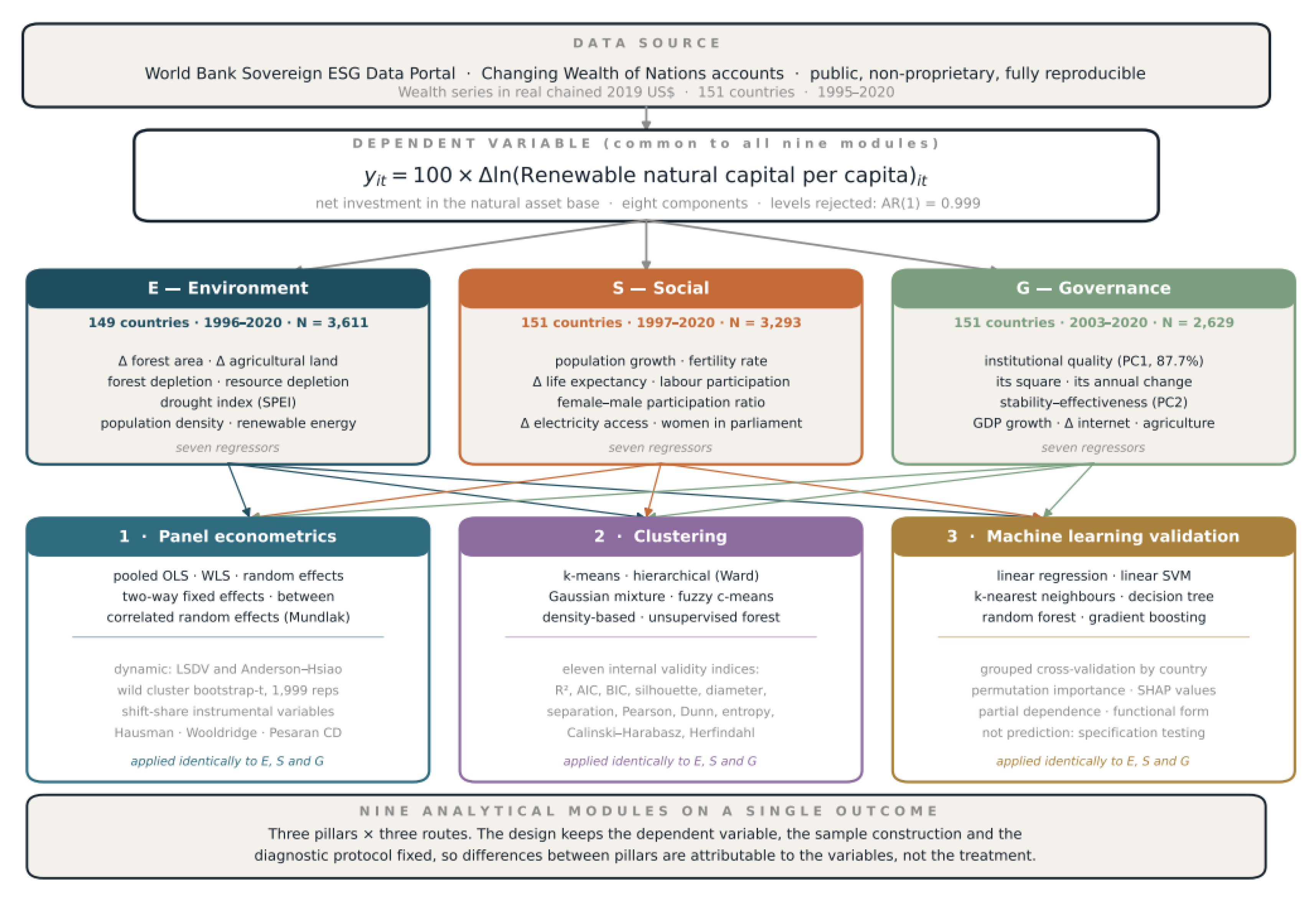
Figure 2.
Renewable natural capital per capita and its share of comprehensive wealth, 1995–2020. Left panel: median across countries with interquartile range. Right panel: median share of national comprehensive wealth.
Figure 2.
Renewable natural capital per capita and its share of comprehensive wealth, 1995–2020. Left panel: median across countries with interquartile range. Right panel: median share of national comprehensive wealth.
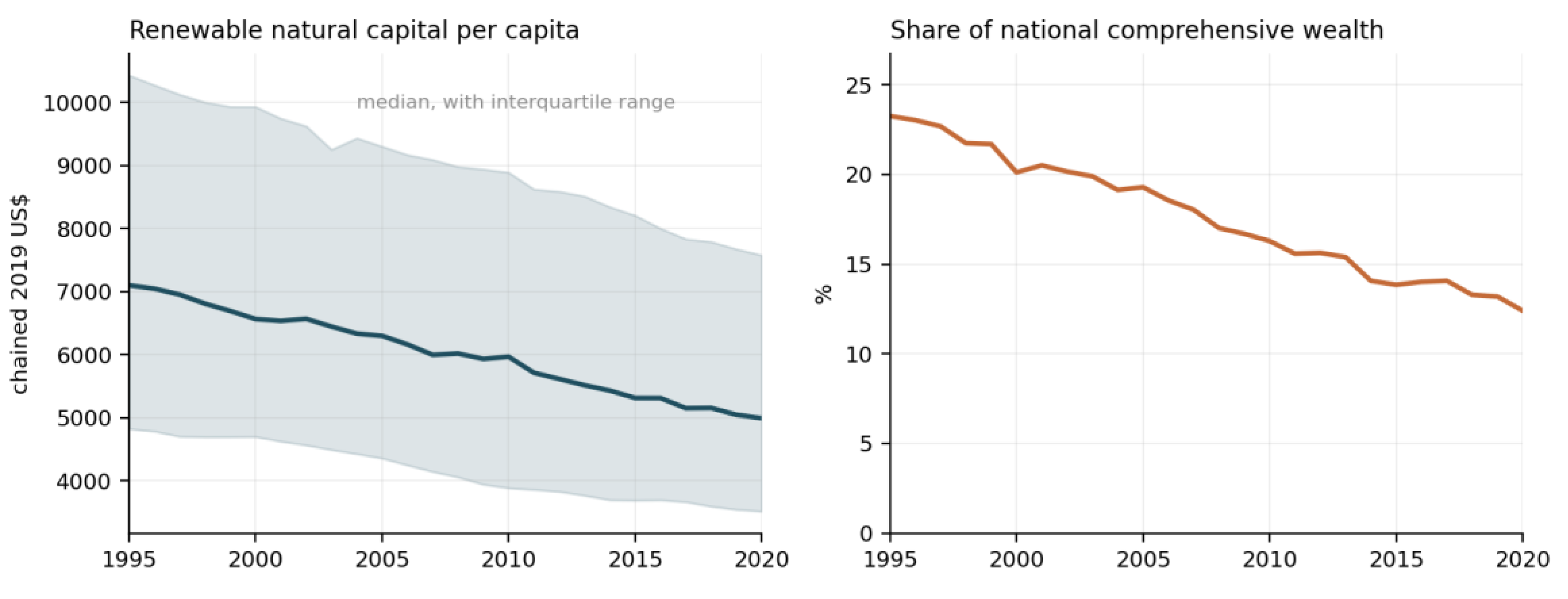
Figure 3.
The renewable energy share and the growth of renewable natural capital per capita in the two panel dimensions. Left panel: country means. Right panel: deviations from country means.
Figure 3.
The renewable energy share and the growth of renewable natural capital per capita in the two panel dimensions. Left panel: country means. Right panel: deviations from country means.
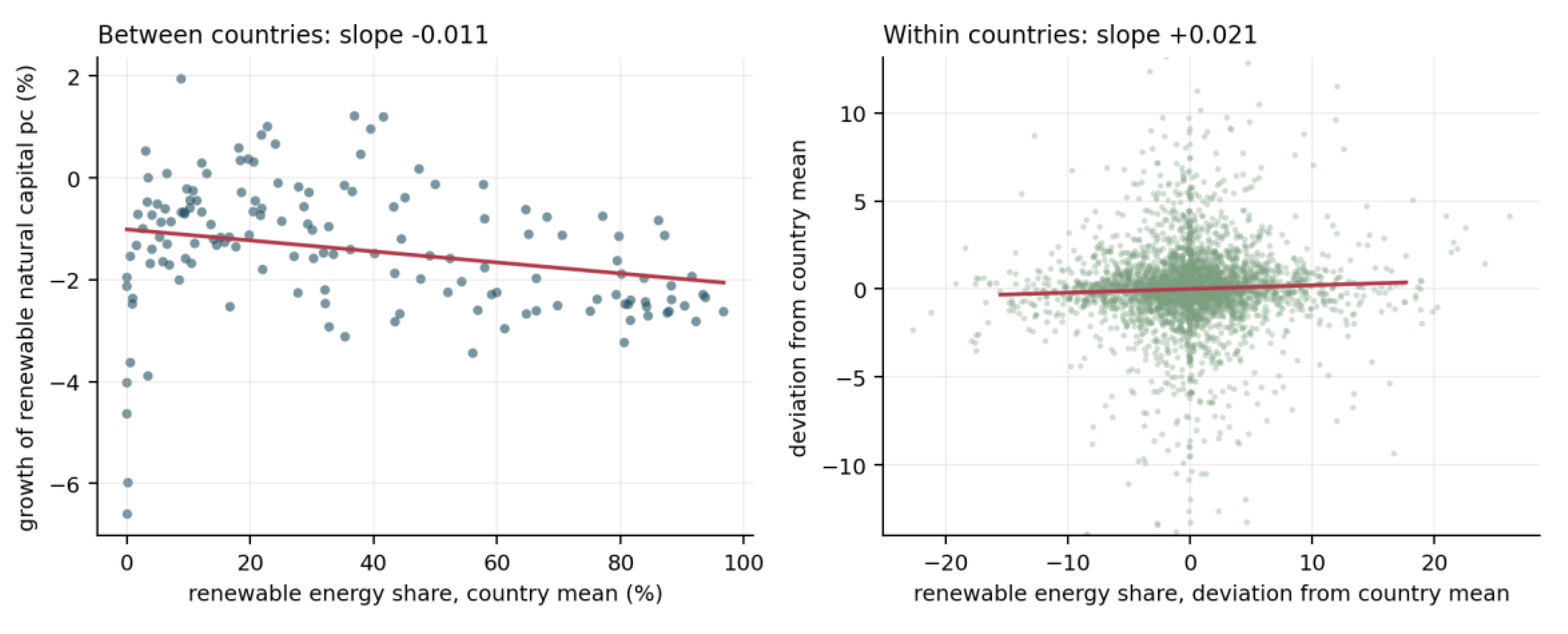
Figure 4.
Cluster profiles. Note. Each bar reports the cluster mean of a variable, expressed in standard deviations from the sample mean.
Figure 4.
Cluster profiles. Note. Each bar reports the cluster mean of a variable, expressed in standard deviations from the sample mean.
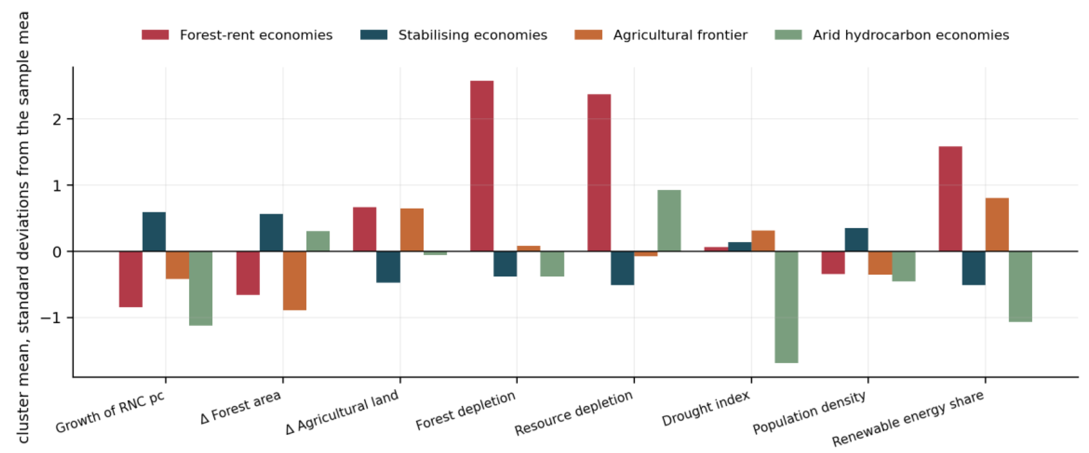
Figure 5.
Random forest attribution against the econometric estimates, environmental block. Left: share of total mean absolute SHAP value by regressor; dark bars mark the coefficients significant in the fixed-effects model after the wild cluster bootstrap. Right: mean absolute SHAP value against the absolute standardised fixed-effects coefficient.
Figure 5.
Random forest attribution against the econometric estimates, environmental block. Left: share of total mean absolute SHAP value by regressor; dark bars mark the coefficients significant in the fixed-effects model after the wild cluster bootstrap. Right: mean absolute SHAP value against the absolute standardised fixed-effects coefficient.
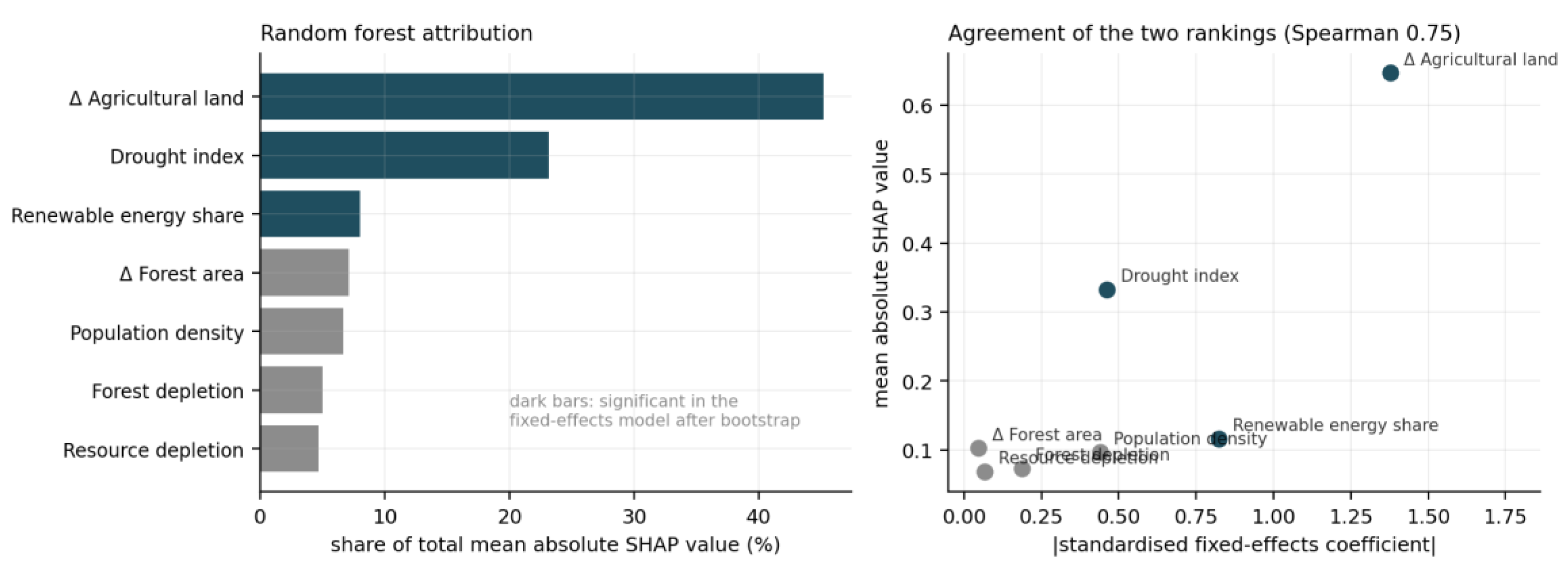
Figure 6.
Left: cross-country mean growth of renewable natural capital, in total and per capita; the shaded area is population growth. Right: country means of total growth against population growth.
Figure 6.
Left: cross-country mean growth of renewable natural capital, in total and per capita; the shaded area is population growth. Right: country means of total growth against population growth.
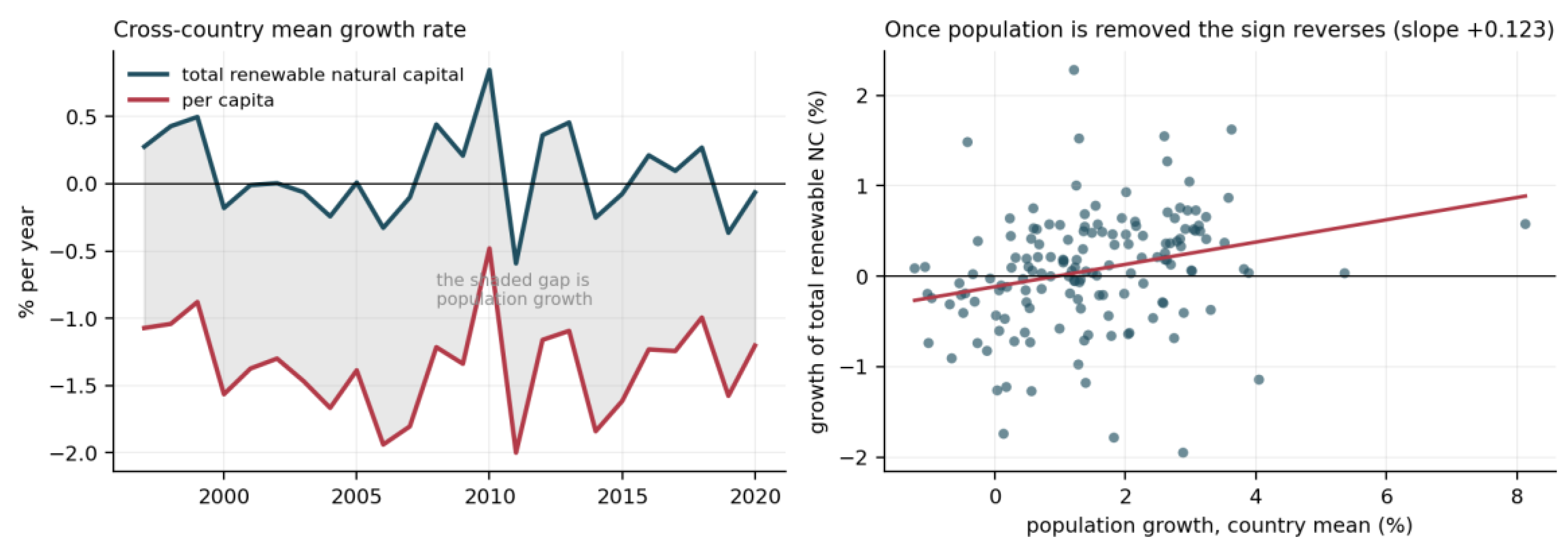
Figure 7.
Cluster profiles for the social block. Note. Each bar reports the cluster mean of a variable, expressed in standard deviations from the sample mean.
Figure 7.
Cluster profiles for the social block. Note. Each bar reports the cluster mean of a variable, expressed in standard deviations from the sample mean.
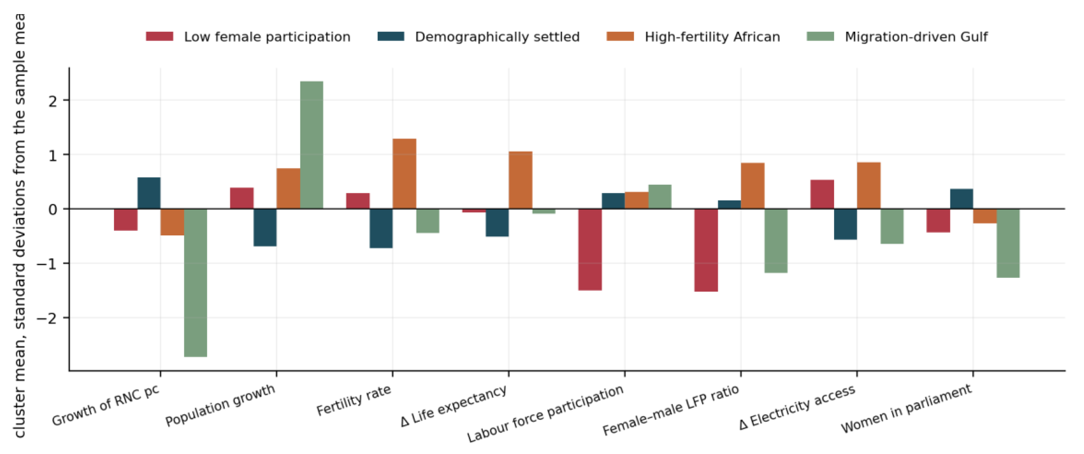
Figure 8.
Share of total mean absolute SHAP value by regressor, with the dependent variable defined per capita on the left and in total on the right. Dark bars mark the coefficients that survived the bootstrap in Section 7; the dashed line marks the share each regressor would receive if all seven contributed equally.
Figure 8.
Share of total mean absolute SHAP value by regressor, with the dependent variable defined per capita on the left and in total on the right. Dark bars mark the coefficients that survived the bootstrap in Section 7; the dashed line marks the share each regressor would receive if all seven contributed equally.
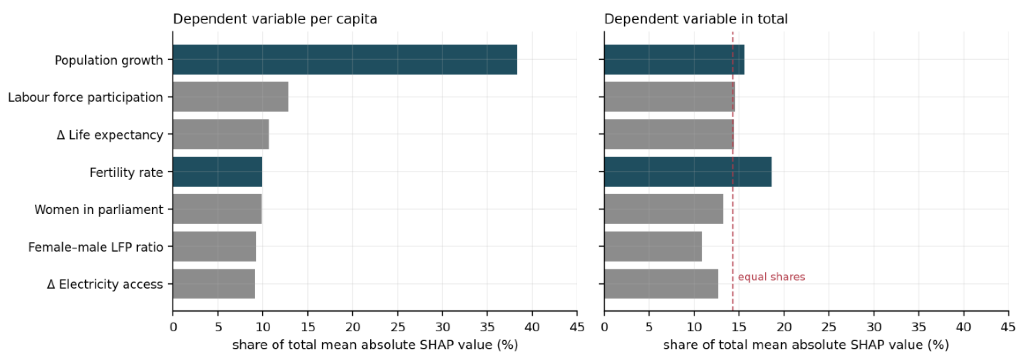
Figure 9.
Left: correlations among the six Worldwide Governance Indicators. Right: variance explained by the principal components of the same six indicators.
Figure 9.
Left: correlations among the six Worldwide Governance Indicators. Right: variance explained by the principal components of the same six indicators.
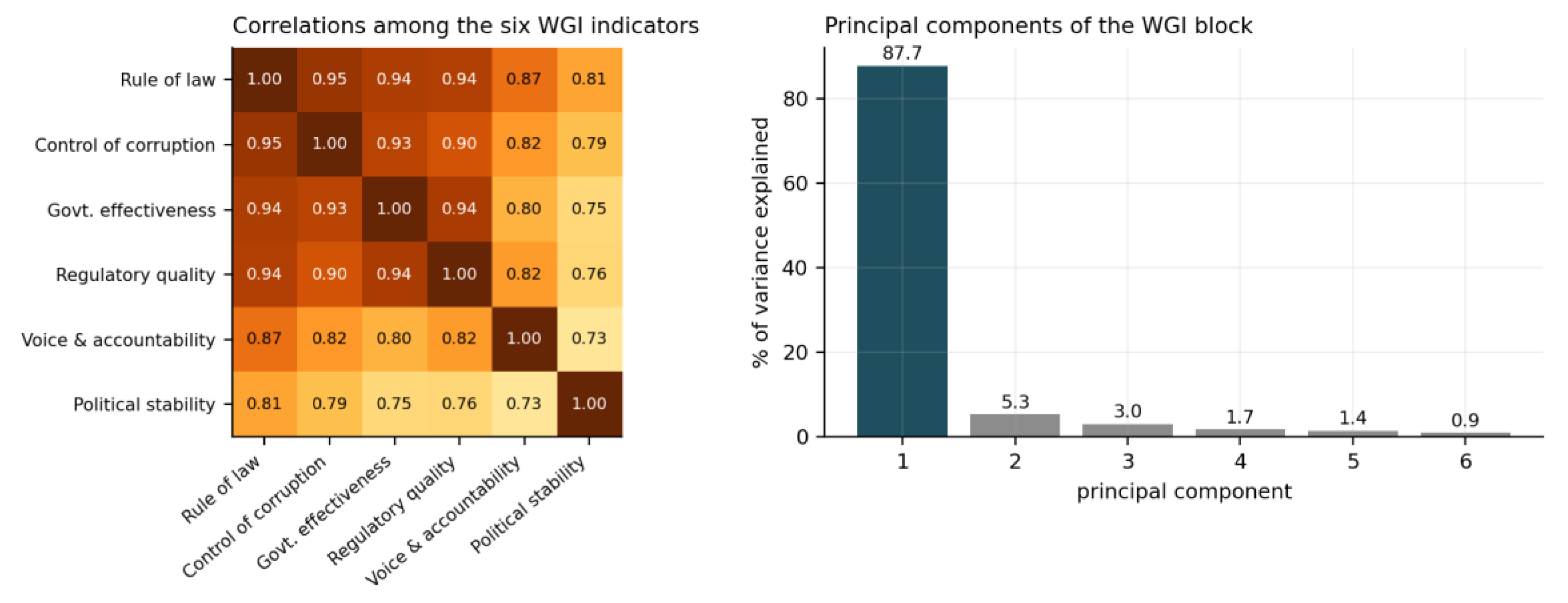
Figure 10.
The annual change in institutional quality and the growth of renewable natural capital per capita. Left: country means, with the horizontal axis expressing the cumulative change over the period. Right: deviations from country means.
Figure 10.
The annual change in institutional quality and the growth of renewable natural capital per capita. Left: country means, with the horizontal axis expressing the cumulative change over the period. Right: deviations from country means.
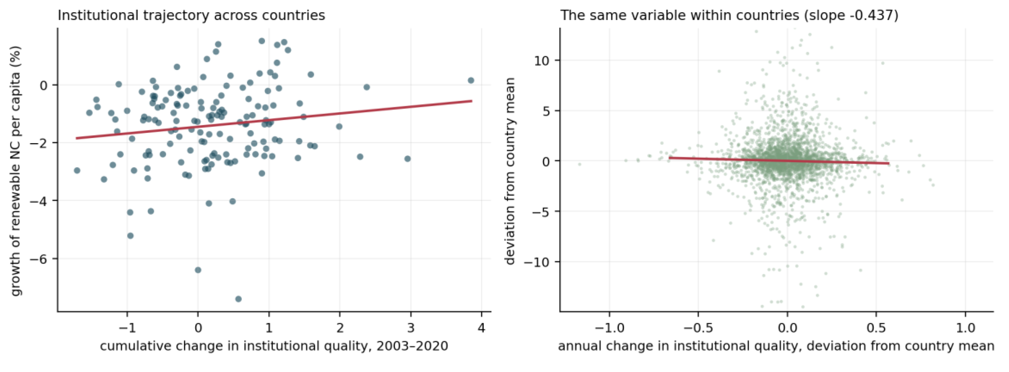
Figure 11.
Cluster profiles for the governance block. Each bar reports the cluster mean of a variable, expressed in standard deviations from the sample mean.
Figure 11.
Cluster profiles for the governance block. Each bar reports the cluster mean of a variable, expressed in standard deviations from the sample mean.
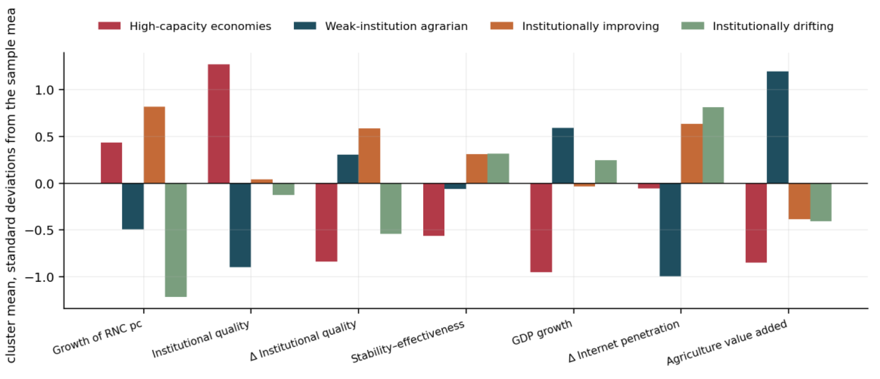
Figure 12.
Left: cross-validated performance of the six learners in the two panel dimensions. Right: in-sample against cross-validated performance in the between dimension, with the diagonal marking equality.
Figure 12.
Left: cross-validated performance of the six learners in the two panel dimensions. Right: in-sample against cross-validated performance in the between dimension, with the diagonal marking equality.
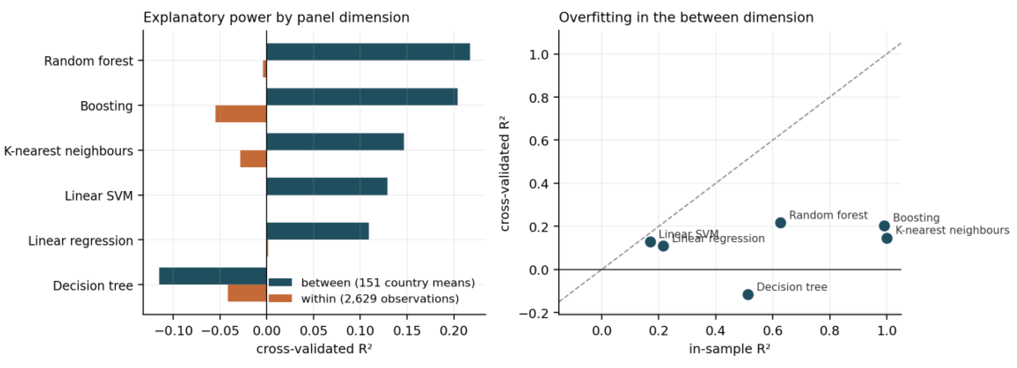
Figure 13.
Share of total mean absolute SHAP value by regressor, computed on country means on the left and on within-transformed observations on the right. Bars in the left panel are dark where the direction of the SHAP contribution matches the sign of the between coefficient.
Figure 13.
Share of total mean absolute SHAP value by regressor, computed on country means on the left and on within-transformed observations on the right. Bars in the left panel are dark where the direction of the SHAP contribution matches the sign of the between coefficient.
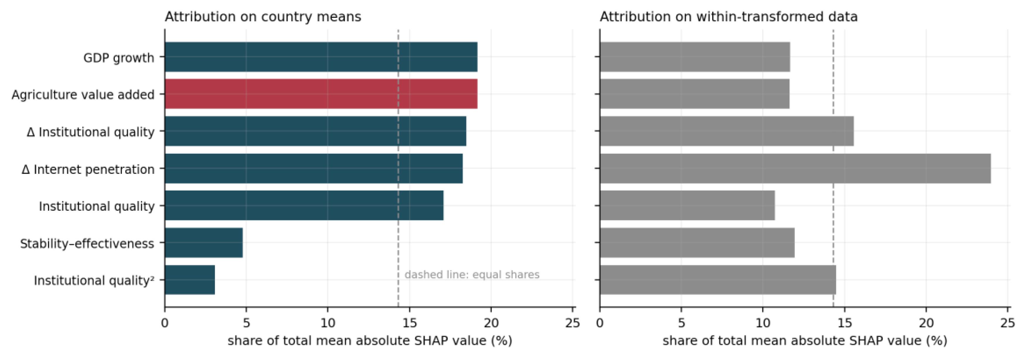
Table 1.
Thematic map of the literature, the gap identified in each strand and the corresponding contribution of this study.
Table 1.
Thematic map of the literature, the gap identified in each strand and the corresponding contribution of this study.
| Research theme | Representative studies | Main gap identified | Contribution of this study |
| Wealth accounting and natural capital measurement (n = 57) | Agarwal & Sawhney, 2021; Ahmad et al., 2018; Aly & Managi, 2018; Balasubramanian, 2018; Bartels et al., 2023; Biasi et al., 2019; Boos, 2015; Chen & Managi, 2026; Chen et al., 2023; Cheng et al., 2022; Cheng et al., 2025; Coulibaly & Managi, 2025; Dasgupta, 2009; Dasgupta, 2010; Dovern et al., 2014; Endo & Ikeda, 2022; Engelbrecht, 2016; Fan et al., 2022; Ferreira et al., 2008; Gani, 2023; Halkos et al., 2018; Hanley et al., 2015; Ikeda & Managi, 2019; Ikeda et al., 2017; Jingyu et al., 2020; Jones, 2024; Jumbri & Managi, 2020; Kim et al., 2023; Kousar et al., 2025; Kumar & Mizunoya, 2022; Li, 2024; Maher et al., 2020; Ollivier & Giraud, 2011; Pearson et al., 2013; Polasky et al., 2015; Resce, 2021; Roman & Thiry, 2016; Sato et al., 2018; Shi et al., 2026; Sugiawan & Managi, 2026; Sugiawan et al., 2019; Sugiawan et al., 2023; Xi et al., 2026; Xie et al., 2026; Xue et al., 2022; Yamaguchi & Managi, 2019; Yamaguchi et al., 2019; Yamaguchi et al., 2023; Yamaguchi, 2014; Yamaguchi, 2020; Yamaguchi, 2021; Yang et al., 2023; Yoshida et al., 2018; Zhang & Sun, 2018; Zhang et al., 2020; Zhang et al., 2021 | The literature measures the stock and reports its decline, but treats the change in the stock as an accounting outcome of a savings identity. Its determinants are not estimated. | Takes the annual change in renewable natural capital per capita as the dependent variable and estimates its determinants for 151 countries over 1995–2020, across three pillar equations and six estimators. |
| Ecosystem service valuation (n = 11) | Ahmed & Jahan, 2026; Ghauri et al., 2022; Mehaffy, 2026; Ovchynnykova et al., 2024; Pacheco et al., 2018; Sharma & Paramati, 2022; Souliotis & Voulvoulis, 2025; Taghikhah et al., 2022; Taljaard et al., 2021; Wolde-Rufael & Mulat-Weldemeskel, 2023; Zank et al., 2016 | Valuation studies are ecological rather than economic in design, are usually confined to one country or biome, and do not connect the valued asset to national accounting aggregates. | Decomposes the dependent variable into its eight accounting components and shows that agricultural land carries 62.1 per cent of the aggregate, quantifying how much of each estimated effect is valuation rather than economics. |
| Land use, climate and the energy mix (n = 8) | Ahmad et al., 2026; Ichsan et al., 2026; Kramarz & Kmiecik, 2026; Mushtaq et al., 2026; Qi et al., 2026; Quiroga-Canaviri et al., 2026; Yang et al., 2021 | Land use and climate variables are studied as outcomes of environmental pressure, not as determinants of the value of the natural asset base; climatic exogeneity is rarely exploited. | Identifies the drought index as the only regressor with a credible claim to exogeneity; its coefficient is positive and significant in all six estimators and rises from 0.457 to 1.113 when agricultural land is removed from the dependent variable. |
| Institutions and the resource curse (n = 34) | Abd El Nasser et al., 2025; Abou Houran & Mehmood, 2023; Adikpo & Usman, 2023; Alsaleh & Abdul-Rahim, 2023; Ameer & Ahmad, 2024; Apaza, 2009; Barut et al., 2026; Bekoe & Jalloh, 2023; Bitassa et al., 2025; Doan et al., 2025; Gong et al., 2023; Herrero Gómez et al., 2026; Huang et al., 2024; Huque & Jongruck, 2018; Idris et al., 2025; Jahanger et al., 2023; Kashif et al., 2024; Kaufmann et al., 2010; Langbein & Knack, 2010; Li et al., 2023; Liu & Waqas, 2024; Munir et al., 2026; Muno, 2012; Naimoğlu & Shahbaz, 2025; Puente De La Vega Caceres et al., 2024; Sawadogo & Ouoba, 2024; Sun et al., 2023; Teklie & Yağmur, 2024; Thomas, 2010; Wang et al., 2022; Wang et al., 2024; Zhang et al., 2023; Zhang et al., 2025; Çiçekçi & Gaygısız, 2023 | Institutions are related to resource rents, extraction and emissions, but not to the accumulation of the natural asset base, and the level of institutional quality is not distinguished from its trajectory. | Separates level from trajectory: the between coefficient on the annual change in institutional quality is 9.096 (p < 0.001) while the within counterpart is −0.198 and insignificant, and the clustering recovers the same distinction without using any coefficient. |
| Demography and the social pillar (n = 10) | Coldwell et al., 2022; García-Rudolph et al., 2021; Kumar, 2025; Lee et al., 2026; Liu et al., 2023; Mushi, 2026; Preusse et al., 2024; Roupakias & Chletsos, 2020; Shi et al., 2023; Yuan et al., 2026 | Population enters as a control or a scaling factor. The accounting role of population growth in per capita wealth measures is not separated from any behavioural effect. | Shows the coefficient on population growth is −0.913, indistinguishable from the −1 implied by the identity, and that it falls to +0.087 (p = 0.306) once the dependent variable is defined on the total rather than the per capita stock. |
| Country-level ESG and composite indices (n = 37) | AL-Barakani et al., 2022; Al-Tahat et al., 2025; Amare et al., 2024; Bonga-Bonga & Kirsten, 2026; Cabral Roque et al., 2026; Cheng et al., 2026; Ciacci et al., 2020; Cook & Davíðsdóttir, 2021; Dong et al., 2024; Du et al., 2022; Hoekstra, 2020; Hwang et al., 2024; Ibrahim & Ajide, 2022; Joshi et al., 2026; Karşiyakali & Çetin, 2025; Khan & Shahid, 2026; Kwilinski et al., 2026; Kılıçaslan et al., 2025; Li & Hassan, 2026; Lior et al., 2018; Liu et al., 2025; Managi et al., 2024; Mondjeli et al., 2024; Nagai, 2026; Nguyen et al., 2023; Ozcan et al., 2026; Qiao et al., 2025; Saba et al., 2024; Saba et al., 2025; Santos et al., 2024; Tiba, 2023; Tweneboah-Koduah et al., 2023; Wang & Baig, 2026; Wang et al., 2023; Wen et al., 2024; Yufenyuy et al., 2025; Zhang & Punjwani, 2025 | Country-level ESG work aggregates the three pillars into composite scores with fixed weights, and applies them to flow measures of environmental pressure rather than to environmental wealth. | Estimates the three pillars as separate and directly comparable equations on one dependent variable, and documents a sign reversal on the renewable energy share that a fixed-weight composite would average away. |
| Panel econometric methods (n = 22) | Apfel, 2024; Borusyak et al., 2022; Borusyak et al., 2025; Breuer, 2022; Broxterman & Larson, 2020; Fauceglia & Slembeck, 2021; Fitchett & Wesselbaum, 2022; Galeana-Pizaña et al., 2026; Goldsmith-Pinkham et al., 2020; Gunji & Miura, 2025; Lowenstein, 2024; Lv et al., 2021; Olaniyi & Odhiambo, 2025; Qu et al., 2026; Song et al., 2026; Tackie et al., 2023; Tambo et al., 2020; van Krevel, 2021; Wang et al., 2025; Wu, 2023; Yin & Edward, 2025; Zheng & Zhang, 2025 | Panel work reports a single preferred estimator and treats the remainder as robustness, leaving the between and within dimensions of each regressor unseparated. | Reports six estimators as a requirement of identification rather than of robustness, with a Mundlak test in each block, wild cluster bootstrap inference over 1,999 replications and shift-share instruments for the regressors where simultaneity is plausible. |
| Machine learning and validation (n = 21) | Achahboun et al., 2026; Alnaqbi et al., 2026; Baffour Gyau et al., 2026; Baigarayeva et al., 2026; Chang et al., 2024; Chen et al., 2025; Clarke & Polselli, 2026; Deist et al., 2018; Drago et al., 2026; Espoir et al., 2026; Hijazi & Moshref, 2026; Iqbal et al., 2025; Kong & Gao, 2024; Liang et al., 2024; Mulenga et al., 2026; Saba & Ngepah, 2022; Sengani et al., 2026; Sodnomdavaa, 2026; Viswanathan et al., 2026; Zhang & Yin, 2026; Zhao et al., 2023 | Machine learning is used for prediction and for feature ranking, seldom as an instrument for validating the functional form and the attribution of an econometric specification. | Uses six supervised learners not to predict but to validate: the linear specification wins out of sample in every block, and SHAP attribution independently recovers the three regressors that survive the bootstrap in the environmental equation. |
Note. Two hundred studies are assigned to exactly one theme, so the counts sum to two hundred.
Table 2.
Environmental determinants of the growth of renewable natural capital per capita, 1996–2020. Country-clustered standard errors in parentheses, robust errors for the between estimator.
Table 2.
Environmental determinants of the growth of renewable natural capital per capita, 1996–2020. Country-clustered standard errors in parentheses, robust errors for the between estimator.
| Variable | Pooled OLS | WLS | RE | FE (two-way) | Between | CRE |
| Δ Forest area | 1.0232** (0.4025) | 0.8759** (0.4459) | 0.4205 (0.3498) | −0.1706 (0.2725) | 1.9909*** (0.4740) | −0.1985 (0.2643) |
| Δ Agricultural land | 1.2435*** (0.1136) | 0.7584*** (0.1071) | 1.2921*** (0.1147) | 1.3377*** (0.1188) | 0.5602* (0.3030) | 1.3371*** (0.1164) |
| Net forest depletion | 0.0396* (0.0229) | 0.0323** (0.0137) | 0.0336* (0.0201) | 0.0429 (0.0276) | 0.0427 (0.0278) | 0.0473* (0.0267) |
| Natural resources depletion | −0.0731*** (0.0198) | −0.0082 (0.0130) | −0.0584*** (0.0161) | −0.0095 (0.0133) | −0.0721*** (0.0211) | −0.0186 (0.0135) |
| Drought index (SPEI) | 0.5296*** (0.1067) | 0.1393*** (0.0303) | 0.4789*** (0.1100) | 0.4571*** (0.1147) | 1.0556*** (0.2900) | 0.4524*** (0.1135) |
| Population density (log) | −0.1015 (0.0737) | 0.2098*** (0.0579) | −0.0697 (0.0717) | 0.3195 (0.4975) | −0.0890 (0.0767) | 0.7827** (0.3832) |
| Renewable energy share | −0.0133*** (0.0035) | −0.0203*** (0.0047) | −0.0133*** (0.0032) | 0.0274*** (0.0085) | −0.0103*** (0.0038) | 0.0287*** (0.0084) |
| Constant | −0.0850 (0.3568) | −1.5688*** (0.2973) | −0.3197 (0.3451) | −3.6913* (2.2306) | −0.0863 (0.3868) | −0.0621 (0.3756) |
| R2 | 0.191 | 0.371 | 0.186 | 0.191 | 0.343 | 0.199 |
| Observations | 3,611 | 3,611 | 3,611 | 3,611 | 149 | 3,611 |
Note. Significance: *** p<0.01; ** p<0.05; * p<0.10.
Table 3.
Comparison of six clustering algorithms, 149 countries, k = 4.
| Algorithm | R2 | AIC | BIC | Silhouette | Calinski–Harabasz | Mean rank |
| K-Means | 0.444 | −628.0 | −519.9 | 0.253 | 38.62 | 2.50 |
| Hierarchical | 0.416 | −568.8 | −460.7 | 0.219 | 34.41 | 2.77 |
| Fuzzy c-means | 0.362 | −463.3 | −355.2 | 0.139 | 27.40 | 3.50 |
| Model-based | 0.391 | −520.0 | −411.9 | 0.198 | 31.09 | 3.55 |
| Density-based | 0.192 | −182.3 | −74.2 | 0.223 | 11.49 | 4.27 |
| Random forest | 0.322 | −391.5 | −283.4 | 0.034 | 22.97 | 4.41 |
Note. Panel A: indices of fit and compactness. Higher values are preferred for explained variance, the silhouette and the Calinski–Harabasz statistic, lower values for the information criteria. The mean rank in the final column is computed over all eleven indices, including those in Panel B.
Table 4.
Comparison of six clustering algorithms, 149 countries, k = 4.
| Algorithm | Max diameter | Min separation | Pearson | Dunn | Entropy | HHI |
| K-Means | 7.704 | 0.717 | −0.550 | 0.093 | 1.137 | 0.375 |
| Hierarchical | 7.704 | 1.289 | −0.499 | 0.167 | 1.104 | 0.401 |
| Fuzzy c-means | 8.210 | 0.859 | −0.392 | 0.105 | 1.309 | 0.289 |
| Model-based | 7.649 | 0.686 | −0.442 | 0.090 | 1.140 | 0.359 |
| Density-based | 8.615 | 1.753 | −0.631 | 0.203 | 0.621 | 0.688 |
| Random forest | 8.210 | 0.771 | −0.340 | 0.094 | 1.180 | 0.343 |
Table 6.
Social determinants of the growth of renewable natural capital per capita, 1997–2020.
| Variable | Pooled OLS | WLS | RE | FE (two-way) | Between | CRE |
| Population growth | −0.9638*** (0.0496) | −0.8180*** (0.1053) | −0.9638*** (0.0496) | −0.9132*** (0.0847) | −0.9945*** (0.0544) | −0.9087***(0.0807) |
| Fertility rate | 0.1545*** (0.0447) | 0.0241 (0.0915) | 0.1545*** (0.0447) | 0.5368*** (0.2027) | 0.1373** (0.0583) | 0.4370*** (0.1571) |
| Δ Life expectancy | −0.0170 (0.0312) | 0.0007 (0.0060) | −0.0170 (0.0312) | −0.0283 (0.0284) | 0.2130 (0.3123) | −0.0273 (0.0338) |
| Labour force participation | 0.0157*** (0.0054) | 0.0205** (0.0098) | 0.0157*** (0.0054) | 0.0072 (0.0290) | 0.0165*** (0.0055) | 0.0088 (0.0270) |
| Female–male LFP ratio | −0.0007 (0.0031) | −0.0074 (0.0061) | −0.0007 (0.0031) | 0.0106 (0.0188) | −0.0024 (0.0036) | 0.0160 (0.0178) |
| Δ Electricity access | −0.0060 (0.0157) | −0.0098 (0.0084) | −0.0060 (0.0157) | −0.0092 (0.0161) | 0.0358 (0.0616) | −0.0061(0.0148) |
| Women in parliament | −0.0008 (0.0040) | 0.0069 (0.0067) | −0.0008 (0.0040) | −0.0187* (0.0107) | 0.0022 (0.0049) | −0.0074 (0.0095) |
| R2 | 0.158 | 0.527 | 0.158 | 0.055 | 0.820 | 0.160 |
| Observations | 3,293 | 3,293 | 3,293 | 3,293 | 151 | 3,293 |
Note. Country-clustered standard errors in parentheses, robust errors for the between estimator. Significance: *** p<0.01; ** p<0.05; * p<0.10.
Table 7.
Comparison of six clustering algorithms on the social block, 151 countries, k = 4. Panel A: indices of fit and compactness.
Table 7.
Comparison of six clustering algorithms on the social block, 151 countries, k = 4. Panel A: indices of fit and compactness.
| Algorithm | R2 | AIC | BIC | Silhouette | Calinski–Harabasz | Mean rank |
| K-Means | 0.515 | −802.2 | −693.6 | 0.344 | 52.04 | 2.18 |
| Hierarchical | 0.477 | −710.5 | −601.8 | 0.311 | 44.65 | 2.45 |
| Fuzzy c-means | 0.488 | −736.0 | −627.3 | 0.170 | 46.65 | 3.36 |
| Random forest | 0.467 | −688.3 | −579.7 | 0.272 | 42.95 | 3.64 |
| Model-based | 0.454 | −660.1 | −551.5 | 0.128 | 40.83 | 4.64 |
| Density-based | 0.388 | −520.7 | −412.1 | 0.266 | 31.04 | 4.73 |
Note. The mean rank in the final column is computed over all eleven indices, including those of Panel B.
Table 8.
Comparison of six clustering algorithms on the social block, 151 countries, k = 4.
| Algorithm | Max diameter | Min separation | Pearson | Dunn | Entropy | HHI |
| K-Means | 7.722 | 0.890 | −0.672 | 0.115 | 1.122 | 0.375 |
| Hierarchical | 8.227 | 1.225 | −0.662 | 0.149 | 1.178 | 0.371 |
| Fuzzy c-means | 9.821 | 0.788 | −0.486 | 0.080 | 1.362 | 0.263 |
| Random forest | 9.270 | 0.956 | −0.647 | 0.103 | 1.130 | 0.372 |
| Model-based | 9.821 | 0.726 | −0.428 | 0.074 | 1.367 | 0.259 |
| Density-based | 9.821 | 1.227 | −0.567 | 0.125 | 1.081 | 0.399 |
Note. Panel B: indices of separation and of the size distribution.
Table 9.
Comparison of six supervised learners on the residualised social equation, dependent variable per capita, 3,293 observations, ten-fold cross-validation grouped by country.
Table 9.
Comparison of six supervised learners on the residualised social equation, dependent variable per capita, 3,293 observations, ten-fold cross-validation grouped by country.
| Model | Cross-validated R2 | RMSE | MAE | In-sample R2 | Overfitting gap |
| Linear SVM | 0.0520 | 3.154 | 1.574 | 0.054 | 0.002 |
| Linear regression | 0.0516 | 3.155 | 1.580 | 0.055 | 0.004 |
| Random forest | 0.0381 | 3.177 | 1.649 | 0.433 | 0.395 |
| Decision tree | 0.0178 | 3.211 | 1.695 | 0.086 | 0.068 |
| K-nearest neighbours | 0.0113 | 3.221 | 1.717 | 1.000 | 0.989 |
| Boosting | −0.0038 | 3.246 | 1.728 | 0.481 | 0.485 |
Table 10.
Governance determinants of the growth of renewable natural capital per capita, 2003–2020. Country-clustered standard errors in parentheses, robust errors for the between estimator.
Table 10.
Governance determinants of the growth of renewable natural capital per capita, 2003–2020. Country-clustered standard errors in parentheses, robust errors for the between estimator.
| Variable | Pooled OLS | WLS | RE | FE (two-way) | Between | CRE |
| Institutional quality | 0.1203** (0.0479) | 0.0519 (0.0786) | 0.1079** (0.0466) | 0.1841 (0.2200) | 0.1666*** (0.0550) | 0.2025 (0.2146) |
| Institutional quality2 | −0.0155 (0.0150) | −0.0454* (0.0237) | −0.0053 (0.0147) | 0.1364*** (0.0527) | −0.0308 (0.0191) | 0.1178** (0.0481) |
| Δ Institutional quality | 0.1970 (0.3459) | 0.3127 (0.1929) | −0.1423 (0.3514) | −0.1984 (0.3952) | 9.0956*** (2.0457) | −0.4336 (0.3758) |
| Stability–effectiveness | −0.1692 (0.1731) | −0.4424* (0.2427) | −0.1450 (0.1620) | 0.0517 (0.2641) | −0.1916 (0.2088) | −0.0192 (0.2699) |
| GDP growth | −0.0475* (0.0247) | 0.0100 (0.0151) | −0.0351* (0.0198) | −0.0166 (0.0201) | −0.2475** (0.1024) | −0.0245 (0.0173) |
| Δ Internet penetration | −0.0281 (0.0222) | 0.0182 (0.0117) | −0.0337* (0.0204) | −0.0434** (0.0207) | 0.0688 (0.1184) | −0.0386* (0.0203) |
| Agriculture value added | −0.0139 (0.0109) | −0.0148 (0.0113) | −0.0132 (0.0103) | 0.0125 (0.0243) | 0.0000 (0.0175) | 0.0038 (0.0225) |
| R2 | 0.016 | 0.155 | 0.008 | 0.005 | 0.216 | 0.020 |
| Observations | 2,629 | 2,629 | 2,629 | 2,629 | 151 | 2,629 |
Note. Significance: *** p<0.01; ** p<0.05; * p<0.10.
Table 11.
Comparison of six clustering algorithms on the governance block, 151 countries, k = 4.
| Algorithm | R2 | AIC | BIC | Silhouette | Calinski–Harabasz | Mean rank |
| K-Means | 0.453 | −573.9 | −477.4 | 0.217 | 40.60 | 1.91 |
| Hierarchical | 0.416 | −504.2 | −407.6 | 0.196 | 34.88 | 2.45 |
| Fuzzy c-means | 0.426 | −523.6 | −427.0 | 0.183 | 36.43 | 2.73 |
| Model-based | 0.365 | −415.8 | −319.3 | 0.115 | 28.15 | 4.18 |
| Random forest | 0.359 | −405.5 | −309.0 | 0.109 | 27.40 | 4.36 |
| Density-based | 0.180 | −146.3 | −49.8 | 0.029 | 10.79 | 5.36 |
Note. Panel A: indices of fit and compactness. The mean rank is computed over all eleven indices, including those of Panel B.
Table 12.
Comparison of six clustering algorithms on the governance block, 151 countries, k = 4.
| Algorithm | Max diameter | Min separation | Pearson | Dunn | Entropy | HHI |
| K-Means | 6.024 | 0.842 | −0.467 | 0.140 | 1.353 | 0.266 |
| Hierarchical | 6.551 | 1.147 | −0.480 | 0.175 | 1.157 | 0.363 |
| Fuzzy c-means | 7.126 | 0.557 | −0.433 | 0.078 | 1.379 | 0.253 |
| Model-based | 7.477 | 0.482 | −0.335 | 0.064 | 1.372 | 0.257 |
| Random forest | 7.211 | 0.957 | −0.471 | 0.133 | 1.062 | 0.409 |
| Density-based | 8.371 | 1.056 | −0.236 | 0.126 | 1.031 | 0.408 |
Note. Panel B: indices of separation and of the size distribution.
Table 13.
Comparison of six supervised learners on the governance equation in the two panel dimensions.
Table 13.
Comparison of six supervised learners on the governance equation in the two panel dimensions.
| Model | Within: CV R2 | Within: gap | Between: CV R2 | Between: RMSE | Between: gap |
| Random forest | −0.0042 | 0.421 | 0.2172 | 1.235 | 0.409 |
| Boosting | −0.0547 | 0.563 | 0.2039 | 1.246 | 0.787 |
| K-nearest neighbours | −0.0286 | 1.029 | 0.1468 | 1.290 | 0.853 |
| Linear SVM | 0.0004 | 0.002 | 0.1291 | 1.303 | 0.041 |
| Linear regression | 0.0013 | 0.004 | 0.1090 | 1.318 | 0.107 |
| Decision tree | −0.0416 | 0.112 | −0.1153 | 1.474 | 0.629 |
Note. The within columns use 2,629 residualised observations with folds grouped by country; the between columns use 151 country means with ten-fold cross-validation. The gap is the difference between in-sample and cross-validated performance.
Table 14.
Synthesis of the nine modules; E denotes the environmental pillar, S the social and G the governance pillar.
Table 14.
Synthesis of the nine modules; E denotes the environmental pillar, S the social and G the governance pillar.
| Pillar | Panel econometrics | Clustering | Machine learning validation |
| E | Three of seven coefficients survive the bootstrap. The drought index is positive and significant in all six estimators (+0.457, p < 0.001) and rises to 1.113 when agricultural land is excluded. The renewable energy share reverses sign between dimensions: −0.010 between, +0.027 within. Within R2 0.191, between R2 0.343. | Four types at k = 4; k-means preferred (mean rank 2.50). Aridity is the sharpest discriminant of any variable in any block, at −1.69 standard deviations, and identifies the group losing natural capital fastest (−2.85% a year). Silhouette 0.253. | The linear model wins out of sample (0.184 against 0.140 for the random forest); interactions and squares do not help. SHAP independently recovers the same three regressors, at 45.2%, 23.2% and 8.1% of attribution. Confirms and refines. |
| S | The coefficient on population growth is −0.913, indistinguishable from the −1 implied by the accounting identity, and falls to +0.087 (p = 0.306) on the total stock. Fertility survives the decomposition (+0.537) and operates through cultivated land. Within R2 0.055, between R2 0.820. | Four types at k = 4, the cleanest partition of the three (silhouette 0.344). The migration-driven Gulf group, six countries with fertility below the sample mean, loses 5.08% a year — recovering the identity as the defining feature of the extreme case. | The linear model wins again (0.052 against 0.038). Attribution concentrates 38.3% on population growth when the identity is present and disperses almost uniformly when it is removed. Confirms but subtracts: on the total stock, CV R2 is 0.001. |
| G | Almost no temporal content: within R2 0.005 and no coefficient survives the bootstrap. The cross-section is informative, with Δ institutional quality at +9.096 and its level at +0.167, both significant, and a Mundlak statistic of 43.37. Between R2 0.216. | Four types, the weakest partition (silhouette 0.217) and the failure of density-based clustering, which leaves 49 countries unassigned. Two groups at the same institutional level but opposite trajectories differ by 2.84 points a year (−0.27 against −3.11). | The only block where flexibility helps, and only across countries: random forest 0.217 against 0.109 for the linear model, stable over ten partitions. Six of seven SHAP directions match the between coefficients. Signals an omission. |
Note. Each cell reports what the method established for that pillar on the common dependent variable, the annual change in renewable natural capital per capita.
Disclaimer/Publisher’s Note: The statements, opinions and data contained in all publications are solely those of the individual author(s) and contributor(s) and not of MDPI and/or the editor(s). MDPI and/or the editor(s) disclaim responsibility for any injury to people or property resulting from any ideas, methods, instructions or products referred to in the content. |
© 2026 by the authors. Licensee MDPI, Basel, Switzerland. This article is an open access article distributed under the terms and conditions of the Creative Commons Attribution (CC BY) license (http://creativecommons.org/licenses/by/4.0/).
Copyright: This open access article is published under a Creative Commons CC BY 4.0 license, which permit the free download, distribution, and reuse, provided that the author and preprint are cited in any reuse.